Missing Giants: Predictions on Dust-Obscured Galaxy Stellar Mass Assembly Throughout Cosmic Time
Abstract
Due to their extremely dust-obscured nature, much uncertainty still exists surrounding the stellar mass growth and content in dusty, star-forming galaxies (DSFGs) at . In this work, we present a numerical model built using empirical data on DSFGs to estimate their stellar mass contributions across the first 10 Gyr of cosmic time. We generate a dust-obscured stellar mass function that extends beyond the mass limit of star-forming stellar mass functions in the literature, and predict that massive DSFGs constitute as much as of all star-forming galaxies with M M⊙ at . We predict the number density of massive DSFGs and find general agreement with observations, although more data is needed to narrow wide observational uncertainties. We forward model mock massive DSFGs to their quiescent descendants and find remarkable agreement with observations from the literature demonstrating that, to first order, massive DSFGs are a sufficient ancestral population to describe the prevalence of massive quiescent galaxies at . We predict that massive DSFGs and their descendants contribute as much as to the cosmic stellar mass density during the peak of cosmic star formation, and predict an intense epoch of population growth during the Gyr from to 3 during which the majority of the most massive galaxies at high- grow and then quench. Future studies seeking to understand massive galaxy growth and evolution in the early Universe should strategize synergies with data from the latest observatories (e.g. JWST and ALMA) to better include the heavily dust-obscured galaxy population.
1 Introduction
Most of what we understand about galaxy evolution in the first six billion years of the Universe is largely based on rest-frame ultraviolet-to-optical studies. This includes, but is not limited to: the evolution of the galaxy stellar mass function (e.g. Peng et al., 2010; Muzzin et al., 2013; Davidzon et al., 2017; Thorne et al., 2021) used to describe the growth of galaxies over time; the large scale structure of galaxies (e.g. Eisenstein et al., 2011; Zehavi et al., 2011) that demonstrates how galaxies are distributed throughout space as they form and grow; and the star-forming main sequence (e.g. Whitaker et al. 2014 and Table 3 in Speagle et al. 2014) establishing that the majority of galaxies form their stars steadily, over long periods of time ( Gyr), at a rate proportional to their stellar mass. These hereinafter referred to as ‘UV/OP-based’ relationships are often perceived as fundamental truths that are either fed into or used as benchmarks for success in testing our best cosmological models (e.g. Somerville & Davé, 2015; Wechsler & Tinker, 2018). In other words, our primary understanding of galaxy evolution – from observations to simulations – is deeply and intricately rooted in UV/optical astronomy, including all of its strengths and limitations.
It is now well known that the rest-frame UV/optical spectrum of the Universe contains only a piece of the larger picture on star formation in the cosmos. Nearly half of all cosmic starlight in the Universe is obscured by dust (Driver et al., 2008), which re-radiates at longer infrared wavelengths. This phenomenon is most evident in the cosmic star formation rate density where, out to , the majority of stellar mass is built in regions obscured by dust and thus primarily detected via infrared (IR) observations (see Madau & Dickinson, 2014, for a review). This means that studies using only UV/optical to chart stellar mass assembly throughout cosmic time are incomplete and biased against significantly dusty systems.
Over the last two decades, wide-field far-IR and submillimeter surveys ( m) have discovered significant populations of dusty, star-forming galaxies (DSFGs, see Casey, Narayanan, & Cooray 2014 for a review). Though rare in the local Universe, DSFGs are a thousand times more populous at (e.g. Simpson et al., 2014; Zavala et al., 2021), dominating cosmic star formation during these times. Their extreme rates of star formation ( M⊙ yr-1) generate massive reservoirs of dust that obscures the starlight, making some DSFGs nearly invisible to even the deepest UV/optical/near-IR observations, but bright like beacons at far-IR and (sub)millimeter wavelengths (e.g. da Cunha et al., 2015; Williams et al., 2019; Manning et al., 2022).
While some DSFGs are detected in the deepest of UV/optical/near-IR surveys, they are generally left out of large surveys broadly describing galaxy evolution. This usually happens through e.g. stringent requirements for photometric coverage over the rest-frame UV/optical spectrum (e.g. requiring r, i, and z-band detections, Sherman et al., 2020), and/or “redder” selection bands with observations that are still insufficiently deep to capture the heavily obscured (and redshifted) starlight (e.g. Ks-band 24 mag, Lee et al., 2015). While often the best available tool for such studies, these requirements are biased against sources with significant attenuation in their UV/optical spectral energy distributions (SEDs); and, if DSFGs are captured, they are often treated as contaminants to the broader goals of the study, to be either removed or ignored as an insignificantly small portion of the broader galaxy population (e.g. at its peak fraction Sargent et al., 2012; Hwang et al., 2021). Thus, it is likely that several of the fundamental UV/OP-based scaling relations used to describe galaxy evolution and inform our finest models and simulations are lacking a proper accounting of the DSFG population – a population that drives and dominates stellar mass assembly in the first billion years of the cosmos.
Indeed, the astrophysical community has been struggling to properly model and reproduce DSFG populations – and their measured physical characteristics – since their discovery (e.g. Granato et al., 2000; Baugh et al., 2005; Hopkins et al., 2010; Hayward et al., 2013; Aoyama et al., 2019; McAlpine et al., 2019). This may have to do with a need for more sophisticated dust radiative transfer treatments, degeneracies in constraining DSFG stellar initial mass functions, complex dust and star geometries, and/or a general lack of constraints on the physical origins / triggering mechanisms of DSFGs (see e.g. Hayward et al. 2021 for an in depth discussion). Many of the same simulations struggling to properly reproduce DSFG population observations also struggle to produce sufficient populations of massive (M M⊙) quiescent galaxies at early times (e.g. Brennan et al., 2015; Merlin et al., 2019). It is possible that these mysteries and shortcomings are related because it is also likely that these galaxy sub-populations are related.
Several lines of evidence suggest that the brightest DSFGs constitute the primary ancestral population of the most massive quiescent galaxies in the Universe. This includes comparable comoving number densities (n Mpc-3, e.g. Toft et al., 2014; Simpson et al., 2014), dark matter halo masses and clustering properties (M M⊙, e.g. Hickox et al., 2012; Lim et al., 2020), physical shapes and effective radii (r kpc, e.g. Hodge et al., 2016), star formation histories (strong and bursty with SFRs M⊙ yr-1over 50-100 Myr, e.g. Valentino et al., 2020), and stellar masses ( M⊙, e.g. da Cunha et al., 2015; Miettinen et al., 2017). Prior studies have also demonstrated a clear relationship between stellar mass and dustiness, where the most massive galaxies are more dust-obscured across cosmic time (van Dokkum et al., 2006; Pannella et al., 2009; Wuyts et al., 2011; Whitaker et al., 2012, 2017; Deshmukh et al., 2018). Recent discoveries of massive, quiescent galaxies demand short, bursty star-formation histories in line with those exhibited by DSFGs (e.g. Glazebrook et al., 2017; Schreiber et al., 2018a). And, finally, the shark semi-analytical model (which is largely successful in modeling on-sky DSFG populations) suggests that the majority of the most massive galaxies (M M⊙) at undergo a (sub)millimeter-bright phase at (e.g. Lagos et al., 2020). Thus, in order for us to understand how the most massive galaxies form and quench during the first half of the cosmic time, it is of the utmost importance that we are dogged in our pursuit towards understanding massive, dust-obscured galaxies and placing them into the wider context of massive galaxy evolution at .
The objectives of this work are twofold. The first is to quantify, to first-order, the significance of missing DSFG populations at the massive end of the star-forming galaxy stellar mass function (SMF). Star-forming SMFs are biased against dusty galaxies as they are determined using UV/optical tracers. Infrared luminosity functions, however, primarily trace dust emission from the star-forming regions of galaxies. Combined, the UV/OP and IR luminosity functions make up the cosmic star formation rate density known today (Madau & Dickinson, 2014). Still missing from the picture, however, is a evolutionary depiction of the stellar mass contributions from dust-obscured star-forming galaxies. Using the IR luminosity function as a nearly-complete consensus of DSFGs out to , we seek to quantify what the dust-obscured stellar mass function might look like, and posit that it would generate more numerous massive galaxies than previously measured in UV/OP-based SMFs.
The second objective is to test the hypothesis that, despite the heterogeneity of the DSFG population, it is sufficient and complete enough to describe and model the assembly of massive quiescent galaxies in the early Universe. Using a suite of simple assumptions to forward evolve mock populations of DSFGs, we are able to reproduce the observed evolution of massive, passive galaxies – without needing to invoke any complex assumptions on merger histories, feedback / quenching mechanisms, or even contributions from outside populations (e.g. blue nuggets, Miettinen et al., 2017).
This paper is organized as follows: in Section 2 we describe the basis assumptions and empirical data used to build the model used in our analysis; in Section 3.1 we describe the resulting dust-obscured stellar mass function from our model and how we forward evolve mock galaxies to create their quiescent descendants (Sec. 4.3.1); in Section 4 we present the number and stellar mass density predictions and compare to those in the literature; in Section 5, we discuss some additional implications of this model, and provide a summary in Section 6. Throughout this work, we adopt a Planck cosmology, where km s-1 Mpc-1 and (Planck Collaboration et al., 2016); where relevant, we adopt a Chabrier IMF (Chabrier, 2003).
2 Model Ingredients
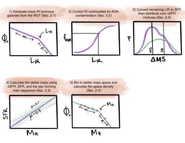
Recent theoretical and observational show that the most massive star-forming galaxies in the Universe are heavily obscured by dust. This would mean that a significant portion of cosmic stellar mass is enshrouded in dust, and therefore difficult to detect with traditional photometric methods in the rest-frame UV/optical spectrum. Our goal in this work is to use existing empirical data on dusty, star-forming galaxies to test this hypothesis and quantify the impact of DSFGs on the massive end of galaxy evolution. In this section, we describe the empirical data and assumptions used to build our numerical model, as well as the model itself. There are four main steps to populate the model, each described and motivated in greater detail in the proceeding subsections. We:
-
1.
Use the infrared luminosity function to derive a mock population of DSFGs (Section 2.1).
-
2.
Correct IR luminosities for AGN contamination so that LIR accounts for only star formation emission (Section 2.2).
-
3.
Convert LIR to SFR and distribute SFRs over the star-forming main sequence (i.e. the M∗-SFR relation) to derive stellar masses for the mock DSFGs (Section 2.3).
-
4.
Bin in stellar mass space and compute the volume-averaged stellar mass density (Section 2.4).
In Figure 1, we share a cartoon depiction of our model. The model is realized in a light cone of solid angle 1 deg2 over a given redshift interval; the redshift windows cover and are set to match existing stellar mass functions derived from deep and wide surveys, e.g. Muzzin et al. (2013) and Davidzon et al. (2017). All four steps occur within each of the 103 realizations, with each realization drawing from probability density functions that mimic uncertainties based on empirical measurements. In Table 1, we summarize the parameters and their probability distributions that we sample in this model. See the specific subsections that follow for details and motivation on the chosen parameters and distributions.
Finally, Section 3.1 describes how we combine these realizations to create our resulting stellar mass function, and provides the parameters describing the shape of this dust-obscured SMF.
| Physical Relationship | References | Section | Parameter Space & Modeled Distribution |
|---|---|---|---|
| Infrared Luminosity Function | Casey et al. (2018b) & Zavala et al. (2021) | 2.1 | Same as in Casey et al. (2018b, Table 3 therein), except for and , reported in Zavala et al. (2021) as and , respectively. We employ skewed Gaussians for both parameters. |
| AGN Host Selection | Kartaltepe et al. (2010) | 2.2 | f% over an S-shaped curve increasing as a function of LIR (defined in Fig. 30, therein). We interpolate over the S-shaped curve in each LIR bin. |
| LIR Correction for AGN Hosts | Kirkpatrick et al. (2015) | 2.2 | We sample the CDF of composite and AGN hosts in Fig. 3 therein to randomly assign f. Then, we use the quadratic equation (Eqn. 5 therein) to assign f. We employ Gaussians for the quadratic equation variables. |
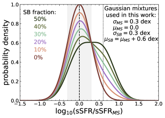
| Star-Forming Main Sequence | Speagle et al. (2014) | 2.3 | For the slope, we sample a Gaussian with and . We keep the time evolution components (Eqn. 28, therein), employing Gaussians for the parameters related to time. The starburst region is fixed to 0.6 dex above the main-sequence at a given stellar mass. We fix dex. |
| Main Sequence vs. Starburst Decomposition | \al@sargent12,dacunha15, sch15, michalowski17, popesso19, bisigello18, dudz20; \al@sargent12,dacunha15, sch15, michalowski17, popesso19, bisigello18, dudz20; \al@sargent12,dacunha15, sch15, michalowski17, popesso19, bisigello18, dudz20; \al@sargent12,dacunha15, sch15, michalowski17, popesso19, bisigello18, dudz20; \al@sargent12,dacunha15, sch15, michalowski17, popesso19, bisigello18, dudz20; \al@sargent12,dacunha15, sch15, michalowski17, popesso19, bisigello18, dudz20; \al@sargent12,dacunha15, sch15, michalowski17, popesso19, bisigello18, dudz20 | 2.3.1 | We step through six double Gaussian distributions, each with one mean centered on the main sequence and the other centered on the starburst regime ( dex). The distributions match the following starburst fractions: 50, 40, 30, 20, 10, and 0%. |
2.1 The Infrared Luminosity Function
We seed our model by generating mock populations of IR luminous galaxies according to the IR luminosity function (IRLF), with the structure described by Casey et al. (2018a, b) and updated parameters measured in Zavala et al. (2021). This IRLF is empirically-constrained at by well-known DSFG spectral energy distributions and physical properties derived using Spitzer and Herschel data (Casey et al., 2018b), and at using ALMA observations (Zavala et al., 2021). Below, we briefly describe the IRLF parameterization and constraints used in this work, and refer the reader to Casey et al. (2018b, a) for more details.
The IRLF in this model takes the form of a double power-law such that:
| (1) |
where (in L⊙) represents the evolving characteristic ‘knee’ of the luminosity function, represents the faint-end slope of the IRLF (below ), represents the bright-end slope of the IRLF (above ), and (in Mpc-3 dex-1) represents the evolving characteristic number density of the luminosity function.
Both L⋆ and evolve with redshift, reaching a “turning point” at (corresponding to the peak of the CSFRD) such that, at , L⋆ and evolve with a different slope than at . In other words, L⋆ and evolve as and , respectively, with and changing values at .
In general, the parameters describing the IRLF at are observationally well-constrained. We use the values listed in Table 3 of Casey et al. (2018b), with the exception of at for which we use the value measured in Zavala et al. (2021), and refer the reader to these works for more details on how these values were determined. Specifically, we fix the bright-end slope to , the redshift evolution of L⋆ to , and the redshift evolution of to . Together, these values successfully reproduce the measured IRLF, L⋆, , and the IR luminous galaxy contributions to the CSFRD at (see Appendix A.1 in Casey et al., 2018b).
At , there is much less information on the evolution of L⋆ and . For L⋆, studies report values as steep as (Gruppioni et al., 2013) and as flat as (Koprowski et al., 2017); this IRLF assumes a redshift evolution of , which is in line with the assumption that L⋆ evolves towards brighter luminosities at higher redshifts – as seen in several observational studies (e.g. Gruppioni et al., 2013; Koprowski et al., 2017; Lim et al., 2020). Higher values (e.g. ) would create unphysically bright IR luminous galaxies at that are not known to exist.
For the evolution of beyond , studies report values from (Koprowski et al., 2017) to (Lim et al., 2020), where more positive values correspond to a dust-rich early Universe, and more negative values correspond to a dust-poor early Universe. In other words, a dust-poor early Universe would manifest as a CSFRD that is not dominated by obscured star formation at , and there would be significantly fewer DSFGs in blank-field sub-mm surveys than there are at . In this work, we adopt the value presented in Zavala et al. (2021) where , corresponding to a more dust-poor early Universe. This value reproduces the most recent ALMA number counts at 1, 2, and 3 mm, as well as number counts from single dish telescopes at 700 m 1.1 mm.
The average faint-end slope collated in Casey et al. (2018b) is . However, recent works suggest a potentially shallower slope of (Zavala et al., 2018; Koprowski et al., 2017; Gruppioni et al., 2020; Lim et al., 2020; Zavala et al., 2021). For this work, we adopt the value reported in Zavala et al. (2021) where ; this value is aligned with the best fit faint-end slopes in Koprowski et al. (2017), Zavala et al. (2018), and Lim et al. (2020).
For this analysis, we randomly sample the parameter space for and as listed above and defined in Zavala et al. (2021). The parameters are modeled as skewed Gaussians, with values drawn for every realization.
In review, for each of the 103 model realizations (i.e. 103 lightcones), we randomly sample IRLF parameter values from their aforementioned distributions, then use the IRLF to generate a mock IR luminous galaxy population. To determine the number of IR luminous galaxies in a light cone slice (), we integrate the IRLF over bins of width L dex down to an IR luminosity of L⊙. To assign IR luminosities in a way that accurately reflects the shape of the IRLF, we then use the IRLF to generate a cumulative distribution function (CDF) for the respective LIR bin. Then, we draw galaxies from a random uniform distribution applied to the CDF ordinate. We use the randomly generated IR luminosities to calculate corresponding star formation rates according to Equation 12 in Kennicutt & Evans (2012, originally derived in ) using the variables listed in Table 1 therein for a total IR (TIR) to SFR conversion. We note that not all IR luminosity in a DSFG can be attributed to star-forming processes; some likely hails from AGN accretion activity. In the following section, we detail how we model potential AGN hosts and adjust their IR luminosities accordingly.
2.2 AGN Contributions to Total Infrared Luminosity
The integrated IR luminosity of galaxies encapsulates dust emission heated by both star formation activity and active black hole growth (i.e. active galactic nuclei, or AGN). Young stars embedded in dusty nebulae emit primarily UV and optical light that’s absorbed by the enshrouding dust. This warmed dust re-emits in the infrared spectrum. Similarly, actively growing coeval black holes are often surrounded by obscuring clumps of dust and gas that’s heated by high energy X-ray, UV, and optical photons, and also re-emits in the infrared. Theoretical and observational studies show that the bright end of the IRLF (L L⊙, depending on the epoch) is likely dominated by AGN-powered IR emission (Hopkins et al., 2010; Fu et al., 2010; Gruppioni et al., 2013; Symeonidis & Page, 2018, 2021), though AGN-driven IR emission is probably only significant at rest-frame m wavelengths (Brown et al., 2019). Similarly, studies on samples of IR luminous galaxies demonstrate that the higher the LIR, the more likely an AGN is present (Kartaltepe et al., 2010; Juneau et al., 2013; Lemaux et al., 2014) – with an occurrence rate of at L L⊙ at . Together, these lines of evidence indicate that we cannot assume that all IR emission from our mock galaxies hails only from star formation processes. Since we wish to use IR luminosity as an indicator for star-formation activity, we must correct for AGN contamination in the total infrared spectrum ( m).
To create a realistic correction effect, we must first define what fraction of IR luminous galaxies likely host an active supermassive black hole (regardless of how IR luminous the AGN is). For this step, we use the AGN population fraction in 70m bright sources as a function of IR luminosity reported in (Kartaltepe et al., 2010, Fig. 30 therein). This analysis included AGN selected through a myriad of techniques – X-ray detections, radio loudness, IRAC colors, and mid-IR power laws. At IR luminosities L⊙, less than 20% of the IR luminous galaxies host significantly bright AGN; but between L⊙, the occurrence rate of AGN jumps from 60% to nearly 100%. We note that other, more recent studies on AGN-SF host galaxy fractions report smaller AGN occurrence rates as a function of IR luminosity (e.g. Lemaux et al., 2014; Symeonidis & Page, 2021). Since we’re using total IR luminosity as an indicator for star-formation, which in turn will be used to later derive stellar masses (see Section 2.3), smaller AGN occurrence rates will result in larger stellar masses in this model. Thus, by using the larger AGN population fractions in Kartaltepe et al. (2010), we are choosing a more conservative approach that is less likely to predict an unphysical overabundance of massive star-forming galaxies.
After selecting a subset of mock IR luminous galaxies to host AGN, we must then decide exactly how much of the IR radiation comes from the AGN. For this step, we use the detailed analysis reporting mid and total IR contributions by AGN in ULIRGs at by Kirkpatrick et al. (2015). We use the distribution of mid-IR fractions (determined by Spitzer IRS mid-IR spectral decomposition, Fig. 3 therein) for designated composite and AGN-dominated galaxies as a probability distribution, and draw from this probability distribution to assign mid-IR AGN fractions to AGN hosts. Then, we use the quadratic relationship between mid-IR AGN fractions and total-IR AGN fractions to determine what percent of the total IR emission can be assigned to star formation (Equation 5 and Fig 14, therein). The majority () of AGN hosts in Kirkpatrick et al. (2015) exhibit mid-IR spectral features indicative of AGN mid-IR dominance (where f); it is only at this mid-IR fraction that AGN contamination to the total IR luminosity ( m) becomes significant ().
In general, this procedure has the most significant impact on our most luminous galaxies of L L⊙ – which often correspond to the most massive galaxies – with an average AGN total IR fraction of %. Note that the Kirkpatrick et al. (2015) relationship between mid-IR and total IR AGN dominance maxes out at f, corresponding to f. Some studies argue that AGN can be powerful enough to dominate the entire IR spectrum (e.g. Tsai et al., 2015; Symeonidis et al., 2016; Symeonidis & Page, 2018) while other studies argue AGN contributions are predominantly limited to the mid-IR (e.g. Brown et al., 2019). Additionally, recent results demonstrate the existence of a population of moderate to powerful AGN which were previously missing from these major AGN-galaxy co-evolution studies as they were assumed to be weak AGN but are instead likely heavily obscured (Lambrides et al., 2020). Together, these studies indicate that the true underlying relationship between galaxy IR luminosities and AGN processes is still unknown.
In summation, we use a suite of simple assumptions from the combined works of Kartaltepe et al. (2010) and Kirkpatrick et al. (2015) to correct a modest fraction of IR luminosities under the assumption that the IR emission is significantly powered by an AGN. These corrected IR luminosities are then used to calculate star formation rates (as detailed at the end of Section 2.1). In future work, we will explore more detailed treatments and characterization of AGN in massive dusty galaxies – and the consequences of these treatments and assumptions – in the context of this model.
2.3 The Star-Forming Main Sequence
One of the most ubiquitous and well-studied relationships describing galaxy evolution is the correlation between a galaxy’s star formation rate and stellar mass. This tight relationship, known as the star-forming main sequence (SFMS), suggests that most star-forming galaxies sustain steady (i.e. non-bursty) SFRs over several billion years (Noeske et al., 2007a, b; Daddi et al., 2007), at the end of which a galaxy exhausts its gas supply and moves off the main sequence towards quiescence. The correlation exists unambiguously across several orders of magnitude in stellar mass throughout cosmic time – from (e.g. Leroy et al., 2019; Popesso et al., 2019b) to as high as (e.g. Schreiber et al., 2017; Santini et al., 2017; Pearson et al., 2018; Thorne et al., 2021), theoretically making the SFMS useful in predicting stellar masses for a population galaxies with known SFRs, or vice versa.
The exact shape of the SF main sequence and its evolution through time is still the subject of intense debate. There is general agreement that the MS takes the form of a power-law (i.e. SFR M) with a tight intrinsic scatter of dex at M M⊙ (e.g. Speagle et al., 2014; Schreiber et al., 2015; Matthee & Schaye, 2019). In this same stellar mass regime, recent studies report that the SFMS slope, , lies between (e.g. Speagle et al., 2014; Lee et al., 2015; Schreiber et al., 2015; Tomczak et al., 2016). However, there is less consensus for galaxies with stellar masses M⊙ – which is the range of stellar mass we are primarily interested in for this work.
Several studies describe a flattening of the main sequence above a certain “turnover” mass, typically reported at M⊙ with possible evolution towards higher values during earlier times (e.g. Whitaker et al., 2014; Tasca et al., 2015; Schreiber et al., 2015; Lee et al., 2015; Tomczak et al., 2016). Above this mass, the main sequence is typically parameterized as a power law with a slope that is more shallow than the slope in the low-mass regime, effectively saturating in SFRs at high stellar mass. This bending could be driven by physical phenomena such as star formation suppression at high-masses or increased bulge contributions (e.g. Whitaker et al., 2015; Pan et al., 2017; Leslie et al., 2020; Thorne et al., 2021), and/or by observational effects such as contamination by passive galaxies (e.g. Johnston et al., 2015), biased/incomplete SFR indicators (e.g. Dunlop et al., 2017), or biased/incomplete SF galaxy sample selection techniques (e.g. Rodighiero et al., 2014).
For this work, we assume that the turnover at high masses is driven by observational effects, and that the true SFMS is a singular power law. The majority of studies reporting a high mass turnover selected their star-forming galaxy samples using optical / near-IR color cuts (Whitaker et al., 2014; Schreiber et al., 2015; Lee et al., 2015; Tomczak et al., 2016), such as the UVJ technique (Wuyts et al., 2007; Whitaker et al., 2011). However, color diagnostics centered in the ultraviolet to near-IR regime, while often the best available tool for such studies, are imperfect identifiers of dust obscured star-forming galaxies. Depending on colors and sample characteristics, anywhere from 5-50% of M dust obscured galaxies could be misclassified as quiescent due to their dust-reddened spectra (Schreiber et al., 2015; Domínguez Sánchez et al., 2016; Patil et al., 2019; Santini et al., 2019; Popesso et al., 2019a; Hwang et al., 2021). This misclassification effectively removes some of the most dust obscured, and therefore star-forming, massive galaxies from the analysis, whose SFRs would likely increase the high-mass SFMS slope. Furthermore, the high mass slope can also be analytically flattened by the misclassification of passive galaxies as star-forming (Johnston et al., 2015).
We note that if we do include a turnover component, extremely IR luminous galaxies in this model will scatter to unphysically high stellar masses ( M⊙). As described later in this section, we use IR-derived SFRs to pivot over the SF main sequence to assign stellar mass. A more IR luminous galaxy translates to a more star forming galaxy, which translates (generally) to a more massive galaxy. However, with the turnover, which is typically placed around M M⊙ and essentially flattens out from there, most galaxies at and beyond ULIRG luminosities (L L⊙) have SFRs beyond the SFR that corresponds to the turnover mass. In other words, the SFRs exhibited by some of the most extreme DSFGs are well beyond the turnover SFR that corresponds to the turnover mass and therefore have no “anchor” to pivot over. Thus, in this model, employing a turnover would require forcing highly star forming DSFGs to scatter around the asymptotic turn over and thereby generate an unphysically abundant population of incredibly massive galaxies.
Studies that sought specifically to constrain the stellar properties of DSFGs find these galaxies sitting on or above a proportionately more massive and more star-forming extension of a singular power law SFMS (e.g. da Cunha et al., 2015; Martis et al., 2016; Michałowski et al., 2017; Pearson et al., 2018). Recently, a growing body of literature is starting to establish the existence of massive, optically-dark dust obscured galaxy populations that were previously undetected in deep UV/optical/near-IR surveys (e.g. Spitler et al., 2014; Wang et al., 2019; Casey et al., 2019a; Williams et al., 2019; Toba et al., 2020; Smail et al., 2021; Manning et al., 2022) – the same surveys used to establish a global SFMS. It is therefore likely that the true underlying SFMS – one that includes massive dust obscured galaxies – takes the form of a power law all the way through the high stellar mass regime.
For this analysis, we randomly sample the power law slope of the SFMS from a Gaussian distribution centered at with a dispersion of . Using these slopes as opposed to more shallow ones is a more conservative approach; since we pivot SFRs over the main-sequence power law to derive stellar masses, employing shallower slopes (e.g. ) generates large, unphysical excesses of massive dust-obscured galaxies. Furthermore, this approach allows us to marginalize our results over the different competing MS slopes established in more recent literature (e.g. Schreiber et al., 2015; Lee et al., 2015; Tomczak et al., 2016; Bisigello et al., 2018). We use the evolving normalization () from the Speagle et al. (2014) SFMS (Equation 28, therein); this form is generally consistent across several studies using different populations of galaxies to determine SFMS properties (e.g. Johnston et al., 2015; Schreiber et al., 2015; Tomczak et al., 2016; Kurczynski et al., 2016; Pearson et al., 2018; Popesso et al., 2019a).
2.3.1 Main Sequence vs. Starburst Decomposition
In order to derive stellar masses for our mock IR luminous galaxies, we distribute them over the star-forming main-sequence space. However, there is currently no consensus on exactly where DSFGs as a population lie in main-sequence space. Some studies suggest these objects are primarily starburst galaxies, sitting 4 above the main-sequence at a given stellar mass, with such extreme SFRs driven potentially by mergers (e.g. Daddi et al., 2010; Hainline et al., 2011; Lee et al., 2013; Magnelli et al., 2014). In this work, we adopt the same starburst galaxy definition.111The traditional definition of starburst galaxies was based not on their distance from the SFMS, but on their rates of gas consumption (i.e. M/SFR, also known as the integrated Kennicutt-Schmidt relationship or star formation efficiency, e.g. Sargent et al. 2014). For the purposes of this paper, we use the distance to the main-sequence as the definition. As a whole, the starburst population is a relatively small portion of the overall star-forming galaxy population (e.g. at Sargent et al., 2012; Schreiber et al., 2015; Bisigello et al., 2018; Popesso et al., 2019a), but DSFGs are sometimes believed to be a ‘starburst-dominated’ sub-population of galaxies. Starburst-dominated populations could stem from sensitivity limits by the same surveys, where only the most extreme sources at will be detected. Such a designation is likely also driven by catastrophic projection / blending effects stemming from the large angular resolutions in most canonical wide-field sub-mm surveys built by both space-based (e.g. Herschel, Béthermin et al., 2017) and ground-based telescopes (e.g. SCUBA, Cowley et al., 2015).
Recent studies with better angular resolutions (using e.g. ALMA) reveal that significant percentages (50-100%) of DSFGs are proportionately more massive and star-forming extensions of coeval main-sequence galaxies (da Cunha et al., 2015; Michałowski et al., 2017; Wang et al., 2019; Dudzevičiūtė et al., 2020). This fraction may evolve with redshift, as shown in da Cunha et al. (2015) and Michałowski et al. (2017), but to generalize these fractions as evolutionary trends is problematic as they are dependent on the juxtaposed main-sequence parameterization and the far-IR / sub-mm selection limits; there is also a dearth of sufficiently large samples at epochs beyond to derive a statistically-relevant evolutionary picture. Thus, the true starburst fraction of DSFGs (at least the particularly massive and IR luminous ones) is still unknown, with the truth value likely lying somewhere in between .
Instead of forcing a singular underlying distribution as truth, we sample the model over several steps within the observed 50-100% range. Specifically, our model steps through DSFGs-as-starburst fractions of 0, 10, 20, 30, 40, and 50%, with the remainder belonging to the main-sequence regime. The distribution is modeled as a double Gaussian over main-sequence space, with one Gaussian centered over the main-sequence and the other centered dex away ( above the main-sequence, Rodighiero et al., 2011). Both distributions have fixed width of dex, similar to those measured in many main-sequence studies (e.g. Speagle et al., 2014). We tested the impact of these chosen widths by running the model with both smaller and larger dispersions ( and 0.4, respectively) and found no significant difference (%) in our results. These distributions are shown in Figure 2.
Similar to Section 2.1, we wish to randomly assign stellar masses in a way that accounts for Eddington bias: if we were to simply draw from the starburst vs. main-sequence Gaussian mixtures as a way to assign stellar mass, more numerous low star-forming galaxies would up-scatter into higher mass bins than high SFR galaxies into lower mass bins. Instead, we model the main-sequence vs. starburst mixtures as cumulative distribution functions, from which we sample a uniform distribution of stellar masses for our mock galaxy populations. This method ensures that galaxies with higher SFRs are more likely to have larger stellar masses, in alignment with observations.
2.4 Stellar Mass Space Density
After using the star-forming main-sequence to generate stellar masses for the mock IR luminous galaxies, we can then bin in stellar mass space to determine the three dimensional stellar mass space density. Galaxies are binned based on their stellar mass in bins of size dex – corresponding to the average spread in stellar mass in the SFMS (Speagle et al., 2014). The stellar mass histograms are then divided by the same respective light cone volumes used to generate mock galaxies from the IRLF.
3 The Dust-Obscured Stellar Mass Function
3.1 Model Fitting Procedure
To briefly review the model thus far (Sections 2.1 – 2.4): we use the IR luminosity function to generate a mock catalog of dust-obscured star-forming galaxies in a given redshift range over 1 deg2. Redshift bins (listed in Table 2) were designed to match SMF studies in the literature for ease in comparison. We correct the IR luminosities for AGN contributions, then convert the corrected IR luminosities to star formation rates. Then, we use the SFRs to pivot the mock galaxies over the star-forming main sequence to generate mock stellar masses. Finally, we bin the mock galaxies in stellar mass space and divide by the light cone volume to calculate stellar mass space densities across cosmic time (as a function of stellar mass).
This entire procedure is repeated 103 times: a thousand realizations for each of the six different main-sequence vs. starburst distributions (described in Section 2.3.1 and shown in Figure 2). Median values of the space densities within each of the six runs are calculated (across the abscissa, i.e. stellar mass bins), and uncertainties determined from the inner 68% confidence interval. This allows us to directly gauge the impact of varying main-sequence vs. starburst Gaussian mixtures on the resulting stellar mass function.
Then, within each of the six starburst vs. main-sequence mixtures and for each respective redshift window, we fit a broken power law to the stellar mass space densities. Historically, stellar mass functions are modeled as Schechter functions (Schechter, 1976), but the underlying distribution that our model draws from is a broken power law (the IRLF, Casey et al., 2018b). Still, we computed the Bayesian information criterion (Schwarz, 1978) to determine whether the Schechter function or a broken power law better models our resulting stellar mass function. The Bayesian information criterion (BIC) is a tool used to choose between two or more models, where models are penalized for the number of parameters included in the fit. A smaller BIC corresponds to the better fit, with a difference of BIC indicating a very strong case for the best model. Across all mixtures/redshifts, we found that the broken power law resulted in a stronger model (with BIC in nearly all cases). Thus, we adopt the broken power law form to define the number density of dust-obscured galaxies, , as:
| (2) |
where (in Mpc-3 dex-1) is the number density normalization, , is the low mass slope, M⋆ is the characteristic mass or ‘knee’ of the SMF, and is the high mass slope (beyond the knee). We visually inspect the stellar mass space densities in each mixture-redshift combination and find that the low-mass slope () and the characteristic mass (M⋆) do not significantly evolve across mixtures or redshifts ( difference between all mixture-redshift combinations). Therefore, to reduce the degrees of freedom, we fix and M M⊙ universally across all epochs/mixtures. Upon visual inspection, both of these values combined well-reproduced the low-mass regime of the DSFG stellar mass function for all mixture-redshift combinations. For posterity, we also tested a smaller M M⊙ and a steeper (more inline with UV/OP-based studies). This resulted in a difference in the derivations of and , the overall values were poorer, indicating preference for a more massive knee and shallower low-mass slope.
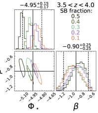
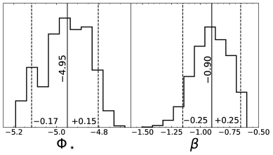
Then, still within the individual mixture-redshift combinations, we run 104 realizations of a Metropolis-Hastings (i.e. MCMC) algorithm to find the best-fit values for the number density normalization, , and massive-end slope, . We allow log10() to range between and between . The quality of each broken power law fit is determined by computing the chi-square goodness of fit against the mock stellar mass space densities; we only compute the using stellar mass space densities with 68% confidence intervals that are less than an order of magnitude away from the median value (i.e. log10() 1). This primarily affects the highest mass bins (M M⊙) where mock IR luminous galaxies appear rarely and therefore aren’t produced consistently in the model.
In Figure 3, we show the resulting constraints on and for an example redshift bin. There is some marginal covariance with starburst fraction and , such that increasing starburst fractions causes a smaller overall number density of massive IR luminous galaxies (as expected). However, the differences between across mixtures is small ( dex at most) and, moreover, the median in each mixture is captured within the final uncertainty derived for this redshift bin. Thus, this covariance is insignificant for the purposes of this work. Additionally, there is no clear trend between the high-mass slope and starburst fractions across all epochs. One might expect a shallower to arise from a smaller starburst fraction because with low starburst fractions more galaxies are deemed main-sequence-like and thus scatter to higher stellar masses; this effect in theory creates more numerous massive galaxies than model realizations with “high” starburst fractions, and causes the population density near/beyond M⋆ to increase. However, in this case, it’s likely that the most extreme IR luminous / dust-obscured star-forming galaxies are so rare that a consistently small population emerges at masses M⋆, regardless of the employed main-sequence vs. starburst mixture.
To derive a singular stellar mass function from the six different main-sequence vs. starburst mixtures, we randomly draw 103 pairs of (, ) from the converged MCMC chains of each mixture. We collate the 103 pairs of (, ) and determine the median and 68% confidence interval. This process is completed separately for each redshift window. We show example collated histograms for and in the redshift bin in Figure 3.
It is important to note that the main basis of this model hinges upon the accuracy of the modeled IR luminosity function. As reviewed in Section 2.1, the evolution of the IRLF beyond is still under debate (e.g. Gruppioni et al., 2020). While we marginalize over several parameters to account for these unknowns, there are still some fixed assumptions in this work, such as the evolution of L⋆ at , or the lackthereof for the faint-end slope, . We find that a steeper results in a less than difference in the final derivations of the parameters describing the dust-obscured SMF; and a flatter evolution of L⋆ with results in a less than difference in the resulting SMF parameters. Thus, to be conservative and account for the impacts of our model’s main assumptions, we add an additional 10% uncertainty on the ultimate stellar mass function parameters. This additional uncertainty is included in Figure 3 and in Table 2, where the ultimate SMF parameters for this analysis are listed.
| Dusty Star-Forming Galaxies | Quiescent Descendant Galaxies | |||||||
|---|---|---|---|---|---|---|---|---|
| Redshift | log) | log) | log) | log) | ||||
| 10.8 | 10.8 | |||||||
| 10.8 | 10.8 | |||||||
| 10.8 | 10.8 | |||||||
| 10.8 | 10.8 | |||||||
| 10.8 | 10.8 | |||||||
| 10.8 | 10.8 | |||||||
| 10.8 | 10.8 | |||||||
| 10.8 | 10.8 | |||||||
| 10.8 | 10.8 | |||||||
3.2 Comparison to Literature SMFs
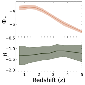
In Figure 4, we show the redshift evolution of and for our final dust-obscured SMF across time. The number density normalization stays relatively constant at log10(/(Mpc-3 dex-1)) in the 5 Gyr redshift window, but experiences nearly an order of magnitude increase in the 1.5 Gyr between and and a similar strength in growth in the 1 Gyr between and . This points to an era of rapid stellar mass growth in the Universe for massive dust-obscured galaxies that is unmatched at later times. Interestingly, however, we do not see any significant evolution in the massive end slope of the SMF, , which has an average value of across all epochs. Combined, the evolutionary properties for these two parameters paint a picture in line with the cosmic downsizing scenario, where the most massive star-forming galaxies built the majority of their stellar mass in the first 1-2 Gyr, and quench by . Furthermore, the rate of growth and quenching in dust-obscured galaxies must occur on short timescales (at least shorter than the 1 Gyr-wide redshift windows); in other words, if remains relatively stable across time, then dust-obscured galaxies likely grow into and then quench out of the massive end of the star-forming SMF at a nearly equivalent rate.
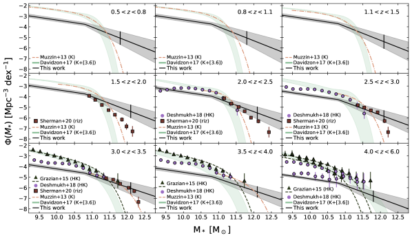
In Figure 5, we show the final star-forming stellar mass functions derived from IR luminous galaxies across . We remind the reader that the IRLF does not account for all star-forming galaxies and therefore agreement between res-frame UV/OP-based SMFs and the dust-obscured SMF generated in this work is not necessarily expected. Moreover, since our SMF takes a different functional form than those presented in the literature, we cannot quantitatively speak to differences in shape and parameterization. We can, however, discuss qualitative and integrated differences (the latter of which is discussed in detail in Sections 4.2 and beyond). Furthermore, due to the scientific purpose of this work, we focus the majority of this discussion to the more massive end of galaxy evolution at M M⊙, but show the less massive end of this and literature SMFs for the reader to understand the overall extrapolation of this model’s results to low masses.
In general, the dust-obscured SMF produced by this model is consistently below that of UV/OP-based predictions for star-forming galaxies at masses M⊙. It is around this mass that there appears to be a convergence between UV/OP and dusty SMFs, which then turns into a dust-obscured dominated stellar mass function at high masses. As mentioned before, this is likely because low mass galaxies are not accounted for in the IRLF as they are less obscured by dust. The discrepancies between the observed SMFs and our model are greatest at , where our model posits a significant population of M M⊙ galaxies while the UV/OP-based estimates see none (see Figure 6). At , our model shows some agreement with that of the -based SMF derived in Sherman et al. (2020). We believe this agreement to be artificial as it could be argued that there are high rates of AGN contamination in the Sherman et al. sample. This is because AGN are removed from this sample using SDSS data which likely does not sufficiently capture high redshift and/or obscured AGN. At , we also see some partial agreement between our model, the Muzzin et al. (2013) results, and the massive, dusty galaxy sample within Deshmukh et al. (2018) out to M M⊙. Both of these works select their galaxy samples using and/or -band images with observational depths near the limits of known massive, dust-obscured galaxies (e.g. Simpson et al., 2014; da Cunha et al., 2015; Cowie et al., 2018; Dudzevičiūtė et al., 2020), so it is likely some of the massive dust-obscured population is captured in these works. However, at these and -band depths, only % of dusty, star forming galaxies are typically detected, leaving a significant population of optically faint galaxies (also known as ‘OIR-dark’, Wang et al., 2019; Williams et al., 2019; Casey et al., 2019b; Manning et al., 2022) – that are likely some of the most massive and heavily dust obscured galaxies in the cosmos (Pannella et al., 2009; Dunlop et al., 2017; Whitaker et al., 2017; Fudamoto et al., 2020) – unaccounted for in the massive end of these stellar mass functions.
It is also interesting that our results are in more severe disagreement with the Davidzon et al. 2017 analysis as the authors introduce a deep Spitzer IRAC [3.6 m] image to help capture more dust-obscured and quiescent galaxies than the typical rest-frame UV/OP-selected SMFs. Yet, the Davidzon et al. SMF yields fewer star-forming galaxies beyond M M⊙ than any other SMF discussed in this section. This could be due to a variety of factors. For example, the Davidzon et al. work required detection in a combined image; the 3 detection limit of the reddest band (Ks = 24) could miss 40% or more of dusty galaxies due to their faintness (Simpson et al., 2014; Brisbin et al., 2017; Dudzevičiūtė et al., 2020). Another factor could be the fact that galaxy stellar masses were derived solely from rest-frame UV to optical wavelengths – no far-infrared (i.e. cold dust) information was included in SED fitting. If there is heavy obscuration of the stellar spectrum, and no energy coupling between optical/mid-IR and FIR observations, stellar masses can be underestimated by a factor of 23 due to faintness (Buat et al., 2019), and/or a mildly quiescent galaxy spectrum could be assumed (especially with limited photometry). Both of these employed methods can remove massive, dust-obscured galaxies from the massive end of the star-forming SMF.
At , the dust-obscured SMF is below UV/OP-based estimates at similar redshifts, except where they meet at the most massive point around M M⊙. While there is still large uncertainty in the prevalence of dust-obscured galaxies at (see e.g. Zavala et al. 2021, c.f. Gruppioni et al. 2020), it appears from this model and from UV/OP-based estimates that such massive galaxies are exceedingly rare at these epochs and their population density really begins to build after this epoch.
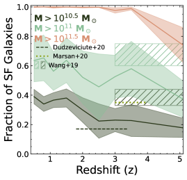
In Figure 6, we show the fraction of massive, dust-obscured galaxies among all star-forming galaxies using the Davidzon et al. (2017) SMF as a proxy for UV/OP-bright star-forming galaxies (i.e. the denominator is derived from Davidzon et al. plus the estimate from this work). We show that from dust-obscured galaxies become more prominent at higher stellar masses. Though there is large uncertainty, we predict that 20-40% of galaxies at M M⊙ are dust obscured, which is similar to the fraction of -band undetected SMGs in Dudzevičiūtė et al. (2020), the -band dropout sample in Wang et al. (2019), and the dust-reddened sample in Marsan et al. (2022). The percentage increases to 50-60% at M M⊙, and finally maxes out to nearly 100% at M M⊙. Interestingly, these results are in agreement with the Whitaker et al. (2017) study, which arrived at a dust-obscured fraction of massive galaxies using a completely different method – quantifying the fraction of dust-obscured versus UV/OP-bright star formation in individual massive star-forming galaxies at . At , we caution interpretation of the M M⊙ DSFG fractions as galaxies of this mass were so rare that they were not consistently produced in this model.
We note that there may be some massive DSFGs with sufficient escaping stellar emission to be captured in the UV/OP-based estimates and therefore there may be some “double counting” of massive SF galaxies in this space. Understanding the significance of that effect is beyond the scope of this paper, and likely unfeasible until sufficient wide-field JWST near-IR surveys are completed.
4 Number and Stellar Mass Densities
For the remainder of this work, we focused on the massive, dust obscured population of galaxies predicted by our model, defined as all objects with M M⊙ and L L⊙. We emphasize that the latter criterion emerged naturally in this model: nearly all () M M⊙ star-forming galaxies produced by our model, across the redshift space probed here, have LIRG or greater IR luminosities; moreover, of these massive star-forming galaxies have ultra-LIRG (ULIRG, L L⊙) luminosities or higher. We hereafter refer to these IR luminous massive galaxies as massive DSFGs.
4.1 Duty Cycle Correction
Gas depletion timescales measured in high- DSFGs suggest that the IR luminous phase of star formation is short lived (on the order of tens to a few hundred Myr, Tacconi et al., 2006; Barro et al., 2014; Aravena et al., 2016; Yang et al., 2017; D’Eugenio et al., 2020; Zavala et al., 2022). This means that massive DSFGs are only traceable via their incredible IR emission for a small window of time, and therefore IR / sub-mm surveys are likely incomplete in capturing the DSFG population over cosmic timescales significantly wider than a few hundred Myr. If we assume that massive DSFGs are the primary progenitor population to massive quiescent galaxies at later times, we can derive a “duty cycle correction factor” that forces the two population densities to match over respective redshift windows (as seen in e.g. Toft et al., 2014; Valentino et al., 2020).
We iteratively tested a range of duty cycles from 50-1000 Myr and found that a duty cycle correction factor of 500 Myr was most effective in matching our predicted number densities to those of massive quiescent galaxies observed in the literature. Duty cycles on the order of a few hundred Myr or less result in a significant over production (10 more) of observed quiescent descendants across all epochs, while cycles closer to 1 Gyr under produce the descendant population by 0.5 dex at . We note that a duty cycle correction of 500 Myr only significantly impacts model results at ; all results at remain roughly the same in both the pre- and post-duty cycle corrected model as the widths of the redshift windows are approximately equivalent to the duty cycle correction factor. We show the pre- and post-duty cycle correction model predictions in Figure 7 as purple and pink bands, respectively, and discuss further potential implications of this value in Section 5.2.
4.2 Massive DSFG Number Densities
In Figure 7, we show the redshift evolution of the number density of massive DSFGs (left), and of their quiescent descendants (right). During the Gyr between and 6, we predict an order of magnitude increase in number density of M M⊙ dust obscured SF galaxies, similar to that seen in Marsan et al. (2022). This growth rate tapers off at later times, taking another Gyr (from to 1.5) to achieve another order of magnitude of growth in population density. This evolution is steeper than that exhibited by UV/OP-based estimates from e.g. Davidzon et al. (2017), where it takes an additional half a billion years to achieve similar growth. In general, across , UV/OP-bright massive SF galaxies are more populous, except at where we find an order of magnitude more UV/OP-bright galaxies than massive DSFGs. (However, as shown in Section 3.2 and Figure 6, the overall fraction of massive DSFGs compared to UV/OP-bright galaxies is larger at higher stellar mass thresholds.)
One of the primary pieces of evidence that pins DSFGs as ancestors to giant ellipticals at later times is the similar co-moving number densities between the two populations (e.g. Toft et al., 2014). However, the strength of this evolutionary picture is discrepant depending on the sample size, depths, and sensitivities of far-IR and sub-mm surveys used to characterized the massive, dust-obscured population. For example, Herschel discovered DSFGs at are often comprised of a rare and extreme star-forming population (with SFRs up to and exceeding 1000 M⊙ yr-1); their number densities are insufficient to match those estimated for massive quiescent galaxies at (Dowell et al., 2014; Ivison et al., 2016; Duivenvoorden et al., 2018; Ma et al., 2019; Montaña et al., 2021). Instead, the recently discovered H-band dropouts, or alternatively the larger umbrella of galaxies that are optically “invisible” but sufficiently bright in the far-IR/sub-mm regime ( mJy), may make up the bulk of the massive, star-forming galaxy population at (Williams et al., 2019; Wang et al., 2019; Lagos et al., 2020; Manning et al., 2022). Thus, it is perhaps more important to successfully model these more common, less extreme dusty, star-forming galaxies.
At , when integrated over similar redshift ranges, our model successfully predicts similar space densities of the massive ( M⊙) submillimeter galaxy populations presented in Dudzevičiūtė et al. (2020, Mpc3 at ), but predicts more massive DSFGs than what is seen in the Michałowski et al. (2017) SCUBA-2-detected sample in a similar redshift range. This difference is likely due to the employed SFR cutoff in the latter work, which only includes galaxies with SFRs M⊙ yr-1. In our model, % of M M⊙ galaxies at have SFRs M⊙ yr-1 (with the percent decreasing with increasing redshift) – this difference in population properties is sufficient to match the gap between our results and those seen in Michałowski et al. (2017), within uncertainty.
At , the model’s success is difficult to quantify due to lack of strong observational constraints, including insufficient sample sizes of DSFGs and highly uncertain redshifts. Still, we find general agreement between the model and observations out to , though observational uncertainties span two orders of magnitude. At , the model predicts massive DSFG number densities in agreement (within uncertainty) with those of the Michałowski et al. (2017) sample (n Mpc3). At , we compare to the ALESS (da Cunha et al., 2015), COSMOS (Miettinen et al., 2017), and S2CLS (Michałowski et al., 2017) samples as calculated in Valentino et al. (2020, pre-duty cycle correction). To derive number densities for these surveys, Valentino et al. (2020) took strict photometric redshift constraints, requiring that both upper and lower limits on the photo-s sit at or above . As seen with the S2CLS derivations between Michałowski et al. (2017) and Valentino et al. (2020), this requirement can reduce the number densities by an entire order of magnitude, thereby demonstrating to first order one of the main difficulties in constraining DSFG number densities at . Across these three surveys with conservative photo- restrictions, our model estimates lie between those derived from the COSMOS Miettinen et al. (2017) and ALESS da Cunha et al. (2015) samples, where n Mpc3 at , which is also roughly in alignment with Michałowski et al. (2017).
Comparing to the observed number densities of the (potentially more populous) optically dark dust-obscured galaxies at is particularly difficult as observational constraints suffer either from small sample sizes (n , e.g. Williams et al. 2019; Manning et al. 2022), or are averaged over extremely large redshift ranges (e.g. in Wang et al. 2019). When comparing to estimates derived from a single exceptional object in Williams et al. 2019, our model predicts nearly 30 smaller populations of massive DSFGs. While the Wang et al. 2019 sample of H-band dropouts includes a larger sample size () over a larger survey area (600 arcmin2), these objects span a (photometric redshift) range of , with over half of the sample exhibiting redshift errors . Still, when integrating our model across , we find a similar space density as the authors (reported as n Mpc3) as well as the entire sample of 2 mm detected galaxies in Manning et al. (2022). When including only galaxies with redshifts estimated at , both the Wang et al. and Manning et al. estimates drop to n Mpc3, which is closer to our model predictions. Unfortunately, due to the large uncertainties in the observational data, we limit and conclude our interpretation of the discrepancies between this work and the aforementioned optically-dim sources until further, more robust surveys are completed.
4.3 Quiescent Descendants
4.3.1 Generating Quiescent Descendants
The discovery and follow up observations of massive galaxies within the first 1-2 Gyr of the Universe suggest that they form via extremely efficient and rapid star formation mechanisms during the early cosmos (e.g. Glazebrook et al., 2017; Schreiber et al., 2018a, b; Marsan et al., 2022; D’Eugenio et al., 2020; Valentino et al., 2020). This is likely in the form of bursts of extreme star formation ( M⊙ yr-1) lasting Myr (e.g. Tacconi et al., 2006; Barro et al., 2014; Aravena et al., 2016; Yang et al., 2017; D’Eugenio et al., 2020; Zavala et al., 2022), after which the cold gas reservoir is depleted, heated, and/or blown out.
In our model, we make the following simplistic assumptions to derive descendant quiescent galaxy masses to compare with observations and models in the literature. We assume that the current SFR of a mock galaxy is maintained for an additional Myr, in alignment with the gas depletion timescales seen in the aforementioned observational studies. These timescales are randomly sampled from a uniform grid with steps of Myr. Then, we forward evolve the galaxy, adding the additional stellar mass built assuming a continuous SFR over the given timescale; to determine the redshift of the ‘quenched’ galaxy, we add the same timescale to the galaxy’s star-forming redshift (which was assigned in the initial model).
There are caveats to our simple forward evolution model: we do not include any prescriptions for AGN feedback, merging activity, additional gas accretion, or any other potential phenomenon that could theoretically slow down or speed up the SFRs / gas depletion timescales assigned to our mock galaxies. We see this as a strength of this model: there is no need to invoke complex assumptions on e.g. available gas mass reservoirs and potential heating mechanisms in order to successfully reproduce observed massive galaxy population densities (as shown in the proceeding Section). Furthermore, it is entirely possible that these more second-order corrections can be accounted for in the marginalization / uncertainty propagation process. For example, minor bumps or dips in the IRLF due to major mergers triggering IR-luminous star-formation would be accounted for in the uncertainty in the IRLF parameter space. Thus, while a more sophisticated model may be more “complete” in it’s physical assumptions, it does not appear necessary to describe massive galaxy evolution to a first-order approximation.
4.3.2 Quiescent Descendant Densities
On the right panel of Figure 7, we show the expected evolution in the number density of massive DSFG quiescent descendants derived in Section 4.3.1. In general, this model does an excellent job at modeling observed number counts in heterogeneous samples of massive, passive galaxies across (Muzzin et al., 2013; Toft et al., 2014; Straatman et al., 2014; Davidzon et al., 2017; Schreiber et al., 2018a; Merlin et al., 2019; Santini et al., 2019; Shahidi et al., 2020; Carnall et al., 2020). This is particularly promising because of the heterogeneity across these samples: each of the aforementioned bodies of work has their own methods/thresholds of selection and characterization of passive galaxies, yet we are able to successfully reproduce similar estimates across such diversity. Some have slightly lower stellar mass thresholds (e.g. M M⊙, Shahidi et al., 2020; Carnall et al., 2020), or are only complete at higher stellar masses than those explored in this work (e.g. M M⊙ at , Muzzin et al., 2013). Some employ specific SFR (sSFR SFR/M⋆) cuts that capture post-starbursts (e.g. log(sSFR/yr) , Straatman et al., 2014), which are likely more in line with our model’s assumptions / definition of massive DSFG descendants, while others focus strictly on fully quiescent galaxies (e.g. log(sSFR/yr) , Davidzon et al., 2017).
Our model most disagrees with the work of Girelli et al. 2019, where we predict nearly an order of magnitude more passive galaxies at . While Girelli et al. place similar stellar mass and sSFR cuts on their sample as some of the aforementioned studies, their quiescent galaxy selection technique is unique. They develop a color selection criteria based on mock quiescent galaxy colors generated from stellar population synthesis models. They employ an exponentially declining star formation history with a short -folding time (100-300 Myr) such that the galaxies are quiescent at the time of observation (1-2 Gyr into the Universe). In effect, this could mean that post-starburst galaxies are not captured in this color space as their colors are likely bluer than the objects discovered in Girelli et al. As mentioned before, it is likely that our model quiescent descendants fall in the post-starburst category, and therefore would be missed in the Girelli et al. study, possibly accounting for such a discrepancy in number densities.
Like the ancestral massive DSFG population, this model predicts an order of magnitude increase in the number density of passive galaxies from to 3 (i.e. over Gyr), a growth rate similar to that seen in Santini et al. 2019 and Merlin et al. 2019, and another order of magnitude over nearly twice the amount of time from to 1.5. This is unsurprising given the relatively short gas-to-stars duty cycles used in this work and exhibited by DSFGs at high redshifts (e.g. Tacconi et al., 2006; Aravena et al., 2016).
4.4 Comparison to Models
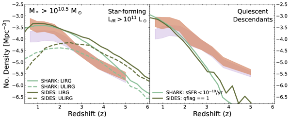
In Figure 8, we compare our results to other models relevant to this work as evident by their established success in reproducing properties and/or observations of submillimeter-bright galaxies. First is the Shark semi-analytical model (Lagos et al., 2018, 2020), which well-reproduced on-sky number counts at m mm across . Shark is a physical model that follows the formation of galaxies in a CDM universe using a large suite of physical models for e.g. star formation, as well as stellar and AGN feedback. We also emply the Simulated Infrared Dusty Extragalactic Sky (SIDES) empirical model (Béthermin et al., 2017), which is successful in reproducing number on-sky counts of single-dish (i.e. confusion-limited) instruments, e.g. Herschel PACS and SPIRE observations at m. SIDES was built using compiled observational results on the SFMS and stellar-to-halo mass relationships.
To compare the SIDES model, we use the publicly available catalogs,222SIDES catalogs can be found here: http://cesam.lam.fr/sides. taking all galaxies with stellar mass M⊙ in the same redshift bins as defined in Table 3. We use the passive galaxies flag (qflag == 1) to separate star-forming and quiescent galaxies, and further divide the star-forming sample into LIRGs and ULIRGs (L L⊙) by converting the provided SFRs into IR luminosities using the same conversion employed in our model (Murphy et al. 2011; Kennicutt & Evans 2012, see Section 2.1). To pull an analogous massive DSFG population from the SHARK model (C. Lagos, priv. communication), we use the same stellar mass, redshift, and IR luminosity criteria; for a comparative quiescent galaxy sample, we include post-starburst / near-quenching galaxies in the SHARK passive galaxy sample, defined as galaxies with log(sSFR/yr) . Galaxy properties (i.e. SFR and stellar mass) in both populations were convolved with random Gaussian noise of width 0.2 dex prior to calculating number and stellar mass densities.
At , our (duty-corrected) model is in agreement with the massive LIRG (aka massive DSFG) estimates in both SHARK and SIDES. Beyond this redshift, the SIDES model predicts roughly three times as many massive DSFGs at all epochs, while the SHARK model predicts only twice as many up until when our results drop back into alignment.
While all mock massive DSFGs in this work have IR luminosities of LIRG status or brighter across , the majority (75-99%) of massive DSFGs exhibit even brighter ULIRG-like luminosities at . Thus, a more appropriate population comparison might be the ULIRG population in both the SIDES and SHARK models. Indeed, when comparing to the ULIRG population in both models, our results are significantly less discrepant, with a near-perfect agreement in predictions from the SHARK massive ULIRG model population at . Consistency across the SHARK model and this work may be due to their careful and considerate treatment in relating dust surface densities with attenuation in the stellar continuum, including an energy balance in the far-infrared. One potential reason that the SIDES model, which is empirically-based and similar in build to this work, produces a higher density of massive IR luminous galaxies is due to differing star formation rate calculations. In SIDES, LIR is converted to SFR using the Kennicutt 1998 equation, while in this work we use the relationship from Kennicutt & Evans 2012, which produces SFRs roughly 24% lower than the former. We tested our model using the same LIR-to-SFR conversion as in SIDES and found that this SFR prescription brings our models into agreement for the massive ULIRG population, but our quiescent descendant population is overproduced by up to 0.5 dex when compared to observations.
As shown on the right side of Figure 8, both the SIDES and SHARK models produce significantly fewer massive quiescent galaxies at than this model. The SIDES team used SMF results from Davidzon et al. 2017 to populate their model; this limits their model quiescent sample to strictly passive galaxies (log10(sSFR/yr) ), while many of our model quiescent descendants are more likely post-starbursts (log10(sSFR/yr) ). Thus, it is unsurprising that the SIDES quiescent number densities, like those reported in Davidzon et al. 2017, are up to a decade lesser in population density than our model predicts at . For the SHARK model, we capture post-starburst and strictly passive galaxies, yet see predictions as discrepant as those in the SIDES model. The massive end of the total galaxy SMF in SHARK appears most sensitive to AGN feedback efficiency, but it is unclear if weaker AGN feedback would (or would not) produce sufficient populations of massive quiescent galaxies to match our predictions at earlier times.
| Massive DSFGs | Quiescent Descendants | |||
|---|---|---|---|---|
| Redshift | log10(n) | log) | log10(n) | log) |
| -3.37 | 7.23 | -3.23 | 7.28 | |
| -3.49 | 7.25 | -3.32 | 7.35 | |
| -3.48 | 7.30 | -3.26 | 7.45 | |
| -3.60 | 7.29 | -3.37 | 7.44 | |
| -3.97 | 7.13 | -3.84 | 7.31 | |
| -4.42 | 6.81 | -4.26 | 6.95 | |
| -4.75 | 6.58 | -4.60 | 6.64 | |
| -5.07 | 6.26 | -5.07 | 6.27 | |
| -5.62 | 5.53 | -5.43 | 5.95 | |
4.5 Stellar Mass Density
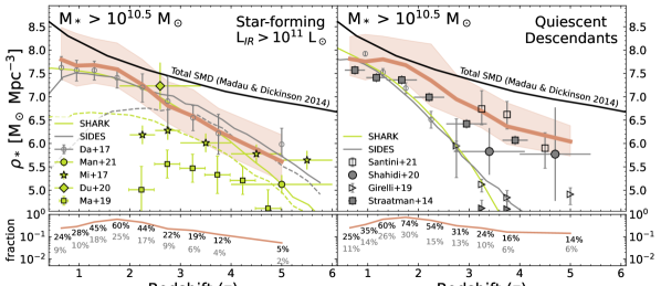
Cosmic volume averaged studies over the last decade show how instrumental the dusty, star-forming galaxy population is in understanding stellar mass build up over cosmic time: their intense dust-obscured star formation rates dominate over unobscured (UV/OP-bright) star formation at (Madau & Dickinson, 2014; Casey et al., 2014; Zavala et al., 2021). However, the integrated cosmic star formation rate density (cSFRD) appears roughly 2 ( dex) greater than the measured cosmic stellar mass density out to (Madau & Dickinson, 2014; Leja et al., 2015), indicating an issue with ‘missing’ stellar mass in direct measurements. Most of the potential explored drivers of this discrepancy are systemics such as overestimated star formation rates (Tomczak et al., 2016), underestimated stellar masses due to inflexible SED analysis (Leja et al., 2015, 2020), and photometry limitations (Madau & Dickinson, 2014). Missing from this conversation is a potential key component: it’s the incomplete accounting of stellar mass from the massive dust-obscured population (see Ma et al. 2019 for one of the only attempts). Owing to their heavily obscured nature, the field is still lacking in sufficient stellar continua observations for complete samples of DSFGs. One may argue that DSFGs are extremely rare and therefore not as significant in this discussion; however, as shown by the cSFRD, extreme properties of rare galaxies can be major – or even dominant – contributors when computing cosmic volume averaged quantities.
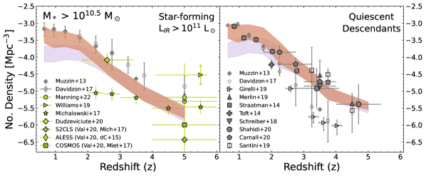
In Figure 9, we show the predicted contributions of massive DSFGs and their descendants to the cosmic stellar mass density (SMD). At , this model predicts that massive DSFGs hold from one tenth to a quarter of the total SMD derived from the integrated cSFRD (Madau & Dickinson, 2014). This fraction increases to a peak around , where massive DSFGs may contribute as much as 60% of the SMD (and as little as 25%). Such high fractions translate to a dex increase on the observed SMD, which would be sufficient to bring the observed and integrated SMDs into alignment. Beyond , the fraction steadily declines to at , demonstrating how this population is likely less significant in cosmic volume studies in the high- Universe (possibly because this population may still be growing to sufficient sizes during these epochs). We see a similar rise and fall in the quiescent descendant population, reaching a maximum fraction of at .
When compared to other studies, we predict that the massive dust-obscured population is an equally important contributor to the SMD as the massive UV/OP-bright star forming galaxies captured in (Davidzon et al., 2017). Furthermore, this model is in rough agreement with the handful of existing constraints on observed massive DSFGs (e.g. Michałowski et al., 2017; Dudzevičiūtė et al., 2020; Manning et al., 2022), with the exception of Ma et al. (2019) which probes a much more extreme and rare sub-population of massive DSFGs. We find that the lower SMD estimates of our quiescent descendant population is very similar to the Straatman et al. 2014 ZFOURGE mass-limited (M M⊙) sample, while our median prediction is in more agreement with Santini et al. 2019. Interestingly, our model results agree most with SMD predictions for the massive LIRG population in both the SIDES and SHARK models, whereas our predicted number density evolution was more in line with massive ULIRGs in both simulations. This likely means that the intrinsic stellar mass distributions in our model are skewed higher. In other words, the difference in SMDs is likely driven not by the number density evolution () but by the shape of the high-mass end of the stellar mass function; our shallow broken power law extension beyond the knee likely yields a higher abundance of extremely massive galaxies.
5 Other Model Implications
5.1 AGN LIR Correction Is Necessary
In Section 2.2, we described how we corrected the mock galaxies’ IR luminosities for AGN contamination so we could use LIR to derive star formation rates, which were in turn used to derive stellar masses (via distributing SFRs over the star-forming main sequence). We tested the model results without the AGN correction procedure and found that the resulting SMF parameters change by an average of . While seemingly insignificant, this propagates into an overestimate of the number density of massive DSFGs and their descendants by roughly half a dex at . This is particularly relevant for studies with galaxy populations selected via IR emission at m wavelengths without sufficient multi-wavelength data to rule out major AGN contributions between m. For these studies, it is possible that some of the selected galaxies have IR luminosities driven by AGN heating rather than by star-formation (Ciesla et al., 2015).
5.2 The Duty Cycle & Multiple Star Formation Bursts
In Section 4.3.1, we discuss how we create the mock quiescent descendant population by sampling gas depletion timescales of Myr, and in Section 4.1, we discuss how we correct the model number densities to match observed number counts using a duty cycle correction factor of 500 Myr. Why don’t these values match?
The range of gas depletion timescales used in this work are derived from direct measurements in the literature. They are generated using a closed-box assumption such that given a galaxy’s measured SFR and molecular gas mass, one can compute how long the galaxy could sustain such a star formation rate before depleting it’s molecular gas reservoir. Yet, observations and simulations show that the star formation history of massive DSFGs is stochastic, with several bursts over short timescales due to a mix of mergers, sustained gas flows, and/or violent disk instabilities (Narayanan et al., 2015; Tacchella et al., 2016; Cowie et al., 2018; Hodge et al., 2019; McAlpine et al., 2019; Lagos et al., 2020). It can take up to 1 Gyr for the halo to become hot enough (through e.g. AGN feedback or halo shock heating) such that galaxy-wide star formation finally abates.
Thus, in the context of this model, we interpret these different time scales as referring to two distinct events. The first – the gas depletion timescale – refers to the current burst of star formation, while the duty cycle correction refers to the overall “average” time it takes a massive DSFG to finally reach quiescence after several bursts.
5.3 Relation to ‘Optically Dark’ Galaxies
One of the main goals of the current study was to predict the “true” massive DSFG number density at as the majority of DSFGs do not have sufficient rest-frame UV/optical detections to constrain their total stellar mass. A smaller portion of the massive DSFG population is near-invisible at these wavelengths and thus sometimes referred to as ‘optically dark’ galaxies (Wang et al., 2019; Williams et al., 2019; Talia et al., 2021; Manning et al., 2022). This population is believed to be extremely dust-obscured, gas-rich, and already massive (M M⊙) at . Furthermore, these studies posit that optically dark galaxies constitute the majority of the massive galaxy population in the first 2 Gyr of the Universe, dominating in stellar mass density and in star formation rate density.
Consistent with observations, our model also suggests a strong, if not dominating, prevalence of massive, heavily dust-obscured galaxies at similar epochs. It is interesting that we arrive at a similar conclusion using relatively modest assumptions on the properties and evolution of massive DSFGs. Moreover, our mock quiescent descendant population requires that some of these descendants are observed as high- post-starbursts (as opposed to strictly passive). This would manifest observationally as a significant population of massive gas-poor galaxies with young ages from recent bursts, yet strong Balmer breaks from evolved stellar populations that developed during earlier bursts. Indeed, recent studies on massive quiescent galaxies at broadly corroborate these implications (Alcalde Pampliega et al., 2019; D’Eugenio et al., 2020; Forrest et al., 2020; Carnall et al., 2020), suggesting a strong connection between massive DSFGs and quiescent galaxies in the early cosmos. Scheduled wide-field JWST surveys with sufficient near-IR depths to capture these faint and rare populations such as the COSMOS-Web Survey (Casey et al., in prep) will be instrumental in constraining the stellar properties and number densities of these galaxy sub-types, and in more firmly investigating their connections through cosmic time.
6 Conclusions
Owing to their extreme dust obscuration, much uncertainty still exists surrounding the stellar mass growth and content in dusty, star-forming galaxies at . Observations and simulations establish strong links between DSFGs and massive quiescent galaxies at high-, but a full characterization of the massive, dust-obscured galaxy population is still missing and critical to understanding massive galaxy evolution in the early cosmos. In this work, we present a novel numerical model that uses empirical data on dusty, star-forming galaxies to model their stellar mass contributions across the first 10 Gyr of cosmic time. This method allows us to circumvent the observational limitations and restrictions that typically prevent galaxy evolution studies from fully capturing this extreme population. It also allows us to marginalize over the diverse range of properties observed in DSFG populations (e.g. position on the star-forming main sequence, gas depletion timescales), and to carefully fold in uncertainties in the underlying model assumptions (e.g. uncertainties in the parameters describing the IR luminosity function). Where possible, we take the most conservative and/or simple assumptions.
With this model, we generate a dust-obscured stellar mass function with a high-mass power law extension that reaches beyond the ‘knee’ (i.e. characteristic mass) of UV/OP-based SMFs in the literature. We find that two SMF parameters – the number density evolution () and the slope of the high mass end () – are not significantly dependent on whether more DSFGs are starbursts (and therefore lower in stellar mass) or main sequence galaxies (and therefore higher in stellar mass). Almost all () of the galaxies at massive-end of our dust-obscured SMF (at M M⊙) have LIRG-like luminosities (L L⊙), with the majority () exhibiting ULIRG luminosities or greater (L L⊙). When compared to UV/OP-based estimates, we predict massive DSFGs are equally if not more prevalent in number at the massive end of galaxy evolution at , constituting as much as of all massive star-forming galaxies at M M⊙.
We predict the volume averaged number density of massive DSFGs and find general agreement with observations, but the lack of sufficient measurements on real, observed DSFG stellar masses leave up to two orders of magnitude in uncertainty at . What is perhaps more striking is that, after forward modeling mock massive DSFGs to their quiescent descendants, we find remarkable agreement with our predictions and the number densities of observed massive passive galaxies at high-. This means that, to first order, massive dust-obscured galaxies with ULIRG-like luminosities or greater are a sufficient ancestral population to describe the prevalence of massive quiescent galaxies at . Between the two populations (massive DSFGs and their quiescent descendants), we predict an intense epoch of growth during the Gyr from to 3 during which the majority of the most massive galaxies at high- grow and then quench. We also show that massive DSFGs and their quiescent descendants are significant contributors to the cosmic stellar mass density, constituting as much as during the peak of cosmic star formation at ; this could be sufficient in closing the gap between the integrated cosmic star formation rate density and the directly measured stellar mass density.
In order to close the uncertainty on this model’s implications and better understand massive galaxy evolution in the first 2 Gyr of the cosmos, future studies should focus on collating large samples of DSFGs (perhaps complete down to ULIRG-like luminosities) with both strong redshift constraints and deep near-IR coverage. What drives the era of massive galaxy growth between ? What astrophysical processes precipitate extreme rates of star-formation (and dust production) so early on? And what causes such massive galaxies to rapidly quench during an epoch where cold molecular gas is so readily available for most other galaxies? We can only hope to answer these questions through a coordinated symbiosis between observatories across the electromagnetic spectrum. Specifically, we will be able to test, explore, and constrain the implications of this work by coupling deep near-IR observations afforded by JWST with sensitive, high-resolution submillimeter interferometers such as ALMA.
References
- Alcalde Pampliega et al. (2019) Alcalde Pampliega, B., Pérez-González, P. G., Barro, G., et al. 2019, ApJ, 876, 135, doi: 10.3847/1538-4357/ab14f2
- Aoyama et al. (2019) Aoyama, S., Hirashita, H., Lim, C.-F., et al. 2019, MNRAS, 484, 1852, doi: 10.1093/mnras/stz021
- Aravena et al. (2016) Aravena, M., Spilker, J. S., Bethermin, M., et al. 2016, MNRAS, 457, 4406, doi: 10.1093/mnras/stw275
- Astropy Collaboration et al. (2013) Astropy Collaboration, Robitaille, T. P., Tollerud, E. J., et al. 2013, A&A, 558, A33, doi: 10.1051/0004-6361/201322068
- Astropy Collaboration et al. (2018) Astropy Collaboration, Price-Whelan, A. M., Sipőcz, B. M., et al. 2018, AJ, 156, 123, doi: 10.3847/1538-3881/aabc4f
- Astropy Collaboration et al. (2022) Astropy Collaboration, Price-Whelan, A. M., Lim, P. L., et al. 2022, ApJ, 935, 167, doi: 10.3847/1538-4357/ac7c74
- Barro et al. (2014) Barro, G., Trump, J. R., Koo, D. C., et al. 2014, ApJ, 795, 145, doi: 10.1088/0004-637X/795/2/145
- Baugh et al. (2005) Baugh, C. M., Lacey, C. G., Frenk, C. S., et al. 2005, MNRAS, 356, 1191, doi: 10.1111/j.1365-2966.2004.08553.x
- Béthermin et al. (2017) Béthermin, M., Wu, H.-Y., Lagache, G., et al. 2017, A&A, 607, A89, doi: 10.1051/0004-6361/201730866
- Bisigello et al. (2018) Bisigello, L., Caputi, K. I., Grogin, N., & Koekemoer, A. 2018, A&A, 609, A82, doi: 10.1051/0004-6361/201731399
- Brennan et al. (2015) Brennan, R., Pandya, V., Somerville, R. S., et al. 2015, MNRAS, 451, 2933, doi: 10.1093/mnras/stv1007
- Brisbin et al. (2017) Brisbin, D., Miettinen, O., Aravena, M., et al. 2017, A&A, 608, A15, doi: 10.1051/0004-6361/201730558
- Brown et al. (2019) Brown, A., Nayyeri, H., Cooray, A., et al. 2019, ApJ, 871, 87, doi: 10.3847/1538-4357/aaf73b
- Buat et al. (2019) Buat, V., Ciesla, L., Boquien, M., Małek, K., & Burgarella, D. 2019, A&A, 632, A79, doi: 10.1051/0004-6361/201936643
- Carnall et al. (2020) Carnall, A. C., Walker, S., McLure, R. J., et al. 2020, MNRAS, 496, 695, doi: 10.1093/mnras/staa1535
- Casey et al. (2018a) Casey, C. M., Hodge, J., Zavala, J. A., et al. 2018a, ApJ, 862, 78, doi: 10.3847/1538-4357/aacd11
- Casey et al. (2014) Casey, C. M., Narayanan, D., & Cooray, A. 2014, Physics Reports, 541, 45
- Casey et al. (2018b) Casey, C. M., Zavala, J. A., Spilker, J., et al. 2018b, ApJ, 862, 77, doi: 10.3847/1538-4357/aac82d
- Casey et al. (2019a) Casey, C. M., Zavala, J. A., Aravena, M., et al. 2019a, ApJ, 887, 55, doi: 10.3847/1538-4357/ab52ff
- Casey et al. (2019b) —. 2019b, ApJ, 887, 55, doi: 10.3847/1538-4357/ab52ff
- Chabrier (2003) Chabrier, G. 2003, PASP, 115, 763, doi: 10.1086/376392
- Ciesla et al. (2015) Ciesla, L., Charmandaris, V., Georgakakis, A., et al. 2015, A&A, 576, A10, doi: 10.1051/0004-6361/201425252
- Cowie et al. (2018) Cowie, L. L., González-López, J., Barger, A. J., et al. 2018, ApJ, 865, 106, doi: 10.3847/1538-4357/aadc63
- Cowley et al. (2015) Cowley, W. I., Lacey, C. G., Baugh, C. M., & Cole, S. 2015, MNRAS, 446, 1784, doi: 10.1093/mnras/stu2179
- da Cunha et al. (2015) da Cunha, E., Walter, F., Smail, I. R., et al. 2015, ApJ, 806, 110, doi: 10.1088/0004-637X/806/1/110
- Daddi et al. (2007) Daddi, E., Dickinson, M., Morrison, G., et al. 2007, ApJ, 670, 156, doi: 10.1086/521818
- Daddi et al. (2010) Daddi, E., Elbaz, D., Walter, F., et al. 2010, ApJ, 714, L118, doi: 10.1088/2041-8205/714/1/L118
- Davidzon et al. (2017) Davidzon, I., Ilbert, O., Laigle, C., et al. 2017, A&A, 605, A70, doi: 10.1051/0004-6361/201730419
- Deshmukh et al. (2018) Deshmukh, S., Caputi, K. I., Ashby, M. L. N., et al. 2018, ApJ, 864, 166, doi: 10.3847/1538-4357/aad9f5
- D’Eugenio et al. (2020) D’Eugenio, C., Daddi, E., Gobat, R., et al. 2020, ApJ, 892, L2, doi: 10.3847/2041-8213/ab7a96
- Domínguez Sánchez et al. (2016) Domínguez Sánchez, H., Pérez-González, P. G., Esquej, P., et al. 2016, MNRAS, 457, 3743, doi: 10.1093/mnras/stw201
- Dowell et al. (2014) Dowell, C. D., Conley, A., Glenn, J., et al. 2014, ApJ, 780, 75, doi: 10.1088/0004-637X/780/1/75
- Driver et al. (2008) Driver, S. P., Popescu, C. C., Tuffs, R. J., et al. 2008, ApJ, 678, L101, doi: 10.1086/588582
- Dudzevičiūtė et al. (2020) Dudzevičiūtė, U., Smail, I., Swinbank, A. M., et al. 2020, MNRAS, doi: 10.1093/mnras/staa769
- Duivenvoorden et al. (2018) Duivenvoorden, S., Oliver, S., Scudder, J. M., et al. 2018, MNRAS, 477, 1099, doi: 10.1093/mnras/sty691
- Dunlop et al. (2017) Dunlop, J. S., McLure, R. J., Biggs, A. D., et al. 2017, MNRAS, 466, 861, doi: 10.1093/mnras/stw3088
- Eisenstein et al. (2011) Eisenstein, D. J., Weinberg, D. H., Agol, E., et al. 2011, AJ, 142, 72, doi: 10.1088/0004-6256/142/3/72
- Forrest et al. (2020) Forrest, B., Marsan, Z. C., Annunziatella, M., et al. 2020, ApJ, 903, 47, doi: 10.3847/1538-4357/abb819
- Fu et al. (2010) Fu, H., Yan, L., Scoville, N. Z., et al. 2010, ApJ, 722, 653, doi: 10.1088/0004-637X/722/1/653
- Fudamoto et al. (2020) Fudamoto, Y., Oesch, P. A., Magnelli, B., et al. 2020, MNRAS, 491, 4724, doi: 10.1093/mnras/stz3248
- Girelli et al. (2019) Girelli, G., Bolzonella, M., & Cimatti, A. 2019, A&A, 632, A80, doi: 10.1051/0004-6361/201834547
- Glazebrook et al. (2017) Glazebrook, K., Schreiber, C., Labbé, I., et al. 2017, Nature, 544, 71, doi: 10.1038/nature21680
- Granato et al. (2000) Granato, G. L., Lacey, C. G., Silva, L., et al. 2000, ApJ, 542, 710, doi: 10.1086/317032
- Grazian et al. (2015) Grazian, A., Fontana, A., Santini, P., et al. 2015, A&A, 575, A96, doi: 10.1051/0004-6361/201424750
- Gruppioni et al. (2013) Gruppioni, C., Pozzi, F., Rodighiero, G., et al. 2013, MNRAS, 432, 23, doi: 10.1093/mnras/stt308
- Gruppioni et al. (2020) Gruppioni, C., Béthermin, M., Loiacono, F., et al. 2020, A&A, 643, A8, doi: 10.1051/0004-6361/202038487
- Hainline et al. (2011) Hainline, L. J., Blain, A. W., Smail, I., et al. 2011, ApJ, 740, 96, doi: 10.1088/0004-637X/740/2/96
- Hayward et al. (2013) Hayward, C. C., Narayanan, D., Kereš, D., et al. 2013, MNRAS, 428, 2529, doi: 10.1093/mnras/sts222
- Hayward et al. (2021) Hayward, C. C., Sparre, M., Chapman, S. C., et al. 2021, MNRAS, 502, 2922, doi: 10.1093/mnras/stab246
- Hickox et al. (2012) Hickox, R. C., Wardlow, J. L., Smail, I., et al. 2012, MNRAS, 421, 284, doi: 10.1111/j.1365-2966.2011.20303.x
- Hodge et al. (2016) Hodge, J. A., Swinbank, A. M., Simpson, J. M., et al. 2016, ApJ, 833, 103, doi: 10.3847/1538-4357/833/1/103
- Hodge et al. (2019) Hodge, J. A., Smail, I., Walter, F., et al. 2019, ApJ, 876, 130, doi: 10.3847/1538-4357/ab1846
- Hopkins et al. (2010) Hopkins, P. F., Younger, J. D., Hayward, C. C., Narayanan, D., & Hernquist, L. 2010, MNRAS, 402, 1693, doi: 10.1111/j.1365-2966.2009.15990.x
- Hwang et al. (2021) Hwang, Y.-H., Wang, W.-H., Chang, Y.-Y., et al. 2021, ApJ, 913, 6, doi: 10.3847/1538-4357/abf11a
- Ivison et al. (2016) Ivison, R. J., Lewis, A. J. R., Weiss, A., et al. 2016, ApJ, 832, 78, doi: 10.3847/0004-637X/832/1/78
- Johnston et al. (2015) Johnston, R., Vaccari, M., Jarvis, M., et al. 2015, MNRAS, 453, 2540, doi: 10.1093/mnras/stv1715
- Juneau et al. (2013) Juneau, S., Dickinson, M., Bournaud, F., et al. 2013, ApJ, 764, 176, doi: 10.1088/0004-637X/764/2/176
- Kartaltepe et al. (2010) Kartaltepe, J. S., Sanders, D. B., Le Floc’h, E., et al. 2010, ApJ, 709, 572, doi: 10.1088/0004-637X/709/2/572
- Kennicutt (1998) Kennicutt, Robert C., J. 1998, ApJ, 498, 541, doi: 10.1086/305588
- Kennicutt & Evans (2012) Kennicutt, R. C., & Evans, N. J. 2012, ARA&A, 50, 531, doi: 10.1146/annurev-astro-081811-125610
- Kirkpatrick et al. (2015) Kirkpatrick, A., Pope, A., Sajina, A., et al. 2015, ApJ, 814, 9, doi: 10.1088/0004-637X/814/1/9
- Koprowski et al. (2017) Koprowski, M. P., Dunlop, J. S., Michałowski, M. J., et al. 2017, MNRAS, 471, 4155, doi: 10.1093/mnras/stx1843
- Kurczynski et al. (2016) Kurczynski, P., Gawiser, E., Acquaviva, V., et al. 2016, ApJ, 820, L1, doi: 10.3847/2041-8205/820/1/L1
- Lagos et al. (2020) Lagos, C. d. P., da Cunha, E., Robotham, A. S. G., et al. 2020, MNRAS, 499, 1948, doi: 10.1093/mnras/staa2861
- Lagos et al. (2018) Lagos, C. d. P., Tobar, R. J., Robotham, A. S. G., et al. 2018, MNRAS, 481, 3573, doi: 10.1093/mnras/sty2440
- Lambrides et al. (2020) Lambrides, E. L., Chiaberge, M., Heckman, T., et al. 2020, ApJ, 897, 160, doi: 10.3847/1538-4357/ab919c
- Lee et al. (2013) Lee, N., Sanders, D. B., Casey, C. M., et al. 2013, ApJ, 778, 131, doi: 10.1088/0004-637X/778/2/131
- Lee et al. (2015) —. 2015, ApJ, 801, 80, doi: 10.1088/0004-637X/801/2/80
- Leja et al. (2020) Leja, J., Speagle, J. S., Johnson, B. D., et al. 2020, ApJ, 893, 111, doi: 10.3847/1538-4357/ab7e27
- Leja et al. (2015) Leja, J., van Dokkum, P. G., Franx, M., & Whitaker, K. E. 2015, ApJ, 798, 115, doi: 10.1088/0004-637X/798/2/115
- Lemaux et al. (2014) Lemaux, B. C., Le Floc’h, E., Le Fèvre, O., et al. 2014, A&A, 572, A90, doi: 10.1051/0004-6361/201323089
- Leroy et al. (2019) Leroy, A. K., Sandstrom, K. M., Lang, D., et al. 2019, ApJS, 244, 24, doi: 10.3847/1538-4365/ab3925
- Leslie et al. (2020) Leslie, S. K., Schinnerer, E., Liu, D., et al. 2020, ApJ, 899, 58, doi: 10.3847/1538-4357/aba044
- Lim et al. (2020) Lim, C.-F., Wang, W.-H., Smail, I., et al. 2020, ApJ, 889, 80, doi: 10.3847/1538-4357/ab607f
- Ma et al. (2019) Ma, J., Cooray, A., Nayyeri, H., et al. 2019, ApJS, 244, 30, doi: 10.3847/1538-4365/ab4194
- Madau & Dickinson (2014) Madau, P., & Dickinson, M. 2014, ARA&A, 52, 415, doi: 10.1146/annurev-astro-081811-125615
- Magnelli et al. (2014) Magnelli, B., Lutz, D., Saintonge, A., et al. 2014, A&A, 561, A86, doi: 10.1051/0004-6361/201322217
- Manning et al. (2022) Manning, S. M., Casey, C. M., Zavala, J. A., et al. 2022, ApJ, 925, 23, doi: 10.3847/1538-4357/ac366a
- Marsan et al. (2022) Marsan, Z. C., Muzzin, A., Marchesini, D., et al. 2022, ApJ, 924, 25, doi: 10.3847/1538-4357/ac312a
- Martis et al. (2016) Martis, N. S., Marchesini, D., Brammer, G. B., et al. 2016, ApJ, 827, L25, doi: 10.3847/2041-8205/827/2/L25
- Matthee & Schaye (2019) Matthee, J., & Schaye, J. 2019, MNRAS, 484, 915, doi: 10.1093/mnras/stz030
- McAlpine et al. (2019) McAlpine, S., Smail, I., Bower, R. G., et al. 2019, MNRAS, 488, 2440, doi: 10.1093/mnras/stz1692
- Merlin et al. (2019) Merlin, E., Fortuni, F., Torelli, M., et al. 2019, MNRAS, 490, 3309, doi: 10.1093/mnras/stz2615
- Michałowski et al. (2017) Michałowski, M. J., Dunlop, J. S., Koprowski, M. P., et al. 2017, MNRAS, 469, 492, doi: 10.1093/mnras/stx861
- Miettinen et al. (2017) Miettinen, O., Delvecchio, I., Smolčić, V., et al. 2017, A&A, 606, A17, doi: 10.1051/0004-6361/201730762
- Montaña et al. (2021) Montaña, A., Zavala, J. A., Aretxaga, I., et al. 2021, MNRAS, 505, 5260, doi: 10.1093/mnras/stab1649
- Murphy et al. (2011) Murphy, E. J., Condon, J. J., Schinnerer, E., et al. 2011, ApJ, 737, 67, doi: 10.1088/0004-637X/737/2/67
- Muzzin et al. (2013) Muzzin, A., Marchesini, D., Stefanon, M., et al. 2013, ApJ, 777, 18, doi: 10.1088/0004-637X/777/1/18
- Narayanan et al. (2015) Narayanan, D., Turk, M., Feldmann, R., et al. 2015, Nature, 525, 496, doi: 10.1038/nature15383
- Noeske et al. (2007a) Noeske, K. G., Weiner, B. J., Faber, S. M., et al. 2007a, ApJ, 660, L43, doi: 10.1086/517926
- Noeske et al. (2007b) Noeske, K. G., Faber, S. M., Weiner, B. J., et al. 2007b, ApJ, 660, L47, doi: 10.1086/517927
- Pan et al. (2017) Pan, Z., Zheng, X., & Kong, X. 2017, ApJ, 834, 39, doi: 10.3847/1538-4357/834/1/39
- Pannella et al. (2009) Pannella, M., Carilli, C. L., Daddi, E., et al. 2009, ApJ, 698, L116, doi: 10.1088/0004-637X/698/2/L116
- Patil et al. (2019) Patil, P., Nyland, K., Lacy, M., et al. 2019, ApJ, 871, 109, doi: 10.3847/1538-4357/aaf7a4
- Pearson et al. (2018) Pearson, W. J., Wang, L., Hurley, P. D., et al. 2018, A&A, 615, A146, doi: 10.1051/0004-6361/201832821
- Peng et al. (2010) Peng, Y.-j., Lilly, S. J., Kovač, K., et al. 2010, ApJ, 721, 193, doi: 10.1088/0004-637X/721/1/193
- Planck Collaboration et al. (2016) Planck Collaboration, Ade, P. A. R., Aghanim, N., et al. 2016, A&A, 594, A13, doi: 10.1051/0004-6361/201525830
- Popesso et al. (2019a) Popesso, P., Morselli, L., Concas, A., et al. 2019a, MNRAS, 490, 5285, doi: 10.1093/mnras/stz2635
- Popesso et al. (2019b) Popesso, P., Concas, A., Morselli, L., et al. 2019b, MNRAS, 483, 3213, doi: 10.1093/mnras/sty3210
- Rodighiero et al. (2011) Rodighiero, G., Daddi, E., Baronchelli, I., et al. 2011, ApJ, 739, L40, doi: 10.1088/2041-8205/739/2/L40
- Rodighiero et al. (2014) Rodighiero, G., Renzini, A., Daddi, E., et al. 2014, MNRAS, 443, 19, doi: 10.1093/mnras/stu1110
- Santini et al. (2017) Santini, P., Fontana, A., Castellano, M., et al. 2017, ApJ, 847, 76, doi: 10.3847/1538-4357/aa8874
- Santini et al. (2019) Santini, P., Merlin, E., Fontana, A., et al. 2019, MNRAS, 486, 560, doi: 10.1093/mnras/stz801
- Sargent et al. (2012) Sargent, M. T., Béthermin, M., Daddi, E., & Elbaz, D. 2012, ApJ, 747, L31, doi: 10.1088/2041-8205/747/2/L31
- Sargent et al. (2014) Sargent, M. T., Daddi, E., Béthermin, M., et al. 2014, ApJ, 793, 19, doi: 10.1088/0004-637X/793/1/19
- Schechter (1976) Schechter, P. 1976, ApJ, 203, 297, doi: 10.1086/154079
- Schreiber et al. (2017) Schreiber, C., Pannella, M., Leiton, R., et al. 2017, Astronomy and Astrophysics, 599, A134, doi: 10.1051/0004-6361/201629155
- Schreiber et al. (2015) Schreiber, C., Pannella, M., Elbaz, D., et al. 2015, Astronomy and Astrophysics, 575, A74, doi: 10.1051/0004-6361/201425017
- Schreiber et al. (2018a) Schreiber, C., Glazebrook, K., Nanayakkara, T., et al. 2018a, A&A, 618, A85, doi: 10.1051/0004-6361/201833070
- Schreiber et al. (2018b) Schreiber, C., Labbé, I., Glazebrook, K., et al. 2018b, A&A, 611, A22, doi: 10.1051/0004-6361/201731917
- Schwarz (1978) Schwarz, G. 1978, Annals of Statistics, 6, 461
- Shahidi et al. (2020) Shahidi, A., Mobasher, B., Nayyeri, H., et al. 2020, ApJ, 897, 44, doi: 10.3847/1538-4357/ab96c5
- Sherman et al. (2020) Sherman, S., Jogee, S., Florez, J., et al. 2020, MNRAS, 491, 3318, doi: 10.1093/mnras/stz3229
- Simpson et al. (2014) Simpson, J. M., Swinbank, A. M., Smail, I., et al. 2014, ApJ, 788, 125, doi: 10.1088/0004-637X/788/2/125
- Smail et al. (2021) Smail, I., Dudzevičiūtė, U., Stach, S. M., et al. 2021, MNRAS, 502, 3426, doi: 10.1093/mnras/stab283
- Somerville & Davé (2015) Somerville, R. S., & Davé, R. 2015, ARA&A, 53, 51, doi: 10.1146/annurev-astro-082812-140951
- Speagle et al. (2014) Speagle, J. S., Steinhardt, C. L., Capak, P. L., & Silverman, J. D. 2014, The Astrophysical Journal Supplement Series, 214, 15, doi: 10.1088/0067-0049/214/2/15
- Spitler et al. (2014) Spitler, L. R., Straatman, C. M. S., Labbé, I., et al. 2014, ApJ, 787, L36, doi: 10.1088/2041-8205/787/2/L36
- Straatman et al. (2014) Straatman, C. M. S., Labbé, I., Spitler, L. R., et al. 2014, ApJ, 783, L14, doi: 10.1088/2041-8205/783/1/L14
- Symeonidis et al. (2016) Symeonidis, M., Giblin, B. M., Page, M. J., et al. 2016, MNRAS, 459, 257, doi: 10.1093/mnras/stw667
- Symeonidis & Page (2018) Symeonidis, M., & Page, M. J. 2018, MNRAS, 479, L91, doi: 10.1093/mnrasl/sly105
- Symeonidis & Page (2021) —. 2021, MNRAS, doi: 10.1093/mnras/stab598
- Tacchella et al. (2016) Tacchella, S., Dekel, A., Carollo, C. M., et al. 2016, MNRAS, 457, 2790, doi: 10.1093/mnras/stw131
- Tacconi et al. (2006) Tacconi, L. J., Neri, R., Chapman, S. C., et al. 2006, ApJ, 640, 228, doi: 10.1086/499933
- Talia et al. (2021) Talia, M., Cimatti, A., Giulietti, M., et al. 2021, ApJ, 909, 23, doi: 10.3847/1538-4357/abd6e3
- Tasca et al. (2015) Tasca, L. A. M., Le Fèvre, O., Hathi, N. P., et al. 2015, A&A, 581, A54, doi: 10.1051/0004-6361/201425379
- Thorne et al. (2021) Thorne, J. E., Robotham, A. S. G., Davies, L. J. M., et al. 2021, MNRAS, 505, 540, doi: 10.1093/mnras/stab1294
- Toba et al. (2020) Toba, Y., Goto, T., Oi, N., et al. 2020, ApJ, 899, 35, doi: 10.3847/1538-4357/ab9cb7
- Toft et al. (2014) Toft, S., Smolčić, V., Magnelli, B., et al. 2014, ApJ, 782, 68, doi: 10.1088/0004-637X/782/2/68
- Tomczak et al. (2016) Tomczak, A. R., Quadri, R. F., Tran, K.-V. H., et al. 2016, The Astrophysical Journal, 817, 118, doi: 10.3847/0004-637X/817/2/118
- Tsai et al. (2015) Tsai, C.-W., Eisenhardt, P. R. M., Wu, J., et al. 2015, ApJ, 805, 90, doi: 10.1088/0004-637X/805/2/90
- Valentino et al. (2020) Valentino, F., Tanaka, M., Davidzon, I., et al. 2020, ApJ, 889, 93, doi: 10.3847/1538-4357/ab64dc
- van Dokkum et al. (2006) van Dokkum, P. G., Quadri, R., Marchesini, D., et al. 2006, ApJ, 638, L59, doi: 10.1086/501045
- Wang et al. (2019) Wang, T., Schreiber, C., Elbaz, D., et al. 2019, Nature, 572, 211, doi: 10.1038/s41586-019-1452-4
- Wechsler & Tinker (2018) Wechsler, R. H., & Tinker, J. L. 2018, ARA&A, 56, 435, doi: 10.1146/annurev-astro-081817-051756
- Whitaker et al. (2017) Whitaker, K. E., Pope, A., Cybulski, R., et al. 2017, ApJ, 850, 208, doi: 10.3847/1538-4357/aa94ce
- Whitaker et al. (2012) Whitaker, K. E., van Dokkum, P. G., Brammer, G., & Franx, M. 2012, ApJ, 754, L29, doi: 10.1088/2041-8205/754/2/L29
- Whitaker et al. (2011) Whitaker, K. E., Labbé, I., van Dokkum, P. G., et al. 2011, ApJ, 735, 86, doi: 10.1088/0004-637X/735/2/86
- Whitaker et al. (2014) Whitaker, K. E., Franx, M., Leja, J., et al. 2014, ApJ, 795, 104, doi: 10.1088/0004-637X/795/2/104
- Whitaker et al. (2015) Whitaker, K. E., Franx, M., Bezanson, R., et al. 2015, ApJ, 811, L12, doi: 10.1088/2041-8205/811/1/L12
- Williams et al. (2019) Williams, C. C., Labbe, I., Spilker, J., et al. 2019, ApJ, 884, 154, doi: 10.3847/1538-4357/ab44aa
- Wuyts et al. (2007) Wuyts, S., Labbé, I., Franx, M., et al. 2007, ApJ, 655, 51, doi: 10.1086/509708
- Wuyts et al. (2011) Wuyts, S., Förster Schreiber, N. M., van der Wel, A., et al. 2011, ApJ, 742, 96, doi: 10.1088/0004-637X/742/2/96
- Yang et al. (2017) Yang, C., Omont, A., Beelen, A., et al. 2017, A&A, 608, A144, doi: 10.1051/0004-6361/201731391
- Zavala et al. (2018) Zavala, J. A., Casey, C. M., da Cunha, E., et al. 2018, ApJ, 869, 71, doi: 10.3847/1538-4357/aaecd2
- Zavala et al. (2021) Zavala, J. A., Casey, C. M., Manning, S. M., et al. 2021, ApJ, 909, 165, doi: 10.3847/1538-4357/abdb27
- Zavala et al. (2022) Zavala, J. A., Casey, C. M., Spilker, J., et al. 2022, ApJ, 933, 242, doi: 10.3847/1538-4357/ac7560
- Zehavi et al. (2011) Zehavi, I., Zheng, Z., Weinberg, D. H., et al. 2011, ApJ, 736, 59, doi: 10.1088/0004-637X/736/1/59