Magnetic quantum phase transition in a metallic Kondo heterostructure

Abstract

We consider a two-dimensional quantum spin system described by a Heisenberg model that is embedded in a three-dimensional metal. The two systems couple via an antiferromagnetic Kondo interaction. In such a setup, the ground state generically remains metallic down to the lowest temperatures and allows us to study magnetic quantum phase transitions in metallic environments. From the symmetry point of view, translation symmetry is present in two out of three lattice directions such that crystal momentum is only partially conserved. Importantly, the construction provides a route to study, with negative-sign-free auxiliary-field quantum Monte Carlo methods, the physics of local moments in metallic environments. Our large-scale numerical simulations show that as a function of the Kondo coupling, the system has two metallic phases. In the limit of strong Kondo coupling, a paramagnetic heavy-fermion phase emerges. Here, the spin degree of freedom is screened by means of the formation of a composite quasiparticle that participates in the Luttinger count. At weak Kondo coupling, magnetic order is present. This phase is characterized by Landau-damped Goldstone modes. Furthermore, the aforementioned composite quasiparticle remains intact across the quantum phase transition.

I Introduction

The interplay of quantum spins with itinerant electrons is pivotal for the understanding of heavy-fermion systems [1, 2, 3] as well as for high-temperature superconductivity [4, 5, 6]. Magnetic heterostructures, in which the magnetic system has a lower dimension as the metallic host, provide a particularly rich realization of the above. For example, Heisenberg spin chains on metallic surfaces with a Kondo coupling between the spins and conduction electrons provide experimental realizations of such dimensional mismatch [7]. Interestingly, many phases and phase transitions can be realized in this setup. At large Kondo coupling, the spins are Kondo screened, leading to the formation of a composite quasiparticle that participates in the Luttinger volume [8, 9]. At weak couplings, the fate of the spin chain depends on the nature of the two-dimensional Fermi surface. For Dirac systems with point-like Fermi surfaces, the Kondo exchange is irrelevant at weak coupling, thus leading to an FL* phase and the absence of the aforementioned emergent composite fermion [10]. In contrast, for a generic Fermi surface, one observes dissipation-induced order and no destruction of the composite fermion across the phase transition [11]. Hence, depending on the nature of the metallic state, one observes Kondo breakdown or Hertz-Millis-type transitions.

The aim of this article is to generalize the above to two-dimensional spin systems in a three-dimensional metallic environment. This choice of dimensions relates, for instance, to heterostructures of CeIn₃ monolayers embedded in LaIn₃ [12] in the limit where the interlayer distance is large. We will show that as a function of the Kondo interaction, our model system undergoes a magnetic quantum phase transition. Both phases are metallic. In the strong-coupling limit, we observe a heavy-fermion metallic state, and the emergence of a composite fermion that participates in the Luttinger count. To make this statement precise, we note that our model is invariant under translations along the magnetic plane, but not perpendicular to it. Hence, we can understand it as a multi-band model, where the direction perpendicular to the magnetic plane reflects the band index. Within this setup, the paramagnetic heavy-fermion phase has $L+1$ electrons per unit cell corresponding to $L$ conduction electrons and the local-moment electron. The magnetic phase is characterized by Landau-damped magnons. In this phase, we show that the composite fermion remains intact in the sense that it participates in the Luttinger count. The numerical and analytical data we will present in this article aims at documenting the interpretation that the model provides a Hertz-Millis-type transition for quantum spins embedded in a metallic environment.

From the technical point of view magnetic heterostructures are particularly appealing since they provide a route to beat the infamous sign problem in quantum Monte Carlo (QMC) simulations. In particular, for systems with an extensive number of quantum spins and in dimensions greater than unity, metallic states invariably suffer from the negative-sign problem. This stems from the fact that for repulsive interactions, necessary for the very formation of local moments, the condition for the absence of the negative-sign problem requires particle-hole symmetry [13, 14, 15]. This results in a nested Fermi surface, such that at low enough temperatures a magnetic insulating state will occur. In contrast a sub-extensive amount of local moments will not be able to gap out the Fermi surface.

The rest of this work is organized as follows. In Sec. II, we introduce the Hamiltonian and the lattice construction of the microscopic model. Furthermore, we discuss the nature of the model in the weak-interaction limit and in the large-$N$ limit. In Sec. III, we describe our implementation of the QMC approach for the present context. In Sec. IV, we present our unbiased numerical results. Based on these results, we discuss the dynamical behavior of local spin and fermion excitations. Our conclusions and an outlook are given in Sec. V.

II Model

We propose a model of a Kondo heterostructure in which a layer of magnetic impurities is embedded in a three-dimensional metal as depicted in Fig. 1(a). The metallic environment is modeled by a tight-binding Hamiltonian on a cubic lattice of linear length $L$ and with translation invariance in the $x$, $y$, and $z$ directions. For the magnetic layer, we employ a Heisenberg model with exchange $J_{\mathrm{H}}$ on a square lattice with the same lattice constant as that of the three-dimensional cubic lattice. The two subsystems are coupled via a Kondo interaction $J_{\mathrm{K}}$. Specifically, the Hamiltonian for this Kondo-lattice-model heterostructure (KLM-hetero) is defined as

$$\hat{H}_{\text{KLM-hetero}}=\hat{H}_{\text{Fermi}}+\hat{H}_{\text{Heisenberg}}+\hat{H}_{\text{Kondo}}.$$ (1)

Here,

$$\hat{H}_{\text{Heisenberg}}=J_{\mathrm{H}}\sum_{\left\langle\boldsymbol{i},\boldsymbol{j}\right\rangle}\hat{\boldsymbol{S}}_{\boldsymbol{i}}^{f}\cdot\hat{\boldsymbol{S}}_{\boldsymbol{j}}^{f}$$ (2)

describes antiferromagnetic spin-1/2 Heisenberg interactions on nearest-neighbor bonds $\left\langle\boldsymbol{i},\boldsymbol{j}\right\rangle$ of the square lattice. The Hamiltonian of the three-dimensional metal reads

$$\hat{H}_{\mathrm{Fermi}} =-t\sum_{\left\langle(\boldsymbol{i},R_{z}),(\boldsymbol{j},R^{\prime}_{z})\right\rangle,\sigma}\left(\hat{c}_{\boldsymbol{i},R_{z},\sigma}^{\dagger}\hat{c}_{\boldsymbol{j},R^{\prime}_{z},\sigma}^{\phantom{\dagger}}+\text{h.c.}\right)$$

$$=\sum_{\boldsymbol{k}_{2},k_{z},\sigma}\epsilon_{\boldsymbol{k}_{2},k_{z}}\hat{c}_{\boldsymbol{k}_{2},k_{z},\sigma}^{\dagger}\hat{c}_{\boldsymbol{k}_{2},k_{z},\sigma}^{\phantom{\dagger}}.$$ (3)

Here, $\hat{c}_{\boldsymbol{i},R_{z},\sigma}^{\dagger}$ creates an electron with $z$-component of spin $\sigma$ in a Wannier state centered around the lattice site $(\boldsymbol{i},R_{z})$ of the cubic lattice, and hopping on nearest-neighbor bonds $\left\langle(\boldsymbol{i},R_{z}),(\boldsymbol{j},R_{z}^{\prime})\right\rangle$ in all three directions.

We use periodic boundary conditions, and define Bloch states,

$$\hat{c}^{\dagger}_{\boldsymbol{k}_{2},k_{z}}=\frac{1}{\sqrt{L^{3}}}\sum_{\boldsymbol{i},R_{z}}e^{i(\boldsymbol{k}_{2}\cdot\boldsymbol{i}+k_{z}R_{z})}\hat{c}_{i,R_{z},\sigma}^{\dagger}$$ (4)

with three-dimensional crystal momentum $\boldsymbol{k}=(\boldsymbol{k}_{2},k_{z})\equiv(k_{x},k_{y},k_{z})$. The dispersion relation reads $\epsilon_{\boldsymbol{k}_{2},k_{z}}=-2t(\cos k_{x}+\cos k_{y}+\cos k_{z})$, and in the absence of coupling to the magnetic plane, the three-dimensional crystal momentum is conserved up to a reciprocal lattice vector. The Fermi surface of the metal is shown in Fig. 1(b).

$\hat{H}_{\text{Kondo}}$ describes the Kondo coupling between the $c$ conduction electrons and the magnetic impurities,

$$\hat{H}_{\text{Kondo}}=J_{\mathrm{K}}\sum_{i}\hat{\boldsymbol{S}}_{\boldsymbol{i},R_{z}=0}^{c}\cdot\hat{\boldsymbol{S}}_{\boldsymbol{i}}^{f},$$ (5)

with coupling strength $J_{\mathrm{K}}$ and $\hat{\boldsymbol{S}}_{\boldsymbol{i},R_{z}}^{c}=$ $\frac{1}{2}\sum_{\sigma,\sigma^{\prime}}\hat{c}_{\boldsymbol{i},R_{z},\sigma}^{\dagger}\boldsymbol{\sigma}_{\sigma,\sigma^{\prime}}\hat{c}_{\boldsymbol{i},R_{z},\sigma^{\prime}}^{\phantom{\dagger}}$. Importantly, the two-dimensional array of magnetic impurities couples to the layer of conduction electrons at $R_{z}=0$, such that $k_{z}$ is no longer a good quantum number. Low-energy scattering processes then involve states on the projected Fermi surface, obtained from the summation over all $k_{z}$. Technically, the projected Fermi surface can be defined as the support of

$$A_{c,0}^{R_{z}}\left(\boldsymbol{k}_{2},\omega=0\right)=-\frac{1}{\pi}\mathrm{Im}\left\{G_{c,0}^{R_{z}R_{z}}\left(\boldsymbol{k}_{2},\omega=0\right)\right\},$$ (6)

where

$$G_{c,0}^{R_{z}R_{z}^{\prime}}(\boldsymbol{k}_{2},\omega)=-i\sum_{i,\sigma}\int_{0}^{\infty}dt\,e^{i\boldsymbol{k}_{2}\cdot\boldsymbol{r}_{i}+i\omega t}\\ \langle\{{\hat{c}}^{\phantom{\dagger}}_{i,R_{z},\sigma}(t),{\hat{c}}^{\dagger}_{0,R_{z}^{\prime},\sigma}(0)\}\rangle^{\phantom{\dagger}}_{0}$$ (7)

denotes the noninteracting electronic Green’s function in the two-dimensional reciprocal space. The projected Fermi surface is depicted in Fig. 1(c).

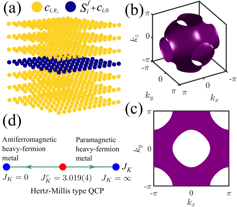
Figure 1: (a) Sketch of Kondo heterostructure, consisting of a two-dimensional array of magnetic impurities (blue dots) and three-dimensional itinerant conduction electrons, modeled by a tight-binding Hamiltonian on a cubic lattice (yellow dots). (b) Three-dimensional Fermi surface of conduction electrons. (c) Projected Fermi surface. (d) Ground-state phase diagram of model in Eq. (1), as extracted from QMC results.

II.1 Weak-coupling limit

At $J_{\mathrm{K}}=0$, spins and conduction electrons decouple. To set the stage, we will first discuss these degrees of freedom separately, and then investigate how they couple perturbatively in $J_{\mathrm{K}}$.

The spin and charge excitations of the conduction electrons are characterized by the noninteracting susceptibility

$$\chi^{0}(\boldsymbol{r}-\boldsymbol{r}^{\prime},\tau-\tau^{\prime})\equiv\frac{1}{4}\langle\hat{\boldsymbol{c}}^{\dagger}_{\boldsymbol{r}}(\tau)\boldsymbol{\sigma}\hat{\boldsymbol{c}}^{\phantom{\dagger}}_{\boldsymbol{r}}(\tau)\cdot\hat{\boldsymbol{c}}^{\dagger}_{\boldsymbol{r}^{\prime}}(\tau^{\prime})\boldsymbol{\sigma}\hat{\boldsymbol{c}}^{\phantom{\dagger}}_{\boldsymbol{r}^{\prime}}(\tau^{\prime})\rangle_{0}$$ (8)

with $\hat{\boldsymbol{c}}_{\boldsymbol{r}}=(c_{\boldsymbol{r},\uparrow},c_{\boldsymbol{r},\downarrow})$, and where the expectation value is taken with respect to $\hat{H}_{\text{Fermi}}$. To simplify the notation, we set $\boldsymbol{r}=(\boldsymbol{i},R_{z})$. The particle-hole symmetric conduction band remains invariant under the transformation $\hat{c}^{\dagger}_{\boldsymbol{r}}\rightarrow e^{i\boldsymbol{Q}\cdot\boldsymbol{r}}\hat{c}^{\phantom{\dagger}}_{\boldsymbol{r}}$ with $\boldsymbol{Q}=\left(\pi,\pi,\pi\right)$, such that

$$\chi^{0}(\boldsymbol{r},\tau)=\frac{3}{2}e^{i\boldsymbol{Q}\cdot\boldsymbol{r}}\left[\frac{1}{\left(2\pi\right)^{3}}\int_{\text{BZ}}d^{3}\boldsymbol{k}\,e^{i\boldsymbol{k}\cdot\boldsymbol{r}}e^{\tau\epsilon(\boldsymbol{k})}f(\epsilon(\boldsymbol{k}))\right]^{2},$$ (9)

where $\epsilon(\boldsymbol{k})=-2t(\cos k_{x}+\cos k_{y}+\cos k_{z})$, $f(\epsilon)$ is the Fermi function, and we have set the lattice constant to unity. From the above, one will see that at zero temperature,

$$\chi^{0}(\boldsymbol{0},\tau)=\frac{3}{2}\left(\int_{-\infty}^{0}d\epsilon\,e^{\tau\epsilon}N(\epsilon)\right)^{2}$$ (10)

where $N(\epsilon)=\frac{1}{\left(2\pi\right)^{3}}\int_{\text{BZ}}d^{3}\boldsymbol{k}\,\delta\left(\epsilon-\epsilon(\boldsymbol{k})\right)$ is the density of states. Since in three dimensions $N(\epsilon)$ has no singularity at the Fermi energy, $\epsilon_{\mathrm{F}}=0$, and since the long-imaginary-time behavior of the integral stems from energies close to the Fermi surface, we obtain the asymptotic form $\chi^{0}(\boldsymbol{0},\tau)\sim 1/\tau^{2}$ for large $\tau$. We now consider the spatial decay at equal time. For a spherical Fermi surface, the $\boldsymbol{k}$ integration can be computed exactly to obtain the large-distance behavior $\chi^{0}(\boldsymbol{r},0)\sim 1/|\boldsymbol{r}|^{4}$.

For the Heisenberg model, we follow Haldane’s derivation of the O(3) non-linear sigma model [16]. The starting point is a spin-coherent-state formulation of the path integral. In the large-$S$ limit and assuming dominant antiferromagnetic spin-spin fluctuations, the action for the local moments reads

$$S_{\text{AFM}}=\rho_{s}\int d^{2}\boldsymbol{x}d\tau\,\sum_{\mu}\left(\partial_{\mu}\boldsymbol{\Omega}(\boldsymbol{x},\tau)\right)^{2}.$$ (11)

In the above, we have neglected the Berry phase since it plays no dominant role in the ordered state, $\boldsymbol{\Omega}(\boldsymbol{x},\tau)$ is a space-time-dependent unit vector accounting for the dynamics of the antiferromagnetic O(3) order parameter, and $\mu$ runs over the temporal and spatial directions. Finally, we have set the spin wave velocity to unity. In the ordered state, the O(3) symmetry is reduced to O(2), and for spontaneous symmetry breaking along the $z$ direction we consider the ansatz

$$\boldsymbol{\Omega}(\boldsymbol{x},\tau)=\left(\boldsymbol{n}(\boldsymbol{x},\tau),\sqrt{1-\boldsymbol{n}^{2}(\boldsymbol{x},\tau)}\right)$$ (12)

where $\boldsymbol{n}=(n_{x},n_{y})$ denotes the transverse components of the order parameter, with $|\boldsymbol{n}|\ll 1$. Expanding in $|\boldsymbol{n}|$ gives, $S_{\text{AFM}}=S^{(0)}_{\text{AFM}}+S^{(1)}_{\text{AFM}}+\cdots$ with $S^{(0)}_{\text{AFM}}=\rho_{s}\int d^{2}\boldsymbol{x}d\tau\,\sum_{\mu}\left(\partial_{\mu}\boldsymbol{n}(\boldsymbol{x},\tau)\right)^{2}$ and $S^{(1)}_{\text{AFM}}=\frac{\rho_{s}}{4}\int d^{2}\boldsymbol{x}d\tau\,\sum_{\mu}\left(\partial_{\mu}\boldsymbol{n}^{2}(\boldsymbol{x},\tau)\right)^{2}$. Under the scale transformation $\boldsymbol{x}\rightarrow\lambda\boldsymbol{x}$, $\tau\rightarrow\lambda\tau$ and $\boldsymbol{n}\rightarrow\frac{\boldsymbol{n}}{\sqrt{\lambda}}$, $S^{(0)}_{\text{AFM}}$ remains invariant and accounts for the Lorentz-symmetric gapless transverse spin-spin fluctuations. Under this transformation, the magnon-magnon interactions described by $S^{(1)}_{\text{AFM}}$ scale as $1/\lambda$ and are hence irrelevant at the spin-wave fixed point. Higher orders in the expansion are even more irrelevant.

With this background, we can now couple the two systems perturbatively. Using fermion-coherent states for the conduction electrons and the spin-coherent states for the local moments, the partition function maps onto a bilinear fermionic problem interacting with the space-and-time-dependent spin-coherent state. At this point, one can integrate out the fermions and expand the resulting action up to second order in the Kondo coupling $J_{\mathrm{K}}$. Omitting the Berry phase, the resulting action reads

$$S=S_{\text{AFM}}+\Gamma\int d^{2}\boldsymbol{x}d^{2}\boldsymbol{x}^{\prime}d\tau d\tau^{\prime}\\ \boldsymbol{\Omega}(\boldsymbol{x},\tau)\chi^{0}_{\text{AFM}}(\boldsymbol{x}-\boldsymbol{x}^{\prime},\tau-\tau^{\prime})\boldsymbol{\Omega}(\boldsymbol{x}^{\prime},\tau^{\prime}).$$ (13)

Here, $\chi^{0}_{\text{AFM}}(\boldsymbol{x},\tau)$ $=\frac{3}{2}\left[\frac{1}{\left(2\pi\right)^{3}}\int_{\text{BZ}}d^{3}\boldsymbol{k}\,e^{i\boldsymbol{k}_{2}\cdot\boldsymbol{x}}e^{\tau\epsilon(\boldsymbol{k})}f(\epsilon(\boldsymbol{k}))\right]^{2}$ and $\Gamma\propto J_{\mathrm{K}}^{2}$. Note that the magnetic layer lies at $R_{z}=0$ and $\boldsymbol{k}=(\boldsymbol{k}_{2},k_{z})$.

Let us concentrate on the equal time spacial and local temporal correlations. In this case,

$$S \simeq S_{\text{AFM}}+\Gamma\int d^{2}\boldsymbol{x}d\tau d\tau^{\prime}\frac{\boldsymbol{\Omega}(\boldsymbol{x},\tau)\cdot\boldsymbol{\Omega}(\boldsymbol{x},\tau^{\prime})}{(\tau-\tau^{\prime})^{2}}$$

$$\quad+\Gamma\int d^{2}\boldsymbol{x}d^{2}\boldsymbol{x}^{\prime}d\tau\frac{\boldsymbol{\Omega}(\boldsymbol{x},\tau)\cdot\boldsymbol{\Omega}(\boldsymbol{x}^{\prime},\tau)}{|\boldsymbol{x}-\boldsymbol{x}^{\prime}|^{4}}.$$ (14)

The ansatz of Eq. (12) then gives $S=S^{(0)}+S^{(1)}+\cdots$ with

$$S^{(0)} =\rho_{s}\int d^{2}\boldsymbol{x}d\tau\left[\left(\partial_{x}\boldsymbol{n}(\boldsymbol{x},\tau)\right)^{2}+\left(\partial_{y}\boldsymbol{n}(\boldsymbol{x},\tau)\right)^{2}\right]$$

$$\quad+\Gamma\int d^{2}\boldsymbol{x}d\tau d\tau^{\prime}\frac{\boldsymbol{n}(\boldsymbol{x},\tau)\cdot\boldsymbol{n}(\boldsymbol{x},\tau^{\prime})}{(\tau-\tau^{\prime})^{2}}$$

$$\quad+\Gamma\int d^{2}\boldsymbol{x}d^{2}\boldsymbol{x}^{\prime}d\tau\frac{\boldsymbol{n}(\boldsymbol{x},\tau)\cdot\boldsymbol{n}(\boldsymbol{x}^{\prime},\tau)}{|\boldsymbol{x}-\boldsymbol{x}^{\prime}|^{4}}$$ (15)

and

$$S^{(1)} =\rho_{s}\int d^{2}\boldsymbol{x}d\tau\left[\left(\partial_{\tau}\boldsymbol{n}(\boldsymbol{x},\tau)\right)^{2}+\frac{1}{4}\sum_{\mu}\left(\partial_{\mu}\boldsymbol{n}^{2}(\boldsymbol{x},\tau)\right)^{2}\right]$$

$$\quad+\frac{\Gamma}{4}\int d^{2}\boldsymbol{x}d\tau d\tau^{\prime}\,\frac{\boldsymbol{n}^{2}(\boldsymbol{x},\tau)\boldsymbol{n}^{2}(\boldsymbol{x},\tau^{\prime})}{(\tau-\tau^{\prime})^{2}}$$

$$\quad+\frac{\Gamma}{4}\int d^{2}\boldsymbol{x}d^{2}\boldsymbol{x}^{\prime}d\tau\,\frac{\boldsymbol{n}^{2}(\boldsymbol{x},\tau)\boldsymbol{n}^{2}(\boldsymbol{x}^{\prime},\tau)}{|\boldsymbol{x}-\boldsymbol{x^{\prime}}|^{4}}.$$ (16)

Under the scale transformation $\boldsymbol{x}\rightarrow\lambda\boldsymbol{x}$, $\tau\rightarrow\lambda^{2}\tau$ and $\boldsymbol{n}\rightarrow\frac{\boldsymbol{n}}{\lambda}$, $S^{(0)}$ remains scale invariant and describes a Landau-damped Goldstone-mode fixed point with dynamical exponent $z=2$. At this fixed point, $S^{(1)}$ is irrelevant.

To conclude, the dynamical spin-structure factor in the weak-coupling limit is expected to show long-range magnetic order and to be described by Landau-damped Goldstone modes governed by the fixed-point action of Eq. (II.1). A corresponding spin-wave analysis, presented in Appendix D, confirms this point of view.

II.2 Mean-field approximation

In this section, we consider a mean-field approximation that accounts for Kondo screening as well as for magnetic ordering [17]. We use the pseudo-fermion representation $\boldsymbol{\hat{f}}_{\boldsymbol{i},\sigma}^{\dagger}=\left(\hat{f}^{\dagger}_{\boldsymbol{i},\uparrow},\hat{f}^{\dagger}_{\boldsymbol{i},\downarrow}\right)$ of the spin-1/2, $\hat{\boldsymbol{S}}_{\boldsymbol{i}}^{f}=\frac{1}{2}\boldsymbol{\hat{f}}^{\dagger}_{\boldsymbol{i}}\boldsymbol{\sigma}\boldsymbol{\hat{f}}^{\dagger}_{\boldsymbol{i}}$, that holds provided that we impose the constraint $\hat{Q}_{\boldsymbol{i}}=\boldsymbol{\hat{f}}^{\dagger}_{\boldsymbol{i}}\boldsymbol{\hat{f}}^{\phantom{\dagger}}_{\boldsymbol{i}}=1$. With this choice, the Kondo coupling can be written as

$$\boldsymbol{\hat{S}}_{\boldsymbol{i},R_{z}=0}^{c}\cdot\boldsymbol{\hat{S}}_{\boldsymbol{i}}^{f} =\hat{S}_{\boldsymbol{i},R_{z}=0}^{c,z}\hat{S}_{\boldsymbol{i}}^{f,z}$$

$$\quad-\frac{1}{4}\sum_{\sigma}\left(\hat{c}_{\boldsymbol{i},R_{z}=0,\sigma}^{\dagger}\hat{f}^{\phantom{\dagger}}_{\boldsymbol{i},\sigma}+\hat{f}_{\boldsymbol{i},-\sigma}^{\dagger}\hat{c}_{\boldsymbol{i},R_{z}=0,-\sigma}^{\phantom{\dagger}}\right)^{2},$$ (17)

where $\hat{S}_{\boldsymbol{i},R_{z}=0}^{c,z}=\frac{1}{2}\hat{\boldsymbol{c}}_{\boldsymbol{i},R_{z}=0}^{\dagger}\sigma_{z}\hat{\boldsymbol{c}}_{\boldsymbol{i},R_{z}=0}^{\phantom{\dagger}}$.

The above reformulation allows us to carry out mean-field approximations that account for the Kondo effect, as described in the large-$N$ limit, and magnetism. We note that this mean-field decomposition can be formulated for an SU($N$)-symmetric Kondo lattice model [18], in which magnetism driven by the RKKY interaction becomes a $1/N$ effect. In the mean-field approximation, squared order-parameter fluctuations are neglected, i.e.,

$$\hat{O}^{2} =\left(\left\langle\hat{O}\right\rangle+\Delta\hat{O}\right)^{2}=\left\langle\hat{O}\right\rangle^{2}+2\left\langle\hat{O}\right\rangle\Delta\hat{O}+\left(\Delta\hat{O}\right)^{2}$$

$$\approx 2\left\langle\hat{O}\right\rangle\hat{O}-\left\langle\hat{O}\right\rangle^{2},$$ (18)

where $\Delta\hat{O}=\hat{O}-\left\langle\hat{O}\right\rangle$ are the fluctuations. Here, we consider the following order parameters

$$\begin{cases}\left\langle\hat{S}_{\boldsymbol{i},R_{z}=0}^{c,z}\right\rangle=-m_{c}e^{i\boldsymbol{Q}\cdot\boldsymbol{i}},\\ \left\langle\hat{S}_{\boldsymbol{i}}^{f,z}\right\rangle=m_{f}e^{i\boldsymbol{Q}\cdot\boldsymbol{i}},\\ \left\langle\hat{c}_{\boldsymbol{i},R_{z}=0,\sigma}^{\dagger}\hat{f}_{\boldsymbol{i},\sigma}^{\phantom{\dagger}}+\hat{f}_{\boldsymbol{i},-\sigma}^{\dagger}\hat{c}_{\boldsymbol{i},R_{z}=0,-\sigma}^{\phantom{\dagger}}\right\rangle=V,\end{cases}$$ (19)

where $V$ accounts for the hybridization between the $c$ and $f$ fermions, $m_{c}$ and $m_{f}$ denotes the magnetizations arising from conduction electrons and impurity spins, respectively and $\boldsymbol{Q}=(\pi,\pi)$. By combining Eqs. (17)-(19), we obtain the effective mean-field Hamiltonian

$$\hat{H}_{\text{MF}} =\hat{H}_{\mathrm{Fermi}}+\sum_{\boldsymbol{i}}\lambda_{\boldsymbol{i}}\left(\hat{f}_{\boldsymbol{i},\sigma}^{\dagger}\hat{f}_{\boldsymbol{i},\sigma}^{\phantom{\dagger}}-1\right)$$

$$\quad-\frac{J_{\mathrm{K}}V}{2}\sum_{\boldsymbol{i},\sigma}\left(\hat{c}_{\boldsymbol{i},R_{z}=0,\sigma}^{\dagger}\hat{f}_{\boldsymbol{i},\sigma}^{\phantom{\dagger}}+\text{h.c.}\right)$$

$$\quad+J_{\mathrm{K}}\sum_{\boldsymbol{i}}e^{i\boldsymbol{Q}\cdot\boldsymbol{i}}\left(m_{f}\hat{S}_{\boldsymbol{i},R_{z}=0}^{c,z}-m_{c}\hat{S}_{\boldsymbol{i}}^{f,z}\right)$$

$$\quad-J_{\mathrm{H}}m_{f}z_{c}\sum_{\boldsymbol{i}}e^{i\boldsymbol{Q}\cdot\boldsymbol{i}}\hat{S}_{\boldsymbol{i}}^{f,z}+\epsilon_{0}$$ (20)

where $\epsilon_{0}=L^{2}\left[2J_{\mathrm{H}}\left(m_{f}\right)^{2}+J_{\mathrm{K}}m_{c}m_{f}+J_{\mathrm{K}}V^{2}/2\right]$ and $z_{\mathrm{c}}=4$ corresponds to the coordination number of the square lattice. To suppress the charge fluctuations in the pseudo fermion sector, we introduce the Lagrange parameter ${\lambda_{\boldsymbol{i}}}$ in the first line of Eq. (20), which imposes the constraint $\hat{Q}_{\boldsymbol{i}}=1$ at each site.

In the above, we have not accounted for a spinon description of the quantum antiferromagnet, in which the pseudo fermions delocalize in the magnetic impurity plane. In the magnetic phase, where the hybridization matrix element vanishes, we can justify this choice from our knowledge that the two-dimensional Heisenberg model on the square lattice does not have a fractionalized ground state. In the heavy-fermion state, $V\neq 0$, the $f$ pseudo fermions acquire electric charge and lose their gauge charge via the Higgs mechanism, such that they can acquire a dispersion relation [8, 9]. The mean-field Hamiltonian $\hat{H}_{\text{MF}}$ is bilinear in the fermions and can hence be solved numerically exactly in polynomial time for a given set of order parameters. For an analytical calculation in the heavy-fermion state, we refer to Appendix E. The order parameters are obtained by the minimizing the free energy $\partial F_{\text{MF}}/\partial m_{c}=\partial F_{\text{MF}}/\partial m_{f}=\partial F_{\text{MF}}/\partial V=0$, leading to a set of self-consistent equations

$$\begin{cases}m_{c}=-\frac{1}{2L^{2}}\sum_{\boldsymbol{k}_{2},\sigma}\left(-1\right)^{\sigma}\left\langle\hat{c}_{\boldsymbol{k}_{2}+\boldsymbol{Q},R_{z}=0,\sigma}^{\dagger}\hat{c}_{\boldsymbol{k}_{2},R_{z}=0,\sigma}^{\phantom{\dagger}}\right\rangle,\\ m_{f}=\frac{1}{2L^{2}}\sum_{\boldsymbol{k}_{2},\sigma}\left(\left(-1\right)^{\sigma}\left\langle\hat{f}_{\boldsymbol{k}_{2}+\boldsymbol{Q},\sigma}^{\dagger}\hat{f}_{\boldsymbol{k}_{2},\sigma}^{\phantom{\dagger}}\right\rangle\right),\\ V=\frac{1}{2L^{2}}\sum_{\boldsymbol{k}_{2},\sigma}\left(\left\langle\hat{c}_{\boldsymbol{k}_{2},R_{z}=0,\sigma}^{\dagger}\hat{f}_{\boldsymbol{k}_{2},\sigma}^{\phantom{\dagger}}+\hat{f}_{\boldsymbol{k}_{2},\sigma}^{\dagger}\hat{c}_{\boldsymbol{k}_{2},R_{z}=0,\sigma}^{\phantom{\dagger}}\right\rangle\right),\\ \frac{1}{L^{2}}\sum_{\boldsymbol{i},\sigma}\left\langle\hat{f}_{\boldsymbol{i},\sigma}^{\dagger}\hat{f}_{\boldsymbol{i},\sigma}^{\phantom{\dagger}}\right\rangle=1.\end{cases}$$ (21)

The last equation in Eq. (21) corresponds to the half-filling constraint for the pseudo fermions. At $\lambda=0$, the mean-field Hamiltonian of Eq. (20) is particle-hole symmetric such that this choice of the Lagrange parameter satisfies the constraint on average. Technical details concerning the numerical solution of the self-consistency equations are provided in Appendix A.

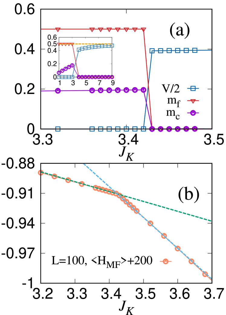
Figure 2: (a) Mean-field order parameters at zero temperature. Here, $t=1$, $J_{\mathrm{H}}=0.5$, and we set $L=100$. The inset shows the order parameters over a larger range, confirming the analytical result $V=1$ in the strong-coupling limit [Eq. (LABEL:MF_strong_coupling.eq)]. (b) Free energy as function of $J_{\mathrm{K}}$. Both (a) and (b) support a first-order transition.

The resulting mean-field phase diagram at zero temperature is presented in Fig. 2(a). Here, we have set the hopping parameter for the conduction electrons to $t=1$, thereby setting the unit of energy, fixed the Heisenberg coupling to $J_{\mathrm{H}}/t=0.5$, and varied the Kondo coupling $J_{\mathrm{K}}$. The phase diagram is divided into two regimes. At weak Kondo coupling, $J_{\mathrm{K}}\ll 1$, we observe an antiferromagnetic metallic phase, in which the mean-field parameters satisfy $m_{c}\neq 0$, $m_{f}\neq 0$, and $V=0$. At strong Kondo coupling, $J_{\mathrm{K}}\gg 1$, the model is in a paramagnetic heavy-fermion phase, characterized by $m_{c}=m_{f}=0$ and $V\neq 0$. These two phases are separated by a direct first-order transition around $J_{\mathrm{K}}\approx 3.42$, where the order parameters show discontinuities. A cusp in the ground state, Fig. 2(b) reflects the corresponding level crossing, consistent with the first-order nature of the transition.

We expect that the single-particle spectral function $A_{c/f}(\boldsymbol{k}_{2},\omega)=-\frac{1}{\pi}\text{Im}G^{\text{ret}}_{c/f}(\boldsymbol{k}_{2},\omega)$ will have distinct features in each phase. Here, $G_{d}^{\text{ret}}(\boldsymbol{k}_{2},\omega)=-i\int_{0}^{\infty}dt\,e^{i\omega t}\sum_{\sigma}\left<\big{\{}\hat{d}_{\boldsymbol{k}_{2},\sigma}(t),\hat{d}_{\boldsymbol{k}_{2},\sigma}^{\dagger}(0)\big{\}}\right>$, with $\hat{d}_{\boldsymbol{k}_{2},\sigma}=\hat{c}_{\boldsymbol{k}_{2},R_{z}=0,\sigma}$ for the conduction-electron spectral function, and $\hat{d}_{\boldsymbol{k}_{2},\sigma}=\hat{f}_{\boldsymbol{k}_{2},\sigma}$ for the pseudo-fermion spectral function. In Fig. 3, we plot the local density of states, $A_{c/f}(\omega)=\frac{1}{L^{2}}\sum_{\boldsymbol{k}_{2}}A_{c/f}(\boldsymbol{k}_{2},\omega)$ in the aforementioned two phases, using $J_{\mathrm{K}}=2.00$ and $J_{\mathrm{K}}=5.00$. Furthermore, we are interested in states characterized by all order parameters being non-zero. Although such state are not realized as ground states at the level of the mean-field approximation, it reflects the coexistence of magnetic order and Kondo screening, as observed in the forthcoming quantum Monte Carlo results.

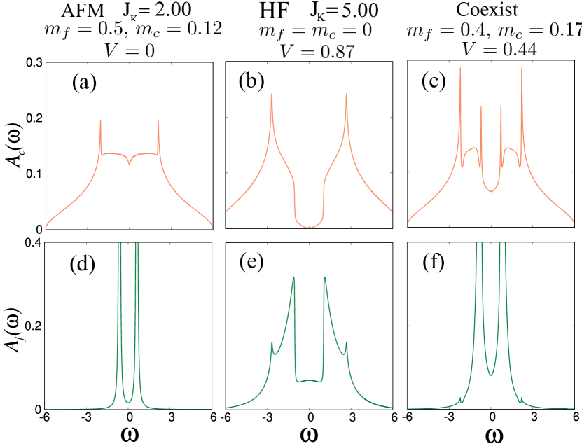
Figure 3: Local density of states $A_{c}(\omega)$ (top) and $A_{f}(\omega)$ (bottom) in antiferromagnetic (first column), heavy-fermion (second column) and coexistence (third column) states in mean-field approximation. The corresponding mean-field parameters are given in the title of each column.

For $m_{c}\neq 0$, $m_{f}\neq 0$, and $V=0$, as observed at $J_{\mathrm{K}}=2.00$, the $f$ fermions are localized. $A_{f}(\omega)$, shown in Fig. 3(d), consists of two Dirac $\delta$ functions and the origin of the gap stems from the Weiss mean field $m_{f}\neq 0$. This is confirmed by the momentum-resolved $f$ spectral function, shown in Fig. 4(d), which exhibits two flat bands. For the above mean-field parameters, the conduction-electron resolvant matrix reads $G_{c,\sigma}(z)=\left(G_{c,\sigma,0}^{-1}(z)-\Sigma_{c,\sigma}\right)^{-1}$ with $\left[G_{c,\sigma,0}^{-1}(z)\right]_{\boldsymbol{k},\boldsymbol{k}^{\prime}}=\delta_{\boldsymbol{k},\boldsymbol{k}^{\prime}}(z-\epsilon(\boldsymbol{k}))$, $\left[\Sigma_{c,\sigma}\right]_{\boldsymbol{k},\boldsymbol{k}^{\prime}}=\frac{\sigma J_{\mathrm{K}}m_{f}}{2L}\delta_{\boldsymbol{k}_{2},\boldsymbol{k}^{\prime}_{2}+\boldsymbol{Q}}$, and $z$ a complex frequency. Here, $\boldsymbol{k}=\left(\boldsymbol{k}_{2},k_{z}\right)$ and $\boldsymbol{Q}=(\pi,\pi)$. From this form, one can derive the spectral function, plotted in Fig. 4(a),

$$A_{c}(\boldsymbol{k}_{2},\omega)=-\frac{1}{\pi}\text{Im}\frac{1}{g_{0}^{-1}(\boldsymbol{k}_{2},\omega)-\frac{(J_{\mathrm{K}}m_{f})^{2}}{4}\,g_{0}(\boldsymbol{k}_{2}+\boldsymbol{Q},\omega)}$$ (22)

with $g_{0}(\boldsymbol{k}_{2},\omega)=\frac{1}{L}\sum_{k_{z}}\frac{1}{\omega+i0^{+}-\epsilon(\boldsymbol{k}_{2},k_{z})}$. In the absence of magnetic ordering, the spectral function describes a continuum of extended Bloch states in all three directions. At finite values of $m_{c}$, we observe a back folding of this structure due to scattering off the magnetic Bragg peak. In the vicinity of the $\boldsymbol{M}$ point and $\omega\simeq\pm 2.1t$, we observe a pole that is detached from the continuum. Note that at the $\boldsymbol{M}$ point, the continuum of states obtained from $g_{0}(\boldsymbol{k}_{2},\omega)$ is bounded by $\omega=\pm 2$. Let $|\boldsymbol{k}_{2},k_{z}\rangle$ be the wave function corresponding to the pole. Since the two-dimensional $\boldsymbol{k}_{2}$ vector is a conserved quantity, up to a reciprocal lattice vector of the magnetic Brillouin zone, an electron in this state cannot decay into an extended three-dimensional state. Hence, we expect the wave function to have a two-dimensional character. That is, $|\boldsymbol{k}_{2},R_{z}\rangle\equiv\frac{1}{\sqrt{L}}\sum_{k_{z}}e^{-ik_{z}R_{z}}|\boldsymbol{k}_{2},k_{z}\rangle$ should decay exponentially as a function of $R_{z}$, with $R_{z}=0$ denoting the magnetic layer. In Appendix E, we provide an explicit calculation in the paramagnetic phase, demonstrating this point. The two dimensionality of the pole shows up in Fig. 3(a). Here, we see the saddle point of the dispersion at the $\boldsymbol{M}$ wave vector leads to a two-dimensional van-Hove singularity with characteristic logarithmic divergence.

–

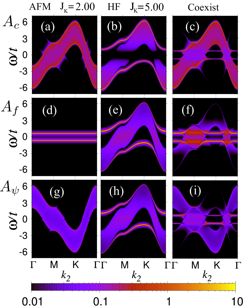
Figure 4: Fermion spectral functions $A_{c}(\boldsymbol{k}_{2},\omega)$ (top row), $A_{f}(\boldsymbol{k}_{2},\omega)$ (center row), and $A_{\psi}(\boldsymbol{k}_{2},\omega)$ (bottom row) in antiferromagnetic (left column), heavy-fermion (center column) and coexistence (right column) phases in mean-field approximation. Here, we consider the path $\boldsymbol{\Gamma}(0,0)\rightarrow\boldsymbol{M}(\pi,0)\rightarrow\boldsymbol{K}(\pi,\pi)\rightarrow\boldsymbol{\Gamma}(0,0)$.

At large $J_{\mathrm{K}}=5.00$, shown in Figs. 3(b,e) and 4(b,e), only $V$ takes a nonvanishing value. Here the $f$ electron delocalizes and participates in the Luttinger volume. This notion can be made precise, since we can view the heterostructure as a two-dimensional Bravais lattice with a unit cell consisting of $L$ conduction electrons and one pseudo-fermion. In the paramagnetic heavy-fermion phase, the pseudo-fermion spectral function is given by

$$A_{f}(\boldsymbol{k}_{2},\omega)=-\frac{1}{\pi}\text{Im}\frac{1}{\omega+i0^{+}-\left(J_{\mathrm{K}}V/2\right)^{2}g_{0}(\boldsymbol{k}_{2},\omega)}.$$ (23)

For values of $\boldsymbol{k}_{2}$ with $\cos k_{x}+\cos k_{y}=0$, defining the Fermi surface of the two-dimensional tight-binding model on the square lattice, the above form matches the mean-field result of a single impurity in a one-dimensional metallic host. Here, we observe a resonance at the Fermi energy for the $f$ spectral function, and a dip in the $c$ spectral function. These features are apparent in Figs. 3(b,e) and 4(b,e). The momentum-resolved $f$ spectral function, 4(e), shows well-defined poles. Following the same discussion as above, and as explicitly computed in Appendix E, these poles correspond to two-dimensional states. In the vicinity of the $\boldsymbol{M}$ and $\boldsymbol{\Gamma}$ points in the two-dimensional Brillouin zone, they form a narrow band that leads to an enhanced density of states, very visible in Fig. 3(b,e).

Finally, for a coexistence state, all mean-field order parameters take nonvanishing values. For our analysis, we choose the mean-field parameters $m_{c}=0.17$, $m_{f}=0.40$, and $V=0.438$. The dominant features in such state, as shown in Figs. 3(c,f) and 4(c,f), can be understood by starting from the paramagnetic heavy-fermion phase and allowing for $\boldsymbol{Q}=(\pi,\pi)$ scattering, which leads to shadow bands in the extended zone scheme.

In an exact numerical calculation, we do not have access to the pseudo fermion, and it is convenient to consider a so-called composite fermion operator defined as $\hat{\psi}_{\boldsymbol{i},\sigma}^{\dagger}=\sum_{\sigma^{\prime}}\hat{c}_{\boldsymbol{i},R_{z}=0,\sigma^{\prime}}^{\dagger}\boldsymbol{\sigma}_{\sigma^{\prime},\sigma}\cdot\hat{\boldsymbol{\mathit{S}}}^{f}_{\boldsymbol{i}}$ [19, 20, 21, 22, 8, 9]. By means of a canonical Shrieffer-Wolff transformation [23], one can derive the Kondo lattice model from an Anderson model in the limit where charge fluctuations on the localized impurity orbitals is suppressed. In this framework, the composite fermion operator merely corresponds to the Schrieffer-Wolff transformation of the fermion creation operator on localized impurity orbitals [22]. In addition, one can represent the Kondo coupling as the hybridization of the composite fermion and $c$ fermion, $\frac{1}{2}\sum_{\sigma}(\hat{\psi}_{\boldsymbol{i},\sigma}^{\dagger}\hat{c}_{\boldsymbol{i},R_{z}=0,\sigma}+\hat{c}_{\boldsymbol{i},R_{z}=0,\sigma}^{\dagger}\hat{\psi}_{\boldsymbol{i},\sigma})=\hat{\boldsymbol{S}}_{\boldsymbol{i},R_{z}=0}^{c}\cdot\hat{\boldsymbol{S}}_{\boldsymbol{i}}^{f}$. In the mean-field approximation, the Green’s function of the composite fermion can be computed by expressing it as a convolution of single-particle Green’s functions via Wick’s theorem. The resulting momentum-dependent spectral function $A_{\psi}(\boldsymbol{k}_{2},\omega)$ is depicted for the three representative values of $J_{\mathrm{K}}$ in Figs. 4(g)-(i).

We first focus on the behavior of the composite fermion in a Kondo-screened phase. In the large-$N$ limit, the composite fermion reads $\hat{\psi}^{\dagger}_{\boldsymbol{i},\sigma}\propto\left\langle\hat{D}_{\boldsymbol{i}}\right\rangle\frac{2}{N}f^{\dagger}_{\boldsymbol{i},\sigma}$[8], where $N$ is the number of fermion components, $\sigma=1,\dots,N$, and $\hat{D}_{\boldsymbol{i}}=\sum_{\sigma=1}^{N}\hat{f}_{\boldsymbol{i},\sigma}^{\phantom{\dagger}}\hat{c}_{\boldsymbol{i},R_{z}=0,\sigma}^{\dagger}$ the hybridization. The Kondo-screened phase is characterized by a finite hybridization parameter $V$, and we expect the spectral function of $\psi$ fermion to follow that of the $f$ fermion. By comparing the results presented in Figs. 4(e) and (h), we see that the mean-field calculation agrees with the large-$N$ approximation in the Kondo-screened phase.

In the antiferromagnetic metal phase, the mean-field hybridization parameter $V$ vanishes, so that the $f$ electron is no longer related to the composite fermion $\psi$. The behavior of the composite fermion spectral function in Fig. 4(g) can be understood within a large-$S$ approximation [8]. Using the Holstein-Primakoff representation of the spin algebra and at lowest order in $1/S$, we obtain $\sum_{\sigma}G^{\psi}_{\boldsymbol{i},\boldsymbol{j}}(\tau)=S^{2}\sum_{\sigma}\left\langle\hat{c}_{\boldsymbol{i},\sigma}(0)\hat{c}_{\boldsymbol{j},\sigma}^{\dagger}(\tau)\right\rangle e^{i\boldsymbol{Q}\cdot(\boldsymbol{j}-\boldsymbol{i})}$. Hence, the composite fermion Green’s function can be obtained from that of the $c$ fermions, albeit with momentum shifted by the magnetic wave vector $\boldsymbol{Q}$. This statement is verified upon comparing Figs. 4(a) and 4(g).

III QMC simulations

We use the ALF [24, 25] implementation of the finite-temperature [26, 13, 27] and projective [28, 29] auxiliary-field QMC algorithms to perform large-scale simulations of the model defined in Eq. (1). For the QMC simulations, we consider the Hamiltonian,

$$\hat{H}_{\text{QMC}} =-t\sum_{\boldsymbol{k}_{2},\sigma,R_{z},R_{z}^{\prime}}\hat{c}_{\boldsymbol{k}_{2},R_{z},\sigma}^{\dagger}T(\boldsymbol{k}_{2})_{R_{z},R_{z}^{\prime}}^{\phantom{\dagger}}\hat{c}_{\boldsymbol{k}_{2},R_{z}^{\prime},\sigma}^{\phantom{\dagger}}\allowdisplaybreaks[1]$$

$$\quad-\frac{J_{\mathrm{K}}}{4}\sum_{\boldsymbol{i}}\left(\sum_{\sigma}\hat{c}_{\boldsymbol{i},R_{z}=0,\sigma}^{\dagger}\hat{f}_{\boldsymbol{i},\sigma}+\hat{f}_{\boldsymbol{i},\sigma}^{\dagger}\hat{c}_{\boldsymbol{i},R_{z}=0,\sigma}\right)^{2}\allowdisplaybreaks[1]$$

$$\quad-\frac{J_{\mathrm{H}}}{4}\sum_{\left\langle\boldsymbol{i},\boldsymbol{j}\right\rangle}\left(\sum_{\sigma}\hat{f}_{\boldsymbol{i},\sigma}^{\dagger}\hat{f}_{\boldsymbol{j},\sigma}+\hat{f}_{\boldsymbol{j},\sigma}^{\dagger}\hat{f}_{\boldsymbol{i},\sigma}\right)^{2}\allowdisplaybreaks[1]$$

$$\quad+\frac{U}{2}\sum_{\boldsymbol{i}}\left(\sum_{\sigma}\hat{f}_{\boldsymbol{i},\sigma}^{\dagger}\hat{f}_{\boldsymbol{i},\sigma}-1\right)^{2},$$ (24)

with $T(\boldsymbol{k}_{2})_{R_{z},R_{z}^{\prime}}=-2t(\cos k_{x}+\cos k_{y})\delta_{R_{z},R_{z}^{\prime}}-t\delta_{|R_{z}-R_{z}^{\prime}|,1}-t(\delta_{R_{z},L-1}\delta_{R^{\prime}_{z},0}+\delta_{R_{z},0}\delta_{R^{\prime}_{z},L-1})$ and $\hat{f}_{\boldsymbol{i},\sigma}$ the pseudo-fermion operator. The Hubbard-$U$ interaction in Eq. (24) suppresses charge fluctuations of the pseudo fermion. Crucially, the local $f$-fermion parity, $(-1)^{\hat{n}^{f}_{\boldsymbol{i}}}$, is a conserved quantity, such that the unphysical even-parity states are suppressed exponentially as $\beta U$ grows. In the odd-parity sector, $\hat{H}_{\text{QMC}}$ is equivalent to the KLM-hetero Hamiltonian, $\left.\hat{H}_{\text{QMC}}\right|_{\hat{n}_{\boldsymbol{i}}^{f}=1}=\hat{H}_{\text{KLM-hetero}}$. In the practical finite-temperature (projective) simulations, we keep the product $\beta U>10$ ($2\Theta U>10$, where $\Theta$ is the projection length), which is sufficient to suppress the charge fluctuations of the ${f}$ fermion.

Eq. (24) provides a U(1)-gauge-theory description of the Kondo-lattice problem. Following the path-integral formalism used in Ref. [9], we introduce bosonic fields $b_{\boldsymbol{i}}(\tau)\propto\boldsymbol{c}^{\dagger}_{\boldsymbol{i}}(\tau)\boldsymbol{f}_{\boldsymbol{i}}(\tau)$ and $b^{f}_{\boldsymbol{i},\boldsymbol{j}}(\tau)\propto\boldsymbol{f}^{\dagger}_{\boldsymbol{i}}(\tau)\boldsymbol{f}_{\boldsymbol{j}}(\tau)$ by decomposing the perfect square terms parametrized by $J_{\mathrm{K}}$ and $J_{\mathrm{H}}$ in Eq. (24), where $\boldsymbol{c}_{\boldsymbol{i}}(\tau)$ and $\boldsymbol{f}_{\boldsymbol{i}}(\tau)$ are the Grassmann fields of the $c$ and $f$ fermion operators. At $U=\infty$, the action has local U(1) gauge invariance. $\boldsymbol{f}_{\boldsymbol{i}}(\tau)$ and $b_{\boldsymbol{i}}(\tau)$ are the U(1)-gauge-charged field variables. One can define the gauge-neutral composite fermion field as $\boldsymbol{\tilde{f}}_{\boldsymbol{i}}(\tau)=e^{i\varphi_{\boldsymbol{i}}(\tau)}\boldsymbol{f}_{\boldsymbol{i}}(\tau)$ with $e^{i\varphi_{\boldsymbol{i}}(\tau)}=\frac{b_{\boldsymbol{i}}(\tau)}{\left|b_{\boldsymbol{i}}(\tau)\right|}$. The composite fermion field carries electron charge and spin $1/2$. More importantly, the field variable $\boldsymbol{\tilde{f}}_{\boldsymbol{i}}(\tau)$ corresponds to the Grassmann variable of the composite fermion operator $\boldsymbol{\tilde{f}}_{\boldsymbol{i}}\propto\boldsymbol{\psi}_{\boldsymbol{i}}=\boldsymbol{S}_{\boldsymbol{i}}\cdot\boldsymbol{\sigma}\boldsymbol{c}_{\boldsymbol{i}}$. This relation provides a route to understand the dynamic-spin-correlation behavior from the heavy-fermion band structure. We will come back to this point in the next section.

In the QMC simulations, we treat the finite-size Kondo heterostructure as a two-dimensional lattice containing $L\times L$ unit cells with $L+1$ orbitals per in-plane unit cell. The orbitals refer to the $z$-axis degrees of freedom. We use two techniques to reduce the finite-size effects in the lattice simulations. One is to follow the technique suggested in Ref. [30], by including an orbital magnetic field of strength $B=\phi_{0}/L^{2}$ in the $z$ direction. Another technique we use is to average over twisted boundary conditions in the $z$ direction [31]. To achieve this, we consider a distinct twist on every process during the parallel computations. Averaging over parallel runs then amounts to averaging over all possible twisted boundary conditions. The details of this technique are presented in Appendix B.

IV Results

In this section, we discuss our QMC results. We consider three-dimensional systems with linear lattice sizes $L=4,6,8,10,12$, and a mix of finite-temperature and zero-temperature projective methods. In our simulations, we set $t=1$ to define the unit energy, fix $J_{\mathrm{H}}/t=0.5$ and vary the Kondo coupling. For projective QMC simulations, we consider the projection length parameter $\Theta=40$ to ensure convergence of the results.

IV.1 Phase diagram

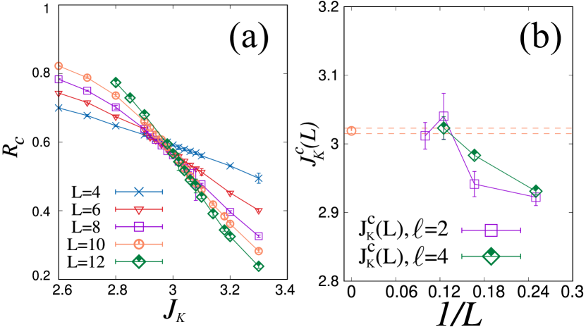
Figure 5: (a) Correlation ratio $R_{\mathrm{c}}(L,J_{\mathrm{K}})$ as function of Kondo coupling $J_{\mathrm{K}}$ from projective QMC for different lattice sizes $L$. (b) Finite-size critical point $J_{\mathrm{K}}^{\mathrm{c}}(L)$ as function $1/L$. The extrapolation towards the thermodynamic limit indicates a single quantum critical point at $J_{\mathrm{K}}^{\mathrm{c}}=3.019(4)$.

From the mean-field analysis, we anticipate at least one magnetic quantum phase transition as a function of $J_{\mathrm{K}}$. To pin down the location of a possible phase transition, we use a renormalization-group-(RG)-invariant quantity, the correlation ratio, given by

$$R_{\mathrm{c}}\left(\left(J_{\mathrm{K}}-J_{\mathrm{K}}^{\mathrm{c}}\right)L^{1/\nu},L^{z}/\beta,L^{-\omega}\right)=1-\frac{C_{f}(\boldsymbol{Q}+d\boldsymbol{k}_{2},0)}{C_{f}(\boldsymbol{Q},0)}$$ (25)

where $C_{f}(\boldsymbol{k}_{2},0)$ is the spin structure factor of the impurity spins,

$$C_{f}\left(\boldsymbol{k}_{2},\tau\right)=\sum_{\boldsymbol{k}_{2}}e^{-i\boldsymbol{k}_{2}\cdot(\boldsymbol{i}-\boldsymbol{j})}\left\langle\hat{S}_{\boldsymbol{i}}^{f}(\tau)\hat{S}_{\boldsymbol{j}}^{f}(0)\right\rangle,$$ (26)

and $d\boldsymbol{k}_{2}=\left(2\pi/L,0\right)$ is the smallest momentum difference on the finite-size system. The RG-invariant quantity $R_{\mathrm{c}}$ approaches one in the magnetically-ordered phase and drops to zero for short-ranged spin correlations. Since we a priori do not know the value of the dynamical exponent $z$, we have used the projective algorithm, such that we can set $L^{z}/\beta=0$ in the above equation. If the corrections to scaling are small (i.e., $\omega$ is large), we expect a universal crossing at $J_{\mathrm{K}}^{\mathrm{c}}$. In Fig. 5(a), we plot the result of $R_{\mathrm{c}}$ for $L=4,6,8,10,12$ at zero temperature. The finite-size critical points $J_{\mathrm{K}}^{\mathrm{c}}(L)$ is defined by the intersection of the correlation ratio between different system sizes, $R_{\mathrm{c}}(J_{\mathrm{K}}^{\mathrm{c}}(L),L)=R_{\mathrm{c}}(J_{\mathrm{K}}^{\mathrm{c}}(L),L+\ell)$. In Fig. 5(b), we consider $\ell=2,4$, and use a polynomial fit to determine the crossing point. We see that $J_{\mathrm{K}}^{\mathrm{c}}(L)$ drifts as a function of growing size and stabilizes to $J_{\mathrm{K}}^{\mathrm{c}}=3.019(4)$ at the two largest system sizes in our calculation. As we will demonstrate below, in contrast to the mean-field result, the QMC spectral functions indicate that hybridization between conduction electrons and local moments occurs throughout the magnetic phase. The QMC phase diagram therefore consists of just two different phases: An antiferromagnetic heavy-fermion phase for small $J_{\mathrm{K}}<J_{\mathrm{K}}^{\mathrm{c}}$ and a paramagnetic heavy-fermion phase for large $J_{\mathrm{K}}>J_{\mathrm{K}}^{\mathrm{c}}$, see Fig. 1(d).

IV.2 Spin spectral function

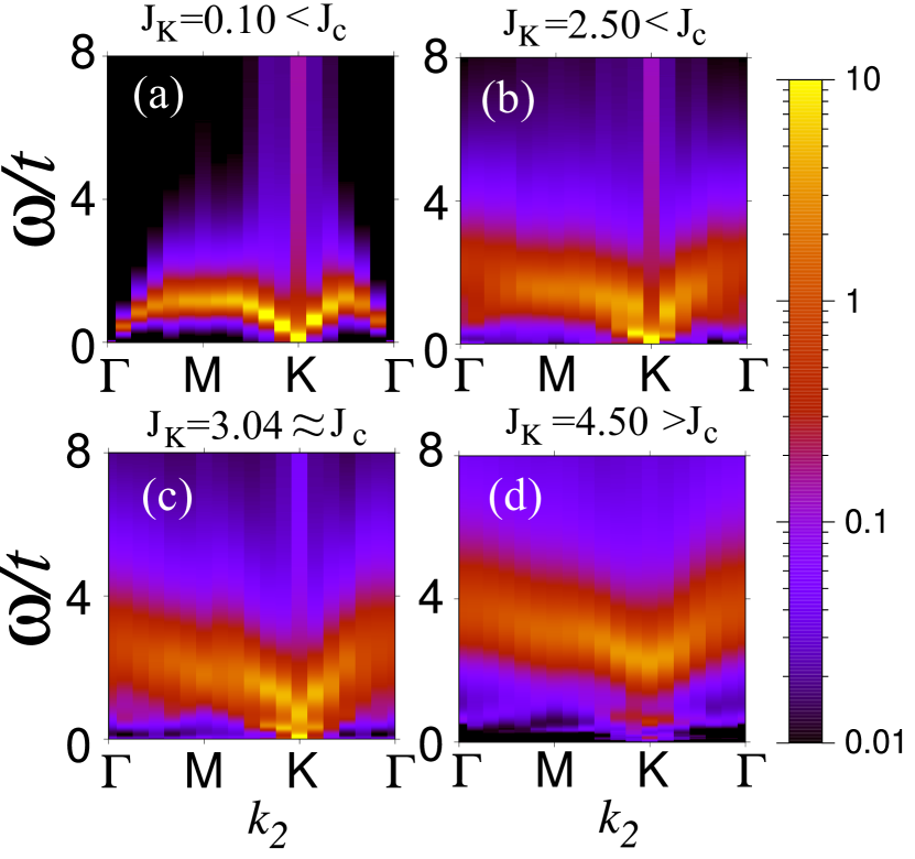
Figure 6: Spin spectral function $S(\boldsymbol{k}_{2},\omega)$ along a high-symmetry path in the Brillouin zone from finite-temperature QMC for different values of $J_{\mathrm{K}}$, using $\beta=40$ and $L=12$.

We turn our attention on the spin susceptibility of the magnetic impurity layer. Using the ALF [24] implementation of the stochastic Maximum Entropy method [32, 33], we extract the the dynamical spin structure factor $S(\boldsymbol{k}_{2},\omega)=\chi^{\prime\prime}_{f}(\boldsymbol{k}_{2},\omega)/[1-\exp(-\beta\omega)]$ from imaginary time spin correlation function. Specifically,

$$C_{f}\left(\boldsymbol{k}_{2},\tau\right)=\frac{1}{\pi}\int d\omega\,\frac{e^{-\tau\omega}}{1-e^{-\beta\omega}}\chi^{\prime\prime}_{f}(\boldsymbol{k}_{2},\omega).$$ (27)

At weak coupling, such as $J_{\mathrm{K}}=0.50$, Fig. 6(a), the dominant features of the dynamical spin structure factor follow the spin-wave result with a linear mode around the ordering wave vector $\boldsymbol{Q}=(\pi,\pi)$. Upon increasing the Kondo coupling to $J_{\mathrm{K}}=2.50$, Fig. 6(b), which is still in the magnetically-ordered phase, we observe marked differences from the spin-wave result: The spectral weight broadens and the data is consistent with a lower edge of the spectra that follows $\omega\propto(\boldsymbol{k}_{2}-\boldsymbol{Q})^{2}$ near $\boldsymbol{Q}$. This is consistent with the notion of Landau-damped Goldstone modes originating from the Kondo coupling of the spins to the metallic host, as presented in Sec. II.1 and discussed in Appendix D. Fig. 6(c) demonstrates that this feature is apparent up to the critical point $J_{\mathrm{K}}^{\mathrm{c}}$. At strong coupling, $J_{\mathrm{K}}=4.50>J_{\mathrm{K}}^{\mathrm{c}}$, Fig. 6(d), we are in the paramagnetic heavy-fermion phase. The absence of long-range magnetic order with associated Bragg peaks at the antiferromagnetic wave vector leads to a strong suppression of low-energy weight. We, however, still observe low-energy spectral weight: The heavy-fermion phases are characterized by the emergence of the composite fermion operator. As mentioned above, and within a field-theoretical framework, this can be understood in terms of a Higgs mechanism in which $e^{i\varphi_{\boldsymbol{i}}(\tau)}f_{\boldsymbol{i}}(\tau)$ is a well-defined low-energy excitation. The low-energy spectral weight corresponds to the particle-hole bubble of this composite fermion. On the other hand, the high-energy spectral weight is reminiscent of the Kondo insulator [34, 3] that captures triplon dynamics.

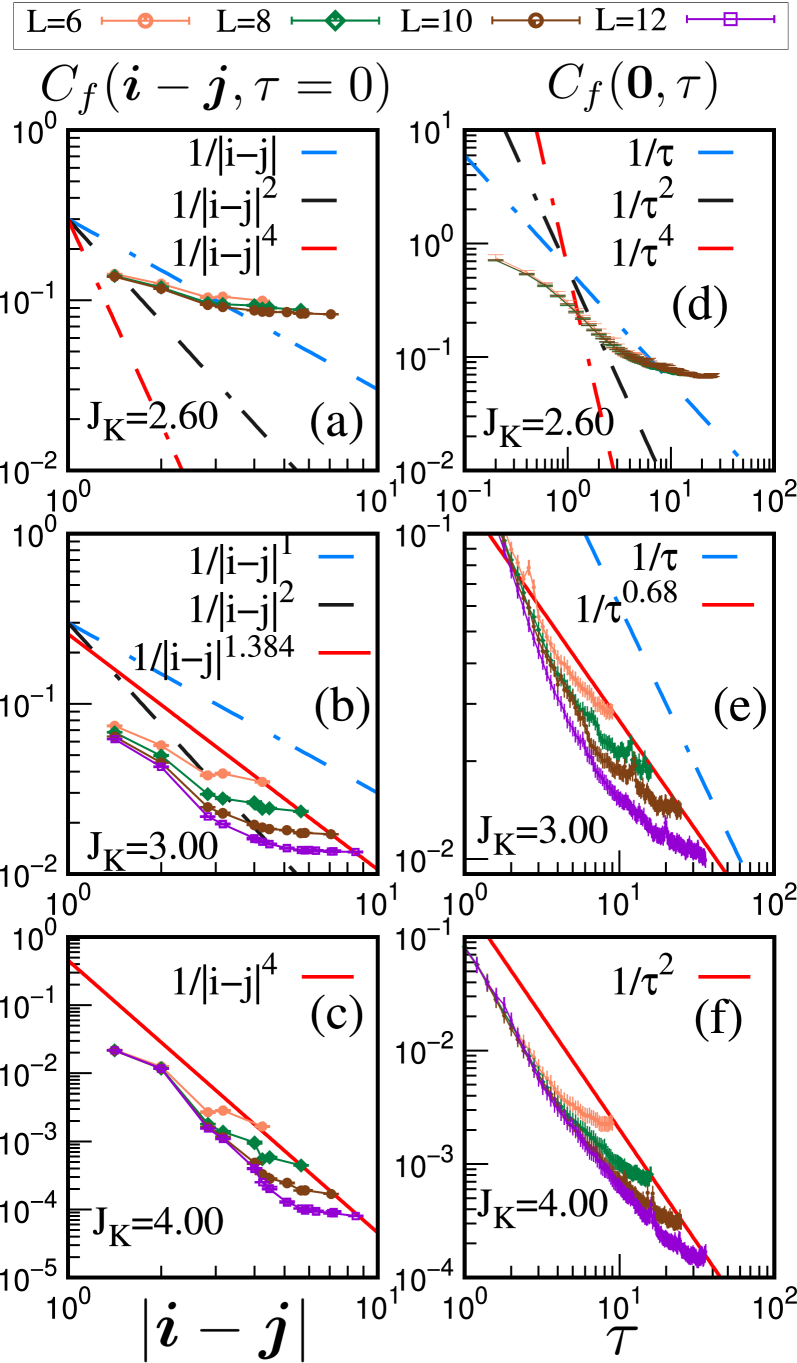
Figure 7: Spin-spin correlations $C_{f}(\boldsymbol{i}-\boldsymbol{j},\tau)$ in impurity layer as function of distance $r$ at equal time $\tau=0$ (left column) and imaginary time $\tau$ at equal position $r=0$ (right column) for different values of $J_{\mathrm{K}}$ in the antiferromagnetic phase (top row), quantum critical regime (center row), and paramagnetic heavy-fermion phase (bottom row), from finite-temperature QMC, using $\beta=L^{2}/2$. Dashed blue, black, and red lines represent power-law decay functions $f(x)\sim 1/x$, $1/x^{2}$ and $1/x^{4}$ for reference. The red solid line at (b)(c)(e)(f) represent the numerical fitting of the QMC data.

Following the weak-coupling-limit discussion and the observation of Landau damping in the dynamical spin structure factor, we foresee that the dynamical exponent is given by $z=2$ at the magnetic critical point $J_{\mathrm{K}}^{\mathrm{c}}$. Since the dynamical exponent encodes the asymmetry between space and time, we consider real-space equal-time spin correlations $C_{f}(\boldsymbol{i}-\boldsymbol{j},\tau=0)$ in Figs. 7(a)-(c), as well as local time-displaced correlations $C_{f}(\boldsymbol{0},\tau)$ in Figs. 7(d)-(f). Here,

$$C_{f}(\boldsymbol{i}-\boldsymbol{j},\tau)=\left\langle\hat{S}_{\boldsymbol{i}}^{f}(\tau)\hat{S}_{\boldsymbol{j}}^{f}(0)\right\rangle.$$ (28)

For this set of calculations, we have used the finite-temperature code with $\beta=L^{2}/2$ so as to observe ground-state properties. At $J_{\mathrm{K}}=2.60<J_{\mathrm{K}}^{\mathrm{c}}$, Figs. 7(a,d), the Heisenberg model has long-range order, such that the spin correlations saturate to a constant both in space and imaginary time. We note that our simulations explicitly preserve SU(2) spin symmetry, so that we cannot distinguish between longitudinal and transverse modes. In other words, the data of Figs. 7(a,d) are dominated by the long-range order, and we are blind to the transverse critical modes.

At the critical point $J_{\mathrm{K}}=3.00\approx J_{\mathrm{K}}^{\mathrm{c}}$, Figs. 7(b,e), the data suggest power-law decays of the form $C_{f}(\boldsymbol{i}-\boldsymbol{j},\tau=0)\propto 1/|\boldsymbol{i}-\boldsymbol{j}|^{\alpha_{r}}$ and $C_{f}(\boldsymbol{0},\tau)\propto 1/\tau^{\alpha_{t}}$, respectively. By performing a numerical fit, we have extracted the values of the exponents, resulting in $\alpha_{r}=1.384(2)$ and $\alpha_{t}=0.68(2)$, satisfying $\alpha_{r}=2\alpha_{t}$ within numerical uncertainty, consistent with $z=2$ at the critical point. The fits are represented as solid red lines in Figs. 7(b,e).

Finally, in the paramagnetic heavy-fermion phase, Figs. 7(c,f), the spin-spin correlations inherit the scaling of the host metal. That is, $C_{f}(\boldsymbol{i}-\boldsymbol{j},\tau=0)\propto 1/|\boldsymbol{i}-\boldsymbol{j}|^{4}$ in space and $C_{f}(\boldsymbol{0},\tau)\propto 1/\tau^{2}$ in imaginary time. We understand this from the point of view of the composite fermion operator,

$$\left\langle\hat{\boldsymbol{S}}_{\boldsymbol{i}}^{f}(\tau)\hat{\boldsymbol{S}}_{\boldsymbol{j}}^{f}(0)\right\rangle =\left\langle\frac{1}{2}\hat{\boldsymbol{f}}_{\boldsymbol{i}}^{\dagger}(\tau)\boldsymbol{\sigma}\hat{\boldsymbol{f}}_{\boldsymbol{i}}(\tau)\cdot\frac{1}{2}\hat{\boldsymbol{f}}_{\boldsymbol{j}}^{\dagger}(0)\boldsymbol{\sigma}\hat{\boldsymbol{f}}_{\boldsymbol{j}}(0)\right\rangle\allowdisplaybreaks[1]$$

$$=\left\langle\frac{1}{2}\boldsymbol{\tilde{f}}_{\boldsymbol{i}}^{\dagger}(\tau)\boldsymbol{\sigma}\boldsymbol{\tilde{f}}_{\boldsymbol{i}}(\tau)\cdot\frac{1}{2}\boldsymbol{\tilde{f}}_{\boldsymbol{j}}^{\dagger}(0)\boldsymbol{\sigma}\boldsymbol{\tilde{f}}_{\boldsymbol{j}}(0)\right\rangle.$$ (29)

In the paramagnetic heavy-fermion phase, the spin correlations are well understood by considering the bubble of the above particle-hole correlation function. In fact, in the large-$N$ limit, vertex contributions vanish, and as shown in Ref. [18] for the specific case of the half-filled two-dimensional Kondo lattice model, the large-$N$ saddle point is adiabatically connected to the SU(2) model. Since the $\boldsymbol{\tilde{f}}_{\boldsymbol{i}}(\tau)$ operator has the same quantum numbers as that of the electron operator, we expect it to have the same scaling dimension.

IV.3 Composite-fermion and conduction-electron spectral functions

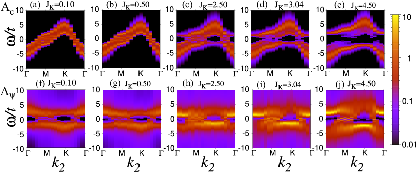
Figure 8: Fermion spectral functions $A_{c}(\boldsymbol{k}_{2},\omega)$ (top row) and $A_{\psi}(\boldsymbol{k}_{2},\omega)$ (bottom row) from finite-temperature QMC, using $\beta=40$ and $L=12$. The Kondo coupling $J_{\mathrm{K}}$ increases from left to right.

The composite-fermion spectral function is a very useful quantity to assess the presence of Kondo screening. Let us start with the corresponding periodic Anderson model. In this case, Kondo breakdown corresponds to an orbital-selective Mott transition [35], and the single-particle spectral function of the impurity-orbital fermion operator $\hat{d}^{\dagger}$ will show a gap. In the limit where charge fluctuations on the impurity orbitals are suppressed and the periodic Anderson model maps onto the Kondo lattice model, the composite fermion is nothing but the canonical Schrieffer-Wolff transformation of the $\hat{d}^{\dagger}$ operator. Hence, Kondo breakdown corresponds to an absence of spectral weight at the Fermi energy of the composite fermion operator.

In Fig. 8, we present the evolution of the $c$-fermion spectral function $A_{c}(\boldsymbol{k}_{2},\omega)$ and the composite-fermion spectral function $A_{\psi}(\boldsymbol{k}_{2},\omega)$ upon varying the Kondo coupling $J_{\mathrm{K}}$. At weak coupling, $J_{\mathrm{K}}=0.1$ and $J_{\mathrm{K}}=0.5$, the magnetic impurities exhibit long-range antiferromagnetic order. The $c$-fermion spectral function is very similar to the corresponding mean-field result. The composite-fermion spectral function $A_{\psi}(\boldsymbol{k}_{2},\omega)$ reveals a momentum shift of $\mathbb{Q}=(\pi,\pi)$ with respect to $A_{c}(\boldsymbol{k}_{2},\omega)$, see also Fig. 4(g). In addition, the intense composite-fermion spectral weight at $\omega\simeq 0$ at the $\boldsymbol{\Gamma}$ point suggests Kondo screening throughout the antiferromagnetic phase for all $J_{\mathrm{K}}>0$. This feature becomes clear by comparing Figs. 8(f,g) with the mean-field composite-fermion spectral function in the coexistence phase, Fig. 4(i).

As one enhances the Kondo coupling into the finite-temperature quantum critical fan, $J_{\mathrm{K}}=2.50$ and $J_{\mathrm{K}}=3.04$, we observe growing (decreasing) low-energy spectral weight in the composite-fermion ($c$-electron) spectral function. Due to the reduction of the antiferromagnetic order parameter, band folding features in the composite-fermion spectral function become weaker as compared to smaller values of $J_{\mathrm{K}}$.

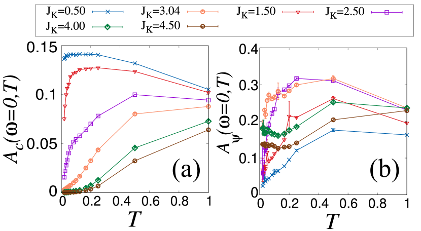
Figure 9: Local density of states $A_{c}(\omega=0)$ (left) and $A_{\psi}(\omega=0)$ (right) near the Fermi level as function of temperature $T=1/\beta$ for different values of $J_{\mathrm{K}}$ from finite-temperature QMC. Here, we consider $L=10$ and restrict the data to the temperature range with smallest finite-size effects.

At large Kondo coupling, $J_{\mathrm{K}}=4.50$, deep in the paramagnetic heavy-fermion phase, magnetic correlations are short ranged and the $c$ fermion strongly hybridizes with the $f$ pseudo fermion. In Fig. 8(e), we observe that the low-energy $c$-fermion spectral weight is greatly suppressed. This is consistent with the mean-field result of Fig. 4(b). On the other hand, Fig. 8(j) shows that the composite fermion has substantial low-energy weight, again in accordance to the large-$N$ calculation of Fig. 4(h).

As mentioned at the beginning of this section, it is crucial to understand whether the $f$-fermion spectral function has finite spectral weight at the Fermi energy, since this a measure for Kondo screening. In Fig. 9, we present the temperature dependence of the local density states near the Fermi level $A_{c/{\psi}}(\omega=0,T)$ as function of temperature. Here we use the approximate relation $A_{c/{\psi}}(\omega=0)\approx\frac{\beta}{\pi N}\sum_{k_{2}}G_{c/{\psi}}\left(k_{2},\tau=\frac{\beta}{2}\right)$ to obtain this quantity directly, circumventing the need for analytical continuation. Note that for a smooth density of states at the Fermi level, this equation becomes exact in the low-temperature limit. At low temperatures, as presented in Fig. 9(a), the $c$-fermion local density of states, $A_{c}(\omega=0)$, decreases with growing Kondo coupling. When $J_{\mathrm{K}}>J_{\mathrm{K}}^{\mathrm{c}}$, $A_{c}(\omega=0)$ becomes very small at low temperatures. In contrast, the results for the composite-fermion local density of states $A_{\psi}(\omega=0)$, as shown in Fig. 9(b), suggest that this quantity does not vanish for any finite $J_{\mathrm{K}}$ in the zero-temperature limit. Since composite and $c$ fermions have the same quantum numbers, the supports of both spectral functions are expected to be identical. However, the spectral weight can differ substantially. Hence, we understand that the low-energy spectral weight of the conduction electrons deep in the paramagnetic heavy-fermion phase does not vanish. Further data, demonstrating that these results are representative of the thermodynamic limit, are provided in Appendix C.

On the whole, the results shown in this section provide numerical evidence of a metal-to-metal magnetic transition across which Kondo screening does not break down.

V Conclusions and outlook

The model of the Kondo heterostructure presented in this work provides a unique possibility to numerically investigate the physics of quantum spins in a metallic environment without encountering the infamous negative-sign problem. The model can be seen as a dimensional generalization of a spin-chain on a metallic surface [10, 11], leading to a two-dimensional quantum antiferromagnet embedded in a three-dimensional metal. Our model is relevant for the description of Kondo heterostructures such as CeIn₃/LaIn₃ superlattices studied experimentally in Ref. [12].

Combining a weak-coupling analysis and a mean-field calculation, we foresee the existence of a magnetic quantum critical point in a metallic environment driven by the Kondo interaction. This is confirmed by unbiased large-scale auxiliary-field QMC simulations. The antiferromagnetic heavy-fermion phase is characterized by Landau-damped Goldstone modes and the quantum critical point is consistent with a dynamical exponent $z=2$. Both aspects are a direct consequence of the metallic environment. In the paramagnetic heavy-fermion phase, the spin correlations of the magnetic system inherit those of the host metal, in accordance with the large-$N$ calculation. This result can be understood in terms of the emergence of a composite fermion operator that carries the quantum number of the electron and hence possesses the same scaling dimension. Within a U(1) gauge theory of the Kondo lattice, the composite fermion corresponds to the bound state of the Abrikosov pseudo fermion and the phase of the bosonic hybridization field.

Of crucial importance for the understanding of the transition is the fate of the aforementioned composite fermion and the associated Kondo effect. In fact, up to the smallest Kondo coupling we considered, $J_{\mathrm{K}}=0.1$, the composite-fermion spectral function does not develop a gap, such that we can exclude Kondo breakdown. We note that Kondo breakdown within the magnetically-ordered phase would not violate Luttinger’s theorem due to the doubling of the magnetic unit cell [36]. Hence, the quantum critical point in our model describes an interesting metal-to-metal magnetic transition in a model with SU(2) local spins, in which the heavy-fermion quasiparticle does neither disintegrate at the transition nor in the magnetic phase. Consequently, this transition falls into the category of Hertz-Millis [37, 38], albeit with the important property that only the two-dimensional crystal momentum is conserved up to a reciprocal lattice vector. The understanding of this transition and a possible non-Fermi liquid character is left for future work. Another intriguing issue is the finite-temperature phase diagram. In the very same way that dissipation stabilizes long-range order in the ground state of a one-dimensional spin-chain [39], one might expect the Kondo heterostructure to show magnetism at finite temperature.

Appendix A Numerical solution of self-consistency equations

In the mean-field analysis, we employ the standard iterative method to solve the self-consistency equations, Eq. (21). We denote the set of mean-field parameters at the $n$-th step of the iteration as $x_{n}$, with $n\in\mathbb{N}$. The iterative method starts with an initial guess of the mean-field order parameters $x_{1}=(m_{c,1},m_{f,1},V_{1})$. At each step of the iteration, we compute the single-particle Green’s function by diagonalising the mean-field Hamiltonian $\hat{H}_{\text{MF}}$, Eq. (20), with input parameters $x_{n}$. The convergence is determined using a quantity $\rho^{2}_{n}$, defined as

$$\rho^{2}_{n}=\rho_{c,n}^{2}+\rho^{2}_{f,n}+\rho^{2}_{V,n},$$ (30)

where

$$\rho_{c,n} =m_{c,n}+\frac{1}{2L^{2}}\sum_{\boldsymbol{k}_{2},\sigma}\left(-1\right)^{\sigma}$$

$$\quad\times\left\langle\hat{c}_{\boldsymbol{k}_{2}+\boldsymbol{Q},R_{z}=0,\sigma}^{\dagger}\hat{c}_{\boldsymbol{k}_{2},R_{z}=0,\sigma}^{\phantom{\dagger}}\right\rangle_{n},$$ (31)

$$\rho_{f,n} =m_{f,n}-\frac{1}{2L^{2}}\sum_{\boldsymbol{k}_{2},\sigma}\left(-1\right)^{\sigma}\left\langle\hat{f}_{\boldsymbol{k}_{2}+\boldsymbol{Q},\sigma}^{\dagger}\hat{f}_{\boldsymbol{k}_{2},\sigma}^{\phantom{\dagger}}\right\rangle_{n},$$ (32)

$$\rho_{V,n} =V_{n}-\frac{1}{2L^{2}}\sum_{\boldsymbol{k}_{2},\sigma}\left\langle\hat{c}_{\boldsymbol{k}_{2},R_{z}=0,\sigma}^{\dagger}\hat{f}_{\boldsymbol{k}_{2},\sigma}^{\phantom{\dagger}}+\text{h.c.}\right\rangle_{n},$$ (33)

where $\langle\dots\rangle_{n}$ denotes expectation value with respect to $\hat{H}_{\text{MF}}$ at the $n$-th step of the iteration, i.e., with input parameters $x_{n}$. If $\rho^{2}_{n}$ is larger than or equal to a small threshold value $r\ll 1$, the algorithm proceeds to the next iteration, and we update the mean-field parameters $x_{n+1}$ according to Eq. (21), using the Green’s function obtained in the previous step. For $\rho^{2}_{n}<r$, we have obtained a fixed-point solution $x_{n}$ with a precision of $r$. In our analysis, we set the threshold value of $r$ to $10^{-10}$, which is sufficient for a system size of $L=100$.

Appendix B Twisted boundary conditions in $z$ direction

For periodic boundary conditions, the fermion operator satisfies $\hat{c}_{\boldsymbol{r}+\boldsymbol{L}_{a}}=\hat{c}_{\boldsymbol{r}}$, where $a=1,2,3$ represents the $x,y,z$ directions. For twisted boundary conditions along the $z$ direction, the condition transforms into $\hat{c}_{\boldsymbol{r}+\boldsymbol{L}_{a}}=e^{2\pi i\Phi/\Phi_{0}\delta_{a,z}}\hat{c}_{\boldsymbol{r}}$. The twist in the boundary can be removed at the expense of a vector potential in the Hamiltonian that can be locally but not globally removed with a gauge transformation [40]. Specifically we can consider the canonical transformation:

$$\tilde{d}_{\boldsymbol{r}}=e^{-\frac{2\pi i\Phi}{\Phi_{0}}\frac{\boldsymbol{e}_{z}\cdot\boldsymbol{r}}{L}}\tilde{c}_{\boldsymbol{r}}.$$ (34)

$\tilde{d}_{\boldsymbol{r}}$ satisfies periodic boundary conditions,

$$\tilde{d}_{\boldsymbol{r}+\boldsymbol{L}_{a}}=\tilde{d}_{\boldsymbol{r}}$$ (35)

and the hopping part of our Hamiltonian transforms to:

$$\hat{H}_{\text{Fermi}}=-t\sum_{\langle\boldsymbol{r},\boldsymbol{r}^{\prime}\rangle}\hat{d}^{\dagger}_{\boldsymbol{r}}e^{\frac{2\pi i\Phi}{\Phi_{0}}\frac{\left(\boldsymbol{r}-\boldsymbol{r}^{\prime}\right)\cdot\boldsymbol{e}_{z}}{L}}\hat{d}^{\phantom{\dagger}}_{\boldsymbol{r}^{\prime}}$$ (36)

Fourier transform gives:

$$\hat{H}_{\text{Fermi}}=\sum_{\boldsymbol{k}}\left[-2t\sum_{a=1}^{3}\cos\left(k_{a}+\delta_{a,3}\frac{\Phi}{\Phi_{0}}\frac{2\pi}{L}\right)\right]\hat{d}_{\boldsymbol{k}}^{\dagger}\hat{d}_{\boldsymbol{k}}.$$ (37)

In the QMC calculation, we obtain the observable by averaging over different twisted boundary condition $\Phi/\Phi_{0}\in\left[0,1\right]$ to reduce finite-size effects. In particular for a one-dimensional non-interacting system it was pointed out in Ref. [31] such an averaging over boundary conditions yields exact results for any value of $L$.

Hence, for a given operator $\hat{O}$, we evaluate:

$$\left\langle\hat{O}\right\rangle=\int_{0}^{1}d\Phi\left\langle\hat{O}\left(\Phi\right)\right\rangle.$$ (38)

This strategy improve the data quality in the free fermion system by increasing the momentum resolution for finite system sizes. In Fig. 10, we provide a simple benchmark of the noninteracting $c$-fermion Green’s function at the impurity layer, obtained from $\hat{H}_{\text{Fermi}}$, defined as

$$G^{R_{z}=0}_{c,0}(\boldsymbol{k}_{2},\omega_{n})=-\int_{0}^{\beta}d\tau\,e^{i\omega_{n}\tau}\left\langle\hat{c}_{\boldsymbol{k}_{2},R_{z}=0}(\tau)\hat{c}_{\boldsymbol{k}_{2},R_{z}=0}^{\dagger}(0)\right\rangle_{0}$$ (39)

where $\omega_{n}=(2n+1)\pi/\beta$ is the Matsubara frequency. By considering Eq. (36) in continuous momentum space, $G^{R_{z}=0}_{c,0}(\boldsymbol{k}_{2},\omega_{n})$ follows the analytic form given in Eq. (46), see the green line in Fig. 10. In the lattice calculation, this quantity suffers from the finite momentum resolution and deviates from the analytic form at low frequency, which is well observed for periodic boundary conditions, shown in purple in Fig.10. The orange dots shown in Fig. 10 represent the results of finite-size lattice calculations with twisted boundary conditions. In this calculation, we average over ten different twists, satisfying $\Phi/\Phi_{0}=0.1n$ for $n\in[0,1,\dots,9]$. As presented in Fig.10, the mismatch between the finite-size calculation and the analytic form of $G^{R_{z}=0}_{c}(\boldsymbol{k}_{2},\omega_{n})$ at low frequency can be reduced effectively by using twisted boundary conditions, at least in the noninteracting system. On this ground, we believe this technique can alleviate finite-size effects also in the interacting system.

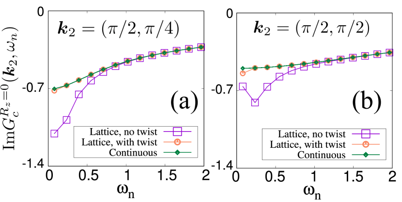
Figure 10: Imaginary part of $c$-fermion Green’s function $\text{Im}\,G_{c}^{R_{z}=0}(\boldsymbol{k}_{2},\omega_{n})$ as function of Matsubara frequency $\omega_{n}=(2n+1)\pi/\beta$ for (a) $\boldsymbol{k}_{2}=(\pi/2,\pi/4)$ and (b) $\boldsymbol{k}_{2}=(\pi/2,\pi/2)$. Green dots follow Eq. (46). Purple (orange) dots are obtained from finite-size lattice calculations with linear size $L=8$ and inverse temperature $\beta=40$ with periodic boundary conditions (twisted boundary conditions, averaged over ten different twists). Lines represent guides to the eye.

Appendix C Finite-size effects on local density of states

In this appendix, we provide additional plots for the local density of states $A_{c/\psi}(\omega=0,T)$, in order to illustrate the finite-size effects. In Figs. 11 and 12, we compare the data obtained from different system sizes, using different values of the Kondo coupling $J_{\mathrm{K}}$. For the considered range of parameters, $T>0.025$, $J_{\mathrm{K}}>0.1$, lattices with linear system sizes $L\geq 10$ appear to be representative of the thermodynamic limit.

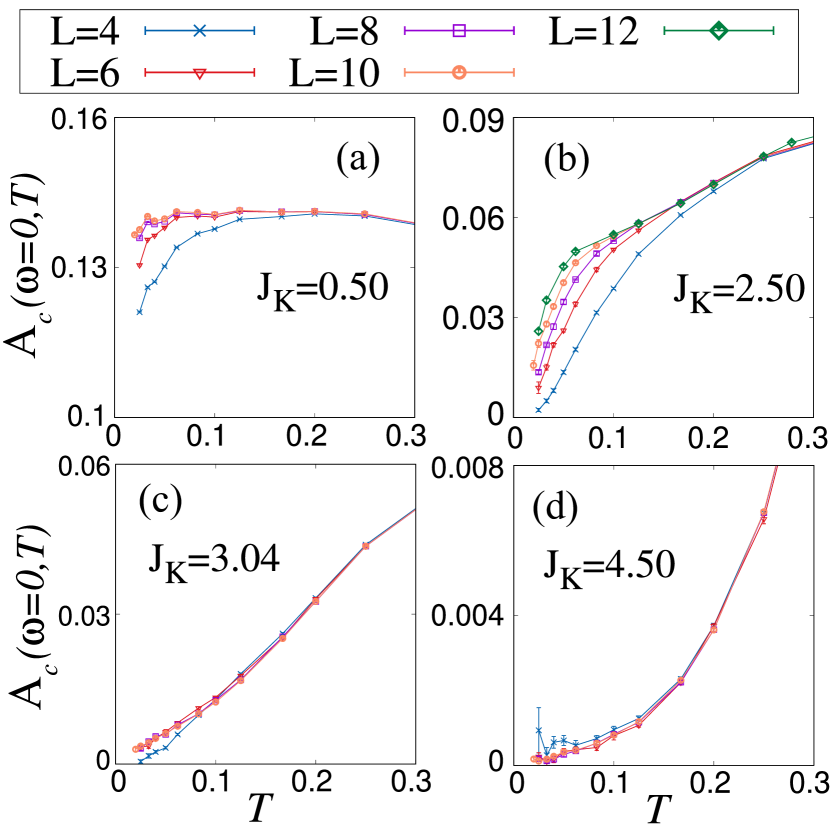
Figure 11: Conduction-electron local density of states $A_{c}(\omega=0,T)$ near the Fermi level as function of temperature $T$ for different lattice sizes $L$. In each panel, different colors indicate different system sizes. The Kondo coupling $J_{\mathrm{K}}$ increases from left to right and top to bottom.

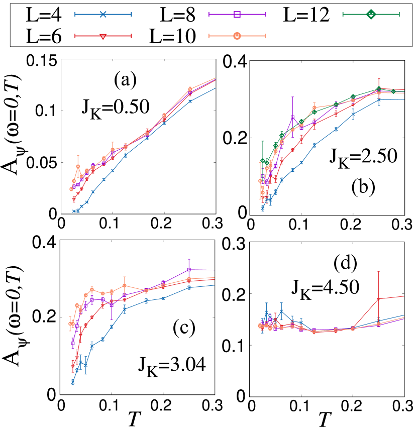
Figure 12: Same as Fig. 11, but for the composite-fermion local density of states $A_{\psi}(\omega=0,T)$.

Appendix D Spin-wave theory in antiferromagnetic phase

To confirm the existence of Landau-damped Goldstone modes in the antiferromagnetic phase within a spin-wave description, we perform a Holstein-Primakoff transformation of the local moments. The latter are then perturbatively coupled to the conduction electrons. From a theoretical perspective, this procedure provides a combined expansion in both the inverse spin lengths of the local moments $1/S$ and the Kondo coupling $J_{\mathrm{K}}$. In particular, if the magnon modes can dissipate energy by exciting electrons, this is reflected in the magnon propagator, which we will compute in the following.

In the absence of Kondo interactions, the local moments form a Heisenberg antiferromagnet in the impurity layer. We introduce two sublattices $A$ and $B$ to take the staggered magnetization into account. The leading order of the Holstein-Primakoff transformation in the limit $S\to\infty$ reads

$$\begin{split}\begin{array}[]{ l l}\hat{{S}}^{+}_{\boldsymbol{i}\in A}\simeq\sqrt{2S}a_{\boldsymbol{i}}&\hat{{S}}^{+}_{\boldsymbol{i}\in B}\simeq\sqrt{2S}b^{\dagger}_{\boldsymbol{i}}\\ \hat{{S}}^{-}_{\boldsymbol{i}\in A}\simeq\sqrt{2S}a^{\dagger}_{\boldsymbol{i}}&\hat{{S}}^{-}_{\boldsymbol{i}\in B}\simeq\sqrt{2S}b_{\boldsymbol{i}}\\ \hat{{S}}^{z}_{\boldsymbol{i}\in A}=S-a^{\dagger}_{\boldsymbol{i}}a_{\boldsymbol{i}}&\hat{{S}}^{z}_{\boldsymbol{i}\in B}=-S+b^{\dagger}_{\boldsymbol{i}}b_{\boldsymbol{i}}\end{array}\,,\end{split}$$ (40)

where the bosonic operators $a^{(\dagger)}_{\boldsymbol{i}},b^{(\dagger)}_{\boldsymbol{i}}$ annihilate (create) a spin-wave excitation. To consider the coupling between these magnons and the conduction electrons, we first have to establish a description of the full three-dimensional electronic band structure that is compatible with the Néel order in the impurity layer at $R_{z}=0$. To this end, we formally introduce the same $A,B$ sublattices in all layers with $A-A$ stacking in the $R_{z}$ direction, such that hopping processes between layers with different $R_{z}$, but identical in-plane coordinate $\boldsymbol{i}$, do not change the sublattice type. This reformulation is equivalent to considering a square lattice in each layer with a basis that contains two neighboring sites of the original lattice. Like in a two-dimensional system, the corresponding band structure is therefore obtained by backfolding the in-plane part of the dispersion relation $\epsilon_{\boldsymbol{k}_{2},k_{z}}$ with $\boldsymbol{Q}$, see Fig. 13(a). This gives rise to the two new bands

$$\epsilon^{(1,2)}_{\boldsymbol{k}_{2},k_{z}} =\mp 2t(\cos k_{x}+\cos k_{y})-2t\cos k_{z}=\pm\epsilon_{\boldsymbol{k}_{2}}+\epsilon_{k_{z}}\,.$$ (41)

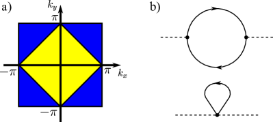
Figure 13: (a) Crystallographic Brillouin zone (blue) and backfolded magnetic Brilliouin zone (yellow). (b) Magnon self-energies $\pi$ in one-loop perturbation theory from Eqs. (50) (top) and (51) (bottom).

In this way, $\hat{H}_{\mathrm{Fermi}}$ from Eq. (II) becomes

$$\hat{H}_{\mathrm{Fermi}}=\sum_{\begin{subarray}{c}\boldsymbol{k}_{2},k_{z},\sigma\\ n=1,2\end{subarray}}\epsilon^{(n)}_{\boldsymbol{k}_{2},k_{z}}\hat{c}_{\boldsymbol{k}_{2},k_{z},n,\sigma}^{\dagger}\hat{c}_{\boldsymbol{k}_{2},k_{z},n,\sigma}^{\phantom{\dagger}}.$$ (42)

and consequently, also the associated bare propagator acquires a matrix form in the band space with indices $n_{1,2}=1,2$

$$(\underline{G}^{(0)})_{n_{1},n_{2},k_{z},q_{z},\sigma}(\boldsymbol{k}_{2},\omega)=\left(\begin{array}[]{c c}\frac{\delta_{k_{z}q_{z}}}{i\omega-\epsilon^{(1)}_{\boldsymbol{k}_{2},k_{z}}}&\underline{0}\\ \underline{0}&\frac{\delta_{k_{z}q_{z}}}{i\omega-\epsilon^{(2)}_{\boldsymbol{k}_{2},k_{z}}}\end{array}\right)\,,$$ (45)

where the matrix structure in the out-of-plane momentum space has been introduced, anticipating the violation of momentum conservation by the interactions. In analogy to the main text, we define the local propagators at $R_{z}=0$, $g^{(0)}_{n_{1},n_{2},\sigma}(\boldsymbol{k}_{2},\omega)=1/L\sum_{k_{z},q_{z}}(\underline{G}^{(0)})_{n_{1},n_{2},k_{z},q_{z},\sigma}(\boldsymbol{k}_{2},\omega)$. For the tight-binding dispersion considered here, one has

$$g^{(0)}_{n_{1},n_{2},\sigma}(\boldsymbol{k}_{2},\omega)=\frac{\delta_{n_{1},n_{2}}}{\sqrt{(i\omega-\epsilon_{\boldsymbol{k}_{2}}+2t)}\sqrt{(i\omega-\epsilon_{\boldsymbol{k}_{2}}-2t)}}\,.$$ (46)

Next, we turn to the perturbative corrections arising from $\hat{H}_{\rm{Kondo}}$ given in Eq. (5). The most important term is of order $\mathcal{O}(SJ_{\mathrm{K}})$ and describes the interaction with the static staggered magnetization contained in the $\hat{S}^{z}$ components of Eq. (40). The corresponding mean-field-like Hamiltonian reads

$$H_{\text{MF}}=-\frac{J_{\mathrm{K}}S}{2L}\sum_{\boldsymbol{k}_{2},k_{z},q_{z},\sigma}\sigma\left(c^{\dagger}_{\boldsymbol{k}_{2},k_{z},\sigma,1}c_{\boldsymbol{k}_{2},q_{z},\sigma,2}+\text{h.c.}\right)\,,$$ (47)

where spin up (down) correspond to the value $\sigma=\pm 1$. Since the perturbation is quadratic, it gives rise to the static self-energy $(\underline{\Sigma}^{\text{MF}})_{n_{1},n_{2},k_{z},q_{z},\sigma}=\tilde{\Sigma}^{\text{MF}}_{n_{1},n_{2},k_{z},q_{z},\sigma}/L=-\sigma J_{\mathrm{K}}S(1-\delta_{n_{1},n_{2}})/(2L)$, which is independent of momentum. The fact that the self-energy is nonzero only for interband processes stems from the staggered magnetization: Any scattering event from the alternating pattern translates to a shift by $\boldsymbol{Q}$ in momentum space that connects identical wave vectors, but changes the band index. Note that $\underline{\Sigma}^{\text{MF}}$ is equivalent to the mean-field form discussed above Eq. (22), with the additional simplification that in the perturbative regime the staggered magnetization is given by $m^{f}=S$. The solution to the Dyson equation $[\underline{G}^{\text{MF}}]^{-1}=\underline{[}G^{(0)}]^{-1}-\underline{\Sigma}^{\text{MF}}$ is given in terms of the scattering form

$$\begin{split}&\underline{G}_{\sigma}^{\text{MF}}(\boldsymbol{k}_{2},\omega)=\\ &\qquad\underline{G}_{\sigma}^{(0)}(\boldsymbol{k}_{2},\omega)+\underline{G}_{\sigma}^{(0)}(\omega,\boldsymbol{k}_{2})\cdot\underline{T}_{\sigma}^{\text{MF}}(\boldsymbol{k}_{2},\omega)\cdot\underline{G}_{\sigma}^{(0)}(\boldsymbol{k}_{2},\omega)\,,\end{split}$$ (48)

where the dots denote matrix multiplication both in band and $k_{z}$ space, and the $T$ matrix is given at the mean-field level by

$$\begin{split}&\underline{T}_{\sigma}^{\text{MF}}(\boldsymbol{k}_{2},\omega)=\frac{1/L}{1-(SJ_{\mathrm{K}}/2)^{2}g^{(0)}_{11,\sigma}(\boldsymbol{k}_{2},\omega)g_{22,\sigma}^{(0)}(\boldsymbol{k}_{2},\omega)}\\ &\times\left(\begin{array}[]{c c}(SJ_{\mathrm{K}}/2)^{2}g^{(0)}_{22,\sigma}(\boldsymbol{k}_{2},\omega)\underline{A}&-\sigma SJ_{\mathrm{K}}/2\cdot\underline{A}\\ -\sigma SJ_{\mathrm{K}}/2\cdot\underline{A}&(SJ_{\mathrm{K}}/2)^{2}g^{(0)}_{11,\sigma}(\boldsymbol{k}_{2},\omega)\underline{A}\end{array}\right)\,.\end{split}$$ (49)

As in Eq. (45), the outer $2\times 2$ matrix refers to the band index, whereas the out-of-plane momentum structure for $L$ layers is incorporated by the inner $L\times L$ matrices proportional to $\underline{A}$. Since the Kondo interaction is localized in only of the layers, $H_{\text{MF}}$ does not introduce correlations between the initial and final out-of-plane momenta, and we have $(\underline{A})_{k_{z},q_{z}}=1$ for all $k_{z},q_{z}$. Physically, $\underline{T}^{\text{MF}}_{\sigma}$ can be understood as the $T$ matrix that arises from scattering a single particle off a $\delta$ potential of strength $-\sigma SJ_{\mathrm{K}}$. However, even (odd) powers of $J_{\mathrm{K}}$ appear in the diagonal (off-diagonal) terms, because a single scattering event changes the band index. Note that $\underline{G}_{\sigma}^{\text{MF}}$ includes all orders of $S$ and $J_{\mathrm{K}}$, which turns out crucial in order to perform a consistent expansion.

Next, we have to consider the perturbative interaction terms from $H_{\rm{Kondo}}$ that contain magnon fields. From the Holstein-Primakoff transformation (40) of the spin components $S^{x,y}_{\boldsymbol{i}}$, one obtains a Hamiltonian that is linear in the magnons and involves spin flips in the electron sector,

$$\begin{split}H_{1}\!=\frac{J_{\mathrm{K}}\sqrt{S}}{2L}\!\!\!&\sum_{\begin{subarray}{c}\boldsymbol{p}_{2},\boldsymbol{q}_{2}\\ n=1,2\end{subarray}}\!\!\!\left[(c^{\dagger}_{\boldsymbol{q}_{2}-\boldsymbol{p}_{2},R_{z}=0,\uparrow,n}c_{\boldsymbol{q}_{2},R_{z}=0,\downarrow,n})(a^{\dagger}_{\boldsymbol{p}_{2}}+b_{-\boldsymbol{p}_{2}})\right.\\ &\left.+(c^{\dagger}_{\boldsymbol{q}_{2}-\boldsymbol{p}_{2},R_{z}=0,\uparrow,n}c_{\boldsymbol{q}_{2},R_{z}=0,\downarrow,\bar{n}})(b_{-\boldsymbol{p}_{2}}-a^{\dagger}_{\boldsymbol{p}_{2}})+\rm{h.c.}\right]\!.\end{split}$$ (50)

Here, $\bar{n}$ denotes the complementary value of $n$ in band space, i.e., if $n=1$, then $\bar{n}=2$, and vice versa. In other words, the first line describes intraband and the second line interband processes. In addition, we have the two-magnon terms from the $\mathcal{O}(S^{0})$ contribution to $S^{z}_{\boldsymbol{i}}$ in Eq. (40):

$$\begin{split}H_{2}\!=\!\frac{\sigma J_{\mathrm{K}}}{2L^{2}}\!\!\!\!\!&\sum_{\begin{subarray}{c}\boldsymbol{q}_{2},\boldsymbol{p}_{2},\boldsymbol{l}_{2}\\ \sigma,n=1,2\end{subarray}}\!\!\!\!\!\left[\!(c^{\dagger}_{\boldsymbol{q}_{2}+\boldsymbol{l}_{2}-\boldsymbol{p}_{2},R_{z}=0,\sigma,n}c_{\boldsymbol{q}_{2},R_{z}=0,\sigma,n}\!)(b^{\dagger}_{\boldsymbol{p}_{2}}b_{\boldsymbol{l}_{2}}\!\!-\!a^{\dagger}_{\boldsymbol{p}_{2}}a_{\boldsymbol{l}_{2}})\right.\\ &\left.+(c^{\dagger}_{\boldsymbol{q}_{2}+\boldsymbol{l}_{2}-\boldsymbol{p}_{2},R_{z}=0,\sigma,n}c_{\boldsymbol{q}_{2},R_{z}=0,\sigma,\bar{n}})(a^{\dagger}_{\boldsymbol{p}_{2}}a_{\boldsymbol{l}_{2}}+b^{\dagger}_{\boldsymbol{p}_{2}}b_{\boldsymbol{l}_{2}})\right].\end{split}$$ (51)

To incorporate the effects of $H_{1,2}$ properly via perturbation theory, we use a coherent-state path integral formulation and integrate out the conduction electrons. This yields the effective partition function $\mathcal{Z}=\int\mathcal{D}[a,b]\exp(-S[a,b])$ of the magnons. In particular, the quadratic part of the action $S[a,b]$ acquires self-energy corrections by the Kondo interactions but the condition $\langle a_{\boldsymbol{p}_{2}}\rangle=0=\langle b_{\boldsymbol{p}_{2}}\rangle$ is retained since the mean-field expectation value of the staggered magnetization remains unchanged. The dressed quadratic magnon action reads

$$S[a,b]=\int\frac{d\Omega}{2\pi}\sum_{\boldsymbol{p}_{2}}\left(\begin{array}[]{c}a^{\ast}_{\boldsymbol{p}_{2},\Omega}\\ b_{-\boldsymbol{p}_{2},-\Omega}\end{array}\right)\underline{D}^{-1}(\Omega,\boldsymbol{p}_{2})\left(\begin{array}[]{c}a_{\boldsymbol{p}_{2},\Omega}\\ b^{\ast}_{-\boldsymbol{p}_{2},-\Omega}\end{array}\right),$$ (56)

where

$$\underline{D}^{-1}=\left(\begin{array}[]{c c}-i\Omega+\mathcal{E}_{\mathrm{H}}-\pi_{a^{\ast}a}(\boldsymbol{p}_{2},\Omega)&\mathcal{E}_{\mathrm{H}}\gamma_{\boldsymbol{p}_{2}}^{\ast}-\pi_{a^{\ast}b^{\ast}}(\boldsymbol{p}_{2},\Omega)\\ \mathcal{E}_{\mathrm{H}}\gamma_{\boldsymbol{p}_{2}}-\pi_{ba}(\boldsymbol{p}_{2},\Omega)&i\Omega+\mathcal{E}_{\mathrm{H}}-\pi_{bb^{\ast}}(\boldsymbol{p}_{2},\Omega)\end{array}\right).$$ (59)

Here, the contributions at vanishing $J_{\mathrm{K}}$ that stem from the Heisenberg Hamiltonian are encoded in $\mathcal{E}_{\mathrm{H}}=J_{\mathrm{H}}Sz_{\text{c}}$, with coordination number $z_{\text{c}}$ and $\gamma_{\boldsymbol{p}_{2}}=2(\cos p_{x}+\cos p_{y})/z_{\text{c}}$. In contrast, the $\pi_{ab}$ functions include the effects from the Kondo interactions. The lowest-order self-energies generated by $H_{1}$ and $H_{2}$ are depicted in Fig. 13(b), in which the internal electron lines are to be evaluated using $\underline{G}^{\text{MF}}$.

For the remaining part of this appendix, we assume the limits of large $S$ and small $J_{\mathrm{K}}$ in a way that the product $J_{\mathrm{K}}S$ remains small. As a result, the the particle-hole bubbles, which are generated by $H_{1}^{2}\sim J_{\mathrm{K}}^{2}S$, can be evaluated with $\underline{G}^{(0)}$, since the next-to-leading term from the $T$ matrix in $\underline{G}^{\text{MF}}$ is suppressed by an additional factor $J_{\mathrm{K}}S$. Therefore, the corresponding self-energies result in noninteracting local density-density correlation functions,

$$\begin{split}&\pi^{(1)}_{a^{\ast}a}(\boldsymbol{p}_{2},\Omega)=-\frac{J_{\mathrm{K}}^{2}S}{4}\sum_{n_{1},n_{2}=1,2}\Pi^{(0)}_{n_{1},n_{2}}(\boldsymbol{p}_{2},\Omega)\,,\\ &\pi^{(1)}_{a^{\ast}b^{\ast}}(\boldsymbol{p}_{2},\Omega)=-\frac{J_{\mathrm{K}}^{2}S}{4}\sum_{n_{1},n_{2}=1,2}(-1)^{n_{1}-n_{2}}\Pi^{(0)}_{n_{1},n_{2}}(\boldsymbol{p}_{2},\Omega)\,,\end{split}$$ (60)

and furthermore we have $\pi^{(1)}_{bb^{\ast}}(\boldsymbol{p}_{2},\Omega)=\pi^{(1)}_{a^{\ast}a}(\boldsymbol{p}_{2},\Omega)$ and $\pi^{(1)}_{ba}(\boldsymbol{p}_{2},\Omega)=\pi^{(1)}_{a^{\ast}b^{\ast}}(\boldsymbol{p}_{2},\Omega)$. In the above, the band-selective correlation functions read

$$\begin{split}\Pi^{(0)}_{nl}(\boldsymbol{p}_{2},\Omega)\!=\!\!\int\!\!\!\frac{d^{2}q_{2}}{(2\pi)^{2}}\!\!\int\!\!\!\frac{d\omega}{2\pi}g^{(0)}_{nn\uparrow}(\boldsymbol{q}_{2}+\boldsymbol{p}_{2},\omega+\Omega)g^{(0)}_{ll\downarrow}(\boldsymbol{q}_{2},\omega).\end{split}$$ (61)

Before evaluating them, we consider the perturbative correction from $H_{2}$ that gives rise to the fermion loop formed by a single $\underline{G}^{\text{MF}}$, yielding the constant

$$\begin{split}&\pi^{(2)}_{a^{\ast}a}(\boldsymbol{p}_{2},\Omega)=\\ &\frac{J_{\mathrm{K}}}{2L^{3}}\int\frac{d\omega}{(2\pi)}\sum_{\begin{subarray}{c}\boldsymbol{k}_{2},k_{z},q_{z}\\ \sigma,n_{1},n_{2}\end{subarray}}(-1)^{n_{1}-n_{2}}\sigma(\underline{G}^{\text{MF}}_{\sigma}(\boldsymbol{k}_{2},\omega))_{n_{1},n_{2},k_{z},q_{z}}\\ &\quad\qquad\qquad\simeq\frac{J_{\mathrm{K}}^{2}S}{2}\left[\Pi^{(0)}_{12}(\boldsymbol{0},0)+\Pi^{(0)}_{21}(\boldsymbol{0},0)\right]\,,\end{split}$$ (62)

where the second line refers to the lowest order in $J_{\mathrm{K}}$. Note that the diagonal terms of $\underline{G}^{\text{MF}}$ cancel identically by symmetry to all orders, such that one finds analogously $\pi^{(2)}_{a^{\ast}a}(\boldsymbol{p}_{2},\Omega)=\pi^{(2)}_{b^{\ast}b}(\boldsymbol{p}_{2},\Omega)$. In addition, we have $\pi^{(2)}_{ba}(\boldsymbol{p}_{2},\Omega)=0=\pi^{(2)}_{a^{\ast}b^{\ast}}(\boldsymbol{p}_{2},\Omega)$. The total magnon self-energies are obtained by adding the contributions from Eqs. (60) and (62), i.e.,

$$\begin{split}&\pi_{a^{\ast}a}(\boldsymbol{p}_{2},\Omega)=-\frac{J_{\mathrm{K}}^{2}S}{4}\sum_{n_{1},n_{2}=1,2}\Pi^{(0)}_{n_{1},n_{2}}(\boldsymbol{p}_{2},\Omega)\\ &\qquad\qquad\qquad\quad+\frac{J_{\mathrm{K}}^{2}S}{2}\left[\Pi^{(0)}_{12}(\boldsymbol{0},0)+\Pi^{(0)}_{21}(\boldsymbol{0},0)\right]\,,\\ &\pi_{a^{\ast}b^{\ast}}(\boldsymbol{p}_{2},\Omega)=-\frac{J_{\mathrm{K}}^{2}S}{4}\sum_{n_{1},n_{2}=1,2}(-1)^{n_{1}-n_{2}}\Pi^{(0)}_{n_{1},n_{2}}(\boldsymbol{p}_{2},\Omega)\,,\end{split}$$ (63)

and $\pi_{a^{\ast}a}(\boldsymbol{p}_{2},\Omega)=\pi_{b^{\ast}b}(\boldsymbol{p}_{2},\Omega)$, $\pi_{ba}(\boldsymbol{p}_{2},\Omega)=\pi_{a^{\ast}b^{\ast}}(\boldsymbol{p}_{2},\Omega)$. The above implies the periodicity properties $\pi_{a^{\ast}a}(\boldsymbol{p}_{2}+l\boldsymbol{Q},\Omega)=\pi_{a^{\ast},a}(\boldsymbol{p}_{2},\Omega)$, $\pi_{a^{\ast}b^{\ast}}(\boldsymbol{p}_{2}+l\boldsymbol{Q},\Omega)=(-1)^{l}\pi_{a^{\ast}b^{\ast}}(\boldsymbol{p}_{2}+l\boldsymbol{Q},\Omega)$ for $l\in\mathbb{Z}$. Moreover, all the magnon self-energies approach, in the limit $\Omega\to 0,\boldsymbol{p}_{2}\to\boldsymbol{0}$, the same value,

$$-\frac{J_{\mathrm{K}}^{2}S}{4}\left[\Pi^{(0)}_{12}(\boldsymbol{0},0)+\Pi^{(0)}_{12}(\boldsymbol{0},0)-\Pi^{(0)}_{12}(\boldsymbol{0},0)-\Pi^{(0)}_{21}(\boldsymbol{0},0)\right]\,.$$ (64)

Next, we diagonalize $S[a,b]$ from Eq. (56) via a bosonic Bogoliubov transformation in the presence of the magnon self-energies,

$$\left(\begin{array}[]{c}a_{\boldsymbol{p}_{2},\Omega}\\ b^{\ast}_{-\boldsymbol{p}_{2},-\Omega}\end{array}\right)=\left(\begin{array}[]{c c}u_{\boldsymbol{p}_{2},\Omega}&v_{\boldsymbol{p}_{2},\Omega}\\ v_{\boldsymbol{p}_{2},\Omega}&u_{\boldsymbol{p}_{2},\Omega}\end{array}\right)\left(\begin{array}[]{c}\alpha_{\boldsymbol{p}_{2},\Omega}\\ \beta^{\ast}_{-\boldsymbol{p}_{2},-\Omega}\end{array}\right)\,.$$ (71)

As usual, the real parameters $u_{\boldsymbol{p}_{2},\Omega},v_{\boldsymbol{p}_{2},\Omega}$ satisfy $u_{\boldsymbol{p}_{2},\Omega}^{2}-v_{\boldsymbol{p}_{2},\Omega}^{2}=1$ to keep the measure of the path integral invariant. The standard parametrization $u_{\boldsymbol{p}_{2},\Omega}=\cosh\theta_{\boldsymbol{p}_{2},\Omega}$, $v_{\boldsymbol{p}_{2},\Omega}=\sinh\theta_{\boldsymbol{p}_{2},\Omega}$ and the choice $\tanh(2\theta_{\boldsymbol{p}_{2},\Omega})=-[\mathcal{E}_{\mathrm{H}}\gamma_{\boldsymbol{p}_{2}}^{\ast}-\pi_{a^{\ast}b^{\ast}}(\boldsymbol{p}_{2},\Omega)]/[\mathcal{E}_{\mathrm{H}}-\pi_{a^{\ast}a}(\boldsymbol{p}_{2},\Omega)]$ yield the diagonal action

$$S[\alpha,\beta]=\int\frac{d\Omega}{(2\pi)}\sum_{\boldsymbol{k}_{2}}\left(\begin{array}[]{c}\alpha^{\ast}_{\boldsymbol{p}_{2},\Omega}\\ \beta_{-\boldsymbol{p}_{2},-\Omega}\end{array}\right)\tilde{\underline{D}}^{-1}(\boldsymbol{p}_{2},\Omega)\left(\begin{array}[]{c}\alpha_{\boldsymbol{p}_{2},\Omega}\\ \beta^{\ast}_{-\boldsymbol{p}_{2},-\Omega}\end{array}\right),$$ (76)

with

$$\tilde{\underline{D}}^{-1}=\left(\begin{array}[]{c c}-i\Omega+\varepsilon(\boldsymbol{p}_{2},\Omega)&0\\ 0&i\Omega+\varepsilon(\boldsymbol{p}_{2},\Omega)\end{array}\right)$$ (79)

and the frequency-dependent dispersion

$$\begin{split}\varepsilon(\boldsymbol{p}_{2},\Omega)&\!=\!\sqrt{(\mathcal{E}_{\mathrm{H}}\!-\!\pi_{a^{\ast}a}(\boldsymbol{p}_{2},\Omega))^{2}-(\mathcal{E}_{\mathrm{H}}\gamma_{\boldsymbol{p}_{2}}^{\ast}\!\!-\!\pi_{a^{\ast}b^{\ast}}(\boldsymbol{p}_{2},\Omega))^{2}}.\end{split}$$ (80)

Let us consider the limit of low frequencies and momenta. With $\gamma_{\boldsymbol{p}_{2}\to l\boldsymbol{Q}}=(\cos p_{x}+\cos p_{y})/2\approx(-1)^{l}[1-(\boldsymbol{p}_{2}-l\boldsymbol{Q})^{2}/4]$ for coordination number $z_{\text{c}}=4$, the periodicity properties given below Eq. (63), and the common value from Eq. (64), we find that $\varepsilon(0,l\boldsymbol{Q})$ vanishes for all integer $l$, such that the magnons are gapless at small energies, as expected from Goldstone’s theorem. At small, but finite, frequency $\Omega$ and momentum deviations $\delta\boldsymbol{p}_{2}=\boldsymbol{p}_{2}-l\boldsymbol{Q}$, one has the dispersion including only the leading contributions in $J_{\mathrm{K}}$,

$$\varepsilon(\delta\boldsymbol{p}_{2},\Omega)\\ \simeq\sqrt{\tilde{c}_{B}^{2}(\delta\boldsymbol{p}_{2})^{2}-2[\pi_{a^{\ast}a}(\delta\boldsymbol{p}_{2},\Omega)-\pi_{a^{\ast}b^{\ast}}(\delta\boldsymbol{p}_{2},\Omega)]\mathcal{E}_{\textrm{H}}}\,,$$ (81)

with the renormalized magnon speed $\tilde{c}_{B}=\frac{1}{2}\sqrt{\mathcal{E}^{2}_{\mathrm{H}}-2\mathcal{E}_{\mathrm{H}}\pi(\boldsymbol{0},0)}$. The leading asymptotic behavior of $\pi_{a^{\ast}a}(\delta\boldsymbol{p}_{2},\Omega)-\pi_{a^{\ast}b^{\ast}}(\delta\boldsymbol{p}_{2},\Omega)$ stems from the discontinuity of the local propagators from Eq. (46) $\text{Im}\,g_{n_{1},n_{2},\sigma}(\omega\to 0,\boldsymbol{k}_{2})\to\delta_{n_{1},n_{2}}\theta(2t-|\epsilon_{\boldsymbol{k}_{2}}|)\text{sgn}(\omega)/(4t^{2}-\epsilon_{\boldsymbol{k}_{2}}^{2})$, which is finite only in the projected two-dimensional Fermi surface shown in Fig. 1(c). As a result, we obtain the nonanalytic behavior

$$\begin{split}&\pi_{a^{\ast}a}(\delta\boldsymbol{p}_{2},\Omega)-\pi_{a^{\ast}b^{\ast}}(\delta\boldsymbol{p}_{2},\Omega)\\ &\simeq-J_{\mathrm{K}}^{2}S\int_{\left[\begin{subarray}{c}\text{proj.}\\ \text{2D FS}\end{subarray}\right]^{\prime}}\frac{d^{2}k_{2}}{(2\pi)^{2}}\int\frac{d\omega}{2\pi}\frac{\text{sgn}(\omega+\Omega)\text{sgn}(\omega)-\text{sgn}(\omega)^{2}}{4t^{2}-\epsilon^{2}_{\boldsymbol{k}_{2}}}\\ &=\frac{2J^{2}_{\mathrm{K}}S}{\pi}|\Omega|\int_{\left[\begin{subarray}{c}\text{proj.}\\ \text{2D FS}\end{subarray}\right]^{\prime}}\frac{d^{2}k_{2}}{(2\pi)^{2}}\frac{1}{4t^{2}-\epsilon^{2}_{\boldsymbol{k}_{2}}}\equiv J_{\mathrm{K}}^{2}S\alpha|\Omega|\,.\end{split}$$ (82)

Note that the van-Hove singularities at the boundary of the projected two-dimensional Fermi surface are regularized by inserting the full $\underline{G}^{\text{MF}}$ rather than only the noninteracting part, such that $\alpha$ is well-defined. In the above this is indicated by the prime on the integration boundary. As a consequence, the low-frequency asymptotics of the magnon dispersion,

$$\varepsilon(\delta\boldsymbol{p}_{2}\to 0,\Omega\to 0)\simeq\sqrt{\tilde{c}^{2}_{B}(\delta\boldsymbol{p}_{2}^{2})^{2}+\mathcal{E}_{\mathrm{H}}J_{\mathrm{K}}^{2}S\alpha|\Omega|}\,,$$ (83)

is dressed by a frequency-dependent term that has the same functional form as Landau damping (in imaginary frequencies), generated by the density fluctuations of a Fermi gas [41] at finite wave vector $\boldsymbol{Q}$. These results allow to make contact with the scaling analysis of Sec. II.1 for the weak coupling regime: By Fourier transformation, the Landau damping correction is associated with the scale-invariant temporal fluctuations at large imaginary times in the dressed action $S^{(0)}$ of Eq. (II.1). Similarly, the renormalization of the magnon speed is expected to correspond to the long-distance fluctuations at equal times.

Finally, we calculate the spin spectral function to connect these results with the numerical simulations discussed in the main text. We start out from the (connected) spin structure factor in imaginary time $S(\tau,\boldsymbol{i})=-\left\langle\mathcal{T}_{\tau}\left[\hat{\boldsymbol{S}}^{f}_{\boldsymbol{i}}(\tau)\cdot\hat{\boldsymbol{S}}^{f}_{\boldsymbol{i}=\boldsymbol{0}}(0)\right]\right\rangle_{c}$ where we replace the spin operators via the Holstein-Primakoff transformation (40) and consider terms up to order $S$. Physically, these correspond to correlations of $\langle S^{x,y},S^{x,y}\rangle$, while fluctuations in the $z$ direction require a change in the magnitude of the staggered magnetization, corresponding to a high-energy process. Next, we Fourier transform to imaginary frequencies and momenta, followed by the bosonic Bogoliubov transformation (71), and obtain:

$$S(\boldsymbol{p}_{2},\Omega)=-S\left(u^{2}_{\boldsymbol{p}_{2},\Omega}+v^{2}_{\boldsymbol{p}_{2},\Omega}+2u_{\boldsymbol{p}_{2},\Omega}v_{\boldsymbol{p}_{2},\Omega}\right)\frac{2\varepsilon(\boldsymbol{p}_{2},\Omega)}{\Omega^{2}+\varepsilon(\boldsymbol{p}_{2},\Omega)^{2}}.$$ (84)

Inserting the standard identities of bosonic Bogoliubov transforms $u^{2}_{\boldsymbol{p}_{2},\Omega}+v^{2}_{\boldsymbol{q}_{2},\Omega}=\cosh(2\theta_{\boldsymbol{p}_{2},\Omega})=1/\sqrt{1-\tanh^{2}(2\theta_{\boldsymbol{p}_{2},\Omega})}$ and $2u_{\boldsymbol{p}_{2},\Omega}v_{\boldsymbol{p}_{2},\Omega}=\sinh(2\theta_{\boldsymbol{p}_{2},\Omega})=\tanh(2\theta_{\boldsymbol{p}_{2},\Omega})/\sqrt{1-\tanh^{2}(2\theta_{\boldsymbol{p}_{2},\Omega})}$ with the value of $\tanh(2\theta_{\boldsymbol{p}_{2},\Omega})$ given above Eq. (76), yields $u^{2}_{\boldsymbol{p}_{2},\Omega}+v^{2}_{\boldsymbol{p}_{2},\Omega}+2u_{\boldsymbol{p}_{2},\Omega}v_{\boldsymbol{p}_{2},\Omega}\to 2\mathcal{E}_{\mathrm{H}}/\varepsilon(\boldsymbol{p}_{2},\Omega)$ in the vicinity of the $\boldsymbol{K}$ point, $\boldsymbol{p}_{2}\to\boldsymbol{Q}$, and small $\Omega$. In total, we find for the structure factor in the limit $\delta\boldsymbol{p}_{2}=\boldsymbol{p}_{2}-\boldsymbol{Q}\to 0$

$$\begin{split}&S(\delta\boldsymbol{p}_{2},\Omega)\!\to\!\frac{-4\mathcal{E}_{\mathrm{H}}S}{\Omega^{2}+\varepsilon^{2}(\delta\boldsymbol{p}_{2},\Omega)}\!=\!\frac{-4\mathcal{E}_{\mathrm{H}}S}{\Omega^{2}+\tilde{c}^{2}_{B}\delta\boldsymbol{p}_{2}^{2}+\mathcal{E}_{\mathrm{H}}J^{2}_{\mathrm{K}}S\alpha|\Omega|}\,.\end{split}$$ (85)

The spin spectral function $\chi^{\prime\prime}(\boldsymbol{p}_{2},\Omega)=-\pi^{-1}\text{Im}\,S(i\Omega\to\omega+i0^{+},\boldsymbol{p}_{2})$ is obtained via analytic continuation. In the vicinity of the $\boldsymbol{K}$ point, this results in

$$\chi^{\prime\prime}(\delta\boldsymbol{p}_{2},\omega)=\frac{1}{\pi}\frac{4\mathcal{E}^{2}_{\mathrm{H}}S^{2}J^{2}_{K}\alpha\omega}{\tilde{c}_{B}^{2}(\delta\boldsymbol{p}_{2})^{4}+(\mathcal{E}_{\mathrm{H}}J^{2}_{K}S\alpha\omega)^{2}}\,,$$ (86)

where the bare $\omega^{2}$ term has been neglected, since it is irrelevant for the low-energy asymptotics. In contrast to the pure Heisenberg dynamics with sharp linear magnons at the $\boldsymbol{K}$ point, $\chi^{\prime\prime}$ exhibits a feature of broadened, Landau-damped magnons in the presence of finite Kondo coupling, see Fig. 14, to be compared with Fig. 6 in the main text. In addition, the scaling of typical frequencies and momenta is given by $\omega\sim\delta\boldsymbol{p}_{2}^{2}$, corresponding to the dynamical critical exponent $z=2$, as discussed in Sec. II.1.

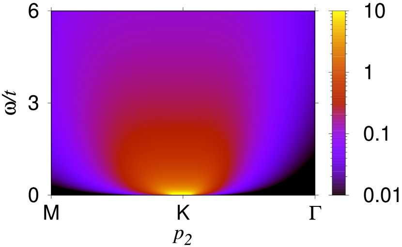
Figure 14: Spin spectral function $\chi^{\prime\prime}(\delta\boldsymbol{p}_{2},\omega)$ in Eq. (86) along the high-symmetry path $\boldsymbol{M}(\pi,0)\rightarrow\boldsymbol{K}(\pi,\pi)\rightarrow\boldsymbol{\Gamma}(0,0)$. Here, we have used the parameters $t=1$, $J_{\mathrm{K}}=2.5$, $J_{\mathrm{H}}=0.5$, $S=1/2$, $\tilde{c}_{B}=0.447$, and $\alpha=0.3$.

Appendix E Mean-field theory in paramagnetic phase

In this section, we study the structure of the mean-field theory in further detail, to provide some analytic understanding of the numerical observations made in Sec. II.2, in particular, the existence of two-dimensional states. We focus on the paramagnetic Kondo phase to simplify the procedure. Setting the magnetic order parameters $m_{c,f}$ and also $\lambda$ to zero, in order to ensure particle-hole symmetry, the mean-field Hamiltonian from Eq. (20) acquires the form

$$\hat{H}_{\text{MF}} =\!\!\!\!\sum_{\begin{subarray}{c}\boldsymbol{k}_{2},R_{z}\\ \sigma\end{subarray}}\!\!\!\left[\epsilon_{\boldsymbol{k}_{2}}c^{\dagger}_{\boldsymbol{k}_{2},R_{z},\sigma}c_{\boldsymbol{k}_{2},R_{z},\sigma}\!-\!t(c^{\dagger}_{\boldsymbol{k}_{2},R_{z}+1,\sigma}c_{\boldsymbol{k}_{2},R_{z},\sigma}\!+\!\text{h.c.})\!\right]$$

$$-J_{\mathrm{K}}V\sum_{\boldsymbol{k}_{2},\sigma}\left(\hat{c}_{\boldsymbol{k}_{2},R_{z}=0,\sigma}^{\dagger}\hat{f}_{\boldsymbol{k}_{2},\sigma}+\text{h.c.}\right)+L^{2}J_{\mathrm{K}}V^{2}\,.$$ (87)

Here, we have performed a partial Fourier transform to the in-plane momentum space, but kept the formulation of the out-of-plane dimension in real space, as in the main text. This brings the in-plane part of the tight-binding Hamiltonian to a diagonal form, as seen in the first line of the above equation. Solving the mean-field theory requires to diagonalize the given one-particle Hamiltonian. Physically, this is equivalent to finding the eigenstates of the Schrödinger equation $\hat{H}_{\text{MF}}|\psi\rangle=E|\psi\rangle$. For each $\boldsymbol{k}_{2}$, $\hat{H}_{\text{MF}}$ acts on a $L+1$ dimensional Hilbert-space formed by the chain of $L$ $c$ sites along the $z$ direction and the additional $f$ site. In the following, we label the $c$ sites as $R_{z}=-L/2,-L/2+1,...,0,...L/2-1$ for even $L$ with periodic boundary conditions and the $f$-site simply by $f$. Since only the site at $R_{z}=0$ is coupled to the additional $f$ orbital via the hybridization parameter $V$, the translational symmetry of the chain is broken in the presence of finite $V$. Consequently, the $L+1$-dimensional eigenvectors $(\psi(R_{z}),\psi(f))$ of $\hat{H}_{\text{MF}}$ are not given by Bloch states.

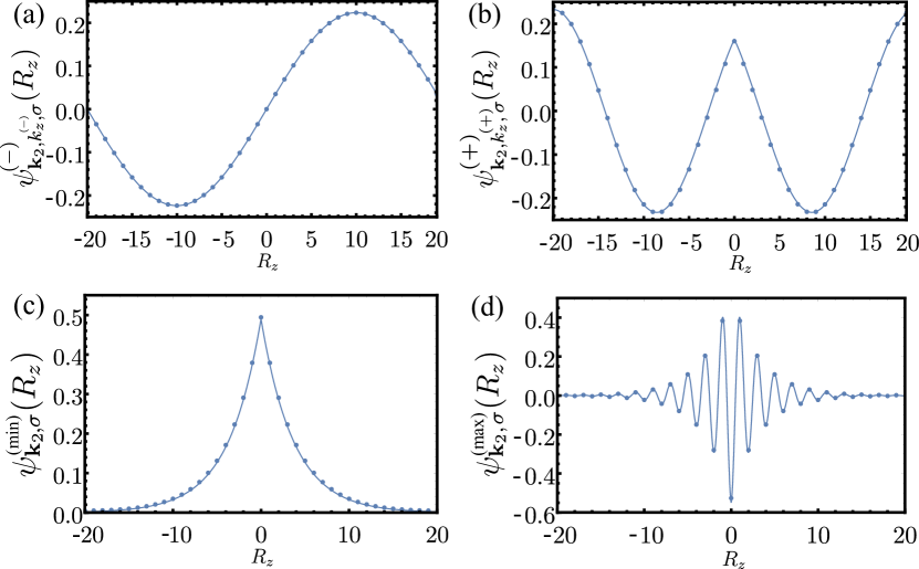
Figure 15: Examples of the different wave functions on the $c$ sites for system size $L=40$: The dots represent the eigenstates obtained by diagonalizing $\hat{H}_{\text{MF}}$ numerically at $J_{\mathrm{K}}/t=5.1$, $V/t=0.2$, and $\epsilon_{\boldsymbol{k}_{2}}/t=-0.2$. The solid lines are comparisons with the analytic solutions given in the text for this set of parameters. In particular, the extended states in the first line are (a) odd superpositions of Bloch waves and (b) even scattering states with phase shift. The second line shows the two-dimensional states with (c) minimal and (d) maximal energy.

There are three different types of wave functions:

Odd superpositions of Bloch waves of the unperturbed lattice at $\mathit{J_{K}=0}$.

These are characterized by the wave vectors $k^{(-)}_{z}$,

$$\begin{split}\psi^{(-)}_{\boldsymbol{k}_{2},k^{(-)}_{z},\sigma}(R_{z})&=\sqrt{\frac{2}{L}}\sin(k^{(-)}_{z}R_{z})\,,\\ \psi^{(-)}_{\boldsymbol{k}_{2},k^{(-)}_{z},\sigma}(f)&=0\,,\end{split}$$ (88)

associated with the noninteracting Bloch energies $E^{(-)}_{\boldsymbol{k}_{2},k^{(-)}_{z}}=\epsilon_{\boldsymbol{k}_{2}}+\epsilon_{k^{(-)}_{z}}$ from the tight-binding dispersion. The $k_{z}^{(-)}$ are given by the wave vectors of the free tight-binding chain $k_{z}=2\pi n/L,\;n\in\{-L/2,-L/2+2,\dots,L/2-1\}$ excluding $k_{z}=0$ and $k_{z}=\pi$, which give only rise to vanishing wave functions. This implies $L/2-1$ different eigenstates $\psi^{(-)}$. Physically, they are not affected by the interactions, because of the zero amplitude in the impurity layer, $\psi^{(-)}_{\boldsymbol{k}_{2},k_{z},\sigma}(R_{z}=0)=0$.

Even scattering states.

These are described by a wave vector $k_{z}^{(+)}$ and an associated phase shift $\phi_{k_{z}^{(+)}}$:

$$\begin{split}\psi^{(+)}_{\boldsymbol{k}_{2},k^{(+)}_{z},\sigma}(R_{z})&=A^{(+)}\sqrt{\frac{2}{L}}\cos\left(k_{z}^{(+)}R_{z}+\phi_{k_{z}^{(+)}}\operatorname{sgn}R_{z}\right),\\ \psi^{(+)}_{\boldsymbol{k}_{2},k^{(+)}_{z},\sigma}(f)&=A^{(+)}\sqrt{\frac{2}{L}}\frac{2\sin k^{(+)}_{z}\sin\phi_{k_{z}^{(+)}}}{J_{\mathrm{K}}V}\,,\end{split}$$ (89)

with energy $E^{(+)}_{\boldsymbol{k}_{2},k_{z}}=\epsilon_{\boldsymbol{k}_{2}}+\epsilon^{(+)}_{k_{z}}$ and amplitude $A^{(+)}$. Note that the wave functions are continuous at $R_{z}=0$, but the slopes differ when approaching $R_{z}=0$ from the left or the right. Periodicity restricts the wave vectors to the form

$$k_{z}^{(+)}=\frac{2\pi n-2\phi_{k_{z}^{(+)}}}{L}=\frac{k_{z}-2\phi_{k_{z}^{(+)}}}{L}\,,$$ (90)

while the phase shifts are obtained from the equation

$$\sin k_{z}^{(+)}\tan\phi_{k_{z}^{(+)}}=-\frac{J_{\mathrm{K}}^{2}V^{2}}{2(\epsilon_{\boldsymbol{k}_{2}}+\epsilon_{k^{(+)}_{z}})}\,.$$ (91)

Since the right-hand side is not bounded and may attain both positive and negative values, the phase shifts may vary in the interval $\phi_{k_{z}^{(+)}}\in[-\pi/2,\pi/2]$. According to Eq. (90), every $k^{(+)}_{z}$ is therefore adiabatically connected to the closest noninteracting wave vector $k_{z}$ since adjacent $k_{z}$ differ by $2\pi/L$. In total, there are $L/2$ different scattering states $\psi^{(+)}_{\boldsymbol{k}_{2},k^{(+)}_{z},\sigma}$.

Two two-dimensional states.

Neglecting corrections that are exponentially small in the system size, we have:

1. A state below the minimum of the tight-binding dispersion $\min_{k_{z}}(\epsilon_{\boldsymbol{k}_{2}}+\epsilon_{k_{z}})$:

   $$\begin{split}\psi^{(\min)}_{\boldsymbol{k}_{2},\sigma}(R_{z})&=A^{(\min)}e^{-\kappa|R_{z}|}\,,\quad\kappa>0\,,\\ \psi^{(\min)}_{\boldsymbol{k}_{2},\sigma}(f)&=A^{(\min)}\frac{2t\sinh\kappa}{J_{\mathrm{K}}V}\,,\end{split}$$ (92)

   with energy $E^{(\min)}_{\boldsymbol{k}_{2}}=\epsilon_{\boldsymbol{k}_{2}}-2t\cosh\kappa$. The parameter $\kappa$ satisfies

   $$\sinh\kappa=-\frac{J_{\mathrm{K}}^{2}V^{2}}{2t(\epsilon_{\boldsymbol{k}_{2}}-2t\cosh\kappa)}\,,$$ (93)

   and the normalization reads $A^{(\min)}=[1-2/(1-\exp(2\kappa))+(2t/J_{\mathrm{K}}V)^{2}\sinh^{2}\kappa]^{-1/2}$. Since $\cosh\kappa>1$ for all real $\kappa\neq 0$, this state has indeed an energy below the tight-binding energies of the extended states discussed before. By inserting $E^{(\min)}_{\boldsymbol{k}_{2}}$ into the right-hand-side of the last equation, we find furthermore $E^{(\min)}_{\boldsymbol{k}_{2}}<0$.

2. A state of maximal energy above $\max_{k_{z}}(\epsilon_{\boldsymbol{k}_{2}}+\epsilon_{k_{z}})$

   $$\begin{split}\psi^{(\max)}_{\boldsymbol{k}_{2},\sigma}(R_{z})&=A^{(\max)}\cos(\pi R_{z})e^{-\kappa|R_{z}|}\,,\quad\kappa>0\,,\\ \psi^{(\max)}_{\boldsymbol{k}_{2},\sigma}(f)&=-A^{(\max)}\frac{2t\sinh(\kappa)}{J_{\mathrm{K}}V}\,,\end{split}$$ (94)

   with energy $E^{(\max)}_{\boldsymbol{k}_{2}}=\epsilon_{\boldsymbol{k}_{2}}+2t\cosh\kappa$, where

   $$\sinh\kappa=\frac{J_{\mathrm{K}}^{2}V^{2}}{2t(\epsilon_{\boldsymbol{k}_{2}}+2t\cosh\kappa)}\,,$$ (95)

   and $A^{(\max)}=A^{(\min)}$. Here, we have in addition $E^{(\max)}_{\boldsymbol{k}_{2}}$.

The presence of two-dimensional states has already been anticipated in Sec. II.2: The spectral functions in Fig. 4 show sharp features of definite sign above and below the continuum of tight-binding energies. Note that these are observable irrespective of the presence of antiferromagnetic order.

In total, we find $(L/2-1)+L/2+2=L+1$ eigenstates, as expected for a Hamiltonian of dimension $(L+1)^{2}$. Plots of the different states can be found in Fig. 15.

After solving the effective Schrödinger equation, we can rewrite the mean-field Hamiltonian from Eq. (47) in diagonal form as follows

$$\begin{split}H_{\text{MF}}&=J_{\mathrm{K}}L^{2}V^{2}+\sum_{\boldsymbol{k}_{2},\sigma}\sum_{k_{z},s=\pm}E^{(s)}_{\boldsymbol{k}_{2},k^{(s)}_{z}}c^{\dagger}_{\boldsymbol{k}_{2},k^{(s)}_{z},\sigma}c_{\boldsymbol{k}_{2},k^{(s)}_{z},\sigma}\\ &\quad+\sum_{\boldsymbol{k}_{2},\sigma}\sum_{s=\min,\max}E^{(s)}_{\boldsymbol{k}_{2}}c^{\dagger}_{\boldsymbol{k}_{2},s,\sigma}c_{\boldsymbol{k}_{2},s,\sigma}\,.\end{split}$$ (96)

Here, the new fermionic operators $c_{\boldsymbol{k}_{2},k^{(\pm)}_{z},\sigma}$ annihilate a quasiparticle in the extended state $\psi^{(\pm)}_{\boldsymbol{k}_{2},k^{(\pm)}_{z},\sigma}$, whereas $c_{\boldsymbol{k}_{2},s,\sigma}$, with $s=\min,\max$, annihilates a fermion in the two-dimensional state $\psi^{(s)}_{\boldsymbol{k}_{2},s,\sigma}$, and analogously for the creation operators. Furthermore, the matrix elements required to transform the operators from the $(R_{z},f)$ basis to the new one are also given by the corresponding wave functions. In the ground state, the quasiparticles form, at the mean-field level, a Fermi sea with energy

$$E_{0}=J_{\mathrm{K}}L^{2}V^{2}+\!\sum_{\boldsymbol{k}_{2},\sigma}\!\frac{1}{2}\sum_{k^{(\pm)}_{z}}\theta(-E^{(\pm)}_{\boldsymbol{k}_{2},k^{(\pm)}_{z}})E^{(\pm)}_{\boldsymbol{k}_{2},k^{(\pm)}_{z}}+\!\sum_{\boldsymbol{k}_{2},\sigma}\!E^{(\min)}_{\boldsymbol{k}_{2}}\,.$$ (97)

The factor $1/2$ in the first sum is needed to avoid double counting of the extended states. The mean-field parameter $V$ satisfies the equation $\partial E_{0}/\partial V=0$. However, one may ask about the behavior of $V$ in the thermodynamic limit $L\to\infty$, since the contributions from the extended states in $E_{0}$ scale like the volume of the system $L^{3}$, whereas all other terms only scale like the area of the layer $L^{2}$. To answer this question, we first note that the energies $E^{(-)}$ drop out in $\partial E_{0}/\partial V$ because they are independent of $V$. To simplify the contribution from the extended scattering states with energies $E^{(+)}$, we use the adiabatic connection between them and the Bloch states. We can consider Eqs. (91) and (90) as an iterative scheme to determine both $k_{z}^{(+)}$ and $\phi_{k_{z}^{(+)}}$ at finite $J_{\mathrm{K}}$. Take as initial condition a Bloch state that is part of the noninteracting three-dimensional Fermi surface shown in Fig. 1(b) with momentum $(\boldsymbol{k}_{2},k_{z})$, with $k_{z}\neq 0,-\pi$, and eigenenergy $\epsilon_{\boldsymbol{k}_{2}}+\epsilon_{k_{z}}<0$. In this case, Eq. (91) generates a phase shift that obeys $\operatorname{sgn}\phi_{k^{(+)}_{z}}=\operatorname{sgn}k_{z}$. As a result, Eq. (90) implies $|k_{z}^{(+)}|<|k_{z}|$ and therefore $E^{(+)}_{\boldsymbol{k}_{2},k^{(+)}_{z}}<0$, such that the resulting scattering state at finite $J_{\mathrm{K}}$ is part of the Fermi sea of quasiparticles. On the contrary, initializing the procedure with a Bloch state with positive energy gives rise to an interacting state with $E^{(+)}_{\boldsymbol{k}_{2},k^{(+)}_{z}}>0$. Finally, Eqs. (91) and (90) imply that the values $k_{z}=0$ and $k_{z}=-\pi$ are mapped to $k^{(+)}_{z}=\mathcal{O}(L^{-1})$ and $k^{(+)}_{z}=-\pi+\mathcal{O}(L^{-1})$, respectively. Consequently, we have $\theta(-E^{(+)}_{\boldsymbol{k}_{2},k_{z}})=\theta(-\epsilon_{\boldsymbol{k}_{2}}-\epsilon_{k_{z}})$ in the limit $L\to\infty$ and, moreover,

$$\sum_{k^{(+)}_{z}}\theta(-E^{(+)}_{\boldsymbol{k}_{2},k^{(+)}_{z}})E^{(+)}_{\boldsymbol{k}_{2},k^{(+)}_{z}}=\\ \sum_{k_{z}}\theta(-\epsilon_{\boldsymbol{k}_{2}}-\epsilon_{k_{z}})\left(\epsilon_{\boldsymbol{k}_{2}}-\epsilon_{k_{z}}-\frac{2t}{L}\sin k_{z}\phi_{k^{(+)}_{z}}+\mathcal{O}(L^{-2})\right)\,.$$ (98)

With the above, the mean-field equation for $\partial E_{0}/\partial V=0$ becomes independent of system size in the thermodynamic limit,

$$J_{\mathrm{K}}V-t\!\!\int_{\text{3D FS}}\!\!\frac{d^{2}\boldsymbol{k}_{2}dk_{z}}{(2\pi)^{3}}\sin k_{z}\frac{\partial\phi_{k^{(+)}_{z}}}{\partial V}=2t\!\!\int\!\!\frac{d^{2}\boldsymbol{k}_{2}}{(2\pi)^{2}}\frac{\partial\cosh\kappa}{\partial V}\,.$$ (99)

The solution to the above equation corresponds to the behavior of $V$ in the paramagnetic heavy-fermion phase in Fig. 2. The asymptotics of $V$ in the limit $J_{\mathrm{K}}\to\infty$ can be extracted in closed form: Equation (91) entails that all phase shifts approach $\phi_{k^{(+)}_{z}}\to\pm\pi/2$, irrespective of $V$. Furthermore, from Eq. (93), we find $\cosh\kappa\approx J_{\mathrm{K}}|V|/(2t)$. Searching for a real, positive $V$, the solution approaches

$$J_{\mathrm{K}}V=2t\int\frac{d^{2}\boldsymbol{k}_{2}}{(2\pi)^{2}}\frac{J_{\mathrm{K}}}{2t}\quad\Rightarrow\quad V=1\,,$$ (100)

which agrees with the numerical evaluation presented in Sec. II.2. Furthermore, we can answer how many quasiparticle states are occupied at a given in-plane momentum $\boldsymbol{k}_{2}$. As discussed above, the Bloch eigenstates of $\hat{H}_{\mathrm{Fermi}}$ with wave vector $(\boldsymbol{k}_{2},k_{z})$ are mapped to the eigenstates of $\hat{H}_{\text{MF}}$ as follows: $k_{z}=0,-\pi$ have corresponding extended scattering states (b) whereas all other pairs $\pm k_{z}$ form one odd state of type (a) and one even state of type (b). Since $\operatorname{sgn}E^{(\pm)}_{\boldsymbol{k}_{2},k_{z}^{(\pm)}}=\operatorname{sgn}(\epsilon_{\boldsymbol{k}_{2}}+\epsilon_{k_{z}})$ we have one quasiparticle for every occupied Bloch state of the noninteracting $3d$ FS. In addition, the two-dimensional state (c1) with minimal, negative energy is also occupied. The number of quasiparticles with $\boldsymbol{k}_{2}$ is thus $\langle\hat{n}_{c}(\boldsymbol{k}_{2})\rangle+1$. As discussed in the main text, we therefore have $L+1$ electrons per lattice site and the $f$ fermion participates indeed in the Luttinger count.

Finally, we consider the structure of the resulting propagators. The effects of interactions at the mean-field level are most easily determined by representing the hybridization part of $\hat{H}_{\text{MF}}$ from Eq. (E) completely in momentum space. This yields the term $-J_{\mathrm{K}}VL^{-1/2}\sum_{\boldsymbol{k}_{2},k_{z},\sigma}\left(\hat{c}_{\boldsymbol{k}_{2},k_{z},\sigma}^{\dagger}\hat{f}_{\boldsymbol{k}_{2},\sigma}+\text{h.c.}\right)\,$. Firstly, this implies the self-energy of the conduction electrons

$$\Sigma^{\text{MF}}_{c}(\omega,\boldsymbol{k}_{2})_{k_{z},k^{\prime}_{z}}=\frac{J_{\mathrm{K}}^{2}V^{2}}{L}G^{(0)}_{f}(\omega,\boldsymbol{k}_{2})=\frac{J_{\mathrm{K}}^{2}V^{2}}{L}\frac{1}{i\omega}\,,$$ (101)

which is off-diagonal in the out-of-plane direction because one-dimensional scattering events break the conservation of momentum. Secondly, the self-energy in the $f$ sector is given by

$$\Sigma^{\text{MF}}_{f}(\omega,\boldsymbol{k}_{2})=J_{\mathrm{K}}^{2}V^{2}g_{0}(\omega,\boldsymbol{k}_{2})\,.$$ (102)

The solution of the Dyson equation for the conduction electrons is therefore obtained by dressing the propagator by the scattering $T$ matrix of the (dynamical) potential,

$$G_{c,\sigma}^{\text{MF}}(\boldsymbol{k}_{2},\omega)_{k_{z},k^{\prime}_{z}}=G_{c,\sigma}^{(0)}(\boldsymbol{k}_{2},\omega,k_{z})\delta_{k_{z},k^{\prime}_{z}}\\ +G_{\sigma}^{(0)}(\omega,\boldsymbol{k}_{2},k_{z})T^{\text{MF}}(\boldsymbol{k}_{2},\omega)G_{c,\sigma}^{(0)}(\boldsymbol{k}_{2},\omega,k^{\prime}_{z})\,,$$ (103)

with the $T$ matrix

$$\begin{split}T^{\text{MF}}(\boldsymbol{k}_{2},\omega)_{k_{z},k^{\prime}_{z}}=\frac{\Sigma_{c}^{\text{MF}}(\omega,\boldsymbol{k}_{2})_{k_{z},k^{\prime}_{z}}}{1-\Sigma_{c}^{\text{MF}}(\omega,\boldsymbol{k}_{2})_{k_{z},k^{\prime}_{z}}g_{0}(\boldsymbol{k}_{2},\omega)}\,.\end{split}$$ (104)

We note that Eqs. (103) and (104) correspond to Eqs. (48) and (49), but here in the case of a single band due to the absence of sublattice magnetization. The propagator of the $f$ electrons reads in turn

$$G^{\text{MF}}_{f}=\frac{1}{i\omega-\Sigma^{\text{MF}}_{f}(\omega,\boldsymbol{k}_{2})}=\frac{T^{\text{MF}}(\boldsymbol{k}_{2},\omega,R_{z}=0)}{J_{\mathrm{K}}^{2}V^{2}}\,,$$ (105)

which give rise to the local spectral function in Eq. (23). After analytic continuation to real frequencies, the two-dimensional-states manifest themselves via poles in the spectral functions $A_{c,f}(\omega,\boldsymbol{k}_{2})$ at energies $\omega=\epsilon_{\boldsymbol{k}_{2}}\pm 2t\cosh\kappa$. As discussed in the main text, the $\boldsymbol{k}_{2}$-integrated spectral functions show therefore logarithmic van-Hove singularities that are typical for two-dimensional systems.

References

- v. Löhneysen et al. [2007] H. v. Löhneysen, A. Rosch, M. Vojta, and P. Wölfle, Fermi-liquid instabilities at magnetic quantum phase transitions, Rev. of Mod. Phys. 79, 1015 (2007).
- Coleman [2007] P. Coleman, in Handbook of Magnetism and Advanced Magnetic Materials, Vol. 1 (Wiley, New York, 2007) pp. 95–148.
- Tsunetsugu et al. [1997] H. Tsunetsugu, M. Sigrist, and K. Ueda, The ground-state phase diagram of the one-dimensional Kondo lattice model, Rev. Mod. Phys. 69, 809 (1997).
- Lee et al. [2006] P. A. Lee, N. Nagaosa, and X.-G. Wen, Doping a Mott insulator: Physics of high-temperature superconductivity, Rev. Mod. Phys. 78, 17 (2006).
- Emery [1987] V. J. Emery, Theory of high- superconductivity in oxides, Phys. Rev. Lett. 58, 2794 (1987).
- Zhang and Rice [1988] F. C. Zhang and T. M. Rice, Effective Hamiltonian for the superconducting Cu oxides, Phys. Rev. B 37, 3759 (1988).
- Toskovic et al. [2016] R. Toskovic, R. van den Berg, A. Spinelli, I. S. Eliens, B. van den Toorn, B. Bryant, J. S. Caux, and A. F. Otte, Atomic spin-chain realization of a model for quantum criticality, Nat. Phys. 12, 656 (2016).
- Danu et al. [2021] B. Danu, Z. Liu, F. F. Assaad, and M. Raczkowski, Zooming in on heavy fermions in Kondo lattice models, Phys. Rev. B 104, 155128 (2021).
- Raczkowski et al. [2022] M. Raczkowski, B. Danu, and F. F. Assaad, Breakdown of heavy quasiparticles in a honeycomb Kondo lattice: A quantum Monte Carlo study, Phys. Rev. B 106, L161115 (2022).
- Danu et al. [2020] B. Danu, M. Vojta, F. F. Assaad, and T. Grover, Kondo Breakdown in a Spin- Chain of Adatoms on a Dirac Semimetal, Phys. Rev. Lett. 125, 206602 (2020).
- Danu et al. [2022] B. Danu, M. Vojta, T. Grover, and F. F. Assaad, Spin chain on a metallic surface: Dissipation-induced order versus Kondo entanglement, Phys. Rev. B 106, L161103 (2022).
- Shishido et al. [2010] H. Shishido, T. Shibauchi, K. Yasu, T. Kato, H. Kontani, T. Terashima, and Y. Matsuda, Tuning the Dimensionality of the Heavy Fermion Compound CeIn3, Science 327, 980 (2010).
- Hirsch [1985] J. E. Hirsch, Two-dimensional Hubbard model: Numerical simulation study, Phys. Rev. B 31, 4403 (1985).
- Wu and Zhang [2005] C. Wu and S.-C. Zhang, Sufficient condition for absence of the sign problem in the fermionic quantum Monte Carlo algorithm, Phys. Rev. B 71, 155115 (2005).
- Li et al. [2016] Z.-X. Li, Y.-F. Jiang, and H. Yao, Majorana-Time-Reversal Symmetries: A Fundamental Principle for Sign-Problem-Free Quantum Monte Carlo Simulations, Phys. Rev. Lett. 117, 267002 (2016).
- Haldane [1988] F. D. M. Haldane, O(3) Nonlinear Model and the Topological Distinction between Integer- and Half-Integer-Spin Antiferromagnets in Two Dimensions, Phys. Rev. Lett. 61, 1029 (1988).
- Zhang and Yu [2000] G.-M. Zhang and L. Yu, Kondo singlet state coexisting with antiferromagnetic long-range order: A possible ground state for Kondo insulators, Phys. Rev. B 62, 76 (2000).
- Raczkowski and Assaad [2020] M. Raczkowski and F. F. Assaad, Phase diagram and dynamics of the symmetric Kondo lattice model, Phys. Rev. Research 2, 013276 (2020).
- Costi [2000] T. A. Costi, Kondo Effect in a Magnetic Field and the Magnetoresistivity of Kondo Alloys, Phys. Rev. Lett. 85, 1504 (2000).
- Borda et al. [2007] L. Borda, L. Fritz, N. Andrei, and G. Zaránd, Theory of inelastic scattering from quantum impurities, Phys. Rev. B 75, 235112 (2007).
- Maltseva et al. [2009] M. Maltseva, M. Dzero, and P. Coleman, Electron Cotunneling into a Kondo Lattice, Phys. Rev. Lett. 103, 206402 (2009).
- Raczkowski and Assaad [2019] M. Raczkowski and F. F. Assaad, Emergent Coherent Lattice Behavior in Kondo Nanosystems, Phys. Rev. Lett. 122, 097203 (2019).
- Schrieffer and Wolff [1966] J. R. Schrieffer and P. A. Wolff, Relation between the Anderson and Kondo Hamiltonians, Phys. Rev. 149, 491 (1966).
- Assaad et al. [2022] F. F. Assaad, M. Bercx, F. Goth, A. Götz, J. S. Hofmann, E. Huffman, Z. Liu, F. P. Toldin, J. S. E. Portela, and J. Schwab, The ALF (Algorithms for Lattice Fermions) project release 2.0. Documentation for the auxiliary-field quantum Monte Carlo code, SciPost Phys. Codebases 1 (2022).
- Assaad and Evertz [2008] F. Assaad and H. Evertz, in Computational Many-Particle Physics, Lecture Notes in Physics, Vol. 739, edited by H. Fehske, R. Schneider, and A. Weiße (Springer, Berlin Heidelberg, 2008) pp. 277–356.
- Blankenbecler et al. [1981] R. Blankenbecler, D. J. Scalapino, and R. L. Sugar, Monte Carlo calculations of coupled boson-fermion systems. I, Phys. Rev. D 24, 2278 (1981).
- White et al. [1989] S. White, D. Scalapino, R. Sugar, E. Loh, J. Gubernatis, and R. Scalettar, Numerical study of the two-dimensional Hubbard model, Phys. Rev. B 40, 506 (1989).
- Sugiyama and Koonin [1986] G. Sugiyama and S. Koonin, Auxiliary field Monte-Carlo for quantum many-body ground states, Ann. Phys. 168, 1 (1986).
- Sorella et al. [1989] S. Sorella, S. Baroni, R. Car, and M. Parrinello, A Novel Technique for the Simulation of Interacting Fermion Systems, Europhys. Lett. 8, 663 (1989).
- Assaad [2002] F. F. Assaad, Depleted Kondo lattices: Quantum Monte Carlo and mean-field calculations, Phys. Rev. B 65, 115104 (2002).
- Gross [1992] C. Gross, The boundary condition integration technique: Results for the Hubbard model in 1d and 2d, Z. Phys. B 86, 359 (1992).
- Sandvik [1998] A. Sandvik, Stochastic method for analytic continuation of quantum Monte Carlo data, Phys. Rev. B 57, 10287 (1998).
- Beach [2004] K. S. D. Beach, Identifying the maximum entropy method as a special limit of stochastic analytic continuation, arXiv:cond-mat/0403055 .
- Capponi and Assaad [2001] S. Capponi and F. F. Assaad, Spin and charge dynamics of the ferromagnetic and antiferromagnetic two-dimensional half-filled Kondo lattice model, Phys. Rev. B 63, 155114 (2001).
- Vojta [2010] M. Vojta, Orbital-Selective Mott Transitions: Heavy Fermions and Beyond, J. Low Temp. Phys. 161, 203 (2010).
- Vojta [2008] M. Vojta, From itinerant to local-moment antiferromagnetism in Kondo lattices: Adiabatic continuity versus quantum phase transitions, Phys. Rev. B 78, 125109 (2008).
- Hertz [1976] J. A. Hertz, Quantum critical phenomena, Phys. Rev. B 14, 1165 (1976).
- Millis [1993] A. J. Millis, Effect of a nonzero temperature on quantum critical points in itinerant fermion systems, Phys. Rev. B 48, 7183 (1993).
- Weber et al. [2022] M. Weber, D. J. Luitz, and F. F. Assaad, Dissipation-Induced Order: The Quantum Spin Chain Coupled to an Ohmic Bath, Phys. Rev. Lett. 129, 056402 (2022).
- Byers and Yang [1961] N. Byers and C. N. Yang, Theoretical Considerations Concerning Quantized Magnetic Flux in Superconducting Cylinders, Phys. Rev. Lett. 7, 46 (1961).
- Altland and Simons [2010] A. Altland and B. D. Simons, Condensed Matter Field Theory, 2nd ed. (Cambridge University Press, Cambridge, 2010).