The Projected Covariance Measure for assumption-lean variable significance testing

Abstract

Testing the significance of a variable or group of variables $X$ for predicting a response $Y$, given additional covariates $Z$, is a ubiquitous task in statistics. A simple but common approach is to specify a linear model, and then test whether the regression coefficient for $X$ is non-zero. However, when the model is misspecified, the test may have poor power, for example when $X$ is involved in complex interactions, or lead to many false rejections. In this work we study the problem of testing the model-free null of conditional mean independence, i.e. that the conditional mean of $Y$ given $X$ and $Z$ does not depend on $X$. We propose a simple and general framework that can leverage flexible nonparametric or machine learning methods, such as additive models or random forests, to yield both robust error control and high power. The procedure involves using these methods to perform regressions, first to estimate a form of projection of $Y$ on $X$ and $Z$ using one half of the data, and then to estimate the expected conditional covariance between this projection and $Y$ on the remaining half of the data. While the approach is general, we show that a version of our procedure using spline regression achieves what we show is the minimax optimal rate in this nonparametric testing problem. Numerical experiments demonstrate the effectiveness of our approach both in terms of maintaining Type I error control, and power, compared to several existing approaches.

1 Introduction

Understanding the relationship between a response and associated predictors is one of the most common problems faced by data analysts across many diverse areas of science and industry. Often an important step in this task is to determine which variables or groups of variables are important in this relationship. To fix ideas, consider data formed of independent copies of a triple $(X,Y,Z)$, where $Y\in{\mathbb{R}}$ is our response, and we wish to assess the significance of a group of predictors $X\in{\mathbb{R}}^{d_{X}}$ after adjusting for confounding variables $Z\in{\mathbb{R}}^{d_{Z}}$; we will consider a more general setting later in this paper where $X$ and $Z$ can be potentially non-Euclidean. One simple but popular way of addressing this problem is to fit a linear regression model $Y=X^{\top}\beta+Z^{\top}\gamma+\varepsilon$, where we assume that the random error $\varepsilon$ satisfies ${\mathbb{E}}(\varepsilon\,|\,X,Z)=0$, and perform an $F$-test for the significance of $X$ (i.e. test the null hypothesis that $\beta=0$). However, in the case that the linear model is not a sufficiently good approximation of the ground truth, this can result in wrongly declaring $X$ to be important or unimportant, and other significance tests based on parametric models suffer from similar issues. The fact that regressions based on parametric models are typically greatly outperformed by modern machine learning methods such as deep learning (Goodfellow et al.,, 2016) and random forests (Breiman,, 2001) in regression competitions such as those hosted by Kaggle (Bojer and Meldgaard,, 2021), suggests that such parametric models giving poor approximations to the truth is the norm rather than the exception, at least in contemporary datasets of interest.

In this work we consider the model-free null hypothesis of conditional mean independence, that is ${\mathbb{E}}(Y\,|\,X,Z)={\mathbb{E}}(Y\,|\,Z)$; in words, $X$ does not feature in the regression function of $Y$ on $X$ and $Z$. It is interesting to compare this to the conditional independence null $Y\mbox{${}\perp\mkern-11.0mu\perp{}$}X\,|\,Z$, which has attracted much attention in recent years. The latter asks not just for the regression function to be expressed as a function of $Z$ alone, but in fact for the entire conditional distribution of $Y$ given $(X,Z)$ to equal the conditional distribution of $Y$ given $Z$. Any valid test of conditional mean independence may be used as a test for conditional independence as its size is no larger than its size over the larger null hypothesis of conditional mean independence. The two nulls in fact coincide when $Y$ is binary, but more generally there are important differences. One attractive property of the conditional mean independence null is that the alternative of conditional mean dependence may be characterised by the property that $X$ can improve the prediction of $Y$ in a mean-squared error sense, given knowledge of $Z$. For example, consider the setting where $X$ is a binary treatment variable, $Z$ contains all pre-treatment confounders and $Y$ is the observed outcome. Under assumptions (including the absence of unmeasured confounders) that are standard in the causal inference literature (Neyman,, 1923; Rubin,, 1974), conditional mean dependence is equivalent to the existence of a subgroup average treatment effect, that is a (measurable) subset $\mathcal{A}\subseteq{\mathbb{R}}^{d_{Z}}$ where ${\mathbb{E}}\{{\mathbb{E}}(Y\,|\,Z,X=1)\,|\,Z\in\mathcal{A}\}>{\mathbb{E}}\{{\mathbb{E}}(Y\,|\,Z,X=0)\,|\,Z\in\mathcal{A}\}$. On the other hand, rejection of the conditional independence null does not in general have an immediate interpretation in terms of its predictive implications.

Despite the attractions of conditional mean independence, an important issue is that this property is not testable without further restrictions on the null hypothesis: if $(X,Y,Z)$ have a density that is absolutely continuous with respect to Lebesgue measure, then the power of any test at any alternative is at most its size. This comes as a direct consequence of the untestability of the smaller conditional independence null (Shah and Peters,, 2020). The conclusion is that in order to test conditional mean independence, one must further constrain the null hypothesis in some way.

Given the success of machine learning methods in prediction problems, a natural and convenient way to specify these constraints is based on restricting the set of nulls to those where user-chosen regression methods can estimate certain conditional expectations sufficiently well. One strategy, as adopted in the Generalised Covariance Measure (GCM) of Shah and Peters, (2020), involves, in the case where $X$ is univariate, regressing each of $X$ and $Y$ on $Z$, computing the covariance between the resulting residuals and estimating a normalised version of ${\mathbb{E}}\{{\mathrm{Cov}}(X,Y\,|\,Z)\}$, a quantity that is zero under conditional independence. A drawback of this approach, however, is that it has no power against alternatives to conditional mean independence where ${\mathbb{E}}\{{\mathrm{Cov}}(X,Y\,|\,Z)\}=0$.

To gain greater power, Shah and Peters, (2020) suggest to apply the above with $X$ replaced by each component of $\bigl{(}\phi_{1}(X,Z),\ldots,\phi_{m}(X,Z)\bigr{)}$, where $\phi_{1},\ldots,\phi_{m}:{\mathbb{R}}^{d_{X}\times d_{Z}}\to{\mathbb{R}}$ are a fixed user-chosen collection of transformations of the data. One may then base a final test on the maximum absolute value of the resulting test statistics. It is however not clear how one should choose these transformations, and if $m$ is large, or indeed $d_{X}$ is large and we use the strategy above but with the $\phi_{j}$ simply extracting the $j$th component of $X$, then performing all the regressions involved may be impractical. A related approach to improve the power properties of the GCM is introduced by Scheidegger et al., (2022), who propose a carefully-weighted version of the GCM that, under conditions, can have power against alternatives where we do not have ${\mathrm{Cov}}(X,Y\,|\,Z)=0$ almost surely; see also Fernández and Rivera, (2022). Nevertheless, it is perfectly possible to have ${\mathrm{Cov}}(X,Y\,|\,Z)=0$ under conditional mean dependence, and here even the weighted GCM would be powerless: for example, consider the simple setting where $(X,Z,\varepsilon)\sim N_{3}(0,\boldsymbol{I})$ and $Y=X^{2}+\varepsilon$. In this case, ${\mathrm{Cov}}(X,Y\,|\,Z)={\mathrm{Cov}}(X,Y)=0$ despite $X$ clearly being important for the prediction of $Y$. It is therefore of great interest to develop methods for testing conditional mean independence whose validity, as in the case of the GCM and its weighted version, relies primarily on the predictive properties of user-chosen regression methods, but which have power against much wider classes of alternatives.

While there has a great deal of research effort on the problem of conditional independence testing in recent years (we review the contributions most relevant to our work here in Section 1.2), there has been comparatively little on testing conditional mean independence. One compelling approach is based on an equivalent way of stating the null hypothesis: defining

$$\tau :={\mathbb{E}}\bigl{[}\bigl{\{}{\mathbb{E}}(Y\,|\,X,Z)-{\mathbb{E}}(Y\,|\,Z)\bigr{\}}^{2}\bigr{]}$$ (1)

we have that $\tau=0$ if and only if $Y$ is conditionally mean independent of $X$ given $Z$. This suggests a potential strategy for assessing conditional mean independence via the estimation of $\tau$. Such an approach was adopted by Williamson et al., (2021), who employed a plug-in estimator of $\tau$, and showed that, under conditions, it yields a semiparametric efficient estimator, provided that $\tau>0$. However, as highlighted by Williamson et al., (2021), under the null where $\tau=0$, semiparametric approaches such as this face a fundamental difficulty as the influence function is identically zero, and as a consequence the test statistic has a degenerate distribution.

To circumvent this issue, Williamson et al., (2022) and independently Dai et al., (2022), utilise an alternative representation of the target parameter $\tau={\mathbb{E}}[\{Y-{\mathbb{E}}(Y\,|\,Z)\}^{2}]-{\mathbb{E}}[\{Y-{\mathbb{E}}(Y\,|\,X,Z)\}^{2}]$ and propose a testing procedure via sample splitting, where estimation of ${\mathbb{E}}[\{Y-{\mathbb{E}}(Y\,|\,Z)\}^{2}]$ and ${\mathbb{E}}[\{Y-{\mathbb{E}}(Y\,|\,X,Z)\}^{2}]$ is done on independent splits of the data. This restores the asymptotic normality of the test statistic under the null, but estimating these population quantities separately comes with a significant power loss. Indeed, even in simple parametric settings, each of the population level quantities ${\mathbb{E}}[\{Y-{\mathbb{E}}(Y\,|\,Z)\}^{2}]$ and ${\mathbb{E}}[\{Y-{\mathbb{E}}(Y\,|\,X,Z)\}^{2}]$ can only be estimated at a $1/\sqrt{n}$ rate, and so the difference of the two estimates each coming from independent samples would also only converge to the true difference $\tau$ at a $1/\sqrt{n}$ rate. As a result, the test becomes asymptotically powerless if $\sqrt{n}\tau\rightarrow 0$, even for a parametric linear model where the optimal testing rate is known to be of order $n^{-1}$. Moreover, the asymptotic normality fails when $Y$ is (close to) independent of $(X,Z)$, which raises concerns about uniform validity of the test. See Sections S3 of the supplementary material for details on these issues.

1.1 Outline of our approach and contributions

In view of the considerations above, the goal of this paper is to propose a new framework for testing conditional mean independence that has the following properties:

• Flexible Type I error control. The user should be able to leverage flexible regression methods to ensure validity of the test uniformly over classes of distributions where these methods perform sufficiently well.

• Rate-optimal power in diverse settings. The test should have minimax rate-optimal power in both simple parametric models, as well as challenging nonparametric settings, when used with appropriate regression methods.

• Computationally practical. The test should involve performing only a small number of regressions.

Our approach is based on the following alternative characterisation of conditional mean independence: $Y$ is conditionally mean independent of $X$ given $Z$ if and only if

$${\mathbb{E}}\bigl{[}\bigl{\{}Y-{\mathbb{E}}(Y\,|\,Z)\bigr{\}}f(X,Z)\bigr{]}={\mathbb{E}}\bigl{[}{\mathrm{Cov}}\bigl{(}Y,f(X,Z)\,|\,Z\bigr{)}\bigr{]}=0$$ (2)

for all functions $f$ such that ${\mathbb{E}}\bigl{(}f(X,Z)^{2}\bigr{)}<\infty$. In words, the residuals $Y-{\mathbb{E}}(Y\,|\,Z)$ from regressing $Y$ on $Z$ alone are uncorrelated with any square-integrable function of $X$ and $Z$. On the other hand, under an alternative, these residuals should not be pure noise but contain some ‘signal’ that can be exposed via an appropriate $f$ such that the left-hand side of (2) is strictly positive.

To motivate our specific strategy, consider an oracular test statistic that uses knowledge of the conditional expectation ${\mathbb{E}}(Y\,|\,Z)$: given independent copies $(X_{i},Y_{i},Z_{i})_{i=1}^{n}$ of $(X,Y,Z)$ and a function $f$, the random variables $L_{i}^{*}:=\{Y_{i}-{\mathbb{E}}(Y_{i}\,|\,Z_{i})\}f(X_{i},Z_{i})$ for $i=1,\ldots,n$ are independent and identically distributed, with zero mean under the null. Writing $\widetilde{L}_{i}^{*}:=\{Y_{i}-{\mathbb{E}}(Y_{i}\,|\,X_{i},Z_{i})\}f(X_{i},Z_{i})$, we have that under regularity conditions, the studentised statistic

$$T^{*}:=\frac{\frac{1}{\sqrt{n}}\sum_{i=1}^{n}L_{i}^{*}}{\sqrt{\frac{1}{n}\sum_{i=1}^{n}\widetilde{L}_{i}^{*2}}}$$ (3)

converges to a standard normal distribution under the null, and may thus form the basis of a test. Note that since $\widetilde{L}_{i}^{*}=L_{i}^{*}$ under the null, we may alternatively studentise the test statistic using the empirical standard deviation of the $L_{i}^{*}$; however this version simplifies the derivation to follow.

Different choices of $f$ would lead to different power properties under an alternative. Ideally, we want to maximise the value of the test statistic under an alternative, so we would like ${\mathbb{E}}(L^{*}_{i})/\sqrt{{\mathrm{Var}}(\widetilde{L}_{i}^{*})}$ to be as large as possible. It may be shown (see Proposition S11 in Section S2.2 of the supplementary material) that this is uniquely maximised, up to an arbitrary positive scaling, by choosing $f(X,Z)=h(X,Z)/v(X,Z)$, where $h(X,Z):={\mathbb{E}}(Y\,|\,X,Z)-{\mathbb{E}}(Y\,|\,Z)$ and $v(X,Z):={\mathrm{Var}}(Y\,|\,X,Z)$. We therefore see that the optimal $f$ is a version of the projection $h$ of $Y$ onto the space of square-integrable functions of $(X,Z)$ that are orthogonal to functions of $Z$, inversely weighted by the conditional variance $v$.

The considerations above suggest the following approach: use one portion of the data to obtain an estimate $\widehat{f}$ of the projection $f$, and then use the remaining data to evaluate a test statistic of the form (3), with the unknown conditional expectations there replaced with appropriate regression estimates. This forms the basis of our proposed test statistic, which we call the Projected Covariance Measure (PCM). In fact, it turns out to be advantageous to modify somewhat the basic blueprint described above, for instance by subtracting from $\widehat{f}(X,Z)$ an estimate of its conditional expectation given $Z$, to reduce bias; a complete description of our methodology is given in Section 2.

One important issue to be addressed is the fact that under the null, $h$ is the zero function, and as a consequence, both the numerator and denominator of $T^{*}$ are zero. This is not immediately problematic for the oracular statistic $T^{*}$, as one can always decide not to reject the null when the numerator is precisely $0$. However, it might appear to be potentially disastrous for an empirical version of $T^{*}$, where any bias terms in the numerator could be inflated by division with a denominator that is close to zero. One of our main contributions in this work is to show that by formulating our PCM test statistic appropriately, it has an asymptotic standard Gaussian limit in settings ranging from low- and high-dimensional linear models to fully nonparametric settings. Moreover, we demonstrate empirically that this limiting behaviour can be expected to hold more generally when machine learning methods such as random forests (Breiman,, 2001) are used for the regressions involved.

The rest of the paper is organised as follows. After reviewing some related literature in Section 1.2, we present a full description of our PCM methodology in Section 2. In Section 3, we examine the simplest instantiation of our general framework and study testing in the context of low-dimensional linear models. An important revelation of this analysis is that in contrast to the equally general testing frameworks of Williamson et al., (2022) and Dai et al., (2022), our approach has power against local alternatives where $\tau$ is of order $n^{-1}$. We go on to show that, under conditions, the PCM maintains Type I error control in high-dimensional linear models, even when using an essentially arbitrary machine learning method to estimate the projection $f$. We present a general theory of the PCM in Section 4, giving conditions involving prediction errors of the user-chosen regression procedures used in the PCM that result in Type I error control, and also study the power of the procedure. In Section 5, we show how our general conditions for Type I error control may be satisfied in a fully nonparametric regression setting when using series estimators for the relevant regressions. We also introduce a slight variant of our approach involving additional sample splitting that enjoys what we show to be minimax rate optimal power over classes of alternatives for which $\tau$ in (1) satisfies a lower bound.

In Section 6, we conduct several simulation experiments that demonstrate the effectiveness of the PCM when used with generalised additive model-based regressions (Wood,, 2017) and random forests, in terms of both Type I error control and power. We conclude with a discussion in Section 7 outlining potential future research directions suggested by our work.

In Sections S1 and S2 of the supplementary material, we include the proofs of all our main results and related auxiliary lemmas. Section S4 provides a self-contained description of spline regression and related results that we use for our analysis in Section 5. In Section S5, we give a more detailed analysis of our results for linear projections in Section 3; in particular we derive an exact asymptotic power function of our test. Section S6 contains the results from additional numerical experiments beyond those included in Section 6.

1.2 Literature review

There is a relatively small body of literature that is explicitly concerned with conditional mean independence. Early developments on this topic include the work of Fan and Li, (1996), Lavergne and Vuong, (2000) and Aït-Sahalia et al., (2001) from the econometrics community. Jin et al., (2018) propose an approach for testing conditional mean independence in cases where $\mathbb{E}(Y\,|\,Z)$ is a linear function of $Z$, based on the martingale difference divergence proposed by Shao and Zhang, (2014).

Recent years have witnessed an increasing use of machine learning (ML) tools for statistical inference. For example, Chernozhukov et al., (2018) introduce an ML-driven approach for estimating causal parameters in the presence of complex nuisance parameters. Shah and Bühlmann, (2018) and Janková et al., (2020) propose methods for goodness-of-fit testing in high-dimensional (generalised) linear models that involve detecting remaining signal in residuals using ML methods. More closely related to this work, Williamson et al., (2022), and Dai et al., (2022), propose model-free methods for assessing conditional mean independence that can take advantage of existing ML algorithms. Williamson et al., (2022) derive a semiparametrically efficient estimator $\tau$, but recognise the difficulty of testing the null hypothesis that $\tau=0$ caused by the fact that the efficient influence function is identically zero under the null. This means that their sample-splitting approach lacks validity when $(X,Y,Z)$ are independent, and moreover it turns out that the test may require larger values of $\tau$ than necessary in order to achieve power; see Section 3.1 for a more detailed discussion. Dai et al., (2022) alleviate the Type I error issue by adding noise to their test statistic, but this comes at a further price in terms of power, as pointed out by Verdinelli and Wasserman, (2021). Cai et al., (2022) also propose model-free tests of conditional mean independence; one of their test statistics has a similar form to the one in Williamson et al., (2021) that compares the predictive performance of two regression models, and they use a permutation approach to calculate a $p$-value. Another related work is that of Zhang and Janson, (2020), who provide a method for constructing confidence intervals for $\tau$ in the case where the conditional distribution of $X$ given $Z$ is (almost) known; see also Candès et al., (2018) and Berrett et al., (2020), who employ similar assumptions in the context of testing conditional independence.

Many existing tests, including ours, determine their critical values based on asymptotic theory derived under the null. However, most work (implicitly) targets pointwise Type I error control that holds only each fixed null. This type of pointwise analysis leaves room for the existence of a sequence of null distributions for which the Type I error can be made arbitrarily large. A classical example is the fact that the $t$-test that has pointwise asymptotic size $\alpha$ for the class of distributions with finite variance, has uniform asymptotic size 1 for the same class of distributions (Romano,, 2004). While it is straightforward to introduce, for instance, moment conditions to restore uniform size control in that problem, we argue that the issue is even more pertinent in the context of testing conditional (mean) independence as there are no canonical choices of restrictions to the null that can yield this form of error control. In this work, we therefore put great emphasis on uniform Type I error control over classes of distributions in order to present more practically-relevant error guarantees. This uniform analysis is in line with recent work on conditional independence testing such as Shah and Peters, (2020), Petersen and Hansen, (2021), Lundborg et al., (2022), Scheidegger et al., (2022) and Neykov et al., (2021).

Our work builds on a classical technique, namely sample splitting, that involves partitioning the data into disjoint subsamples for different purposes: roughly speaking, a portion of the data is used for seeking a good direction that potentially contains a high signal and the other portion is used for conducting a test based on the data projected along the given direction. Cox, (1975) is one of the earliest papers that applies sample splitting to testing problems. Since then, many inference procedures have been developed by leveraging a similar technique to perform variable selection in high-dimensional models (Wasserman and Roeder,, 2009; Meinshausen et al.,, 2009; Meinshausen and Bühlmann,, 2010; Shah and Samworth,, 2013), inference after model selection (Rinaldo et al.,, 2019), changepoint detection (Wang and Samworth,, 2018) and inference based on maximum likelihood estimators (Wasserman et al.,, 2020), to name just a few. In a similar vein, Kim and Ramdas, (2023) introduce splitting-based procedures that address an issue of degenerate $U$-statistics for high-dimensional inference. While our main focus is on testing, sample splitting has also been considered for estimation problems, where it typically works as a device to reduce a bias and thus help to obtain a fast (often optimal) convergence rate (Chernozhukov et al.,, 2018; Newey and Robins,, 2018; Wang and Shah,, 2020). Some parts of our work are motivated by Newey and Robins, (2018), who propose cross-fit estimators of functionals involving conditional expectations.

1.3 Preliminaries and notation

Throughout this paper, we adopt the convention that $0/0:=0$ and let $\mathrm{sgn}(\cdot)$ denote the sign function on $\mathbb{R}$, with the convention that $\mathrm{sgn}(0):=0$. We let $x\wedge y:=\min(x,y)$ and for $n\in\mathbb{N}$, let $[n]:=\{1,\dots,n\}$. For two sequences $(a_{n})$ and $(b_{n})$, we write $a_{n}\asymp b_{n}$ and $a_{n}\lesssim b_{n}$ to mean that there exist $c,C>0$ such that $0<c\leq|a_{n}/b_{n}|\leq C<\infty$ for all $n$, and $a_{n}\leq Cb_{n}$ for all $n$ respectively. For a vector $x\in\mathbb{R}^{n}$ and $p\in[1,\infty]$, we denote its $\ell_{p}$ norm by $\|x\|_{p}$. The operator norm of a matrix $\boldsymbol{A}\in\mathbb{R}^{n\times m}$ is denoted by $\|\boldsymbol{A}\|_{\mathrm{op}}$ and the maximum and minimum eigenvalues of a symmetric matrix $\boldsymbol{B}\in\mathbb{R}^{n\times n}$ are denoted by $\lambda_{\max}(\boldsymbol{B})$ and $\lambda_{\min}(\boldsymbol{B})$, respectively. We use the notation $z_{\alpha}$ to denote the $\alpha$th quantile of the standard normal distribution, whose distribution function is denoted by $\Phi$.

In order to present our uniform results on testing, we require some conventions for probabilistic notation used in what follows. Let $(\Omega,\mathcal{F})$ be a measurable space equipped with a family of probability measures $(\mathbb{P}_{P})_{P\in\mathcal{P}}$ where $\mathcal{P}$ is a collection of distributions on a Euclidean space. We will permit the family $\mathcal{P}$ to depend on $n$, to allow for settings where the number of parameters grows with $n$, but will typically suppress this in the notation. Given a family of sequences of random variables $(X_{P,n})_{P\in\mathcal{P},n\in\mathbb{N}}$ on ($\Omega,\mathcal{F}$) whose distributions are determined by $P\in\mathcal{P}$, we write $X_{P,n}=o_{\mathcal{P}}(1)$ if $\sup_{P\in\mathcal{P}}{\mathbb{P}}_{P}(|X_{P,n}|>\epsilon)\rightarrow 0$ for every $\epsilon>0$. Similarly, we write $X_{P,n}=O_{\mathcal{P}}(1)$ if, for any $\epsilon>0$, there exist $M_{\epsilon},N_{\epsilon}>0$ such that $\sup_{n\geq N_{\epsilon}}\sup_{P\in\mathcal{P}}{\mathbb{P}}_{P}(|X_{P,n}|>M_{\epsilon})<\epsilon$. In addition, for another family of sequences of random variables $(Y_{P,n})_{P\in\mathcal{P},n\in\mathbb{N}}$, we write $X_{P,n}=o_{\mathcal{P}}(Y_{{P,n}})$ if there exists $R_{P,n}$ with $X_{P,n}=Y_{{P,n}}R_{P,n}$ and $R_{P,n}=o_{\mathcal{P}}(1)$; likewise, we write $X_{P,n}=O_{\mathcal{P}}(Y_{P,n})$ if $R_{P,n}=O_{\mathcal{P}}(1)$ in this representation. We say that $(X_{P,n})_{P\in\mathcal{P},n\in\mathbb{N}}$ converges uniformly in distribution to random variable $X$ with distribution function $F$ if for all continuity points $x$ of $F$, we have

$$\lim_{n\to\infty}\sup_{P\in\mathcal{P}}\bigl{|}{\mathbb{P}}_{P}(X_{P,n}\leq x)-F(x)\bigr{|}=0.$$

We will denote different independent datasets by $\mathcal{D}_{1},\mathcal{D}_{2},\ldots$, each containing $n$ independent observations. We will frequently abuse notation and write conditional expectations conditioning on a random function, e.g. ${\mathbb{E}}_{P}\bigl{(}\widehat{f}(X,Z)\,|\,\widehat{f},Z\bigr{)}$ where $\widehat{f}$ is a function produced by some regression estimator. By this we mean formally that we condition on the sample used to construct the regression estimator and any additional randomness involved in the computation of the regression function. We let $(X,Y,Z)$ be random variables in $\mathcal{X}\times\mathbb{R}\times\mathcal{Z}$, where $\mathcal{X}$ and $\mathcal{Z}$ are measurable spaces, although we will at times think of $\mathcal{X}$ and $\mathcal{Z}$ being specific $d_{X}$- and $d_{Z}$-dimensional Euclidean spaces, respectively.

2 Projected covariance measure

In this section, we outline our PCM methodology in detail. We first provide further motivation in Section 2.1, before presenting our final algorithm in Section 2.2. Given that our approach involves sample splitting, it is convenient to assume here and also throughout Sections 3 and 4 that we have $2n$ independent and identically distributed observations $(X_{i},Y_{i},Z_{i})_{i=1}^{2n}$ rather than the conventional $n$ observations.

2.1 Motivation

Recall that the approach sketched in Section 1.1 involves first computing an estimate $\widehat{f}$ of the weighted projection

$$f(X,Z)=\frac{h(X,Z)}{v(X,Z)}=\frac{{\mathbb{E}}(Y\,|\,X,Z)-{\mathbb{E}}(Y\,|\,Z)}{{\mathrm{Var}}(Y\,|\,X,Z)}$$

using one portion of the data, say $\mathcal{D}_{2}:=(X_{i},Y_{i},Z_{i})_{i=n+1}^{2n}$. We discuss how to construct the estimate $\widehat{f}$ in Section 2.2. Next, given an estimate $\widehat{m}(\cdot)$ of $m(\cdot):={\mathbb{E}}(Y\,|\,Z=\cdot)$, the oracular test statistic (3) suggests a numerator of our test statistic of the form

$$\frac{1}{\sqrt{n}}\sum_{i=1}^{n}\{Y_{i}-\widehat{m}(Z_{i})\}\widehat{f}(X_{i},Z_{i}).$$ (4)

We would like this to have mean close to zero under the null; however it is well-known (Chernozhukov et al.,, 2018) that when using a nonparametric estimator $\widehat{m}$, the quantity above may carry a substantial bias and we should instead consider an orthogonalised version of the form

$$\frac{1}{\sqrt{n}}\sum_{i=1}^{n}L_{i}\qquad\text{with}\qquad L_{i}:=\{Y_{i}-\widehat{m}(Z_{i})\}\{\widehat{f}(X_{i},Z_{i})-\widehat{m}_{\widehat{f}}(Z_{i})\},$$

where $\widehat{m}_{\widehat{f}}$ is an estimate of $m_{\widehat{f}}(\cdot):={\mathbb{E}}(\widehat{f}(X,Z)\,|\,Z=\cdot,\widehat{f})$. Importantly, the bias term then can be controlled by a product of the mean squared prediction error (MSPE) of $\widehat{m}$,

$$\frac{1}{n}\sum_{i=1}^{n}\{\widehat{m}(Z_{i})-m(Z_{i})\}^{2},$$ (5)

and that of $\widehat{f}$, a quantity that may be substantially smaller than the MSPE of $\widehat{m}$ alone (which would drive the bias in (4)).

Turning to the denominator of our test statistic, instead of studentising by a quantity requiring an estimate of ${\mathbb{E}}(Y\,|\,X,Z)$ as suggested by (3), it is practically more convenient to normalise using the empirical standard deviation of $L_{1},\ldots,L_{n}$ as this does not involve performing an additional regression. Thus we propose to take as our test statistic

$$T:=\frac{\frac{1}{\sqrt{n}}\sum_{i=1}^{n}L_{i}}{\sqrt{\frac{1}{n}\sum_{i=1}^{n}L_{i}^{2}-\bigl{(}\frac{1}{n}\sum_{i=1}^{n}L_{i}^{2}\bigr{)}}}.$$ (6)

For local alternatives, both versions are near-identical and so any differences in power properties should be very slight, as we have also observed empirically.

We choose in practice to train $\widehat{m}$ and $\widehat{m}_{\widehat{f}}$ on $\mathcal{D}_{1}$ rather than $\mathcal{D}_{2}$. The errors such as (5) that are required to be controlled are then in-sample errors, that is the regression methods are trained on the same data on which they are evaluated, so the regression methods need not extrapolate to unseen data points, for example. While from a theoretical perspective in-sample errors and out-of-sample errors are often thought of similarly, in finite samples, these can behave differently: for example Figure 1 demonstrates that when using additive models (computed using the R package mgcv (Wood,, 2017)) to estimate $m$ in a setup considered in Section 6.1, out-of-sample errors can be appreciably larger with non-negligible probability.

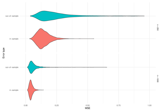
Figure 1: In-sample and out-of-sample errors for the model where $(Z_{1},\dots,Z_{7})\sim N_{7}(0,\boldsymbol{I})$, $Y=\sin(2\pi Z_{1})+\varepsilon$ with $\varepsilon\sim N(0,1)$ independently of $Z_{1},\dots,Z_{7}$, and regressions are performed using mgcv; see Section 6.1 for more details on this setup.

As the PCM may be thought of as the GCM applied to a transformed $X$, we would hope to obtain a standard Gaussian limit for $T$ as in the case of the regular GCM test statistic. Given that the transformation is designed to result in large values of $T$ under an alternative, we would perform a one-sided test by rejecting when $T$ exceeds the appropriate normal quantile. Unfortunately however, the theory that guarantees asymptotic validity of the GCM test statistic does not apply in our case: it would require ${\mathrm{Var}}(\{Y-m(Z)\}\{\widehat{f}(X,Z)-m_{\widehat{f}}(Z)\}\,|\,\widehat{f})$, i.e. the (square of the) target of the denominator, to be bounded away from zero under the null. But $f$ is identically $0$ under the null, so $\widehat{f}$ and hence the above variance, and also both numerator and denominator of our test statistic, should all converge to $0$.

To see why we can expect a standard Gaussian limit for our test statistic despite this apparent degeneracy, consider a linear model setting where $(X,Y,Z)\in{\mathbb{R}}\times{\mathbb{R}}\times{\mathbb{R}}^{d}$ are related through

$$Y=\beta X+Z^{\top}\boldsymbol{\gamma}+\varepsilon\qquad\text{and}\qquad X=Z^{\top}\boldsymbol{\eta}+\xi,$$ (7)

with $\beta=0$ and ${\mathbb{E}}(\varepsilon\,|\,Z)={\mathbb{E}}(\xi\,|\,Z)=0$. If we form estimates $\widehat{h}$ and $\widehat{m}$ using ordinary least squares, and for simplicity set $\widehat{v}\equiv 1$ when forming $\widehat{f}$, then $\widehat{f}(x,z)=\widehat{h}(x,z)$ takes the form $\widehat{\beta}x+z^{\top}\widetilde{\boldsymbol{\delta}}$ for some $(\widehat{\beta},\widetilde{\boldsymbol{\delta}})\in{\mathbb{R}}\times{\mathbb{R}}^{d}$. Note that both $\widehat{\beta}$ and $\|\widetilde{\boldsymbol{\delta}}\|_{2}$ are of stochastic order $1/\sqrt{n}$.

Let us write $\widehat{\boldsymbol{\gamma}}$ and $\widehat{\boldsymbol{\eta}}$ for the regression estimates of $\boldsymbol{\gamma}$ and $\boldsymbol{\eta}$ respectively. The next step of our procedure involves regressing each of $(Y_{i})_{i=1}^{n}$ and $\bigl{(}\widehat{f}(X_{i},Z_{i})\bigr{)}_{i=1}^{n}$ onto $(Z_{i})_{i=1}^{n}$. The residuals from the latter regression take the form $\widehat{\beta}\{Z_{i}^{\top}(\boldsymbol{\eta}-\widehat{\boldsymbol{\eta}})+\xi_{i}\}$, so in our case

$$L_{i}=\widehat{\beta}\{Z_{i}^{\top}(\boldsymbol{\gamma}-\widehat{\boldsymbol{\gamma}})+\varepsilon_{i}\}\{Z_{i}^{\top}(\boldsymbol{\eta}-\widehat{\boldsymbol{\eta}})+\xi_{i}\}.$$

Thus, although $L_{i}$ and hence its standard deviation would be of order $1/\sqrt{n}$ due to the factor of $\widehat{\beta}$, writing $L_{i}^{\prime}:=L_{i}/|\widehat{\beta}|$, we see that our test statistic is of the form $\mathrm{sgn}(\widehat{\beta})T^{\prime}$, where $T^{\prime}$ is a version of $T$ in (6) with $L_{i}$ replaced by $L_{i}^{\prime}$. But $L_{i}^{\prime}$ is an order 1 quantity (in contrast of $L_{i}$), so under mild conditions $n^{-1/2}\sum_{i=1}^{n}L_{i}^{\prime}$ will have a non-degenerate Gaussian limit, yielding a standard Gaussian limit for $T^{\prime}$. As $\widehat{\beta}$ is independent of $T^{\prime}$, having been constructed on $\mathcal{D}_{2}$, the final test statistic $T$ will also converge to a standard Gaussian.

While this argument provides a heuristic justification for the asymptotic validity of our proposed test under a simple linear model, there remain challenges in extending the basic intuition of this example to more general settings. In the above, it was possible to isolate the randomness from $\widehat{f}$ simply via the sign of $\widehat{\beta}$, which helps bypass the $0/0$ issue. However, it is by no means straightforward to deal with the limits of the form $0/0$ in a nonparametric setting where $\widehat{f}$ is entangled with other sources of randomness in a complicated way. Moreover, in nonparametric settings one needs to put more effort into ensuring that the convergence rates of $\widehat{f}$, $\widehat{m}$ and $\widehat{m}_{\widehat{f}}$ are fast enough that the bias term is asymptotically negligible. In this process, we are obliged to handle a nested regression problem that has rarely been touched in the literature with a few exceptions (e.g. Kennedy,, 2020).

2.2 PCM algorithm

Our PCM approach developed in Section 2.1 is set out in Algorithm 1, with some recommendations for the constructions of $\widehat{h}$ and $\widehat{v}$ that we discuss in Sections 2.2.1 and 2.2.2 below. In Section 2.2.3, we then put forward a version of the PCM using multiple sample splits that we recommend using in practice.

Algorithm 1 Projected Covariance Measure: single sample split

Input: Data $(X_{i},Y_{i},Z_{i})_{i=1}^{2n}$, significance level $\alpha\in(0,1)$, partition of $[2n]=\mathcal{I}_{1}\cup\mathcal{I}_{2}$ into index sets $\mathcal{I}_{1}$ and $\mathcal{I}_{2}$, each of size $n$.
Options: Regression methods for each of the regressions.
Define: $\mathcal{D}_{j}=(X_{i},Y_{i},Z_{i})_{i\in\mathcal{I}_{j}}$ for $j\in[2]$.

1:Form $\widehat{h}$.

1. Regress $Y$ onto $(X,Z)$ using $\mathcal{D}_{2}$ to give fitted regression function $\widehat{g}$.

2. If $\widehat{g}$ can be modified so that all components involving only $Z$ are set to $0$, let $\widetilde{g}$ be this modified version of $\widehat{g}$. Alternatively, set $\widetilde{g}:=\widehat{g}$.

3. Regress $\widetilde{g}(X,Z)$ onto $Z$ using $\mathcal{D}_{2}$ to give fitted regression function $\widetilde{m}$, and then set $\widetilde{h}(x,z):=\widetilde{g}(x,z)-\widetilde{m}(z)$.

4. Compute

   $$\widehat{\rho}:=\frac{1}{n}\sum_{i\in\mathcal{I}_{2}}\bigl{\{}Y_{i}-\widehat{g}(X_{i},Z_{i})+\widetilde{g}(X_{i},Z_{i})-\widetilde{m}(Z_{i})\bigr{\}}\widetilde{h}(X_{i},Z_{i}),$$

   and set $\widehat{h}(x,z):=\mathrm{sgn}(\widehat{\rho})\widetilde{h}(x,z)$,

2:Form $\widehat{v}$.

1. Regress $\{Y-\widehat{g}(X,Z)\}^{2}$ onto $(X,Z)$ using $\mathcal{D}_{2}$ to give $\widetilde{v}$.

2. Define $a:[0,\infty)\to[0,\infty]$ by

   $$a(c):=\frac{1}{n}\sum_{i\in\mathcal{I}_{2}}\frac{\{Y_{i}-\widehat{g}(X_{i},Z_{i})\}^{2}}{\max\{\widetilde{v}(X_{i},Z_{i}),0\}+c}.$$

   If $a(0)\leq 1$, set $\hat{c}:=0$; otherwise find $\hat{c}$ by solving $a(c)=1$. Set $\widehat{v}(x,z):=\max\{\widetilde{v}(x,z),0\}+\hat{c}$.

3:Compute test statistic.

1. Set $\widehat{f}(x,z):=\widehat{h}(x,z)/\widehat{v}(x,z)$ and regress $\widehat{f}(X,Z)$ onto $Z$ using $\mathcal{D}_{1}$, giving $\widehat{m}_{\widehat{f}}$.

2. Regress $Y$ onto $Z$ using $\mathcal{D}_{1}$ to give $\widehat{m}$.

3. For $i\in\mathcal{I}_{1}$ set $L_{i}:=\{Y_{i}-\widehat{m}(Z_{i})\}\{\widehat{f}(X_{i},Z_{i})-\widehat{m}_{\widehat{f}}(Z_{i})\}$ and let

   $$T:=\frac{\frac{1}{\sqrt{n}}\sum_{i\in\mathcal{I}_{1}}L_{i}}{\sqrt{\frac{1}{n}\sum_{i\in\mathcal{I}_{1}}L_{i}^{2}-\bigl{(}\frac{1}{n}\sum_{i\in\mathcal{I}_{1}}L_{i}\bigr{)}^{2}}}.$$

4:Reject $H_{0}$ if $T>z_{1-\alpha}$.

2.2.1 Choice of $\widehat{h}$

We would like $\widehat{h}(X,Z)$ to be close to $h(X,Z)={\mathbb{E}}(Y\,|\,X,Z)-{\mathbb{E}}(Y\,|\,Z)$ in order to maximise the power of the procedure. There are several ways of estimating $h$, with perhaps the most obvious being simply to take the difference of the estimated regression functions $\widehat{g}$ and $\check{m}$ from regressing $Y$ on each of $(X,Z)$ and $Z$. An alternative approach is based on observing that $h(X,Z)=g(X,Z)-{\mathbb{E}}\bigl{(}g(X,Z)\,|\,Z\bigr{)}$ where $g(X,Z):={\mathbb{E}}(Y\,|\,X,Z)$. This suggests subtracting not $\check{m}$ but the output of regressing $\widehat{g}(X,Z)$ onto $Z$. An advantage of this latter approach is that we are free to subtract any function $r$ of $Z$ from $\widehat{g}(X,Z)$ prior to this second regression onto $Z$, as we also have $h(X,Z)=g(X,Z)-r(Z)-{\mathbb{E}}\bigl{(}g(X,Z)-r(Z)\,|\,Z\bigr{)}$. Thus for example if $\widehat{g}(x,z)=\widehat{g}_{x}(x)+\widehat{g}_{z}(z)$, then we may form an estimate of $h(X,Z)$ as the residuals from regressing $\widehat{g}_{x}(X)$ onto $Z$. This second regression can then focus on removing any $Z$ signal in $\widehat{g}_{x}(X)$, rather than also having to cancel out $\widehat{g}_{z}(Z)$. We do not make the claim that this always makes a large improvement on the first approach, and indeed for certain regression methods such as ordinary least squares (OLS), both approaches are identical and the ‘cancellation’ is automatic. Nevertheless, we find the approach of Step 1 of Algorithm 1 to be a sensible default choice.

In Step 1(iv) we make a final modification to the estimate thus constructed by potentially flipping its sign. The rationale for this is as follows: under an alternative, we have that ${\mathbb{E}}[\{Y-{\mathbb{E}}(Y\,|\,Z)\}h(X,Z)]=\tau>0$. As a basic check then, we can see if an empirical version of this inequality, with $\widehat{h}$ taking place of $h$ and an estimate of ${\mathbb{E}}(Y\,|\,Z)$ replacing the population quantity, holds; if not, we can at least flip the sign of $\widehat{h}$. This does not require performing any further regressions to estimate ${\mathbb{E}}(Y\,|\,Z)$: noting the identity ${\mathbb{E}}(Y\,|\,Z)={\mathbb{E}}\{{\mathbb{E}}(Y\,|\,X,Z)-r(Z)\,|\,Z\}+r(Z)$, observe that $\widetilde{m}$ in Step 1(iii) is an estimate of the first of these quantities with $r(Z)=\widehat{g}(X,Z)-\widetilde{g}(X,Z)$, where $\widetilde{g}$ is defined in Step 1(ii). When using OLS for each of the regressions, $\widehat{\rho}$ is guaranteed to be non-negative, so no sign flip is performed.

In high-dimensional settings, we would typically use a sparsity-inducing regression method such as the Lasso (Tibshirani,, 1996). Considering the simple case where $X$ is univariate, this can result in the coefficient for $X$ being set exactly to zero, and so the recommended construction of $\widehat{h}$ given above would simply produce the zero function. While not a problem for Type I error control, as our convention (see Section 1.3) is not to reject the null when $L_{i}=0$ for all $i$, it is wasteful in terms of power and a better approach here would be to leave the coefficient for $X$ unpenalised. More generally for multivariate $X$, we can additionally regress on the first principal component of $X$ for example, and leave this unpenalised.

2.2.2 Choice of $\widehat{v}$

A natural way to form $\widehat{v}$ is to regress the square of the residuals from regressing $Y$ onto $(X,Z)$, and this is what we recommend in Step 2(i) of Algorithm 1 to produce $\widetilde{v}$. An issue is that while $v$ is clearly non-negative, and expected to be positive everywhere, $\widetilde{v}$ may in fact be negative. Equally problematic is the possibility that $\widetilde{v}$ is very close to $0$ at some $(X_{i},Z_{i})$, as then taking $\widehat{v}=\widetilde{v}$, we would have $\widehat{f}(X_{i},Z_{i})$ very large and hence $\widehat{f}(X_{i},Z_{i})-\widehat{m}_{\widehat{f}}(Z_{i})$ and $L_{i}$ may be greatly inflated and dominate the test statistic. To mitigate these problems, we modify $\widetilde{v}$ by taking the positive part of our initial estimate, and then adding a non-negative constant $\hat{c}$. This constant is chosen such that $a(\hat{c})$ (see Step 2(ii) of Algorithm 1) is at most $1$, the rationale coming from the population level identity ${\mathbb{E}}[\{Y-{\mathbb{E}}(Y\,|\,X,Z)\}^{2}/v(X,Z)]=1$. We also note that estimation of the conditional variance $v$ is not critical for good power properties. For example, in Section 5 we show that simply setting $\widehat{v}\equiv 1$ delivers minimax rate optimal power in a fully nonparametric setting; however the power properties may improve empirically by a constant factor; see Section 3.1.

2.2.3 Multiple sample splitting

The single sample split in Algorithm 1 crucially ensures independence between $\widehat{f}$ and the remaining data $\mathcal{D}_{1}$, but has the consequence of introducing unwanted additional randomness into the test statistic. This means that two practitioners with the same data may reach different conclusions about whether or not they should reject the null if they use different randomisation seeds. To circumvent this issue, we advocate applying the single split PCM to multiple splits of the data, and averaging the resulting test statistics, as summarised in Algorithm 2. An alternative to working with the averaged test statistic would be to combine the $p$-values of the individual tests, for which several methods are available, ranging from twice the average or median of $p$-values to the Bonferroni method (e.g. Vovk and Wang,, 2020; DiCiccio et al.,, 2020; Meinshausen et al.,, 2009, and references therein). However, our experience is that these approaches tend to be overly conservative, and typically lose power compared to considering a single test. Instead, we propose to compare the averaged test statistic $\bar{T}$ to a standard Gaussian quantile, as with the single split test statistic $T$. We expect this to be conservative, as by Jensen’s inequality, $\bar{T}$ is less than or equal to $T$ in the convex ordering, so for example ${\mathrm{Var}}(\bar{T})\leq{\mathrm{Var}}(T)$. However, in practice it does tend to improve slightly on the power of a single-split test, while at the same time having the important benefit of derandomising it. Recently Guo and Shah, (2023) proposed an approach for calibrating test statistics formed through multiple sample splitting using a form of subsampling that asymptotically yields a size equal to the chosen significance level i.e. the resulting test is not conservative; we leave further investigation of this approach to future work.

Algorithm 2 Projected Covariance Measure: multiple sample splits (recommended)

Input: Data $(X_{i},Y_{i},Z_{i})_{i=1}^{2n}$, significance level $\alpha\in(0,1)$, number of splits $B$.
Options: Regression methods for each of the regressions.

1:Form complementary pairs of index sets $\{(\mathcal{I}_{1}^{(b)},\mathcal{I}_{2}^{(b)}):b\in[B]\}$ each of size $n$, where $\mathcal{I}_{1}^{(b)}\cup\mathcal{I}_{2}^{(b)}=[2n]$.

2:For $b\in[B]$, apply Algorithm 1 with index sets $\mathcal{I}_{1}^{(b)},\mathcal{I}_{2}^{(b)}$ to produce test statistic $T^{(b)}$.

3:Define $\bar{T}:=\sum_{b=1}^{B}T^{(b)}/B$ and reject $H_{0}$ if $\bar{T}>z_{1-\alpha}$.

3 Linear models

In this section we study our PCM methodology in the context of a linear model for $Y$ on $X$ and $Z$. We begin with the simplest version of this setup, where we assume that $g(x,z):={\mathbb{E}}(Y\,|\,X=x,Z=z)$ is a linear function that we estimate using ordinary least squares. This is not the sort of challenging setting where we would envision applying the PCM in practice, as clearly a $t$-test (modified to account for potential heteroscedasticity) would suffice to test for the significance of $X$. We nevertheless present it to show that in contrast to the general methodologies put forward by Williamson et al., (2022) and Dai et al., (2022), here our method has power against $n^{-1/2}$-alternatives. In Section 3.2 below, we show that for both low- and high-dimensional $Z$, we retain Type I error control even under an arbitrary model for $X$ and when using an essentially arbitrary estimated projection $\widehat{f}$.

3.1 Linear projection function

We consider a family of $\mathcal{P}$ of joint distributions $P$ of $(X,Y,Z)\in\mathbb{R}\times\mathbb{R}\times\mathbb{R}^{d}$ satisfying the linear model

$$Y=\beta_{P}X+\boldsymbol{\gamma}_{P}^{\top}Z+\zeta_{P},$$ (8)

where $\beta_{P}\in\mathbb{R}$ and $\boldsymbol{\gamma}_{P}\in\mathbb{R}^{d}$ are regression coefficients and $\zeta_{P}$ is a random noise term with ${\mathbb{E}}_{P}(\zeta_{P}\,|\,X,Z)=0$. We further impose the following moment conditions on $\mathcal{P}$.

Assumption 1.

1. There exist $C,\delta>0$ such that

   $$\sup_{P\in\mathcal{P}}\max\bigl{\{}{\mathbb{E}}_{P}(\|Z\|_{\infty}^{4+\delta}),{\mathbb{E}}_{P}(|Y|^{4+\delta}),{\mathbb{E}}_{P}(|X|^{4+\delta})\bigr{\}}\leq C.$$

2. ${\mathbb{E}}_{P}(ZZ^{\top})\in\mathbb{R}^{d\times d}$ is invertible, and writing $\boldsymbol{\eta}_{P}:={\mathbb{E}}_{P}(ZZ^{\top})^{-1}{\mathbb{E}}_{P}(XZ)$, $\xi_{P}:=X-\boldsymbol{\eta}_{P}^{\top}Z$, $\boldsymbol{\Theta}_{P}:={\mathbb{E}}_{P}(ZZ^{\top}\xi_{P}^{2})$, and $\boldsymbol{\Sigma}_{P}^{XZ}:={\mathbb{E}}_{P}(WW^{\top})$ where $W:=(X,Z)\in\mathbb{R}\times\mathbb{R}^{d}$, there exists $c>0$ such that

   $$\inf_{P\in\mathcal{P}}\min\{{\mathrm{Var}}_{P}(\zeta_{P}\,|\,X,Z),{\mathrm{Var}}_{P}(\xi_{P}),\lambda_{\min}(\boldsymbol{\Sigma}_{P}^{XZ}),\lambda_{\min}(\boldsymbol{\Theta}_{P})\}\geq c.$$

Proposition 1.

Consider a version of the PCM setting $\widehat{v}\equiv 1$ and using OLS for each of the regressions involved for a family of distributions $\mathcal{P}$ satisfying Assumption 1 and (8). Let $\mathcal{P}_{1}(\kappa):=\{P\in\mathcal{P}:|\beta_{P}|\geq\kappa/\sqrt{n}\}$. Given any $\alpha\in(0,1)$, we have

$$\lim_{\kappa\rightarrow\infty}\lim_{n\to\infty}\inf_{P\in\mathcal{P}_{1}(\kappa)}{\mathbb{P}}_{P}(T>z_{1-\alpha})=1.$$

Proposition 1 gives the reassuring conclusion that in the simplest of settings, our general PCM framework, when used with appropriately chosen regression methods, can match up to a constant the power properties of a $t$-test tailored to this setting. In fact it turns out that the context is simple enough for us to derive an asymptotic power expression for our test. We present such an analysis in Section S5 of the supplementary material for a version of our test that uses $n_{1}$ and $n_{2}$ (with $n_{1}+n_{2}=2n$) observations in $\mathcal{D}_{1}$ and $\mathcal{D}_{2}$ respectively, rather than the equal split that we consider here. This shows that the optimal splitting ratio depends on the unknown signal strength, and therefore supports a default choice of $n_{1}=n_{2}=n$ for simplicity. We also provide a simulation study in Section S6.1 of the supplementary material where we compare the local power properties of the PCM, the Williamson et al., (2022) test and the $F$-test with a robust variance estimator.

3.2 A general estimated projection

We next consider a situation where the model is unspecified under the alternative, whereas $Y$ has a linear relationship with $Z$ under the null of conditional mean independence. In this case, it is reasonable to employ a flexible regression method, such as neural networks or random forests, to estimate the projection $f$. Our goal here is to identify conditions on estimators, including $\widehat{f}$, under which the proposed test controls the Type I error. It turns out that, given a specified null model, the problem of testing whether $X$ is significant is closely connected to goodness-of-fit testing for the null model, and we are able to exploit this connection to study the asymptotic Type I error of the proposed test.

Consider first the case of low-dimensional $Z$. Let $\mathcal{P}_{0}$ denote a family of distributions of $(X,Y,Z)$ under the null where $Z\in\mathbb{R}^{d}$ has an arbitrary distribution and suppose that $Y=\boldsymbol{\gamma}_{P}^{\top}Z+\varepsilon_{P}$, where ${\mathbb{E}}_{P}(\varepsilon_{P}\,|\,X,Z)=0$. Then $m_{P}(z)=\boldsymbol{\gamma}_{P}^{\top}Z$ and it is reasonable to use a linear regression model for $\widehat{m}$. We will suppose that the regressions yielding $\widehat{m}$ and $\widehat{m}_{\widehat{f}}$ in Algorithm 1 are performed using OLS, whereas we will leave the regression choices involved in the construction of $\widehat{f}$ arbitrary. We define $T_{\mathrm{OLS}}$ as the resulting test statistic, and make the following assumptions on $\mathcal{P}_{0}$ to ensure uniform asymptotic normality of the test statistic.

Assumption 2.

1. There exist $\delta\in(0,2]$, $c,C>0$ such that ${\mathbb{E}}_{P}(\varepsilon_{P}^{2}\,|\,X,Z)\geq c$ and ${{\mathbb{E}}_{P}(|\varepsilon_{P}|^{2+\delta}\,|\,X,Z)\leq C}$ for all $P\in\mathcal{P}_{0}$.

2. For $i\in[n]$, let $u_{n,i}:=\widehat{f}(X_{i},Z_{i})-\widehat{m}_{\widehat{f}}(Z_{i})$ and $\upsilon_{n,i}:=u_{n,i}/\bigl{(}\sum_{i^{\prime}=1}^{n}u_{n,i^{\prime}}^{2}\bigr{)}^{1/2}$. Assume that $\max_{i\in[n]}|\upsilon_{n,i}|=o_{\mathcal{P}_{0}}(1)$ and $\sum_{i=1}^{n}\upsilon_{n,i}^{2}=1+o_{\mathcal{P}_{0}}(1)$.

3. Letting $\boldsymbol{\widehat{\gamma}}$ denote the coefficient from the $\widehat{m}$ regression, assume that $\max_{i\in[n]}\|Z_{i}\|_{\infty}\cdot\|\boldsymbol{\widehat{\gamma}}-\boldsymbol{\gamma}_{P}\|_{1}=o_{\mathcal{P}_{0}}(1)$.

Part (a) of Assumption 2 concerns conditional moments of $\varepsilon$, and is used to establish the asymptotic normality of a suitably normalised version of the numerator of $T_{\mathrm{OLS}}$. In contrast to prior work on goodness-of-fit testing, e.g. Janková et al., (2020), we do not assume that the conditional variance of $\varepsilon$ is constant. Assumption 2(b) asks for no individual $|\upsilon_{n,i}|$ to be significantly larger than the others, and, for large enough $n$, that at least one of $\{u_{n,i}:i\in[n]\}$ is non-zero for all $P\in\mathcal{P}_{0}$, so $\widehat{f}(X,Z)$ is not constant in $X$. The latter condition is important for establishing the asymptotic normality of our test statistic, but is not crucial for Type I error control. Indeed, when $u_{n,i}=0$ for all $i\in[n]$, the test statistic is zero, and we do not reject the null. Finally, in settings where, for example each $Z_{i}$ has a uniformly bounded $(2+\delta)$th moment for some $\delta>0$, we have $\max_{i\in[n]}\|Z_{i}\|_{\infty}\lesssim n^{1/(2+\delta)}$ and $\|\boldsymbol{\widehat{\gamma}}-\boldsymbol{\gamma}_{P}\|_{1}\lesssim n^{-1/2}$ with high probability, and in that case Part (c) of Assumption 2 is satisfied.

Proposition 2 (Low-dimensional $Z$).

Suppose in the above setting that Assumption 2 holds and that all OLS estimators exist almost surely. Then the test statistic $T_{\mathrm{OLS}}$ converges to $N(0,1)$ uniformly over $\mathcal{P}_{0}$; i.e.,

$$\sup_{P\in\mathcal{P}_{0}}\sup_{t\in\mathbb{R}}\big{|}{\mathbb{P}}_{P}(T_{\mathrm{OLS}}\leq t)-\Phi(t)\big{|}\rightarrow 0.$$

Under the conditions of Proposition 2, the test that rejects the null when $T_{\mathrm{OLS}}>z_{1-\alpha}$ is uniformly asymptotically of size $\alpha$. We also note that the only requirement imposed on the projection $\widehat{f}$ is that it satisfies Assumption 2(b). Janková et al., (2020) also consider this condition, providing supporting empirical evidence in general, and introducing a specific procedure to guarantee that the condition holds.

We now extend these ideas and the setting described above Assumption 2 to the case where the dimension of $Z$ is potentially larger than the sample size. Here, the least squares estimator is not necessarily well-defined, so we construct $\widehat{m}$ and $\widehat{m}_{\widehat{f}}$ using the Lasso or one of its variants. Letting $\boldsymbol{\widehat{\gamma}}$ denote the coefficients from the $\widehat{m}$ regression, the motivation for this comes from the decomposition

$$\sum_{i=1}^{n}(Y_{i}-\boldsymbol{\widehat{\gamma}}^{\top}Z_{i})u_{n,i}=\sum_{i=1}^{n}\varepsilon_{P,i}u_{n,i}-\delta_{\mathrm{bias}},$$ (9)

where $\delta_{\mathrm{bias}}:=\sum_{i=1}^{n}(\boldsymbol{\widehat{\gamma}}-\boldsymbol{\gamma}_{P})^{\top}Z_{i}u_{n,i}$. This bias term is no longer exactly zero as for the least squares estimators considered in Proposition 2, but Hölder’s inequality will nevertheless guarantee that it is sufficiently small for our purposes as long as

$$\|\boldsymbol{\widehat{\gamma}}-\boldsymbol{\gamma}_{P}\|_{1}\cdot\bigg{\|}\sum_{i=1}^{n}Z_{i}\upsilon_{n,i}\bigg{\|}_{\infty}=o_{\mathcal{P}_{0}}(1).$$ (10)

We denote the test statistic as described in Algorithm 1 in this context by $T_{\mathrm{Lasso}}$. The next proposition is the analogue of Proposition 2 for $T_{\mathrm{Lasso}}$.

Proposition 3 (High-dimensional $Z$).

Suppose in the above setting that Assumption 2 and condition (10) hold. Then

$$\sup_{P\in\mathcal{P}_{0}}\sup_{t\in\mathbb{R}}\big{|}{\mathbb{P}}_{P}(T_{\mathrm{Lasso}}\leq t)-\Phi(t)\big{|}\rightarrow 0.$$

In order to ensure that condition (10) holds, one can use the square-root Lasso (Belloni et al.,, 2011; Sun and Zhang,, 2012), as suggested by Janková et al., (2020). In particular, for $\lambda_{\mathrm{sq}}>0$, we set $\widehat{m}_{\widehat{f}}(z)=\boldsymbol{\widehat{\eta}}_{\mathrm{sq}}^{\top}z$ where

$$\boldsymbol{\widehat{\eta}}_{\mathrm{sq}}:=\operatorname*{argmin}_{\boldsymbol{\eta}\in\mathbb{R}^{d}}\bigg{\{}\biggl{(}\frac{1}{n}\sum_{i=1}^{n}\bigl{(}\widehat{f}(X_{i},Z_{i})-\boldsymbol{\eta}^{\top}Z_{i}\bigr{)}^{2}\biggr{)}^{1/2}+\lambda_{\mathrm{sq}}\|\boldsymbol{\eta}\|_{1}\bigg{\}}.$$

With this choice of $\boldsymbol{\widehat{\eta}}_{\mathrm{sq}}$ and by letting $\lambda_{\mathrm{sq}}=c_{\mathrm{sq}}\sqrt{(\log d_{Z})/n}$ for some constant $c_{\mathrm{sq}}>0$, the Karush–Kuhn–Tucker conditions for the square-root Lasso guarantee that $\|\sum_{i=1}^{n}Z_{i}\upsilon_{n,i}\|_{\infty}\leq c_{\mathrm{sq}}\sqrt{\log d_{Z}}$. Furthermore, under appropriate conditions, the Lasso estimator $\boldsymbol{\widehat{\gamma}}$ has an error bound $\|\boldsymbol{\widehat{\gamma}}-\boldsymbol{\gamma}_{P}\|_{1}\lesssim s\sqrt{(\log d_{Z})/n}$ with high probability, where $s$ denotes the number of non-zero coefficients of $\boldsymbol{\gamma}_{P}$ (e.g. Corollary 6.2 of Bühlmann and van de Geer,, 2011). Therefore, in this setting, condition (10) is satisfied provided that $s(\log d_{Z})/\sqrt{n}\rightarrow 0$.

4 General theory

In this section, we present general conditions ensuring uniform asymptotic validity and power of the test, primarily by imposing assumptions on the performance of the regressions involved. To facilitate our analysis, it is helpful to study a slight modification of the test as presented in Algorithm 1, where we form $\widehat{m}$ and $\widehat{m}_{\widehat{f}}$ on an independent auxiliary sample. In principle, we may accomplish this by further splitting $\mathcal{D}_{1}$ into two, and using one part to train $\widehat{m}$ and $\widehat{m}_{\widehat{f}}$, and the other to compute the test statistic. Moreover, we can exchange the roles of the two parts and average the resulting test statistics, a process known as cross-fitting (Chernozhukov et al.,, 2018), which then guarantees no loss in efficiency from this additional sample split. However, for the reasons discussed in Section 2.1 we do not recommend performing this further sample split in practice.

The following quantities relating to the performances of the regression methods $\widehat{m}$ and $\widehat{m}_{\widehat{f}}$ will play a key role in our results. Let us introduce

$$\varepsilon_{P,i}:=Y_{i}-m_{P}(Z_{i}),\qquad\xi_{P,i}:=\widehat{f}(X_{i},Z_{i})-m_{P,\widehat{f}}(Z_{i}),$$ (11)

for $i\in[n]$, and an analogous version of (11) without a subscript $i$. Further, define

$$\sigma_{P}^{2}:={\mathrm{Var}}_{P}\bigl{(}\xi_{P}\,|\,\widehat{f}\bigr{)},$$ (12)

as well as

$$\mathcal{E}_{P,1}:=\frac{1}{n}\sum_{i=1}^{n}\{m_{P}(Z_{i})-\widehat{m}(Z_{i})\}^{2}\quad\text{and}\quad\mathcal{E}_{P,2}:=\frac{1}{n\sigma_{P}^{2}}\sum_{i=1}^{n}\{m_{P,\widehat{f}}(Z_{i})-\widehat{m}_{\widehat{f}}(Z_{i})\}^{2}.$$ (13)

The second MSPE $\mathcal{E}_{P,2}$ in the display above is normalised by the variance of the errors $\xi_{P,i}$ featuring in the corresponding regression. Under the null, we expect this variance to be small as $\widehat{f}$ is then estimating a zero function, and consequently $\mathcal{E}_{P,2}$ may be inflated relative to the unnormalised version of this quantity. On the other hand, as $\widehat{f}$ is small, we can expect that the unnormalised MSPE is particularly small. For example, writing $\mathcal{P}$ for the simple null linear model considered in (7), we would have

$$\frac{1}{n}\sum_{i=1}^{n}\{m_{P,\widehat{f}}(Z_{i})-\widehat{m}_{\widehat{f}}(Z_{i})\}^{2}=O_{\mathcal{P}}(n^{-2})\qquad\text{and}\qquad 1/\sigma_{P}^{2}=O_{\mathcal{P}}(n),$$

giving $\mathcal{E}_{P,2}=O_{\mathcal{P}}(n^{-1})$.

4.1 Type I error control

We consider the following assumption regarding general Type I error control.

Assumption 3.

Consider a class of null distributions $\mathcal{P}_{0}$ of $(X,Y,Z)$ on $\mathcal{X}\times\mathbb{R}\times\mathcal{Z}$ with ${\mathbb{E}}_{P}(Y\,|\,X,Z)={\mathbb{E}}_{P}(Y\,|\,Z)$ for which there exists $c>0$ such that $\inf_{P\in\mathcal{P}_{0}}{\mathbb{E}}_{P}(\varepsilon_{P}^{2}\,|\,X,Z)\geq c,$ and the following hold:

1. $\sup_{P\in\mathcal{P}_{0}}{\mathbb{P}}_{P}(\sigma_{P}^{2}=0)=o(1)$.

2. The product of the MSPEs satisfies $\mathcal{E}_{P,1}\mathcal{E}_{P,2}=o_{\mathcal{P}_{0}}(n^{-1})$.

3. The weighted

   MSPEs scaled by $\sigma_{P}^{2}$ satisfy

   $$\frac{1}{n\sigma_{P}^{2}}\sum_{i=1}^{n}\{m_{P}(Z_{i})-\widehat{m}(Z_{i})\}^{2}\xi_{P,i}^{2} =o_{\mathcal{P}_{0}}(1),$$

   $$\frac{1}{n\sigma_{P}^{2}}\sum_{i=1}^{n}\{m_{P,\widehat{f}}(Z_{i})-\widehat{m}_{\widehat{f}}(Z_{i})\}^{2}\varepsilon_{P,i}^{2} =o_{\mathcal{P}_{0}}(1).$$

4. There exists $\delta\in(0,2]$ such that ${\mathbb{E}}_{P}\bigl{(}|\varepsilon_{P}\xi_{P}|^{2+\delta}\,|\,\widehat{f}\bigr{)}/\sigma_{P}^{2+\delta}=o_{\mathcal{P}_{0}}(n^{\delta/2})$.

Part (a) of Assumption 3 asks that $\widehat{f}(X,Z)$ is not exactly constant in $X$ (even though we may expect it not to vary too much with $X$, for the reasons explained in the discussion in Section 2.1). Part (b) should be regarded as the primary restriction on $\mathcal{P}_{0}$, and along with (c), relates directly to the performance of the user-chosen regression methods involved in the construction of the PCM. As alluded to above, in a simple linear model setting, we can expect $\mathcal{E}_{P,1}\mathcal{E}_{P,2}=O_{\mathcal{P}_{0}}(n^{-2})$, which certainly satisfies the condition. The rate requirement on the product of MSPEs is however sufficiently slow to also accommodate nonparametric models; see Section 5. We note that the deterministic condition $\sup_{P\in\mathcal{P}_{0}}\{{\mathbb{E}}_{P}(\mathcal{E}_{P,1}){\mathbb{E}}_{P}(\mathcal{E}_{P,2})\}=o(n^{-1})$ is sufficient to guarantee part (b), as can be verified via Markov’s inequality and the Cauchy–Schwarz inequality. If in addition there exists $C>0$ such that ${\mathrm{Var}}_{P}(\xi_{P}\,|\,Z,\widehat{f})\leq C\sigma_{P}^{2}$ and ${\mathrm{Var}}_{P}(\varepsilon_{P})\leq C$, then (c) is guaranteed when $\widehat{m}$ and $\widehat{m}_{\widehat{f}}$ satisfy the simple consistency property $\sup_{P\in\mathcal{P}_{0}}\max\bigl{\{}{\mathbb{E}}_{P}(\mathcal{E}_{P,1}),\,{\mathbb{E}}_{P}(\mathcal{E}_{P,2})\bigr{\}}=o(1)$. Part (d) is a conditional Lyapunov condition, and is used to apply the central limit theorem for triangular arrays. A sufficient condition for this to hold when $\delta<2$ is that $\sup_{P\in\mathcal{P}_{0}}{\mathbb{E}}_{P}(|\varepsilon_{P}|^{(8+4\delta)/(2-\delta)})<\infty$ and ${\mathbb{E}}_{P}(|\xi_{P}|^{4}\,|\,\widehat{f})/\sigma_{P}^{4}=o_{\mathcal{P}_{0}}(n^{2\delta/(2+\delta)})$, which can be verified by Hölder’s inequality with conjugate exponents $p=4/(2-\delta)$ and $q=4/(2+\delta)$. The latter condition holds under an $L_{2}$–$L_{4}$ norm equivalence (e.g. Mendelson and Zhivotovskiy,, 2020) for $\xi_{P}$, and is certainly be satisfied if $\xi_{P}$ is log-concave conditional on $\widehat{f}$ (Lovász and Vempala,, 2007, Thm. 5.22).

Theorem 4 (Asymptotic normality under the null of a general procedure).

Suppose that Assumption 3 holds over a class of null distributions $\mathcal{P}_{0}$. Then

$$\sup_{P\in\mathcal{P}_{0}}\sup_{t\in\mathbb{R}}\bigl{|}{\mathbb{P}}_{P}(T\leq t)-\Phi(t)\bigr{|}\rightarrow 0.$$

The proof of Theorem 4 can be found in Section S1.4 of the supplementary material, which formalises the brief explanation of asymptotic normality laid down in Section 2.1. The above result indicates that the asymptotic normality of $T$ (hence the validity of the PCM test) is largely determined by the predictive performance of regression models used in construction of the test statistic.

Although we have stated Theorem 4 for the variant of our PCM procedure where $\widehat{m}$ and $\widehat{m}_{\widehat{f}}$ are formed on an auxiliary sample, it turns out that the conclusion holds more generally. Indeed, it follows from the proof that under Assumption 3, the abstract condition (S2) on our procedure suffices. In addition to being trivially satisfied when $\widehat{m}$ is formed on an auxiliary sample, (S2) holds for the practical version of our test where $\widehat{m}$ and $\widehat{m}_{\widehat{f}}$ are formed on $\mathcal{D}_{1}$ provided either that $X\mbox{${}\perp\mkern-11.0mu\perp{}$}Y\,|\,Z$ or that $\widehat{m}$ is a linear smoother. See Proposition S12 in Section S2.2 of the supplementary material for more details. Moreover our numerical results in Sections 6 and S6.2 demonstrate that Type I error can continue to be well-controlled in settings where $X\mbox{${}\not\!\perp\mkern-11.0mu\perp{}$}Y\,|\,Z$ and $\widehat{m}$ is not a linear smoother.

4.2 Power properties

When studying the power properties of our test, we restrict attention to a subset of alternatives that are separated from null distributions characterised by Assumption 4 below.

Assumption 4.

Given a positive sequence $(\epsilon_{n})_{n\in\mathbb{N}}$, let $\bigl{(}\mathcal{P}_{1}(\epsilon_{n})\bigr{)}_{n\in\mathbb{N}}$ denote a sequence of collections of alternative distributions such that

$$\inf_{P\in\mathcal{P}_{1}(\epsilon_{n})}\tau_{P}\geq\epsilon_{n}.$$

Further, suppose that there exists $C>0$ with

$$\limsup_{n\to\infty}\sup_{P\in\mathcal{P}_{1}(\epsilon_{n})}\max\{{\mathrm{Var}}_{P}(Y\,|\,X,Z),h_{P}(X,Z)\}\leq C,$$

and that the following conditions are satisfied:

1. There exists $\beta_{1}>0$ such that $\mathcal{E}_{P,1}=O_{\mathcal{P}_{1}(\epsilon_{n})}(n^{-\beta_{1}})$.

2. There exists $\beta_{2}>0$ such that $\mathcal{E}_{P,2}=O_{\mathcal{P}_{1}(\epsilon_{n})}(n^{-\beta_{2}})$.

3. There exists $\rho>0$ such that

   $$\sup_{P\in\mathcal{P}_{1}(\epsilon_{n})}{\mathbb{P}}_{P}\Bigl{(}{\mathrm{Corr}}_{P}\bigl{(}h_{P}(X,Z),\xi_{P}\,|\,\widehat{f}\bigr{)}\leq\rho\Bigr{)}=o(1).$$

In addition to the rate requirements on MSPEs in (a) and (b), condition (c) requires $\xi_{P}$, the population residuals from regressing our estimated projection $\widehat{f}$ onto $Z$, to be positively correlated with $h_{P}$ with high probability (there is no need for the correlation to approach $1$). To interpret (c), it is helpful to consider a stronger version of this condition with $\widehat{f}(X,Z)$ replacing $\xi_{P}$; to see that this results in a stronger condition, note that ${\mathbb{E}}_{P}\bigl{(}h_{P}(X,Z)\xi_{P}\,|\,\widehat{f}\bigr{)}={\mathbb{E}}_{P}\bigl{(}h_{P}(X,Z)\widehat{f}(X,Z)\,|\,\widehat{f}\bigr{)}$ and ${\mathbb{E}}(\xi_{P}^{2}\,|\,\widehat{f})={\mathbb{E}}_{P}\bigl{[}{\mathrm{Var}}_{P}\bigl{(}\widehat{f}(X,Z)\,|\,Z,\widehat{f}\bigr{)}\,|\,\widehat{f}\bigr{]}\leq{\mathbb{E}}\bigl{(}\widehat{f}(X,Z)^{2}\,|\,\widehat{f}\bigr{)}$. This stronger assumption still permits $\widehat{f}$ to be an inconsistent estimator of the true $f_{P}(X,Z)=h_{P}(X,Z)/{\mathrm{Var}}_{P}(Y\,|\,X,Z)$ in that it only requires them to be positively correlated, with probability approaching one.

The flexibility afforded by this assumption relies on using regression method $\widehat{m}_{\widehat{f}}$ being scale equivariant in the sense that

$$\widehat{m}_{a\cdot\widehat{f}}(Z)=a\cdot\widehat{m}_{\widehat{f}}(Z)$$ (14)

for all $a>0$; this is a mild condition, however, that is satisfied by many regression methods.

We can now state the main result of this subsection.

Theorem 5.

Assume that $\widehat{m}_{\widehat{f}}$ is scale equivariant in the sense that it satisfies (14) and consider the sequence of classes of distributions in Assumption 4, where

$$\epsilon_{n}\cdot n^{\min\{1,\beta_{1}+\beta_{2}\}}\rightarrow\infty.$$ (15)

Then for any $\alpha\in(0,1)$,

$$\inf_{P\in\mathcal{P}_{1}(\epsilon_{n})}{\mathbb{P}}_{P}(T>z_{1-\alpha})\rightarrow 1.$$

Theorem 5 shows that if $\beta_{1}+\beta_{2}\geq 1$, as may be expected if $m$ and $m_{\widehat{f}}$ are sufficiently smooth, then the rate $\epsilon_{n}$ is going to be driven by Assumption 4(c). It is well-known that an optimal convergence rate in terms of the squared prediction error under Hölder smoothness $s$ (Definition S21) is $n^{-2s/(2s+d_{Z})}$ (e.g., Nemirovski,, 2000; Györfi et al.,, 2002). If we assume that $m$ and $\sigma_{P}^{-1}m_{\widehat{f}}$ have Hölder smoothness $s$, and $\widehat{m}_{\widehat{f}}$ is scale equivariant as in (14), one may satisfy Assumptions 4(a) and 4(b) with $\beta_{1}=\beta_{2}=2s/(2s+d_{Z})$. In this setting, $\beta_{1}+\beta_{2}$ is greater than or equal to 1 provided that $s\geq d_{Z}/2$.

It is possible to derive a version of Theorem 5 for the test as described in Algorithm 1 that does not employ the additional sample splitting we are considering here. The only change is that (15) becomes $\epsilon_{n}\cdot n^{\min\{1,\beta_{1},\beta_{2}\}}\rightarrow\infty$; however we believe the version of Theorem 5 above is more in line with the behaviour to be expected in practice, and empirically we find the version of the test in Algorithm 1 to provide better discrimination between null and alternatives in finite samples.

5 Series estimators

Following the theory in the previous section for a general regression method, we will now provide more concrete results for a specific class, namely spline estimators. In particular, our interest is to identify conditions under which our test is uniformly asymptotically valid and attains near-optimal power in a nonparametric setting. A formal power analysis, however, is complicated by the fact that $\widehat{m}$ and $\widehat{m}_{\widehat{f}}$ are computed on the same subsample as our test statistic. We therefore consider a slightly modified test statistic that leverages ideas from the literature on cross-fitting. Throughout this section we assume that $(X,Z)\in[0,1]^{d_{X}}\times[0,1]^{d_{Z}}$ and set $d:=d_{X}+d_{Z}$.

Due to our additional sample splitting, we will require two additional independent samples of size $n$, so that we have $\mathcal{D}_{1},\ldots,\mathcal{D}_{4}$ in total. In Section S4 of the supplementary material, we give a self-contained description of spline spaces and their tensor product B-spline bases, containing all the results that we require for our analysis. Given a spline order $r\in\mathbb{N}$ (i.e. degree $r-1$) and $N\in\mathbb{N}_{0}$ equi-spaced interior knots in each dimension, we denote by $\mathcal{S}_{r,N}^{d_{Z}}$ the corresponding spline space on $[0,1]^{d_{Z}}$, and by $\boldsymbol{\phi}^{Z}$ its $d_{Z}$-tensor B-spline basis, which consists of $K_{Z}:=(N+r)^{d_{Z}}$ basis functions. Writing $\mathcal{S}_{r,N}^{d_{X}}$ for the corresponding spline space on $[0,1]^{d_{X}}$ with $d_{X}$-tensor B-spline basis $\boldsymbol{\phi}^{X}$, having $K_{X}:=(N+r)^{d_{X}}$ basis functions, we can define the $d$-tensor product basis $\boldsymbol{\phi}(x,z):=\boldsymbol{\phi}^{X}(x)\otimes\boldsymbol{\phi}^{Z}(z)$ for $\mathcal{S}_{r,N}^{d}$, where $\boldsymbol{u}\otimes\boldsymbol{v}:=\mathrm{vec}(\boldsymbol{u}\boldsymbol{v}^{\top})$, having $K_{XZ}:=K_{X}K_{Z}$ basis functions. Further, we let $\boldsymbol{\psi}$ denote the tensor product B-spline basis for $\mathcal{S}_{2r-1,N}^{d_{Z}}$, and write $\widetilde{K}_{Z}:=(N+2r-1)^{d_{Z}}$; the higher order of the spline basis functions that make up $\boldsymbol{\psi}$ affords better approximation properties that turn out to be useful for our theory.

The following description of the test statistic fixes notation and follows Algorithm 1 except that we fit $\widehat{m}_{\widehat{f}}$ on $\mathcal{D}_{3}$, $\widehat{m}$ on $\mathcal{D}_{4}$ and set $\widehat{v}\equiv 1$ for simplicity. We will also omit discussion of the sign correction step (Algorithm 1 1(iv)), since $\widehat{\rho}$ is always non-negative for the estimators considered below. We first regress $Y$ onto $\boldsymbol{\phi}(X,Z)$ using ordinary least squares (OLS) on $\mathcal{D}_{2}$, yielding an estimator $\boldsymbol{\widehat{\beta}}_{XZ}\in\mathbb{R}^{K_{XZ}}$, and set $\widehat{g}(x,z):=\boldsymbol{\widehat{\beta}}_{XZ}^{\top}\boldsymbol{\phi}(x,z)$. We then regress $\widehat{g}(X,Z)$ onto $\boldsymbol{\phi}(X,Z)$ using OLS on $\mathcal{D}_{2}$ again, to obtain an estimator $\boldsymbol{\widehat{\beta}}_{Z}\in\mathbb{R}^{K_{Z}}$, and set $\widetilde{m}(z):=\boldsymbol{\widehat{\beta}}_{Z}^{\top}\boldsymbol{\phi}^{Z}(z)$. Note that this is equivalent to regressing $Y$ onto $\boldsymbol{\phi}^{Z}(Z)$. We then define the projection $\widehat{f}(x,z):=\widehat{g}(x,z)-\widetilde{m}(z)$. Using the fact that $\boldsymbol{\phi}^{X}$ forms a partition of unity (Proposition S20(a) in the supplementary material), it follows that if we write $\widehat{\boldsymbol{\beta}}:=\boldsymbol{\widehat{\beta}}_{XZ}-\boldsymbol{1}\otimes\boldsymbol{\widehat{\beta}}_{Z}$, where $\boldsymbol{1}\in\mathbb{R}^{K_{X}}$ denotes a vector of ones, then $\widehat{f}(x,z)=\widehat{\boldsymbol{\beta}}^{\top}\boldsymbol{\phi}(x,z)$.

To estimate $m_{P,\widehat{f}}$, we regress $\widehat{f}(X,Z)$ onto $\boldsymbol{\psi}(Z)$ on $\mathcal{D}_{3}$ using OLS, giving $\widehat{m}_{\widehat{f}}$. Similarly, we estimate $m_{P}$ by regressing $Y$ onto $\boldsymbol{\psi}(Z)$ on $\mathcal{D}_{4}$ using OLS to give $\widehat{m}$. Given $\widehat{f}$, $\widehat{m}$ and $\widehat{m}_{\widehat{f}}$ as defined above, we compute the test statistic as in Algorithm 1 (on $\mathcal{D}_{1}$) and denote it by $T_{\mathrm{Spline}}$. In Theorem 6 in Section 5.1 below, we demonstrate that $T_{\mathrm{Spline}}$ enjoys uniform asymptotic Type I error control under appropriate regularity conditions, while Theorem 7 and Proposition 8 in Section 5.2 reveal that $T_{\mathrm{Spline}}$ can achieve the optimal testing rate for this problem.

5.1 Type I error control

We start by stating our main distributional assumptions, which rely on the definitions of Hölder spaces $\mathcal{H}_{s}^{d}$ and Hölder norms $\|\cdot\|_{\mathcal{H}_{s}}$ given in Definition S21.

Assumption 5.

Let $\mathcal{P}$ be a class of distributions of $(X,Y,Z)$ on $[0,1]^{d_{X}}\times\mathbb{R}\times[0,1]^{d_{Z}}$, and for $P\in\mathcal{P}$, let $g_{P}(x,z):={\mathbb{E}}_{P}(Y\,|\,X=x,Z=z)$. Assume that there exist $C\geq 1$ and $c\in(0,1]$ with the following properties:

1. For each $P\in\mathcal{P}$, we have ${\mathbb{E}}_{P}(\varepsilon_{P}^{2}\,|\,X,Z)\geq c$ and there exists $\delta\in(0,2]$ such that
   ${\mathbb{E}}_{P}(|\varepsilon_{P}|^{2+\delta}\,|\,X,Z)\leq C$.

2. For each $P\in\mathcal{P}$, the marginal distribution of $(X,Z)$ is absolutely continuous with respect to Lebesgue measure on $[0,1]^{d}$, with density $p_{P}$ satisfying $\sup_{(x,z)\in[0,1]^{d}}p_{P}(x,z)\leq C$ and $\inf_{(x,z)\in[0,1]^{d}}p_{P}(x,z)\geq c$.

3. Let $s\in(0,r]$ and let $p_{X|Z,P}(\cdot\,|\,z)$ denote the conditional density of $X$ given $Z=z$. Assume that for all $P\in\mathcal{P}$, we have $p_{X|Z,P}(x\,|\,\cdot)\in\mathcal{H}^{d_{Z}}_{s}$ for all $x\in[0,1]^{d_{X}}$, and that $m_{P}\in\mathcal{H}^{d_{Z}}_{s}$ and $g_{P}\in\mathcal{H}^{d}_{s}$, with

   $$\max\biggl{\{}\sup_{x\in[0,1]^{d_{X}}}\|p_{X|Z,P}(x,\cdot)\|_{\mathcal{H}_{s}},\|m_{P}\|_{\mathcal{H}_{s}},\|g_{P}\|_{\mathcal{H}_{s}}\biggr{\}}\leq C.$$

Assumption 5 is closely related to other assumptions commonly used in spline regression (e.g. Belloni et al.,, 2015; Ichimura and Newey,, 2015; Newey and Robins,, 2018). In order to state our Type I error control result for $T_{\mathrm{Spline}}$, it will be convenient to define the projection $\boldsymbol{\Pi}:\mathbb{R}^{K_{XZ}}\rightarrow\mathbb{R}^{K_{XZ}}$ by $\boldsymbol{\Pi}(\boldsymbol{x})\equiv\boldsymbol{\Pi}(x_{1},\ldots,x_{K_{XZ}}):=\boldsymbol{x}-\boldsymbol{1}\otimes\bar{\boldsymbol{x}}$, with $\bar{\boldsymbol{x}}=(\bar{x}_{1},\ldots,\bar{x}_{K_{Z}})$ given by $\bar{x}_{k}:=K_{X}^{-1}\sum_{\ell=1}^{K_{X}}x_{(k-1)K_{X}+\ell}$ for $k\in[K_{Z}]$.

Theorem 6 (Asymptotic normality of $T_{\mathrm{Spline}}$).

Suppose that Assumption 5 holds for a class of null distributions $\mathcal{P}_{0}$, i.e. a class of distributions that also satisfies ${\mathbb{E}}_{P}(Y\,|\,X,Z)={\mathbb{E}}_{P}(Y\,|\,Z)$ for every $P\in\mathcal{P}_{0}$. Assume that $\sup_{P\in\mathcal{P}_{0}}{\mathbb{P}}_{P}(\|\boldsymbol{\Pi}\boldsymbol{\widehat{\beta}}\|_{\infty}=0)=o(1)$ and that
$\boldsymbol{\Lambda}_{P}:={\mathbb{E}}_{P}\bigl{\{}{\mathrm{Cov}}_{P}\bigl{(}\boldsymbol{\phi}(X,Z)\,|\,Z\bigr{)}\bigr{\}}$ satisfies

$$\tilde{\lambda}_{\min}(\boldsymbol{\Lambda}_{P}):=\min_{\boldsymbol{x}\in\mathbb{R}^{K_{XZ}}:\boldsymbol{\Pi}\boldsymbol{x}=\boldsymbol{x},\|\boldsymbol{x}\|_{2}=1}\boldsymbol{x}^{\top}\boldsymbol{\Lambda}_{P}\boldsymbol{x}\geq\frac{c}{K_{XZ}},$$ (16)

for each $P\in\mathcal{P}_{0}$, where $c\in(0,1]$ is taken from Assumption 5. Finally, suppose that

$$nK_{XZ}\biggl{\{}\widetilde{K}_{Z}^{-2s/d_{Z}}+\frac{\widetilde{K}_{Z}}{n}\biggr{\}}^{2}\rightarrow 0$$ (17)

and

$$\frac{K_{XZ}^{1+2/\delta}}{n}\rightarrow 0$$ (18)

where $\delta$ is taken from Assumption 5. Then

$$\sup_{P\in\mathcal{P}_{0}}\sup_{t\in\mathbb{R}}\bigl{|}{\mathbb{P}}_{P}(T_{\mathrm{Spline}}\leq t)-\Phi(t)\bigr{|}\rightarrow 0.$$

The proof of Theorem 6 amounts to the verification of Assumption 3, which then allows us to apply our general Type I error control result, namely Theorem 4. In addition to Assumption 5, Theorem 6 imposes several additional conditions. The assumption that $\sup_{P\in\mathcal{P}_{0}}{\mathbb{P}}_{P}(\|\boldsymbol{\Pi}\boldsymbol{\widehat{\beta}}\|_{\infty}=0)=o(1)$ simply avoids degeneracy of the test statistic and is used to show that Assumption 3(a) is satisfied. If this condition is not satisfied, then since we defined $0/0:=0$ in the definition of our test statistic, it can be shown that

$$\liminf_{n\rightarrow\infty}\inf_{P\in\mathcal{P}_{0}}{\mathbb{P}}_{P}(|T_{\mathrm{Spline}}|\leq t)\geq\Phi(t)-\Phi(-t)$$

for all $t\geq 0$ (i.e. $|T_{\mathrm{Spline}}|$ is asymptotically stochastically dominated by the absolute value of a standard Gaussian random variable), so the test retains uniform asymptotic Type I error control provided that $\alpha\leq 1/2$.

Condition (16) can be regarded as a restricted minimum eigenvalue condition; for $\boldsymbol{x}\in\mathbb{R}^{K_{XZ}}$ with $\boldsymbol{\Pi}\boldsymbol{x}=0$, we have that $\boldsymbol{x}^{\top}\boldsymbol{\Lambda}_{P}\boldsymbol{x}=0$, but it turns out that we are able to restrict attention to the orthogonal complement of this subspace. Motivation for the form of this condition is provided by the fact that, writing $\boldsymbol{\Sigma}_{P}:={\mathbb{E}}_{P}\bigl{(}\boldsymbol{\phi}(X,Z)\boldsymbol{\phi}(X,Z)^{\top}\bigr{)}\in\mathbb{R}^{K_{XZ}\times K_{XZ}}$, we have

$$\tilde{\lambda}_{\min}(\boldsymbol{\Lambda}_{P})\leq\tilde{\lambda}_{\min}(\boldsymbol{\Sigma}_{P})\leq\lambda_{\max}(\boldsymbol{\Sigma}_{P})\leq C2^{d}K_{XZ}^{-1}$$

by Proposition S20(d). Moreover, Lemma S14 in Section S2.2 of the supplementary material shows that the assumption holds when $X$ and $Z$ are independent.

Condition (17) is used to show that parts (b) and (c) of Assumption 3 are satisfied while Condition (18) is used to show that part (d) of the assumption is satisfied. These conditions control the interplay between the growth rate of the number of basis functions, the smoothness $s$ of the regression functions and conditional densities and $\delta$. When choosing the knot spacing to minimise the mean-squared error of the involved regressions, we would choose $\widetilde{K}_{Z}$ and $K_{Z}$ of order $n^{d_{Z}/(2s+d_{Z})}$ and $K_{X}$ of order $n^{d_{X}/(2s+d_{Z})}$. Thus for (17) to hold, we need $s>d_{Z}+d_{X}/2$ and for (18) to hold, we need $\delta>2(d_{X}+d_{Z})/(2s-d_{X})$. Both of conditions could be weakened, at the expense of additional notational complexity, by choosing different knot spacings $N_{X}$ and $N_{Z}$ for the $d_{X}$- and $d_{Z}$-tensor B-spline bases $\boldsymbol{\phi}^{X}$ and $\boldsymbol{\phi}^{Z}$ for our spline spaces $\mathcal{S}_{r,N_{X}}^{d_{X}}$ and $\mathcal{S}_{r,N_{Z}}^{d_{Z}}$. Indeed, by taking $N_{X}$, and hence $K_{X}$, to be of constant order, while retaining the original choices of $K_{Z}$ and $\widetilde{K}_{Z}$, we see that (17) holds when $s>d_{Z}$ and (18) holds when $\delta>d_{Z}/s$ (so it would suffice for Assumption 5(a) to hold with $\delta=1$, provided again that $s>d_{Z}$).

5.2 Power and minimax lower bound

As mentioned at the beginning of this section, we employ additional sample splitting in the construction of $T_{\mathrm{Spline}}$. This turns out to be helpful in demonstrating the optimality of our test. To provide insight into the benefits of sample splitting in this context, consider two generic spline estimators $\widehat{g}_{1}$ and $\widehat{g}_{2}$ of unknown functions $g_{1}$ and $g_{2}$, respectively. Suppose that we would like to choose $\widehat{g}_{1}$ and $\widehat{g}_{2}$ to minimise the empirical cross-product error

$$\widehat{\theta}_{\mathrm{cross}}:=\frac{1}{n}\sum_{i=1}^{n}\{\widehat{g}_{1}(Z_{i})-g_{1}(Z_{i})\}\{\widehat{g}_{2}(Z_{i})-g_{2}(Z_{i})\}.$$ (19)

A naive way of approaching this problem is to construct $\widehat{g}_{1}$ and $\widehat{g}_{2}$ on the same dataset and to choose the number of spline functions so as to minimise the mean-squared error of each of $\widehat{g}_{1}$ and $\widehat{g}_{2}$. The Cauchy–Schwarz inequality then guarantees that the cross-product error is small as long as the mean-squared errors are small. However, this indirect approach returns a potentially suboptimal rate of convergence due to its “own observation” bias, which arises from using the same datasets to form $\widehat{g}_{1}$ and $\widehat{g}_{2}$. When employing auxiliary samples to construct $\widehat{g}_{1}$ and $\widehat{g}_{2}$ we can eliminate this bias; thus a more refined analysis of terms like $\widehat{\theta}_{\mathrm{cross}}$ that does not directly employ the Cauchy–Schwarz inequality can result in faster convergence rates; see for instance Proposition S32 in the supplementary material. Our main result in this section is as follows:

Theorem 7.

Let $\mathcal{P}$ be a class of distributions satisfying Assumption 5, and let $\mathcal{P}_{1}(\epsilon_{n}):=\{P\in\mathcal{P}:\tau_{P}\geq\epsilon_{n}\}$, where

$$\epsilon_{n}\cdot n^{\frac{4s}{4s+d}}\rightarrow\infty.$$ (20)

Further, assume that the tuning parameters are chosen such that $K_{X}\asymp n^{\frac{2d_{X}}{4s+d}}$ and $K_{Z}\asymp\widetilde{K}_{Z}\asymp n^{\frac{2d_{Z}}{4s+d}}$ and that $r\geq s\geq 3d/4$. Then

$$\inf_{P\in\mathcal{P}_{1}(\epsilon_{n})}{\mathbb{P}}_{P}(T_{\mathrm{Spline}}>z_{1-\alpha})\rightarrow 1.$$

Theorem 7 reveals that the test based on $T_{\mathrm{Spline}}$ has uniform asymptotic power 1 over a class of alternatives that are sufficiently separated from the null, as defined by $\mathcal{P}_{1}(\epsilon_{n})$.

We remark that in Theorem 7, we have operated in the context of a known smoothness parameter $s$ for theoretical purposes. It is possible to construct more involved tests that adapt to unknown smoothness levels following the strategy of Lepskiǐ, (1991) and Ingster, (2000), but we do not pursue this direction further.

The separation rate (20) cannot be improved further from a minimax perspective, as illustrated by the following lower bound result.

Proposition 8.

Consider a class of distributions, denoted by $\mathcal{P}$, that satisfy Assumption 5, and let $\mathcal{P}_{1}(\epsilon_{n}):=\{P\in\mathcal{P}:\tau_{P}\geq\epsilon_{n}\}$. Then, for a fixed level $\alpha\in(0,1/2)$, there exists $c>0$ such that if $\limsup_{n\rightarrow\infty}\epsilon_{n}\cdot n^{\frac{4s}{4s+d}}<c$, then any test $\phi$ having uniform asymptotic size at most $\alpha$ satisfies

$$\limsup_{n\rightarrow\infty}\inf_{P\in\mathcal{P}_{1}(\epsilon_{n})}{\mathbb{P}}_{P}(\phi=1)\leq\alpha+1/2.$$

Proposition 8 complements Theorem 7 by showing that when $\tau_{P}$ is a small constant multiple of $n^{-\frac{4s}{4s+d}}$, no test can achieve uniform consistency under Hölder smoothness. The proof of Proposition 8, which can be found in Section S1.8 of the supplementary material, follows a fairly standard argument (e.g. Ingster,, 1987; Arias-Castro et al.,, 2018) that bounds the $\chi^{2}$-divergence from a fixed null distribution to a mixture of distributions in the alternative class $\mathcal{P}_{1}(\epsilon_{n})$.

Despite the theoretical benefits described above, employing additional sample splitting may degrade the practical performance of the algorithm, especially in small sample scenarios. We therefore recommend using the PCM without this additional sample splitting in practice, and its finite-sample performance is investigated in the next section.

6 Numerical experiments

In this section, we present the results of several simulation experiments that investigate the empirical performances of both the recommended multiple sample splitting version of the PCM (see Algorithm 2) with $B=6$ splits, denoted by pcm, and the single split version (see Algorithm 1) denoted by pcm_ss. We compare our tests to various conditional (mean) independence tests in the literature listed below.

• The test based on the default $p$-value for a smooth when fitting a generalised additive model (GAM) using the mgcv-package in R (Wood,, 2013, 2017).

• The test resulting from applying the approach described in Williamson et al., (2022, Algorithm 3) and employing sample splitting and cross-fitting as implemented in the cv_vim function from the vimp-package in R (with $K=2$, resulting in $4$ folds).

• The kernel conditional independence test (Zhang et al.,, 2011) as implemented in the KCI function of the CondIndTests R package (Heinze-Deml et al.,, 2018); we use the Bayesian hyperparameter tuning option for sample sizes of at most $500$.

• The Generalised Covariance Measure (GCM) as described in Shah and Peters, (2020).

• The ‘fixed weight function’ variant of the Weighted Generalised Covariance Measure (wGCM) (Scheidegger et al.,, 2022) as implemented in the wgcm.fix function of the weightedGCM R package; we use $\texttt{weight.num}=7$ as in the simulations of the original paper.

• The ‘estimated weight function’ variant of the wGCM as implemented in the wgcm.est function of the weightedGCM R-package.

In all of our numerical simulations, rejection rates were estimated based on 2500 repetitions. The code for all of our experiments (including those in the supplementary material) is available on GitHub: https://github.com/ARLundborg/pcm_code/

6.1 Additive models

We first investigate Type I error control and power in setting where both ${\mathbb{E}}(Y\,|\,Z)$ and ${\mathbb{E}}(X\,|\,Z)$ are additive functions, and $Z\sim N_{7}(0,\boldsymbol{I})$. For the methods, including the PCM, requiring choices of regression procedures, we use a generalised additive model fitted using mgcv. We employ default parameters for the generalised additive models, as given in the smooth.terms and gam functions in the mgcv package), except that we choose $\lfloor(N-1)/d\rfloor$ basis functions (where $N$ and $d$ are the number of observations and predictors on which the model is trained, respectively). Since this is the largest number of basis functions per coordinate that can be taken without overparametrisation, this mitigates the risk of oversmoothing; as the fits are penalised, there is little risk of overfitting (Wood,, 2017). We consider null settings consisting of $n\in\{250,500,1000\}$ independent and identically distributed copies of $(X,Y,Z)$ where

$$X=\sin(2\pi Z_{1})+0.1\xi\quad\text{and}\quad Y=\sin(2\pi Z_{1})+\varepsilon.$$

and errors $\varepsilon$ and $\xi$ are independent $N(0,1)$ random variables, independent of $Z$. Such a setup is challenging for Type I error control as $X$ and $Y$ are highly correlated yet are conditionally independent given $Z$. Indeed we see from the left panel of Figure 2 that several of the tests are anti-conservative, most notably kci and gam, which we omit from further comparisons as their power properties would be hard to interpret given the high rejection rates under the null. The wgcm.est test is also somewhat anti-conservative, but considerably less so. In contrast, the pcm is conservative here. This is to be expected as the calibration following the multiple sample splits involved in its construction (Section 2.2.3) is typically conservative; the single split version pcm_ss appears to have rejection rates close to the nominal 5% mark as suggested by our theory.

We investigate the power properties of the PCM in the following settings, where as before, $\varepsilon$ and $\xi$ are independent and independent of $Z$, and moreover $\varepsilon\sim N(0,1)$.

1. $\xi\sim N(0,1)$, $X=\sin(2\pi Z_{1})+\xi$ and $Y=\sin(2\pi Z_{1})+0.2X^{2}+\varepsilon$.

2. $\xi+1\sim\textrm{Exp}(1)$, $X=\sin(2\pi Z_{1})-\sin(2\pi Z_{1})\xi$ and $Y=\sin(2\pi Z_{1})+0.4X^{2}+\varepsilon$.

3. $\xi\sim N(0,1)$, $X=\sin(2\pi Z_{1})+\xi$ and $Y=\sin(2\pi Z_{1})+0.4X^{2}Z_{2}+\varepsilon$.

The settings are chosen such that in setting 1: ${\mathbb{E}}\bigl{(}{\mathrm{Cov}}(X,Y\,|\,Z)\bigr{)}=0$ but ${\mathrm{Cov}}(X,Y\,|\,Z)\neq 0$, in setting 2: ${\mathrm{Cov}}(X,Y\,|\,Z)=0$ but $\tau\neq 0$ and in setting 3: there is only an interaction effect. We cannot expect this interaction effect to be picked up by methods that fit additive models, but we nevertheless include this setting to emphasise the fact that the success of the PCM and related methods is contingent on an appropriate choice of regression method; see also Section 6.2.

From the right-hand panels of Figure 2, we see that the pcm and wgsc exhibit good power in settings 1 and 2. wgcm.est also shows appreciable power in setting 1, though as expected has little power in setting 2 where ${\mathrm{Cov}}(X,Y\,|\,Z)=0$. For the reasons explained above, the PCM has no power in setting 3; in the next section we investigate the performance of the PCM when used in conjunction with a regression method capable of fitting to such regression functions.

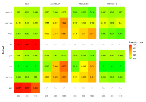
Figure 2: Rejection rates in the various settings considered in Section 6.1 looking at additive models for nominal 5%-level tests. Note that Alternative 3 has only an interaction effect, so we cannot expect methods that fit additive models to have power.

6.2 Non-additive models

In this section, we consider settings where the regression functions are non-additive and involve complex interactions. We use random forests (Breiman,, 2001) implemented in the ranger R package (Wright and Ziegler,, 2017) as our regression procedure for the methods considered. We use $500$ trees and set mtry equal to the number of predictors, with other tuning parameters set to be the defaults for the ranger function; the choice of mtry was made as this tended to give the smallest prediction errors in our preliminary experiments.

We consider null settings consisting of $n\in\{10^{4},2\cdot 10^{4},4\cdot 10^{4}\}$ independent and identically distributed copies of $(X,Y,Z)$ where $Z\sim N_{7}(0,\boldsymbol{I})$ as before,

$$X=\sin(2\pi Z_{1})(1+Z_{3})+\xi\quad\text{and}\quad Y=\sin(2\pi Z_{1})(1+Z_{3})+v(X)\varepsilon$$

with $\varepsilon$ and $\xi$ independent $N(0,1)$ random variables independent of $Z$, and $v(X):=0.5+\mathbbm{1}_{\{X>0\}}$ giving heteroscedastic errors for the $Y$ regression model. The larger sample sizes considered here reflect the difficulty of estimating the more complicated regression functions in these examples. Note that here we do not have $X\mbox{${}\perp\mkern-11.0mu\perp{}$}Y\,|\,Z$, but the conditional mean independence ${\mathbb{E}}(Y\,|\,X,Z)={\mathbb{E}}(Y\,|\,Z)$ does hold. The results are presented in Figure 3. We see that the multiple sample splitting version of the PCM maintains Type I error control, and is in fact slightly conservative. All other approaches considered appear to be anti-conservative to varying degrees: the wgsc approach is most clearly miscalibrated here, and we omit it from our alternative settings described below; wgcm.est and gcm are also fairly anti-conservative here but the rejection rates appear to be improving for increasing $n$.

We consider the following alternative settings, where as in Section 6.1, setting 2 has
${\mathrm{Cov}}(X,Y\,|\,Z)=0$, and setting 3 involves a pure interaction effect:

1. $\xi\sim N(0,1)$, $X=\sin(2\pi Z_{1})(1+Z_{3})+\xi$ and $Y=\sin(2\pi Z_{1})(1+Z_{3})+0.04X^{2}+v(X)\varepsilon$;

2. $\xi\sim\textrm{Exp}(1)$, $X=\sin(2\pi Z_{1})(1+Z_{3})-\sin(2\pi Z_{1})(\xi-1)$ and $Y=\sin(2\pi Z_{1})(1+Z_{3})+0.04X^{2}+v(X)\varepsilon$;

3. $\xi\sim N(0,1)$, $X=\sin(2\pi Z_{1})(1+Z_{3})+\xi$ and $Y=\sin(2\pi Z_{1})(1+Z_{3})+0.04X^{2}Z_{2}+v(X)\varepsilon$.

Among the methods considered, here only the PCM appear to have good power across the settings considered. The wgcm.est has reasonable power in setting 1, though this should be interpreted with some care given that Type I error is not very well controlled in the null settings. However in setting 2, wgcm.est is powerless as expected.

Figure 3: Rejection rates in the various settings considered in Section 6.2 on non-additive models for nominal 5%-level tests.

7 Conclusion

In this work we have introduced a general test statistic called the PCM for testing conditional mean independence that: (a) can leverage machine learning methods to yield provable uniform Type I error control across a class of null distributions where these methods have sufficiently good predictive ability; and (b) when used in conjunction with appropriate regression methods attains rate-optimal power in both the parametric setting of the linear model and fully nonparametric settings. We believe the PCM fills an important gap in the data analyst’s range of existing tools, which are unable simultaneously to achieve these desiderata. However, our work also offers several avenues for further work, some of which we mention below.

Verifying the general assumptions for other regression methods

We have verified Assumption 3 for linear regression in linear model settings, and nonparametric series estimators in fully nonparametric settings. Since we used the penalised regression splines of mgcv in several of our numerical experiments, it would be interesting to see for what classes $\mathcal{P}$ of distributions Assumption 3 is satisfied in that context. Similarly, it would be very interesting to ask the same question of random forests, which perform very well in our simulations; however this is likely to be challenging given the complex nature of the random forest procedure.

Aggregation of test statistics from multiple sample splits

Our proposal (Algorithm 2) to average test statistics from multiple sample splits and compare this to a standard Gaussian quantile works fairly well in practice, though in some cases appears to be overly conservative. It would be of interest to explore whether approaches such as that of Guo and Shah, (2023) can be employed here to calibrate the test more accurately and improve power.

Conditional independence testing

Although the problem of testing conditional independence has been studied more intensively than that of testing conditional mean independence, there do not exist many practical conditional independence tests that achieve the two desiderata mentioned at the beginning of this section. One starting point for constructing a such a test may be the fact that the conditional independence null $Y\mbox{${}\perp\mkern-11.0mu\perp{}$}X\,|\,Z$ may be viewed as the intersection of conditional mean independence nulls ${\mathbb{E}}\bigl{(}w(Y)\,|\,X,Z\bigr{)}={\mathbb{E}}\bigl{(}w(Y)\,|\,Z\bigr{)}$ where function $w$ ranges over all monotone functions, for example. It might therefore be interesting to investigate procedures that seek two ‘projections’: mappings $(X,Z)\to\widehat{f}(X,Z)$ and also $Y\mapsto\widehat{w}(Y)$, after which one may apply the GCM.

Confidence intervals

We have focused on the problem of testing conditional mean independence, but the problem of deriving confidence intervals for a parameter such as $\tau$ that is $0$ under our null is equally interesting. The pioneering work of Williamson et al., (2021) proposes an asymptotically optimal approach for this in the case where $\tau$ is bounded away from $0$. It would be interesting if the PCM could be used in conjunction with the proposal of Williamson et al., (2021) to extend the latter to yield confidence intervals with uniform coverage for all $\tau$.

In Sections S1 and S2 of the supplementary material, we include the proofs of all of our main results and related auxiliary lemmas. In Section S3, we present a detailed discussion of the test proposed by Williamson et al., (2022). In Section S4, we give a self-contained description of spline regression and related results that we use for our analysis in Section 5. Section S5 contains an analysis of the linear projections in Section 3 under more general assumptions. We also derive an exact asymptotic power function of our test in this setting. Section S6 contains the results from additional numerical experiments beyond those included in Section 6.

Throughout the supplementary material, for a positive semi-definite matrix $\boldsymbol{A}$, we write $\boldsymbol{A}^{-1}$ for its generalised inverse (i.e. its Moore–Penrose pseudo-inverse).

Appendix S1 Proofs

In our proofs we often suppress the dependence of quantities on $P$ for ease of notation.

S1.1 Proof of Proposition 1

There is no loss of generality in assuming that $\alpha\leq 1/2$, because for $\alpha>1/2$, we have $\mathbb{P}(T>z_{1-\alpha})\geq\mathbb{P}(T>z_{1/2})=\mathbb{P}(T>0)$. We start by checking the assumptions of Lemma S10 for the regressions of $Y$ on $X$ and $Z$ (of which $\widehat{\beta}$ is one component), $Y$ on $Z$ (yielding $\boldsymbol{\widehat{\theta}}$) and $X$ on $Z$ (yielding $\boldsymbol{\widehat{\eta}}$). Let $\delta^{\prime}:=\delta/2$.

Recalling that $W=(X,Z)$, we see that condition (i) of Lemma S10 is satisfied for the $Y$ on $X$ and $Z$ regression by our assumption on $\boldsymbol{\Sigma}^{XZ}$ and the fact that

$$\lambda_{\min}\bigl{(}{\mathbb{E}}(WW^{\top}\zeta^{2})\bigr{)}\geq c\lambda_{\min}(\boldsymbol{\Sigma}^{XZ})$$

by our assumption that ${\mathrm{Var}}(Y\,|\,X,Z)\geq c$. Condition (ii) is satisfied with $\delta=\delta^{\prime}$ by the Cauchy–Schwarz inequality and Jensen’s inequality.

By Assumption 1, condition (i) of Lemma S10 is satisfied for the $X$ on $Z$ regression. To see that condition (ii) is satisfied with $\delta=\delta^{\prime}$, we note that by the Cauchy–Schwarz inequality it suffices to check that ${\mathbb{E}}(|\xi|^{4+\delta})$ is bounded over $\mathcal{P}$. Letting $\boldsymbol{\Sigma}:={\mathbb{E}}(ZZ^{\top})$, we have

$${\mathbb{E}}(|\xi|^{4+\delta})\leq 2^{3+\delta}\Bigl{(}{\mathbb{E}}(|X|^{4+\delta})+\lambda_{\min}(\boldsymbol{\Sigma})^{-(4+\delta)}\|{\mathbb{E}}(XZ)\|_{2}^{4+\delta}{\mathbb{E}}(\|Z\|_{2}^{4+\delta})\Bigr{)}$$

which is bounded under Assumption 1.

To see that condition (i) of Lemma S10 is satisfied for the $Y$ on $Z$ regression, define $\boldsymbol{\theta}:={\mathbb{E}}(ZZ^{\top})^{-1}{\mathbb{E}}(YZ)\in{\mathbb{R}}^{d}$ and note that

$${\mathbb{E}}\bigl{(}ZZ^{\top}(Y-\boldsymbol{\theta}^{\top}Z)^{2}\bigr{)} ={\mathbb{E}}\bigl{(}ZZ^{\top}(\zeta+\beta X-\beta\boldsymbol{\eta}^{\top}Z)^{2}\bigr{)}$$

$$={\mathbb{E}}(ZZ^{\top}\zeta^{2})+\beta^{2}{\mathbb{E}}\bigl{(}ZZ^{\top}(X-\boldsymbol{\eta}^{\top}Z)^{2}\bigr{)},$$

so the minimum eigenvalue of ${\mathbb{E}}\bigl{(}ZZ^{\top}(Y-\boldsymbol{\theta}^{\top}Z)^{2}\bigr{)}$ is bounded below by $c\lambda_{\min}(\boldsymbol{\Sigma})$. Condition (ii) follows by similar arguments as those for the $X$ on $Z$ regression. We therefore deduce from Lemma S10 that (S49) holds with $\sigma_{\beta}^{2}$ given by the $(1,1)$th entry of the matrix $(\boldsymbol{\Sigma}^{XZ})^{-1}\mathbb{E}(WW^{\top}\zeta^{2})(\boldsymbol{\Sigma}^{XZ})^{-1}$, and that

$$\sqrt{n}\|\boldsymbol{\widehat{\eta}}-\boldsymbol{\eta}\|_{2}=O_{\mathcal{P}}(1)\quad\text{and}\quad\sqrt{n}\|\boldsymbol{\widehat{\theta}}-\boldsymbol{\theta}\|_{2}=O_{\mathcal{P}}(1).$$ (S1)

We now verify that the remaining parts of Assumption S1 are satisfied. First,

$$\sup_{P\in\mathcal{P}}{\mathbb{E}}\biggl{(}\Bigl{\|}\frac{1}{n}\sum_{i=1}^{n}Z_{i}\xi_{i}\Bigr{\|}_{2}^{2}\biggr{)}=\frac{1}{n}\sup_{P\in\mathcal{P}}{\mathbb{E}}\bigl{(}\|Z\xi\|_{2}^{2}\bigr{)}\leq\frac{1}{n}\sup_{P\in\mathcal{P}}{\mathbb{E}}(\|Z\|_{2}^{2})\cdot\sup_{P\in\mathcal{P}}{\mathbb{E}}(\xi^{2})\to 0,$$

so by Lemma S6 and (S1) we have that (S50) holds. Similar arguments show that (S51) is satisfied.

Next, (S1) shows that

$$\sqrt{n}\|\boldsymbol{\widehat{\eta}}-\boldsymbol{\eta}\|_{2}\|\boldsymbol{\widehat{\theta}}-\boldsymbol{\theta}\|_{2}=O_{\mathcal{P}}(n^{-1/2})=o_{\mathcal{P}}(1).$$

Moreover, by (S31) in the proof of Lemma S10 and Assumption 1, we have

$$\Bigl{\|}\frac{1}{n}\sum_{i=1}^{n}Z_{i}Z_{i}^{\top}\Bigr{\|}_{\mathrm{op}}\leq\Bigl{\|}\frac{1}{n}\sum_{i=1}^{n}Z_{i}Z_{i}^{\top}-\boldsymbol{\Sigma}\Bigr{\|}_{\mathrm{op}}+\|\boldsymbol{\Sigma}\|_{\mathrm{op}}=O_{\mathcal{P}}(1),$$

so (S52) is satisfied. The remaining conditions hold by similar arguments using the moment bounds established earlier, (S1) and Lemma S9.

To verify the remaining conditions of Proposition S34, we note that

$${\mathrm{Var}}(\varepsilon\xi)\geq{\mathbb{E}}\bigl{\{}{\mathrm{Var}}(\varepsilon\xi\,|\,X,Z)\bigr{\}}={\mathbb{E}}\bigl{\{}\xi^{2}{\mathrm{Var}}(Y\,|\,X,Z)\bigr{\}}\geq c^{2}.$$

Finally, the moment bound condition in Proposition S34 follows by Cauchy–Schwarz and the arguments above. The conclusion now follows from Proposition S34 together with the fact that $\psi_{\alpha,n}$ is an increasing function of $|\beta|$, so that

$$\psi_{\alpha,n}\geq\Phi\biggl{(}\frac{\kappa}{\sigma_{\beta}}\biggr{)}\cdot\Phi\biggl{(}z_{\alpha}+\frac{\kappa\sigma_{\xi}^{2}}{\sigma_{\varepsilon\xi}}\biggr{)}+\Phi\biggl{(}-\frac{\kappa}{\sigma_{\beta}}\biggr{)}\cdot\Phi\biggl{(}z_{\alpha}-\frac{\kappa\sigma_{\xi}^{2}}{\sigma_{\varepsilon\xi}}\biggr{)}\rightarrow 1$$

as $\kappa\rightarrow\infty$, as required.

S1.2 Proof of Proposition 2

Throughout this proof we work on the event that at least one $u_{n,1},\ldots,u_{n,n}$ is non-zero which is a set of uniform asymptotic probability $1$ by Assumption 2(b). Let $\boldsymbol{Z}:=(Z_{1}^{\top},\ldots,Z_{n}^{\top})^{\top}$, $\boldsymbol{P}:=\boldsymbol{Z}(\boldsymbol{Z}^{\top}\boldsymbol{Z})^{-1}\boldsymbol{Z}^{\top}$, $\boldsymbol{Y}:=(Y_{1},\ldots,Y_{n})^{\top}$, $\boldsymbol{\varepsilon}:=(\varepsilon_{1},\ldots,\varepsilon_{n})^{\top}$, $\boldsymbol{\widehat{f}}:=\bigl{(}\widehat{f}(X_{1},Z_{1}),\dots,\widehat{f}(X_{n},Z_{n})\bigr{)}^{\top}$ and $\boldsymbol{I}$ denote the $d\times d$ identity matrix. Since $\boldsymbol{P}$ is a matrix representing an orthogonal projection such that $\boldsymbol{Z}^{\top}(\boldsymbol{I}-\boldsymbol{P})$ is a zero vector, we have

$$\sum_{i=1}^{n}\{Y_{i}-\boldsymbol{\widehat{\gamma}}^{\top}Z_{i}\}\{\widehat{f}(X_{i},Z_{i})-\widehat{m}_{\widehat{f}}(Z_{i})\} =\boldsymbol{\widehat{f}}^{\top}(\boldsymbol{I}-\boldsymbol{P})\boldsymbol{Y}=\boldsymbol{\widehat{f}}^{\top}(\boldsymbol{I}-\boldsymbol{P})\boldsymbol{\varepsilon}$$

$$=\sum_{i=1}^{n}\varepsilon_{i}\{\widehat{f}(X_{i},Z_{i})-\widehat{m}_{\widehat{f}}(Z_{i})\}.$$

Based on the above identity, we have that

$$T_{\mathrm{OLS}}=\frac{\frac{1}{\sqrt{n}\nu}\sum_{i=1}^{n}\varepsilon_{i}u_{n,i}}{\sqrt{\frac{1}{n\nu^{2}}\sum_{i=1}^{n}(Y_{i}-\boldsymbol{\widehat{\gamma}}^{\top}Z_{i})^{2}u_{n,i}^{2}-\bigl{(}\frac{1}{n\nu}\sum_{i=1}^{n}\varepsilon_{i}u_{n,i}\bigr{)}^{2}}},$$

where

$$\nu:=\sqrt{\frac{1}{n}\sum_{i=1}^{n}{\mathbb{E}}(\varepsilon_{i}^{2}\,|\,X_{i},Z_{i})u_{n,i}^{2}}>0.$$

Let $\mathcal{F}_{n}$ denote the $\sigma$-algebra generated by $\widehat{f}$ and $\bigl{(}(X_{i},Z_{i})\bigr{)}_{i=1}^{n}$. Form the triangular array

$$W_{n,i}:=\frac{\varepsilon_{i}u_{n,i}}{\nu}$$

for $n\in\mathbb{N}$ and $i\in[n]$, and note that this satisfies the first three assumptions of Lemma S8, since $u_{n,i}$ is measurable with respect to $\mathcal{F}_{n}$. Finally, the fourth assumption of this lemma is also satisfied, because

$$\frac{1}{n^{1+\delta/2}} \sum_{i=1}^{n}{\mathbb{E}}(|W_{n,i}|^{2+\delta}\,|\,\mathcal{F}_{n})=\frac{1}{n^{1+\delta/2}\nu^{2+\delta}}\sum_{i=1}^{n}{\mathbb{E}}(|\varepsilon_{i}|^{2+\delta}\,|\,X_{i},Z_{i})|u_{n,i}|^{2+\delta}$$

$$\leq\frac{C}{c^{1+\delta/2}}\sum_{i=1}^{n}|\upsilon_{n,i}|^{2+\delta}\leq\frac{C}{c^{1+\delta/2}}\biggl{(}\sum_{i=1}^{n}|\upsilon_{n,i}|^{2}\biggr{)}\max_{i\in[n]}|\upsilon_{n,i}|^{\delta}=o_{\mathcal{P}_{0}}(1)$$

by Assumptions 2(a) and (b) and Lemmas S3 and S7. Lemma S8 thus yields that the numerator of $T_{\mathrm{OLS}}$ is uniformly asymptotically standard Gaussian.

For the denominator of $T_{\mathrm{OLS}}$, the uniform version of Slutsky’s theorem (Bengs and Holzmann,, 2019, Theorem 6.3) yields that $\frac{1}{n\nu}\sum_{i=1}^{n}\varepsilon_{i}u_{n,i}=o_{\mathcal{P}_{0}}(1)$. For the first term in the denominator of $T_{\mathrm{OLS}}$, we consider the decomposition

$$\frac{1}{n\nu^{2}}\sum_{i=1}^{n}(Y_{i}-\boldsymbol{\widehat{\gamma}}^{\top}Z_{i})^{2}u_{n,i}^{2}=\underbrace{\frac{1}{n\nu^{2}}\sum_{i=1}^{n}\varepsilon_{i}^{2}u_{n,i}^{2}}_{\textup{I}_{n}} +\underbrace{\frac{1}{n\nu^{2}}\sum_{i=1}^{n}\{(\boldsymbol{\widehat{\gamma}}-\boldsymbol{\gamma})^{\top}Z_{i}\}^{2}u_{n,i}^{2}}_{\textup{II}_{n}}$$

$$-\underbrace{\frac{2}{n\nu^{2}}\sum_{i=1}^{n}(\boldsymbol{\widehat{\gamma}}-\boldsymbol{\gamma})^{\top}Z_{i}\varepsilon_{i}u_{n,i}^{2}}_{\textup{III}_{n}}.$$

Similarly to our previous argument, define the triangular array $\tilde{W}_{n,i}:=W_{n,i}^{2}$ for $n\in\mathbb{N}$ and $i\in[n]$, and note that $(\tilde{W}_{n,i})_{n\in\mathbb{N},i\in[n]}$ satisfies the conditions of Lemma S9 with $\mu_{n}=1$ in that result, so $\textup{I}_{n}=1+o_{\mathcal{P}_{0}}(1)$. Now, by Hölder’s inequality,

$$|\textup{II}_{n}|\leq\frac{1}{n\nu^{2}}\|\boldsymbol{\widehat{\gamma}}-\boldsymbol{\gamma}\|_{1}^{2}\sum_{i=1}^{n}\|Z_{i}\|_{\infty}^{2}u_{n,i}^{2}\leq\frac{1}{c}\max_{i\in[n]}\|Z_{i}\|_{\infty}^{2}\|\boldsymbol{\widehat{\gamma}}-\boldsymbol{\gamma}\|_{1}^{2}\sum_{i=1}^{n}\upsilon_{n,i}^{2}=o_{\mathcal{P}}(1),$$

by Assumption 2 and Lemma S3. Finally, the Cauchy–Schwarz inequality yields that

$$|\textup{III}_{n}| \leq 2\sqrt{\frac{1}{n\nu^{2}}\sum_{i=1}^{n}\varepsilon_{i}^{2}u_{n,i}^{2}}\cdot\sqrt{\frac{1}{n\nu^{2}}\sum_{i=1}^{n}\{(\boldsymbol{\widehat{\gamma}}-\boldsymbol{\gamma})^{\top}Z_{i}\}^{2}u_{n,i}^{2}}=2\sqrt{\textup{I}_{n}}\cdot\sqrt{\textup{II}_{n}}=o_{\mathcal{P}}(1)$$

by Lemmas S3 and S7. The result follows by the uniform version of Slutsky’s theorem.

S1.3 Proof of Proposition 3

As in the proof of Proposition 2, we work on the event that at least one $u_{n,1},\ldots,u_{n,n}$ is non-zero, which is a set of uniform asymptotic probability $1$ by Assumption 2(b). Recall the definitions of $\nu$ from the proof of Proposition 2, and $\delta_{\mathrm{bias}}$ from just after (9). Our test statistic can be written as

$$T_{\mathrm{Lasso}}=\frac{\frac{1}{\sqrt{n}\nu}\sum_{i=1}^{n}\varepsilon_{i}u_{n,i}-\frac{1}{\sqrt{n}\nu}\delta_{\mathrm{bias}}}{\sqrt{\frac{1}{ns_{n}^{2}}\sum_{i=1}^{n}(Y_{i}-\boldsymbol{\widehat{\gamma}}^{\top}Z_{i})^{2}u_{n,i}^{2}-\bigl{(}\frac{1}{n\nu}\sum_{i=1}^{n}\varepsilon_{i}u_{n,i}+\frac{1}{n\nu}\delta_{\mathrm{bias}}\bigr{)}^{2}}}.$$

Following the proof of Proposition 2, we know that $\frac{1}{\sqrt{n}\nu}\sum_{i=1}^{n}\varepsilon_{i}u_{n,i}$ converges uniformly to $N(0,1)$. Further, by Assumption 2(a) and Hölder’s inequality, we have

$$\biggl{|}\frac{1}{\sqrt{n}\nu}\delta_{\mathrm{bias}}\biggr{|}\leq\frac{1}{c^{1/2}}\biggl{|}\sum_{i=1}^{n}(\boldsymbol{\widehat{\gamma}}-\boldsymbol{\gamma})^{\top}Z_{i}\upsilon_{n,i}\biggr{|}\leq\frac{1}{c^{1/2}}\|\boldsymbol{\widehat{\gamma}}-\boldsymbol{\gamma}\|_{1}\biggl{\|}\sum_{i=1}^{n}Z_{i}\upsilon_{n,i}\biggr{\|}_{\infty}=o_{\mathcal{P}_{0}}(1)$$

under condition (10). A uniform version of Slutsky’s theorem (Bengs and Holzmann,, 2019, Theorem 6.3) now yields that the numerator of $T_{\mathrm{Lasso}}$ is uniformly asymptotically standard Gaussian. We can repeat the arguments of Proposition 2 to show that the denominator is $1+o_{\mathcal{P}_{0}}(1)$ under Assumption 2, so the uniform version of Slutsky’s theorem yields the desired result.

S1.4 Proof of Theorem 4

We prove the result under the given assumptions but instead of assuming that $\widehat{m}$ and $\widehat{m}_{\widehat{f}}$ are formed on an auxiliary sample, we let $R_{ij}:={\mathbb{E}}\bigl{(}M_{i}M_{j}\,|\,(X_{i^{\prime}},Z_{i^{\prime}})_{i^{\prime}=1}^{n}\bigr{)}-{\mathbb{E}}\bigl{(}M_{i}M_{j}\,|\,(Z_{i^{\prime}})_{i^{\prime}=1}^{n}\bigr{)}$ for $i\neq j$, where $M_{i}:=m(Z_{i})-\widehat{m}(Z_{i})$, and assume that

$$\frac{1}{n\sigma_{n}^{2}}\sum_{i\neq j}\bigl{|}{\mathbb{E}}\bigl{(}R_{ij}\xi_{i}\xi_{j}\,|\,(Z_{i^{\prime}})_{i^{\prime}=1}^{n},\widehat{f}\bigr{)}\bigr{|}=o_{\mathcal{P}_{0}}(1).$$ (S2)

In Proposition S12 we show that this condition is satisfied if $\widehat{m}$ is formed out of sample as in the statement of Theorem 4. We also show in that result that (S2) is satisfied if $\widehat{m}$ is a linear smoother or if $X\mbox{${}\perp\mkern-11.0mu\perp{}$}Y\,|\,Z$. Define $\nu^{2}:={\mathrm{Var}}(\varepsilon\xi)$ and note that $\nu^{2}\geq c\sigma^{2}$. Throughout this proof we work on the event $\Omega_{0}:=\{\sigma\neq 0\}$, which satisfies $\mathbb{P}(\Omega_{0}^{c})=o_{\mathcal{P}_{0}}(1)$ by Assumption 3(a). Define

$$T^{(\mathrm{N})}:=\frac{\frac{1}{\sqrt{n}}\sum_{i=1}^{n}L_{i}}{\nu}\quad\text{and}\quad T^{(\mathrm{D})}:=\frac{\sqrt{\frac{1}{n}\sum_{i=1}^{n}L_{i}^{2}-\bigl{(}\frac{1}{n}\sum_{i=1}^{n}L_{i}\bigr{)}^{2}}}{\nu},$$

so that $T=T^{(\mathrm{N})}/T^{(\mathrm{D})}$. We will show that $T^{(\mathrm{N})}$ converges uniformly in distribution to $N(0,1)$ and $|T^{(\mathrm{D})}-1|=o_{\mathcal{P}_{0}}(1)$, which yields the desired result by combining Lemma S7 and the uniform version of Slutsky’s lemma (Bengs and Holzmann,, 2019, Theorem 6.3).

Define $\widetilde{M}_{i}:=m_{\widehat{f}}(Z_{i})-\widehat{m}_{\widehat{f}}(Z_{i})$ for $i\in[n]$ and note that

$$T^{(\mathrm{N})}=\underbrace{\frac{1}{\sqrt{n}\nu}\sum_{i=1}^{n}M_{i}\widetilde{M}_{i}}_{a_{n}}+\underbrace{\frac{1}{\sqrt{n}\nu}\sum_{i=1}^{n}\widetilde{M}_{i}\varepsilon_{i}}_{b_{n}}+\underbrace{\frac{1}{\sqrt{n}\nu}\sum_{i=1}^{n}M_{i}\xi_{i}}_{c_{n}}+\underbrace{\frac{1}{\sqrt{n}\nu}\sum_{i=1}^{n}\varepsilon_{i}\xi_{i}}_{U_{n}}.$$ (S3)

By the Cauchy–Schwarz inequality,

$$a_{n}\leq\sqrt{\frac{1}{cn}\biggl{(}\sum_{i=1}^{n}M_{i}^{2}\biggr{)}\biggl{(}\frac{1}{\sigma^{2}}\sum_{i=1}^{n}\widetilde{M}_{i}^{2}\biggr{)}}=o_{\mathcal{P}_{0}}(1),$$

by Assumption 3(b).

To see that $b_{n}=o_{\mathcal{P}_{0}}(1)$, we note that

$$b_{n}^{2}=\frac{1}{n\nu^{2}}\sum_{i=1}^{n}\widetilde{M}_{i}^{2}\varepsilon_{i}^{2}+\frac{1}{n\nu^{2}}\sum_{i\neq j}\widetilde{M}_{i}\widetilde{M}_{j}\varepsilon_{i}\varepsilon_{j}$$ (S4)

and the first term is $o_{\mathcal{P}_{0}}(1)$ by Assumption 3(c). Now, for $i\neq j$,

$${\mathbb{E}}(Y_{i}Y_{j}\,|\,X_{i},X_{j},Z_{i},Z_{j})={\mathbb{E}}(Y_{i}\,|\,X_{i},Z_{i}){\mathbb{E}}(Y_{j}\,|\,X_{j},Z_{j})=m(Z_{i})m(Z_{j}),$$

using the fact that $m(Z)={\mathbb{E}}(Y\,|\,Z)={\mathbb{E}}(Y\,|\,X,Z)$ under $\mathcal{P}_{0}$. Hence,

$${\mathbb{E}}(\varepsilon_{i}\varepsilon_{j}\,|\,X_{i},X_{j},Z_{i},Z_{j}) ={\mathbb{E}}\bigl{\{}\bigl{(}Y_{i}-m(Z_{i})\bigr{)}\bigl{(}Y_{j}-m(Z_{j})\bigr{)}\,|\,X_{i},X_{j},Z_{i},Z_{j}\bigr{\}}$$

$$={\mathbb{E}}(Y_{i}Y_{j}\,|\,X_{i},X_{j},Z_{i},Z_{j})-m(Z_{i})m(Z_{j})=0.$$

It follows that

$${\mathbb{E}}\Bigl{(}\frac{1}{n\nu^{2}}\sum_{i\neq j}\widetilde{M}_{i}\widetilde{M}_{j}\varepsilon_{i}\varepsilon_{j} \biggm{|}(X_{i^{\prime}},Z_{i^{\prime}})_{i^{\prime}=1}^{n},\widehat{f},\widehat{m}_{\widehat{f}}\Bigr{)}$$

$$=\frac{1}{n\nu^{2}}\sum_{i\neq j}\widetilde{M}_{i}\widetilde{M}_{j}{\mathbb{E}}(\varepsilon_{i}\varepsilon_{j}\,|\,X_{i},X_{j},Z_{i},Z_{j})=0,$$

and we deduce by Lemmas S6 and S7 that $b_{n}=o_{\mathcal{P}_{0}}(1)$.

To see that $c_{n}=o_{\mathcal{P}_{0}}(1)$, we proceed as above and write

$$c_{n}^{2}=\frac{1}{n\nu^{2}}\sum_{i=1}^{n}M_{i}^{2}\xi_{i}^{2}+\frac{1}{n\nu^{2}}\sum_{i\neq j}M_{i}M_{j}\xi_{i}\xi_{j},$$

where we again note that the first term is $o_{\mathcal{P}_{0}}(1)$ by Assumption 3(c). Moreover,

$${\mathbb{E}}\Bigl{(}\frac{1}{n\nu^{2}}\sum_{i\neq j}M_{i}M_{j}\xi_{i}\xi_{j} \biggm{|}(Z_{i^{\prime}})_{i^{\prime}=1}^{n},\widehat{f}\Bigr{)}$$

$$=\frac{1}{n\nu^{2}}\sum_{i\neq j}{\mathbb{E}}\bigl{\{}{\mathbb{E}}\bigl{(}M_{i}M_{j}\,|\,(X_{i^{\prime}},Z_{i^{\prime}})_{i^{\prime}=1}^{n}\bigr{)}\xi_{i}\xi_{j}\,|\,(Z_{i^{\prime}})_{i^{\prime}=1}^{n},\widehat{f}\bigr{\}}$$

$$=\frac{1}{n\nu^{2}}\sum_{i\neq j}{\mathbb{E}}(R_{ij}\xi_{i}\xi_{j}\,|\,(Z_{i^{\prime}})_{i=1}^{n},\widehat{f}),$$

where the last equality holds since

$${\mathbb{E}}\bigl{\{}{\mathbb{E}}\bigl{(}M_{i}M_{j}\,|\,(Z_{i^{\prime}})_{i^{\prime}=1}^{n}\bigr{)}\xi_{i}\xi_{j}\,|\,(Z_{i^{\prime}})_{i^{\prime}=1}^{n},\widehat{f}\bigr{\}} ={\mathbb{E}}\bigl{(}M_{i}M_{j}\,|\,(Z_{i^{\prime}})_{i^{\prime}=1}^{n}\bigr{)}{\mathbb{E}}(\xi_{i}\,|\,Z_{i},\widehat{f}){\mathbb{E}}(\xi_{j}\,|\,Z_{j},\widehat{f})$$

$$=0.$$

Continuing, we have by (S2) that

$$\frac{1}{n\nu^{2}}\sum_{i\neq j}{\mathbb{E}}\bigl{(}R_{ij}\xi_{i}\xi_{j}\,|\,(Z_{i^{\prime}})_{i^{\prime}=1}^{n},\widehat{f}\bigr{)}\leq \frac{1}{cn\sigma^{2}}\sum_{i\neq j}\big{|}{\mathbb{E}}(R_{ij}\xi_{n,i}\xi_{j}\,|\,(Z_{i^{\prime}})_{i^{\prime}=1}^{n},\widehat{f})\big{|}=o_{\mathcal{P}_{0}}(1).$$

Therefore, by Lemmas S6 and S7 we conclude that $c_{n}=o_{\mathcal{P}_{0}}(1)$ as desired.

To deal with the final term, we define the triangular array $W_{n,i}:=\nu^{-1}\varepsilon_{i}\xi_{i}$ for $n\in\mathbb{N}$ and $i\in[n]$, and note that $W_{n,i}$ satisfies all the conditions of Lemma S8 by Assumptions 3(a) and (d) (here we condition on $\widehat{f}$ in applying this result). Hence, $U_{n}=n^{-1/2}\sum_{i=1}W_{n,i}$, and therefore $T^{(\mathrm{N})}$, converges uniformly in distribution to $N(0,1)$.

We now show that $|(T^{(\mathrm{D})})^{2}-1|=o_{\mathcal{P}_{0}}(1)$, from which the desired result follows from Lemma S7. Note that

$$(T^{(\mathrm{D})})^{2}=\underbrace{\frac{1}{n\nu^{2}}\sum_{i=1}^{n}L_{i}^{2}}_{p_{n}}-\biggl{(}\underbrace{\frac{1}{\sqrt{n}\nu}\sum_{i=1}^{n}L_{i}}_{q_{n}}\biggr{)}^{2}$$ (S5)

and that $q_{n}=\frac{1}{\sqrt{n}}T^{(\mathrm{N})}$. We have just shown that $T^{(\mathrm{N})}=O_{\mathcal{P}_{0}}(1)$, so $q_{n}=o_{\mathcal{P}_{0}}(1)$ and we are therefore done if we can show that $|p_{n}-1|=o_{\mathcal{P}_{0}}(1)$. Now

$$p_{n} =\underbrace{\frac{1}{n\nu^{2}}\sum_{i=1}^{n}\varepsilon_{i}^{2}\xi_{i}^{2}}_{\textup{I}_{n}}+\underbrace{\frac{1}{n\nu^{2}}\sum_{i=1}^{n}M_{i}^{2}\widetilde{M}_{i}^{2}}_{\textup{II}_{n}}+\underbrace{\frac{4}{n\nu^{2}}\sum_{i=1}^{n}M_{i}\widetilde{M}_{i}\varepsilon_{i}\xi_{i}}_{\textup{III}_{n}}+\underbrace{\frac{1}{n\nu^{2}}\sum_{i=1}^{n}\widetilde{M}_{i}^{2}\varepsilon_{i}^{2}}_{\textup{IV}_{n}^{\varepsilon}}$$ (S6)

$$\hskip 56.9055pt+\underbrace{\frac{1}{n\nu^{2}}\sum_{i=1}^{n}M_{i}^{2}\xi_{i}^{2}}_{\textup{IV}_{n}^{\xi}}+\underbrace{\frac{2}{n\nu^{2}}\sum_{i=1}^{n}\widetilde{M}_{i}^{2}M_{i}\varepsilon_{i}}_{\textup{V}_{n}^{\varepsilon}}+\underbrace{\frac{2}{n\nu^{2}}\sum_{i=1}^{n}M_{i}^{2}\widetilde{M}_{i}\xi_{i}}_{\textup{V}_{n}^{\xi}}$$

$$\hskip 56.9055pt+\underbrace{\frac{2}{n\nu^{2}}\sum_{i=1}^{n}\widetilde{M}_{i}\xi_{i}\varepsilon_{i}^{2}}_{\textup{VI}_{n}^{\varepsilon}}+\underbrace{\frac{2}{n\nu^{2}}\sum_{i=1}^{n}M_{i}\varepsilon_{i}\xi_{i}^{2}}_{\textup{VI}_{n}^{\xi}}.$$

Consider the triangular array $\tilde{W}_{n,i}:=W_{n,i}^{2}$ for $n\in\mathbb{N}$ and $i\in[n]$, and note that it satisfies all the conditions of Lemma S9 by Assumptions 3(a) and (d) with $\mu_{n}=1$ (again conditioning on $\widehat{f}$ in that result), so $|\textup{I}_{n}-1|=o_{\mathcal{P}_{0}}(1)$. It remains to show that the remaining terms are $o_{\mathcal{P}_{0}}(1)$. Now

$$0\leq\textup{II}_{n}\leq\frac{1}{cn}\biggl{(}\sum_{i=1}^{n}M_{i}^{2}\biggr{)}\biggl{(}\frac{1}{\sigma^{2}}\sum_{i=1}^{n}\widetilde{M}_{i}^{2}\biggr{)}=o_{\mathcal{P}_{0}}(1)$$

by Assumption 3(b). By the Cauchy–Schwarz inequality,

$$|\textup{III}_{n}|\leq 4\biggl{(}\frac{1}{n\nu^{2}}\sum_{i=1}^{n}\varepsilon_{i}^{2}\xi_{i}^{2}\biggr{)}^{1/2}\biggl{(}\frac{1}{n\nu^{2}}\sum_{i=1}^{n}M_{i}^{2}\widetilde{M}_{i}^{2}\biggr{)}^{1/2}=4\textup{I}_{n}^{1/2}\textup{II}_{n}^{1/2}=o_{\mathcal{P}_{0}}(1)$$

by the above and Lemma S7. Now

$$|\textup{IV}_{n}^{\varepsilon}|\leq\frac{1}{n\nu^{2}}\sum_{i=1}^{n}\widetilde{M}_{i}^{2}\varepsilon_{i}^{2}=o_{\mathcal{P}_{0}}(1)$$

by Assumption 3(c). A similar argument shows that $\textup{IV}_{n}^{\xi}=o_{\mathcal{P}_{0}}(1)$. By the triangle inequality and the Cauchy–Schwarz inequality,

$$|\textup{V}_{n}^{\varepsilon}|\leq 2\biggl{(}\frac{1}{n\nu^{2}}\sum_{i=1}^{n}M_{i}^{2}\widetilde{M}_{i}^{2}\biggr{)}^{1/2}\biggl{(}\frac{1}{n\nu^{2}}\sum_{i=1}^{n}\widetilde{M}_{i}^{2}\varepsilon_{i}^{2}\biggr{)}^{1/2}=2\textup{II}_{n}^{1/2}(\textup{IV}_{n}^{\varepsilon})^{1/2}=o_{\mathcal{P}_{0}}(1)$$

by the above and Lemma S7. A similar argument can be used for $\textup{V}_{n}^{\xi}$. Finally, again by the triangle inequality and the Cauchy–Schwarz inequality,

$$|\textup{VI}_{n}^{\varepsilon}|\leq 2\biggl{(}\frac{1}{n\nu^{2}}\sum_{i=1}^{n}\varepsilon_{i}^{2}\xi_{i}^{2}\biggr{)}^{1/2}\biggl{(}\frac{1}{n\nu^{2}}\sum_{i=1}^{n}\widetilde{M}_{i}^{2}\varepsilon_{i}^{2}\biggr{)}^{1/2}=2\textup{I}_{n}^{1/2}(\textup{IV}_{n}^{\varepsilon})^{1/2}=o_{\mathcal{P}_{0}}(1)$$

by the above and Lemma S7; $\textup{VI}_{n}^{\xi}$ is handled similarly.

S1.5 Proof of Theorem 5

Without loss of generality, we may assume that $\alpha\in(0,1/2)$, so that $z_{1-\alpha}>0$. Let $s$ denote the denominator in the definition of $T$. Suppose there exists $c>0$ such that

$$\sup_{P\in\mathcal{P}_{1}(\epsilon_{n})}{\mathbb{P}}\Bigl{(}\frac{1}{n}\sum_{i=1}^{n}L_{i}\leq c\tau\Bigr{)}\to 0,$$ (S7)

$$\frac{s}{\sqrt{n}}=o_{\mathcal{P}_{1}(\epsilon_{n})}(\tau).$$ (S8)

Note that, since $0/0:=0$ and $\tau>0$, we have that

$${\mathbb{P}}(T\leq z_{1-\alpha}) ={\mathbb{P}}\biggl{(}\frac{1}{n}\sum_{i=1}^{n}L_{i}\leq z_{1-\alpha}\frac{s}{\sqrt{n}}\biggr{)}$$

$$\leq{\mathbb{P}}\biggl{(}\frac{1}{n}\sum_{i=1}^{n}L_{i}\leq c\tau\biggr{)}+{\mathbb{P}}\biggl{(}z_{1-\alpha}\frac{s}{\sqrt{n}\tau}\geq c\biggr{)}.$$

Thus, from (S7) and (S8),

$$\sup_{P\in\mathcal{P}_{1}(\epsilon_{n})}{\mathbb{P}}(T\leq z_{1-\alpha})\leq\sup_{P\in\mathcal{P}_{1}(\epsilon_{n})}\Biggl{\{}{\mathbb{P}}\biggl{(}\frac{1}{n}\sum_{i=1}^{n}L_{i}\leq c\tau\biggr{)}+{\mathbb{P}}\biggl{(}z_{1-\alpha}\frac{s_{n}}{\sqrt{n}\tau}\geq c\biggr{)}\Biggr{\}}\to 0$$

and hence the result will follow if we can prove (S7) and (S8).

Observe that if we define

$$\check{f}(X,Z):=\frac{\tau^{1/2}}{\sigma^{1/2}}\widehat{f}(X,Z)$$ (S9)

and let $\check{T}$ denote the test using $\check{f}$ in place of $\widehat{f}$, then $T=\check{T}_{n}$, since we have assumed that $m_{\widehat{f}}$ is scale equivariant. It follows that we may put $\check{f}$ in place of $\widehat{f}$ and assume without loss of generality that

$$\sigma={\mathbb{E}}\bigl{(}\xi^{2}\,|\,\widehat{f}\bigr{)}=\tau.$$

For both claims (S7) and (S8), we therefore work with $\check{f}$ instead of $\widehat{f}$.

To prove (S7), we write $Y_{i}=m(Z_{i})+h(X_{i},Z_{i})+\zeta_{i}$, and have

$$\frac{1}{n}\sum_{i=1}^{n}L_{i} =\underbrace{\frac{1}{n}\sum_{i=1}^{n}h(X_{i},Z_{i})\xi_{i}}_{\textup{I}_{n}}+\underbrace{\frac{1}{n}\sum_{i=1}^{n}\zeta_{i}\xi_{i}}_{\textup{II}_{n}}$$

$$+\underbrace{\frac{1}{n}\sum_{i=1}^{n}\{m(Z_{i})-\widehat{m}(Z_{i})\}\xi_{i}}_{\textup{III}_{n}}+\underbrace{\frac{1}{n}\sum_{i=1}^{n}h(X_{i},Z_{i})\{m_{\check{f}}(Z_{i})-\widehat{m}_{\check{f}}(Z_{i})\}}_{\textup{IV}_{n}}$$

$$+\underbrace{\frac{1}{n}\sum_{i=1}^{n}\zeta_{i}\{m_{\check{f}}(Z_{i})-\widehat{m}_{\check{f}}(Z_{i})\}}_{\textup{V}_{n}}+\underbrace{\frac{1}{n}\sum_{i=1}^{n}\{m(Z_{i})-\widehat{m}(Z_{i})\}\{m_{\check{f}}(Z_{i})-\widehat{m}_{\check{f}}(Z_{i})\}}_{\textup{VI}_{n}}.$$

Defining the triangular array $W_{n,i}:=h(X_{i},Z_{i})\xi_{i}/\tau$ for $i\in[n]$, note that

$$\sum_{i=1}^{n}{\mathbb{E}}\bigl{(}|W_{n,i}|^{2}\,|\,\check{f}\bigr{)}=\frac{n{\mathbb{E}}\bigl{(}h(X,Z)^{2}\xi^{2}\,|\,\check{f}\bigr{)}}{\tau^{2}}\leq\frac{C^{2}n}{\tau}.$$

Therefore, defining $\mu_{n}:={\mathbb{E}}(\textup{I}_{n}\,|\,\check{f})$ (the numerator of $\mathrm{Corr}(h(X,Z),\xi\,|\,\check{f})$), assumption (ii) of Lemma S9 is satisfied with $\delta=1$ on $\mathcal{P}_{1}(\epsilon_{n})$ by (15). We deduce that

$$\sup_{P\in\mathcal{P}_{1}(\epsilon_{n})}{\mathbb{P}}(|\textup{I}_{n}-\mu_{n}|\geq\eta\tau)=o(1)$$

for any $\eta>0$.

To deal with the $\textup{II}_{n}$ term, we first note that for $i\neq j$,

$${\mathbb{E}}(\zeta_{i}\zeta_{j}\,|\,X_{i},Z_{i},X_{j},Z_{j})={\mathbb{E}}(\zeta_{i}\,|\,X_{i},Z_{i}){\mathbb{E}}(\zeta_{j}\,|\,X_{j},Z_{j})=0.$$

Hence, using the fact that ${\mathbb{E}}(\zeta_{i}^{2}\,|\,X_{i},Z_{i})={\mathrm{Var}}(Y_{i}\,|\,X_{i},Z_{i})\leq C$ for all $i\in[n]$, we have

$${\mathbb{E}}\bigl{(}|\textup{II}_{n}|\,|\,\check{f},(X_{i},Z_{i})_{i=1}^{n}\bigr{)} \leq\frac{1}{n}\biggl{(}\sum_{i=1}^{n}{\mathbb{E}}(\zeta_{i}^{2}\,|\,X_{i},Z_{i})\xi_{i}^{2}\biggr{)}^{1/2}$$

$$\leq\frac{C^{1/2}}{n^{1/2}}\biggl{(}\frac{1}{n}\sum_{i=1}^{n}\xi_{i}^{2}\biggr{)}^{1/2},$$

and therefore

$${\mathbb{E}}\bigl{(}|\textup{II}_{n}|\,|\,\check{f}\bigr{)}\leq\frac{C^{1/2}}{n^{1/2}}\tau^{1/2}.$$

We conclude by Lemma S2 that $\textup{II}_{n}=O_{\mathcal{P}_{1}(\epsilon_{n})}(n^{-1/2}\tau^{1/2})$. To deal with the $\textup{III}_{n}$ term, we note similarly that

$${\mathbb{E}}(\xi_{i}\xi_{j}\,|\,Z_{i},Z_{j})={\mathbb{E}}(\xi_{i}\,|\,Z_{i}){\mathbb{E}}(\xi_{j}\,|\,Z_{j})=0.$$ (S10)

Thus,

$${\mathbb{E}}\bigl{(}|\textup{III}_{n}|\,|\,\check{f},(Z_{i})_{i=1}^{n},\widehat{m}\bigr{)} \leq\frac{1}{n}\biggl{(}\sum_{i=1}^{n}{\mathbb{E}}(\xi_{i}^{2}\,|\,Z_{i})\{m(Z_{i})-\widehat{m}(Z_{i})\}^{2}\biggr{)}^{1/2}$$

$$=\frac{\tau^{1/2}}{n^{1/2}}\biggl{(}\frac{1}{n}\sum_{i=1}^{n}\{m(Z_{i})-\widehat{m}(Z_{i})\}^{2}\biggr{)}^{1/2}.$$

We deduce by Lemma S2 and Assumption 4(a) that $\textup{III}_{n}=O_{\mathcal{P}_{1}(\epsilon_{n})}(\tau^{1/2}n^{-(\beta_{1}+1)/2})$. We note that

$$\frac{1}{n}\sum_{i=1}^{n}\{m_{\check{f}}(Z_{i})-\widehat{m}_{\check{f}}(Z_{i})\}^{2}=\frac{\tau}{n\sigma^{2}}\sum_{i=1}^{n}\{m_{\widehat{f}}(Z_{i})-\widehat{m}_{\widehat{f}}(Z_{i})\}^{2}=O_{\mathcal{P}_{1}(\epsilon_{n})}(\tau n^{-\beta_{2}}),$$ (S11)

by Assumption 4(b). We can repeat the calculation in (S10) for $h$, letting us show that

$${\mathbb{E}}\bigl{(}|\textup{IV}_{n}|\,|\,\check{f},(Z_{i})_{i=1}^{n},\widehat{m}_{\check{f}}\bigr{)} \leq\frac{1}{n}\biggl{(}\sum_{i=1}^{n}{\mathbb{E}}(h(X_{i},Z_{i})^{2}\,|\,Z_{i})\{m_{\check{f}}(Z_{i})-\widehat{m}_{\check{f}}(Z_{i})\}^{2}\biggr{)}^{1/2}$$

$$=\frac{\tau^{1/2}}{n^{1/2}}\biggl{(}\frac{1}{n}\sum_{i=1}^{n}\{m_{\check{f}}(Z_{i})-\widehat{m}_{\check{f}}(Z_{i})\}^{2}\biggr{)}^{1/2}.$$

Thus Lemma S2 and (S11) let us conclude that $\textup{IV}_{n}=O_{\mathcal{P}_{1}(\epsilon_{n})}(\tau n^{-(\beta_{2}+1)/2})$. For the $\textup{V}_{n}$ term, we note that by similar arguments as above,

$${\mathbb{E}}\bigl{(}|\textup{V}_{n}|\,|\,\check{f},(X_{i},Z_{i})_{i=1}^{n}\bigr{)}\leq\frac{C^{1/2}}{n^{1/2}}\biggl{(}\frac{1}{n}\sum_{i=1}^{n}\{m_{\check{f}}(Z_{i})-\widehat{m}_{\check{f}}(Z_{i})\}^{2}\biggr{)}^{1/2}.$$ (S12)

Hence by Lemma S2 and (S11), we deduce that $\textup{V}_{n}=O_{\mathcal{P}_{1}(\epsilon_{n})}(\tau^{1/2}n^{-(\beta_{2}+1)/2})$. For the final term, by the Cauchy–Schwarz inequality and (S11),

$$|\textup{VI}_{n}| \leq\biggl{(}\frac{1}{n}\sum_{i=1}^{n}\{m(Z_{i})-\widehat{m}(Z_{i})\}^{2}\biggr{)}^{1/2}\biggl{(}\frac{1}{n}\sum_{i=1}^{n}\{m_{\check{f}}(Z_{i})-\widehat{m}_{\check{f}}(Z_{i})\}^{2}\biggr{)}^{1/2}$$

$$=O_{\mathcal{P}_{1}(\epsilon_{n})}(\tau^{1/2}n^{-(\beta_{1}+\beta_{2})/2})$$

using Assumptions 4(a) and (S11). Letting $R_{n}:=\textup{II}_{n}+\textup{III}_{n}+\textup{IV}_{n}+\textup{V}_{n}+\textup{VI}_{n}$, we have therefore shown that $R_{n}=o_{\mathcal{P}_{1}(\epsilon_{n})}(\tau)$ by (15). We conclude that

$$\sup_{P\in\mathcal{P}_{1}(\epsilon_{n})}{\mathbb{P}}\Bigl{(}\frac{1}{n}\sum_{i=1}^{n}L_{n,i}\leq\rho\tau/3\Bigr{)}\leq\sup_{P\in\mathcal{P}_{1}(\epsilon_{n})}{\mathbb{P}}(\mu_{n}\leq\rho\tau) +\sup_{P\in\mathcal{P}_{1}(\epsilon_{n})}{\mathbb{P}}(|\textup{I}_{n}-\mu_{n}|\geq\rho\tau/3)$$

$$+\sup_{P\in\mathcal{P}_{1}(\epsilon_{n})}{\mathbb{P}}(|R_{n}|\geq\rho\tau/3),$$

so (S7) is satisfied with $c:=\rho/3$ by Assumption 4(c).

To see that (S8) holds, note that

$$\frac{s_{n}}{n^{1/2}} \leq\biggl{(}\frac{1}{n^{2}}\sum_{i=1}^{n}L_{i}^{2}\biggr{)}^{1/2}\leq 5^{1/2}\biggl{[}\underbrace{\biggl{(}\frac{1}{n^{2}}\sum_{i=1}^{n}h(X_{i},Z_{i})^{2}\xi_{i}^{2}\biggr{)}^{1/2}}_{\widetilde{\textup{I}}_{n}}$$

$$+\underbrace{\biggl{(}\frac{1}{n^{2}}\sum_{i=1}^{n}\zeta_{i}^{2}\xi_{i}^{2}\biggr{)}^{1/2}}_{\widetilde{\textup{II}}_{n}}+\underbrace{\biggl{(}\frac{1}{n^{2}}\sum_{i=1}^{n}\{m(Z_{i})-\widehat{m}(Z_{i})\}^{2}\xi_{i}^{2}\biggr{)}^{1/2}}_{\widetilde{\textup{III}}_{n}}$$

$$+\underbrace{\biggl{(}\frac{1}{n^{2}}\sum_{i=1}^{n}h(X_{i},Z_{i})^{2}\{m_{\check{f}}(Z_{i})-\widehat{m}_{\check{f}}(Z_{i})\}^{2}\biggr{)}^{1/2}}_{\widetilde{\textup{IV}}_{n}}$$

$$+\underbrace{\biggl{(}\frac{1}{n^{2}}\sum_{i=1}^{n}\zeta_{i}^{2}\{m_{\check{f}}(Z_{i})-\widehat{m}_{\check{f}}(Z_{i})\}^{2}\biggr{)}^{1/2}}_{\widetilde{\textup{V}}_{n}}$$

$$+\underbrace{\biggl{(}\frac{1}{n^{2}}\sum_{i=1}^{n}\{m(Z_{i})-\widehat{m}(Z_{i})\}^{2}\{m_{\check{f}}(Z_{i})-\widehat{m}_{\check{f}}(Z_{i})\}^{2}\biggr{)}^{1/2}}_{\widetilde{\textup{VI}}_{n}}\biggr{]}.$$

Now

$${\mathbb{E}}\bigl{(}\widetilde{\textup{I}}_{n}\,|\,\check{f}\bigr{)}\leq\frac{C}{n^{1/2}}\biggl{(}\frac{1}{n}\sum_{i=1}^{n}{\mathbb{E}}\bigl{(}\xi_{i}^{2}\,|\,\check{f}\bigr{)}\biggr{)}^{1/2}=\frac{C}{n^{1/2}}\tau^{1/2},$$

so by Lemma S2 we see that $\widetilde{\textup{I}}_{n}=O_{\mathcal{P}_{1}(\epsilon_{n})}(n^{-1/2}\tau^{1/2})$. The remaining terms are of the same uniform stochastic order as the corresponding terms without tildes using the bounds above. Thus, (S8) is satisfied by (15), and the result follows.

If $\widehat{m}$ and $\widehat{m}_{\widehat{f}}$ are formed on $\mathcal{D}_{1}$, then only the $\textup{III}_{n}$ and $\textup{IV}_{n}$ terms will change. By the Cauchy–Schwarz inequality, Lemma S2 and (S11), these terms satisfy

$$|\textup{III}_{n}|\leq\biggl{(}\frac{1}{n}\sum_{i=1}^{n}\{m(Z_{i})-\widehat{m}(Z_{i})\}^{2}\biggr{)}^{1/2}\biggl{(}\frac{1}{n}\sum_{i=1}^{n}\xi_{i}^{2}\biggr{)}^{1/2}=O_{\mathcal{P}_{1}(\epsilon_{n})}(n^{-\beta_{1}/2}\tau^{1/2})$$

and

$$|\textup{IV}_{n}|\leq\biggl{(}\frac{1}{n}\sum_{i=1}^{n}h(X_{i},Z_{i})^{2}\biggr{)}^{1/2}\biggl{(}\frac{1}{n}\sum_{i=1}^{n}\{m_{\check{f}}(Z_{i})-\widehat{m}_{\check{f}}(Z_{i})\}^{2}\biggr{)}^{1/2}=O_{\mathcal{P}_{1}(\epsilon_{n})}(n^{-\beta_{2}/2}\tau^{1/2})$$

thus we would need $\epsilon_{n}\cdot n^{\min\{1,\beta_{1},\beta_{2}\}}\rightarrow\infty$ rather than (15) to prove the result.

S1.6 Proof of Theorem 6

It suffices to check the conditions of Assumption 3 as the result will then follow by Theorem 4.

By Proposition S28 with $\widehat{f}$ in place of $f$ in that result,

$$\xi :=\widehat{f}(X,Z)-{\mathbb{E}}\bigl{\{}\widehat{f}(X,Z)\,|\,Z,\widehat{f}\bigr{\}}=(\boldsymbol{\Pi}\boldsymbol{\widehat{\beta}})^{\top}\bigl{\{}\boldsymbol{\phi}(X,Z)-{\mathbb{E}}\bigl{(}\boldsymbol{\phi}(X,Z)\,|\,Z\bigr{)}\bigr{\}}.$$ (S13)

Thus, from the definition in (12),

$$\sigma^{2}={\mathbb{E}}(\xi^{2}\,|\,\widehat{f})=(\boldsymbol{\Pi}\boldsymbol{\widehat{\beta}})^{\top}\boldsymbol{\Lambda}(\boldsymbol{\Pi}\boldsymbol{\widehat{\beta}})\geq\tilde{\lambda}_{\min}(\boldsymbol{\Lambda})\|\boldsymbol{\Pi}\boldsymbol{\widehat{\beta}}\|_{2}^{2}\geq cK^{-1}_{XZ}\|\boldsymbol{\Pi}\boldsymbol{\widehat{\beta}}\|_{2}^{2},$$ (S14)

where the last inequality holds by our assumption. Hence,

$$\sup_{P\in\mathcal{P}_{0}}\mathbb{P}(\sigma^{2}=0)=\sup_{P\in\mathcal{P}_{0}}{\mathbb{P}}_{P}(\|\boldsymbol{\Pi}\boldsymbol{\widehat{\beta}}\|_{\infty}=0)=o(1),$$

so Assumption 3(a) is satisfied.

Define $M_{i}:=m(Z_{i})-\widehat{m}(Z_{i})$ and $\widetilde{M}_{i}:=m_{\widehat{f}}(Z_{i})-\widehat{m}_{\widehat{f}}(Z_{i})$. By Corollary S27,

$$\frac{1}{n}\sum_{i=1}^{n}M_{i}^{2}=O_{\mathcal{P}_{0}}\bigl{(}\widetilde{K}_{Z}^{-2s/d_{Z}}+\widetilde{K}_{Z}/n\bigr{)}.$$ (S15)

Now, suppose that $g^{\dagger}=\boldsymbol{\beta}_{XZ}^{\top}\boldsymbol{\phi}$ is the $L_{2}(P)$-best approximant of $g$ over $\mathcal{S}_{r,L}^{d}$. Then, by Propositions S28 and S20(b),

$$\|\boldsymbol{\Pi}\boldsymbol{\widehat{\beta}}\|_{\infty} =\|\boldsymbol{\Pi}\boldsymbol{\widehat{\beta}}_{XZ}\|_{\infty}\leq 2\|\boldsymbol{\widehat{\beta}}_{XZ}\|_{\infty}$$ (S16)

$$\leq 2\|\boldsymbol{\widehat{\beta}}_{XZ}-\boldsymbol{\beta}_{XZ}\|_{\infty}+2c_{s}(r)^{-d}\|g-g^{\dagger}\|_{\infty}+2c_{s}(r)^{-d}\|g\|_{\infty}.$$

Hence, by Corollary S27, Propositions S23 and S24 and Assumption 5,

$$\|\boldsymbol{\Pi}\boldsymbol{\widehat{\beta}}\|_{\infty}=O_{\mathcal{P}_{0}}(K_{XZ}n^{-1/2}+1)=O_{\mathcal{P}_{0}}(1),$$ (S17)

where the last equality uses (18). Now $\widetilde{m}(Z)$ is in the span of $\boldsymbol{\psi}(Z)$, so the residuals $m_{\widehat{f}}-\widehat{m}_{\widehat{f}}$ are identical to those resulting from a $\widehat{g}(X,Z)$ on $\boldsymbol{\psi}(Z)$ regression. Thus, by Proposition S31,

$$\frac{1}{n}\sum_{i=1}^{n}\widetilde{M}_{i}^{2}=O_{\mathcal{P}_{0}}\bigl{(}\|\boldsymbol{\Pi}\boldsymbol{\widehat{\beta}}\|_{\infty}^{2}\{\widetilde{K}_{Z}^{-2s/d_{Z}}+\widetilde{K}_{Z}/n\}\bigr{)}.$$ (S18)

Combining (S14), (S15) and (S18), we have

$$\biggl{\{}\frac{1}{n}\sum_{i=1}^{n}M_{i}^{2}\biggr{\}}\biggl{\{}\frac{1}{n\sigma^{2}}\sum_{i=1}^{n}\widetilde{M}_{i}^{2}\biggr{\}}=O_{\mathcal{P}_{0}}\biggl{(}\frac{\|\boldsymbol{\Pi}\boldsymbol{\widehat{\beta}}\|_{\infty}^{2}}{\|\boldsymbol{\Pi}\boldsymbol{\widehat{\beta}}\|_{2}^{2}}K_{XZ}\{\widetilde{K}_{Z}^{-2s/d_{Z}}+\widetilde{K}_{Z}/n\}^{2}\biggr{)}=o_{\mathcal{P}_{0}}(n^{-1}),$$

by (17), so Assumption 3(b) holds.

For any $\eta\geq 1$, we have by (S13) that

$${\mathbb{E}}\bigl{(}|\xi|^{\eta}\,|\,Z,\widehat{f}\bigr{)}\leq 2^{\eta}{\mathbb{E}}\bigl{(}\bigl{|}(\boldsymbol{\Pi}\boldsymbol{\widehat{\beta}})^{\top}\boldsymbol{\phi}(X,Z)\bigr{|}^{\eta}\,|\,Z,\widehat{f}\bigr{)}\leq 2^{\eta}\|\boldsymbol{\Pi}\boldsymbol{\widehat{\beta}}\|_{\infty}^{\eta}$$ (S19)

by Hölder’s inequality and Proposition S20(a). Hence, taking $\eta=2$, the first part of Assumption 3(c) is satisfied by Lemma S2, because

$${\mathbb{E}}\Biggl{(}\frac{1}{\sigma^{2}}\frac{1}{n}\sum_{i=1}^{n}M_{i}^{2}\xi_{i}^{2} \biggm{|}\widehat{f},(Z_{i^{\prime}})_{i^{\prime}=1}^{n},\widehat{m}\Biggr{)}=\frac{1}{\sigma^{2}}\biggl{\{}\frac{1}{n}\sum_{i=1}^{n}M_{i}^{2}{\mathbb{E}}(\xi_{i}^{2}\,|\,Z_{i},\widehat{f})\biggr{\}}$$

$$=O_{\mathcal{P}_{0}}\biggl{(}\frac{\|\boldsymbol{\Pi}\boldsymbol{\widehat{\beta}}\|_{\infty}^{2}}{\|\boldsymbol{\Pi}\boldsymbol{\widehat{\beta}}\|_{2}^{2}}K_{XZ}\{\widetilde{K}_{Z}^{-2s/d_{Z}}+\widetilde{K}_{Z}/n\}\biggr{)}=o_{\mathcal{P}_{0}}(1).$$

Moreover, since ${\mathbb{E}}(\varepsilon^{2}\,|\,X,Z)\leq{\mathbb{E}}(\varepsilon^{2+\delta}\,|\,X,Z)^{2/(2+\delta)}\leq C^{2/(2+\delta)}$, we have

$${\mathbb{E}}\Biggl{(}\frac{1}{\sigma^{2}} \frac{1}{n}\sum_{i=1}^{n}\widetilde{M}_{i}^{2}\varepsilon_{i}^{2}\biggm{|}\widehat{f},(X_{i^{\prime}},Z_{i^{\prime}})_{i^{\prime}=1}^{n},\widehat{m}_{\widehat{f}}\Biggr{)}=\frac{1}{\sigma^{2}}\biggl{\{}\frac{1}{n}\sum_{i=1}^{n}\widetilde{M}_{i}^{2}{\mathbb{E}}(\varepsilon_{i}^{2}\,|\,X_{i},Z_{i})\biggr{\}}$$

$$=O_{\mathcal{P}_{0}}\biggl{(}\frac{\|\boldsymbol{\Pi}\boldsymbol{\widehat{\beta}}\|_{\infty}^{2}}{\|\boldsymbol{\Pi}\boldsymbol{\widehat{\beta}}\|_{2}^{2}}K_{XZ}\{\widetilde{K}_{Z}^{-2s/d_{Z}}+\widetilde{K}_{Z}/n\}\biggr{)}=o_{\mathcal{P}_{0}}(K_{XZ}^{1/2}n^{-1/2})=o_{\mathcal{P}_{0}}(1)$$

by (17) and (18), so the second part of Assumption 3(c) holds by Lemma S2. Finally, by (S14), Assumption 5(a), (S19) with $\eta=2+\delta$ and (18), we have

$$\frac{{\mathbb{E}}(|\xi\varepsilon|^{2+\delta}\,|\,\widehat{f})}{\sigma^{2+\delta}}\leq\frac{2^{2+\delta}C}{c^{2+\delta}}\frac{\|\boldsymbol{\Pi}\boldsymbol{\widehat{\beta}}\|_{\infty}^{2+\delta}}{\|\boldsymbol{\Pi}\boldsymbol{\widehat{\beta}}\|_{2}^{2+\delta}}K_{XZ}^{1+\delta/2}\leq\frac{2^{2+\delta}C}{c^{2+\delta}}K_{XZ}^{1+\delta/2}=o(n^{\delta/2}),$$

so Assumption 3(d) is satisfied. This establishes the claim.

S1.7 Proof of Theorem 7

Without loss of generality, we may assume that $\alpha\in(0,1/2)$, so that $z_{1-\alpha}>0$. Let $s_{n}$ denote the denominator in the definition of $T_{\mathrm{spline}}$. Suppose we can show that

$$\frac{1}{n}\sum_{i=1}^{n}L_{i} =\tau(1+R_{n}),\quad\text{where $R_{n}=o_{\mathcal{P}_{1}(\epsilon_{n})}(1)$}$$ (S20)

$$\frac{s}{\sqrt{n}} =\tau U_{n},\quad\text{where $U_{n}=o_{\mathcal{P}_{1}(\epsilon_{n})}(1)$}.$$ (S21)

Note that, since $0/0:=0$ and $\tau>0$, we have from (S20) and (S21) that

$${\mathbb{P}}(T_{\mathrm{Spline}}\leq z_{1-\alpha}) ={\mathbb{P}}\biggl{(}\frac{1}{n}\sum_{i=1}^{n}L_{i}\leq z_{1-\alpha}\frac{s}{\sqrt{n}}\biggr{)}={\mathbb{P}}(z_{1-\alpha}U_{n}-R_{n}\geq 1)$$

$$\leq{\mathbb{P}}\biggl{(}|U_{n}|\geq\frac{1}{2z_{1-\alpha}}\biggr{)}+{\mathbb{P}}\biggl{(}|R_{n}|\geq\frac{1}{2}\biggr{)}.$$

Thus, from (S20) and (S21),

$$\sup_{P\in\mathcal{P}_{1}(\epsilon_{n})}{\mathbb{P}}(T_{\mathrm{Spline}}\leq z_{1-\alpha})\leq\sup_{P\in\mathcal{P}_{1}(\epsilon_{n})}{\mathbb{P}}\biggl{(}|U_{n}|\geq\frac{1}{2z_{1-\alpha}}\biggr{)}+\sup_{P\in\mathcal{P}_{1}(\epsilon_{n})}{\mathbb{P}}\biggl{(}|R_{n}|\geq\frac{1}{2}\biggr{)}\to 0$$

and hence the result will follow if we can prove (S20) and (S21).

To see that (S20) holds, we write

$$\frac{1}{n}\sum_{i=1}^{n}L_{i}=\underbrace{\frac{1}{n}\sum_{i=1}^{n}\varepsilon_{i}f(X_{i},Z_{i})}_{\textup{I}_{n}}+\underbrace{\frac{1}{n}\sum_{i=1}^{n}\varepsilon_{i}\{m(Z_{i})-\widetilde{m}(Z_{i})\}}_{\textup{II}_{n}}$$

$$+\underbrace{\frac{1}{n}\sum_{i=1}^{n}f(X_{i},Z_{i})\{\widehat{g}(X_{i},Z_{i})-g(X_{i},Z_{i})\}}_{\textup{III}_{n}}$$

$$+\underbrace{\frac{1}{n}\sum_{i=1}^{n}\{Y_{i}-g(X_{i},Z_{i})\}\{\widehat{g}(X_{i},Z_{i})-g(X_{i},Z_{i})\}}_{\textup{IV}_{n}}-\underbrace{\frac{1}{n}\sum_{i=1}^{n}\varepsilon_{i}m_{\widehat{f}}(Z_{i})}_{\textup{V}_{n}}$$

$$+\underbrace{\frac{1}{n}\sum_{i=1}^{n}\varepsilon_{i}\{m_{\widehat{f}}(Z_{i})-\widehat{m}_{\widehat{f}}(Z_{i})\}}_{\textup{VI}_{n}}+\underbrace{\frac{1}{n}\sum_{i=1}^{n}\{m(Z_{i})-\widehat{m}(Z_{i})\}\{m_{\widehat{f}}(Z_{i})-\widehat{m}_{\widehat{f}}(Z_{i})\}}_{\textup{VII}_{n}}$$

$$+\underbrace{\frac{1}{n}\sum_{i=1}^{n}\{m(Z_{i})-\widehat{m}(Z_{i})\}\{\widehat{f}(X_{i},Z_{i})-m_{\widehat{f}}(Z_{i})\}}_{\textup{VIII}_{n}}.$$

Using the fact that $\bigl{(}\varepsilon_{i}f(X_{i},Z_{i})\bigr{)}_{i=1}^{n}$ are independent and identically distributed with mean $\tau$, we have that

$${\mathbb{E}}\biggl{(}\biggl{|}\frac{1}{n}\sum_{i=1}^{n}\varepsilon_{i}f(X_{i},Z_{i})-\tau\biggr{|}\biggr{)}\leq{\mathbb{E}}\biggl{\{}\biggl{(}\frac{1}{n}\sum_{i=1}^{n}\varepsilon_{i}f(X_{i},Z_{i})-\tau\biggr{)}^{2}\biggr{\}}^{1/2}$$ (S22)

$$=\frac{1}{n^{1/2}}\bigl{\{}{\mathrm{Var}}\bigl{(}\varepsilon f(X,Z)\bigr{)}\bigr{\}}^{1/2}\leq\frac{1}{n^{1/2}}\bigl{\{}{\mathbb{E}}\bigl{(}\varepsilon^{2}f(X,Z)^{2}\bigr{)}\bigr{\}}^{1/2}\leq\Bigl{(}\frac{C^{2/(2+\delta)}\tau}{n}\Bigr{)}^{1/2},$$

so $\textup{I}_{n}-\tau=O_{\mathcal{P}}\bigl{(}\tau^{1/2}/n^{1/2}\bigr{)}$, by Lemma S2. Now note that for $i\neq j$,

$${\mathbb{E}}(\varepsilon_{i}\varepsilon_{j}\,|\,Z_{i},Z_{j})={\mathbb{E}}(\varepsilon_{i}\,|\,Z_{i}){\mathbb{E}}(\varepsilon_{j}\,|\,Z_{j})=0.$$ (S23)

Hence, by Assumption 5(a), we have that

$${\mathbb{E}}\bigl{(}|\textup{II}_{n}|\,|\,\widetilde{m},(Z_{i})_{i=1}^{n}\bigr{)} \leq\frac{1}{n}\biggl{(}\sum_{i=1}^{n}{\mathbb{E}}(\varepsilon_{i}^{2}\,|\,Z_{i})\{m(Z_{i})-\widetilde{m}(Z_{i})\}^{2}\biggr{)}^{1/2}$$

$$\leq\frac{C^{1/(2+\delta)}}{n^{1/2}}\biggl{(}\frac{1}{n}\sum_{i=1}^{n}\{m(Z_{i})-\widetilde{m}(Z_{i})\}^{2}\biggr{)}^{1/2}.$$

Thus, by Corollary S27 and Lemma S2,

$$\textup{II}_{n}=O_{\mathcal{P}}\bigl{(}K_{Z}^{-s/d_{Z}}n^{-1/2}+K_{Z}^{1/2}n^{-1}\bigr{)}=O_{\mathcal{P}}\bigl{(}n^{-\frac{(4s+d/2)}{4s+d}}+n^{-\frac{(4s+d_{X})}{4s+d}}\bigr{)}=O_{\mathcal{P}}\bigl{(}n^{-\frac{4s}{4s+d}}\bigr{)}.$$

Since $\tau={\mathbb{E}}\bigl{(}f(X,Z)^{2}\bigr{)}$, we have by Proposition S33 that

$$\textup{III}_{n} =O_{\mathcal{P}}\bigl{(}K_{XZ}^{-2s/d}+K_{XZ}^{-(s/d-1/2)}n^{-1}+\tau^{1/2}n^{-1/2}\{1+K_{XZ}^{-(s/d-1/2)}\}\bigr{)}$$

$$=O_{\mathcal{P}}\bigl{(}n^{-\frac{4s}{4s+d}}+\tau^{1/2}n^{-1/2}\bigr{)}.$$

Next, by Assumption 5(a) and (c),

$${\mathbb{E}}\bigl{(}\{Y-g(X,Z)\}^{2}\,|\,X,Z\bigr{)} ={\mathbb{E}}\bigl{(}\{Y-m(Z)\}^{2}\,|\,X,Z\bigr{)}-2m(Z)^{2}+f(X,Z)^{2}$$

$$\leq C^{2/(2+\delta)}+4C^{2}$$

and for $i\neq j$,

$${\mathbb{E}}\bigl{(}\{Y_{i}-g(X_{i},Z_{i})\}\{Y_{j}-g(X_{j},Z_{j})\}\,|\,X_{i},Z_{i},X_{j},Z_{j}\bigr{)}$$

$$={\mathbb{E}}\bigl{(}\{Y_{i}-g(X_{i},Z_{i})\}\,|\,X_{i},Z_{i}\bigr{)}{\mathbb{E}}\bigl{(}\{Y_{j}-g(X_{j},Z_{j})\}\,|\,X_{j},Z_{j}\bigr{)}=0.$$

Therefore,

$${\mathbb{E}}\bigl{(} |\textup{IV}_{n}|\,|\,\widehat{g},(X_{i},Z_{i})_{i=1}^{n}\bigr{)}$$

$$\leq\frac{1}{n}\biggl{(}\sum_{i=1}^{n}{\mathbb{E}}\bigl{(}\{Y_{i}-g(X_{i},Z_{i})\}^{2}\,|\,X_{i},Z_{i}\bigr{)}\{\widehat{g}(X_{i},Z_{i})-g(X_{i},Z_{i})\}^{2}\biggr{)}^{1/2}$$

$$\leq\frac{(C^{2/(2+\delta)}+4C^{2})^{1/2}}{n^{1/2}}\biggl{(}\frac{1}{n}\sum_{i=1}^{n}\{\widehat{g}(X_{i},Z_{i})-g(X_{i},Z_{i})\}^{2}\biggr{)}^{1/2}.$$

By Corollary S27 and Lemma S2 we thus have

$$\textup{IV}_{n}=O_{\mathcal{P}}\bigl{(}K_{XZ}^{-s/d}n^{-1/2}+K_{XZ}^{1/2}n^{-1}\bigr{)}=O_{\mathcal{P}}\bigl{(}n^{-\frac{(4s+d/2)}{4s+d}}+n^{-\frac{4s}{4s+d}}\bigr{)}=O_{\mathcal{P}}\bigl{(}n^{-\frac{4s}{4s+d}}\bigr{)}.$$

Now, using (S23) and the fact that $m_{\widehat{f}}(Z)={\mathbb{E}}\bigl{(}\widehat{f}(X,Z)-f(X,Z)\,|\,Z,\widehat{f}\bigr{)}$, we have

$${\mathbb{E}}\bigl{(}|\textup{V}_{n}|\,|\,\widehat{f},(Z_{i})_{i=1}^{n}\bigr{)}\leq\frac{C^{1/(2+\delta)}}{n^{1/2}}\biggl{(}\frac{1}{n}\sum_{i=1}^{n}{\mathbb{E}}\bigl{(}\{\widehat{f}(X_{i},Z_{i})-f(X_{i},Z_{i})\}^{2}\,|\,Z_{i},\widehat{f}\bigr{)}\biggr{)}^{1/2}$$

$$\leq\frac{2^{1/2}C^{1/(2+\delta)}}{n^{1/2}}\biggl{(}\frac{1}{n}\sum_{i=1}^{n}{\mathbb{E}}\bigl{(}\{\widehat{g}(X_{i},Z_{i})-g(X_{i},Z_{i})\}^{2}\,|\,Z_{i},\widehat{f}\bigr{)}$$

$$\hskip 142.26378pt+\frac{1}{n}\sum_{i=1}^{n}{\mathbb{E}}\bigl{(}\{\widetilde{m}(Z_{i})-m(Z_{i})\}^{2}\,|\,Z_{i},\widehat{f}\bigr{)}\biggr{)}^{1/2}.$$

By Corollary S27 and Lemma S2, we deduce that

$$\textup{V}_{n}=O_{\mathcal{P}}\bigl{(}K_{XZ}^{-s/d}n^{-1/2}+K_{XZ}^{1/2}n^{-1}+K_{Z}^{-s/d_{Z}}n^{-1/2}+K_{Z}^{1/2}n^{-1}\bigr{)}=O_{\mathcal{P}}\bigl{(}n^{-\frac{4s}{4s+d}}\bigr{)}.$$

As in the proof of Theorem 6, $\widetilde{m}(Z)$ is in the span of $\boldsymbol{\psi}(Z)$, the residuals $m_{\widehat{f}}-\widehat{m}_{\widehat{f}}$ are identical to those resulting from a $\widehat{g}(X,Z)$ on $\boldsymbol{\psi}(Z)$ regression. Moreover, by (S17),

$$\|\boldsymbol{\Pi}\boldsymbol{\widehat{\beta}}\|_{\infty}=O_{\mathcal{P}}(K_{XZ}n^{-1/2}+1)=O_{\mathcal{P}}(1),$$ (S24)

where the final equality uses the fact that $s\geq 3d/4$. We deduce by Proposition S31 that

$$\frac{1}{n}\sum_{i=1}^{n}\{m_{\widehat{f}}(Z_{i})-\widehat{m}_{\widehat{f}}(Z_{i})\}^{2}=O_{\mathcal{P}}(\widetilde{K}_{Z}^{-2s/d_{Z}}+\widetilde{K}_{Z}n^{-1}).$$ (S25)

By a similar argument as for the $\textup{II}_{n}$ term, but conditioning on $\widehat{f}$ and $\widehat{m}_{\widehat{f}}$ instead of $\widetilde{m}$ and applying (S25), we conclude that

$$\textup{VI}_{n}=O_{\mathcal{P}}\bigl{(}n^{-\frac{4s}{4s+d}}\bigr{)}.$$

We now intend to apply Proposition S32 to the $\textup{VII}_{n}$ term with $(X,Y,Z)=\bigl{(}\widehat{f}(X,Z),Y,Z\bigr{)}$. By (S24), we can choose $\sigma_{n}^{2}=\max(\|\boldsymbol{\Pi}\boldsymbol{\widehat{\beta}}\|_{\infty}^{2},C^{2})$ to fulfil Assumption (iii) of that result, and Assumption (ii) is satisfied by Assumption 5(b). Assumption (i) is satisfied with $\zeta_{f}=\zeta_{g}=s/d_{Z}$ by Propositions S23 and S24, Lemma S30, (S24) and Assumption 5(c). We therefore have by Proposition S32 that

$$\textup{VII}_{n} =O_{\mathcal{P}}\bigl{(}\widetilde{K}_{Z}^{-2s/d_{Z}}+\widetilde{K}_{Z}^{1/2}n^{-1}+\widetilde{K}_{Z}^{2-s/d_{Z}}\log(\widetilde{K}_{Z})n^{-2}\bigr{)}$$

$$=O_{\mathcal{P}}(n^{-\frac{4s}{4s+d}}+n^{-\frac{4s+d_{X}}{4s+d}}+\log(n)n^{-\frac{(10s+2d-4d_{Z})}{4s+d}})=O_{\mathcal{P}}\bigl{(}n^{-\frac{4s}{4s+d}}\bigr{)}$$

using that $s\geq 3d/4$. For the final error term, similar to previous terms, for $i\neq j$,

$${\mathbb{E}}\bigl{(}\{\widehat{f}(X_{i},Z_{i})-m_{\widehat{f}}(Z_{i})\}\{\widehat{f}(X_{j},Z_{j})-m_{\widehat{f}}(Z_{j})\}\,|\,\widehat{f},Z_{i},Z_{j}\bigr{)}=0,$$

so, by Hölder’s inequality and the triangle inequality,

$${\mathbb{E}}\bigl{(} |\textup{VIII}_{n}|\,|\,\widehat{f},\widehat{m},(Z_{i})_{i=1}^{n}\bigr{)}$$

$$\leq\frac{1}{n}\biggl{(}\sum_{i=1}^{n}{\mathbb{E}}\bigl{(}\{\widehat{f}(X_{i},Z_{i})-m_{\widehat{f}}(Z_{i})\}^{2}\,|\,\widehat{f},Z_{i}\bigr{)}\{\widehat{m}(Z_{i})-m(Z_{i})\}^{2}\biggr{)}^{1/2}$$

$$\leq\frac{2\|\widehat{g}\|_{\infty}}{n^{1/2}}\biggl{(}\frac{1}{n}\sum_{i=1}^{n}\{\widehat{m}(Z_{i})-m(Z_{i})\}^{2}\biggr{)}^{1/2}.$$

Combining Proposition S20(b), the argument leading to (S16), and (S24) yields that $\|\widehat{g}\|_{\infty}\leq\|\boldsymbol{\widehat{\beta}}_{XZ}\|_{\infty}=O_{\mathcal{P}}(1)$. We can therefore apply Corollary S27 and Lemma S2 as for $\textup{II}_{n}$ to conclude that

$$\textup{VIII}_{n}=O_{\mathcal{P}}(n^{-\frac{4s}{4s+d}}).$$

Combining these bounds, we have

$$\frac{1}{n}\sum_{i=1}^{n}L_{i}=\tau(1+R_{n}),$$

where

$$R_{n}=O_{\mathcal{P}}\bigl{(}\tau^{-1}n^{-\frac{4s}{4s+d}}+\tau^{-1/2}n^{-1/2}\bigr{)}.$$

It follows that

$$R_{n}=O_{\mathcal{P}_{1}(\epsilon_{n})}\bigl{(}\epsilon_{n}^{-1}n^{-\frac{4s}{4s+d}}+\epsilon_{n}^{-1/2}n^{-1/2}\bigr{)},$$

so by Lemma S4 and (20), (S20) holds.

To see that (S21) holds, note that

$$\frac{s_{n}}{n^{1/2}} \leq\biggl{(}\frac{1}{n^{2}}\sum_{i=1}^{n}L_{i}^{2}\biggr{)}^{1/2}\leq 8^{1/2}\biggl{[}\underbrace{\biggl{(}\frac{1}{n^{2}}\sum_{i=1}^{n}\varepsilon_{i}^{2}f(X_{i},Z_{i})^{2}\biggr{)}^{1/2}}_{\widetilde{\textup{I}}_{n}}$$

$$\hskip 28.45274pt+\underbrace{\biggl{(}\frac{1}{n^{2}}\sum_{i=1}^{n}\varepsilon_{i}^{2}\{m(Z_{i})-\widetilde{m}(Z_{i})\}^{2}\biggr{)}^{1/2}}_{\widetilde{\textup{II}}_{n}}$$

$$\hskip 28.45274pt+\underbrace{\biggl{(}\frac{1}{n^{2}}\sum_{i=1}^{n}f(X_{i},Z_{i})^{2}\{\widehat{g}(X_{i},Z_{i})-g(X_{i},Z_{i})\}^{2}\biggr{)}^{1/2}}_{\widetilde{\textup{III}}_{n}}$$

$$\hskip 28.45274pt+\underbrace{\biggl{(}\frac{1}{n^{2}}\sum_{i=1}^{n}\{Y_{i}-g(X_{i},Z_{i})\}^{2}\{\widehat{g}(X_{i},Z_{i})-g(X_{i},Z_{i})\}^{2}\biggr{)}^{1/2}}_{\widetilde{\textup{IV}}_{n}}$$

$$\hskip 28.45274pt+\underbrace{\biggl{(}\frac{1}{n^{2}}\sum_{i=1}^{n}\varepsilon_{i}^{2}m_{\widehat{f}}(Z_{i})^{2}\biggr{)}^{1/2}}_{\widetilde{\textup{V}}_{n}}+\underbrace{\biggl{(}\frac{1}{n^{2}}\sum_{i=1}^{n}\varepsilon_{i}^{2}\{m_{\widehat{f}}(Z_{i})-\widehat{m}_{\widehat{f}}(Z_{i})\}^{2}\biggr{)}^{1/2}}_{\widetilde{\textup{VI}}_{n}}$$

$$\hskip 28.45274pt+\underbrace{\biggl{(}\frac{1}{n^{2}}\sum_{i=1}^{n}\{m(Z_{i})-\widehat{m}(Z_{i})\}^{2}\{m_{\widehat{f}}(Z_{i})-\widehat{m}_{\widehat{f}}(Z_{i})\}^{2}\biggr{)}^{1/2}}_{\widetilde{\textup{VII}}_{n}}$$

$$\hskip 28.45274pt+\underbrace{\biggl{(}\frac{1}{n^{2}}\sum_{i=1}^{n}\{m(Z_{i})-\widehat{m}(Z_{i})\}^{2}\{\widehat{f}(X_{i},Z_{i})-m_{\widehat{f}}(Z_{i})\}^{2}\biggr{)}^{1/2}}_{\widetilde{\textup{VIII}}_{n}}\biggr{]}.$$

Combining the bound in (S22) with Lemma S2 yields that $\widetilde{\textup{I}}_{n}=O_{\mathcal{P}}(\tau^{1/2}/n^{1/2})$. All other terms except $\widetilde{\textup{VII}}_{n}$ are of the same uniform stochastic order as the same expressions for the corresponding terms without tildes. For the final term, then,

$$\widetilde{\textup{VII}}_{n}\leq n^{-1/2}\|\widehat{m}-m\|_{\infty}\biggl{(}\frac{1}{n}\sum_{i=1}^{n}\{m_{\widehat{f}}(Z_{i})-\widehat{m}_{\widehat{f}}(Z_{i})\}^{2}\biggr{)}^{1/2}.$$

Now $\widehat{m}=\boldsymbol{\widehat{\gamma}}^{\top}\boldsymbol{\psi}$, and we can let $m^{\dagger}=\boldsymbol{\gamma}^{\top}\boldsymbol{\psi}$ denote the $L_{2}(P)$-best approximant of $m$ over $\mathcal{S}_{2r-1,L}^{d}$. Then by Proposition S20(b), Corollary S27, the fact that $s\geq 3d/4$, Propositions S23 and S24, we have

$$\|\widehat{m}-m\|_{\infty}\leq\|\boldsymbol{\widehat{\gamma}}-\boldsymbol{\gamma}\|_{\infty}+\|m^{\dagger}-m\|_{\infty} =O_{\mathcal{P}}(\widetilde{K}_{Z}n^{-1/2}+\widetilde{K}_{Z}^{-s/d_{Z}})$$

$$=O_{\mathcal{P}}\bigl{(}n^{-\frac{2d_{X}}{4s+d}}+n^{-\frac{2s}{4s+d}}\bigr{)}=o_{\mathcal{P}}(1),$$

so

$$\widetilde{\textup{VII}}_{n}=o_{\mathcal{P}}\bigl{(}n^{-\frac{4s}{4s+d}}\bigr{)}$$

by (S25). We conclude that $s_{n}/n^{1/2}=\tau U_{n}$, where

$$U_{n}=O_{\mathcal{P}}(\tau^{-1/2}n^{-1/2}+\tau^{-1}n^{-\frac{4s}{4s+d}})=o_{\mathcal{P}_{1}(\epsilon_{n})}(1),$$

and hence (S21) is satisfied. This completes the proof.

S1.8 Proof of Proposition 8

Recall that given two probability measures $\mu$ and $\nu$ on a measurable space $(E,\mathcal{E})$ such that $\mu$ has density $p$ with respect to $\nu$, we define the $\chi^{2}$-divergence from $\nu$ to $\mu$ by

$$\chi^{2}(\mu,\nu):=\int_{E}p^{2}\,d\nu-1.$$

Let $\mathcal{A}:=[0,1]^{d_{X}}\times\{-1,1\}\times[0,1]^{d_{Z}}$, and let $P_{0}\in\mathcal{P}$ denote a fixed null distribution supported on $\mathcal{A}$. Further, for each $n\in\mathbb{N}$, let $\mathcal{Q}_{n}\subseteq\mathcal{P}_{1}(\epsilon_{n})$ denote a finite family of alternative distributions supported on $\mathcal{A}$. Suppose that $Q\in\mathcal{Q}_{n}$ has density $q_{Q}:\mathcal{A}\to[0,\infty)$ with respect to $P_{0}$ and define $P_{0}^{n}:=P_{0}^{\otimes n}$ and

$$P_{1}^{n}:=\frac{1}{|\mathcal{Q}_{n}|}\sum_{Q\in\mathcal{Q}_{n}}Q^{\otimes n},$$

where $\otimes n$ denotes the $n$-fold product of a measure with itself. Suppose that

$$\limsup_{n\to\infty}\chi^{2}(P_{1}^{n},P_{0}^{n})\leq 1.$$ (S26)

Now, for all $n\in\mathbb{N}$ and tests $\phi$,

$$\inf_{P\in\mathcal{P}_{1}(\epsilon_{n})}{\mathbb{P}}_{P}(\phi=1) \leq\min_{Q\in\mathcal{Q}_{n}}{\mathbb{P}}_{Q}(\phi=1)\leq\frac{1}{|\mathcal{Q}_{n}|}\sum_{Q\in\mathcal{Q}_{n}}{\mathbb{P}}_{Q}(\phi=1)$$

$$=\int_{\mathcal{A}^{n}}\phi\,\mathrm{d}P_{1}^{n}\leq{\mathbb{P}}_{P_{0}}(\phi=1)+d_{\mathrm{TV}}(P_{0}^{n},P_{1}^{n}).$$

Defining $q_{Q}^{\otimes n}(x_{1},y_{1},z_{1},\ldots,x_{n},y_{n},z_{n}):=\prod_{i=1}^{n}q_{Q}(x_{i},y_{i},z_{i})$, we have by Jensen’s inequality that

$$d_{\mathrm{TV}}(P_{0}^{n},P_{1}^{n})^{2} =\frac{1}{4}\biggl{(}\int_{\mathcal{A}^{n}}\biggl{|}\frac{1}{|\mathcal{Q}_{n}|}\sum_{Q\in\mathcal{Q}_{n}}q_{Q}^{\otimes n}-1\biggr{|}\,\mathrm{d}P_{0}^{n}\biggr{)}^{2}$$

$$\leq\frac{1}{4}\biggl{\{}\int_{\mathcal{A}^{n}}\biggl{(}\frac{1}{|\mathcal{Q}_{n}|}\sum_{Q\in\mathcal{Q}_{n}}q_{Q}^{\otimes n}-1\biggr{)}^{2}\,\mathrm{d}P_{0}^{n}\biggr{\}}=\frac{1}{4}\chi^{2}(P_{1}^{n},P_{0}^{n}).$$

Thus

$$\limsup_{n\to\infty}\inf_{P\in\mathcal{P}_{1}(\epsilon_{n})}{\mathbb{P}}_{P}(\phi=1)\leq\alpha+\frac{1}{2}$$

for all asymptotically valid tests $\phi$, by (S26).

We now construct $P_{0}$ and $\mathcal{Q}_{n}$ such that (S26) holds. We let $P_{0}$ denote the uniform distribution on $\mathcal{A}$. Then

$$g_{P_{0}}(x,z)={\mathbb{E}}_{P_{0}}(Y\,|\,X=x,Z=z)={\mathbb{E}}_{P_{0}}(Y)=0={\mathbb{E}}_{P_{0}}(Y\,|\,Z=z)=m_{P_{0}}(z),$$

so $\tau_{P_{0}}=0$. We also note that $g$ and $m$ are constant functions and so $g,m\in\mathcal{H}_{s}$ with $\|m\|_{\mathcal{H}_{s}}=\|g\|_{\mathcal{H}_{s}}=0$. It is immediate from similar arguments that the remaining conditions of Assumption 5 are satisfied for $P_{0}$, so $P_{0}\in\mathcal{P}$.

We now aim to construct $\mathcal{Q}_{n}$. To this end, define the bump function $K:[0,1/2]\rightarrow[0,\infty)$ by $K(x):=e^{-\frac{1}{x\cdot(1/2-x)^{2}}}$, let $I_{0}:=\bigl{(}\int_{0}^{1/2}K(u)^{2}\,\mathrm{d}u\bigr{)}^{1/2}\in(0,\infty)$ and define $v:\mathbb{R}\to\mathbb{R}$ by $v(x):=\frac{1}{\sqrt{2}I_{0}}\cdot K(x)\mathbbm{1}_{\{x\in[0,1/2]\}}-\frac{1}{\sqrt{2}I_{0}}\cdot K(x-1/2)\mathbbm{1}_{\{x\in[1/2,1]\}}$ and $v(x):=0$ for $x\in\mathbb{R}\setminus[0,1]$, so that $v$ is infinitely differentiable with $v(0)=v(1)=0$, $\int_{0}^{1}v(x)\,\mathrm{d}x=0$ and $\int_{0}^{1}v(x)^{2}\,\mathrm{d}x=1$. Now define $h:\mathbb{R}^{d}\to\mathbb{R}$ by $h(x_{1},\dots,x_{d}):=\prod_{j=1}^{d}v(x_{j})$ and note that $h$ is $0$ outside $[0,1]^{d}$, $h$ is infinitely differentiable, $\int_{\mathbb{R}^{d}}h^{2}(x_{1},\ldots,x_{d})\,\mathrm{d}x_{1}\ldots\mathrm{d}x_{d}=1$ and $\int_{0}^{1}h(x_{1},\dots,x_{j},\dots,x_{d})\,\mathrm{d}x_{j}=0$ for $j\in[d]$.

Define $\rho_{n}:=\big{\lfloor}{n^{\frac{2}{4s+d}}}\big{\rfloor}$ and, for $j\in[\rho_{n}]^{d}$, define $h_{n,j}:\mathbb{R}^{d_{X}+d_{Z}}\rightarrow\mathbb{R}$ by $h_{n,j}(x,z):=\rho_{n}^{d/2}h\bigl{(}\rho_{n}\cdot(x,z)-j+1\bigr{)}$, so that $(h_{n,j})_{j\in[\rho_{n}]^{d}}$ have disjoint support, $\|h_{n,j}\|_{2}=1$ and $\|h_{n,j}\|_{\infty}=\rho_{n}^{d/2}\|h\|_{\infty}$. Let $\gamma_{n}:=c^{1/2}n^{-\frac{2s+d}{4s+d}}$, where $c\in\bigl{(}0,\rho_{n}^{-d}\|h\|_{\infty}^{-2}\bigr{)}$ will be specified later. For $\boldsymbol{\eta}:=(\eta_{j})_{j\in[\rho_{n}]^{d}}\in\{-1,1\}^{\rho_{n}^{d}}$, define $g_{n,\boldsymbol{\eta}}:\mathbb{R}^{d_{X}+d_{Z}}\rightarrow(-1,1)$ by

$$g_{n,\boldsymbol{\eta}}(x,z):=\gamma_{n}\sum_{j\in[\rho_{n}]^{d}}\eta_{j}h_{n,j}(x,z).$$

To see that $g_{n,\boldsymbol{\eta}}\in\mathcal{H}_{s}^{d}$, we first note that for any multi-index $\boldsymbol{\alpha}\in\mathbb{N}^{d}_{0}$ with $|\boldsymbol{\alpha}|\leq s$, we have

$$\|D^{\boldsymbol{\alpha}}g_{n,\boldsymbol{\eta}}\|_{\infty}=\gamma_{n}\rho_{n}^{d/2+|\boldsymbol{\alpha}|}\|D^{\boldsymbol{\alpha}}h\|_{\infty}\leq c^{1/2}\max_{\boldsymbol{\widetilde{\alpha}}\in\mathbb{N}_{0}^{d}:|\boldsymbol{\widetilde{\alpha}}|\leq s}\|D^{\boldsymbol{\widetilde{\alpha}}}h\|_{\infty}.$$ (S27)

Now fix $(x,z),(x^{\prime},z^{\prime})\in\mathbb{R}^{d_{X}+d_{Z}}$; let $j\in[\rho_{n}]^{d}$ denote the unique index such that $h_{n,j}(x,z)\neq 0$ if it exists, and otherwise arbitrarily set $j=(1,\ldots,1)^{d}$. Similarly, let $j^{\prime}\in[\rho_{n}]^{d}$ denote the unique index such that $h_{n,j^{\prime}}(x^{\prime},z^{\prime})\neq 0$ if it exists, and otherwise set $j^{\prime}=(1,\ldots,1)^{d}$. Then for any $\boldsymbol{\alpha}\in\mathbb{N}_{0}^{d}$ with $|\boldsymbol{\alpha}|=\left\lceil s\right\rceil-1=:s_{0}$, we have

$$|D^{\boldsymbol{\alpha}}g_{n,\boldsymbol{\eta}}(x,z)-D^{\boldsymbol{\alpha}}g_{n,\boldsymbol{\eta}}(x^{\prime},z^{\prime})|$$

$$\leq\gamma_{n}\rho_{n}^{d/2+s_{0}}\bigl{\{}\bigl{|}D^{\boldsymbol{\alpha}}h\bigl{(}\rho_{n}\cdot(x,z)-j+1\bigr{)}-D^{\boldsymbol{\alpha}}h\bigl{(}\rho_{n}\cdot(x^{\prime},z^{\prime})-j+1\bigr{)}\bigr{|}$$

$$\hskip 56.9055pt+\bigl{|}D^{\boldsymbol{\alpha}}h\bigl{(}\rho_{n}\cdot(x,z)-j^{\prime}+1\bigr{)}-D^{\boldsymbol{\alpha}}h\bigl{(}\rho_{n}\cdot(x^{\prime},z^{\prime})-j^{\prime}+1\bigr{)}\bigr{|}\bigr{\}}$$

$$\leq\gamma_{n}\rho_{n}^{d/2+s_{0}}\min\biggl{(}4\|D^{\boldsymbol{\alpha}}h\|_{\infty},2\max_{\boldsymbol{\widetilde{\alpha}}\in\mathbb{N}_{0}^{d}:|\boldsymbol{\widetilde{\alpha}}|=s_{0}+1}\|D^{\boldsymbol{\widetilde{\alpha}}}h\|_{\infty}\rho_{n}\|(x,z)-(x^{\prime},z^{\prime})\|_{1}\biggr{)}$$

$$\leq\gamma_{n}\rho_{n}^{d/2+s_{0}}\max\biggl{(}4\|D^{\boldsymbol{\alpha}}h\|_{\infty},2\max_{\boldsymbol{\widetilde{\alpha}}\in\mathbb{N}_{0}^{d}:|\boldsymbol{\widetilde{\alpha}}|\leq s_{0}+1}\|D^{\boldsymbol{\widetilde{\alpha}}}h\|_{\infty}\biggr{)}\min\bigl{(}1,\rho_{n}\|(x,z)-(x^{\prime},z^{\prime})\|_{1}\bigr{)}$$

$$\leq c^{1/2}d^{1/2}\max\biggl{(}4\|D^{\boldsymbol{\alpha}}h\|_{\infty},2\max_{\boldsymbol{\widetilde{\alpha}}\in\mathbb{N}_{0}^{d}:|\boldsymbol{\widetilde{\alpha}}|\leq s_{0}+1}\|D^{\boldsymbol{\widetilde{\alpha}}}h\|_{\infty}\biggr{)}\|(x,z)-(x^{\prime},z^{\prime})\|^{s-s_{0}},$$ (S28)

where the final inequality uses the fact that $\min(1,t)^{y}\leq t^{y}$ for any $t>0$ and $y\in(0,1)$. Using (S27) and (S1.8) and reducing $c>0$ such that

$$c^{1/2}<\max\biggl{(}4\|D^{\boldsymbol{\alpha}}\|_{\infty},2\max_{\boldsymbol{\alpha}\in\mathbb{N}_{0}^{d}:|\boldsymbol{\alpha}|\leq s_{0}+1}\|D^{\boldsymbol{\alpha}}\|_{\infty},\max_{\boldsymbol{\alpha}\in\mathbb{N}_{0}^{d}:|\boldsymbol{\alpha}|\leq s}\|D^{\boldsymbol{\alpha}}h\|_{\infty}\biggr{)}^{-1}\frac{C}{d^{1/2}},$$

if necessary, we ensure that $g_{n,\boldsymbol{\eta}}\in\mathcal{H}_{s}^{d_{X}+d_{Z}}$ with $\|g_{n,\boldsymbol{\eta}}\|_{\mathcal{H}_{s}}\leq C$.

Define now $Q_{n,\boldsymbol{\eta}}$ such that $(X,Z)$ is uniform on $[0,1]^{d_{X}}\times[0,1]^{d_{Z}}$ and $Y$ is Rademacher with

$${\mathbb{E}}_{Q_{n,\boldsymbol{\eta}}}(Y\,|\,X=x,Z=z)=g_{n,\boldsymbol{\eta}}(x,z).$$

Note that by construction

$$m_{n,\boldsymbol{\eta}}(z):=\int_{[0,1]^{d_{X}}}g_{n,\boldsymbol{\eta}}(x,z)\,\mathrm{d}x=0\quad\text{for any $\boldsymbol{\eta}\in\{-1,1\}^{\rho_{n}^{d}}$},$$

so $m_{n,\boldsymbol{\eta}}\in\mathcal{H}_{s}^{d_{Z}}$ with $\|m_{n,\boldsymbol{\eta}}\|_{\mathcal{H}_{s}}=0$. Further,

$$\tau_{Q_{n,\boldsymbol{\eta}}}={\mathbb{E}}_{Q_{n,\boldsymbol{\eta}}}\bigl{[}\bigl{\{}g_{n,\boldsymbol{\eta}}(X,Z)-m(Z)\bigr{\}}^{2}\bigr{]}=\gamma_{n}^{2}\rho_{n}^{d}\leq c^{2}n^{-\frac{4s}{4s+d}},$$

and we deduce from the definition of $\epsilon_{n}$ that $Q_{n,\boldsymbol{\eta}}\in\mathcal{P}_{1}(\epsilon_{n})$ for sufficiently large $n$. We let $\mathcal{Q}_{n}:=\bigl{\{}Q_{n,\boldsymbol{\eta}}:\boldsymbol{\eta}\in\{-1,1\}^{\rho_{n}^{d}}\bigr{\}}$.

To see that (S26) is satisfied, we note that

$$\chi^{2}(P_{1}^{n},P_{0}^{n}) =-1+\frac{1}{|\mathcal{Q}_{n}|^{2}}\sum_{Q,Q^{\prime}\in\mathcal{Q}_{n}}\int_{\mathcal{A}^{n}}q_{Q}^{\otimes n}q_{Q^{\prime}}^{\otimes n}\,\mathrm{d}P_{0}^{n}$$

$$=-1+\frac{1}{|\mathcal{Q}_{n}|^{2}}\sum_{\boldsymbol{\eta},\boldsymbol{\eta}^{\prime}\in\{-1,1\}^{\rho_{n}^{d}}}\biggl{(}\int_{\mathcal{A}}q_{Q_{n,\boldsymbol{\eta}}}q_{Q_{n,\boldsymbol{\eta}^{\prime}}}\,\mathrm{d}P_{0}\biggr{)}^{n}.$$

so it suffices to show that $\limsup$ of the second term is at most $2$ as $n\rightarrow\infty$. But

$$q_{Q_{n,\boldsymbol{\eta}}}(x,y,z) =\{1+g_{n,\boldsymbol{\eta}}(x,z)\}^{(1+y)/2}\{1-g_{n,\boldsymbol{\eta}}(x,z)\}^{(1-y)/2},$$

so, for $Q_{n,\boldsymbol{\eta}},Q_{n,\boldsymbol{\eta}^{\prime}}\in\mathcal{Q}_{n}$, we have

$$\int_{\mathcal{A}}q_{Q_{n,\boldsymbol{\eta}}}q_{Q_{n,\boldsymbol{\eta}^{\prime}}}\,\mathrm{d}P_{0} =\frac{1}{2}{\mathbb{E}}_{P_{0}}\bigl{(}q_{Q_{n,\boldsymbol{\eta}}}(X,1,Z)q_{Q_{n,\boldsymbol{\eta}^{\prime}}}(X,1,Z)\,|\,Y=1\bigr{)}$$

$$\hskip 28.45274pt+\frac{1}{2}{\mathbb{E}}_{P_{0}}\bigl{(}q_{Q_{n,\boldsymbol{\eta}}}(X,-1,Z)q_{Q_{n,\boldsymbol{\eta}^{\prime}}}(X,-1,Z)\,|\,Y=-1\bigr{)}$$

$$=\frac{1}{2}{\mathbb{E}}_{P_{0}}\bigl{(}\bigl{\{}1+g_{n,\boldsymbol{\eta}}(X,Z)\bigr{\}}\bigl{\{}1+g_{n,\boldsymbol{\eta}^{\prime}}(X,Z)\bigr{\}}\bigr{)}$$

$$\hskip 28.45274pt+\frac{1}{2}{\mathbb{E}}_{P_{0}}\bigl{(}\bigl{\{}1-g_{n,\boldsymbol{\eta}}(X,Z)\bigr{\}}\bigl{\{}1-g_{n,\boldsymbol{\eta}^{\prime}}(X,Z)\bigr{\}}\bigr{)}$$

$$=1+{\mathbb{E}}_{P_{0}}\bigl{(}g_{n,\boldsymbol{\eta}}(X,Z)g_{n,\boldsymbol{\eta}^{\prime}}(X,Z)\bigr{)}$$

$$=1+\gamma_{n}^{2}\sum_{j,j^{\prime}\in[\rho_{n}]^{d}}\eta_{j}\eta_{j^{\prime}}^{\prime}\int_{[0,1]^{d_{X}+d_{Z}}}h_{n,j}(x,z)h_{n,j^{\prime}}(x,z)\,\mathrm{d}x\,\mathrm{d}z$$

$$=1+\gamma_{n}^{2}\boldsymbol{\eta}^{\top}\boldsymbol{\eta}^{\prime}.$$

Let $\boldsymbol{U}=(U_{1},\ldots,U_{\rho_{n}^{d}})$ and $\boldsymbol{W}=(W_{1},\ldots,W_{\rho_{n}^{d}})$ be independent random vectors, each with independent Rademacher components. Then

$$\frac{1}{|\mathcal{Q}_{n}|^{2}} \sum_{Q,Q^{\prime}\in\mathcal{Q}_{n}}\biggl{(}\int_{\mathcal{A}}q_{Q}q_{Q^{\prime}}\,\mathrm{d}P_{0}\biggr{)}^{n}=\frac{1}{2^{2\rho_{n}^{d}}}\sum_{\boldsymbol{\eta},\boldsymbol{\eta}^{\prime}\in\{-1,1\}^{\rho_{n}^{d}}}(1+\gamma_{n}^{2}\boldsymbol{\eta}^{\top}\boldsymbol{\eta}^{\prime})^{n}$$

$$\leq\frac{1}{2^{2\rho_{n}^{d}}}\sum_{\boldsymbol{\eta},\boldsymbol{\eta}^{\prime}\in\{-1,1\}^{\rho_{n}^{d}}}e^{n\gamma_{n}^{2}\boldsymbol{\eta}^{\top}\boldsymbol{\eta}^{\prime}}=\mathbb{E}(e^{n\gamma_{n}^{2}\boldsymbol{U}^{\top}\boldsymbol{W}})=\prod_{j=1}^{\rho_{n}^{d}}\mathbb{E}(e^{n\gamma_{n}^{2}U_{j}W_{j}})$$

$$=\cosh(n\gamma_{n}^{2})^{\rho_{n}^{d}}\leq e^{n^{2}\gamma_{n}^{4}\rho_{n}^{d}/2}.$$

Thus,

$$\limsup_{n\to\infty}\frac{1}{|\mathcal{Q}_{n}|^{2}}\sum_{Q,Q^{\prime}\in\mathcal{Q}_{n}}\biggl{(}\int_{\mathcal{A}}q_{Q}q_{Q^{\prime}}\,\mathrm{d}P_{0}\biggr{)}^{n}\leq\limsup_{n\to\infty}e^{n^{2}\gamma_{n}^{4}\rho_{n}^{d}/2}\leq\exp(c^{2}/2).$$

Taking $c\leq\sqrt{2\log 2}$, we have proved (S26) for $P_{0}$ and $\mathcal{Q}_{n}$, and the result follows.

Appendix S2 Auxiliary lemmas

S2.1 Uniform convergence results

Recall the ‘uniformly small in probability’ notation $o_{\mathcal{P}}(1)$ defined in Section 1.3. As above, we sometimes omit the subscript $P$ from quantities depending on $P$ to simplify the presentation. In what follows we collect several technical lemmas that are used in the proofs in Section S1 of the supplementary material.

Lemma S1.

Let $(X_{n})_{n\in\mathbb{N}}$ be a sequence of real-valued random variables. Let $C>0$ and suppose that $|X_{n}|\leq C$ for all $n\in\mathbb{N}$ and $X_{n}=o_{\mathcal{P}}(1)$. Then $\sup_{P\in\mathcal{P}}{\mathbb{E}}_{P}(|X_{n}|)=o(1)$.

Proof.

For any given $\epsilon>0$,

$$|X_{n}|=|X_{n}|\mathbbm{1}_{\{|X_{n}|>\epsilon\}}+|X_{n}|\mathbbm{1}_{\{|X_{n}|\leq\epsilon\}}\leq C\mathbbm{1}_{\{|X_{n}|>\epsilon\}}+\epsilon.$$

By the assumption that $X_{n}=o_{\mathcal{P}}(1)$, we can choose $N\in\mathbb{N}$ such that $\sup_{P\in\mathcal{P}}\mathbb{P}_{P}(|X_{n}|>\epsilon)<\epsilon/C$ for $n\geq N$. It follows that for $n\geq N$,

$$\sup_{P\in\mathcal{P}}{\mathbb{E}}_{P}(|X_{n}|)\leq C\sup_{P\in\mathcal{P}}{\mathbb{P}}_{P}(|X_{n}|>\epsilon)+\epsilon<2\epsilon.$$

Since $\epsilon>0$ was arbitrary, the result follows. ∎

The following lemma derives uniform stochastic boundedness of a sequence $(X_{n})$ based on a conditional moment condition.

Lemma S2.

Let $(X_{n})_{n\in\mathbb{N}}$ be a sequence of real-valued random variables on $(\Omega,\mathcal{F})$ and let $(\mathcal{F}_{n})_{n\in\mathbb{N}}$ be a sequence of sub-$\sigma$-algebras of $\mathcal{F}$. For a positive sequence $(a_{n})_{n\in\mathbb{N}}$, possibly depending on $P$, suppose that ${\mathbb{E}}_{P}(|X_{n}|\,|\,\mathcal{F}_{n})=O_{\mathcal{P}}(a_{n})$. Then $X_{n}=O_{\mathcal{P}}(a_{n})$.

Proof.

By hypothesis, given $\epsilon>0$, there exist $M_{\epsilon}>0$, $N_{\epsilon}\in\mathbb{N}$, both depending only on $\epsilon$, such that

$$\sup_{n\geq N_{\epsilon}}\sup_{P\in\mathcal{P}}{\mathbb{P}}_{P}(\mathcal{A}_{n,P})\leq\frac{\epsilon}{2},$$ (S29)

where $\mathcal{A}_{n,P}:=\bigl{\{}{\mathbb{E}}_{P}(|X_{n}|\,|\,\mathcal{F}_{n})\geq M_{\epsilon}a_{n}\bigr{\}}$. Then, by Markov’s inequality, for any $K_{\epsilon}>0$,

$$\sup_{n\geq N_{\epsilon}}\sup_{P\in\mathcal{P}}{\mathbb{P}}_{P}(|X_{n}| \geq K_{\epsilon}a_{n})=\sup_{n\geq N_{\epsilon}}\sup_{P\in\mathcal{P}}{\mathbb{P}}_{P}\biggl{(}\frac{|X_{n}|}{a_{n}}\wedge K_{\epsilon}\geq K_{\epsilon}\biggr{)}$$

$$\leq\frac{1}{K_{\epsilon}}\sup_{n\geq N_{\epsilon}}\sup_{P\in\mathcal{P}}{\mathbb{E}}_{P}\biggl{(}\frac{|X_{n}|}{a_{n}}\wedge K_{\epsilon}\biggr{)}$$

$$\overset{\mathrm{(i)}}{\leq}\frac{1}{K_{\epsilon}}\sup_{n\geq N_{\epsilon}}\sup_{P\in\mathcal{P}}{\mathbb{E}}_{P}\biggl{(}\frac{{\mathbb{E}}_{P}(|X_{n}|\,|\,\mathcal{F}_{n})}{a_{n}}\wedge K_{\epsilon}\biggr{)}$$

$$\leq\frac{1}{K_{\epsilon}}\sup_{n\geq N_{\epsilon}}\sup_{P\in\mathcal{P}}{\mathbb{E}}_{P}\biggl{\{}\biggl{(}\frac{{\mathbb{E}}_{P}(|X_{n}|\,|\,\mathcal{F}_{n})}{a_{n}}\wedge K_{\epsilon}\biggr{)}\mathbbm{1}_{\mathcal{A}_{n,P}}\biggr{\}}$$

$$\hskip 28.45274pt+\frac{1}{K_{\epsilon}}\sup_{n\geq N_{\epsilon}}\sup_{P\in\mathcal{P}}{\mathbb{E}}_{P}\biggl{\{}\biggl{(}\frac{{\mathbb{E}}_{P}(|X_{n}|\,|\,\mathcal{F}_{n})}{a_{n}}\wedge K_{\epsilon}\biggr{)}\mathbbm{1}_{\mathcal{A}_{n,P}^{c}}\biggr{\}}$$

$$\leq\sup_{n\geq N_{\epsilon}}\sup_{P\in\mathcal{P}}{\mathbb{P}}_{P}(\mathcal{A}_{n,P})+\frac{M_{\epsilon}}{K_{\epsilon}}~{}\overset{\mathrm{(ii)}}{\leq}~{}\frac{\epsilon}{2}+\frac{M_{\epsilon}}{K_{\epsilon}},$$

where step (i) uses conditional Jensen’s inequality and step (ii) uses the inequality (S29). Then the desired result follows by taking $K_{\epsilon}\geq 2M_{\epsilon}/\epsilon$. ∎

Lemma S3.

Let $(X_{n})_{n\in\mathbb{N}}$ and $(Y_{n})_{n\in\mathbb{N}}$ be sequences of real-valued random variables. If $X_{n}=o_{\mathcal{P}}(1)$ and $Y_{n}=O_{\mathcal{P}}(1)$ then $X_{n}Y_{n}=o_{\mathcal{P}}(1)$.

Proof.

Let $\epsilon>0$ be given. Then for any $M>0$

$$\sup_{P\in\mathcal{P}}{\mathbb{P}}_{P}(|X_{n}Y_{n}|>\epsilon)\leq\sup_{P\in\mathcal{P}}{\mathbb{P}}_{P}(|X_{n}|>\epsilon/M)+\sup_{P\in\mathcal{P}}{\mathbb{P}}_{P}(|Y_{n}|>M).$$

Choose $M>0$ and $n_{0}\in\mathbb{N}$ large enough that $\sup_{P\in\mathcal{P}}{\mathbb{P}}_{P}(|Y_{n}|>M)\leq\epsilon/2$ for all $n\geq n_{0}$. By increasing $n_{0}$ if necessary, we can ensure that $\sup_{P\in\mathcal{P}}{\mathbb{P}}_{P}(|X_{n}|>\epsilon/M)\leq\epsilon/2$ for all $n\geq n_{0}$. The result follows. ∎

Lemma S4.

Let $(X_{n})_{n\in\mathbb{N}}$ and $(R_{n})_{n\in\mathbb{N}}$ be sequences of real-valued random variables. Suppose that $R_{n}>0$ for all $n\in\mathbb{N}$, $X_{n}=O_{\mathcal{P}}(R_{n})$ and $R_{n}=o_{\mathcal{P}}(1)$. Then $X_{n}=o_{\mathcal{P}}(1)$.

Proof.

By hypothesis, for any $\epsilon>0$, there exist constants $M_{\epsilon}>0$ and $N_{\epsilon}\in\mathbb{N}$, both depending only on $\epsilon$, such that

$$\sup_{n\geq N_{\epsilon}}\sup_{P\in\mathcal{P}}{\mathbb{P}}_{P}(R_{n}>\epsilon/M_{\epsilon})\leq\epsilon/2\quad\text{and}\quad\sup_{n\geq N_{\epsilon}}\sup_{P\in\mathcal{P}}{\mathbb{P}}_{P}(|X_{n}|>R_{n}M_{\epsilon})\leq\epsilon/2.$$

Therefore,

$$\sup_{n\geq N_{\epsilon}}\sup_{P\in\mathcal{P}}{\mathbb{P}}_{P}(|X_{n}|>\epsilon) \leq\sup_{n\geq N_{\epsilon}}\sup_{P\in\mathcal{P}}{\mathbb{P}}_{P}\bigl{(}|X_{n}|>\epsilon,R_{n}>\epsilon/M_{\epsilon}\bigr{)}$$

$$\hskip 56.9055pt+\sup_{n\geq N_{\epsilon}}\sup_{P\in\mathcal{P}}{\mathbb{P}}_{P}\bigl{(}|X_{n}|>\epsilon,R_{n}\leq\epsilon/M_{\epsilon}\bigr{)}$$

$$\leq\sup_{n\geq N_{\epsilon}}\sup_{P\in\mathcal{P}}{\mathbb{P}}_{P}(R_{n}>\epsilon/M_{\epsilon})+\sup_{n\geq N_{\epsilon}}\sup_{P\in\mathcal{P}}{\mathbb{P}}_{P}(|X_{n}|>R_{n}M_{\epsilon})\leq\epsilon,$$

as required. ∎

Lemma S5.

Let $(X_{n})_{n\in\mathbb{N}}$ and $(Y_{n})_{n\in\mathbb{N}}$ be sequences of real-valued random variables. For positive sequences $(a_{n})_{n\in\mathbb{N}}$, $(b_{n})_{n\in\mathbb{N}}$, suppose that $X_{n}=O_{\mathcal{P}}(a_{n})$ and $Y_{n}=O_{\mathcal{P}}(b_{n})$. Then $X_{n}Y_{n}=O_{\mathcal{P}}(a_{n}b_{n})$.

Proof.

For any $\epsilon>0$, there exist $N_{\epsilon}\in\mathbb{N}$ and $M_{\epsilon},K_{\epsilon}>0$, all depending only on $\epsilon$, such that

$$\sup_{n\geq N_{\epsilon}}\sup_{P\in\mathcal{P}}{\mathbb{P}}_{P}(|X_{n}|>a_{n}M_{\epsilon})\leq\epsilon/2\quad\text{and}\quad\sup_{n\geq N_{\epsilon}}\sup_{P\in\mathcal{P}}{\mathbb{P}}_{P}(|Y_{n}|>b_{n}K_{\epsilon})\leq\epsilon/2.$$

Notice that if $|X_{n}Y_{n}|>a_{n}b_{n}M_{\epsilon}K_{\epsilon}$, then either $|X_{n}|>a_{n}M_{\epsilon}$ or $|Y_{n}|>b_{n}K_{\epsilon}$. Therefore, by a union bound,

$$\sup_{n\geq N_{\epsilon}}\sup_{P\in\mathcal{P}}{\mathbb{P}}_{P}(|X_{n}Y_{n}|>a_{n}b_{n}M_{\epsilon}K_{\epsilon}) \leq\sup_{n\geq N_{\epsilon}}\sup_{P\in\mathcal{P}}{\mathbb{P}}_{P}(|X_{n}|>a_{n}M_{\epsilon})$$

$$\hskip 28.45274pt+\sup_{n\geq N_{\epsilon}}\sup_{P\in\mathcal{P}}{\mathbb{P}}_{P}(|Y_{n}|>b_{n}K_{\epsilon})\leq\epsilon,$$

as desired. ∎

Lemma S6.

Let $(X_{n})_{n\in\mathbb{N}}$ be a sequence of real-valued random variables on $(\Omega,\mathcal{F})$, and let $(\mathcal{F}_{n})_{n\in\mathbb{N}}$ be a sequence of sub-$\sigma$-algebras of $\mathcal{F}$. Suppose that $|X_{n}|=Y_{n}+Z_{n}$. If $Y_{n}=o_{\mathcal{P}}(1)$ and ${\mathbb{E}}_{P}(Z_{n}\,|\,\mathcal{F}_{n})=o_{\mathcal{P}}(1)$, then $X_{n}=o_{\mathcal{P}}(1)$.

Proof.

Let $\epsilon\in(0,1/2]$ be given. By Markov’s inequality,

$$\sup_{P\in\mathcal{P}}\mathbb{P}_{P}(|X_{n}|>\epsilon) =\sup_{P\in\mathcal{P}}\mathbb{P}_{P}(|X_{n}|\wedge\epsilon>\epsilon)\leq\frac{1}{\epsilon}\sup_{P\in\mathcal{P}}{\mathbb{E}}_{P}(|X_{n}|\wedge\epsilon)$$

$$\leq\frac{1}{\epsilon}\sup_{P\in\mathcal{P}}{\mathbb{E}}_{P}\bigl{(}(\epsilon^{2}+Z_{n})\wedge\epsilon\bigr{)}+\sup_{P\in\mathcal{P}}{\mathbb{P}}_{P}(|Y_{n}|>\epsilon^{2}).$$

The second term converges to $0$ by assumption. For the first term, by Jensen’s inequality,

$$\frac{1}{\epsilon}\sup_{P\in\mathcal{P}}{\mathbb{E}}_{P}\bigl{(}(\epsilon^{2}+Z_{n})\wedge\epsilon\bigr{)} =\frac{1}{\epsilon}\sup_{P\in\mathcal{P}}{\mathbb{E}}_{P}\Bigl{[}{\mathbb{E}}_{P}\bigl{(}(\epsilon^{2}+Z_{n})\wedge\epsilon\,|\,\mathcal{F}_{n}\bigr{)}\Bigr{]}$$

$$\leq\frac{1}{\epsilon}\sup_{P\in\mathcal{P}}{\mathbb{E}}_{P}\Bigl{[}\bigl{\{}\epsilon^{2}+{\mathbb{E}}_{P}(Z_{n}\,|\,\mathcal{F}_{n})\bigr{\}}\wedge\epsilon\Bigr{]}$$

$$\leq 2\epsilon+\sup_{P\in\mathcal{P}}{\mathbb{P}}_{P}\bigl{(}|{\mathbb{E}}_{P}(Z_{n}\,|\,\mathcal{F}_{n})|>\epsilon^{2}\bigr{)}.$$

The result therefore follows by our hypothesis on ${\mathbb{E}}_{P}(Z_{n}\,|\,\mathcal{F}_{n})$. ∎

Lemma S7.

Let $(X_{n})_{n\in\mathbb{N}}$ be a sequence of real-valued random variables and let $X$ be another such variable. Assume that $|X_{n}-X|=o_{\mathcal{P}}(1)$ and let $h:\mathbb{R}\rightarrow\mathbb{R}$ be a continuous function. Suppose that at least one of the following conditions hold:

1. $h$ is uniformly continuous,

2. $X$ is uniformly tight, that is,

   $$\lim_{M\to\infty}\sup_{P\in\mathcal{P}}\mathbb{P}_{P}(|X|>M)=0.$$

Then $|h(X_{n})-h(X)|=o_{\mathcal{P}}(1)$.

Proof.

Let $\epsilon>0$ be given. We need to show that

$$\lim_{n\to\infty}\sup_{P\in\mathcal{P}}\mathbb{P}_{P}(|h(X_{n})-h(X)|>\epsilon)=0.$$

If $h$ is uniformly continuous, then we can find $\delta>0$ such that $|h(x)-h(y)|\leq\epsilon$ whenever $|x-y|\leq\delta$. Thus,

$$\sup_{P\in\mathcal{P}}\mathbb{P}_{P}(|h(X_{n})-h(X)|>\epsilon)\leq\sup_{P\in\mathcal{P}}\mathbb{P}_{P}(|X_{n}-X|>\delta)\rightarrow 0$$

as $n\to\infty$. On the other hand, suppose now that $X$ is uniformly tight and let $M>0$. Since $h$ is continuous, it is uniformly continuous on $[-M,M]$, so we can choose $\delta>0$ such that $|h(x)-h(y)|\leq\epsilon$ whenever $x,y\in[-M,M]$ satisfy $|x-y|\leq\delta$. Hence, for $M>\delta$,

$$\sup_{P\in\mathcal{P}}\mathbb{P}_{P}(|h(X_{n})-h(X)|>\epsilon) \leq\sup_{P\in\mathcal{P}}\mathbb{P}_{P}(|X_{n}-X|>\delta)$$

$$\hskip 28.45274pt+\sup_{P\in\mathcal{P}}\mathbb{P}_{P}(|X_{n}|\vee|X|>M,|X_{n}-X|\leq\delta)$$

$$\leq\sup_{P\in\mathcal{P}}\mathbb{P}_{P}(|X_{n}-X|>\delta)+\sup_{P\in\mathcal{P}}\mathbb{P}_{P}(|X|>M-\delta)\rightarrow 0$$

as $n,M\to\infty$. ∎

Lemma S8.

Let $(X_{n,i})_{n\in\mathbb{N},i\in[n]}$ be a triangular array of real-valued random variables and let $(\mathcal{F}_{n})_{n\in\mathbb{N}}$ be a filtration on $\mathcal{F}$. Assume that

1. $X_{n,1},\dots,X_{n,n}$ are conditionally independent given $\mathcal{F}_{n}$, for each $n\in\mathbb{N}$;

2. $\mathbb{E}_{P}(X_{n,i}\,|\,\mathcal{F}_{n})=0$ for all $n\in\mathbb{N},i\in[n]$;

3. $\bigl{|}n^{-1}\sum_{i=1}^{n}\mathbb{E}_{P}(X_{n,i}^{2}\,|\,\mathcal{F}_{n})-1\bigr{|}=o_{\mathcal{P}}(1)$;

4. there exists $\delta>0$ such that

   $$\frac{1}{n}\sum_{i=1}^{n}{\mathbb{E}}_{P}\bigl{(}|X_{n,i}|^{2+\delta}\,|\,\mathcal{F}_{n}\bigr{)}=o_{\mathcal{P}}(n^{\delta/2}).$$

Then $S_{n}:=n^{-1/2}\sum_{m=1}^{n}X_{n,m}$ converges uniformly in distribution to $N(0,1)$, i.e.

$$\lim_{n\to\infty}\sup_{P\in\mathcal{P}}\sup_{x\in\mathbb{R}}|\mathbb{P}_{P}(S_{n}\leq x)-\Phi(x)|=0.$$

Proof.

We will make the dependence of $X_{n,m}$ and $\mathcal{F}_{n}$ on $P$ clear by instead writing $X_{P,n,i}$ and $\mathcal{F}_{P,n}$ throughout. By Kasy, (2019, Lemma 1) it suffices to show that

$$\frac{1}{\sqrt{n}}\sum_{i=1}^{n}X_{P_{n},n,i}\overset{d}{\to}N(0,1)$$

for any sequence $(P_{n})_{n\in\mathbb{N}}$ in $\mathcal{P}$. Define the triangular array $W_{n,i}:=n^{-1/2}X_{P_{n},n,i}$ for $n\in\mathbb{N}$ and $i\in[n]$, and let $\tilde{\mathcal{F}}_{n,i}$ be the smallest $\sigma$-algebra containing $\mathcal{F}_{P_{n},n}$ that makes $X_{P_{n},n,1},\dots,X_{P_{n},n,i}$ measurable (and $\tilde{\mathcal{F}}_{n,0}:=\mathcal{F}_{P_{n},n}$). We claim that $(W_{n,i},\tilde{\mathcal{F}}_{n,i})$ form a martingale difference array. To see this, observe that $W_{n,i}$ is $\tilde{\mathcal{F}}_{n,i}$-measurable and

$${\mathbb{E}}_{P_{n}}(W_{n,i}\,|\,\tilde{\mathcal{F}}_{n,i-1}) =\frac{1}{n^{1/2}}{\mathbb{E}}_{P_{n}}(X_{P_{n},n,i}\,|\,\mathcal{F}_{P_{n},n},X_{P_{n},n,1},\dots,X_{P_{n},n,i-1})$$

$$=\frac{1}{n^{1/2}}{\mathbb{E}}_{P_{n}}(X_{P_{n},n,i}\,|\,\mathcal{F}_{P_{n},n})=0,$$

where we have used assumptions (i) and (ii) in the penultimate and final equalities, respectively, and this establishes our claim. Now

$$\sum_{i=1}^{n}{\mathbb{E}}_{P_{n}}(W_{n,i}^{2}\,|\,\tilde{\mathcal{F}}_{n,i-1})=\frac{1}{n}\sum_{i=1}^{n}{\mathbb{E}}_{P_{n}}(X_{P_{n},n,i}^{2}\,|\,\mathcal{F}_{P_{n},n})\overset{P}{\to}1,$$

by assumptions (i) and (iii), and

$$\sum_{i=1}^{n}{\mathbb{E}}_{P_{n}}\bigl{(}|W_{n,i}|^{2+\delta}\,|\,\tilde{\mathcal{F}}_{n,i-1}\bigr{)}=\frac{1}{n^{1+\delta/2}}\sum_{i=1}^{n}{\mathbb{E}}_{P_{n}}\bigl{(}|X_{P_{n},n,i}|^{2+\delta}\,|\,\mathcal{F}_{P_{n},n}\bigr{)}\overset{P}{\to}0,$$

by assumptions (i) and (iv). It follows that for any $c>0$,

$$\sum_{i=1}^{n}{\mathbb{E}}_{P_{n}}\bigl{(}|W_{n,i}|^{2}\mathbbm{1}_{\{|W_{n,i}|>c\}}\,|\,\tilde{\mathcal{F}}_{n,i-1}\bigr{)} <\frac{1}{c^{\delta}}\sum_{i=1}^{n}{\mathbb{E}}_{P_{n}}\bigl{(}|W_{n,i}|^{2+\delta}\,|\,\tilde{\mathcal{F}}_{n,i-1}\bigr{)}\overset{P}{\to}0,$$

so the conditional Lindeberg condition is satisfied. The result therefore follows by the Lindeberg–Feller central limit theorem for martingales (e.g. Durrett,, 2019, Theorem 8.2.4). ∎

Lemma S9.

Let $(X_{n,i})_{n\in\mathbb{N},i\in[n]}$ be a triangular array of real-valued random variables and let $(\mathcal{F}_{n})_{n\in\mathbb{N}}$ be a filtration on $\mathcal{F}$. Assume that

1. $X_{n,1},\dots,X_{n,n}$ are conditionally independent given $\mathcal{F}_{n}$ for all $n\in\mathbb{N}$;

2. there exists $\delta\in(0,1]$ such that

   $$\sum_{i=1}^{n}{\mathbb{E}}_{P}\bigl{(}|X_{n,i}|^{1+\delta}\,|\,\mathcal{F}_{n}\bigr{)}=o_{\mathcal{P}}(n^{1+\delta}).$$

Then $S_{n}:=n^{-1}\sum_{i=1}^{n}X_{n,i}$ and $\mu_{P,n}:=n^{-1}\sum_{i=1}^{n}{\mathbb{E}}_{P}(X_{n,i}\,|\,\mathcal{F}_{n})$ satisfy $|S_{n}-\mu_{P,n}|=o_{\mathcal{P}}(1)$; i.e., for any $\epsilon>0$

$$\lim_{n\to\infty}\sup_{P\in\mathcal{P}}\mathbb{P}_{P}(|S_{n}-\mu_{P,n}|>\epsilon)=0.$$

Proof.

For $n\in\mathbb{N}$, $i\in[n]$, define $W_{n,i}:=X_{n,i}-\mu_{P,n}$. Note that

$$\sup_{P\in\mathcal{P}}\sum_{i=1}^{n}{\mathbb{E}}_{P}\bigl{(}|W_{n,i}|^{1+\delta}\,|\,\mathcal{F}_{n}\bigr{)} \leq 2^{\delta}\biggl{(}\sup_{P\in\mathcal{P}}\sum_{i=1}^{n}{\mathbb{E}}_{P}\bigl{(}|X_{n,i}|^{1+\delta}\,|\,\mathcal{F}_{n}\bigr{)}+n|\mu_{P,n}|^{1+\delta}\biggr{)}$$ (S30)

$$\leq 2^{\delta+1}\biggl{(}\sup_{P\in\mathcal{P}}\sum_{i=1}^{n}{\mathbb{E}}_{P}\bigl{(}|X_{n,i}|^{1+\delta}\,|\,\mathcal{F}_{n}\bigr{)}\biggr{)}=o_{\mathcal{P}}(n^{1+\delta}),$$

by assumption (ii). We need to show that for any $\epsilon>0$,

$$\lim_{n\to\infty}\sup_{P\in\mathcal{P}}\mathbb{P}_{P}\biggl{(}\biggl{|}\frac{1}{n}\sum_{i=1}^{n}W_{n,i}\biggr{|}\geq\epsilon\biggr{)}=0.$$

Define $W_{n,i}^{<}:=W_{n,i}\mathbbm{1}_{\{|W_{n,i}|\leq n\}}$ and $W_{n,i}^{>}:=W_{n,i}\mathbbm{1}_{\{|W_{n,i}|>n\}}$. By the triangle inequality we can write

$$\sup_{P\in\mathcal{P}}\mathbb{P}_{P}\biggl{(} \biggl{|}\frac{1}{n}\sum_{i=1}^{n}W_{n,i}\biggr{|}\geq\epsilon\biggr{)}\leq\underbrace{\sup_{P\in\mathcal{P}}\mathbb{P}_{P}\biggl{(}\biggl{|}\frac{1}{n}\sum_{i=1}^{n}[W_{n,i}^{<}-{\mathbb{E}}_{P}(W_{n,i}^{<}\,|\,\mathcal{F}_{n})]\biggr{|}\geq\frac{\epsilon}{3}\biggr{)}}_{\textup{I}_{n}}$$

$$+\underbrace{\sup_{P\in\mathcal{P}}\mathbb{P}_{P}\biggl{(}\biggl{|}\frac{1}{n}\sum_{i=1}^{n}W_{n,i}^{>}\biggr{|}\geq\frac{\epsilon}{3}\biggr{)}}_{\textup{II}_{n}}+\underbrace{\sup_{P\in\mathcal{P}}\mathbb{P}_{P}\biggl{(}\biggl{|}\frac{1}{n}\sum_{i=1}^{n}{\mathbb{E}}_{P}(W_{n,i}^{<}\,|\,\mathcal{F}_{n})\biggr{|}\geq\frac{\epsilon}{3}\biggr{)}}_{\textup{III}_{n}},$$

and we will treat each term separately. Considering first $\textup{I}_{n}$, we note that

$$\textup{I}_{n} =\sup_{P\in\mathcal{P}}\mathbb{P}_{P}\biggl{(}\biggl{|}\frac{1}{n}\sum_{i=1}^{n}[W_{n,i}^{<}-{\mathbb{E}}_{P}(W_{n,i}^{<}\,|\,\mathcal{F}_{n})]\biggr{|}\wedge\frac{\epsilon}{3}\geq\frac{\epsilon}{3}\biggr{)}$$

$$\leq\frac{9}{\epsilon^{2}}\sup_{P\in\mathcal{P}}{\mathbb{E}}_{P}\biggl{(}\biggl{\{}\frac{1}{n}\sum_{i=1}^{n}\bigl{[}W_{n,i}^{<}-{\mathbb{E}}_{P}(W_{n,i}^{<}\,|\,\mathcal{F}_{n})\bigr{]}\biggr{\}}^{2}\wedge\frac{\epsilon^{2}}{9}\biggr{)}$$

$$\leq\frac{9}{\epsilon^{2}}\sup_{P\in\mathcal{P}}{\mathbb{E}}_{P}\biggl{(}{\mathbb{E}}_{P}\biggl{[}\biggl{\{}\frac{1}{n}\sum_{i=1}^{n}[W_{n,i}^{<}-{\mathbb{E}}_{P}(W_{n,i}^{<}\,|\,\mathcal{F}_{n})]\biggr{\}}^{2}\biggm{|}\mathcal{F}_{n}\biggr{]}\wedge\frac{\epsilon^{2}}{9}\biggr{)},$$

where we have applied Markov’s inequality and the tower property combined with the monotonicity of conditional expectations to move the minimum inside the conditional expectation. By assumption (i), the terms in the sum of squares are conditionally independent, so the cross terms vanish, and we find

$$\textup{I}_{n} \leq\frac{9}{\epsilon^{2}}\sup_{P\in\mathcal{P}}{\mathbb{E}}_{P}\biggl{(}\biggl{\{}\frac{1}{n^{2}}\sum_{i=1}^{n}{\mathrm{Var}}_{P}(W_{n,i}^{<}\,|\,\mathcal{F}_{n})\biggr{\}}\wedge\frac{\epsilon^{2}}{9}\biggr{)}$$

$$\leq\frac{9}{\epsilon^{2}}\sup_{P\in\mathcal{P}}{\mathbb{E}}_{P}\biggl{(}\frac{1}{n^{2}}\sum_{i=1}^{n}{\mathbb{E}}_{P}\bigl{\{}(W_{n,i}^{<})^{2}\,|\,\mathcal{F}_{n}\bigr{\}}\wedge\frac{\epsilon^{2}}{9}\biggr{)}.$$

Now, for $\delta\in(0,1)$,

$${\mathbb{E}}_{P}\bigl{\{} (W_{n,i}^{<})^{2}\,|\,\mathcal{F}_{n}\bigr{\}}=\int_{0}^{\infty}\mathbb{P}_{P}\bigl{(}(W_{n,i}^{<})^{2}>t\,|\,\mathcal{F}_{n}\bigr{)}\,\mathrm{d}t=\int_{0}^{\infty}2y\,\mathbb{P}_{P}(|W_{n,i}^{<}|>y\,|\,\mathcal{F}_{n})\,\mathrm{d}y$$

$$\leq\int_{0}^{n}2y\,\mathbb{P}_{P}(|W_{n,i}|>y\,|\,\mathcal{F}_{n})\,\mathrm{d}y=n^{2}\int_{0}^{1}2u\,\mathbb{P}_{P}(|W_{n,i}|>nu\,|\,\mathcal{F}_{n})\,\mathrm{d}u$$

$$\leq n^{1-\delta}\biggl{(}\int_{0}^{1}2u^{-\delta}\,\mathrm{d}u\biggr{)}{\mathbb{E}}_{P}(|W_{n,i}|^{1+\delta}\,|\,\mathcal{F}_{n})=\frac{2}{1-\delta}n^{1-\delta}{\mathbb{E}}_{P}(|W_{n,i}|^{1+\delta}\,|\,\mathcal{F}_{n}),$$

where we have used the substitutions $y=\sqrt{t}$ and $u=(1/n)y$, as well as the conditional version of Markov’s inequality. We deduce that for any $\delta\in(0,1]$,

$$\textup{I}_{n}\leq\frac{9}{\epsilon^{2}}\biggl{(}\frac{2\mathbbm{1}_{\{\delta\in(0,1)\}}}{1-\delta}+\mathbbm{1}_{\{\delta=1\}}\biggr{)}\sup_{P\in\mathcal{P}}{\mathbb{E}}_{P}\biggl{(}\frac{1}{n^{1+\delta}}\sum_{i=1}^{n}{\mathbb{E}}_{P}\bigl{\{}(|W_{n,i}|^{1+\delta}\,|\,\mathcal{F}_{n}\bigr{\}}\wedge\frac{\epsilon^{2}}{9}\biggr{)}\rightarrow 0,$$

by (S30) and Lemma S1.

We now deal with $\textup{II}_{n}$ and $\textup{III}_{n}$ by first noting that, using similar $\epsilon/3$-thresholding as above, we obtain

$$\textup{III}_{n} =\sup_{P\in\mathcal{P}}\mathbb{P}_{P}\biggl{(}\biggl{|}\frac{1}{n}\sum_{i=1}^{n}{\mathbb{E}}_{P}(W_{n,i}^{<}\,|\,\mathcal{F}_{n})\wedge\frac{\epsilon}{3}\biggr{|}\geq\frac{\epsilon}{3}\biggr{)}$$

$$\leq\frac{3}{\epsilon}\sup_{P\in\mathcal{P}}\mathbb{E}_{P}\biggl{(}\biggl{|}\frac{1}{n}\sum_{i=1}^{n}{\mathbb{E}}_{P}(W_{n,i}^{<}\,|\,\mathcal{F}_{n})\biggr{|}\wedge\frac{\epsilon}{3}\biggr{)}$$

by Markov’s inequality. Now, by construction, we can write

$$\frac{1}{n}\sum_{i=1}^{n}{\mathbb{E}}_{P}(W_{n,i}^{<}\,|\,\mathcal{F}_{n})=-\frac{1}{n}\sum_{i=1}^{n}{\mathbb{E}}_{P}(W_{n,i}^{>}\,|\,\mathcal{F}_{n}),$$

and thus by the triangle inequality,

$$\textup{III}_{n}\leq\frac{3}{\epsilon}\sup_{P\in\mathcal{P}}\mathbb{E}_{P}\biggl{(}\biggl{[}\frac{1}{n}\sum_{i=1}^{n}\bigl{|}{\mathbb{E}}_{P}(W_{n,i}^{>}\,|\,\mathcal{F}_{n})\bigr{|}\biggr{]}\wedge\frac{\epsilon}{3}\biggr{)}+\frac{3}{\epsilon}\sup_{P\in\mathcal{P}}\mathbb{E}_{P}\Bigl{(}|R_{n}|\wedge\frac{\epsilon}{3}\Bigr{)}.$$

The second term converges to $0$ by Lemma S1, so it remains to show that the first term converges to $0$. Now $\textup{II}_{n}$ can be seen to also be upper bounded by the first term by a similar argument to the one given above, so we are done if we can show that the first term converges to $0$. Applying conditional Hölder’s inequality (Gut,, 2013, Theorem 10.1.6) followed by conditional Markov’s inequality yields

$$\frac{3}{\epsilon}\sup_{P\in\mathcal{P}} \mathbb{E}_{P}\biggl{(}\biggl{[}\frac{1}{n}\sum_{i=1}^{n}{\mathbb{E}}_{P}\bigl{(}|W_{n,i}^{>}|\,|\,\mathcal{F}_{n}\bigr{)}\biggr{]}\wedge\frac{\epsilon}{3}\biggr{)}$$

$$\leq\frac{3}{\epsilon}\sup_{P\in\mathcal{P}}\mathbb{E}_{P}\biggl{(}\biggl{[}\frac{1}{n}\sum_{i=1}^{n}{\mathbb{E}}_{P}\bigl{(}|W_{n,i}|^{1+\delta}\,|\,\mathcal{F}_{n}\bigr{)}^{\frac{1}{1+\delta}}\mathbb{P}_{P}\bigl{(}|W_{n,i}|>n\,|\,\mathcal{F}_{n}\bigr{)}^{\frac{\delta}{1+\delta}}\biggr{]}\wedge\frac{\epsilon}{3}\biggr{)}$$

$$\leq\frac{3}{\epsilon}\sup_{P\in\mathcal{P}}\mathbb{E}_{P}\biggl{(}\biggl{[}\frac{1}{n^{1+\delta}}\sum_{i=1}^{n}{\mathbb{E}}_{P}\bigl{(}|W_{n,i}|^{1+\delta}\,|\,\mathcal{F}_{n}\bigr{)}\biggr{]}\wedge\frac{\epsilon}{3}\biggr{)}.$$

Finally, combining the above with (S30) and Lemma S1 yields the desired result. ∎

Lemma S10.

Let $\mathcal{P}$ denote a family of distributions of $(Y,Z)$ taking values in $\mathbb{R}\times\mathbb{R}^{d}$. Define $\boldsymbol{\Sigma}\equiv\boldsymbol{\Sigma}_{P}:={\mathbb{E}}_{P}(ZZ^{\top})\in\mathbb{R}^{d\times d}$ and suppose that this is invertible for all $P\in\mathcal{P}$. Let $\boldsymbol{\beta}\equiv\boldsymbol{\beta}_{P}:=\boldsymbol{\Sigma}_{P}^{-1}{\mathbb{E}}_{P}(ZY)$, $\varepsilon\equiv\varepsilon_{P}:=Y-\boldsymbol{\beta}_{P}^{\top}Z$ and $\boldsymbol{\Theta}\equiv\boldsymbol{\Theta}_{P}:={\mathbb{E}}(ZZ^{\top}\varepsilon^{2})$. Suppose there exist $C,c,\delta>0$ such that the following hold:

1. $\inf_{P\in\mathcal{P}}\min\{\lambda_{\min}(\boldsymbol{\Theta}),\lambda_{\min}(\boldsymbol{\Sigma})\}\geq c$

2. $\sup_{P\in\mathcal{P}}\max\bigl{\{}{\mathbb{E}}_{P}(\|Z\varepsilon\|_{2}^{2+\delta}),{\mathbb{E}}_{P}(\|Z\|_{\infty}^{2+\delta})\bigr{\}}\leq C$.

Given independent copies $(Y_{1},Z_{1}),\dots,(Y_{n},Z_{n})$ of $(Y,Z)$, let $\boldsymbol{\widehat{\beta}}$ denote the ordinary least squares estimator from regressing $Y$ on $Z$. Then,

$$\sqrt{n}\boldsymbol{\Theta}^{-1/2}\boldsymbol{\Sigma}(\boldsymbol{\widehat{\beta}}-\boldsymbol{\beta})$$

converges uniformly to a standard $d$-variate Gaussian distribution.

Proof.

Let $\boldsymbol{\widehat{\Sigma}}\equiv(\boldsymbol{\widehat{\Sigma}}_{jk})_{j,k=1}^{d}:=n^{-1}\sum_{i=1}^{n}Z_{i}Z_{i}^{\top}$ and write $\boldsymbol{\Sigma}_{jk}$ for the $(j,k)$th entry of $\boldsymbol{\Sigma}$. We first argue that

$$\|\boldsymbol{\widehat{\Sigma}}-\boldsymbol{\Sigma}_{P}\|_{\mathrm{op}}=o_{\mathcal{P}}(1).$$ (S31)

By the equivalence of finite-dimensional norms, it suffices to show that $\max_{j,k\in[d]}|\boldsymbol{\widehat{\Sigma}}_{jk}-\boldsymbol{\Sigma}_{jk}|=o_{\mathcal{P}}(1)$, which is equivalent to $\boldsymbol{\widehat{\Sigma}}_{jk}-\boldsymbol{\Sigma}_{jk}=o_{\mathcal{P}}(1)$ for all $j,k\in[d]$. To show this final claim, let $Z_{ij}$ denote the $j$th component of $Z_{i}$. Then

$$\boldsymbol{\widehat{\Sigma}}_{jk}-\boldsymbol{\Sigma}_{jk}=\frac{1}{n}\sum_{i=1}^{n}\bigl{\{}Z_{ij}Z_{ik}-{\mathbb{E}}_{P}\bigl{(}Z_{ij}Z_{ik}\bigr{)}\bigr{\}}.$$

Fix $j,k\in[d]$ and define the triangular array $X_{n,i}:=Z_{ij}Z_{ik}-{\mathbb{E}}_{P}(Z_{ij}Z_{ik})$ for $i\in[n]$ and $n\in\mathbb{N}$. We aim to apply Lemma S9 to $(X_{n,i})_{n\in\mathbb{N},i\in[n]}$, where we condition on the trivial $\sigma$-algebra and have $\mu_{P,n}=0$. Now, condition (i) of Lemma S9 is satisfied by hypothesis, and for condition (ii) we have by Jensen’s inequality and the Cauchy–Schwarz inequality that

$$\frac{1}{n}\sum_{i=1}^{n}{\mathbb{E}}_{P}(|X_{n,i}|^{1+\delta/2})\leq 2^{1+\delta/2}{\mathbb{E}}_{P}(|Z_{1j}Z_{1k}|^{1+\delta/2})\leq 2^{1+\delta/2}{\mathbb{E}}_{P}(\|Z\|_{\infty}^{2+\delta})\leq 2^{1+\delta/2}C.$$

Thus (S31) follows.

We now argue that

$$\|\boldsymbol{\widehat{\Sigma}}^{-1}-\boldsymbol{\Sigma}^{-1}\|_{\mathrm{op}}=o_{\mathcal{P}}(1).$$ (S32)

It follows immediately our assumption on $\lambda_{\min}(\boldsymbol{\Sigma})$ by Lemma S13 that for any $\epsilon>0$, we have

$${\mathbb{P}}_{P}(\|\boldsymbol{\widehat{\Sigma}}^{-1}-\boldsymbol{\Sigma}^{-1}\|_{\mathrm{op}}\geq\epsilon)\leq{\mathbb{P}}_{P}(\|\boldsymbol{\widehat{\Sigma}}-\boldsymbol{\Sigma}\|_{\mathrm{op}}>c/2)+{\mathbb{P}}_{P}(\|\boldsymbol{\widehat{\Sigma}}-\boldsymbol{\Sigma}\|_{\mathrm{op}}\geq c^{2}\epsilon/2).$$

Thus taking suprema over $\mathcal{P}$ and applying (S31), we have shown (S32).

We now turn to proving the stated result. Defining $U_{n}:=n^{-1/2}\sum_{i=1}^{n}\boldsymbol{\Theta}^{-1/2}Z_{i}\varepsilon_{i}$, we have

$$\sqrt{n}\boldsymbol{\Theta}^{-1/2}\boldsymbol{\Sigma}(\boldsymbol{\widehat{\beta}}-\boldsymbol{\beta})=\boldsymbol{\Theta}^{-1/2}\boldsymbol{\Sigma}\boldsymbol{\widehat{\Sigma}}^{-1}\boldsymbol{\Theta}^{1/2}U_{n}.$$

The summands in the definition of $U_{n}$ are mean zero with identity covariance matrix and they satisfy Lyapunov’s condition since

$${\mathbb{E}}\bigl{(}\|\boldsymbol{\Theta}^{-1/2}Z\varepsilon\|_{2}^{2+\delta}\bigr{)}\leq\lambda_{\min}(\boldsymbol{\Theta})^{-(1+\delta/2)}{\mathbb{E}}\bigl{(}\|Z\varepsilon\|_{2}^{2+\delta}\bigr{)}\leq c^{-(1+\delta/2)}C.$$

The Lindeberg–Feller central limit theorem (van der Vaart,, 1998, Proposition 2.27) therefore yields that $U_{n}$ converges uniformly to a $d$-variate standard Gaussian. Combining this with a uniform version of Slutsky’s theorem (Bengs and Holzmann,, 2019, Theorem 6.3) and (S32) yields the desired result. ∎

S2.2 Miscellaneous results

Proposition S11.

Let $X,Y,Z$ be random variables with $Y\in{\mathbb{R}}$, ${\mathbb{E}}(Y^{4})<\infty$ and ${\mathrm{Var}}(Y\,|\,X,Z)>0$ almost surely. Then

$$\frac{\left({\mathbb{E}}[\{Y-{\mathbb{E}}(Y\,|\,Z)\}f(X,Z)]\right)^{2}}{{\mathbb{E}}[\{Y-{\mathbb{E}}(Y\,|\,X,Z)\}^{2}f(X,Z)^{2}]}$$ (S33)

is maximised over $f$ with $0<{\mathbb{E}}\{f(X,Z)^{4}\}<\infty$ by

$$f(X,Z)\propto\frac{{\mathbb{E}}(Y\,|\,X,Z)-{\mathbb{E}}(Y\,|\,Z)}{{\mathrm{Var}}(Y\,|\,X,Z)},$$

and up to positive scaling this is almost surely the unique maximiser.

Proof.

The denominator of (S33) may be written as ${\mathbb{E}}\{{\mathrm{Var}}(Y\,|\,X,Z)f(X,Z)^{2}\}$. Turning to the numerator, we have by the Cauchy–Schwarz inequality that

$$\bigl{(}{\mathbb{E}}[\{Y-{\mathbb{E}}(Y\,|\,Z)\} f(X,Z)]\bigr{)}^{2}=\Bigl{(}{\mathbb{E}}[\{{\mathbb{E}}(Y\,|\,X,Z)-{\mathbb{E}}(Y\,|\,Z)\}f(X,Z)]\Bigr{)}^{2}$$

$$\leq{\mathbb{E}}\{{\mathrm{Var}}(Y\,|\,X,Z)f(X,Z)^{2}\}\,\,{\mathbb{E}}\biggl{[}\frac{\{{\mathbb{E}}(Y\,|\,X,Z)-{\mathbb{E}}(Y\,|\,Z)\}^{2}}{{\mathrm{Var}}(Y\,|\,X,Z)}\biggr{]}.$$ (S34)

Since the first factor in this final expression cancels with the denominator of (S33), and since we have equality in (S2.2) if and only if $f(X,Z)\propto\{{\mathbb{E}}(Y\,|\,X,Z)-{\mathbb{E}}(Y\,|\,Z)\}/{\mathrm{Var}}(Y\,|\,X,Z)$ almost surely, the result follows. ∎

Proposition S12.

Consider the setting of Theorem 4, and suppose that Assumption 3 holds.

1. If $Y\mbox{${}\perp\mkern-11.0mu\perp{}$}X\,|\,Z$, then (S2) is satisfied.

2. If $\widehat{m}$ is formed using a sample independent from $\mathcal{D}_{1}$, then (S2) is satisfied.

3. If $\widehat{m}$ is a linear smoother, then (S2) is satisfied.

Proof.

As in the main proofs in Section S1 of the supplementary material, we suppress dependence on $P$ in what follows.

(i) Under conditional independence, $R_{ij}=0$ for $i\neq j$, so (S2) is satisfied.

(ii) Define $w(z_{1},z_{2}):={\mathbb{E}}\bigl{(}\{\widehat{m}(z_{1})-m(z_{1})\}\{\widehat{m}(z_{2})-m(z_{2})\}\bigr{)}$ and $M_{i}:=m(Z_{i})-\widehat{m}(Z_{i})$. Note that since $(X_{i},Z_{i})_{i=1}^{n}\mbox{${}\perp\mkern-11.0mu\perp{}$}\widehat{m}$, we have

$${\mathbb{E}}\bigl{(}M_{i}M_{j}\,|\,(X_{i^{\prime}},Z_{i^{\prime}})_{i^{\prime}=1}^{n}\bigr{)}=w(Z_{i},Z_{j})={\mathbb{E}}\bigl{(}M_{i}M_{j}\,|\,(Z_{i^{\prime}})_{i^{\prime}=1}^{n}\bigr{)}$$

by, e.g., Durrett, (2019, Example 4.1.7). Thus $R_{ij}=0$ for $i\neq j$ and (S2) is satisfied.

(iii) It suffices to show that ${\mathbb{E}}\bigl{(}R_{ij}\xi_{i}\xi_{j}\,|\,(Z_{i^{\prime}})_{i^{\prime}=1}^{n},\widehat{f}\bigr{)}=0$ for $i\neq j$. Note that when $\widehat{m}(\cdot)=\sum_{k=1}^{n}\omega(Z_{k},\cdot)Y_{k}$ is a linear smoother,

$${\mathbb{E}}\bigl{(}\widehat{m}(Z_{i})\,|\,(X_{i^{\prime}},Z_{i^{\prime}})_{i^{\prime}=1}^{n}\bigr{)} =\sum_{k=1}^{n}\omega(Z_{k},Z_{i}){\mathbb{E}}\bigl{(}Y_{k}\,|\,(X_{i^{\prime}},Z_{i^{\prime}})_{i^{\prime}=1}^{n}\bigr{)}$$

$$=\sum_{k=1}^{n}\omega(Z_{k},Z_{i}){\mathbb{E}}\bigl{(}Y_{k}\,|\,(Z_{i^{\prime}})_{i^{\prime}=1}^{n}\bigr{)}$$

$$={\mathbb{E}}\bigl{(}\widehat{m}(Z_{i})\,|\,(Z_{i^{\prime}})_{i^{\prime}=1}^{n}\bigr{)}.$$

Based on this identity, it can be seen that

$$R_{ij} ={\mathbb{E}}\bigl{\{}\widehat{m}(Z_{i})\widehat{m}(Z_{j})\,|\,(X_{i^{\prime}},Z_{i^{\prime}})_{i^{\prime}=1}^{n}\bigr{\}}-{\mathbb{E}}\bigl{\{}\widehat{m}(Z_{i})\widehat{m}(Z_{j})\,|\,(Z_{i^{\prime}})_{i^{\prime}=1}^{n}\bigr{\}}$$

$$=\sum_{k=1}^{n}\omega(Z_{k},Z_{i})\omega(Z_{k},Z_{j})\bigl{\{}{\mathbb{E}}\bigl{(}Y_{k}^{2}\,|\,(X_{i^{\prime}},Z_{i^{\prime}})_{i^{\prime}=1}^{n}\bigr{)}-{\mathbb{E}}\bigl{(}Y_{k}^{2}\,|\,(Z_{i^{\prime}})_{i^{\prime}=1}^{n}\bigr{)}\bigr{\}}$$

$$\hskip 14.22636pt+\sum_{1\leq k\neq k^{\prime}\leq n}\omega(Z_{k},Z_{i})\omega(Z_{k^{\prime}},Z_{j})\bigl{\{}{\mathbb{E}}\bigl{(}Y_{k}Y_{k^{\prime}}\,|\,(X_{i^{\prime}},Z_{i^{\prime}})_{i^{\prime}=1}^{n}\bigr{)}-{\mathbb{E}}\bigl{(}Y_{k}Y_{k^{\prime}}\,|\,(Z_{i^{\prime}})_{i^{\prime}=1}^{n}\bigr{)}\bigr{\}}$$

$$=\sum_{k=1}^{n}\omega(Z_{k},Z_{i})\omega(Z_{k},Z_{j})\bigl{\{}{\mathbb{E}}(Y_{k}^{2}\,|\,X_{k},Z_{k})-{\mathbb{E}}(Y_{k}^{2}\,|\,Z_{k})\bigr{\}}.$$

Thus

$${\mathbb{E}}\bigl{(}R_{ij}\xi_{i}\xi_{j} \,|\,(Z_{i^{\prime}})_{i^{\prime}=1}^{n},\widehat{f}\bigr{)}$$

$$=\sum_{k=1}^{n}\omega(Z_{k},Z_{i})\omega(Z_{k},Z_{j}){\mathbb{E}}\Bigl{[}\bigl{\{}{\mathbb{E}}(Y_{k}^{2}\,|\,X_{k},Z_{k})-{\mathbb{E}}(Y_{k}^{2}\,|\,Z_{k})\bigr{\}}\xi_{i}\xi_{j}\,|\,(Z_{i^{\prime}})_{i^{\prime}=1}^{n},\widehat{f}\Bigr{]}.$$

When $i\neq j$ at least one of $i$ and $j$ differs from $k\in[n]$. Without loss of generality, assume $k\neq i$, so that

$${\mathbb{E}}\Bigl{[}\bigl{\{} {\mathbb{E}}(Y_{k}^{2}\,|\,X_{k},Z_{k})-{\mathbb{E}}(Y_{k}^{2}\,|\,Z_{k})\bigr{\}}\xi_{i}\xi_{j}\,|\,(Z_{i^{\prime}})_{i^{\prime}=1}^{n},\widehat{f}\Bigr{]}$$

$$=~{} {\mathbb{E}}\Bigl{[}\bigl{\{}{\mathbb{E}}(Y_{k}^{2}\,|\,X_{k},Z_{k})-{\mathbb{E}}(Y_{k}^{2}\,|\,Z_{k})\bigr{\}}\underbrace{{\mathbb{E}}(\xi_{i}\,|\,Z_{i},\widehat{f})}_{=0}\xi_{j}\,|\,(Z_{i^{\prime}})_{i^{\prime}=1}^{n},\widehat{f}\Bigr{]}=0.$$

Therefore, we conclude that ${\mathbb{E}}\bigl{(}R_{ij}\xi_{i}\xi_{j}\,|\,(Z_{i^{\prime}})_{i^{\prime}=1}^{n},\widehat{f}\bigr{)}=0$ when $\widehat{m}$ is a linear smoother and thus (S2) is satisfied. ∎

Lemma S13.

Let $\boldsymbol{A},\boldsymbol{B}\in\mathbb{R}^{k\times k}$ be symmetric matrices and suppose that $\lambda_{\min}(\boldsymbol{A})\geq c$ and $\|\boldsymbol{A}-\boldsymbol{B}\|_{\mathrm{op}}\leq c/2$ for some $c>0$. Then $\boldsymbol{B}$ is invertible and

$$\|\boldsymbol{A}^{-1}-\boldsymbol{B}^{-1}\|_{\mathrm{op}}\leq 2c^{-2}\|\boldsymbol{A}-\boldsymbol{B}\|_{\mathrm{op}}.$$

Proof.

By Weyl’s inequality and our assumptions, we have

$$\lambda_{\min}(\boldsymbol{B})\geq\lambda_{\min}(\boldsymbol{A})-\|\boldsymbol{A}-\boldsymbol{B}\|_{\mathrm{op}}\geq c/2,$$

so $\boldsymbol{B}$ is invertible. We can therefore write

$$\|\boldsymbol{A}^{-1}-\boldsymbol{B}^{-1}\|_{\mathrm{op}} =\|\boldsymbol{A}^{-1}(\boldsymbol{B}-\boldsymbol{A})\boldsymbol{B}^{-1}\|_{\mathrm{op}}$$

$$\leq\bigl{(}\|\boldsymbol{A}^{-1}-\boldsymbol{B}^{-1}\|_{\mathrm{op}}+\|\boldsymbol{A}^{-1}\|_{\mathrm{op}}\bigr{)}\|\boldsymbol{A}-\boldsymbol{B}\|_{\mathrm{op}}\|\boldsymbol{A}^{-1}\|_{\mathrm{op}}.$$

Moreover since $\|\boldsymbol{A}-\boldsymbol{B}\|_{\mathrm{op}}\|\boldsymbol{A}^{-1}\|_{\mathrm{op}}\leq 1/2$, we deduce that

$$\|\boldsymbol{A}^{-1}-\boldsymbol{B}^{-1}\|_{\mathrm{op}} \leq\frac{\|\boldsymbol{A}-\boldsymbol{B}\|_{\mathrm{op}}\|\boldsymbol{A}^{-1}\|_{\mathrm{op}}^{2}}{1-\|\boldsymbol{A}-\boldsymbol{B}\|_{\mathrm{op}}\|\boldsymbol{A}^{-1}\|_{\mathrm{op}}}$$

$$\leq 2\|\boldsymbol{A}-\boldsymbol{B}\|_{\mathrm{op}}\|\boldsymbol{A}^{-1}\|_{\mathrm{op}}^{2}\leq 2c^{-2}\|\boldsymbol{A}-\boldsymbol{B}\|_{\mathrm{op}},$$

as required. ∎

Lemma S14.

Consider the setting of Theorem 6 and assume that $X$ and $Z$ are independent for all $P\in\mathcal{P}_{0}$. Then (16) is satisfied for sufficiently small $c>0$.

Proof.

Recalling the definitions of $V$ and $\boldsymbol{1}\in\mathbb{R}^{K_{X}}$ from Proposition S28, we note that for every $\boldsymbol{v}\in\mathbb{R}^{K_{Z}}$, we can define $\boldsymbol{w}:=\boldsymbol{1}\otimes\boldsymbol{v}=(\boldsymbol{I}_{K_{Z}}\otimes_{\mathrm{Kron}}\boldsymbol{1})\boldsymbol{v}\in V$ so that

$$\boldsymbol{w}^{\top}\boldsymbol{\phi}(X,Z)=\boldsymbol{v}^{\top}\boldsymbol{\phi}^{Z}(Z),$$

by Proposition S28. Therefore

$$\boldsymbol{w}^{\top}\boldsymbol{\Lambda}_{P}\boldsymbol{w}={\mathbb{E}}_{P}\bigl{(}{\mathrm{Var}}_{P}(\boldsymbol{v}^{\top}\boldsymbol{\phi}^{Z}(Z)\,|\,Z)\bigr{)}=0.$$

Since $\{x\in\mathbb{R}^{K_{XZ}}:\boldsymbol{\Pi}x=x\}=V^{\perp}$ is $(K_{XZ}-K_{Z})$-dimensional and $\boldsymbol{\Lambda}_{P}$ is non-negative definite, we conclude that

$$\widetilde{\lambda}_{\min}(\boldsymbol{\Lambda}_{P})=\lambda_{K_{XZ}-K_{Z}-1}(\boldsymbol{\Lambda}_{P}),$$

where $\lambda_{k}(\boldsymbol{\Lambda}_{P})$ denotes the $k$th largest eigenvalue of $\boldsymbol{\Lambda}_{P}$. We can write

$$\boldsymbol{\Lambda}_{P}=\underbrace{{\mathbb{E}}_{P}\bigl{(}\boldsymbol{\phi}(X,Z)\boldsymbol{\phi}(X,Z)^{\top}\bigr{)}}_{\boldsymbol{\Sigma}_{P}}-\underbrace{{\mathbb{E}}_{P}\bigl{(}{\mathbb{E}}_{P}(\boldsymbol{\phi}(X,Z)\,|\,Z){\mathbb{E}}(\boldsymbol{\phi}(X,Z)\,|\,Z)^{\top}\bigr{)}}_{\boldsymbol{\Gamma}_{P}}.$$

Denote the Kronecker product by $\otimes_{\mathrm{Kron}}$ and note that for $\boldsymbol{x}\in\mathbb{R}^{K_{X}}$ and $\boldsymbol{z}\in\mathbb{R}^{K_{Z}}$, we have

$$\boldsymbol{x}\otimes\boldsymbol{z}=(\boldsymbol{I}_{K_{Z}}\otimes_{\mathrm{Kron}}\boldsymbol{x})\boldsymbol{z}.$$

Write $\boldsymbol{A}_{P}:=\boldsymbol{I}_{K_{Z}}\otimes_{\mathrm{Kron}}{\mathbb{E}}_{P}\bigl{(}\boldsymbol{\phi}^{X}(X)\bigr{)}\in\mathbb{R}^{K_{X}K_{Z}\times K_{Z}}$. Then, since $X$ and $Z$ are independent,

$${\mathbb{E}}_{P}\bigl{(}\boldsymbol{\phi}(X,Z)\,|\,Z\bigr{)}={\mathbb{E}}_{P}\bigl{(}\boldsymbol{\phi}^{X}(X)\bigr{)}\otimes\boldsymbol{\phi}^{Z}(Z)=\boldsymbol{A}_{P}\boldsymbol{\phi}^{Z}(Z).$$

Defining $\boldsymbol{\Sigma}_{Z,P}:={\mathbb{E}}_{P}\bigl{(}\boldsymbol{\phi}^{Z}(Z)\boldsymbol{\phi}^{Z}(Z)^{\top}\bigr{)}\in\mathbb{R}^{K_{Z}\times K_{Z}}$, it follows that $\boldsymbol{\Gamma}_{P}=\boldsymbol{A}_{P}\boldsymbol{\Sigma}_{Z,P}\boldsymbol{A}_{P}^{\top}$, so we deduce that $\mathrm{rank}(\boldsymbol{\Gamma}_{P})\leq\mathrm{rank}(\boldsymbol{\Sigma}_{Z,P})\leq K_{Z}$. Hence, by Weyl’s inequality,

$$\lambda_{K_{XZ}-K_{Z}-1}(\boldsymbol{\Lambda}_{P})\geq\lambda_{K_{XZ}}(\boldsymbol{\Sigma}_{P})+\lambda_{K_{XZ}-K_{Z}-1}(-\boldsymbol{\Gamma}_{P})$$

$$\hskip 28.45274pt=\lambda_{K_{XZ}}(\boldsymbol{\Sigma}_{P})-\lambda_{K_{Z}+1}(\boldsymbol{\Gamma}_{P})=\lambda_{K_{XZ}}(\boldsymbol{\Sigma}_{P})\geq c_{s}(r)^{d}K_{XZ}^{-1}\inf_{(x,z)\in[0,1]^{d}}p_{P}(x,z),$$

by Proposition S20(d). This proves the desired claim. ∎

Corollary S15.

Consider the setting of Proposition S34. Assume that $\beta=\lambda n^{-1/2}$ and denote $r:=n_{2}/n_{1}$. Then, given any $\delta>0$, we can choose $\lambda_{0}\equiv\lambda_{0}(\alpha,\delta,\sigma_{\xi},\sigma_{\varepsilon\xi})>0$ and $r_{0}\equiv r_{0}(\lambda_{0},\delta,\sigma_{\beta})>0$ such that

$$\psi<\frac{1}{2}+\delta,$$

for all $\lambda\geq\lambda_{0}$ and $r\in(0,r_{0}]$. Further, given $\delta>0$, we can choose $\lambda_{1}\equiv\lambda_{1}(\alpha,\delta,\sigma_{\xi},\sigma_{\varepsilon\xi})>0$ and $r_{1}\equiv r_{1}(\lambda_{1},\delta,\sigma_{\beta})>0$ such that

$$\psi<\alpha+\delta$$

for all $\lambda\in(0,\lambda_{1}]$ and $r\geq r_{1}$.

Proof.

To prove the first claim, note that, for $r<1/2$,

$$\psi\leq\Phi\biggl{(}\frac{\lambda r^{1/2}}{\sigma_{\beta}}\biggr{)}+\Phi\biggl{(}z_{\alpha}-\frac{\lambda\sigma_{\xi}^{2}}{\sqrt{2}\sigma_{\varepsilon\xi}}\biggr{)}.$$

We can now choose $\lambda_{0}\equiv\lambda_{0}(\alpha,\delta,\sigma_{\xi},\sigma_{\varepsilon\xi})>0$ large enough that the second term is at most $\delta/2$ for $\lambda\geq\lambda_{0}$ and then choose $r_{0}\equiv r_{0}(\lambda_{0},\delta,\sigma_{\beta})>0$ small enough that the first term is less than $1/2+\delta/2$ for $r\in(0,r_{0}]$.

To prove the second claim, note that

$$\psi\leq\Phi\biggl{(}z_{\alpha}+\frac{\lambda\sigma_{\xi}^{2}}{\sigma_{\varepsilon\xi}}\biggr{)}+\Phi\biggl{(}-\frac{\lambda r^{1/2}}{\sigma_{\beta}}\biggr{)}.$$

We can now choose $\lambda_{1}\equiv\lambda_{1}(\alpha,\delta,\sigma_{\xi},\sigma_{\varepsilon\xi})>0$ small enough that the first term is at most $\delta/2+\alpha$ for $\lambda\in(0,\lambda_{1}]$ and then choose $r_{1}\equiv r_{1}(\lambda_{1},\delta,\sigma_{\beta})>0$ large enough that the second term is less than $\delta/2$ for $r\geq r_{1}$. ∎

Appendix S3 A discussion of the test of Williamson et al., (2022)

Like our proposal, the test proposed by Williamson et al., (2022) relies on sample splitting. However, their test suffers from two issues as we describe below. To this end, we start by formalising their testing procedure. First split the data $\mathcal{D}=\{(X_{i},Y_{i},Z_{i})\}_{i=1}^{2n}$ randomly into $\mathcal{D}_{1}$ and $\mathcal{D}_{2}$ both of size $n$ and let $\mathcal{I}_{1}$ and $\mathcal{I}_{2}$ denote the corresponding data indices. We write the sample mean of $Y$ for each split as $\overline{Y}_{1}:=n^{-1}\sum_{i\in\mathcal{I}_{1}}Y_{i}$ and $\overline{Y}_{2}:=n^{-1}\sum_{i\in\mathcal{I}_{2}}Y_{i}$ respectively. Recall the definitions of $g$ and $m$ from Section 2.1 and let $\widehat{g}$ and $\widehat{m}$ denote generic estimators of these, where $\widehat{g}$ is constructed on $\mathcal{D}_{1}$ and $\widehat{m}$ is constructed on $\mathcal{D}_{2}$. For notational convenience, we define $\mu_{0}:={\mathbb{E}}_{P}(Y)$, $\sigma_{Y}^{2}:={\mathrm{Var}}_{P}(Y)$, $\tau_{xz,0}:={\mathbb{E}}_{P}\bigl{\{}\bigl{(}g(X,Z)-\mu_{0}\bigr{)}^{2}\bigr{\}}$ and $\tau_{z,0}:={\mathbb{E}}_{P}\bigl{\{}\bigl{(}m(Z)-\mu_{0}\bigr{)}^{2}\bigr{\}}$. Let us further define

$$\widehat{v}_{1} :=\frac{\frac{1}{n}\sum_{i\in\mathcal{I}_{1}}(Y_{i}-\overline{Y}_{1})^{2}-\frac{1}{n}\sum_{i\in\mathcal{I}_{1}}\{Y_{i}-\widehat{g}(X_{i},Z_{i})\}^{2}}{\frac{1}{n}\sum_{i\in\mathcal{I}_{1}}(Y_{i}-\overline{Y}_{1})^{2}},$$

$$\widehat{v}_{2} :=\frac{\frac{1}{n}\sum_{i\in\mathcal{I}_{2}}(Y_{i}-\overline{Y}_{2})^{2}-\frac{1}{n}\sum_{i\in\mathcal{I}_{2}}(Y_{i}-\widehat{m}(Z_{i}))^{2}}{\frac{1}{n}\sum_{i\in\mathcal{I}_{2}}(Y_{i}-\overline{Y}_{2})^{2}},$$

and denote their population counterparts by

$$v_{1}:=\frac{\tau_{xz,0}}{\sigma_{Y}^{2}}\quad\text{and}\quad v_{2}:=\frac{\tau_{z,0}}{\sigma_{Y}^{2}}.$$

As shown in Williamson et al., (2021, Lemma 1), the influence functions of $v_{1}$ and $v_{2}$ are given by

$$\varphi_{1}(x,y,z):=\frac{2\{y-g(x,z)\}\{g(x,z)-\mu_{0}\}+\{g(x,z)-\mu_{0}\}^{2}}{\sigma_{Y}^{2}}-\tau_{xz,0}\biggl{\{}\frac{y-{\mathbb{E}}_{P}(Y)}{\sigma_{Y}^{2}}\biggr{\}}^{2}$$

and

$$\varphi_{2}(y,z):=\frac{2\{y-m(z)\}\{m(z)-\mu_{0}\}+\{m(z)-\mu_{0}\}^{2}}{\sigma_{Y}^{2}}-\tau_{z,0}\biggl{\{}\frac{y-{\mathbb{E}}_{P}(Y)}{\sigma_{Y}^{2}}\biggr{\}}^{2}$$

respectively. Finally, by letting $\widehat{\eta}_{1}$ and $\widehat{\eta}_{2}$ be consistent estimators of $\eta_{1}:={\mathbb{E}}_{P}(\varphi_{1}(X,Y,Z)^{2})$ and $\eta_{2}:={\mathbb{E}}_{P}(\varphi_{2}(Y,Z)^{2})$, the test statistic proposed by Williamson et al., (2022) is given as

$$T_{\mathrm{W}}:=\frac{\widehat{v}_{1}-\widehat{v}_{2}}{\sqrt{n^{-1}(\widehat{\eta}_{1}+\widehat{\eta}_{2})}}.$$

The test statistic $T_{\mathrm{W}}$ is calibrated based on a normal approximation and the null of $\tau_{P}=0$ is rejected if $T_{\mathrm{W}}>z_{1-\alpha}$. Having specified the test function, we are now ready to describe the issues mentioned above.

S3.1 Lack of power

We shall see that the Williamson et al., (2022) test has the asymptotic power equal to its size whenever $\sqrt{n}\tau_{P}\rightarrow 0$, under some regularity conditions. This property is true even for the simple linear model where the optimal detection boundary is known to be $\tau_{P}\asymp n^{-1}$. To see this, suppose that the assumptions of Williamson et al., (2021, Theorem 1) are satisfied for $\widehat{v}_{1}$ and $\widehat{v}_{2}$. That is, $\widehat{v}_{1}$ and $\widehat{v}_{2}$ are asymptotically linear with influence functions $\varphi_{1}$ and $\varphi_{2}$, respectively, so that

$$\widehat{v}_{1}-v_{1}=\frac{1}{n}\sum_{i\in\mathcal{I}_{1}}\varphi_{1}(X_{i},Y_{i},Z_{i})+o_{P}\bigl{(}n^{-1/2}\bigr{)}$$

and

$$\widehat{v}_{2}-v_{2}=\frac{1}{n}\sum_{i\in\mathcal{I}_{2}}\varphi_{2}(Y_{i},Z_{i})+o_{P}\bigl{(}n^{-1/2}\bigr{)}.$$

The asymptotic validity of the approach of Williamson et al., (2022) comes from the fact that the individual influence functions $\varphi_{1}$ and $\varphi_{2}$ are not necessarily degenerate under the null. In particular, when $\eta_{1}$ and $\eta_{2}$ are non-zero, the central limit theorem guarantees that $T_{\mathrm{W}}$ converges in distribution to $N(0,1)$ under the null (where $v_{1}=v_{2}$). Similarly, we can also establish the asymptotic normality of $T_{\mathrm{W}}$ under the alternative in the case where $\eta_{1}$ and $\eta_{2}$ are non-zero. This asymptotic normality allows us to describe the asymptotic power expression of the given test. More formally, the central limit theorem yields

$$\sqrt{n}(\widehat{v}_{1}-v_{1})\overset{d}{\rightarrow}N(0,\eta_{1})\quad\text{and}\quad\sqrt{n}(\widehat{v}_{2}-v_{2})\overset{d}{\rightarrow}N(0,\eta_{2}).$$

Hence, by Slutsky’s theorem and the independence of $\widehat{v}_{1}$ and $\widehat{v}_{2}$, we conclude that

$$\frac{(\widehat{v}_{1}-\widehat{v}_{2})-(v_{1}-v_{2})}{\sqrt{n^{-1}(\widehat{\eta}_{1}+\widehat{\eta}_{2})}}\overset{d}{\rightarrow}N(0,1).$$

This shows that

$$\mathbb{P}_{P}(T_{\mathrm{W}}>z_{1-\alpha})\rightarrow\Phi\biggl{(}z_{\alpha}+\frac{\sqrt{n}\tau_{P}}{\sigma_{Y}^{2}\sqrt{\eta_{1}+\eta_{2}}}\biggr{)},$$

where we have used the fact that $v_{1}-v_{2}=\tau_{P}/\sigma_{Y}^{2}$. Therefore, when $\sigma_{Y}^{2},\eta_{1}$ and $\eta_{2}$ are strictly bounded below by some positive constant, the power converges to the nominal level $\alpha$ whenever $\sqrt{n}\tau_{P}\rightarrow 0$.

S3.2 Asymptotic validity

The previous argument hinges on the condition that $\eta_{1}$ and $\eta_{2}$ are non-zero. As acknowledged by Williamson et al., (2022), the asymptotic validity of their test is no longer guaranteed when $\eta_{1}$ and $\eta_{2}$ are zero. We illustrate this by considering a specific example.

Consider a simple linear model where $Y=\beta_{0}+\beta_{1}X+\beta_{2}Z+\varepsilon$ and $(X,Z,\varepsilon)^{\top}$ follows a multivariate normal distribution with zero mean and identity covariance matrix. Assume that $\beta_{1}=\beta_{2}=0$. In this scenario, $\varphi_{1}$ and $\varphi_{2}$ are the zero functions on their respective domains, so $\eta_{1}=\eta_{2}=0$. Letting $(\widehat{\beta}_{0},\widehat{\beta}_{1},\widehat{\beta}_{1})$ denote the least squares estimator of $(\beta_{0},\beta_{1},\beta_{2})$ based on $\mathcal{D}_{1}$, and letting $F_{k_{1},k_{2}}$ denote the $F$-distribution with $(k_{1},k_{2})$ degrees of freedom, we have

$$\widehat{v}_{1}=\frac{\frac{1}{n}\sum_{i\in\mathcal{I}_{1}}(Y_{i}-\overline{Y}_{1})^{2}-\frac{1}{n}\sum_{i\in\mathcal{I}_{1}}(Y_{i}-\widehat{\beta}_{0}-\widehat{\beta}_{1}X_{i}-\widehat{\beta}_{2}Z_{i})^{2}}{\frac{1}{n}\sum_{i\in\mathcal{I}_{1}}(Y_{i}-\overline{Y}_{1})^{2}}\sim\frac{2}{n-1}F_{2,n-1}.$$

Similarly, writing $(\widetilde{\beta}_{0},\widetilde{\beta}_{2})$ for the least squares estimator of $(\beta_{0},\beta_{2})$ based on $\mathcal{D}_{2}$, we have

$$\widehat{v}_{2}=\frac{\frac{1}{n}\sum_{i\in\mathcal{I}_{2}}(Y_{i}-\overline{Y}_{2})^{2}-\frac{1}{n}\sum_{i\in\mathcal{I}_{2}}(Y_{i}-\widetilde{\beta}_{0}-\widetilde{\beta}_{2}Z_{i})^{2}}{\frac{1}{n}\sum_{i\in\mathcal{I}_{2}}(Y_{i}-\overline{Y}_{2})^{2}}\sim\frac{1}{n-1}F_{1,n-1}.$$

Since $F_{2,n-1}\overset{d}{\rightarrow}\chi_{2}^{2}/2$ and $F_{1,n-1}\overset{d}{\rightarrow}\chi_{1}^{2}$ where $\chi_{k}^{2}$ denotes the chi-square distribution with $k$ degrees of freedom, we observe that

$$n(\widehat{v}_{1}-\widehat{v}_{2})\overset{d}{\rightarrow}2U-2V,$$

where $U$ and $V$ are independent (due to the sample splitting) with $U\sim\chi_{2}^{2}$ and $V\sim\chi_{1}^{2}$. It turns out that the denominator of $T_{\mathrm{W}}$ can also affect the limiting behaviour of $T_{\mathrm{W}}$ non-trivially in this degenerate situation, and the exact form of the limiting distribution relies on the choice of $\widehat{\eta}_{1}$ and $\widehat{\eta}_{2}$. Nonetheless, we can still argue that the limiting distribution is not Gaussian. To see this, note that

$$\mathbb{P}_{P}(T_{\mathrm{W}}<0)\rightarrow\mathbb{P}_{P}(U-V<0)=\mathbb{P}_{P}(F_{2,1}<1/2)\neq\Phi(0).$$

Therefore, when $\eta_{1}=\eta_{2}=0$, the test based on $T_{\mathrm{W}}$ can be either conservative or anti-conservative depending on the choice of $\alpha$.

We remark that our result in Section S3.1 did not assume linear models, and it also applies to the practical approach suggested by Williamson et al., (2022) using cross fitting. Here, on the other hand, we consider a linear model because it allows us to show explicitly that the asymptotic distribution of $T_{W}$ is non-Gaussian, so the test is not asymptotically valid. As acknowledged in Williamson et al., (2022), we believe that the same validity issue arises when nonparametric procedures are considered, potentially using cross fitting. However, the argument becomes unnecessarily complicated so we do not pursue this direction here.

Appendix S4 Splines

This section is a self-contained description of spline spaces and some of their properties relevant for the spline regressions in Section 5. The definitions given here are not standard in the spline literature, in the sense that they are less general than the usual definitions, but they suffice for the purposes of regression with splines. One particular simplification that we will adhere to throughout is to restrict attention to splines with equi-spaced knots that are defined on the unit hypercube.

We start by considering function spaces of piecewise polynomials with adjustable degrees of smoothness and give a definition of uniform B-splines.

Definition S16.

Let $N\in\mathbb{N}_{0}$, and let $\Delta=(\Delta_{\ell})_{\ell=0}^{N+1}$ be the knots of an equi-spaced partition of $[0,1]$, with $\Delta_{0}:=0$ and $\Delta_{N+1}:=1$. For $r\in\mathbb{N}$, define the spline space $\mathcal{S}_{r,N}$ to be the set of functions $f:[0,1]\to\mathbb{R}$, where the restriction of $f$ to $[\Delta_{\ell-1},\Delta_{\ell}]$ is a polynomial of degree at most $r-1$ for $\ell\in[N+1]$ and where $f$ is $(r-2)$-times continuously differentiable when $r\geq 2$ (we interpret this as meaning ‘continuous’ when $r=2$). We say that $r$ is the order of $\mathcal{S}_{r,N}$. Define the vector $t=(t_{1},\ldots,t_{N+2r})\in[0,1]^{N+2r}$ by

$$t:=(\underbrace{\Delta_{0},\dots,\Delta_{0}}_{r},\Delta_{1},\dots,\Delta_{N}\underbrace{\Delta_{N+1},\dots,\Delta_{N+1}}_{r}).$$

For $s\in[r]$ and $k\in[N+2r-s]$, define the functions $B_{k,s,N}$ recursively for $x\in[0,1)$ by

$$B_{k,1,N}(x):=\mathbbm{1}_{[t_{k},t_{k+1})}(x),$$

and, for $s\in\{2,\ldots,r\}$,

$$B_{k,s,N}(x) :=\frac{x-t_{k}}{t_{k+s-1}-t_{k}}B_{k,s-1,N}(x)+\frac{t_{k+s}-x}{t_{k+s}-t_{k+1}}B_{k+1,s-1,N}(x)$$

(with the convention that $0/0:=0$). We also define $B_{k,s,N}(1):=\lim_{x\nearrow 1}B_{k,s,N}(x)$. The $K:=N+r$ functions $B_{1,r,N},\ldots,B_{K,r,N}$ are called B-splines.

It is standard in the spline literature to parametrise spline spaces in terms of the order $r$ of the polynomials rather than the degree ($r-1$). The Curry–Schoenberg theorem gives a relationship between the two definitions above.

Proposition S17 (Curry–Schoenberg).

The set of B-splines $\{B_{k,r,N}\}_{k=1}^{K}$ is a basis for $\mathcal{S}_{r,N}$.

Proof.

See Schumaker, (2007, Theorem 4.13). ∎

It is worth noting some properties of B-splines and the spline space $\mathcal{S}_{r,N}$.

Proposition S18.

1. The B-splines $\{B_{k,r,N}\}_{k=1}^{K}$are non-negative and form a partition of unity; i.e.,

   $$\sum_{k=1}^{K}B_{k,r,N}(x)=1.$$

   for all $x\in[0,1]$.

2. For any $f\in\mathcal{S}_{r,N}$ of the form $f(x)=\sum_{k=1}^{K}\beta_{k}B_{k,r,N}(x)$ with $\boldsymbol{\beta}=(\beta_{1},\dots,\beta_{K})\in\mathbb{R}^{K}$, there exists $c_{s}(r)>0$, depending only on $r$, such that

   $$c_{s}(r)K^{-1/p}\|\boldsymbol{\beta}\|_{p}\leq\|f\|_{p}\leq 2^{1/p}K^{-1/p}\|\boldsymbol{\beta}\|_{p}.$$ (S35)

   for all $p\in[1,\infty]$. In particular,

   $$c_{s}(r)K^{-1/p}\leq\|B_{k,r,N}\|_{p}\leq 2^{1/p}K^{-1/p}$$

   for all $k\in[K]$.

Proof.

(a) This follows from Equations (4.5) and (4.10) of de Boor, (1976).

(b) The conclusion of de Boor, (1976, Theorem 5.2) yields the existence of $c_{s}(r)>0$ such that

$$c_{s}(r)(N+1)^{-1/p}\|\boldsymbol{\beta}\|_{p}\leq\|f\|_{p}\leq r^{-1/p}(N+1)^{-1/p}\|\boldsymbol{\beta}\|_{p}.$$ (S36)

But $(N+1)^{-1/p}\geq K^{-1/p}$ since $K=N+r$, yielding the lower bound in (S35). For the upper bound in (S35), we note that

$$K\leq 2\max(N,r)\leq 2(N+1)r$$ (S37)

and rearranging yields the desired result. ∎

We will require splines on $[0,1]^{d}$ instead of just $[0,1]$, and to that end we tensorise our earlier spline constructions.

Definition S19.

Recall Definition S16. Let $d\in\mathbb{N}$ and define the $d$-tensor spline space

$$\mathcal{S}_{r,N}^{d}:=\biggl{\{}f:[0,1]^{d}\to\mathbb{R},f(x_{1},\dots,x_{d})=\prod_{j=1}^{d}f_{j}(x_{j}):f_{j}\in\mathcal{S}_{r,N}\ \forall j\in[d]\biggr{\}}.$$

Let $\otimes$ denote the vectorised outer product operator, so that $x\otimes y:=\mathrm{vec}(xy^{\top})$ for Euclidean vectors $x$ and $y$, where $\mathrm{vec}$ denotes the vectorisation operator. Let $\boldsymbol{B}_{r,N}:[0,1]\rightarrow\mathbb{R}^{N+r}$ have $k$th component function $B_{k,r,N}$, so that $\boldsymbol{B}_{r,N}(x)=\bigl{(}B_{1,r,N}(x),\ldots,B_{N+r,r,N}(x)\bigr{)}^{\top}$. Now redefine $K:=(N+r)^{d}$; since $\otimes$ is associative, we may define tensor-basis functions $\boldsymbol{\phi}\equiv\boldsymbol{\phi}_{r,N}:[0,1]^{d}\rightarrow\mathbb{R}^{K}$ by

$$\boldsymbol{\phi}(x_{1},\dots,x_{d})\equiv\bigl{(}\phi_{1}(x_{1},\ldots,x_{d}),\ldots,\phi_{K}(x_{1},\ldots,x_{d})\bigr{)}^{\top}:=\boldsymbol{B}_{r,N}(x_{1})\otimes\cdots\otimes\boldsymbol{B}_{r,N}(x_{d}).$$

By properties of the tensor product and the Curry–Schoenberg theorem, the collection $\{\phi_{k}\}_{k=1}^{K}$ forms a basis for the $d$-tensor spline space $\mathcal{S}_{r,N}^{d}$ under the usual pointwise addition and scalar multiplication operations, and we refer to it as the $d$-tensor B-spline basis of $\mathcal{S}_{r,N}^{d}$. In our subsequent asymptotic results, the first of which is Lemma S25, we will think of $d$ and $r$ as fixed, but allow $N$ (and consequently $K$) to depend on $n$. Proposition S20 below shows that the properties of univariate B-splines given in Proposition S18 carry over to the $d$-tensor splines.

Proposition S20.

1. The basis functions $\{\phi_{k}\}_{k=1}^{K}$ are non-negative and form a partition of unity.

2. For any $f\in\mathcal{S}^{d}_{r,N}$ of the form $f(x)=\sum_{k=1}^{K}\beta_{k}\phi_{k}(x)$ where $\boldsymbol{\beta}=(\beta_{1},\dots,\beta_{K})\in\mathbb{R}^{K}$, and for any $p\in[1,\infty]$,

   $$c_{s}(r)^{d}K^{-1/p}\|\boldsymbol{\beta}\|_{p}\leq\|f\|_{p}\leq 2^{d/p}K^{-1/p}\|\boldsymbol{\beta}\|_{p},$$

   where $c_{s}(r)>0$ is taken from Proposition S18(b). In particular, for all $k\in[K]$,

   $$c_{s}(r)^{d}K^{-1/p}\leq\|\phi_{k}\|_{p}\leq 2^{d/p}K^{-1/p}.$$

3. For any $Z$ with distribution $P$ on $[0,1]^{d}$, the matrix $\boldsymbol{\Sigma}_{P}:={\mathbb{E}}_{P}\bigl{(}\boldsymbol{\phi}(Z)\boldsymbol{\phi}(Z)^{\top}\bigr{)}\in\mathbb{R}^{K\times K}$ satisfies

   $$\lambda_{\min}(\boldsymbol{\Sigma}_{P})\leq K^{-1}$$

   and

   $$\lambda_{\max}(\boldsymbol{\Sigma}_{P})\geq K^{-2}.$$

4. Now suppose that $P$ is absolutely continuous with respect to Lebesgue measure on $[0,1]^{d}$ with density $p$. If $C:=\sup_{z\in[0,1]^{d}}p(z)<\infty$, then

   $$\lambda_{\max}\bigl{(}\boldsymbol{\Sigma}_{P}\bigr{)}\leq C2^{d}K^{-1}.$$

   If instead $c:=\inf_{z\in[0,1]^{d}}p(z)>0$, then

   $$\lambda_{\min}\bigl{(}\boldsymbol{\Sigma}_{P}\bigr{)}\geq cc_{s}(r)^{d}K^{-1},$$

   where $c_{s}(r)>0$ is taken from (b).

Proof.

(a) This follows from Proposition S18(a) and the definition of the $d$-tensor B-spline basis.

(b) We will only prove the case $d=2$, since the full result will then follow by induction on $d$. For the lower bound, we can write

$$f(x_{1},x_{2})=\sum_{k=1}^{\sqrt{K}}\sum_{\ell=1}^{\sqrt{K}}\beta_{k\ell}B_{k,r,N}(x_{1})B_{\ell,r,N}(x_{2})=:\sum_{k=1}^{\sqrt{K}}\gamma_{k}(x_{2})B_{k,r,N}(x_{1}).$$

For $p\in[1,\infty)$, we have by using (S36) twice that

$$\|f\|_{p}^{p} =\int_{0}^{1}\int_{0}^{1}\biggl{|}\sum_{k=1}^{\sqrt{K}}\gamma_{k}(x_{2})B_{k,r,N}(x_{1})\biggr{|}^{p}\,\mathrm{d}x_{1}\,\mathrm{d}x_{2}\geq\frac{c_{s}(r)^{p}}{N+1}\int_{0}^{1}\sum_{k=1}^{\sqrt{K}}|\gamma_{k}(x_{2})|^{p}\,\mathrm{d}x_{2}$$

$$\geq\frac{c_{s}(r)^{2p}}{(N+1)^{2}}\sum_{k=1}^{\sqrt{K}}\sum_{\ell=1}^{\sqrt{K}}|\beta_{k\ell}|^{p}=\frac{c_{s}(r)^{2p}}{(N+1)^{2}}\|\boldsymbol{\beta}\|^{p}_{p}\geq\frac{c_{s}(r)^{2p}}{K^{2}}\|\boldsymbol{\beta}\|^{p}_{p},$$

as desired. For $p=\infty$, we have by a similar argument that

$$\|f\|_{\infty} =\sup_{x_{1},x_{2}\in[0,1]}\biggl{|}\sum_{k=1}^{\sqrt{K}}\gamma_{k}(x_{2})B_{k,r,N}(x_{1})\biggr{|}\geq c_{s}(r)\sup_{x_{2}\in[0,1]}\max_{k\in[\sqrt{K}]}|\gamma_{k}(x_{2})|$$

$$\geq c_{s}(r)^{2}\max_{k,\ell\in[\sqrt{K}]}|\beta_{k\ell}|=c_{s}(r)^{2}\|\boldsymbol{\beta}\|_{\infty},$$

again as desired. For the upper bound, we argue very similarly, and use the fact that, with $K$ redefined as $(N+r)^{d}$, we have $K\leq 2^{d}(N+1)^{d}r^{d}$ by (S37).

(c) Note that

$$K\lambda_{\min}(\boldsymbol{\Sigma}_{P})\leq{\mathrm{tr}}(\boldsymbol{\Sigma}_{P})={\mathbb{E}}\biggl{(}\sum_{k=1}^{K}\phi_{k}^{2}(Z)\biggr{)}\leq{\mathbb{E}}\biggl{(}\biggl{\{}\sum_{k=1}^{K}\phi_{k}(Z)\biggr{\}}^{2}\biggr{)}=1,$$

and by Cauchy–Schwarz,

$$K\lambda_{\max}(\boldsymbol{\Sigma}_{P})\geq{\mathrm{tr}}(\boldsymbol{\Sigma}_{P})={\mathbb{E}}\biggl{(}\sum_{k=1}^{K}\phi_{k}^{2}(Z)\biggr{)}\geq\frac{1}{K}{\mathbb{E}}\biggl{(}\biggl{\{}\sum_{k=1}^{K}\phi_{k}(Z)\biggr{\}}^{2}\biggr{)}=\frac{1}{K}.$$

(d) We have

$$\lambda_{\max}(\boldsymbol{\Sigma}_{P}) =\sup_{\boldsymbol{\beta}\in\mathbb{R}^{K}:\|\boldsymbol{\beta}\|_{2}=1}\boldsymbol{\beta}^{\top}\boldsymbol{\Sigma}_{P}\boldsymbol{\beta}=\sup_{\boldsymbol{\beta}\in\mathbb{R}^{K}:\|\boldsymbol{\beta}\|_{2}=1}{\mathbb{E}}\biggl{(}\biggl{\{}\sum_{k=1}^{K}\beta_{k}\phi_{k}(Z)\biggr{\}}^{2}\biggr{)}$$

$$\leq C\sup_{\boldsymbol{\beta}\in\mathbb{R}^{K}:\|\boldsymbol{\beta}\|_{2}=1}\biggl{\|}\sum_{k=1}^{K}\beta_{k}\phi_{k}\biggr{\|}_{2}^{2}\leq\frac{2^{d}C}{K},$$

where the final inequality uses (b). By a similar argument,

$$\lambda_{\min}(\boldsymbol{\Sigma}_{P}) =\inf_{\boldsymbol{\beta}\in\mathbb{R}^{K}:\|\boldsymbol{\beta}\|_{2}=1}\boldsymbol{\beta}^{\top}\boldsymbol{\Sigma}_{P}\boldsymbol{\beta}=\inf_{\boldsymbol{\beta}\in\mathbb{R}^{K}:\|\boldsymbol{\beta}\|_{2}=1}{\mathbb{E}}\biggl{(}\biggl{\{}\sum_{k=1}^{K}\beta_{k}\phi_{k}(Z)\biggr{\}}^{2}\biggr{)}$$

$$\geq c\inf_{\boldsymbol{\beta}\in\mathbb{R}^{K}:\|\boldsymbol{\beta}\|_{2}=1}\biggl{\|}\sum_{k=1}^{K}\beta_{k}\phi_{k}\biggr{\|}_{2}^{2}\geq\frac{c}{c_{s}(r)^{d}K},$$

as required. ∎

We will now argue that splines are strong approximators over classes of sufficiently smooth functions, as defined by Hölder smoothness:

Definition S21.

Given a multi-index $\boldsymbol{\alpha}=(\alpha_{1},\dots,\alpha_{d})\in\mathbb{N}_{0}^{d}$ with $|\boldsymbol{\alpha}|:=\sum_{j=1}^{d}\alpha_{j}$ and an $|\boldsymbol{\alpha}|$-times differentiable function $f:[0,1]^{d}\rightarrow\mathbb{R}$, we define

$$D^{\boldsymbol{\alpha}}f:=\frac{\partial^{\alpha_{1}}}{\partial x_{1}^{\alpha_{1}}}\dots\frac{\partial^{\alpha_{d}}}{\partial x_{d}^{\alpha_{d}}}f.$$

For $s>0$, write $s_{0}:=\left\lceil s\right\rceil-1$ and define $\mathcal{H}_{s}\equiv\mathcal{H}_{s}^{d}$ to be the set $f:[0,1]^{d}\to\mathbb{R}$ that are $s_{0}$-times differentiable and that satisfy

$$\max_{\boldsymbol{\alpha}\in\mathbb{N}_{0}^{d}:|\boldsymbol{\alpha}|=s_{0}}|D^{\boldsymbol{\alpha}}f(x)-D^{\boldsymbol{\alpha}}f(\tilde{x})|\leq C\|x-\tilde{x}\|_{2}^{s-s_{0}}\quad\forall x,\tilde{x}\in[0,1]^{d}$$ (S38)

and

$$\max_{\boldsymbol{\alpha}\in\mathbb{N}_{0}^{d}:|\boldsymbol{\alpha}|=s_{0}}\|D^{\boldsymbol{\alpha}}f\|_{\infty}\leq C$$ (S39)

for some $C>0$. If $f\in\mathcal{H}_{s}$, then the infimum of the set of $C>0$ for which both (S38) and (S39) hold is called the $s$-Hölder norm, and is denoted by $\|f\|_{\mathcal{H}_{s}}$.

The following basic result shows that given normed space of real-valued functions on $[0,1]^{d}$ containing $\mathcal{S}_{r,N}^{d}$, we can find a best approximant within $\mathcal{S}_{r,N}^{d}$.

Lemma S22.

Let $(\mathcal{V},\|\cdot\|)$ denote a normed space of real-valued functions on $[0,1]^{d}$ that contains $\mathcal{S}_{r,N}^{d}$ as a subspace. Then given any $f\in\mathcal{V}$, there exists $f^{*}\in\mathcal{S}_{r,N}^{d}$ such that $\|f-f^{*}\|=\inf_{g\in\mathcal{S}_{r,N}^{d}}\|f-g\|$. If $\|\cdot\|$ is strictly convex, then this best approximant is unique.

Proof.

Since $\mathcal{S}_{r,N}^{d}$ is a finite-dimensional subspace of $\mathcal{V}$, Powell, (1981, Theorem 1.2) guarantees the existence of the best approximant $f^{*}$. The uniqueness property follows from Powell, (1981, Theorem 2.4) since $\mathcal{S}_{r,N}^{d}$ is convex. ∎

The approximation properties of splines over Hölder smoothness classes are characterised below.

Proposition S23.

Suppose $f\in\mathcal{H}_{s}^{d}$. Then there exists $C(d,r)>0$ and $f^{*}\in\mathcal{S}_{r,N}^{d}$ such that

$$\|f-f^{*}\|_{\infty}\leq\frac{C(d,r)}{(N+1)^{\min(s,r)}}\|f\|_{\mathcal{H}_{s}}\leq\frac{C(d,r)}{(2rK)^{\min(s,r)/d}}\|f\|_{\mathcal{H}_{s}}.$$ (S40)

Proof.

Given $g:[0,1]^{d}\rightarrow\mathbb{R}$, $j\in[d]$, $h>0$ and $k\in\mathbb{N}$, we define the $k$th forward difference of $g$ in coordinate $j$ with spacing $h$ at $x$ by

$$\Delta_{j,h}^{k}g(x):=\sum_{\ell=0}^{k}(-1)^{k-\ell}\binom{k}{\ell}g(x+\ell he_{j}),$$

where $e_{j}\in\mathbb{R}^{d}$ denotes the $j$th standard basis vector. The $k$th modulus of smoothness of $g$ in coordinate $j$ of radius $t\in(0,1/k]$ is then defined as

$$\omega_{j}^{k}(g;t):=\sup_{h\in[0,t]}\sup_{x\in[0,1-kh]}|\Delta_{j,h}^{k}g(x)|.$$

By Lemma S22 and Schumaker, (2007, Theorem 12.8), there exists $f^{*}\in\mathcal{S}_{r,N}^{d}$ such that

$$\|f-f^{*}\|_{\infty}\leq C^{\prime}(d,r)\sum_{j=1}^{d}\omega_{j}^{r}\bigl{(}f;1/(N+1)\bigr{)},$$

for some $C^{\prime}(d,r)>0$ depending only on $d$ and $r$. First consider the case $r\geq s$, and recall the notation $s_{0}:=\lceil s\rceil-1$. By Schumaker, (2007, (2.119) and (2.117) in Theorem 2.59),

$$\omega_{j}^{r}\bigl{(}f;1/(N+1)\bigr{)} \leq\frac{1}{(N+1)^{s_{0}}}\omega_{j}^{r-s_{0}}\bigl{(}D^{s_{0}e_{j}}f;1/(N+1)\bigr{)}$$

$$\leq\frac{2^{r-s_{0}-1}}{(N+1)^{s_{0}}}\omega_{j}^{1}\bigl{(}D^{s_{0}e_{j}}f;1/(N+1)\bigr{)}\leq\frac{2^{r-1}}{(N+1)^{s}}\|f\|_{\mathcal{H}_{s}}.$$

On the other hand, if $r<s$, then by Schumaker, (2007, (2.120) in Theorem 2.59),

$$\omega_{j}^{r}\bigl{(}f;1/(N+1)\bigr{)}\leq\frac{1}{(N+1)^{r}}\|D^{re_{j}}f\|_{\infty}\leq\frac{1}{(N+1)^{r}}\|f\|_{\mathcal{H}_{s}}.$$

Combining these bounds yields the first inequality in (S40) with $C(d,r):=2^{r-1}dC^{\prime}(d,r)$. The final bound again follows from the fact that $K\leq 2^{d}(N+1)^{d}r^{d}$. ∎

Our next result provides a way of translating properties between population least squares approximants and supremum norm approximants.

Proposition S24.

Let $Z$ be a random vector taking values in $[0,1]^{d}$, and let $\mathcal{F}$ be a class of functions $f:[0,1]^{d}\to\mathbb{R}$ with $\mathbb{E}\bigl{(}f(Z)^{2}\bigr{)}<\infty$ for all $f\in\mathcal{F}$. Then for each $f\in\mathcal{F}$, there exists a unique $f^{\dagger}\in\mathcal{S}_{r,N}^{d}$ such that

$${\mathbb{E}}\bigl{(}\{f(Z)-f^{\dagger}(Z)\}^{2}\bigr{)}=\inf_{g\in\mathcal{S}^{d}_{r,N}}{\mathbb{E}}\bigl{(}\{f(Z)-g(Z)\}^{2}\bigr{)}.$$

Now fix $f\in\mathcal{F}$ and $f^{*}\in\mathcal{S}_{r,N}^{d}$. Further, suppose that $Z$ has a density $p$ with respect to Lebesgue measure on $[0,1]^{d}$ satisfying $c:=\inf_{z\in[0,1]^{d}}p(z)>0$ and $C:=\sup_{z\in[0,1]^{d}}p(z)<\infty$. Then there exists $M(c,C,d,r)>0$ such that

$$\|f-f^{\dagger}\|_{\infty}\leq M(c,C,d,r)\|f-f^{*}\|_{\infty}.$$

Proof.

Let $P$ denote the distribution of $Z$, and let $L_{2}(P)$ denote the normed space of equivalence classes of measurable functions $g:[0,1]^{d}\rightarrow\mathbb{R}$ satisfying

$$\|g\|_{2,P}:=\bigl{\{}\mathbb{E}\bigl{(}g(Z)^{2}\bigr{)}\bigr{\}}^{1/2}<\infty$$

under the binary relation where $g\sim g^{\circ}$ if $g(Z)=g^{\circ}(Z)$ almost surely. The existence of the unique $f^{\dagger}\in\mathcal{S}_{r,N}^{d}$ follows from Lemma S22 since the $L_{2}(P)$ norm is strictly convex.

Now define $\tilde{g}:=f-f^{*}$, so the unique $L_{2}(P)$-best approximant $\tilde{g}^{\dagger}$ to $\tilde{g}$ in $\mathcal{S}_{r,N}^{d}$ is given by $\tilde{g}^{\dagger}=f^{\dagger}-f^{*}$. We now verify that Conditions A.1, A.2 and A.3 of Huang, (2003, Theorem A.1) hold. Condition A.1 is satisfied by our hypotheses on $c,C$; Condition A.2 holds since the knots of the splines in $\mathcal{S}^{d}_{r,N}$ are equi-spaced; and Condition A.3 is satisfied by Proposition S20(b), where we again use the bounds $(N+1)^{d}\leq K\leq 2^{d}(N+1)^{d}r^{d}$. Thus, Huang, (2003, Theorem A.1) yields the existence of $M^{\prime}(c,C,d,r)>0$ such that

$$\|\tilde{g}^{\dagger}\|_{\infty}\leq M^{\prime}(c,C,d,r)\|\tilde{g}\|_{\infty}.$$

We conclude that

$$\|f-f^{\dagger}\|_{\infty}\leq\|\tilde{g}\|_{\infty}+\|\tilde{g}^{\dagger}\|_{\infty}\leq\bigl{(}1+M^{\prime}(c,C,d,r)\bigr{)}\|\tilde{g}\|_{\infty},$$

so the desired result holds with $M(c,C,d,r):=1+M^{\prime}(c,C,d,r)$. ∎

Lemma S25 below will ensure that, provided $K$ increases slightly slower than $n$ (so that $K\log(K)/n\rightarrow 0$), performing ordinary least squares with the $d$-tensor B-spline basis will yield consistent estimators.

Lemma S25.

Let $\mathcal{P}$ denote a family of distributions for a random vector $Z$ taking values in $[0,1]^{d}$, and let $(Z_{n})_{n\in\mathbb{N}}$ be a sequence of independent and identically distributed copies of $X$. Recall the notation $\boldsymbol{\phi}=(\phi_{1},\ldots,\phi_{K})^{\top}$, where $\{\phi_{k}\}_{k=1}^{K}$ denotes the $d$-tensor B-spline basis of $\mathcal{S}_{r,N}^{d}$. For $P\in\mathcal{P}$, define $\boldsymbol{\Sigma}_{P}:={\mathbb{E}}_{P}\bigl{(}\boldsymbol{\phi}(Z)\boldsymbol{\phi}(Z)^{\top}\bigr{)}\in\mathbb{R}^{K\times K}$ and $\boldsymbol{\widehat{\Sigma}}:=n^{-1}\sum_{i=1}^{n}\boldsymbol{\phi}(Z_{i})\boldsymbol{\phi}(Z_{i})^{\top}$. Suppose that each $P\in\mathcal{P}$ is absolutely continuous with respect to Lebesgue measure on $[0,1]^{d}$, with corresponding density $p_{P}$ satisfying $C:=\sup_{P\in\mathcal{P}}\sup_{z\in[0,1]^{d}}p_{P}(z)<\infty$. Then

$$K\bigl{\|}\boldsymbol{\widehat{\Sigma}}-\boldsymbol{\Sigma}_{P}\bigr{\|}_{\mathrm{op}}=O_{\mathcal{P}}\biggl{(}\frac{K\log(eK)}{n}+\sqrt{\frac{K\log(eK)}{n}}\biggr{)}.$$

If, in addition, $c:=\inf_{P\in\mathcal{P}}\inf_{z\in[0,1]^{d}}p_{P}(z)>0$ and $K\log(K)/n\to 0$, then

$$K^{-1}\bigl{\|}\boldsymbol{\widehat{\Sigma}}^{-1}-\boldsymbol{\Sigma}_{P}^{-1}\bigr{\|}_{\mathrm{op}}=O_{\mathcal{P}}\biggl{(}\frac{K\log(eK)}{n}+\sqrt{\frac{K\log(eK)}{n}}\biggr{)},$$

and

$$\|\boldsymbol{\widehat{\Sigma}}\|_{\mathrm{op}}=O_{\mathcal{P}}(K^{-1}),\quad\|\boldsymbol{\widehat{\Sigma}}^{-1}\|_{\mathrm{op}}=O_{\mathcal{P}}(K).$$ (S41)

Proof.

For the first claim, by Markov’s inequality, it suffices to show that

$$\sup_{P\in\mathcal{P}}K{\mathbb{E}}_{P}\bigl{(}\bigl{\|}\boldsymbol{\widehat{\Sigma}}-\boldsymbol{\Sigma}_{P}\bigr{\|}_{\mathrm{op}}\bigr{)}=O\biggl{(}\frac{K\log(eK)}{n}+\sqrt{\frac{K\log(eK)}{n}}\biggr{)}$$

as $n\to\infty$. By the Rudelson law of large numbers for matrices (Belloni et al.,, 2015, Lemma 6.2) (and Chebyshev’s inequality when $K=1$), there exists a universal constant $C_{*}>0$ such that

$$\sup_{P\in\mathcal{P}}K{\mathbb{E}}_{P}\bigl{(}\bigl{\|}\boldsymbol{\widehat{\Sigma}}-\boldsymbol{\Sigma}_{P}\bigr{\|}_{\mathrm{op}}\bigr{)} \leq\frac{C_{*}K\log(eK)}{n}+C_{*}\sqrt{\frac{K^{2}\log(eK)}{n}}\sup_{P\in\mathcal{P}}\sqrt{\|\boldsymbol{\Sigma}_{P}\|_{\mathrm{op}}}$$

$$\leq\frac{C_{*}K\log(eK)}{n}+C_{*}\sqrt{C2^{d}}\sqrt{\frac{K\log(eK)}{n}},$$

since $\|\boldsymbol{\phi}(Z)\|_{2}\leq\|\boldsymbol{\phi}(Z)\|_{1}=1$ and $\|\boldsymbol{\Sigma}_{P}\|_{\mathrm{op}}\leq C2^{d}K^{-1}$, by Proposition S20(a) and (d) respectively.

For the second claim, note first that $K\lambda_{\min}(\boldsymbol{\Sigma}_{P})\geq cc_{s}(r)=:b>0$ by Proposition S20(d). From the first claim of the lemma and the hypothesis that $K\log(K)/n\rightarrow 0$, given $\epsilon>0$, we can choose $n_{0}\in\mathbb{N}$ large enough that

$$\sup_{P\in\mathcal{P}}{\mathbb{P}}_{P}\biggl{(}K\|\boldsymbol{\widehat{\Sigma}}-\boldsymbol{\Sigma}_{P}\|_{\mathrm{op}}\geq\frac{b}{2}\biggr{)}\leq\frac{\epsilon}{2}$$

for $n\geq n_{0}$. Then, by another application of the first claim of the lemma, by increasing $n_{0}$ if necessary, we can find $M_{0}>0$ such that

$$\sup_{P\in\mathcal{P}}{\mathbb{P}}_{P}\biggl{(}K\|\boldsymbol{\widehat{\Sigma}}-\boldsymbol{\Sigma}_{P}\|_{\mathrm{op}}\geq\frac{b^{2}M}{2}\biggl{\{}\frac{K\log(eK)}{n}+\sqrt{\frac{K\log(eK)}{n}}\biggr{\}}\biggr{)}\leq\frac{\epsilon}{2}$$

for all $n\geq n_{0}$ and $M\geq M_{0}$. It follows by Lemma S13 that for $n\geq n_{0}$ and $M\geq M_{0}$, we have

$$\sup_{P\in\mathcal{P}}{\mathbb{P}}_{P}\biggl{(} \frac{1}{K}\|\boldsymbol{\widehat{\Sigma}}^{-1}-\boldsymbol{\Sigma}_{P}^{-1}\|_{\mathrm{op}}\geq M\biggl{\{}\frac{K\log(eK)}{n}+\sqrt{\frac{K\log(eK)}{n}}\biggr{\}}\biggr{)}$$

$$\leq\sup_{P\in\mathcal{P}}{\mathbb{P}}_{P}\biggl{(}K\|\boldsymbol{\widehat{\Sigma}}-\boldsymbol{\Sigma}_{P}\|_{\mathrm{op}}\geq\frac{b^{2}M}{2}\biggl{\{}\frac{K\log(eK)}{n}+\sqrt{\frac{K\log(eK)}{n}}\biggr{\}}\biggr{)}$$

$$\hskip 28.45274pt+\sup_{P\in\mathcal{P}}{\mathbb{P}}_{P}\biggl{(}K\|\boldsymbol{\widehat{\Sigma}}-\boldsymbol{\Sigma}_{P}\|_{\mathrm{op}}>\frac{b}{2}\biggr{)}\leq\epsilon,$$

which establishes the second claim.

Finally, by the first part of Proposition S20(d),

$$K\|\boldsymbol{\widehat{\Sigma}}\|_{\mathrm{op}}\leq K\|\boldsymbol{\widehat{\Sigma}}-\boldsymbol{\Sigma}_{P}\|_{\mathrm{op}}+K\|\boldsymbol{\Sigma}_{P}\|_{\mathrm{op}}=O_{\mathcal{P}}(1),$$

and by the second part of Proposition S20(d),

$$K^{-1}\|\boldsymbol{\widehat{\Sigma}}^{-1}\|_{\mathrm{op}}\leq K^{-1}\|\boldsymbol{\widehat{\Sigma}}^{-1}-\boldsymbol{\Sigma}_{P}^{-1}\|_{\mathrm{op}}+K^{-1}\|\boldsymbol{\Sigma}_{P}^{-1}\|_{\mathrm{op}}=O_{\mathcal{P}}(1),$$

as required. ∎

Proposition S26 below provides estimation and both in-sample and out-of-sample prediction bounds for spline regression. It is based on Belloni et al., (2015, Theorem 4.1), but here we control the errors in a uniform fashion over a family of distributions, and those authors did not require in-sample bounds.

Proposition S26.

Let $\mathcal{P}$ be a family of distributions of $(Y,Z)$ on $\mathbb{R}\times[0,1]^{d}$ with regression function $f_{P}$ given by $f_{P}(z):={\mathbb{E}}_{P}(Y\,|\,Z=z)$, and let $(Y_{1},Z_{1}),\dots,(Y_{n},Z_{n})$ be independent and identically distributed copies of $(Y,Z)$. Suppose that

1. The $L_{2}(P)$-best approximant $f_{P}^{\dagger}$ of $f_{P}$ in $\mathcal{S}_{r,N}^{d}$ satisfies

   $$\sup_{P\in\mathcal{P}}\|f_{P}-f_{P}^{\dagger}\|_{\infty}=O(K^{-\zeta}),$$

   for some $\zeta\equiv\zeta(d,r)>0$.

2. Each $P\in\mathcal{P}$ is absolutely continuous with respect to Lebesgue measure on $[0,1]^{d}$, with corresponding density $p_{P}$ satisfying $C:=\sup_{P\in\mathcal{P}}\sup_{z\in[0,1]^{d}}p_{P}(z)<\infty$ and $c:=\inf_{P\in\mathcal{P}}\inf_{z\in[0,1]^{d}}p_{P}(z)>0$.

3. There exists a positive sequence $(\sigma_{n}^{2})_{n\in\mathbb{N}}$ such that ${\mathrm{Var}}_{P}(Y\,|\,Z)\leq\sigma_{n}^{2}$ for all $P\in\mathcal{P}$.

Let $\boldsymbol{\phi}$ denote the $d$-tensor B-spline basis of $\mathcal{S}^{d}_{r,N}$ and let $\boldsymbol{\widehat{\beta}}$ denote the ordinary least squares estimate from regressing $Y_{1},\ldots,Y_{n}$ onto $\boldsymbol{\phi}(Z_{1}),\ldots,\boldsymbol{\phi}(Z_{n})$. Assume that $K\log(K)/n\to 0$. Then

$$\frac{1}{n}\sum_{i=1}^{n}\bigl{(}f_{P}(Z_{i})-\boldsymbol{\widehat{\beta}}^{\top}\boldsymbol{\phi}(Z_{i})\bigr{)}^{2}=O_{\mathcal{P}}\bigl{(}K^{-2\zeta}+\sigma_{n}^{2}K/n\bigr{)}.$$

Letting $\boldsymbol{\beta}_{P}\in\mathbb{R}^{K}$ be the unique solution to $f_{P}^{\dagger}(z)=\boldsymbol{\beta}_{P}^{\top}\boldsymbol{\phi}(z)$, we have under the same assumptions that

$$\|\widehat{\boldsymbol{\beta}}-\boldsymbol{\beta}_{P}\|_{2}^{2}=O_{\mathcal{P}}\bigl{(}K^{-(2\zeta-2)}/n+\sigma_{n}^{2}K^{2}/n\bigr{)}.$$

Further, if $(Y^{*},Z^{*})$ is a new observation of $(Y,Z)$ independent of the original sample, then

$${\mathbb{E}}_{P}\Bigl{(}\bigl{\{}f_{P}(Z^{*})-\boldsymbol{\widehat{\beta}}^{\top}\boldsymbol{\phi}(Z^{*})\bigr{\}}^{2}\bigm{|}\widehat{\boldsymbol{\beta}}\Bigr{)}=O_{\mathcal{P}}\bigl{(}K^{-2\zeta}+\sigma_{n}^{2}K/n\bigr{)}.$$

Proof.

Let $\boldsymbol{\widehat{\Sigma}}:=\frac{1}{n}\sum_{i=1}^{n}\boldsymbol{\phi}(Z_{i})\boldsymbol{\phi}(Z_{i})^{\top}$ and for $i\in[n]$, let $h_{i}:=f_{P}(Z_{i})-f_{P}^{\dagger}(Z_{i})$ and $\varepsilon_{i}:=Y_{i}-f_{P}(Z_{i})$. Then, recalling that $f_{P}^{\dagger}(z)=\boldsymbol{\beta}_{P}^{\top}\boldsymbol{\phi}(z)$, we have

$$\frac{1}{n}\sum_{i=1}^{n}\bigl{(}f_{P}(Z_{i})-\boldsymbol{\widehat{\beta}}^{\top}\boldsymbol{\phi}(Z_{i})\bigr{)}^{2}\leq 2\|f_{P}-f_{P}^{\dagger}\|_{\infty}^{2}+2(\boldsymbol{\widehat{\beta}}-\boldsymbol{\beta}_{P})^{\top}\boldsymbol{\widehat{\Sigma}}(\boldsymbol{\widehat{\beta}}-\boldsymbol{\beta}_{P})$$

$$=2\|f_{P}-f_{P}^{\dagger}\|_{\infty}^{2}+2\biggl{(}\frac{1}{n}\sum_{i=1}^{n}(h_{i}+\varepsilon_{i})\boldsymbol{\phi}(Z_{i})\biggr{)}^{\top}\boldsymbol{\widehat{\Sigma}}^{-1}\boldsymbol{\widehat{\Sigma}}\boldsymbol{\widehat{\Sigma}}^{-1}\biggl{(}\frac{1}{n}\sum_{i=1}^{n}(h_{i}+\varepsilon_{i})\boldsymbol{\phi}(Z_{i})\biggr{)}$$

$$\leq 2\|f_{P}-f_{P}^{\dagger}\|_{\infty}^{2}+2\|\boldsymbol{\widehat{\Sigma}}\|_{\mathrm{op}}\bigl{\|}\boldsymbol{\widehat{\Sigma}}^{-1}\bigr{\|}_{\mathrm{op}}\biggl{\|}\boldsymbol{\widehat{\Sigma}}^{-1/2}\biggl{(}\frac{1}{n}\sum_{i=1}^{n}(h_{i}+\varepsilon_{i})\boldsymbol{\phi}(Z_{i})\biggr{)}\biggr{\|}_{2}^{2}.$$ (S42)

Now $\|\boldsymbol{\widehat{\Sigma}}\|_{\mathrm{op}}\bigl{\|}\boldsymbol{\widehat{\Sigma}}^{-1}\bigr{\|}_{\mathrm{op}}=O_{\mathcal{P}}(1)$ by (S41) in Lemma S25. Moreover,

$$\biggl{\|}\boldsymbol{\widehat{\Sigma}}^{-1/2}\biggl{(}\frac{1}{n}\sum_{i=1}^{n}(h_{i}+\varepsilon_{i})\boldsymbol{\phi}(Z_{i})\biggr{)}\biggr{\|}_{2}^{2} \leq 2\underbrace{\biggl{\|}\boldsymbol{\widehat{\Sigma}}^{-1/2}\biggl{(}\frac{1}{n}\sum_{i=1}^{n}h_{i}\boldsymbol{\phi}(Z_{i})\biggr{)}\biggr{\|}_{2}^{2}}_{\textup{I}_{n}}$$

$$\hskip 28.45274pt+2\underbrace{\biggl{\|}\boldsymbol{\widehat{\Sigma}}^{-1/2}\biggl{(}\frac{1}{n}\sum_{i=1}^{n}\varepsilon_{i}\boldsymbol{\phi}(Z_{i})\biggr{)}\biggr{\|}_{2}^{2}}_{\textup{II}_{n}}.$$

To deal with $\textup{I}_{n}$, let $\boldsymbol{\Sigma}_{P}:={\mathbb{E}}_{P}\bigl{(}\boldsymbol{\phi}(Z)\boldsymbol{\phi}(Z)^{\top}\bigr{)}\in\mathbb{R}^{K\times K}$, and note that

$${\mathbb{E}}_{P}\bigl{(}f_{P}^{\dagger}(Z)\boldsymbol{\phi}(Z)^{\top}\bigr{)} ={\mathbb{E}}_{P}\bigl{(}\boldsymbol{\beta}_{P}^{\top}\boldsymbol{\phi}(Z)\boldsymbol{\phi}(Z)^{\top}\bigr{)}$$ (S43)

$$={\mathbb{E}}_{P}\bigl{(}f_{P}(Z)\boldsymbol{\phi}(Z)^{\top}\bigr{)}\boldsymbol{\Sigma}^{-1}_{P}\mathbb{E}_{P}\bigl{(}\boldsymbol{\phi}(Z)\boldsymbol{\phi}(Z)^{\top}\bigr{)}={\mathbb{E}}_{P}\bigl{(}f_{P}(Z)\boldsymbol{\phi}(Z)^{\top}\bigr{)}.$$

It follows that

$$\sup_{P\in\mathcal{P}}{\mathbb{E}}_{P}\biggl{(}\biggl{\|}\frac{1}{n}\sum_{i=1}^{n}h_{i}\boldsymbol{\phi}(Z_{i})\biggr{\|}_{2}^{2}\biggr{)} =\frac{1}{n}\sup_{P\in\mathcal{P}}{\mathbb{E}}_{P}\bigl{\{}{\mathrm{tr}}\bigl{(}(h_{1})^{2}\boldsymbol{\phi}(Z_{1})\boldsymbol{\phi}(Z_{1})^{\top}\bigr{)}\bigr{\}}$$

$$\leq\frac{1}{n}\sup_{P\in\mathcal{P}}\|f_{P}-f_{P}^{\dagger}\|_{\infty}^{2}{\mathrm{tr}}(\boldsymbol{\Sigma}_{P}),$$ (S44)

so

$$|\textup{I}_{n}|\leq\bigl{\|}\boldsymbol{\widehat{\Sigma}}^{-1}\bigr{\|}_{\mathrm{op}}\biggl{\|}\frac{1}{n}\sum_{i=1}^{n}h_{i}\boldsymbol{\phi}(Z_{i})\biggr{\|}_{2}^{2}=O_{\mathcal{P}}\bigl{(}K^{-(2\zeta-1)}/n\bigr{)}$$ (S45)

by our assumption on $\sup_{P\in\mathcal{P}}\|f_{P}-f_{P}^{\dagger}\|_{\infty}$, Proposition S20(d), (S41) in Lemma S25 and Lemma S2. To deal with $\textup{II}_{n}$, we note that $\varepsilon_{1},\dots,\varepsilon_{n}$ are conditionally independent given $Z_{1},\dots,Z_{n}$, so

$${\mathbb{E}}_{P}(\textup{II}_{n}\,|\,Z_{1},\dots,Z_{n})=\frac{1}{n^{2}}{\mathrm{tr}}\biggl{(}\boldsymbol{\widehat{\Sigma}}^{-1}\sum_{i=1}^{n}{\mathbb{E}}(\varepsilon_{i}^{2}\,|\,Z_{i})\boldsymbol{\phi}(Z_{i})\boldsymbol{\phi}(Z_{i})^{\top}\biggr{)}\leq\frac{\sigma_{n}^{2}}{n}{\mathrm{tr}}\bigl{(}\boldsymbol{\widehat{\Sigma}}^{-1}\boldsymbol{\widehat{\Sigma}}\bigr{)}\leq\frac{\sigma_{n}^{2}K}{n}.$$ (S46)

Putting things together, since $\|f_{P}-f_{P}^{\dagger}\|_{\infty}^{2}=O(K^{-2\zeta})$ by assumption, we have

$$\frac{1}{n}\sum_{i=1}^{n}\bigl{(}f_{P}(Z_{i})-\boldsymbol{\widehat{\beta}}^{\top}\boldsymbol{\phi}(Z_{i})\bigr{)}^{2}=O_{\mathcal{P}}\bigl{(}K^{-2\zeta}+\sigma_{n}^{2}K/n\bigr{)},$$

as desired.

For the second claim, observe that

$$\|\boldsymbol{\widehat{\beta}}-\boldsymbol{\beta}_{P}\|_{2}^{2}=\biggl{\|}\boldsymbol{\widehat{\Sigma}}^{-1}\biggl{(}\frac{1}{n}\sum_{i=1}^{n}(h_{i}+\varepsilon_{i})\boldsymbol{\phi}(Z_{i})\biggr{)}\biggr{\|}_{2}^{2}$$

$$\leq\bigl{\|}\boldsymbol{\widehat{\Sigma}}^{-1}\bigr{\|}_{\mathrm{op}}\biggl{\|}\boldsymbol{\widehat{\Sigma}}^{-1/2}\biggl{(}\frac{1}{n}\sum_{i=1}^{n}(h_{i}+\varepsilon_{i})\boldsymbol{\phi}(Z_{i})\biggr{)}\biggr{\|}_{2}^{2}=O_{\mathcal{P}}\bigl{(}K^{-(2\zeta-2)}/n+\sigma_{n}^{2}K^{2}/n\bigr{)},$$

by (S41) in Lemma S25 and our results above.

Finally, we have following the argument in (S42), we have

$${\mathbb{E}}_{P}\Bigl{(}\bigl{\{}f_{P}(Z^{*})-\boldsymbol{\widehat{\beta}}^{\top}\boldsymbol{\phi}(Z^{*})\bigr{\}}^{2}\bigm{|}\widehat{\boldsymbol{\beta}}\Bigr{)} \leq 2\|f_{P}-f_{P}^{\dagger}\|_{\infty}^{2}+2\bigl{\|}\boldsymbol{\Sigma}_{P}\bigr{\|}_{\mathrm{op}}\bigl{\|}\boldsymbol{\widehat{\beta}}-\boldsymbol{\beta}_{P}\bigr{\|}^{2}$$

$$=O_{\mathcal{P}}\bigl{(}K^{-2\zeta}+\sigma_{n}^{2}K/n\bigr{)},$$

by Proposition S20(d) and the second claim of the proposition. ∎

Under standard smoothness assumptions, we can derive the following consequence of Proposition S26:

Corollary S27.

Let $\mathcal{P}$ be a family of distributions of $(Y,Z)$ on $\mathbb{R}\times[0,1]^{d}$, and let $f_{P}$ denote the regression function given by $f_{P}(z):={\mathbb{E}}_{P}(Y\,|\,Z=z)$ for $P\in\mathcal{P}$. Suppose there exist $C,c,s>0$ such that

1. $f_{P}\in\mathcal{H}_{s}$ with $\|f_{P}\|_{\mathcal{H}_{s}}\leq C$ for all $P\in\mathcal{P}$.

2. Each $P\in\mathcal{P}$ is absolutely continuous with respect to Lebesgue measure on $[0,1]^{d}$, with corresponding density $p_{P}$ satisfying

   $$\sup_{P\in\mathcal{P}}\sup_{z\in[0,1]^{d}}p_{P}(z)\leq C\quad\text{and}\quad\inf_{P\in\mathcal{P}}\inf_{z\in[0,1]^{d}}p_{P}(z)\geq c.$$

3. ${\mathrm{Var}}_{P}(Y\,|\,Z)\leq C$ for all $P\in\mathcal{P}$.

If $K\log(K)/n\rightarrow 0$, then the conclusions of Proposition S26 hold for any $r\geq s$ with $\zeta=s/d$ and $\sigma_{n}^{2}=C$.

Proof.

Under Assumptions (i) and (ii) of the corollary, we have that Assumption (i) of Proposition S26 holds with $\zeta=s/d$ when $r\geq s$ by Propositions S23 and S24. Assumptions (ii) and (iii) of Proposition S26 also hold by hypothesis with $\sigma_{n}^{2}=C$, so the conclusion follows. ∎

Now suppose that $\boldsymbol{\phi}^{X}$ and $\boldsymbol{\phi}^{Z}$ are the $d_{X}$- and $d_{Z}$-tensor B-spline bases of $\mathcal{S}_{r,N_{X}}^{d_{X}}$ and $\mathcal{S}_{r,N_{Z}}^{d_{Z}}$ respectively. It will be convenient to have the following decomposition of functions in the span of $\boldsymbol{\phi}^{X}\otimes\boldsymbol{\phi}^{Z}$.

Proposition S28.

Let $\boldsymbol{\phi}:=\boldsymbol{\phi}^{X}\otimes\boldsymbol{\phi}^{Z}$, and let $K_{X}:=(N_{X}+r)^{d_{X}}$, $K_{Z}:=(N_{Z}+r)^{d_{Z}}$ and $K_{XZ}:=K_{XZ}$. Let $V$ denote the subspace of $R^{K_{XZ}}$ given by $V:=\{\boldsymbol{1}\otimes\boldsymbol{v}:\boldsymbol{v}\in\mathbb{R}^{K_{Z}}\}$ where $\boldsymbol{1}$ denotes the vector of ones in $\mathbb{R}^{K_{X}}$. Let $V^{\perp}$ denote the orthogonal complement of $V$ in $\mathbb{R}^{K_{XZ}}$, and let $\boldsymbol{\Pi}:\mathbb{R}^{K_{XZ}}\rightarrow V^{\perp}$ denote the projection onto $V^{\perp}$. Let $\boldsymbol{\beta}=(\beta_{1},\ldots,\beta_{K_{XZ}})^{\top}\in\mathbb{R}^{K_{XZ}}$, and define $f:[0,1]^{d_{X}+d_{Z}}\rightarrow\mathbb{R}$ by $f(x,z):=\boldsymbol{\phi}(x,z)^{\top}\boldsymbol{\beta}$. Then, writing $\bar{\boldsymbol{\beta}}=(\bar{\beta}_{1},\ldots,\bar{\beta}_{K_{Z}})^{\top}\in\mathbb{R}^{K_{Z}}$, where $\bar{\beta}_{k}:=K_{X}^{-1}\sum_{\ell=1}^{K_{X}}\beta_{(k-1)K_{X}+\ell}$, we have $(\boldsymbol{I}-\boldsymbol{\Pi})\boldsymbol{\beta}=\boldsymbol{1}\otimes\bar{\boldsymbol{\beta}}$ and

$$f(x,z)=\boldsymbol{\phi}(x,z)^{\top}\boldsymbol{\Pi}\boldsymbol{\beta}+\boldsymbol{\phi}^{Z}(z)^{\top}\bar{\boldsymbol{\beta}}.$$ (S47)

Moreover, $\|\boldsymbol{\Pi}\boldsymbol{\beta}\|_{\infty}\leq 2\|\boldsymbol{\beta}\|_{\infty}$.

Proof.

We claim that $V^{\perp}=\bigl{\{}\boldsymbol{u}=(\boldsymbol{u}_{1}^{\top},\ldots,\boldsymbol{u}_{K_{Z}}^{\top})^{\top}\in\mathbb{R}^{K_{XZ}}:\boldsymbol{1}^{\top}\boldsymbol{u}_{k}=0\ \forall k\in[K_{Z}]\bigr{\}}$. To see this, note that if $\boldsymbol{u}=(\boldsymbol{u}_{1}^{\top},\ldots,\boldsymbol{u}_{K_{Z}}^{\top})^{\top}\in\mathbb{R}^{K_{XZ}}$ satisfies $\boldsymbol{1}^{\top}\boldsymbol{u}_{k}=0$ for all $k\in[K_{Z}]$ and $\boldsymbol{1}\otimes\boldsymbol{v}\in V$ for some $\boldsymbol{v}=(v_{1},\ldots,v_{K_{Z}})^{\top}\in\mathbb{R}^{K_{Z}}$, then

$$(\boldsymbol{1}\otimes\boldsymbol{v})^{\top}\boldsymbol{u}=\sum_{k=1}^{K_{Z}}v_{k}(\boldsymbol{1}^{\top}\boldsymbol{u}_{k})=0,$$

which establishes our claim. We can therefore write

$$\boldsymbol{\beta}=\boldsymbol{1}\otimes\bar{\boldsymbol{\beta}}+\boldsymbol{\beta}-(\boldsymbol{1}\otimes\bar{\boldsymbol{\beta}}),$$

where $\boldsymbol{1}\otimes\bar{\boldsymbol{\beta}}\in V$ and $\boldsymbol{\beta}-(\boldsymbol{1}\otimes\bar{\boldsymbol{\beta}})\in V^{\perp}$, so $(\boldsymbol{I}-\boldsymbol{\Pi})\boldsymbol{\beta}=\boldsymbol{1}\otimes\bar{\boldsymbol{\beta}}$ and $\boldsymbol{\Pi}\boldsymbol{\beta}=\boldsymbol{\beta}-(\boldsymbol{1}\otimes\bar{\boldsymbol{\beta}})$. Hence,

$$\boldsymbol{\phi}(x,z)^{\top}(\boldsymbol{I}-\boldsymbol{\Pi})\boldsymbol{\beta} =\mathrm{vec}\bigl{(}\boldsymbol{\phi}^{X}(x)\boldsymbol{\phi}^{Z}(z)^{\top}\bigr{)}^{\top}\mathrm{vec}(\boldsymbol{1}\bar{\boldsymbol{\beta}}^{\top})=\sum_{\ell=1}^{K_{X}}\sum_{k=1}^{K_{Z}}\boldsymbol{\phi}^{X}_{\ell}(x)\boldsymbol{\phi}^{Z}_{k}(z)\bar{\beta}_{k}$$

$$=\boldsymbol{\phi}^{Z}(z)^{\top}\bar{\boldsymbol{\beta}},$$

by Proposition S20(a), from which (S47) follows. Finally, $\|\boldsymbol{\Pi}\boldsymbol{\beta}\|_{\infty}\leq\|\boldsymbol{\beta}\|_{\infty}+\|\boldsymbol{1}\otimes\bar{\boldsymbol{\beta}}\|_{\infty}\leq 2\|\boldsymbol{\beta}\|_{\infty}$. ∎

Our next two lemmas will be used in the proof of Proposition S31, which is the analogue of Corollary S27 for a key setting for us, namely where our response variable for spline regression consists of fitted values from an earlier spline regression.

Lemma S29.

Let $P$ denote a distribution of $(X,Z)$ on $[0,1]^{d_{X}}\times[0,1]^{d_{Z}}$ that is absolutely continuous with respect to Lebesgue measure, and let $p_{X|Z}$ denote the conditional density of $X$ given $Z$. Assume that $p_{X|Z}(x\,|\,\cdot)\in\mathcal{H}^{d_{Z}}_{s}$ for every $x\in[0,1]^{d_{X}}$ and that there exists $C>0$ such that

$$\sup_{x\in[0,1]^{d_{X}}}\|p_{X|Z}(x\,|\,\cdot)\|_{\mathcal{H}_{s}}\leq C.$$

Let $\boldsymbol{\phi}=(\phi_{1},\ldots,\phi_{K})^{\top}$ denote the $d_{X}$-tensor B-spline basis of $\mathcal{S}_{r,N}^{d_{X}}$, let $\boldsymbol{\beta}=(\beta_{1},\ldots,\beta_{K})^{\top}\in\mathbb{R}^{K}$ and define $g:[0,1]^{d_{Z}}\rightarrow\mathbb{R}$ by

$$g(z):=\boldsymbol{\beta}^{\top}{\mathbb{E}}\bigl{(}\boldsymbol{\phi}(X)\,|\,Z=z\bigr{)}=\sum_{k=1}^{K}\beta_{k}{\mathbb{E}}\bigl{(}\phi_{k}(X)\,|\,Z=z\bigr{)}.$$

Then $g\in\mathcal{H}_{s}^{d_{Z}}$ and $\|g\|_{\mathcal{H}_{s}}\leq C\|\boldsymbol{\beta}\|_{\infty}$.

Proof.

Repeated application of Klenke, (2020, Theorem 6.28) allows us to interchange derivatives and integrals such that for any multi-index $\boldsymbol{\alpha}=(\alpha_{1},\ldots,\alpha_{d_{Z}})^{\top}\in\mathbb{N}_{0}^{d_{Z}}$ with $|\boldsymbol{\alpha}|\leq\left\lceil s\right\rceil-1=:s_{0}$, we have

$$D^{\boldsymbol{\alpha}}g(z)=\sum_{k=1}^{K}\beta_{k}\int_{[0,1]^{d_{X}}}\phi_{k}(x)\cdot D^{\boldsymbol{\alpha}}p_{X|Z}(x\,|\,z)\,\mathrm{d}x.$$

Thus, by Hölder’s inequality and the fact that the $\{\phi_{k}\}_{k=1}^{K}$ are non-negative and form a partition of unity by Proposition S20(a), we have

$$\|D^{\boldsymbol{\alpha}}g\|_{\infty}\leq\|\boldsymbol{\beta}\|_{\infty}\sup_{z\in[0,1]^{d_{Z}}}\int_{[0,1]^{d_{X}}}\sum_{k=1}^{K}\phi_{k}(x)\bigl{|}D^{\boldsymbol{\alpha}}p_{X|Z}(x\,|\,z)\bigr{|}\,\mathrm{d}x\leq C\|\boldsymbol{\beta}\|_{\infty}.$$

By a similar argument, when $|\boldsymbol{\alpha}|=s_{0}$, we have

$$\big{|}D^{\boldsymbol{\alpha}}g(z)-D^{\boldsymbol{\alpha}}g(z^{\prime})\big{|} \leq\|\boldsymbol{\beta}\|_{\infty}\int_{[0,1]^{d_{X}}}\sum_{k=1}^{K}\phi_{k}(x)\bigl{|}D^{\boldsymbol{\alpha}}p_{X|Z}(x\,|\,z)-D^{\boldsymbol{\alpha}}p_{X|Z}(x\,|\,z^{\prime})\bigr{|}\,\mathrm{d}x$$

$$\leq C\|\boldsymbol{\beta}\|_{\infty}\|z-z^{\prime}\|_{2}^{s-s_{0}},$$

for all $z,z^{\prime}\in[0,1]^{d_{Z}}$, as required. ∎

Lemma S30.

Let $\{\phi_{k}\}_{k=1}^{K}$ denote the uniform $d$-tensor B-spline basis of $\mathcal{S}^{d}_{r,N}$. For $k\in[K]$, suppose that $h_{k}:[0,1]^{d}\rightarrow\mathbb{R}$ can be written as $h_{k}=s_{k}+r_{k}$ where $s_{k}\in\mathcal{S}^{d}_{r,N}$ and $r_{k}\in\mathcal{H}_{s}^{d}$, and let $M:=\max_{k\in[K]}\|r_{k}\|_{\mathcal{H}_{s}}$. Define $m:[0,1]^{d}\rightarrow\mathbb{R}$ by

$$m(z):=\sum_{k=1}^{K}g_{k}(z)\phi_{k}(z).$$

Then there exist $C(d,r)>0$ and $m^{*}\in\mathcal{S}_{2r-1,N}^{d}$ such that

$$\|m-m^{*}\|_{\infty}\leq\frac{MC(d,r)}{(2rK)^{\min(s,r)/d}}.$$

Proof.

Let

$$\widetilde{\mathcal{S}}:=\mathrm{span}\bigl{(}\{\phi_{k}(z)\phi_{\ell}(z)\}_{k,\ell\in[K]}\bigr{)}\subseteq\mathcal{S}^{d}_{2r-1,N}.$$

For $k\in[K]$, let $r_{k}^{*}$ denote a supremum norm approximant to $r_{k}$ in $\mathcal{S}_{r,N}^{d}$ (see Proposition S23), so that $m^{*}:=\sum_{k=1}^{K}(s_{k}+r_{k}^{*})\phi_{k}\in\widetilde{\mathcal{S}}$. Then by Hölder’s inequality, Proposition S20(a) and Proposition S23, we have

$$\|m-m^{*}\|_{\infty}=\biggl{\|}\sum_{k=1}^{K}(r_{k}-r_{k}^{*})\phi_{k}\biggr{\|}_{\infty}\leq\max_{k\in K}\|r_{k}-r_{k}^{*}\|_{\infty}\leq\frac{MC(d,r)}{(2rK)^{\min(s,r)/d}},$$

as desired. ∎

We are now in a position to state our main result on the performance of the spline on spline regression procedure.

Proposition S31.

Let $r\in\mathbb{N}$, let $d=d_{X}+d_{Z}$ and let $\boldsymbol{\phi}$ denote the $d$-tensor B-spline basis of $\mathcal{S}_{r,N}^{d}$. Let $\mathcal{P}$ be a family of distributions of $(X,Z)$ on $[0,1]^{d_{X}}\times[0,1]^{d_{Z}}$. Suppose that each $P\in\mathcal{P}$ is absolutely continuous with respect to Lebesgue measure on $[0,1]^{d}$. Further, suppose that there exist $C,c>0$ such that:

1. There exists $s\in(0,r]$ such that the conditional density $p_{X|Z,P}$ of $X$ given $Z$, satisfies $p_{X|Z,P}(x|\cdot)\in\mathcal{H}_{s}^{d_{Z}}$ for every $x\in[0,1]^{d_{X}}$ and $\sup_{x\in[0,1]^{d_{X}}}\|p_{X|Z,P}(x\,|\,\cdot)\|_{\mathcal{H}_{s}}\leq C$.

2. For every $P\in\mathcal{P}$, the density $p_{Z,P}$ of $Z$ satisfies

   $$\sup_{P\in\mathcal{P}}\sup_{z\in[0,1]^{d}}p_{Z,P}(z)\leq C\quad\text{and}\quad\inf_{P\in\mathcal{P}}\inf_{z\in[0,1]^{d}}p_{Z,P}(z)\geq c.$$

Let $(X_{1},Z_{1}),\dots,(X_{n},Z_{n})$ be independent and identically distributed copies of $(X,Z)$. For $n\in\mathbb{N}$, let $\boldsymbol{\beta}\equiv\boldsymbol{\beta}_{n}\in\mathbb{R}^{K_{XZ}}$ satisfy $\|\boldsymbol{\Pi}\boldsymbol{\beta}\|_{\infty}=O(1)$ where $\boldsymbol{\Pi}$ is defined in Proposition S28, and define $f_{n}\in\mathcal{S}^{d}_{r,N}$ by $f_{n}(x,z):=\boldsymbol{\beta}^{\top}\boldsymbol{\phi}(x,z)$. Further, define $g_{P,n}:[0,1]^{d_{Z}}\rightarrow\mathbb{R}$ by $g_{P,n}(z):=\mathbb{E}_{P}\bigl{(}f_{n}(X,Z)\,|\,Z=z\bigr{)}$, let $\boldsymbol{\psi}$ denote the $d_{Z}$-tensor B-spline basis of $\mathcal{S}_{2r-1,N}^{d_{Z}}$ and let $\widetilde{K}_{Z}:=(2r-1+N)^{d_{Z}}$. Let $Y_{i}:=f_{n}(X_{i},Z_{i})$ for $i\in[n]$, and let $\boldsymbol{\widehat{\theta}}$ denote the ordinary least squares estimate from regressing $Y_{1},\ldots,Y_{n}$ onto $\boldsymbol{\psi}(Z_{1}),\ldots,\boldsymbol{\psi}(Z_{n})$. If $\widetilde{K}_{Z}\log(\widetilde{K}_{Z})/n\to 0$, then

$$\frac{1}{n}\sum_{i=1}^{n}\bigl{(}g_{P,n}(Z_{i})-\boldsymbol{\widehat{\theta}}^{\top}\boldsymbol{\psi}(Z_{i})\bigr{)}^{2}=O_{\mathcal{P}}\bigl{(}\|\boldsymbol{\Pi}\boldsymbol{\beta}\|_{\infty}^{2}\{\widetilde{K}_{Z}^{-2s/d_{Z}}+\widetilde{K}_{Z}/n\}\bigr{)}.$$

Letting $\boldsymbol{\theta}_{P}\in\mathbb{R}^{\widetilde{K}_{Z}}$ be the unique solution to $g_{P,n}^{\dagger}(z)=\boldsymbol{\theta}_{P}^{\top}\boldsymbol{\psi}(z)$, we have under the same assumptions that

$$\|\widehat{\boldsymbol{\theta}}-\boldsymbol{\theta}_{P}\|_{2}^{2}=O_{\mathcal{P}}\bigl{(}\|\boldsymbol{\Pi}\boldsymbol{\beta}\|_{\infty}^{2}\widetilde{K}_{Z}^{2}/n\bigr{)}.$$

Finally, if $(X^{*},Z^{*})$ is a new observation of $(X,Z)$ independent of the original sample, then

$${\mathbb{E}}_{P}\Bigl{(}\bigl{\{}g_{P,n}(Z^{*})-\boldsymbol{\widehat{\theta}}^{\top}\boldsymbol{\phi}(Z^{*})\bigr{\}}^{2}\bigm{|}\widehat{\boldsymbol{\theta}}\Bigr{)}=O_{\mathcal{P}}\bigl{(}\|\boldsymbol{\Pi}\boldsymbol{\beta}\|_{\infty}^{2}\{\widetilde{K}_{Z}^{-2s/d_{Z}}+\widetilde{K}_{Z}/n\}\bigr{)}.$$

Proof.

We check the conditions of Proposition S26 with $\mathcal{P}$ in that result taken to be the set of distributions of $(Y_{1},Z_{1})$. To this end, let $\boldsymbol{\phi}^{Z}$ and $\boldsymbol{\phi}^{X}$ denote the $d_{Z}$- and $d_{X}$-tensor B-spline bases of $\mathcal{S}_{r,N}^{d_{Z}}$ and $\mathcal{S}_{r,N}^{d_{X}}$, respectively, so that $\boldsymbol{\phi}(x,z)=\boldsymbol{\phi}^{X}(x)\otimes\boldsymbol{\phi}^{Z}(z)$. By Proposition S28, we can write

$$f_{n}(x,z)=\boldsymbol{\phi}(x,z)^{\top}\boldsymbol{\Pi}\boldsymbol{\beta}+\boldsymbol{\phi}^{Z}(z)^{\top}\bar{\boldsymbol{\beta}}.$$

Thus,

$$g_{P,n}(z)=\sum_{k=1}^{K_{Z}}\phi_{k}^{Z}(z)\biggl{[}\sum_{\ell=1}^{K_{X}}(\boldsymbol{\Pi}\boldsymbol{\beta})_{(k-1)K_{X}+\ell}{\mathbb{E}}(\phi^{X}_{\ell}(X)\,|\,Z=z)+\bar{\beta}_{k}\biggr{]}=:\sum_{k=1}^{K_{Z}}\phi_{k}^{Z}(z)h_{k}(z).$$

By Lemma S29 and Assumption (i), we have for every $k\in[K_{Z}]$ that the function $r_{k}:[0,1]^{d_{Z}}\rightarrow\mathbb{R}$ given by

$$r_{k}(z):=\sum_{\ell=1}^{K_{X}}(\boldsymbol{\Pi}\boldsymbol{\beta})_{(k-1)K_{X}+\ell}{\mathbb{E}}(\phi^{X}_{\ell}(X)\,|\,Z=z)$$

belongs to $\mathcal{H}_{s}^{d_{Z}}$ with $\|r_{k}\|_{\mathcal{H}_{s}}\leq C\|\boldsymbol{\Pi}\boldsymbol{\beta}\|_{\infty}$. Since the constant function $z\mapsto\bar{\beta}_{k}$ belongs to $\mathcal{S}_{r,N}^{d_{Z}}$, we deduce from Proposition S24 and Lemma S30 that the $L_{2}(\mathcal{P})$-best approximant $g_{P,n}^{\dagger}$ to $g_{P,n}$ in $\mathcal{S}_{2r-1,N}^{d_{Z}}$ satisfies for each $P\in\mathcal{P}$ that

$$\|g_{P,n}-g_{P,n}^{\dagger}\|_{\infty} \leq M(C,c,d_{Z},2r-1)\|g_{P,n}-g_{P,n}^{*}\|_{\infty}\leq\frac{M(C,c,d_{Z},2r-1)C\|\boldsymbol{\Pi}\boldsymbol{\beta}\|_{\infty}}{(2rK_{Z})^{s/d_{Z}}}$$

$$\leq\frac{2^{d_{Z}}M(C,c,d_{Z},2r-1)C\|\boldsymbol{\Pi}\boldsymbol{\beta}\|_{\infty}}{(2r\widetilde{K}_{Z})^{s/d_{Z}}}.$$

Thus, Assumption (i) of Proposition S26 is satisfied with $\zeta=s/d_{Z}$. Assumption (ii) of Proposition S26 is true by hypothesis, and Assumption (iii) of Proposition S26 holds with $\sigma_{n}=\|\boldsymbol{\Pi}\boldsymbol{\beta}\|_{\infty}$ since

$${\mathrm{Var}}(Y_{1}\,|\,Z_{1})={\mathrm{Var}}(f_{n}(X,Z)\,|\,Z)={\mathrm{Var}}(\boldsymbol{\phi}(X,Z)^{\top}\boldsymbol{\Pi}\boldsymbol{\beta}\,|\,Z)\leq\|\boldsymbol{\phi}(x,z)^{\top}\boldsymbol{\Pi}\boldsymbol{\beta}\|_{\infty}^{2}\leq\|\boldsymbol{\Pi}\boldsymbol{\beta}\|_{\infty}^{2}$$

by Proposition S20(b). The conclusions therefore follow from Proposition S26. ∎

Finally in this section, we present two results that control two different out-of-sample product errors in a sharper way than would be obtained via a naive application of the Cauchy–Schwarz inequality. The first can be regarded as a restated and uniform version of Theorem 8 and Lemma A5 in Newey and Robins, (2018).

Proposition S32.

Let $\mathcal{P}$ be a family of distributions of $(X,Y,Z)$ on $\mathbb{R}\times\mathbb{R}\times[0,1]^{d}$ with corresponding regression functions $f_{P},g_{P}:[0,1]^{d}\rightarrow\mathbb{R}$ given by $f_{P}(z):={\mathbb{E}}_{P}(Y\,|\,Z=z)$ and $g_{P}(z):={\mathbb{E}}_{P}(X\,|\,Z=z)$ satisfying:

1. There exist $\zeta_{f}(d,r)\equiv\zeta_{f}>0$ and $\zeta_{g}(d,r)\equiv\zeta_{g}>0$ such that

   $$\sup_{P\in\mathcal{P}}\|f_{P}-f_{P}^{\dagger}\|_{\infty}=O(K^{-\zeta_{f}}),\quad\sup_{P\in\mathcal{P}}\|g_{P}-g_{P}^{\dagger}\|_{\infty}=O(K^{-\zeta_{g}}),$$

   where $f_{P}^{\dagger}$ and $g_{P}^{\dagger}$ denote the $L_{2}(P)$-best approximants of $f_{P}$ and $g_{P}$ respectively in $\mathcal{S}^{d}_{r,N}$.

2. Each $P\in\mathcal{P}$ is absolutely continuous with respect to Lebesgue measure on $[0,1]^{d}$, with corresponding density $p_{P}$ satisfying $C:=\sup_{P\in\mathcal{P}}\sup_{z\in[0,1]^{d}}p_{P}(z)<\infty$ and $c:=\inf_{P\in\mathcal{P}}\inf_{z\in[0,1]^{d}}p_{P}(z)>0$.

3. There exists a positive sequence $(\sigma_{n}^{2})_{n\in\mathbb{N}}$ such that $\max\bigl{\{}{\mathrm{Var}}(Y\,|\,Z),{\mathrm{Var}}(X\,|\,Z)\bigr{\}}\leq\sigma_{n}^{2}=O(1)$.

Now suppose we are given three independent samples $(X^{f}_{i},Y^{f}_{i},Z^{f}_{i})_{i=1}^{n}$, $(X^{g}_{i},Y^{g}_{i},Z^{g}_{i})_{i=1}^{n}$ and $(X_{i},Y_{i},Z_{i})_{i=1}^{n}$, each consisting of $n$ independent and identically distributed copies of $(X,Y,Z)$. Let $\boldsymbol{\phi}$ denote the $d$-tensor B-spline basis of $\mathcal{S}^{d}_{r,N}$. Let $\boldsymbol{\widehat{\beta}}_{f}$ and $\boldsymbol{\widehat{\beta}}_{g}$ denote the ordinary least squares estimates from regressing $Y_{1}^{f},\ldots,Y_{n}^{f}$ onto $\boldsymbol{\phi}(Z_{1}^{f}),\ldots,\boldsymbol{\phi}(Z_{n}^{f})$ and $X_{1}^{g},\ldots,X_{n}^{g}$ onto $\boldsymbol{\phi}(Z_{1}^{g}),\ldots,\boldsymbol{\phi}(Z_{n}^{g})$ respectively. Define fitted regression functions $\widehat{f}$ and $\widehat{g}$ by $\widehat{f}(z)=\boldsymbol{\widehat{\beta}}_{f}^{\top}\boldsymbol{\phi}(z)$ and $\widehat{g}(z)=\boldsymbol{\widehat{\beta}}_{g}^{\top}\boldsymbol{\phi}(z)$ respectively. If $K\log(K)/n\to 0$, then

$$\frac{1}{n}\sum_{i=1}^{n}\bigl{\{}\widehat{f}(Z_{i})-f_{P}(Z_{i})\bigr{\}} \bigl{\{}\widehat{g}(Z_{i})-g_{P}(Z_{i})\bigr{\}}$$

$$=O_{\mathcal{P}}\biggl{(}K^{-(\zeta_{f}+\zeta_{g})}+\frac{K^{1/2}}{n}+\frac{K^{2-\max(\zeta_{f},\zeta_{g})}\log K}{n^{2}}\biggr{)}.$$

Proof.

Suppose without loss of generality that $\zeta_{f}\geq\zeta_{g}$. Define $\boldsymbol{\beta}_{P,f},\boldsymbol{\beta}_{P,g}\in\mathbb{R}^{K}$ so that $f_{P}^{\dagger}(z)=\boldsymbol{\beta}_{P,f}^{\top}\boldsymbol{\phi}(z)$ and $g_{P}^{\dagger}(z)=\boldsymbol{\beta}_{P,g}^{\top}\boldsymbol{\phi}(z)$. We start with the decomposition

$$\frac{1}{n}\sum_{i=1}^{n}\bigl{\{}\widehat{f}(Z_{i})-f_{P}(Z_{i})\bigr{\}}\bigl{\{}\widehat{g}(Z_{i})-g_{P}(Z_{i})\bigr{\}} =\underbrace{\frac{1}{n}\sum_{i=1}^{n}\{f_{P}^{\dagger}(Z_{i})-f_{P}(Z_{i})\}\{g_{P}^{\dagger}(Z_{i})-g_{P}(Z_{i})\}}_{\textup{I}_{n}}$$

$$+\underbrace{\frac{1}{n}\sum_{i=1}^{n}\bigl{\{}\widehat{f}(Z_{i})-f_{P}^{\dagger}(Z_{i})\bigr{\}}\bigl{\{}g_{P}^{\dagger}(Z_{i})-g_{P}(Z_{i})\bigr{\}}}_{\textup{II}_{n}^{f}}$$

$$+\underbrace{\frac{1}{n}\sum_{i=1}^{n}\bigl{\{}f_{P}^{\dagger}(Z_{i})-f_{P}(Z_{i})\bigr{\}}\bigl{\{}\widehat{g}(Z_{i})-g_{P}^{\dagger}(Z_{i})\bigr{\}}}_{\textup{II}_{n}^{g}}$$

$$+\underbrace{\frac{1}{n}\sum_{i=1}^{n}\bigl{\{}\widehat{f}(Z_{i})-f_{P}^{\dagger}(Z_{i})\bigr{\}}\bigl{\{}\widehat{g}(Z_{i})-g_{P}^{\dagger}(Z_{i})\bigr{\}}}_{\textup{III}_{n}}.$$

By Assumption (i),

$$\sup_{P\in\mathcal{P}}|\textup{I}_{n}|\leq\sup_{P\in\mathcal{P}}\|f_{P}-f_{P}^{\dagger}\|_{\infty}\|g_{P}-g_{P}^{\dagger}\|_{\infty}=O\bigl{(}K^{-(\zeta_{f}+\zeta_{g})}\bigr{)}.$$

Using (S43) in the proof of Proposition S26 (with $g_{P}$ and $g_{P}^{\dagger}$ in place of $f_{P}$ and $f_{P}^{\dagger}$ there), we deduce that

$${\mathbb{E}}_{P}\bigl{(}(\textup{II}_{n}^{f})^{2}\,|\,\widehat{f}\bigr{)} =\frac{1}{n}\bigl{(}\boldsymbol{\widehat{\beta}}_{f}-\boldsymbol{\beta}_{P,f}\bigr{)}^{\top}{\mathbb{E}}_{P}\bigl{(}\{g_{P}^{\dagger}(Z)-g_{P}(Z)\}^{2}\boldsymbol{\phi}(Z)\boldsymbol{\phi}(Z)^{\top}\bigr{)}\bigl{(}\boldsymbol{\widehat{\beta}}_{f}-\boldsymbol{\beta}_{P,f}\bigr{)}$$

$$\leq\frac{1}{n}\|g_{P}^{\dagger}-g_{P}\|_{\infty}^{2}\|\boldsymbol{\Sigma}_{P}\|_{\mathrm{op}}\|\boldsymbol{\widehat{\beta}}_{f}-\boldsymbol{\beta}_{P,f}\|_{2}^{2}=O_{\mathcal{P}}\bigl{(}K^{-(2\zeta_{g}-1)}n^{-2}\bigr{)},$$

by our hypothesis on $\|g_{P}^{\dagger}-g_{P}\|_{\infty}$, Proposition S20(d) and Proposition S26. Thus by Lemma S2,

$$\textup{II}_{n}^{f}=O_{\mathcal{P}}(K^{-(\zeta_{g}-1/2)}n^{-1})=O_{\mathcal{P}}(K^{1/2}n^{-1}).$$

Similarly,

$$\textup{II}_{n}^{g}=O_{\mathcal{P}}(K^{1/2}n^{-1}).$$

To deal with the $\textup{III}_{n}$ term, define $\boldsymbol{\widehat{\Sigma}}:=n^{-1}\sum_{i=1}^{n}\boldsymbol{\phi}(Z_{i})\boldsymbol{\phi}(Z_{i})^{\top}$, as well as $\boldsymbol{\widehat{\Sigma}}_{f}:=n^{-1}\sum_{i=1}^{n}\boldsymbol{\phi}(Z_{i}^{f})\boldsymbol{\phi}(Z_{i}^{f})^{\top}$ and $\boldsymbol{\widehat{\Sigma}}_{g}:=n^{-1}\sum_{i=1}^{n}\boldsymbol{\phi}(Z_{i}^{g})\boldsymbol{\phi}(Z_{i}^{g})^{\top}$. For $i\in[n]$, let $\varepsilon_{i}^{f}:=Y_{i}^{f}-f_{P}(Z_{i}^{f})$, $\varepsilon_{i}^{g}:=X_{i}^{g}-g_{P}(Z_{i}^{g})$, $h_{i}^{f}:=f_{P}(Z_{i}^{f})-f_{P}^{\dagger}(Z_{i}^{f})$ and $h_{i}^{g}:=g_{P}(Z_{i}^{g})-g_{P}^{\dagger}(Z_{i}^{g})$. We write

$$\textup{III}_{n} =(\boldsymbol{\widehat{\beta}}_{f}-\boldsymbol{\beta}_{P,f})^{\top}\boldsymbol{\widehat{\Sigma}}(\boldsymbol{\widehat{\beta}}_{g}-\boldsymbol{\beta}_{P,g})$$

$$=\underbrace{\biggl{(}\frac{1}{n}\sum_{i=1}^{n}\varepsilon_{i}^{f}\boldsymbol{\phi}(Z_{i}^{f})^{\top}\biggr{)}\boldsymbol{\widehat{\Sigma}}_{f}^{-1}\boldsymbol{\widehat{\Sigma}}(\boldsymbol{\widehat{\beta}}_{g}-\boldsymbol{\beta}_{P,g})}_{\textup{III}_{n}^{(1)}}$$

$$\hskip 85.35826pt+\underbrace{\biggl{(}\frac{1}{n}\sum_{i=1}^{n}h_{i}^{f}\boldsymbol{\phi}(Z_{i}^{f})^{\top}\biggr{)}\boldsymbol{\widehat{\Sigma}}_{f}^{-1}\boldsymbol{\widehat{\Sigma}}\boldsymbol{\widehat{\Sigma}}_{g}^{-1}\biggl{(}\frac{1}{n}\sum_{i=1}^{n}h_{i}^{g}\boldsymbol{\phi}(Z_{i}^{g})\biggr{)}}_{\textup{III}_{n}^{(2)}}$$

$$\hskip 85.35826pt+\underbrace{\biggl{(}\frac{1}{n}\sum_{i=1}^{n}h_{i}^{f}\boldsymbol{\phi}(Z_{i}^{f})^{\top}\biggr{)}\boldsymbol{\widehat{\Sigma}}_{f}^{-1}\boldsymbol{\widehat{\Sigma}}\boldsymbol{\widehat{\Sigma}}_{g}^{-1}\biggl{(}\frac{1}{n}\sum_{i=1}^{n}\varepsilon_{i}^{g}\boldsymbol{\phi}(Z_{i}^{g})\biggr{)}}_{\textup{III}_{n}^{(3)}}.$$

To deal with the $\textup{III}_{n}^{(1)}$ term, we have using the fact that ${\mathbb{E}}_{P}(\varepsilon_{1}^{f}\,|\,Z_{1}^{f})=0$ and ${\mathrm{Var}}_{P}(Y_{1}^{f}\,|\,Z_{1}^{f})={\mathbb{E}}\bigl{(}(\varepsilon_{1}^{f})^{2}\,|\,Z_{1}^{f}\bigr{)}\leq\sigma_{n}^{2}$ that

$${\mathbb{E}}_{P}\bigl{(}(\textup{III}_{n}^{(1)})^{2}\,|\,\boldsymbol{\widehat{\beta}}_{g},(Z_{i},Z_{i}^{f})_{i=1}^{n}\bigr{)} \leq\frac{\sigma_{n}^{2}}{n}(\boldsymbol{\widehat{\beta}}_{g}-\boldsymbol{\beta}_{P,g})^{\top}\boldsymbol{\widehat{\Sigma}}\boldsymbol{\widehat{\Sigma}}_{f}^{-1}\boldsymbol{\widehat{\Sigma}}_{f}\boldsymbol{\widehat{\Sigma}}_{f}^{-1}\boldsymbol{\widehat{\Sigma}}(\boldsymbol{\widehat{\beta}}_{g}-\boldsymbol{\beta}_{P,g})$$

$$\leq\frac{\sigma_{n}^{2}}{n}\|\boldsymbol{\widehat{\Sigma}}\|_{\mathrm{op}}^{2}\|\boldsymbol{\widehat{\Sigma}}_{f}^{-1}\|_{\mathrm{op}}\|\boldsymbol{\widehat{\beta}}_{g}-\boldsymbol{\beta}_{P,g}\|_{2}^{2}=O_{\mathcal{P}}(Kn^{-2}),$$

by our hypothesis on $\sigma_{n}^{2}$, (S41) in Lemma S25 and Proposition S26. Hence, by another application of Lemma S2,

$$\textup{III}_{n}^{(1)}=O_{\mathcal{P}}(K^{1/2}n^{-1}).$$

To deal with the $\textup{III}_{n}^{(2)}$ term, by the Cauchy–Schwarz inequality,

$$|\textup{III}_{n}^{(2)}|\leq\bigl{\|}\boldsymbol{\widehat{\Sigma}}_{f}^{-1/2}\boldsymbol{\widehat{\Sigma}}\boldsymbol{\widehat{\Sigma}}_{g}^{-1/2}\bigr{\|}_{\mathrm{op}}\biggl{\|}\boldsymbol{\widehat{\Sigma}}_{f}^{-1/2}\frac{1}{n}\sum_{i=1}^{n}h_{i}^{f}\boldsymbol{\phi}(Z_{i}^{f})\biggr{\|}_{2}\biggl{\|}\boldsymbol{\widehat{\Sigma}}_{g}^{-1/2}\frac{1}{n}\sum_{i=1}^{n}h_{i}^{g}\boldsymbol{\phi}(Z_{i}^{g})\biggr{\|}_{2}.$$

By (S41) in Lemma S25,

$$\bigl{\|}\boldsymbol{\widehat{\Sigma}}_{f}^{-1/2}\boldsymbol{\widehat{\Sigma}}\boldsymbol{\widehat{\Sigma}}_{g}^{-1/2}\bigr{\|}_{\mathrm{op}}=O_{\mathcal{P}}(1).$$

The same argument as in (S45) in the proof of Proposition S26 now yields that

$$\textup{III}_{n}^{(2)}=O_{\mathcal{P}}(K^{-(\zeta_{f}+\zeta_{g}-1)}n^{-1})=O_{\mathcal{P}}(K^{-(\zeta_{f}+\zeta_{g})}).$$

To deal with the $\textup{III}_{n}^{(3)}$ term we write

$$\textup{III}_{n}^{(3)} =\underbrace{\biggl{(}\frac{1}{n}\sum_{i=1}^{n}h_{i}^{f}\boldsymbol{\phi}(Z_{i}^{f})^{\top}\biggr{)}\boldsymbol{\Sigma}_{P}^{-1}\boldsymbol{\widehat{\Sigma}}\boldsymbol{\widehat{\Sigma}}_{g}^{-1}\biggl{(}\frac{1}{n}\sum_{i=1}^{n}\varepsilon_{i}^{g}\boldsymbol{\phi}(Z_{i}^{g})\biggr{)}}_{\textup{III}_{n}^{(3,1)}}$$

$$+\underbrace{\biggl{(}\frac{1}{n}\sum_{i=1}^{n}h_{i}^{f}\boldsymbol{\phi}(Z_{i}^{f})^{\top}\biggr{)}(\boldsymbol{\widehat{\Sigma}}_{f}^{-1}-\boldsymbol{\Sigma}_{P}^{-1})\boldsymbol{\widehat{\Sigma}}\boldsymbol{\Sigma}_{P}^{-1}\biggl{(}\frac{1}{n}\sum_{i=1}^{n}\varepsilon_{i}^{g}\boldsymbol{\phi}(Z_{i}^{g})\biggr{)}}_{\textup{III}_{n}^{(3,2)}}$$

$$+\underbrace{\biggl{(}\frac{1}{n}\sum_{i=1}^{n}h_{i}^{f}\boldsymbol{\phi}(Z_{i}^{f})^{\top}\biggr{)}(\boldsymbol{\widehat{\Sigma}}_{f}^{-1}-\boldsymbol{\Sigma}_{P}^{-1})\boldsymbol{\widehat{\Sigma}}(\boldsymbol{\widehat{\Sigma}}_{g}^{-1}-\boldsymbol{\Sigma}_{P}^{-1})\biggl{(}\frac{1}{n}\sum_{i=1}^{n}\varepsilon_{i}^{g}\boldsymbol{\phi}(Z_{i}^{g})\biggr{)}}_{\textup{III}_{n}^{(3,3)}}.$$

For the first term, we have by an argument similar to the $\textup{III}_{n}^{(1)}$ term that

$${\mathbb{E}}_{P}\bigl{(}(\textup{III}_{n}^{(3,1)})^{2}\,|\,(Z_{i},Z_{i}^{f},Z_{i}^{g})_{i=1}^{n}\bigr{)} \leq\frac{\sigma_{n}^{2}}{n}\biggl{\|}\frac{1}{n}\sum_{i=1}^{n}h_{i}^{f}\boldsymbol{\phi}(Z_{i}^{f})\biggr{\|}_{2}^{2}\bigl{\|}\boldsymbol{\Sigma}_{P}^{-1}\boldsymbol{\widehat{\Sigma}}\boldsymbol{\widehat{\Sigma}}_{g}^{-1}\boldsymbol{\widehat{\Sigma}}_{g}\boldsymbol{\widehat{\Sigma}}_{g}^{-1}\boldsymbol{\widehat{\Sigma}}\boldsymbol{\Sigma}_{P}^{-1}\bigr{\|}_{\mathrm{op}}.$$

By Lemma S2, our assumption on $\sigma_{n}$, (S26) in the proof of Proposition S26, Proposition S20(d) and (S41) in the proof of Lemma S25, we therefore have

$$\textup{III}_{n}^{(3,1)}=O_{\mathcal{P}}(K^{1/2-\zeta_{f}}n^{-1})=O_{\mathcal{P}}(K^{1/2}n^{-1}).$$

Similarly,

$${\mathbb{E}}_{P}\bigl{(}(\textup{III}_{n}^{(3,2)})^{2}\,|\, (Z_{i},Z_{i}^{f},Z_{i}^{g})_{i=1}^{n}\bigr{)}$$

$$\leq\frac{\sigma_{n}^{2}}{n}\biggl{\|}\frac{1}{n}\sum_{i=1}^{n}h_{i}^{f}\boldsymbol{\phi}(Z_{i}^{f})\biggr{\|}_{2}^{2}\bigl{\|}\boldsymbol{\Sigma}_{P}^{-1}-\boldsymbol{\widehat{\Sigma}}_{f}^{-1}\bigr{\|}_{\mathrm{op}}^{2}\bigl{\|}\boldsymbol{\widehat{\Sigma}}\boldsymbol{\Sigma}_{P}^{-1}\boldsymbol{\widehat{\Sigma}}_{g}\boldsymbol{\Sigma}_{P}^{-1}\boldsymbol{\widehat{\Sigma}}\bigr{\|}_{\mathrm{op}}.$$

Hence, by the same arguments as for $\textup{III}_{n}^{(3,1)}$, together with the second result in Lemma S25,

$$\textup{III}_{n}^{(3,2)}=O_{\mathcal{P}}\biggl{(}\frac{K^{-(\zeta_{f}-1)}\log^{1/2}(eK)}{n^{3/2}}\biggr{)}=O_{\mathcal{P}}(K^{1/2}n^{-1}).$$

Finally, by the Cauchy–Schwarz inequality, we have

$$\bigl{|}\textup{III}_{n}^{(3,3)}\bigr{|}\leq\|\boldsymbol{\widehat{\Sigma}}\|_{\mathrm{op}}\|\boldsymbol{\widehat{\Sigma}}_{f}^{-1}-\boldsymbol{\Sigma}_{P}^{-1}\|_{\mathrm{op}}\bigl{\|}\boldsymbol{\widehat{\Sigma}}_{g}^{-1}-\boldsymbol{\Sigma}_{P}^{-1}\bigr{\|}_{\mathrm{op}}\biggl{\|}\frac{1}{n}\sum_{i=1}^{n}\varepsilon_{i}^{g}\boldsymbol{\phi}(Z_{i}^{g})\biggr{\|}_{2}\biggl{\|}\frac{1}{n}\sum_{i=1}^{n}h_{i}^{f}\boldsymbol{\phi}(Z_{i}^{f})\biggr{\|}_{2},$$

so

$$\textup{III}_{n}^{(3,3)}=O_{\mathcal{P}}\biggl{(}\frac{K^{2-\zeta_{f}}\log(eK)}{n^{2}}\biggr{)}=O_{\mathcal{P}}\biggl{(}K^{-(\zeta_{f}+\zeta_{g})}+\frac{K^{2-\max(\zeta_{f},\zeta_{g})}\log K}{n^{2}}\biggr{)}$$

from our previous bounds. The result follows. ∎

Our second and final result controls a different type of product error and is loosely based on Theorem 8 and Corollary 9 in a working version of Ichimura and Newey, (2015).

Proposition S33.

Let $\mathcal{P}$ be a family of distributions of $(Y,Z)$ on $\mathbb{R}\times[0,1]^{d}$ with corresponding regression function $f_{P}:[0,1]^{d}\rightarrow\mathbb{R}$ given by $f_{P}(z):={\mathbb{E}}_{P}(Y\,|\,Z=z)$. Further, let $(g_{P})_{P\in\mathcal{P}}$ be a family of functions from $[0,1]^{d}$ to $\mathbb{R}$ with $\rho_{P}:={\mathbb{E}}_{P}\bigl{(}g_{P}(Z)^{2}\bigr{)}<\infty$ and $\inf_{P\in\mathcal{P}}\rho_{P}>0$. Suppose that

1. There exist $\zeta_{f}(d,r)\equiv\zeta_{f}>0$ and $\zeta_{g}(d,r)\equiv\zeta_{g}>0$ such that

   $$\sup_{P\in\mathcal{P}}\|f_{P}-f_{P}^{\dagger}\|_{\infty}=O(K^{-\zeta_{f}}),\quad\sup_{P\in\mathcal{P}}\|g_{P}-g_{P}^{\dagger}\|_{\infty}=O(K^{-\zeta_{g}}),$$

   where $f_{P}^{\dagger}$ and $g_{P}^{\dagger}$ denote the $L_{2}(P)$-best approximants of $f_{P}$ and $g_{P}$ respectively in $\mathcal{S}^{d}_{r,N}$.

2. Each $P\in\mathcal{P}$ is absolutely continuous with respect to Lebesgue measure on $[0,1]^{d}$, with corresponding density $p_{P}$ satisfying $C:=\sup_{P\in\mathcal{P}}\sup_{z\in[0,1]^{d}}p_{P}(z)<\infty$ and $c:=\inf_{P\in\mathcal{P}}\inf_{z\in[0,1]^{d}}p_{P}(z)>0$.

3. There exists a positive sequence $(\sigma_{n}^{2})_{n\in\mathbb{N}}$ such that ${\mathrm{Var}}(Y\,|\,Z)\leq\sigma_{n}^{2}=O(1)$.

Now suppose we are given two independent samples $(Y^{f}_{i},Z^{f}_{i})_{i=1}^{n}$ and $(Y_{i},Z_{i})_{i=1}^{n}$, each consisting of $n$ independent and identically distributed copies of $(Y,Z)$. Let $\boldsymbol{\phi}$ denote the $d$-tensor B-spline basis of $\mathcal{S}^{d}_{r,N}$. Let $\boldsymbol{\widehat{\beta}}$ denote the ordinary least squares estimate from regressing $Y_{1}^{f},\ldots,Y_{n}^{f}$ onto $\boldsymbol{\phi}(Z_{1}^{f}),\ldots,\boldsymbol{\phi}(Z_{n}^{f})$. Define the fitted regression function $\widehat{f}$ by $\widehat{f}(z)=\boldsymbol{\widehat{\beta}}^{\top}\boldsymbol{\phi}(z)$. If $K\log(K)/n\to 0$, then

$$\frac{1}{n}\sum_{i=1}^{n}g_{P}(Z_{i}) \bigl{\{}\widehat{f}(Z_{i})-f_{P}(Z_{i})\bigr{\}}$$

$$=O_{\mathcal{P}}\bigl{(}K^{-(\zeta_{f}+\zeta_{g})}+K^{-(\zeta_{g}-1/2)}n^{-1}+\rho_{P}^{1/2}n^{-1/2}\{1+K^{-(\zeta_{f}-1/2)}\}\bigr{)}.$$

Proof.

Define $\boldsymbol{\beta}_{P,f},\boldsymbol{\beta}_{P,g}\in\mathbb{R}^{K}$ so that $f_{P}^{\dagger}(z)=\boldsymbol{\beta}_{P,f}^{\top}\boldsymbol{\phi}(z)$ and $g_{P}^{\dagger}(z)=\boldsymbol{\beta}_{P,g}^{\top}\boldsymbol{\phi}(z)$. By Proposition S20(b),

$$\|\boldsymbol{\beta}_{P,g}\|_{2}\leq K^{1/2}c_{s}(r)^{-d}\{\|g_{P}^{\dagger}-g_{P}\|_{\infty}+\|g_{P}\|_{2}\}\leq K^{1/2}c_{s}(r)^{-d}\{\|g_{P}^{\dagger}-g_{P}\|_{\infty}+\rho_{P}^{1/2}c^{-1/2}\}.$$

Thus, by (i),

$$\|\boldsymbol{\beta}_{P,g}\|_{2}=O_{\mathcal{P}}(K^{-(\zeta_{g}-1/2)}+\rho_{P}^{1/2}K^{1/2}).$$ (S48)

We can write

$$\frac{1}{n}\sum_{i=1}^{n}g_{P}(Z_{i})\bigl{\{}\widehat{f}(Z_{i})\!-\!f_{P}(Z_{i})\bigr{\}}$$

$$= \underbrace{\frac{1}{n}\sum_{i=1}^{n}\{g_{P}(Z_{i})\!-\!g_{P}^{\dagger}(Z_{i})\}\{f_{P}^{\dagger}(Z_{i})\!-\!f_{P}(Z_{i})\}}_{\textup{I}_{n}}+\underbrace{\frac{1}{n}\sum_{i=1}^{n}g_{P}^{\dagger}(Z_{i})\{f_{P}^{\dagger}(Z_{i})\!-\!f_{P}(Z_{i})\}}_{\textup{II}_{n}}$$

$$\hskip 28.45274pt+\underbrace{\frac{1}{n}\sum_{i=1}^{n}\{g_{P}(Z_{i})-g_{P}^{\dagger}(Z_{i})\}\{\widehat{f}(Z_{i})-f_{P}^{\dagger}(Z_{i})\}}_{\textup{III}_{n}}+\underbrace{\frac{1}{n}\sum_{i=1}^{n}g_{P}^{\dagger}(Z_{i})\{\widehat{f}(Z_{i})-f_{P}^{\dagger}(Z_{i})\}}_{\textup{IV}_{n}}.$$

By assumption (i) again,

$$\sup_{P\in\mathcal{P}}|\textup{I}_{n}|\leq\sup_{P\in\mathcal{P}}\|f_{P}-f_{P}^{\dagger}\|_{\infty}\|g_{P}-g_{P}^{\dagger}\|_{\infty}=O\bigl{(}K^{-(\zeta_{f}+\zeta_{g})}\bigr{)}.$$

From (S43) in the proof of Proposition S26,

$${\mathbb{E}}_{P}\bigl{(}g_{P}^{\dagger}(Z)\{f_{P}(Z)-f_{P}^{\dagger}(Z)\}\bigr{)}={\mathbb{E}}_{P}\bigl{(}\{f_{P}(Z)-f_{P}^{\dagger}(Z)\}\boldsymbol{\phi}(Z)^{\top}\boldsymbol{\beta}_{P,g}\bigr{)}=0,$$

and therefore

$${\mathbb{E}}_{P}(\textup{II}_{n}^{2}) =\frac{1}{n}\boldsymbol{\beta}_{P,g}^{\top}{\mathbb{E}}_{P}\bigl{(}\{f_{P}(Z)-f_{P}^{\dagger}(Z)\}^{2}\boldsymbol{\phi}(Z)\boldsymbol{\phi}(Z)^{\top}\bigr{)}\boldsymbol{\beta}_{P,g}$$

$$\leq\frac{1}{n}\|f_{P}-f_{P}^{\dagger}\|_{\infty}^{2}\|\boldsymbol{\beta}_{P,g}\|_{2}^{2}\|\boldsymbol{\Sigma}_{P}\|_{\mathrm{op}}.$$

Thus

$$\textup{II}_{n}=O_{\mathcal{P}}\bigl{(}K^{-(\zeta_{f}-\zeta_{g})}n^{-1/2}+\rho_{P}^{1/2}K^{-\zeta_{f}}n^{-1/2}\bigr{)}=O_{\mathcal{P}}\bigl{(}K^{-\zeta_{f}-\zeta_{g}}+\rho_{P}^{1/2}n^{-1/2}\bigr{)}.$$

The same argument as for the $\textup{II}_{n}^{f}$ term in the proof of Proposition S32 yields that

$$\textup{III}_{n}=O_{\mathcal{P}}\bigl{(}K^{-(\zeta_{g}-1/2)}n^{-1}\bigr{)}.$$

To deal with $\textup{IV}_{n}$, we write, with quantities defined as in the proof of Proposition S32,

$$\textup{IV}_{n} =\boldsymbol{\beta}_{P,g}^{\top}\boldsymbol{\widehat{\Sigma}}(\boldsymbol{\widehat{\beta}}-\boldsymbol{\beta}_{P,f})$$

$$=\underbrace{\boldsymbol{\beta}_{P,g}^{\top}\boldsymbol{\widehat{\Sigma}}\boldsymbol{\widehat{\Sigma}}_{f}^{-1}\biggl{(}\frac{1}{n}\sum_{i=1}^{n}\varepsilon_{i}^{f}\boldsymbol{\phi}(Z_{i}^{f})\biggr{)}}_{\textup{IV}_{n}^{(1)}}+\underbrace{\boldsymbol{\beta}_{P,g}^{\top}\boldsymbol{\widehat{\Sigma}}\boldsymbol{\widehat{\Sigma}}_{f}^{-1}\biggl{(}\frac{1}{n}\sum_{i=1}^{n}h_{i}^{f}\boldsymbol{\phi}(Z_{i}^{f})\biggr{)}}_{\textup{IV}_{n}^{(2)}}.$$

Since ${\mathbb{E}}_{P}\bigl{(}\varepsilon_{1}^{f}\,|\,Z_{1}^{f}\bigr{)}=0$ and ${\mathrm{Var}}_{P}\bigl{(}Y_{1}^{f}\,|\,Z_{1}^{f}\bigr{)}={\mathbb{E}}_{P}\bigl{(}(\varepsilon_{1}^{f})^{2}\,|\,Z_{1}^{f}\bigr{)}\leq\sigma_{n}^{2}$, we have

$${\mathbb{E}}_{P}\bigl{(}(\textup{IV}_{n}^{(1)})^{2}\,|\,(Z_{i},Z_{i}^{f})_{i=1}^{n}\bigr{)} \leq\frac{\sigma_{n}^{2}}{n}\boldsymbol{\beta}_{P,g}^{\top}\boldsymbol{\widehat{\Sigma}}\boldsymbol{\widehat{\Sigma}}_{f}^{-1}\boldsymbol{\widehat{\Sigma}}_{f}\boldsymbol{\widehat{\Sigma}}_{f}^{-1}\boldsymbol{\widehat{\Sigma}}\boldsymbol{\beta}_{P,g}$$

$$\leq\frac{\sigma_{n}^{2}}{n}\|\boldsymbol{\widehat{\Sigma}}\boldsymbol{\widehat{\Sigma}}_{f}^{-1}\boldsymbol{\widehat{\Sigma}}_{f}\boldsymbol{\widehat{\Sigma}}_{f}^{-1}\boldsymbol{\widehat{\Sigma}}\|_{\mathrm{op}}\|\boldsymbol{\beta}_{P,g}\|_{2}^{2},$$

so

$$\textup{IV}_{n}^{(1)}=O_{\mathcal{P}}\bigl{(}(K^{-\zeta_{g}}+\rho_{P}^{1/2})n^{-1/2}\bigr{)}=O_{\mathcal{P}}(\rho_{P}^{1/2}n^{-1/2}).$$

Finally, by the Cauchy–Schwarz inequality,

$$|\textup{IV}_{n}^{(2)}| \leq\|\boldsymbol{\beta}_{P,g}\|_{2}\|\boldsymbol{\widehat{\Sigma}}\boldsymbol{\widehat{\Sigma}}_{f}^{-1}\|_{\mathrm{op}}\biggl{\|}\frac{1}{n}\sum_{i=1}^{n}h_{i}^{f}\boldsymbol{\phi}(Z_{i}^{f})\biggr{\|}_{2}$$

$$=O_{\mathcal{P}}(K^{-(\zeta_{f}+\zeta_{g})+1/2}n^{-1/2}+\rho_{P}^{1/2}K^{-(\zeta_{f}-1/2)}n^{-1/2})$$

$$=O_{\mathcal{P}}\bigl{(}K^{-(\zeta_{f}+\zeta_{g})}+\rho_{P}^{1/2}K^{-(\zeta_{f}-1/2)}n^{-1/2}\bigr{)}.$$

The result follows. ∎

Appendix S5 Univariate linear model analysis

In this section we give a more detailed analysis of the setting considered in Section 3.1. In contrast to the remainder of this paper, we let $\mathcal{D}_{1}$ contain $n_{1}$ observations and $\mathcal{D}_{2}$ contain $n_{2}$ observations, and we let $2n=n_{1}+n_{2}$ for this subsection only. All limiting statements in this section are interpreted as $\min\{n_{1},n_{2}\}\to 0$. This will facilitate a discussion of the effect of the splitting ratio on the power, and to compare the power of the proposed test more precisely with existing methods. To simplify our analysis, we set $\widehat{v}\equiv 1$. We now formally write down the assumption required for the main result of this section (Proposition S34).

Assumption S1.

Suppose that the family $\mathcal{P}$ of joint distributions $P$ of $(X,Y,Z)$ satisfies the linear model (8). Let $\boldsymbol{\eta}_{P}$ and $\boldsymbol{\theta}_{P}$ denote the population least squares projections of $X$ on $Z$ and $Y$ on $Z$, respectively. Let $\widehat{\beta}$, $\widehat{\boldsymbol{\eta}}$ and $\boldsymbol{\widehat{\theta}}$ denote estimators of $\beta_{P}$, $\boldsymbol{\eta}_{P}$ and $\boldsymbol{\theta}_{P}$, respectively, where $\widehat{\beta}$ is trained on $\mathcal{D}_{2}$ and $\widehat{\boldsymbol{\eta}}$ and $\boldsymbol{\widehat{\theta}}$ are trained on $\mathcal{D}_{1}$. Assume that $\sigma_{\beta_{P}}^{2}:=\lim_{n_{2}\rightarrow\infty}\mathrm{Var}_{P}\bigl{(}\sqrt{n_{2}}(\widehat{\beta}-\beta_{P})\bigr{)}$ exists in $(0,\infty)$, and suppose that $\widehat{\beta}$, $\boldsymbol{\widehat{\theta}}$ and $\boldsymbol{\widehat{\eta}}$ satisfy

$$\sup_{P\in\mathcal{P}}\sup_{t\in\mathbb{R}}\Big{|}{\mathbb{P}}_{P}\big{(}\sqrt{n_{2}}\sigma_{\beta_{P}}^{-1}(\widehat{\beta}-\beta_{P})\leq t\big{)}-\Phi(t)\Big{|} =o(1),$$ (S49)

$$\sqrt{n_{1}}\|\boldsymbol{\widehat{\theta}}-\boldsymbol{\theta}_{P}\|_{2}\cdot\bigg{\|}\frac{1}{n_{1}}\sum_{i\in\mathcal{I}_{1}}(X_{i}-\boldsymbol{\eta}_{P}^{\top}Z_{i})Z_{i}\bigg{\|}_{2} =o_{\mathcal{P}}(1),$$ (S50)

$$\sqrt{n_{1}}\|\boldsymbol{\widehat{\eta}}-\boldsymbol{\eta}_{P}\|_{2}\cdot\bigg{\|}\frac{1}{n_{1}}\sum_{i\in\mathcal{I}_{1}}(Y_{i}-\boldsymbol{\theta}_{P}^{\top}Z_{i})Z_{i}\bigg{\|}_{2} =o_{\mathcal{P}}(1),$$ (S51)

$$\sqrt{n_{1}}\|\boldsymbol{\widehat{\eta}}-\boldsymbol{\eta}_{P}\|_{2}\cdot\|\boldsymbol{\widehat{\theta}}-\boldsymbol{\theta}_{P}\|_{2}\cdot\bigg{\|}\frac{1}{n_{1}}\sum_{i\in\mathcal{I}_{1}}Z_{i}Z_{i}^{\top}\bigg{\|}_{\mathrm{op}} =o_{\mathcal{P}}(1),$$ (S52)

$$\|\boldsymbol{\widehat{\theta}}-\boldsymbol{\theta}_{P}\|_{2}^{2}\cdot\frac{1}{n_{1}}\sum_{i\in\mathcal{I}_{1}}(X_{i}-\boldsymbol{\eta}_{P}^{\top}Z_{i})^{2}\|Z_{i}\|_{2}^{2} =o_{\mathcal{P}}(1),$$ (S53)

$$\|\boldsymbol{\widehat{\eta}}-\boldsymbol{\eta}_{P}\|_{2}^{2}\cdot\frac{1}{n_{1}}\sum_{i\in\mathcal{I}_{1}}(Y_{i}-\boldsymbol{\theta}_{P}^{\top}Z_{i})^{2}\|Z_{i}\|_{2}^{2} =o_{\mathcal{P}}(1),$$ (S54)

$$\|\boldsymbol{\widehat{\eta}}-\boldsymbol{\eta}_{P}\|_{2}^{2}\cdot\|\boldsymbol{\widehat{\theta}}-\boldsymbol{\theta}_{P}\|_{2}^{2}\cdot\frac{1}{n_{1}}\sum_{i\in\mathcal{I}_{1}}\|Z_{i}\|_{2}^{4} =o_{\mathcal{P}}(1).$$ (S55)

In Section 3.1 we consider a simpler but less general assumption (Assumption 1) that suffices for the analysis when the estimators are OLS estimators. These more general assumptions allow for settings where alternate estimators are used or the dimension is allowed to increase with $n$.

As mentioned before, we set the estimated weight function $\widehat{v}\equiv 1$ in this analysis, which yields $L_{i}=\widehat{\beta}\bigl{(}Y_{i}-\boldsymbol{\widehat{\theta}}^{\top}Z_{i}\bigr{)}\bigl{(}X_{i}-\boldsymbol{\widehat{\eta}}^{\top}Z_{i}\bigr{)}=:\widehat{\beta}R_{i}$ for $i=1,\ldots,n_{1}$. The resulting PCM statistic is

$$T=\mathrm{sgn}(\widehat{\beta})\frac{\frac{1}{\sqrt{n_{1}}}\sum_{i\in\mathcal{I}_{1}}R_{i}}{\sqrt{\frac{1}{n_{1}}\sum_{i\in\mathcal{I}_{1}}R_{i}^{2}-\bigl{(}\frac{1}{n_{1}}\sum_{i\in\mathcal{I}_{1}}R_{i}\bigr{)}^{2}}}.$$

To simplify our presentation, we write, $\xi_{P}:=X-\boldsymbol{\eta}_{P}^{\top}Z$, $\varepsilon_{P}:=Y-\boldsymbol{\theta}_{P}^{\top}Z$, $\sigma_{P,\xi}^{2}:={\mathrm{Var}}_{P}(\xi_{P})$ and $\sigma_{P,\varepsilon\xi}^{2}:={\mathrm{Var}}_{P}(\varepsilon_{P}\xi_{P})$. The following result provides asymptotic size and power expressions for the PCM test in this context.

Proposition S34.

Suppose that $\mathcal{P}$ is a family of distributions $P$ of $(X,Y,Z)$ for which the estimators $\widehat{\beta}$, $\boldsymbol{\widehat{\eta}}$ and $\boldsymbol{\widehat{\theta}}$ satisfy Assumption S1. In addition, assume that there exist $c,C,\delta>0$ such that $\sigma_{P,\varepsilon\xi}^{2}>c$ and ${\mathbb{E}}_{P}\bigl{\{}\bigl{|}\varepsilon_{P}\xi_{P}\bigr{|}^{2+\delta}\bigr{\}}\leq C$ for all $P\in\mathcal{P}$ and $n\in\mathbb{N}$. Then, by letting

$$\psi_{P,\alpha,n}:=\Phi\biggl{(}\frac{\sqrt{n_{2}}\beta_{P}}{\sigma_{\beta_{P}}}\biggr{)}\Phi\biggl{(}z_{\alpha}+\frac{\sqrt{n_{1}}\beta_{P}\sigma_{P,\xi}^{2}}{\sigma_{P,\varepsilon\xi}}\biggr{)}+\Phi\biggl{(}-\frac{\sqrt{n_{2}}\beta_{P}}{\sigma_{\beta_{P}}}\biggr{)}\Phi\biggl{(}z_{\alpha}-\frac{\sqrt{n_{1}}\beta_{P}\sigma_{P,\xi}^{2}}{\sigma_{P,\varepsilon\xi}}\biggr{)},$$

the power of the PCM test satisfies

$$\sup_{P\in\mathcal{P}}\big{|}{\mathbb{P}}_{P}(T>z_{1-\alpha})-\psi_{P,\alpha,n}\big{|}\rightarrow 0,\ \text{as $\min\{n_{1},n_{2}\}\rightarrow\infty$.}$$

Furthermore, when $\alpha<1/2$, we have $\psi_{P,\alpha,n}\geq\alpha$ and, when $\sigma_{P,\xi}^{2}/\sigma_{P,\varepsilon\xi}>0$, equality holds if and only if $\beta_{P}=0$.

Proposition S34 confirms that under Assumption S1 and the given moment conditions, our proposed test is asymptotically valid uniformly over the null hypothesis $\mathcal{P}_{0}:=\{P\in\mathcal{P}:\beta_{P}=0\}$. In terms of splitting ratio, a consequence of Proposition S34, as stated formally in Corollary S15 is that in this linear model setting one cannot hope to achieve high power against a local alternative where $\tau_{P}\asymp n^{-1}$ unless $n_{1}\asymp n_{2}$. While limited to the linear model, this result nevertheless instills confidence in our choice of balanced splitting ratio, and also reveals that the choice of splitting ratio that maximises the asymptotic power depends on the underlying (unknown) parameters. For this reason, we consider $n_{1}=n_{2}$ by default for simplicity.

For the specific class of linear alternatives considered in Proposition S34, the asymptotic power of the GCM test (Shah and Peters,, 2020) without sample splitting is

$$\Phi\Biggr{(}z_{\alpha/2}+\frac{\sqrt{n_{1}+n_{2}}\beta_{P}\sigma_{P,\xi}^{2}}{\sigma_{P,\varepsilon\xi}}\Biggr{)}+\Phi\Biggr{(}z_{\alpha/2}-\frac{\sqrt{n_{1}+n_{2}}\beta_{P}\sigma_{P,\xi}^{2}}{\sigma_{P,\varepsilon\xi}}\Biggr{)}.$$

Comparing this expression with $\psi_{P,\alpha,n}$, one can see that the GCM test is typically more powerful than the proposed test, but only by a constant factor when $n_{1}\asymp n_{2}$. However, as mentioned earlier, the proposed test can have power against broader alternatives than the GCM test depending on the choice of projection. In comparison with the tests of Williamson et al., (2022) and Dai et al., (2022), the proposed test achieves higher power. In particular, their tests become powerless whenever $\sqrt{n}\tau_{P}\rightarrow 0$, which is true for both parametric and nonparametric settings. Moreover, as pointed out by Williamson et al., (2022) and further demonstrated in Section S2.2 of the supplementary material, their tests via sample splitting may not control the Type I error when $(X,Y,Z)$ are mutually independent. In contrast, our approach does not suffer from this issue and can be powerful even when $\sqrt{n}\tau_{P}\rightarrow 0$, as demonstrated by Proposition S34. In the next subsection, we provide the proof of Proposition S34.

S5.1 Proof of Proposition S34

Throughout this proof we suppress $P$ subscripts from the notation as in the proofs in Section S1. As $L_{i}=\widehat{\beta}\bigl{(}Y_{i}-\boldsymbol{\widehat{\theta}}^{\top}Z_{i}\bigr{)}\bigl{(}X_{i}-\boldsymbol{\widehat{\eta}}^{\top}Z_{i}\bigr{)}=:\widehat{\beta}R_{i}$ for $i\in[n_{1}]$, recall that our test statistic is

$$T=\mathrm{sgn}(\widehat{\beta})\frac{\frac{1}{\sqrt{n_{1}}}\sum_{i=1}^{n_{1}}R_{i}}{\sqrt{\frac{1}{n_{1}}\sum_{i=1}^{n_{1}}R_{i}^{2}-\bigl{(}\frac{1}{n_{1}}\sum_{i=1}^{n_{1}}R_{i}\bigr{)}^{2}}}.$$ (S56)

Let

$$T_{R}:=\frac{\frac{1}{\sqrt{n_{1}}}\sum_{i=1}^{n_{1}}(R_{i}-\beta\sigma_{\xi}^{2})}{\sigma_{\varepsilon\xi}},$$

and for now suppose that the following approximations hold:

$$\sup_{P\in\mathcal{P}}\sup_{t\in\mathbb{R}}\big{|}{\mathbb{P}}\big{(}T_{R}\leq t\big{)}-\Phi(t)\big{|}=o(1)$$ (S57)

and

$$\Bigg{\{}\frac{\sigma_{\varepsilon\xi}^{2}}{\frac{1}{n_{1}}\sum_{i=1}^{n_{1}}R_{i}^{2}-\big{(}\frac{1}{n_{1}}\sum_{i=1}^{n_{1}}R_{i}\big{)}^{2}}\Bigg{\}}^{1/2}=1+o_{\mathcal{P}}(1).$$ (S58)

Then, by (S58), we have

$$T =\biggl{\{}\mathrm{sgn}(\widehat{\beta})T_{R}+\mathrm{sgn}(\widehat{\beta})\frac{\sqrt{n_{1}}\beta\sigma_{\xi}^{2}}{\sigma_{\varepsilon\xi}}\biggr{\}}(1+V_{n}),$$

where $V_{n}$ is a remainder term satisfying $V_{n}=o_{\mathcal{P}}(1)$. Define for brevity $s_{\beta}:=\sqrt{n_{1}}\beta\sigma_{\xi}^{2}/\sigma_{\varepsilon\xi}$. Now, since $(R_{i})_{i=1}^{n_{1}}$ and $\mathrm{sgn}(\widehat{\beta})$ are formed on independent data and are thus independent, we have

$$\sup_{P\in\mathcal{P}}|{\mathbb{P}}(T>z_{1-\alpha})-\psi_{\alpha,n}|$$

$$=\sup_{P\in\mathcal{P}}\Bigl{|}{\mathbb{P}}\Bigl{(}\mathrm{sgn}(\widehat{\beta})T_{R}>z_{1-\alpha}-\mathrm{sgn}(\widehat{\beta})s_{\beta}-\mathrm{sgn}(\widehat{\beta})V_{n}(T_{R}+s_{\beta})\Bigr{)}-\psi_{\alpha,n}\Bigr{|}$$

$$\leq\sup_{P\in\mathcal{P}}\biggl{|}{\mathbb{P}}(\widehat{\beta}>0){\mathbb{P}}\Bigl{(}T_{R}>z_{1-\alpha}-s_{\beta}-V_{n}(T_{R}+s_{\beta})\Bigr{)}-\Phi\biggl{(}\frac{\sqrt{n_{2}}\beta}{\sigma_{\beta}}\biggr{)}\Phi\bigl{(}z_{\alpha}+s_{\beta}\bigr{)}\biggr{|}$$

$$\hskip 14.22636pt+\sup_{P\in\mathcal{P}}\biggl{|}{\mathbb{P}}(\widehat{\beta}<0){\mathbb{P}}\Bigl{(}-T_{R}>z_{1-\alpha}+s_{\beta}+V_{n}(T_{R}+s_{\beta})\Bigr{)}-\Phi\biggl{(}\frac{-\sqrt{n_{2}}\beta}{\sigma_{\beta}}\biggr{)}\Phi\bigl{(}z_{\alpha}-s_{\beta}\bigr{)}\biggr{|}$$

$$\hskip 327.20668pt+\sup_{P\in\mathcal{P}}{\mathbb{P}}(\widehat{\beta}=0).$$

The last term here is $o(1)$ by (S49). The first two terms are dealt with similarly, so we only show how to argue that the first term is $o(1)$. To this end, we have

$$\sup_{P\in\mathcal{P}}\biggl{|}{\mathbb{P}}(\widehat{\beta}>0){\mathbb{P}}\Bigl{(}T_{R}>z_{1-\alpha}-s_{\beta} -V_{n}(T_{R}+s_{\beta})\Bigr{)}-\Phi\biggl{(}\frac{\sqrt{n_{2}}\beta}{\sigma_{\beta}}\biggr{)}\Phi\bigl{(}z_{\alpha}+s_{\beta}\bigr{)}\biggr{|}$$

$$\leq \sup_{P\in\mathcal{P}}\biggl{|}{\mathbb{P}}(\widehat{\beta}>0)-\Phi\biggl{(}\frac{\sqrt{n_{2}}\beta}{\sigma_{\beta}}\biggr{)}\biggr{|}$$

$$+ \sup_{P\in\mathcal{P}}\Bigl{|}{\mathbb{P}}\Bigl{(}T_{R}>z_{1-\alpha}-s_{\beta}-V_{n}(T_{R}+s_{\beta})\Bigr{)}-\Phi\bigl{(}z_{\alpha}+s_{\beta}\bigr{)}\Bigr{|}.$$

The first term above is $o(1)$ by (S49). To deal with the second term, for an arbitrary $\epsilon\in(0,1)$, write

$$\sup_{P\in\mathcal{P}} \Bigl{|}{\mathbb{P}}\Bigl{(}T_{R}>z_{1-\alpha}-s_{\beta}-V_{n}(T_{R}+s_{\beta})\Bigr{)}-\Phi\bigl{(}z_{\alpha}+s_{\beta}\bigr{)}\Bigr{|}$$

$$\leq\sup_{P\in\mathcal{P}}\Bigl{|}{\mathbb{P}}\Bigl{(}T_{R}>z_{1-\alpha}-s_{\beta}-V_{n}(T_{R}+s_{\beta}),\,|V_{n}T_{R}|<\epsilon,\,|V_{n}|<\epsilon\Bigr{)}-\Phi\bigl{(}z_{\alpha}+s_{\beta}\bigr{)}\Bigr{|}$$

$$\hskip 170.71652pt+\sup_{P\in\mathcal{P}}{\mathbb{P}}_{P}(|V_{n}|\geq\epsilon)+\sup_{P\in\mathcal{P}}{\mathbb{P}}_{P}(|V_{n}T_{R}|\geq\epsilon).$$

Since $V_{n}=o_{\mathcal{P}}(1)$ by (S58) and $V_{n}T_{R}=o_{\mathcal{P}}(1)$ by Lemma S3 and (S57), the last two terms are $o(1)$. Moreover,

$$\sup_{P\in\mathcal{P}}\Bigl{|}{\mathbb{P}}\Bigl{(}T_{R}> z_{1-\alpha}-s_{\beta}-V_{n}(T_{R}+s_{\beta}),\,|V_{n}T_{R}|<\epsilon,\,|V_{n}|<\epsilon\Bigr{)}-\Phi\bigl{(}z_{\alpha}+s_{\beta}\bigr{)}\Bigr{|}$$

$$\leq\sup_{P\in\mathcal{P}}\max\Bigl{\{}{\mathbb{P}}\Bigl{(}T_{R}>z_{1-\alpha}-s_{\beta}-\epsilon(1+|s_{\beta}|)\Bigr{)}-\Phi\bigl{(}z_{\alpha}+s_{\beta}\bigr{)},$$

$$\hskip 113.81102pt\Phi\bigl{(}z_{\alpha}+s_{\beta}\bigr{)}-{\mathbb{P}}\Bigl{(}T_{R}>z_{1-\alpha}-s_{\beta}+\epsilon(1+|s_{\beta}|)\Bigr{)}\Bigr{\}}$$

$$\leq\underbrace{\sup_{P\in\mathcal{P}}\Bigl{|}{\mathbb{P}}\Bigl{(}T_{R}>z_{1-\alpha}-s_{\beta}-\epsilon(1+|s_{\beta}|)\Bigr{)}-\Phi\bigl{(}z_{\alpha}+s_{\beta}\bigr{)}\Bigr{|}}_{\textup{I}_{n}}+$$

$$\hskip 85.35826pt\underbrace{\sup_{P\in\mathcal{P}}\Bigl{|}\Phi\bigl{(}z_{\alpha}+s_{\beta}\bigr{)}-{\mathbb{P}}\Bigl{(}T_{R}>z_{1-\alpha}-s_{\beta}+\epsilon(1+|s_{\beta}|)\Bigr{)}\Bigr{|}}_{\textup{II}_{n}}.$$

We only show that $\textup{I}_{n}$ is $o(1)$ as $\textup{II}_{n}$ can be handled similarly. Now letting $W\sim N(0,1)$, we have

$$\textup{I}_{n} =\sup_{P\in\mathcal{P}}\Bigl{|}{\mathbb{P}}\Bigl{(}T_{R}>z_{1-\alpha}-s_{\beta}-\epsilon(1+|s_{\beta}|)\Bigr{)}-{\mathbb{P}}\bigl{(}W>z_{1-\alpha}-s_{\beta}\bigr{)}\Bigr{|}$$

$$\leq\sup_{P\in\mathcal{P}}\Bigl{|}{\mathbb{P}}\Bigl{(}T_{R}>z_{1-\alpha}-s_{\beta}-\epsilon(1+|s_{\beta}|)\Bigr{)}-{\mathbb{P}}\bigl{(}W>z_{1-\alpha}-s_{\beta}-\epsilon(1+|s_{\beta}|)\bigr{)}\Bigr{|}$$

$$\hskip 142.26378pt+\sup_{P\in\mathcal{P}}\Bigl{|}{\mathbb{P}}\Bigl{(}W\in\bigl{(}z_{1-\alpha}-s_{\beta}-\epsilon(1+|s_{\beta}|),z_{1-\alpha}-s_{\beta}\bigr{]}\Bigr{)}.$$

By the asymptotic normality of $T_{R}$ in (S57), the first term is $o(1)$. On the other hand, for the second term

$$\sup_{P\in\mathcal{P}}\Bigl{|} {\mathbb{P}}\Bigl{(}W\in\bigl{(}z_{1-\alpha}-s_{\beta}-\epsilon(1+|s_{\beta}|),z_{1-\alpha}-s_{\beta}\bigr{]}$$

$$\leq\sup_{P\in\mathcal{P}}\min\biggl{\{}\frac{1}{\sqrt{2\pi}}(1+|s_{\beta}|)\epsilon,\,\Phi\bigl{(}z_{1-\alpha}-s_{\beta}\bigr{)},\,\Phi\bigl{(}z_{\alpha}+s_{\beta}+\epsilon(1+|s_{\beta}|)\bigr{)}\biggr{\}}.$$

We now analyse the upper bound depending on the sign of $\beta$.

Case (i) Suppose that $\beta>0$ and $\Phi(z_{1-\alpha}-s_{\beta})\leq\epsilon/\sqrt{2\pi}$. Then

$$\min\biggl{\{}\frac{1}{\sqrt{2\pi}}(1+|s_{\beta}|)\epsilon,\,\Phi\bigl{(}z_{1-\alpha}-s_{\beta}\bigr{)},\,\Phi\bigl{(}z_{\alpha}+s_{\beta}+\epsilon(1+|s_{\beta}|)\bigr{)}\biggr{\}}\leq\frac{\epsilon}{\sqrt{2\pi}}.$$

On the other hand, if $\Phi(z_{1-\alpha}-s_{\beta})>\epsilon/\sqrt{2\pi}$, then $0<s_{\beta}<z_{1-\alpha}-\Phi^{-1}\bigl{(}\frac{\epsilon}{\sqrt{2\pi}}\bigr{)}$. Thus

$$\min\biggl{\{}\frac{1}{\sqrt{2\pi}}(1+|s_{\beta}|)\epsilon,\,\Phi\bigl{(}z_{1-\alpha}-s_{\beta}\bigr{)} ,\,\Phi\bigl{(}z_{\alpha}+s_{\beta}+\epsilon(1+|s_{\beta}|)\bigr{)}\biggr{\}}$$

$$\leq \frac{\epsilon}{\sqrt{2\pi}}\biggl{\{}1+z_{1-\alpha}-\Phi^{-1}\biggl{(}\frac{\epsilon}{\sqrt{2\pi}}\biggr{)}\biggr{\}}.$$

Case (ii) Next suppose that $\beta<0$ and $\Phi\bigl{(}z_{\alpha}+s_{\beta}+\epsilon(1+|s_{\beta}|)\bigr{)}\leq\epsilon/\sqrt{2\pi}$. Then

$$\min\biggl{\{}\frac{1}{\sqrt{2\pi}}(1+|s_{\beta}|)\epsilon,\,\Phi\bigl{(}z_{1-\alpha}-s_{\beta}\bigr{)},\,\Phi\bigl{(}z_{\alpha}+s_{\beta}+\epsilon(1+|s_{\beta}|)\bigr{)}\biggr{\}}\leq\frac{\epsilon}{\sqrt{2\pi}}.$$

On the other hand, if $\Phi\bigl{(}z_{\alpha}+s_{\beta}+\epsilon(1+|s_{\beta}|)\bigr{)}>\epsilon/\sqrt{2\pi}$, then

$$\frac{1}{1-\epsilon}\biggl{\{}\Phi^{-1}\biggl{(}\frac{\epsilon}{\sqrt{2\pi}}\biggr{)}-z_{\alpha}-\epsilon\biggr{\}}<s_{\beta}<0.$$

Thus

$$\min\biggl{\{}\frac{1}{\sqrt{2\pi}}(1+|s_{\beta}|)\epsilon,\,\Phi\bigl{(}z_{1-\alpha}-s_{\beta}\bigr{)},\, \Phi\bigl{(}z_{\alpha}+s_{\beta}+\epsilon(1+|s_{\beta}|)\bigr{)}\biggr{\}}$$

$$\leq \frac{\epsilon}{\sqrt{2\pi}}\biggl{[}1+\frac{1}{1-\epsilon}\biggl{\{}z_{\alpha}+\epsilon-\Phi^{-1}\biggl{(}\frac{\epsilon}{\sqrt{2\pi}}\biggr{)}\biggr{\}}\biggr{]}.$$

Case (iii) When $\beta=0$, we have

$$\min\biggl{\{}\frac{1}{\sqrt{2\pi}}(1+|s_{\beta}|)\epsilon,\,\Phi\bigl{(}z_{1-\alpha}-s_{\beta}\bigr{)},\,\Phi\bigl{(}z_{\alpha}+s_{\beta}+\epsilon(1+|s_{\beta}|)\bigr{)}\biggr{\}}\leq\frac{\epsilon}{\sqrt{2\pi}}.$$

Combining the previous results we have for every $\beta\in\mathbb{R}$ that

$$\sup_{P\in\mathcal{P}} \min\biggl{\{}\frac{1}{\sqrt{2\pi}}(1+|s_{\beta}|)\epsilon,\,\Phi\bigl{(}z_{1-\alpha}-s_{\beta}\bigr{)},\,\Phi\bigl{(}z_{\alpha}+s_{\beta}+\epsilon(1+|s_{\beta}|)\bigr{)}\biggr{\}}$$

$$\leq\frac{\epsilon}{\sqrt{2\pi}}\max\biggl{\{}1,\,1+z_{1-\alpha}-\Phi^{-1}\biggl{(}\frac{\epsilon}{\sqrt{2\pi}}\biggr{)},\,1+\frac{1}{1-\epsilon}\biggl{[}z_{\alpha}+\epsilon-\Phi^{-1}\biggl{(}\frac{\epsilon}{\sqrt{2\pi}}\biggr{)}\biggr{]}\biggr{\}}.$$

We further note that the bound $\mathbb{P}(W\geq x)\leq(1/2)\cdot e^{-x^{2}/2}$ for $x\geq 0$ gives for $\epsilon<(1/2)\cdot\sqrt{2\pi}$ that

$$-\epsilon\Phi^{-1}\biggl{(}\frac{\epsilon}{\sqrt{2\pi}}\biggr{)}\leq\epsilon\sqrt{2\log\biggl{(}\frac{1}{2(1-\epsilon/\sqrt{2\pi})}}\biggr{)}\rightarrow 0,$$

as $\epsilon\rightarrow 0$. We deduce that $\textup{I}_{n}=o(1)$, so the first claim of the proposition will follow once we establish (S57) and (S58).

For the claim (S57), consider the decomposition

$$T_{R} =\underbrace{\frac{\sigma_{\varepsilon\xi}^{-1}}{\sqrt{n_{1}}}\sum_{i=1}^{n_{1}}\bigl{\{}(Y_{i}-\boldsymbol{\theta}^{\top}Z_{i})(X_{i}-{\boldsymbol{\eta}}^{\top}Z_{i})-\beta\sigma_{\xi}^{2}\bigr{\}}}_{T^{(1)}}$$

$$-\underbrace{\frac{\sigma_{\varepsilon\xi}^{-1}}{\sqrt{n_{1}}}\sum_{i=1}^{n_{1}}(Y_{i}-\boldsymbol{\theta}^{\top}Z_{i})({\boldsymbol{\widehat{\eta}}-\boldsymbol{\eta}})^{\top}Z_{i}}_{T^{(2)}}-\underbrace{\frac{\sigma_{\varepsilon\xi}^{-1}}{\sqrt{n_{1}}}\sum_{i=1}^{n_{1}}(\boldsymbol{\widehat{\theta}}-\boldsymbol{\theta})^{\top}Z_{i}(X_{i}-\boldsymbol{\eta}^{\top}Z_{i})}_{T^{(3)}}$$

$$+\underbrace{\frac{\sigma_{\varepsilon\xi}^{-1}}{\sqrt{n_{1}}}\sum_{i=1}^{n_{1}}(\boldsymbol{\widehat{\theta}}-\boldsymbol{\theta})^{\top}Z_{i}Z_{i}^{\top}({\boldsymbol{\widehat{\eta}}-\boldsymbol{\eta}})}_{T^{(4)}}.$$

By the assumption that ${\mathbb{E}}\bigl{\{}\bigl{|}(Y-\boldsymbol{\theta}^{\top}Z)(X-\boldsymbol{\eta}^{\top}Z)\bigr{|}^{2+\delta}\bigr{\}}\leq C$, Shah and Peters, (2020, Lemma 18) yields that

$$\sup_{P\in\mathcal{P}}\sup_{t\in\mathbb{R}}\big{|}{\mathbb{P}}\big{(}T^{(1)}\leq t\big{)}-\Phi(t)\big{|}\rightarrow 0.$$

Moreover,

$$|T^{(2)}|\leq c\sqrt{n_{1}}\|\boldsymbol{\widehat{\eta}}-\boldsymbol{\eta}\|_{2}\biggl{\|}\frac{1}{n_{1}}\sum_{i=1}^{n_{1}}(Y_{i}-\boldsymbol{\theta}^{\top}Z_{i})Z_{i}\biggr{\|}_{2}=o_{\mathcal{P}}(1),$$

by Cauchy–Schwarz, the assumption that $\sigma_{P,\varepsilon\xi}>c$ and (S51). We can argue similarly that $T^{(3)}=o_{\mathcal{P}}(1)$ using (S50). Finally,

$$|T^{(4)}|\leq c\sqrt{n_{1}}\|\boldsymbol{\widehat{\eta}}-\boldsymbol{\eta}\|_{2}\|\boldsymbol{\widehat{\theta}}-\boldsymbol{\theta}\|_{2}\biggl{\|}\frac{1}{n_{1}}\sum_{i=1}^{n_{1}}Z_{i}Z_{i}^{\top}\biggr{\|}_{\mathrm{op}}=o_{\mathcal{P}}(1)$$

by similar arguments as above and (S52). Combining the above with the uniform version of Slutsky’s theorem, we have the desired claim (S57).
To prove (S58), we let $\widetilde{R}_{n,i}:=R_{n,i}-\beta\sigma_{\xi}^{2}$ for $i\in[n_{1}]$ and note that

$$\frac{1}{n_{1}}\sum_{i=1}^{n_{1}}R_{i}^{2}-\biggl{(}\frac{1}{n_{1}}\sum_{i=1}^{n_{1}}R_{i}\biggr{)}^{2}=\frac{1}{n_{1}}\sum_{i=1}^{n_{1}}\widetilde{R}_{n,i}^{2}-\biggl{(}\frac{1}{n_{1}}\sum_{i=1}^{n_{1}}\widetilde{R}_{n,i}\biggr{)}^{2}=\frac{1}{n_{1}}\sum_{i=1}^{n_{1}}\widetilde{R}_{n,i}^{2}+o_{\mathcal{P}}(1),$$

where the second equality follows from the proof of (S57) above. To ease the notation further, for $i\in[n_{1}]$, we write

$$\widetilde{R}_{n,i} =\underbrace{(Y_{i}-\boldsymbol{\theta}^{\top}Z_{i})(X_{i}-\boldsymbol{\eta}^{\top}Z_{i})-\beta\sigma_{\xi}^{2}}_{\textup{I}_{i}}-\underbrace{(\boldsymbol{\widehat{\theta}}-\boldsymbol{\theta})^{\top}Z_{i}(X_{i}-\boldsymbol{\eta}^{\top}Z_{i})}_{\textup{II}_{i}}$$

$$\hskip 85.35826pt-\underbrace{(Y_{i}-\boldsymbol{\theta}^{\top}Z_{i})(\boldsymbol{\widehat{\eta}}-{\boldsymbol{\eta}})^{\top}Z_{i}}_{\textup{III}_{i}}+\underbrace{(\boldsymbol{\widehat{\theta}}-\boldsymbol{\theta})^{\top}Z_{i}Z_{i}^{\top}(\boldsymbol{\widehat{\eta}}-{\boldsymbol{\eta}})}_{\textup{IV}_{i}}.$$

Then

$$\frac{1}{n_{1}}\sum_{i=1}^{n_{1}}\widetilde{R}_{n,i}^{2} =\frac{1}{n_{1}}\sum_{i=1}^{n_{1}}\textup{I}_{i}^{2}+\frac{1}{n_{1}}\sum_{i=1}^{n_{1}}\textup{II}_{i}^{2}+\frac{1}{n_{1}}\sum_{i=1}^{n_{1}}\textup{III}_{i}^{2}+\frac{1}{n_{1}}\sum_{i=1}^{n_{1}}\textup{IV}_{i}^{2}$$

$$\hskip 56.9055pt-\frac{2}{n_{1}}\sum_{i=1}^{n_{1}}\textup{I}_{i}\textup{II}_{i}-\frac{2}{n_{1}}\sum_{i=1}^{n_{1}}\textup{I}_{i}\textup{III}_{i}+\frac{2}{n_{1}}\sum_{i=1}^{n_{1}}\textup{I}_{i}\textup{IV}_{i}$$

$$\hskip 56.9055pt+\frac{2}{n_{1}}\sum_{i=1}^{n_{1}}\textup{II}_{i}\textup{III}_{i}-\frac{2}{n_{1}}\sum_{i=1}^{n_{1}}\textup{II}_{i}\textup{IV}_{i}-\frac{2}{n_{1}}\sum_{i=1}^{n_{1}}\textup{III}_{i}\textup{IV}_{i}.$$

By the assumption that ${\mathbb{E}}\bigl{\{}\bigl{|}(Y-\boldsymbol{\theta}^{\top}Z)(X-\boldsymbol{\eta}^{\top}Z)\bigr{|}^{2+\delta}\bigr{\}}\leq C$, Shah and Peters, (2020, Lemma 19) yields that $\sigma_{\varepsilon\xi}^{-2}n_{1}^{-1}\sum_{i=1}^{n_{1}}\textup{I}_{i}^{2}=1+o_{\mathcal{P}}(1)$. Moreover, by Cauchy–Schwarz,

$$\frac{1}{n_{1}}\sum_{i=1}^{n_{1}}\textup{II}_{i}^{2}\leq\|\boldsymbol{\widehat{\theta}}-\boldsymbol{\theta}\|_{2}^{2}\cdot\frac{1}{n_{1}}\sum_{i=1}^{n_{1}}(X_{i}-\boldsymbol{\eta}^{\top}Z_{i})^{2}\|Z_{i}\|_{2}^{2},$$

so (S53) together with $\sigma_{\varepsilon\xi}^{2}>c$ implies that $\frac{\sigma_{\varepsilon\xi}^{-2}}{n_{1}}\sum_{i=1}^{n_{1}}\textup{II}_{i}^{2}=o_{\mathcal{P}}(1)$. Similarly,

$$\frac{\sigma_{\varepsilon\xi}^{-2}}{n_{1}}\sum_{i=1}^{n_{1}}\textup{III}_{i}^{2}=o_{\mathcal{P}}(1)$$

by (S54). By two applications of Cauchy–Schwarz, we have

$$\frac{1}{n_{1}}\sum_{i=1}^{n_{1}}\textup{IV}_{i}^{2}\leq\|\boldsymbol{\widehat{\theta}}-\boldsymbol{\theta}\|_{2}^{2}\|\boldsymbol{\widehat{\eta}}-\boldsymbol{\eta}\|_{2}^{2}\cdot\frac{1}{n_{1}}\sum_{i=1}^{n_{1}}\|Z_{i}\|_{2}^{4},$$

so (S55) combined with the lower bound on $\sigma_{\varepsilon\xi}^{2}$ yields that $\frac{\sigma_{\varepsilon\xi}^{-2}}{n_{1}}\sum_{i=1}^{n_{1}}\textup{IV}_{i}^{2}=o_{\mathcal{P}}(1)$. Turning to the cross-product terms, by Cauchy–Schwarz and the previous analysis,

$$\biggl{|}\frac{\sigma_{\varepsilon\xi}^{-2}}{n_{1}}\sum_{i=1}^{n_{1}}\textup{I}_{i}\textup{II}_{i}\biggr{|}\leq\sigma_{\varepsilon\xi}^{-2}\biggl{(}\frac{1}{n_{1}}\sum_{i=1}^{n_{1}}\textup{I}_{i}^{2}\biggr{)}^{1/2}\biggl{(}\frac{1}{n_{1}}\sum_{i=1}^{n_{1}}\textup{II}_{i}^{2}\biggr{)}^{1/2}=o_{\mathcal{P}}(1).$$

The other terms can be similarly analysed and shown to be $o_{\mathcal{P}}(1)$. We have thus established by the uniform version of Slutsky’s theorem that

$$\frac{1}{\sigma_{\varepsilon\xi}^{2}}\biggl{\{}\frac{1}{n_{1}}\sum_{i=1}^{n_{1}}R_{i}^{2}-\biggl{(}\frac{1}{n_{1}}\sum_{i=1}^{n_{1}}R_{i}\biggr{)}^{2}\biggr{\}}=1+o_{\mathcal{P}}(1).$$

Finally, (S58) follows by the above result combined with Lemma S7. This completes the proof of the first claim in Proposition S34.
To prove the second claim, let us assume that $\beta\geq 0$ (the case $\beta<0$ can be handled very similarly), and denote

$$\psi_{\alpha,n} =\underbrace{\Phi\biggl{(}\frac{\sqrt{n_{2}}\beta}{\sigma_{\beta}}\biggr{)}}_{V(\beta)}\cdot\underbrace{\Phi\biggl{(}z_{\alpha}+\frac{\sqrt{n_{1}}\beta\sigma_{\xi}^{2}}{\sigma_{\varepsilon\xi}}\biggr{)}}_{W_{1}(\beta)}+\underbrace{\Phi\biggl{(}-\frac{\sqrt{n_{2}}\beta}{\sigma_{\beta}}\biggr{)}}_{1-V(\beta)}\cdot\underbrace{\Phi\biggl{(}z_{\alpha}-\frac{\sqrt{n_{1}}\beta\sigma_{\xi}^{2}}{\sigma_{\varepsilon\xi}}\biggr{)}}_{W_{2}(\beta)}$$

$$=W_{2}(\beta)+V(\beta)\{W_{1}(\beta)-W_{2}(\beta)\}.$$

Then $V(\beta)\geq 1/2$ and $W_{1}(\beta)-W_{2}(\beta)\geq 0$, so $\psi_{\alpha,n}\geq W_{2}(\beta)+\{W_{1}(\beta)-W_{2}(\beta)\}/2=W_{1}(\beta)/2+W_{2}(\beta)/2$.
Next observe that the function $\delta\mapsto\Phi(z_{\alpha}+\delta)/2+\Phi(z_{\alpha}-\delta)/2$ is continuous on $\mathbb{R}$, and when $\alpha<1/2$, it is decreasing when $\delta<0$ and increasing when $\delta>0$. It follows that

$$\psi_{\alpha,n}\geq\frac{1}{2}\Phi\biggl{(}z_{\alpha}+\frac{\sqrt{n_{1}}\beta\sigma_{\xi}^{2}}{\sigma_{\varepsilon\xi}}\biggr{)}+\frac{1}{2}\Phi\biggl{(}z_{\alpha}-\frac{\sqrt{n_{1}}\beta\sigma_{\xi}^{2}}{\sigma_{\varepsilon\xi}}\biggr{)}\geq\alpha,$$

and when $\sigma_{\xi}^{2}/\sigma_{\varepsilon\xi}>0$, we have equality in both inequalities if and only if $\beta=0$.

Appendix S6 Additional simulation results

S6.1 Linear model comparison

To compare the local power properties of the PCM with the approach considered in Williamson et al., (2021, 2022) and the more conventional $F$-test with robust standard error (White,, 1980) (as implemented in the R package lmtest (Zeileis and Hothorn,, 2002)), we consider the following setup where $Z$ and $\xi$ are independent $N_{5}(0,\boldsymbol{I})$ random vectors, $\varepsilon\sim N(0,1)$ independently of $Z$ and $\xi$, $\boldsymbol{\beta}=(1,2,3,4,5)/\sqrt{n}$ and

$$X =Z+\xi,$$

$$Y =\boldsymbol{\beta}^{\top}X+2\Bigl{(}\bigl{(}1+e^{-3X_{1}}\bigr{)}^{-1}+\bigl{(}1+e^{-3Z_{1}}\bigr{)}^{-1}\Bigr{)}\varepsilon.$$

We simulate $n\in\{100,400,1600,6400\}$ observations from the above model. All regressions are performed using OLS, except $\widehat{v}$ which uses a random forest and we only apply Algorithm 1 for simplicity (rather than doing multiple sample splits). We apply the wgsc in two different ways. The test labelled wgsc follows Williamson et al., (2022, Algorithm 3) as in the rest of the paper. The test labelled wgsc_no_x is still employs sample-splitting to compute the test but no cross-fitting is done to compute the regression estimators. The resulting test remains valid as the Donsker conditions are satisfied.

The results can be seen in Figure S1. They confirm our theoretical observations in Section S3 on the power properties of the PCM and wgsc tests in this linear model setting. It is also interesting to note that, except for the smallest sample size, here the PCM has greater power than lmtest due to our modelling of the heteroscedasticity in the data.

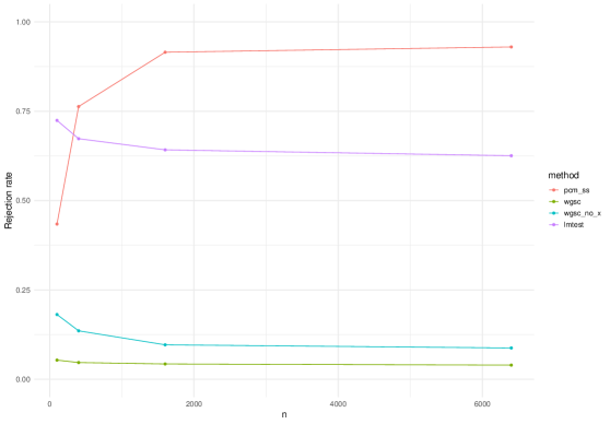
Figure S1: Power in the alternative settings considered in Section S6.1 for nominal 5%-level tests.

S6.2 Generalised additive models with binary responses

Here we consider settings similar to those considered in Section 6.1, but with $Y$ binary. Our null settings use

$${\mathbb{P}}(Y=1)=\mathrm{logit}(\sin(2\pi Z_{1})),$$

and we consider three alternative settings mirroring those in Section 6.1:

1. ${\mathbb{P}}(Y=1)=\mathrm{logit}(\sin(2\pi Z_{1})+0.25X^{2})$,

2. ${\mathbb{P}}(Y=1)=\mathrm{logit}(\sin(2\pi Z_{1})+0.5X^{2})$,

3. ${\mathbb{P}}(Y=1)=\mathrm{logit}(\sin(2\pi Z_{1})+0.5X^{2}Z_{2})$.

For all regressions with binary responses, we fit a binomial generalised additive model with logistic link, and we use additive models for all other regressions; we use the implementations in the R package mgcv (Wood,, 2017). The additive models are tuned as in Section 6.1 while the binomial additive models use half as many basis functions i.e. $\lfloor(N-1)/(2d)\rfloor$ (where $N$ and $d$ are the number of observations and predictors on which the model is trained, respectively) to avoid issues with convergence of the generalised additive model fits. The results can be seen in Figure S2 and are broadly in line with those in Section 6.1 with the PCM performing favourably though being powerless in Setting 3 with pure interactions (as to be expected), and wgsc and most notably gam not maintaining Type I error control.

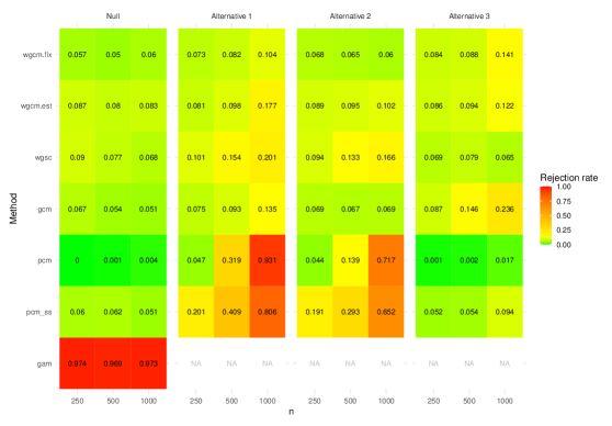
Figure S2: Rejection rates in the various settings considered in Section S6.2 for nominal 5%-level tests.

References

• Aït-Sahalia et al., (2001) Aït-Sahalia, Y., Bickel, P. J., and Stoker, T. M. (2001). Goodness-of-fit tests for kernel regression with an application to option implied volatilities. Journal of Econometrics, 105(2):363–412.
• Arias-Castro et al., (2018) Arias-Castro, E., Pelletier, B., and Saligrama, V. (2018). Remember the curse of dimensionality: The case of goodness-of-fit testing in arbitrary dimension. Journal of Nonparametric Statistics, 30(2):448–471.
• Belloni et al., (2015) Belloni, A., Chernozhukov, V., Chetverikov, D., and Kato, K. (2015). Some new asymptotic theory for least squares series: Pointwise and uniform results. Journal of Econometrics, 186(2):345–366.
• Belloni et al., (2011) Belloni, A., Chernozhukov, V., and Wang, L. (2011). Square-root lasso: pivotal recovery of sparse signals via conic programming. Biometrika, 98(4):791–806.
• Bengs and Holzmann, (2019) Bengs, V. and Holzmann, H. (2019). Uniform approximation in classical weak convergence theory. arXiv preprint arXiv:1903.09864.
• Berrett et al., (2020) Berrett, T. B., Wang, Y., Barber, R. F., and Samworth, R. J. (2020). The conditional permutation test for independence while controlling for confounders. Journal of the Royal Statistical Society: Series B (Statistical Methodology), 82(1):175–197.
• Bojer and Meldgaard, (2021) Bojer, C. S. and Meldgaard, J. P. (2021). Kaggle forecasting competitions: An overlooked learning opportunity. International Journal of Forecasting, 37(2):587–603.
• Breiman, (2001) Breiman, L. (2001). Random forests. Machine Learning, 45(1):5–32.
• Bühlmann and van de Geer, (2011) Bühlmann, P. and van de Geer, S. (2011). Statistics for High-Dimensional Data: Methods, Theory and Applications. Springer Publishing Company, Incorporated, 1st edition.
• Cai et al., (2022) Cai, Z., Lei, J., and Roeder, K. (2022). Model-free prediction test with application to genomics data. Proceedings of the National Academy of Sciences, 119(34).
• Candès et al., (2018) Candès, E., Fan, Y., Janson, L., and Lv, J. (2018). Panning for gold: ‘model-X’ knockoffs for high dimensional controlled variable selection. Journal of the Royal Statistical Society: Series B (Statistical Methodology), 80(3):551–577.
• Chernozhukov et al., (2018) Chernozhukov, V., Chetverikov, D., Demirer, M., Duflo, E., Hansen, C., Newey, W., and Robins, J. (2018). Double/debiased machine learning for treatment and structural parameters. The Econometrics Journal, 21(1).
• Cox, (1975) Cox, D. R. (1975). A note on data-splitting for the evaluation of significance levels. Biometrika, 62(2):441–444.
• Dai et al., (2022) Dai, B., Shen, X., and Pan, W. (2022+). Significance tests of feature relevance for a blackbox learner. IEEE Transactions on Neural Networks and Learning Systems, to appear.
• de Boor, (1976) de Boor, C. (1976). Splines as linear combinations of b-splines. a survey.
• DiCiccio et al., (2020) DiCiccio, C. J., DiCiccio, T. J., and Romano, J. P. (2020). Exact tests via multiple data splitting. Statistics & Probability Letters, 166:108865.
• Durrett, (2019) Durrett, R. (2019). Probability: Theory and Examples. Cambridge Series in Statistical and Probabilistic Mathematics. Cambridge University Press, 5th edition.
• Fan and Li, (1996) Fan, Y. and Li, Q. (1996). Consistent model specification tests: omitted variables and semiparametric functional forms. Econometrica, 64(4):865–890.
• Fernández and Rivera, (2022) Fernández, T. and Rivera, N. (2022). A general framework for the analysis of kernel-based tests. arXiv preprint arXiv:2209.00124.
• Goodfellow et al., (2016) Goodfellow, I., Bengio, Y., and Courville, A. (2016). Deep Learning. MIT press.
• Guo and Shah, (2023) Guo, F. R. and Shah, R. D. (2023). Rank-transformed subsampling: inference for multiple data splitting and exchangeable p-values. arXiv preprint arXiv:2301.02739.
• Gut, (2013) Gut, A. (2013). Probability: A Graduate Course. Springer New York.
• Györfi et al., (2002) Györfi, L., Kohler, M., Krzyzak, A., and Walk, H. (2002). A distribution-free theory of nonparametric regression. Springer.
• Heinze-Deml et al., (2018) Heinze-Deml, C., Peters, J., and Meinshausen, N. (2018). Invariant causal prediction for nonlinear models. Journal of Causal Inference, 6(2):20170016.
• Huang, (2003) Huang, J. Z. (2003). Local asymptotics for polynomial spline regression. The Annals of Statistics, 31(5):1600 – 1635.
• Ichimura and Newey, (2015) Ichimura, H. and Newey, W. K. (2015). The influence function of semiparametric estimators. arXiv preprint arXiv:1508.01378.
• Ingster, (1987) Ingster, Y. I. (1987). Minimax testing of nonparametric hypotheses on a distribution density in the $L_{p}$ metrics. Theory of Probability & Its Applications, 31(2):333–337.
• Ingster, (2000) Ingster, Y. I. (2000). Adaptive chi-square tests. Journal of Mathematical Sciences, 99(2):1110–1119.
• Janková et al., (2020) Janková, J., Shah, R. D., Bühlmann, P., and Samworth, R. J. (2020). Goodness-of-fit testing in high dimensional generalized linear models. Journal of the Royal Statistical Society: Series B (Statistical Methodology), 82(3):773–795.
• Jin et al., (2018) Jin, Z., Yan, X., and Matteson, D. S. (2018). Testing for conditional mean independence with covariates through martingale difference divergence. In Proceedings of the Thirty-Fourth Conference on Uncertainty in Artificial Intelligence, UAI 2018, Monterey, California, USA, August 6-10, 2018, pages 1–12. AUAI Press.
• Kasy, (2019) Kasy, M. (2019). Uniformity and the delta method. Journal of Econometric Methods, 8(1).
• Kennedy, (2020) Kennedy, E. H. (2020). Optimal doubly robust estimation of heterogeneous causal effects. arXiv preprint arXiv:2004.14497.
• Kim and Ramdas, (2023) Kim, I. and Ramdas, A. (2023+). Dimension-agnostic inference using cross $U$-statistics. Bernoulli, to appear.
• Klenke, (2020) Klenke, A. (2020). Probability Theory. Springer International Publishing.
• Lavergne and Vuong, (2000) Lavergne, P. and Vuong, Q. (2000). Nonparametric significance testing. Econometric Theory, 16(4):576–601.
• Lepskiǐ, (1991) Lepskiǐ, O. V. (1991). Asymptotically minimax adaptive estimation i: Upper bounds. optimally adaptive estimates. Theory Probab. Appl., 36:682–697.
• Lovász and Vempala, (2007) Lovász, L. and Vempala, S. (2007). The geometry of logconcave functions and sampling algorithms. Random Structures & Algorithms, 30(3):307–358.
• Lundborg et al., (2022) Lundborg, A. R., Shah, R. D., and Peters, J. (2022). Conditional independence testing in Hilbert spaces with applications to functional data analysis. Journal of the Royal Statistical Society: Series B (Statistical Methodology), 84(5):1821–1850.
• Meinshausen and Bühlmann, (2010) Meinshausen, N. and Bühlmann, P. (2010). Stability selection. Journal of the Royal Statistical Society: Series B (Statistical Methodology), 72(4):417–473.
• Meinshausen et al., (2009) Meinshausen, N., Meier, L., and Bühlmann, P. (2009). P-values for high-dimensional regression. Journal of the American Statistical Association, 104(488):1671–1681.
• Mendelson and Zhivotovskiy, (2020) Mendelson, S. and Zhivotovskiy, N. (2020). Robust covariance estimation under $L_{4}-L_{2}$ norm equivalence. The Annals of Statistics, 48(3):1648–1664.
• Nemirovski, (2000) Nemirovski, A. (2000). Topics in non-parametric. Ecole d’Eté de Probabilités de Saint-Flour, 28:85.
• Newey and Robins, (2018) Newey, W. K. and Robins, J. R. (2018). Cross-fitting and fast remainder rates for semiparametric estimation. arXiv preprint arXiv:1801.09138.
• Neykov et al., (2021) Neykov, M., Balakrishnan, S., and Wasserman, L. (2021). Minimax optimal conditional independence testing. The Annals of Statistics, 49(4):2151–2177.
• Neyman, (1923) Neyman, J. (1923). Sur les applications de la théorie des probabilités aux experiences agricoles: Essai des principes. Roczniki Nauk Rolniczych, 10:1–51.
• Petersen and Hansen, (2021) Petersen, L. and Hansen, N. R. (2021). Testing conditional independence via quantile regression based partial copulas. Journal of Machine Learning Research, 22(70):1–47.
• Powell, (1981) Powell, M. J. D. (1981). Approximation Theory and Methods. Cambridge University Press.
• Rinaldo et al., (2019) Rinaldo, A., Wasserman, L., and G’Sell, M. (2019). Bootstrapping and sample splitting for high-dimensional, assumption-lean inference. The Annals of Statistics, 47(6):3438–3469.
• Romano, (2004) Romano, J. P. (2004). On Non-parametric Testing, the Uniform Behaviour of the $t$-test, and Related Problems. Scandinavian Journal of Statistics, 31(4):567–584.
• Rubin, (1974) Rubin, D. B. (1974). Estimating causal effects of treatments in randomized and nonrandomized studies. Journal of Educational Psychology, 66(5):688.
• Scheidegger et al., (2022) Scheidegger, C., Hörrmann, J., and Bühlmann, P. (2022). The Weighted Generalised Covariance Measure. Journal of Machine Learning Research, 23(1):12517–12584.
• Schumaker, (2007) Schumaker, L. (2007). Spline Functions: Basic Theory. Cambridge Mathematical Library. Cambridge University Press, 3 edition.
• Shah and Bühlmann, (2018) Shah, R. D. and Bühlmann, P. (2018). Goodness-of-fit tests for high dimensional linear models. Journal of the Royal Statistical Society: Series B (Statistical Methodology), 80(1):113–135.
• Shah and Peters, (2020) Shah, R. D. and Peters, J. (2020). The hardness of conditional independence testing and the generalised covariance measure. The Annals of Statistics, 48(3):1514–1538.
• Shah and Samworth, (2013) Shah, R. D. and Samworth, R. J. (2013). Variable selection with error control: another look at stability selection. Journal of the Royal Statistical Society: Series B (Statistical Methodology), 75(1):55–80.
• Shao and Zhang, (2014) Shao, X. and Zhang, J. (2014). Martingale difference correlation and its use in high-dimensional variable screening. Journal of the American Statistical Association, 109(507):1302–1318.
• Sun and Zhang, (2012) Sun, T. and Zhang, C.-H. (2012). Scaled sparse linear regression. Biometrika, 99(4):879–898.
• Tibshirani, (1996) Tibshirani, R. (1996). Regression shrinkage and selection via the lasso. Journal of the Royal Statistical Society: Series B (Methodological), 58(1):267–288.
• van der Vaart, (1998) van der Vaart, A. W. (1998). Asymptotic Statistics. Cambridge Series in Statistical and Probabilistic Mathematics. Cambridge University Press.
• Verdinelli and Wasserman, (2021) Verdinelli, I. and Wasserman, L. (2021). Decorrelated Variable Importance. arXiv preprint arXiv:2111.10853.
• Vovk and Wang, (2020) Vovk, V. and Wang, R. (2020). Combining $p$-values via averaging. Biometrika, 107(4):791–808.
• Wang and Samworth, (2018) Wang, T. and Samworth, R. J. (2018). High dimensional change point estimation via sparse projection. Journal of the Royal Statistical Society: Series B (Statistical Methodology), 80(1):57–83.
• Wang and Shah, (2020) Wang, Y. and Shah, R. D. (2020). Debiased Inverse Propensity Score Weighting for Estimation of Average Treatment Effects with High-Dimensional Confounders. arXiv preprint arXiv:2011.08661.
• Wasserman et al., (2020) Wasserman, L., Ramdas, A., and Balakrishnan, S. (2020). Universal inference. Proceedings of the National Academy of Sciences, 117(29):16880–16890.
• Wasserman and Roeder, (2009) Wasserman, L. and Roeder, K. (2009). High dimensional variable selection. The Annals of Statistics, 37(5A):2178–2201.
• White, (1980) White, H. (1980). A heteroskedasticity-consistent covariance matrix estimator and a direct test for heteroskedasticity. Econometrica, 48(4):817–838.
• Williamson et al., (2021) Williamson, B. D., Gilbert, P. B., Carone, M., and Simon, N. (2021). Nonparametric variable importance assessment using machine learning techniques. Biometrics, 77:9–22.
• Williamson et al., (2022) Williamson, B. D., Gilbert, P. B., Simon, N. R., and Carone, M. (2022+). A general framework for inference on algorithm-agnostic variable importance. Journal of the American Statistical Association, to appear.
• Wood, (2013) Wood, S. N. (2013). On p-values for smooth components of an extended generalized additive model. Biometrika, 100(1):221–228.
• Wood, (2017) Wood, S. N. (2017). Generalized Additive Models. Chapman and Hall/CRC.
• Wright and Ziegler, (2017) Wright, M. N. and Ziegler, A. (2017). ranger: A fast implementation of random forests for high dimensional data in C++ and R. Journal of Statistical Software, 77(1):1–17.
• Zeileis and Hothorn, (2002) Zeileis, A. and Hothorn, T. (2002). Diagnostic checking in regression relationships. R News, 2(3):7–10.
• Zhang et al., (2011) Zhang, K., Peters, J., Janzing, D., and Schölkopf, B. (2011). Kernel-Based Conditional Independence Test and Application in Causal Discovery. In Proceedings of the Twenty-Seventh Conference on Uncertainty in Artificial Intelligence, UAI’11, pages 804–813, Arlington, Virginia, USA. AUAI Press.
• Zhang and Janson, (2020) Zhang, L. and Janson, L. (2020). Floodgate: inference for model-free variable importance. arXiv preprint arXiv:2007.01283.
\appendixpage