Constant-overhead Differentially Private Hyperparameter Tuning

Abstract

Hyperparameter tuning is a ubiquitous procedure in machine learning, but it has often been entirely ignored in the literature on privacy-preserving machine learning, partly due to its negative impact on privacy loss parameter. In this paper, we aim to tackle this problem by developing a differentially private hyperparameter tuning framework with constant overhead on the privacy parameter. One relevance of our results is that we are allowed to expand the hyperparameter search space (even adopt a grid search) without worrying about the potential increase in privacy leakage, since additional privacy loss parameter is independent of the number of hyperparameter candidates and the original privacy parameter for a single run. Our theoretical analysis shows that the additional privacy loss incurred by hyperparameter tuning is upper-bounded by the logarithm of the utility term. Moreover, our proposed method is compatible with adaptive hyperparameter optimization methods, which can be used for efficiency improvement.

Table 1: Comprehensive comparison between different methods for hyperparameter tuning with differential privacy.

Method	Grid search	Adaptive optimization	Private train per search	Privacy budget
Naive	Support	Compatible	Required	$\tilde{O}(|\mathcal{S}|^{0.5}\varepsilon$)
RandTuneLiu and Talwar (2019); Papernot and Steinke (2022)	N/A	Incompatible	Required	$2\varepsilon$ or $3\varepsilon$
Ours	Support	Compatible	Optional	$\varepsilon+O(\log{\frac{u^{*}-u_{0}}{g}})\epsilon$

1 Introduction

Differential privacy Dwork et al. (2006, 2014) has been the gold standard for quantitative and rigorous reasoning about privacy leakage from the processing of private data. Applying differential privacy to machine learning Song et al. (2013); Bassily et al. (2014); Abadi et al. (2016) is a long-lasting challenge due to the dramatic reduction in the model utility compared with the non-private version Tramèr and Boneh (2021). This motivates a bunch of work dedicated to designing private learning algorithms without sacrificing utility Sajadmanesh and Gatica-Perez (2021); Kolluri et al. (2022). However, researchers typically try different hyperparameters for best possible performance but only report the privacy parameter of a single run, which corresponds to the best accuracy achieved. As shown in Papernot and Steinke (2022), the choice of hyperparameter would cause leakage of private information such as membership inference Shokri et al. (2017). This finding is aligned with the theory of differential privacy if applied strictly. Supposed one run of private learning to be $\varepsilon$-DP, if we repeat the learning process $K$ times using different hyperparameters and select the model with the highest accuracy, the privacy loss parameter would be increased to $O(k\varepsilon)$ with basic composition or $\tilde{O}(\sqrt{k}\varepsilon)$ with advanced composition Dwork et al. (2010); Kairouz et al. (2015), essentially a multiple of the original privacy loss $\varepsilon$. Several existing works attempt to handle such embarrassment. The stability-based approach Chaudhuri and Vinterbo (2013) leverages the stability assumption of the learning algorithm for improving the privacy loss bounds. RandTune Liu and Talwar (2019); Papernot and Steinke (2022) proposes to introduce another level of uncertainty for sharpening the privacy bounds. Concretely, it first draws $K$ from a geometric distribution, then randomly and independently picks $K$ hyperparameters, and runs a private training algorithm for each selected hyperparameter. Then the total privacy parameter is shown to be bounded by 2 or 3 times of the privacy parameter for a single run. However, the largest challenge in RandTune is to guarantee the success probability of picking the best hyperparameter within only $K$ independent trials, which gets more difficult when the search space of hyperparameters is large. Therefore, a recent work Mohapatra et al. (2022) leverages adaptive optimizers to reduce the potential hyperparameter space. Nevertheless, the number of trials remains to be unpredictable, and therefore it is intrinsically hard to guarantee the model quality.

In this paper, we propose a constant-overhead differentially private hyperparameter tuning framework, which rigorously satisfies the guarantees of differential privacy for the entire pipeline of machine learning, including private training and hyperparameter tuning. By constant overhead, we mean that 1) the additional privacy parameter due to hyperparameter tuning is independent of the original privacy parameter of private training for a single run, i.e., a constant with respect to $\varepsilon$, and 2) the overhead is independent of hyperparameter space, i.e., a constant with respect to $|\mathcal{S}|$. The direct implication is that we are free to adopt a significantly larger hyperparameter search space, e.g. grid search, to seek the best possible hyperparameter configuration, and thus the best possible model parameter. One interesting property of our method is that the overhead now correlates with the final utility of the model (i.e., accuracy on the validation set), which passes a sanity check because it explicitly reveals the trade-off between privacy and utility. Additionally, our approach does not require each training run for hyperparameter selection to be differentially private. Therefore, it has the potential to significantly boost computational efficiency for hyperparameter tuning considering the computational cost of private training is much larger than that of non-private training due to the calculation of the per-sample gradient Tramer and Boneh (2020); Lee and Kifer (2021). It is worth noting that our method is compatible with adaptive hyperparameter optimization methods Mockus et al. (1978); Swersky et al. (2013), a powerful tool for tuning the hyperparameters with efficiency. We defer the discussion of adaptive optimization to Section 4. Comparisons between different methods are shown in Table 1.

To conclude, our contribution is listed as follows.

• We propose a randomized algorithm that achieves differentially private hyperparameter tuning within constant privacy overhead, which will hopefully help tackle this fundamental yet relevant problem in the application of privacy-preserving machine learning.

• We present a comprehensive theoretical analysis of the proposed algorithm, showing that the overhead is the logarithm of the utility term, a significant improvement over the trivial result of polynomial dependence.

Table 2: Some notations and their explanations.

Notation	Explanation
$\varepsilon$, $\epsilon$, $\delta$	Privacy parameter
$\mathcal{S}$	Set of hyperparameter candidates
$\dot{u}_{\cdot}^{\cdot}\in[0,1]$	Some utility score
$u_{0}$	Initial value of $u$ in Algorithm 1
$u_{s},s\in[|\mathcal{S}|]$	Utility score of each hyperparameter
$u^{*}$	Threshold of utility check
$\hat{u}$	Maximum of $u_{s},s\in[|\mathcal{S}|]$
$s^{*}\in[|\mathcal{S}|]$	Index of $u^{*}$ into $\mathcal{S}$
$g\in(0,1)$	Utility granularity
$step\in\mathbb{N}$	Step size for utility accumulation
$T\in\mathbb{Z}^{+}$	Number of iterations in Algorithm 1
$k\in\mathbb{Z}^{+}$	Number of partitions of $D_{train}$
$n$	Shorthand notation of $(u^{*}-u_{0})/g$
$\theta$	ML model parameter (after training)

2 Background

Differential privacy Dwork et al. (2006) basically requires that the distribution of an algorithm’s output is nearly indistinguishable from the output obtained under small perturbations of its input. The formal definition is given as follows.

Definition 1.

$\varepsilon$-Differential Privacy: A randomized mechanism $\mathcal{M}:\mathcal{D}\rightarrow\mathcal{R}$ satisfies $\varepsilon$-differential privacy if for any two adjacent datasets $\mathcal{D},\mathcal{D}^{\prime}\in{\rm Domain}(\mathcal{M})$ and for all $S\in{\rm Range(\mathcal{M})}$ it holds that

$$\operatorname{Pr}(\mathcal{M}(\mathcal{D})\in\mathcal{S}))\leq e^{\varepsilon}\operatorname{Pr}\left(\mathcal{M}(\mathcal{D}^{\prime})\in\mathcal{S})\right)$$ (1)

$\varepsilon$-DP is also known as pure DP, which says that privacy loss parameter $\ln\operatorname{Pr}(\mathcal{M}(\mathcal{D})\in\mathcal{S}))/\operatorname{Pr}\left(\mathcal{M}(\mathcal{D}^{\prime})\in\mathcal{S})\right)$ is bounded by $\varepsilon$ with possibility of 1. If tiny failure rate $\delta$ is allowed, we have the following definition of $(\varepsilon,\delta)$-DP, also called approximate DP.

Definition 2.

$(\varepsilon,\delta)$-Differential Privacy: A randomized mechanism $\mathcal{M}:\mathcal{D}\rightarrow\mathcal{R}$ satisfies $(\varepsilon,\delta)$-differential privacy if for any two adjacent datasets $\mathcal{D},\mathcal{D}^{\prime}\in{\rm Domain}(\mathcal{M})$ and for all $S\in{\rm Range(\mathcal{M})}$ it holds that

$$\operatorname{Pr}(\mathcal{M}(\mathcal{D})\in\mathcal{S}))\leq e^{\varepsilon}\operatorname{Pr}\left(\mathcal{M}(\mathcal{D}^{\prime})\in\mathcal{S})\right)+\delta$$ (2)

In the following, we introduce one basic differential private algorithm, Laplace mechanism. Before that, we first give the definition of $\ell_{1}$ sensitivity of a function.

Definition 3.

$\ell_{1}$ Sensitivity: Let $f$: $\mathcal{D}^{n}\rightarrow R^{k}$. The $\ell_{1}$ sensitivity of $f$ is

$$\Delta^{(f)}=\operatorname{max}_{\mathcal{D},\mathcal{D}^{\prime}}\|f(\mathcal{D})-f(\mathcal{D}^{\prime})\|_{1}$$ (3)

where $D$ and $D^{\prime}$ are neighbouring datasets.

Note that $\ell_{1}$ sensitivity is the intrinsic property of one function, which does not depend on the distribution of dataset. Thus it is sometimes referred to as global $\ell_{1}$ sensitivity.

Definition 4.

Laplace mechanism: Let $f$: $\mathcal{D}^{n}\rightarrow R^{k}$. The Laplace mechanism is defined as

$$\mathcal{\mathcal{D}}=f(\mathcal{D})+\operatorname{Lap}\left(\frac{\Delta^{(f)}}{\varepsilon}\right)$$ (4)

where $\operatorname{Lap}\left(\frac{\Delta^{(f)}}{\varepsilon}\right)$ is sampled from Laplace distribution $\operatorname{Lap}(x;b)=\textnormal{exp}(-|x|/b)$ with parameter $b=\frac{\Delta^{(f)}}{\varepsilon}$. Laplace mechanism is $\varepsilon$-DP.

Finally, we introduce one nice property of differential privacy, composability, which states that for a series of steps, if each of which is differentially private, the overall privacy parameter of the entire process is the sum of the individual privacy parameter of each step.

Theorem 1.

(Composition theorem). If a mechanism $M$ consists of a sequence of adaptive mechanisms $M_{1},...,M_{k}$ such that for any $i\in[k]$, $M_{i}$ guarantees $(\varepsilon_{i},\delta_{i})$-DP, then $M$ guarantees $(\sum_{i=1}^{k}\varepsilon_{i},\sum_{i=1}^{k}\delta_{i})$-DP.

This theorem allows for the composition of multiple differentially private mechanisms to be used in a pipeline, while still providing a strong privacy guarantee.

Algorithm 1 Constant-overhead Differentially Private Hyperparameter Tuning

Input: Set of hyperparameter candidates $\mathcal{S}$; Training set $\mathcal{D}_{train}$; Validation set $\mathcal{D}_{valid}$; Utility lower bound $u_{0}\in[0,1)$.
Parameter: Privacy parameters $\varepsilon,\epsilon>0,\delta\in(0,1)$; Number of partitions $k$; Utility granularity $g\in(0,1)$;
Output: Model parameters $\theta^{*}$ along with the selected hyperparameters $s^{*}\in\mathcal{S}$.

1:Partition the training set $\mathcal{D}_{train}$ into disjoint subsets $\mathcal{D}_{i}$, $i=1,2,...,k$;

2:for s = $1,2,...,|\mathcal{S}|$ do

3:     Initialize $u_{s}\leftarrow 0$;

4:     for $i$ = $1,2,...,k$ do

5:         $\theta\leftarrow{{\rm Train}}(\mathcal{D}_{i},\mathcal{S}_{s})$ or ${{\rm PrivTrain}}(\mathcal{D}_{i},\mathcal{S}_{s},\varepsilon,\delta)$;

6:         $u_{s}^{(i)}\leftarrow{{\rm Acc}}(\mathcal{D}_{valid},\theta)$

7:$\triangleright$ Compute utility for each partition

8:     end for

9:     $u_{s}\leftarrow\frac{1}{k}\sum_{i=1}^{k}u_{s}^{(i)}$

10:$\triangleright$ Compute average utility across partitions

11:end for

12:Initialize $s^{*}\leftarrow\emptyset$, $u\leftarrow u_{0}$, $step\leftarrow 1$;

13:Initialize $T\leftarrow 0$ $\triangleright$ Help variable for algorithmic analysis

14:while $step\neq 0$ do

15:     $T\leftarrow T+1$

16:     Let $\hat{u}\leftarrow u+step\times g+{{\rm Lap}}(2/(k\epsilon))$

17:$\triangleright$ Propose a utility threshold

18:     $isAccumulated\leftarrow\textbf{False}$;

19:     for s = $1,2,...,|\mathcal{S}|$ do

20:         $\gamma_{s}\leftarrow{{\rm Lap(4}}/(k\epsilon))$ $\triangleright$ Sample noise

21:         if $u_{s}+\gamma_{s}\geq\hat{u}$ then

22:              $s^{*}\leftarrow s$ $\triangleright$ Record the current hyperparameter

23:              $u\leftarrow u+g\cdot step$ $\triangleright$ Accumulate utility

24:              $isAccumulated\leftarrow\textbf{True}$;

25:              $step\leftarrow 2\cdot step$

26:$\triangleright$ Elastic increase of the step size

27:              break;

28:         end if

29:     end for

30:     if not $isAccumulated$ then

31:         $step\leftarrow\lfloor step/2\rfloor$

32:$\triangleright$ Elastic decrease of the step size

33:     end if

34:end while

35:return $\theta^{*}\leftarrow{{\rm PrivateTrain}}(\mathcal{D}_{train},S_{s^{*}},\varepsilon,\delta)$

36:$\triangleright$ Using the selected hyperparameter

3 Constant-overhead Differentially Private Hyperparameter Tuning

Our method shown in Algorithm 1 is inspired by a bunch of classical algorithms. Specifically, we inherit the AboveThreshold component (line 18) of Sparse Vector Technique Dwork et al. (2009) to check whether the current candidate is eligible for utility accumulation. We also apply Subsample and Aggregate Nissim et al. (2007) (lines 3-11) to help us obtain a proxy utility function with relatively low sensitivity (also used by PATE Papernot et al. (2017, 2018)). The key algorithmic novelty and the main technique contribution is the design of elastically geometrical increase and decrease of the utility accumulation step, which is inspired by the doubling algorithm for solving Lowest-Common-Ancestor (LCA) in the tree. We make non-trivial modifications to accommodate the probabilistic nature of differential privacy, which unfortunately makes the algorithmic analysis significantly more complicated. In this section, after description of the algorithm, we will provide theoretical analysis showing that the privacy overhead incurred by hyperparameter tuning is upper-bounded by the logarithm of the gained utility.

3.1 Algorithm Description

The full description is shown in Algorithm 1. We first implement the function of $\textnormal{Eval}(\mathcal{D}_{valid},S_{s};\mathcal{D}_{train})$ given the training dataset, and validation dataset for all hyperparameter configuration $S_{s}$ (line 1-11). This functionality is realized with small sensitivity with respect to $\mathcal{D}_{train}$ by first partitioning $\mathcal{D}_{train}$ into $k$ disjoint subsets, on which we separately train $k$ models. After that, the utility for the current hyperparameter is obtained by taking the average accuracy over all $k$ models. Then we enter into a series of iterations. In each iteration, we start with some utility threshold, which takes the current utility (initialized as $u_{0}$) and adds it by the current step size with calibrated noise. We then check whether there exists a hyperparameter configuration whose utility exceeds that threshold after injecting noise. Once the threshold check is satisfied, we accumulate the utility by the step size, geometrically increase the step size, and directly enter into the next iteration. If it turns out that none of the hyperparameters passes it, we geometrically decrease the step size and enter into the next iteration. Intuitively, the larger the utility some hyperparameter has, the more likely it leads to a utility accumulation. Figure 1 visually illustrates the elastic dynamics of the step size and the evolvement of the utility as iteration goes by.

3.2 Algorithm Analysis

In this section, we provide a thorough analysis of our proposed algorithm, which basically consists of two lines. One line is to bound the total iterations needed for the algorithm to terminate. Another line is to track the privacy loss of the whole process. We start by some lemmas, followed by the two main theorems of this paper.

To facilitate the proof of the main results of this work as well as provide some basic intuition behind them, we will first study the dual results in the non-randomized world. The definition of the non-randomized world is as follows.

Definition 5.

Non-randomized World. In the non-randomized world, all the noise in Algorithm 1 will be zero.

It turns out that it is much more straightforward to analyze Algorithm 1 in the non-randomized world. We have the following lemma.

Figure 1: 2D visulaization of Algorithm 1 over iterations. The algorithm begins with $u=u_{0}$ and $step=1$. The top red bar (slightly shifted above) corresponds to the bound in Equation (11).

Lemma 1.

In the non-randomized world, $u$ will arrive at $u^{*}$ after $T=O(\log\frac{u^{*}-u_{0}}{g})$ iterations.

Proof.

Let $n=\lceil\frac{u^{*}-u_{0}}{g}\rceil$. We first consider a special case where $n=2^{k}-1$ for some integer $k$. Note that $\sum_{i=1}^{k}2^{i}\cdot g$ = $(2^{k}-1)g=ng\geq u^{*}-u_{0}$. It takes $k=O(\log\frac{u^{*}-u_{0}}{g})$ iterations for $u$ to arrive at $u^{*}$.

If $n=2^{k}-1+n^{\prime}$ where $n^{\prime}\in[1,2^{k})$, it first takes $k=O(\log\frac{u^{*}-u_{0}}{g})$ iterations for $u$ to arrive at $2^{k}-1$. At that time, $step=2^{k}$, we have $u+step\cdot g=u_{0}+g(2^{k}-1)+2^{k}\cdot g>u_{0}+g(2^{k}-1)+n^{\prime}\cdot g>u^{*}$. Thus, the threshold test will not be passed, and the value of $step$ will begin to geometrically decrease in the following iteration(s). To help analysis, we represent $n^{\prime}$ in base 2, $n^{\prime}=2^{j_{1}}+2^{j_{2}}+...+2^{j_{m}}$, where $j_{1}>j_{2}>j_{m}$. During the process of $step$ decreasing to 0, each time when $step=2^{j_{i}}$, it will successfully pass the check, and $step$ will be doubled to become $2^{j_{i}+1}$. In the next iteration, the check will not be passed, and $step$ will decrease to $2^{j_{i}}$. After that, $step$ continue to decrease and repeat this pattern until termination. Therefore, it takes $2m+k$ iterations for $step$ to return to 0, thus $2m+2k$ iterations overall. Note that $m=O(\log n^{\prime})=O(\log n)$. It takes $2m+2k=O(\log\frac{u^{*}-u_{0}}{g})$ iterations for $u$ to arrive at $u^{*}$. ∎

From Lemma 1, intuition would suggest that it would roughly takes $O(\log\frac{u^{*}-u_{0}}{g})$ iterations for Algorithm 1 to terminate in the randomized world. We formally prove it as our first main result as follows, which is technically much more challenging than above.

Theorem 2.

(main results) With high possibility, $T$ in Algorithm 1 (line 13) is bounded by $O(\log\frac{u^{*}-u_{0}}{g})$.

Proof.

For simplicity, we will denote $n=\frac{u^{*}-u_{0}}{g}$. We can observe that $u$ in Algorithm 1 (line 20) is monotonically non-decreasing. Thus we can split the whole execution into two phases as follows: $u\leq u^{*}-g\log\frac{u^{*}-u_{0}}{g}$ corresponds to the grow phase and $u>u^{*}-g\log\frac{u^{*}-u_{0}}{g}$ corresponds to the convergence phase. In the remaining part of the proof, we bound the iterations in each phase separately.

I. Bounded iterations during the grow phase.

We begin by considering the the probability of the variable $isAccumulated$ in Algorithm 1 (line 15) is False when $\hat{u}\leq u^{*}-g\log n$. Note that this may not always hold true during the grow phase.

$$\begin{split}&\Pr[isAccumulated=\textnormal{False}~{}|~{}\hat{u}\leq u^{*}-g\log n]\\ =&\Pr[\bigcap_{s\in[|\mathcal{S}|]}\gamma_{s}<\hat{u}-u_{s}~{}|~{}\hat{u}\leq u^{*}-g\log n]\\ \leq&\Pr[\gamma_{s^{*}}<\hat{u}-u_{s^{*}}~{}|~{}\hat{u}\leq u^{*}-g\log n]\\ \leq&\Pr[\gamma_{s^{*}}>|\hat{u}-u_{s^{*}}|~{}|~{}|\hat{u}-u_{s^{*}}|\geq g\log n]\\ \leq&{{\rm exp}}(-(gk\epsilon\log n)/4))\leq n^{-gk\epsilon/4}\\ \end{split}$$ (5)

where the first inequality is due to $\Pr[A\cap B]\leq\Pr[A])$, and the third inequality is the tail bound for Laplace distribution. Similarly, we have the following symmetric inequality, which will be used later in part II.

$$\Pr[isAccumulated=True~{}|~{}\hat{u}\geq u^{*}+\log n]\leq n^{-k\epsilon/4}$$ (6)

(i) If $|\hat{u}-u^{*}|\geq g\log\frac{u^{*}-u_{0}}{g}$ throughout grow phase.

We claim that in this case the behavior of $u$ in the first $O(\log n)$ iterations in the randomized world is identical to the non-randomized world with high possibility. Indeed, denote $X_{i}$ as the random variable that equals True when the behavior of $u$ is identical across randomized and non-randomized world at iteration $i$, then the probability of the identical behavior within $T_{g}$ iterations is as follows,

$$\begin{split}&\Pr[X_{1}\cap X_{2}\cap X_{3}\cap...\cap X_{T_{g}}]\\ =&\Pr[X_{1}]\cdot\Pr[X_{2}|X_{1}]\cdot...\cdot\Pr[X_{T_{g}}|X_{1}\cap X_{2}\cap..\cap X_{T_{g}-1}]\\ \end{split}$$ (7)

Note that $X_{i}|X_{1}\cap...\cap X_{i-1}$ holds true if and only if $isAccumulated=\mathbb{I}[\hat{u}\leq u^{*}]$ in the randomized world. We can then bound each probability term using Equation (5) by

$$\begin{split}&\Pr[X_{i}|X_{1}\cap X_{2}\cap...\cap X_{i-1}]\\ =&\Pr[isAccumulated=\textnormal{True}~{}|~{}\hat{u}\leq u^{*}-g\log n]\\ \geq&(1-n^{-gk\epsilon/4})\geq{{\rm exp}}(n^{-gk\epsilon/4}+O(n^{-gk\epsilon/2}))\end{split}$$ (8)

The last inequality uses the fact that $1-x\geq\textnormal{exp}(-x-C\cdot x^{2})$ for some $C>0$ when $x\in(0,1)$. If we choose $T_{g}$ to be $O(\log n)$, we have

$$\begin{split}(\ref{eq:same})&\geq{{\rm exp}}(n^{-gk\epsilon/4}+O(n^{-gk\epsilon/2}))^{T_{g}}\\ &\geq{{\rm exp}}(O(n^{-gk\epsilon/4}\log n+n^{-gk\epsilon/2}\log n)\\ &\geq 1-O(n^{-gk\epsilon/4}\log n)=1-o(1)\end{split}$$ (9)

which states that in this case the behavior of $u$ is identical to the non-randomized world with high possibility, as long as the concerned iterations is bounde by $O(\log n)$. Then we can prove by contradiction. Suppose that after $T_{g}=O(\log n)$ iterations, the execution still stays in the grow phase, i.e., $u<u^{*}-g\log n$. By Lemma 1, we know that $u$ will be equal to $u^{*}$ in $O(\log n)$ iterations if its behavior is identical to the non-randomized world. which leads to contradiction. Hence, the grow phase will have at most $T_{g}=O(\log n)$ iterations, after which $u$ is at least $u^{*}-g\log n$.

(ii) Otherwise.

We then consider the situation where $|\hat{u}-u^{*}|>g\log n$ does not always hold true during the grow phase. Suppose this condition is violated at iteration $j$, there are two cases:

(a) If $X_{j}|X_{1}\cap...\cap X_{j-1}$ holds true, which is desirable since its behavior remains the same as that in the non-randomized world. We can then use the similar reasoning as in (i) to bound the number of iterations.

(b) If $X_{j}|X_{1}\cap...\cap X_{j-1}$ is false, which means that we are deviated from the non-randomized world, that is, $isAccumulated=\mathbb{I}[\hat{u}>u^{*}]$.

(b.i) If $u^{*}\leq\hat{u}<u^{*}+g\log n$ at iteration $j$, which means $Accumulated=\textnormal{True}$ and $\hat{u}>u^{*}$. Note that the grow phase will end immediately after this iteration since the threshold check is already passed and $u$ will be increased to be larger than $u^{*}-g\log n$. Hence the grow phase will also have at most $O(\log n)$ iterations.

(b.ii) If $u^{*}-g\log n<\hat{u}<u^{*}$ at iteration $j$. Note that at that time we have $Accumulated=\textnormal{False}$ when $u^{*}-g\log n\leq\hat{u}<u^{*}$. Recall that from Equation (5) we also have $Accumulated=\textnormal{True}$ when $\hat{u}\leq u^{*}-g\log n$. Therefore, the following relation will hold true.

$$isAccumulated=\mathbb{I}[\hat{u}\leq u^{*}-g\log n]$$ (10)

which is equivalent to the non-randomized world with the parameter $u^{*}\leftarrow u^{*}-g\log n$. We know from Lemma 1 that it will take $T=O(\log\frac{u^{*}-g\log n-u_{0}}{g})=O(\log n-\log\log n)=O(\log n)$ to arrive at $u^{*}-g\log n$. Hence the grow phase will also have at most $O(\log n)$ iterations.

II. Bounded iterations during the convergence phase.

We now prove that it takes $O(\log n)$ for Algorithm 1 to terminate once $u>u-\log n$. We begin by bounding the value of $step$ at the first iteration of the convergence phase, denoted by $step_{c}$. Then we bound the number of times when $isAccumulated=\textnormal{True}$ during the convergence phase, denoted by, $A_{c}$. Finally, we are able to bound the number of iterations during the convergence phase, denoted by $T_{c}$.

(i) Bounding $step_{c}$.

We claim that $step\leq\frac{u-u_{0}}{g}+1$ holds true for all iterations and prove it via induction. At iteration 1, $step=1$, $u=u_{0}$, thus the inequality holds true. Suppose it holds true for iteration $k$, we have $step_{k}\leq u_{k}+1$. For iteration $k+1$, if $isAccumulated$ is false, $step_{k+1}<=step_{k}/2$ and $u_{k}=u_{k+1}$. Otherwise, $u_{k+1}=u_{k}+g\cdot step_{k}$ and $step_{k+1}=step_{k}*2$. Either case we still have $step_{k+1}\leq\frac{u_{k+1}-u_{0}}{g}+1$. Denote $step_{c^{-}}$ (or $u_{c^{-}}$) as the value of $step$ (or $u$) at the last iteration of the grow phase. Therefore, we have

$$step_{c}=2\cdot step_{c^{-}}\leq 2\left(\frac{u_{c^{-}}-u_{0}}{g}+1\right)\leq 2(n+1)$$ (11)

(ii) Bounding $A_{c}$.

Following the similar reasoning in Equations (5)-(9), $u$ will be less than $u^{*}+g\log n$ within $O(\log n)$ iterations with high possibility. Then we have

$$\begin{split}u^{*}+g\log n&\geq u_{c}+\sum_{i=T_{g}+1}^{T_{g}+T_{c}}{step_{i}\cdot\mathbb{I}[isAccumulated_{i}]}\\ &\geq u^{*}-g\log n+A_{c}*1\end{split}$$ (12)

The second inequality holds because there are $A_{c}$ terms contributing to the summation and each $step_{i}\geq 1$. Therefore, we have

$$A_{c}\leq 2\log n=O(\log n)$$ (13)

(iii) Bounding $T_{c}$.

Note that we have the following relation between $steps_{c}$, $T_{c}$, and $A_{c}$,

$$T_{c}=\log step_{c}+2\cdot A_{c}$$ (14)

To see that, recall that the termination condition of Algorithm 1 is $step=0$. Consuming the initial value $step_{c}$ needs exactly $\log step_{c}$ iterations. Moreover, each time $isAccumulated$ happens to be True, i.e., threshold check is passed, during the convergence phase, $step$ will be doubled and it takes one extra iteration later on to cancel out that increase, thus each time it will contribute another two iterations. Hence $T_{c}=\log step_{c}+2\cdot A_{c}=O(\log n)$.

III. Combining I and II.

Finally, we are able to derive the bound for the total iterations needed for Algorithm 1 to terminate.

$$T=T_{g}+T_{c}=O(\log n)+O(\log n)=O(\log n)\qed$$ (15)

Before the second main theorem, we have the following lemma that sets the stage for the later analysis involving the application of Laplace mechanism.

Lemma 2.

The $\ell_{1}$ sensitivity of the utility score $\Delta^{(u_{s})}$ for each hyperparameter $s\in[|\mathcal{S}|]$ is at most $1/k$.

Proof.

$\ell_{1}$ sensitivity of $u_{s}(\mathcal{D})$ is the maximum change in $\ell_{1}$ norm caused by adding or removing one training sample from $\mathcal{D}$. For neighboring datasets $\mathcal{D}$ and $\mathcal{D}^{\prime}$, each partition will have the same subset of the training data (that is, the same across $\mathcal{D}$ and $\mathcal{D}^{\prime}$, not the same across different partitions), with the exception of only one partition (denoted by $i$) whose corresponding training data differs. Note that since $u_{s}^{(i)}$ is bounded between [0, 1], it will change at most 1. Therefore, its contribution to $u_{s}$ will differ by at most $1/k$. ∎

In the remaining of this section, we are about to prove the other main results of this work, which states that the privacy overhead is the logarithm of the utility term.

Theorem 3.

(main results) For all $\varepsilon$, $\epsilon>0$, $\delta\in(0,1)$, $\mu_{0}\in[0,1)$, and $g\in(0,1)$, Algorithm 1 guarantees ($\varepsilon+{O}(\log{\frac{u^{*}-u_{0}}{g}})\epsilon,\delta+\delta^{\prime}$)-differential privacy, where $\delta^{\prime}=O(n^{-gk\epsilon/4}\log n)$.

Proof.

The execution of the iterations (line 12) can be treated as running a sequence of procedures $\mathcal{M}_{1}$, $\mathcal{M}_{2}$, …, $\mathcal{M}_{t}$, …, $\mathcal{M}_{T}$, where $\mathcal{M}_{t}:\mathcal{D}_{train},\mathcal{S},\{u_{s}^{(t)}\},u^{(t)}\rightarrow s^{(t)},u^{(t+1)}$. Fix any two neighbouring training set $\mathcal{D}$ and $\mathcal{D^{\prime}}$, and let the outputs on them (with the same set of hyperparameters $\mathcal{S}$, $\{u_{s}^{(t)}\}$, and $u^{(t)}$) be $\mathcal{A}$ and $\mathcal{A}^{\prime}$, respectively. We first prove that every single mechanism $\mathcal{M}_{t}$ is differential private.

I. Bounding the privacy budget for each iteration.

Suppose the output $\mathcal{A}$ is $s^{(t)}=k$, we define $u_{\mathcal{S}}(\mathcal{D})={{\rm max}}_{s<k}(u_{s}^{(t)}(\mathcal{D})+\gamma_{s}^{(t)})$, representing the maximum noisy utility of all hyperparameters tried on $\mathcal{D}$. We then fix the values of $\{\gamma_{s}^{(t)}|s<k\}$. That is, we assume the two runs on $\mathcal{D}$ and $\mathcal{D}^{\prime}$ share the same value of noise assigned for the corresponding hyperparameter candidate’s utility. Note that although this will weaken the privacy protection effect (but easy for analysis) since we reduce the amount of the uncertainty underlying the algorithm. As we will show, this is still sufficient to obtain the required privacy loss bound. After fixing, the randomness on the output is over $\tilde{u}^{(t)}$ and $\gamma_{k}^{(t)}$. The probability that $\mathcal{M}^{(t)}$ on $\mathcal{D}$ outputs $\mathcal{A}^{(t)}$ can be bounded as follows.

$$\begin{split}\Pr(&\mathcal{A}^{(t)}=\{s^{(t)},u^{(t)}\})=\Pr(u_{\mathcal{S}}(\mathcal{D})<\tilde{u}^{(t)}\leq u_{k}^{(t)}(\mathcal{D})+\gamma_{k}^{(t)})\\ =&\int_{\tilde{u}}\int_{\gamma_{k}}p(\tilde{u}^{(t)}=\tilde{u})\cdot p(\gamma_{k}^{(t)}=\gamma_{k})\\ &~{}~{}~{}~{}~{}~{}~{}~{}~{}~{}~{}~{}~{}~{}~{}~{}~{}~{}\cdot\mathbb{I}[u_{\mathcal{S}}(\mathcal{D})<\tilde{u}\leq u_{k}^{(t)}(\mathcal{D})+\gamma_{k}]d\gamma_{k}d\tilde{u}\\ \end{split}$$ (16)

Let $\Delta u_{\mathcal{S}}=u_{\mathcal{S}}(\mathcal{D})-u_{\mathcal{S}}(\mathcal{D}’)$, $\Delta u_{k}^{(t)}=u_{k}^{(t)}(\mathcal{D}^{\prime})-u_{k}^{(t)}(\mathcal{D})$. We then change the variable as follows to relate it to the neighboring dataset $\mathcal{D}^{\prime}$.

$$\begin{cases}\tilde{u}^{\prime}&=\tilde{u}+\Delta u_{\mathcal{S}}\\ \gamma_{k}^{\prime}&=\gamma_{k}+\Delta u_{\mathcal{S}}+\Delta u_{k}^{(t)}\end{cases}\begin{cases}d\tilde{u}^{\prime}&=d\tilde{u}\\ d\gamma_{k}^{\prime}&=d\gamma_{k}\end{cases}$$

Then we have

$$\begin{split}(\ref{eq:inte})&=\int_{\tilde{u}^{\prime}}\int_{\gamma_{k}^{\prime}}p(\tilde{u}^{(t)}=\tilde{u}^{\prime})\cdot p(\gamma_{k}^{(t)}=\gamma_{k}^{\prime})\\ &~{}~{}~{}~{}~{}\cdot\mathbb{I}[u_{\mathcal{S}}(\mathcal{D}^{\prime})<\tilde{u}\leq u_{k}^{(t)}(\mathcal{D}^{\prime})+\gamma_{k}]d\gamma_{k}^{\prime}d\tilde{u}^{\prime}\\ &\leq\int_{\tilde{u}}\int_{\gamma_{k}}e^{\epsilon/2}p(\tilde{u}^{(t)}=\tilde{u})\cdot e^{\epsilon/2}p(\gamma_{k}^{(t)}=\gamma_{k})\\ &~{}~{}~{}~{}~{}\cdot\mathbb{I}[u_{\mathcal{S}}(\mathcal{D}^{\prime})<\tilde{u}\leq u_{k}^{(t)}+\gamma_{k}]d\gamma_{k}d\tilde{u}\\ &\leq e^{\epsilon}\Pr(\mathcal{A}^{{}^{\prime}(t)}=\{s^{(t)},u^{(t)}\})\end{split}$$ (17)

The first inequality is due to Lemma 2 and the application of Laplace mechanism and the second equality is due to the definition of $p(\mathcal{A}^{{}^{\prime}(t)}=\{s^{(t)},u^{(t)}\})$. Therefore, each mechanism $\mathcal{M}_{t}$ is $\epsilon$-differential private.

II. Bounding the overall privacy overhead.

Denote $Y=X_{1}\cap X_{2}\cap...\cap X_{T}$, where $X_{i}$ is the random variable defined in Equation (7), meaning that the algorithmic behavior in iteration $i$ is identical to the non-randomized world. Hence $Y=\textnormal{True}$ indicates the identical behavior for all $T=O(\log n)$ iterations.

$$\begin{split}\Pr(\mathcal{A}=s^{*})&=\Pr(Y\cap\mathcal{A}=s^{*})+\Pr(\overline{Y}\cap\mathcal{A}=s^{*})\\ =&\Pr(\mathcal{A}=s^{*}|Y)\Pr(Y)+\Pr(\mathcal{A}=s^{*}~{}|~{}\overline{Y})\Pr(\overline{Y})\\ \leq&\Pr(\mathcal{A}=s^{*}|Y)\cdot 1+1\cdot\Pr(\overline{Y})\\ \leq&\prod_{t=1}^{T|Y}\Pr(\mathcal{A}^{(t)}=\{s^{(t)},u^{(t)}\})+\Pr(\overline{Y})\\ \leq&\prod_{t=1}^{T|Y}e^{\epsilon}\Pr(\mathcal{A}^{{}^{\prime}(t)}=\{s^{(t)},u^{(t)}\})+\Pr(\overline{Y})\\ \leq&e^{O(\log n)\epsilon}\Pr(\mathcal{A}^{\prime}=s^{*})+\delta^{\prime}\\ \end{split}$$ (18)

which indicates (${O}(\log{\frac{u^{*}-u_{0}}{g}})\epsilon,\delta^{\prime}$)-differential privacy, where $\delta^{\prime}=\Pr(\overline{Y})=O(n^{-gk\epsilon/4}\log n)$ due to Equation (9). After that, Algorithm 1 performs a one-time private training with $O(\varepsilon,\delta)$-DP with the selected hyperparameter $s^{*}$ to obtain the model parameter $\theta^{*}$. We then apply composition theorem to conclude that Algorithm 1 is ($\varepsilon+{O}(\log{\frac{u^{*}-u_{0}}{g}})\epsilon,\delta+\delta^{\prime}$)-differential privacy. ∎

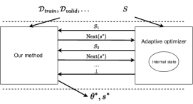
Figure 2: Compatibility of our method with adaptive optimizer is provided via the interaction between them, which are viewed as a unstateful interactive machine and a stateful interactive machine.

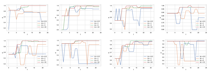
Figure 3: Plot of the fidelity score $\alpha$ over iterations. We run Algorithm 1 with different random seeds for 8 times. When $k\epsilon$ is small, the choice of hyperparameter will be easily to select an suboptimal candidate due to the overwelcoming amount of injected noise.

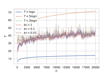
Figure 4: Plot of the empirical iterations $T=O(\log n)$ of Algorithm 1, compared with $T=c\cdot\log n,c=1,3,5$. The multiplier is sandwiched between 1 and 5, and approximately equal to 3.

4 Further Discussions

4.1 Compatibility with adaptive optimization

We briefly demonstrate the compatibility of our method with adaptive hyperparameter optimization techniques, such as Bayesian optimization. This is done by slightly modification of Algorithm 1 and simply viewing it as an unstateful interactive machine. Figure 4 describes the whole process. Consider a blackbox adaptive optimization method $\mathcal{O}$, which takes as input the hyperparameter space, then send some subset of hyperparameter candicates to our method, which runs one iteration and sends back the current value of $s^{*}$. Based on that feedback, $\mathcal{O}$ updates its internal state, and produce the next batch of hyperparameter candicates to our method. This process repeats until $O$ decides to terminates and stop sending candidates. Then our method outputs the final model parameter along with the hyperparameter.

However, it is worth to mention one subtle discrepancy in the feedback. Typically, the adaptive optimizer will obtain a feedback vector $u_{\mathcal{S}}\in(0,1)$ (the $i^{th}$ entry is the utility score of $S_{i}$. In this scenario, the feedback is sparse and binarized. Concretely, $i^{th}$ entry is equal to 1 if $i=s^{*}$ and 0 otherwise. Therefore, despite its compatibility, it remains still unclear whether adaptive optimization will bring a significant gain in efficiency while maintaining its proper functionality.

4.2 Experimental evaluation

In differential privacy, we usually care about the constant multiplier of the asympotical bound. The above theoretical analysis shows that the total iteration $T$ is bounded by $O(\log n)$. To help develop some sense of the actual constant multiplier of $\log n$, Figure 4 plots the the empirical relation between total iterations $T$ and $n:=\frac{u^{*}-u_{0}}{g}$, where the number of hyperparameters $|\mathcal{S}|$ is set to be 100 and the utility score is independently drawn from the uniform distribution over $(0,1)$. The experiment is repeated 10 times and the mean and standard deviation is reported. We can see that the multiplier is sandwiched between 1 and 5, and approximately equal to 3. It is worth noting that the larger $k\epsilon$ is, the larger of the variance will be, resulting from the increase amount of noise.

To evaluate the quality of the selected hyperparameter, Figure 3 plots the fidelity score $\alpha_{t}$ over iterations, in which we define the fidelity score $\alpha_{t}$ at iteration $t$ as

$$\alpha_{t}=\frac{u_{s^{*}}^{(t)}}{u^{*}}$$ (19)

where the concerned value is the final fidelity at the last iteration, i.e., $\alpha_{T}$. Overall, we can see that the larger $k\epsilon$ is, the higher and more stable the final fidelity score will be, which agrees with the trade-offs between privacy and accuracy. Specifically, we can see that when $k\epsilon=0.5$, it is unlikely to achieve a reasonable fidelity score. In contrast, when $k\epsilon=5$ or $10$, the fidelity score growth is much more stable and converges towards 1 rapidly. This experiment suggests that one heuristic choice of $k$ is to choose $k\geq 5/\epsilon$.

5 Conclusions

In this paper, we propose a machine learning algorithm-agnostic framework for hyperparameter tuning with differential privacy within constant privacy overhead. Compared to existing differentially private hyperparameter tuning methods that suffer from large hyperparameter search space, our additional privacy loss parameter is free from the size of the hyperparameter candidates set and the original privacy parameter of private training. Instead, it correlates with the final utility of the tuned model and is upper-bounded by the logarithm of the utility term. Therefore, it allows us to perform hyperparameter tuning on a larger range, even with a grid search, leading to potentially higher utility. We believe that our work would be meaningful in the field of privacy-preserving machine learning, and would be valuable for future research in this area.

Limitations. To realize the functionality of utility evaluation with low sensitivity, we partition the training dataset into $k$ parts. We note that this requires the number of training samples to be sufficiently large, e.g., $k\geq 5/\epsilon$. Otherwise, we are not able to obtain a reasonable fidelity. In addition, if $k$ is too small, i.e., $k=O(|\mathcal{D}_{train}|)$, each partition will have too little training data, leading to overfitting. We also note that it increases the computational cost of hyperparameter tuning by a factor of $k$. One positive aspect is that our method is compatible with adaptive optimization, which can help us save a huge amount of computation. Despite its compatibility, our method may not be immediately applicable to the existing adaptive approaches due to the restricted access of the utility scores, which we leave as potential future work.

References

- Abadi et al. (2016) Martín Abadi, Andy Chu, Ian J. Goodfellow, H. Brendan McMahan, Ilya Mironov, Kunal Talwar, and Li Zhang. Deep learning with differential privacy. In Proceedings of the 2016 ACM SIGSAC Conference on Computer and Communications Security, pages 308–318, 2016.
- Bassily et al. (2014) Raef Bassily, Adam Smith, and Abhradeep Thakurta. Private empirical risk minimization: Efficient algorithms and tight error bounds. In IEEE 55th Annual Symposium on Foundations of Computer Science, pages 464–473, 2014.
- Chaudhuri and Vinterbo (2013) Kamalika Chaudhuri and Staal A Vinterbo. A stability-based validation procedure for differentially private machine learning. Advances in Neural Information Processing Systems, 26, 2013.
- Dwork et al. (2006) Cynthia Dwork, Frank McSherry, Kobbi Nissim, and Adam Smith. Calibrating noise to sensitivity in private data analysis. In Theory of Cryptography Conference, pages 265–284, 2006.
- Dwork et al. (2009) Cynthia Dwork, Moni Naor, Omer Reingold, Guy N Rothblum, and Salil Vadhan. On the complexity of differentially private data release: Efficient algorithms and hardness results. In Proceedings of the 41st annual ACM Symposium on Theory of Computing, pages 381–390, 2009.
- Dwork et al. (2010) Cynthia Dwork, Guy N Rothblum, and Salil Vadhan. Boosting and differential privacy. In 2010 IEEE 51st Annual Symposium on Foundations of Computer Science, pages 51–60, 2010.
- Dwork et al. (2014) Cynthia Dwork, Aaron Roth, et al. The algorithmic foundations of differential privacy. Foundations and Trends in Theoretical Computer Science, 9(3–4):211–407, 2014.
- Kairouz et al. (2015) Peter Kairouz, Sewoong Oh, and Pramod Viswanath. The composition theorem for differential privacy. In International Conference on Machine Learning, pages 1376–1385, 2015.
- Kolluri et al. (2022) Aashish Kolluri, Teodora Baluta, Bryan Hooi, and Prateek Saxena. Lpgnet: Link private graph networks for node classification. In Proceedings of the 2022 ACM SIGSAC Conference on Computer and Communications Security, pages 1813–1827, 2022.
- Lee and Kifer (2021) Jaewoo Lee and Daniel Kifer. Scaling up differentially private deep learning with fast per-example gradient clipping. Proceedings on Privacy Enhancing Technologies, 2021(1), 2021.
- Liu and Talwar (2019) Jingcheng Liu and Kunal Talwar. Private selection from private candidates. Proceedings of the 51st ACM Symposium on Theory of Computing, page 298–309, 2019.
- Mockus et al. (1978) Jonas Mockus, Vytautas Tiesis, and Antanas Zilinskas. The application of bayesian methods for seeking the extremum. Towards global Optimization, 2(117-129):2, 1978.
- Mohapatra et al. (2022) Shubhankar Mohapatra, Sajin Sasy, Xi He, Gautam Kamath, and Om Thakkar. The role of adaptive optimizers for honest private hyperparameter selection. pages 7806–7813, 2022.
- Nissim et al. (2007) Kobbi Nissim, Sofya Raskhodnikova, and Adam Smith. Smooth sensitivity and sampling in private data analysis. In Proceedings of the 39th Annual ACM Symposium on Theory of Computing, pages 75–84, 2007.
- Papernot and Steinke (2022) Nicolas Papernot and Thomas Steinke. Hyperparameter tuning with renyi differential privacy. In International Conference on Learning Representations, 2022.
- Papernot et al. (2017) Nicolas Papernot, Martín Abadi, Úlfar Erlingsson, Ian J. Goodfellow, and Kunal Talwar. Semi-supervised knowledge transfer for deep learning from private training data. In Proceedings of 5th International Conference on Learning Representations, 2017.
- Papernot et al. (2018) Nicolas Papernot, Shuang Song, Ilya Mironov, Ananth Raghunathan, Kunal Talwar, and Úlfar Erlingsson. Scalable private learning with PATE. In Proceedings of 6th International Conference on Learning Representations, 2018.
- Sajadmanesh and Gatica-Perez (2021) Sina Sajadmanesh and Daniel Gatica-Perez. Locally private graph neural networks. In Proceedings of the 2021 ACM SIGSAC Conference on Computer and Communications Security, pages 2130–2145, 2021.
- Shokri et al. (2017) Reza Shokri, Marco Stronati, Congzheng Song, and Vitaly Shmatikov. Membership inference attacks against machine learning models. In IEEE Symposium on Security and Privacy, pages 3–18, 2017.
- Song et al. (2013) Shuang Song, Kamalika Chaudhuri, and Anand D Sarwate. Stochastic gradient descent with differentially private updates. In IEEE Global Conference on Signal and Information Processing, pages 245–248, 2013.
- Swersky et al. (2013) Kevin Swersky, Jasper Snoek, and Ryan P Adams. Multi-task bayesian optimization. Advances in Neural Information Processing Systems, 26, 2013.
- Tramer and Boneh (2020) Florian Tramer and Dan Boneh. Differentially private learning needs better features (or much more data). arXiv preprint arXiv:2011.11660, 2020.
- Tramèr and Boneh (2021) Florian Tramèr and Dan Boneh. Differentially private learning needs better features (or much more data). In 9th International Conference on Learning Representations, 2021.