Adaptive Stochastic Variance Reduction
for Non-convex Finite-Sum Minimization

Abstract.

We propose an adaptive variance-reduction method, called AdaSpider, for minimization of $L$-smooth, non-convex functions with a finite-sum structure. In essence, AdaSpider combines an AdaGrad-inspired [16, 40], but a fairly distinct, adaptive step-size schedule with the recursive stochastic path integrated estimator proposed in Fang et al. [19]. To our knowledge, AdaSpider is the first parameter-free non-convex variance-reduction method in the sense that it does not require the knowledge of problem-dependent parameters, such as smoothness constant $L$, target accuracy $\epsilon$ or any bound on gradient norms. In doing so, we are able to compute an $\epsilon$-stationary point with $\tilde{O}\left(n+\sqrt{n}/\epsilon^{2}\right)$ oracle-calls, which matches the respective lower bound up to logarithmic factors.

1. Introduction

This paper studies smooth, non-convex minimization problems with the following finite-sum structure:

$$\min_{x\in\mathbb{R}^{d}}f(x):=\frac{1}{n}\sum_{i=1}^{n}f_{i}(x),$$ (Prob)

where each component function $f_{i}:\mathbb{R}^{d}\to\mathbb{R}$ is $L$-smooth and is possibly non-convex, and we further assume $f$ is also non-convex. We seek to find an $\epsilon$-approximate first-order stationary point $\hat{x}$ of $f$, such that $\lVert\nabla f(\hat{x})\rVert\leq\epsilon$, where $\epsilon>0$ is the accuracy of the desired solution.

This structure captures many interesting learning problems from empirical risk minimization to training of neural networks. First-order methods have been the standard choice for solving (Prob), due to their efficiency and favorable practical behavior. In that regard, while gradient descent (Gd) requires $O(n/\epsilon^{2})$ gradient computations, stochastic gradient descent (Sgd) requires $O(1/\epsilon^{4})$ overall gradient computations. In many interesting machine learning applications $n$ tends to be large, e.g., training a neural network for image classification with very big image datasets [14], hence Sgd typically leads to better practical performance.

To leverage the best of both regimes, Gd and Sgd, the so-called variance reduction (VR) framework combines the faster convergence rate of Gd with the low per-iteration complexity of Sgd. Originally proposed for solving strongly-convex problems [24, 13, 42], variance reduction frameworks essentially generate low-variance gradient estimates by maintaining a balance between periodic full gradient computations and stochastic (mini-batch) gradients. VR methods and their theoretical behavior for convex problems have been well-studied under various problem setups and assumptions, including $\mu$-strongly convex functions with $O(n+(L/\mu)\log(1/\epsilon))$ complexity [24, 42, 13]; $\mu$-strongly convex functions with accelerated $O(n+\sqrt{L/\mu}\log(1/\epsilon))$ complexity [2, 29, 47] and smooth, convex functions with $\tilde{O}(n+1/\epsilon)$ complexity [58, 47, 15]. For non-convex minimization, earlier attempts extended the existing VR frameworks, achieving the first rates of order $O(n+n^{2/3}/\epsilon^{2})$ with sub-optimal dependence on $n$ [45, 55, 1, 35]. The most recent non-convex VR methods [18, 51, 36, 44, 37] close this gap and achieve the optimal gradient oracle complexity of $O(n+\sqrt{n}/\epsilon^{2})$ [18].

Adaptivity and First-order Optimization

The selection of the step-size is of great importance in both the theoretical and practical performance of first-order methods, including the aforementioned VR methods. In the case of $L$-smooth minimization, first-order methods need the knowledge of $L$ so as to adequately select their step-size [41], otherwise the method is not guaranteed to be convergent and might even diverge [15, 38]. To elucidate, classical analysis relies on the (expected) descent property and guarantees that the algorithm monotonically makes progress every iteration. To enforce this property everywhere on the optimization landscape, one needs to pick the step-size as $\gamma_{t}\leq O(1/L)$, which restricts the step length of the algorithm with respect to the worst-case constant $L$. On the other hand, estimating the smoothness constant for an objective of interest, such as neural networks, is a very hard task [21]. At the same time, using crude bounds on the smoothness constant leads to very small step-sizes and consequently to poorer convergence. In practice the step-size is tuned through an empirical search over a range of hand-picked values that adds a considerable computational overhead and burden. In order to alleviate the burden of tuning process, we need step-sizes that adjust in accordance with the optimization path.

A popular line of research studies first-order methods that adaptively select their step-size by taking advantage of the previously produced point. In many settings of interest, these adaptive methods are able to guarantee optimal convergence rates without requiring the knowledge of the smoothness constant $L$ while they often admit superior empirical performance due to their ability to decrease the step-size according to the local geometry of the objective function. Inspired by AdaGrad introduced in the concurrent seminal works of [16] [39], a recent line of works [31, 26, 25, 17] propose adaptive gradient methods that given access to noiseless gradient-estimates achieve accelerated rates in the case of $L$-smooth convex minimization without requiring the knowledge of smoothness constant $L$. Similarly, Ene et al. [17] and Antonakopoulos et al. [5] propose adaptive methods with optimal convergence rates for monotone variational inequalities while Antonakopoulos et al. [6] provide adaptive methods for monotone variational inequalities assuming access to relative noise gradient-estimates. Hsieh et al. [23] and Vu et al. [50] study the convergence properties of adaptive first-order methods for routing and generic games.

Adaptive non-convex methods for General Noise Related to our work is a recent line of papers studying adaptive first-order methods under the general noise model. In this setting, a method is assumed to access unbiased stochastic estimate of the gradient with bounded variance. This is a more general setting than finite-sum optimization that comes with worse lower bounds, i.e. $\Omega(1/\epsilon^{4})$ gradient-estimates are needed so as to compute an $\epsilon$-stationary point. A recent line of works study adaptive first-order methods that are able to achieve near-optimal oracle-complexity while being oblivious to the smoothness constant $L$ and the variance of the estimator [52, 20, 34, 27]. For example Ward et al. [52] established that the adaptive method called AdaGrad-Norm is able to achieve $\tilde{O}(1/\epsilon^{4})$ gradient-complexity in the general noise model. In their recent work, Faw et al. [20] significantly extended the results of Ward et al. [52] by showing that AdaGrad-Norm achieves the same rates even in case the gradient admits unbounded norm (a restrictive assumption in [52]) while their result persists even if the variance increases with the gradient norm. In the slightly more restrictive setting at which the objective function $f(x):=\mathbb{E}_{\xi\sim\mathcal{D}}g(x,\xi)$ where each estimate $g(x,\xi)$ is $L$-smooth with respect to $x$ for all $\xi$, Levy et al. [32] proposed an adaptive method called STORM++ that achieves $O(1/\epsilon^{3})$ gradient-complexity and that removes the requirement of the knowledge on problem parameters (e.g., smoothness constant, absolute bounds on gradient norms) that the original STORM method proposed by Cutkosky et al. [12] requires. The latter gradient-complexity matches the $\Omega(1/\epsilon^{3})$ lower bound of Arjevani et al. [7].

Adaptivity and Finite-Sum minimization

In parallel with what we discussed earlier, existing variance-reduction methods (VR) crucially need to know the smoothness constant $L$ to select their step-size appropriately to guarantee their convergence. To this end, the following natural question arises

Can we design adaptive VR methods that achieve the optimal gradient computation complexity?

Li et al. [33] and Tan et al. [49] were the first to propose adaptive variance-reduction methods by using the Barzilai-Borwein step-size [8]. Despite their promising empirical performance, these methods do not admit formal convergence guarantees. When the objective function $f$ in (Prob) is convex, [15] recently proposed an adaptive VR method requiring $O(n+1/\epsilon)$ gradient computation while, shortly after, [38] proposed an accelerated adaptive VR method requiring $O(n+\sqrt{n}/\sqrt{\epsilon})$ gradient computations.

To the best of our knowledge, there is no adaptive VR method in the case where $f$ is non-convex. We remark that $f$ being non-convex captures the most interesting settings such as minimizing the empirical loss of deep neural network where each $f_{i}$ stands for the loss with respect to $i$-th data point and thus is a non-convex function in the parameters of the neural architecture. Through this particular example, we could motivate adaptive VR methods in two fronts: first, even estimating the smoothness constant $L$ of a deep neural network is prohibitive [21], and at the same time, the parameter $n$ in (Prob) equals the number of data samples, which can be very large in practice and is prohibitive for the use of deterministic methods.

Contribution and Techniques

In this work we present an adaptive VR method, called AdaSpider, that converges to an $\epsilon$-stationary point for (Prob) by using $\tilde{O}(n+\sqrt{n}L^{2}/\epsilon^{2})$ gradient computations. Our gradient complexity bound matches the existing lower bounds up to logarithmic factors [19].

$f(x)$	Non-Adaptive VR	Adaptive VR	Complexity Lower Bound
convex	$\tilde{O}\left(n+\sqrt{\frac{n}{\epsilon}}\right)$	$\tilde{O}\left(n+\sqrt{\frac{n}{\epsilon}}\right)$	$\Omega(n+\sqrt{\frac{n}{\epsilon}})$
($\epsilon$-opt. solution)	[28]	[38]	[53]
convex	$\tilde{O}\left(n+\frac{1}{\epsilon}\right)$	$\tilde{O}\left(n+\frac{1}{\epsilon}\right)$	$\Omega(n+\sqrt{\frac{n}{\epsilon}})$
($\epsilon$-opt. solution)	[57]	[15]	[53]
non-convex	$O\left(n+\frac{\sqrt{n}}{\epsilon^{2}}\right)$	$\tilde{O}\left(n+\frac{\sqrt{n}}{\epsilon^{2}}\right)$	$\Omega\left(n+\frac{\sqrt{n}}{\epsilon^{2}}\right)$
($\epsilon$-stat. point)	[19]	This work	[19]

Table 1. In the following table we present the gradient computation complexity of the existing non-adaptive and adaptive variance reduction methods for both convex and non-convex finite-sum minimization. Since for there are multiple non-adaptive VR methods, we present the earliest-proposed method matching up to logarithmic factors the respective lower bounds.

AdaSpider combines an adaptive step-size schedule in the lines proposed by AdaGrad [16] with the variance-reduction mechanism based on the stochastic path integrated differential estimator of the Spider algorithm [19]. More precisely, AdaSpider selects the step-size by aggregating the norm of its recursive estimator, while following a single-loop structure as in Fang et al. [19].

Our contributions and techniques can be summarized as follows:

• To our knowledge, AdaSpider is the first parameter-free method in the sense that it is both accuracy-independent and is oblivious to the knowledge of any problem parameters including $L$. Moreover, $\epsilon$-independence enables us to provide any-iterate guarantees. While Spider needs both $\epsilon$ and $L$ to set its step-size as $\min(\frac{\epsilon}{L\sqrt{n}\lVert\nabla_{t}\rVert,},\frac{1}{2\sqrt{n}L})$ to achieve optimal gradient complexity [19], all other existing non-convex methods must know at least the value of $L$ in order to guarantee convergence [4, 51].

• We introduce a novel step-size schedule $\gamma_{t}:=n^{-1/4}\left(\sqrt{n}+\sum_{s=0}^{t}\lVert\nabla_{s}\rVert^{2}\right)^{-1/2}$ where $\nabla_{s}$ is the recursive variance-reduced estimator at round $s$. By identifying a unique additive/multiplicative form for integrating $n$, we manage to achieve optimal dependence on the number of components. We note that Adaspider can be viewed as Spider with the step-size of AdaGrad-Norm [20, 52, 48, 43] were the parameters are respectively selected as $\eta:=n^{1/4}$ and $b_{0}^{2}:=\sqrt{n}$ [20].

• We show how to combine the above adaptive step-size schedule with the recursive Spider estimator in order to ensure that the average variance $\frac{1}{T}\sum_{t=0}^{T-1}\mathbb{E}\left[\lVert\nabla_{t}-\nabla f(x_{t})\rVert\right]$ decays at a rate $\tilde{O}\left(n^{1/4}/\sqrt{T}\right)$. This might be of independent interest for other variance reduction techniques.

We follow a novel technical path that uses the adaptivity of the step-size to bound the overall variance of the process. This fact differentiates our approach from the previous adaptive and non adaptive VR approaches (see Section 4 for further details) and provides us a surprisingly concise analysis.

Remark 1.

Our convergence results do not require bounded gradients that is typically a restrictive assumption that the analysis of the adaptive methods for stochastic optimization require. We overcome this obstacle by using the fact $\lVert x_{t}-x_{t-1}\rVert\leq 1$ (due to the step-size selection) and thus $\lVert\nabla f(x_{t})-\nabla f(x_{t-1})\rVert\leq L\lVert x_{t}-x_{t-1}\rVert\leq L$. The latter leads to the following upper bound on the gradient norm, $\lVert\nabla f(x_{t})\rVert\leq LT+\lVert\nabla f(x_{0})\rVert$ that however leads to only a logarithmic overhead in the final bound (see Lemma 2). A similar idea is used by Faw et al. [20] (Lemma $2$) in order to remove the bounded gradient assumption on the convergence rates of AdaGrad-Norm under general noise.

2. Setup and Preliminaries

During the whole of this manuscript, we consider that the non-convex objective function $f:\mathbb{R}^{d}\mapsto\mathbb{R}$ possesses a finite-sum structure

$$f(x)=\frac{1}{n}\sum_{i=1}^{n}f_{i}(x)$$

where each component function $f_{i}$ is $L$-smooth (or alternatively has $L$-Lipschitz gradient) and (possibly) non-convex. To quantify the performance of our algorithm within the context of non-convex minimization, we want to find an $\epsilon$-first order stationary point $\hat{x}\in\mathbb{R}^{d}$ such that

$$\lVert\nabla f(\hat{x})\rVert\leq\epsilon.$$

For notational simplicity we define $\lVert\cdot\rVert$ as the Euclidean norm. Then, we say that a continuously differentiable function $f$ is $L$-smooth if

$$\lVert\nabla f(x)-\nabla f(y)\rVert\leq L\lVert x-y\rVert,$$ (2.1)

which admits the following equivalent form,

$$f(x)\leq f(y)+\nabla f(y)^{\top}(x-y)+\frac{L}{2}\lVert x-y\rVert^{2}~{}~{}~{}\text{for all }x,y\in\mathbb{R}^{d}.$$ (2.2)

Observe that smoothness of each component immediately suggests that objective $f$ is $L$-smooth itself. Since we are studying randomized algorithms for finite-sum minimization problems, we do not consider any variance bounds on the gradients of components. We only assume that we have access to an oracle which returns the gradient of individual components when queried.

3. Adaptive SPIDER algorithm and convergence results

In this section, we present our adaptive variance reduction method, called AdaSpider (Algorithm 1) which exploits the variance reduction properties of the stochastic path integrated differential estimator proposed in [19] while combining it with an AdaGrad-type step-size construction [16]. Unlike the original Spider method [19], our algorithm admits anytime guarantees, i.e., we don’t need to specify the accuracy $\epsilon$ a priori. Additionally, our algorithm does not need to know the smoothness parameter $L$ and guarantees convergence without any tuning procedure.

Algorithm 1 Adaptive SPIDER (AdaSpider)

Input: $x_{0}\in\mathbb{R}^{d},\beta_{0}>0,G_{0}>0$

1:  $G\leftarrow 0$

2:  for $t=0,...,T-1$ do

3:     if  $t~{}\mathrm{mod}~{}n=0$ then

4:        $\nabla_{t}\leftarrow\nabla f(x_{t})$

5:     else

6:        pick $i_{t}\in\{1,\ldots,n\}$ uniformly at random

7:        $\nabla_{t}\leftarrow\nabla f_{i_{t}}(x_{t})-\nabla f_{i_{t}}(x_{t-1})+\nabla_{t-1}$

8:     end if

9:     $\gamma_{t}\leftarrow 1/\left(n^{1/4}\beta_{0}\sqrt{n^{1/2}G_{0}^{2}+\sum_{s=0}^{t}\lVert\nabla_{s}\rVert^{2}}\right)$

10:     $x_{t+1}\leftarrow x_{t}-\gamma_{t}\cdot\nabla_{t}$

11:  end for

12:  return uniformly at random $\{x_{0},\ldots,x_{T-1}\}$.

Remark 2.

In Algorithm 1 the units of $G_{0}$ are the same with the units of $\nabla f(x_{t})$ i.e. $f/x$ while the units of $\beta_{0}$ are $x^{-1}$. The latter is important so that the step-size $\gamma_{t}$ takes the right units i.e. $x^{2}/f$.

As Algorithm 1 indicates, AdaSpider performs a full-gradient computation every $n$ iterations while in the rest iterations updates the variance-reduced gradient estimator in a recursive manner, $\nabla_{t}\leftarrow\nabla f_{i_{t}}(x_{t})-\nabla f_{i_{t}}(x_{t-1})+\nabla_{t-1}$. The adaptive nature of AdaSpider comes from the selection of the step-size at Step $9$ that only depends on the norms of estimates produced by the algorithm in the previous steps.

Before presenting the formal convergence guarantees of AdaSpider (stated in Theorem 1), we present the cornerstone idea behind its design and motivate the analysis for controlling the overall variance of the process through the adaptivity of the step-size. This conceptual novelty differentiates our work form the previous adaptive VR methods [15, 38] at which the adaptivity of the step-size is only used for adapting to the smoothness constant $L$, and their constructions come with additional challenges in bounding the variance. As a result, the following challenge is the first to be tackled by the design of a VR method.

Challenge 1.

Does the average variance of the estimator, $\frac{1}{T}\sum_{t=0}^{T-1}\mathbb{E}\left[\lVert\nabla_{t}-\nabla f(x_{t})\rVert\right]$, diminishes at a sufficiently fast rate?

Up next we explain why combining the variance-reduction estimator of Step $7$ with the adaptive step-size of Step $9$ provides a surprisingly concise answer to Challenge 1. We remark that Spider is able to control the variance at any iterations by choosing $\gamma_{t}:=\min(\frac{\epsilon}{L\sqrt{n}\lVert\nabla_{t}\rVert,},\frac{1}{2\sqrt{n}L})$ as step-size. The latter enforces the method to make tiny steps, $\lVert x_{t}-x_{t-1}\rVert\leq\epsilon/L\sqrt{n}$ which results in $\epsilon$-bounded variance at any iteration. The latter proposed SpiderBoost [51] provides the same gradient-complexity bounds with Spider but through the accuracy-independent step-size $\gamma=1/L$. SpiderBoost handles Challenge 1 by using a dense gradient-computations schedule combined with amortization arguments based on the descent inequality (this is why the knowledge of $L$ is necessary in its analysis). We remark that AdaSpider, despite being oblivious to $L$ and accuracy $\epsilon$, admits a significantly simpler analysis by exploiting the adaptability of its step-size.

In the rest of the section we present our approach to Challenge 1 and we conclude the section with Theorem 1 stating the formal convergence guarantees of AdaSpider.

Handling the variance with adaptive step-size We start with the following variance aggregation lemma that is folklore in (VR) literature (e.g. [56]).

Lemma 1.

Define the gradient estimator at point $x$ as $\nabla_{x}:=\nabla f_{i}(x)-\nabla f_{i}(y)+\nabla_{y}$ where $i$ is sampled uniformly at random from $\{1,\ldots,n\}$. Then,

$$\mathbb{E}\left[\lVert\nabla_{x}-\nabla f(x)\rVert^{2}\right]\leq L^{2}\lVert x-y\rVert^{2}+\mathbb{E}\left[\lVert\nabla_{y}-\nabla f(y)\rVert^{2}\right]$$

Now, let us apply Lemma 1 on Spider estimator, $\nabla_{t}:=\nabla f_{i_{t}}(x_{t})-\nabla f_{i_{t-1}}(x_{t})+\nabla_{t-1}$ to measure its variance at step $x_{t}$.

$$\mathbb{E}\left[\lVert\nabla_{t}-\nabla f(x_{t})\rVert^{2}\right] \leq L^{2}\mathbb{E}\left[\lVert x_{t}-x_{t-1}\rVert^{2}\right]+\mathbb{E}\left[\lVert\nabla_{t-1}-\nabla f(x_{t-1})\rVert^{2}\right]$$

$$\leq L^{2}\mathbb{E}\left[\gamma^{2}_{t-1}\lVert\nabla_{t-1}\rVert^{2}\right]+\mathbb{E}\left[\lVert\nabla_{t-1}-\nabla f(x_{t-1})\rVert^{2}\right]$$

$$\leq L^{2}\mathbb{E}\left[\gamma^{2}_{t-1}\lVert\nabla_{t-1}\rVert^{2}\right]+\ldots+\mathbb{E}\left[\lVert\nabla_{t-(t~{}\mathrm{mod}~{}n)}-\nabla f(x_{t-(t~{}\mathrm{mod}~{}n})\rVert^{2}\right]$$

$$=\sum_{\tau=t-(t~{}\text{mod }n)+1}^{t-1}L^{2}\mathbb{E}\left[\gamma^{2}_{\tau}\cdot\lVert\nabla_{\tau}\rVert^{2}\right]$$

where the last equality follows by the fact $\mathbb{E}\left[\lVert\nabla_{t-(t~{}\mathrm{mod}~{}n)}-\nabla f(x_{t-(t~{}\mathrm{mod}~{}n})\rVert^{2}\right]=0$ since Algorithm 1 performs a full-gradient computations for every $t$ with $t~{}\mathrm{mod}~{}n=0$ (Step $3$ of Algorithm 1). By telescoping the summation we get,

$$\sum_{t=0}^{T-1}\mathbb{E}\left[\lVert\nabla_{t}-\nabla f(x_{t})\rVert^{2}\right]\leq\sum_{t=0}^{T-1}\sum_{\tau=t-(t~{}\text{mod }n)+1}^{t-1}L^{2}\mathbb{E}\left[\gamma^{2}_{\tau}\cdot\lVert\nabla_{\tau}\rVert^{2}\right]\leq L^{2}n\cdot\sum_{t=0}^{T-1}\mathbb{E}\left[\gamma_{t}^{2}\cdot\lVert\nabla_{t}\rVert^{2}\right]$$

where the $n$ factor on the right-hand side is due to the fact that each term $\mathbb{E}\left[\gamma_{t}^{2}\lVert\nabla_{t}\rVert^{2}\right]$ appears at most $n$ times in the total summation. To this end, using the structure of the stochastic path integrated differential estimator we have been able to bound the overall variance of the process as follows,

$$\sum_{t=0}^{T-1}\mathbb{E}\left[\lVert\nabla_{t}-\nabla f(x_{t})\rVert^{2}\right]\leq L^{2}n\cdot\sum_{t=0}^{T-1}\mathbb{E}\left[\gamma_{t}^{2}\cdot\lVert\nabla_{t}\rVert^{2}\right]$$

However it is not clear at all why the above bound is helpful. At this point the adaptive selection of the step-size (Step $9$ in Algorithm 1) comes into play by providing the following surprisingly simple answer,

$$\sum_{t=0}^{T-1}\mathbb{E}\left[\lVert\nabla_{t}-\nabla f(x_{t})\rVert^{2}\right]\leq L^{2}n~{}\mathbb{E}\left[\sum_{t=0}^{T-1}\gamma_{t}^{2}\cdot\lVert\nabla_{t}\rVert^{2}\right]$$

$$= \frac{L^{2}\sqrt{n}}{\beta_{0}^{2}}~{}\mathbb{E}\left[\sum_{t=0}^{T-1}\frac{\lVert\nabla_{t}\rVert^{2}/G_{0}^{2}}{\sqrt{n}+\sum_{s=0}^{t}\lVert\nabla_{s}\rVert^{2}/G_{0}^{2}}\right]\leq\frac{L^{2}\sqrt{n}}{\beta_{0}^{2}}\log\left(1+\mathbb{E}\left[{\sum_{t=0}^{T-1}\lVert\nabla_{t}\rVert^{2}/G_{0}^{2}}\right]\right)$$

where the last inequality comes from Lemma 7. To finalize the bound, we require the following expression that follows by the fact that $\gamma_{t}\leq 1/\lVert\nabla_{t}\rVert$ and thus $\lVert x_{t}-x_{t-1}\rVert\leq 1$.

Lemma 2.

Let $x_{0},x_{1},\ldots,x_{T}$ the points produced by Algorithm 1. Then,

$$\sum_{t=0}^{T-1}\lVert\nabla_{t}\rVert^{2}\leq\mathcal{O}\left(n^{2}T^{3}\cdot\left(\frac{L^{2}}{\beta_{0}^{2}}+\lVert\nabla f(x_{0})\rVert^{2}\right)\right)$$

In simple terms, Lemma 2 helps us avoid the bounded gradient norm assumption that is common among adaptive non-convex methods. As a result, AdaSpider admits the following cumulative variance bound,

$$\sum_{t=0}^{T-1}\mathbb{E}\left[\lVert\nabla_{t}-\nabla f(x_{t})\rVert^{2}\right]\leq O\left(\frac{L^{2}\sqrt{n}}{\beta_{0}^{2}}\log\left(1+nT\cdot\left(\frac{L}{\beta_{0}G_{0}}+\frac{\lVert\nabla f(x_{0})\rVert}{G_{0}}\right)\right)\right).$$ (3.1)

Remark 3.

To this end one might notice that using a more aggressive $n$ dependence on $\gamma_{t}$ leads to smaller variance of the estimator which is obviously favorable. However more aggressive dependence on $n$ leads to smaller step-sizes and thus to sub-optimal overall gradient-computation complexity. In Section 4, we explain why the optimal way to inject the $n$ dependence into the step-size is through the simultaneous multiplicative/additive way described in Step $9$ of AdaSpider that may seem unintuitive on the first sight.

We will conclude this discussion with a complementary remark on the interplay between our adaptive step-size and the convergence rate. As we demonstrated in Eq. (3.1), using a data-adaptive step-size leads to a decreasing variance bound in an amortized sense as opposed to any iterate variance bound of Spider. The trade-off in our favor is the parameter-free step-size that is independent of $\epsilon$ and $L$. For a fair exposition of our results, notice that the aforementioned advantages of an adaptive step-size comes at an additional $\log(T)$ term in our final bound due to Eq. (3.1). This has a negligible effect on the convergence as even in the large iteration regime when $T$ is in the order billions, it amounts to a small constant factor.

We conclude the section with Theorem 1 that formally establishes the convergence rate of AdaSpider. The proof of Theorem 1 is deferred for the next section.

Theorem 1.

Let $x_{0},x_{1},\ldots,x_{T-1}$ be the sequence of points produced by Algorithm 1 in case $f(\cdot)$ is $L$-smooth. Let us also define $\Delta_{0}:=f(x_{0})-f^{\ast}$. Then,

$$\frac{1}{T}\sum_{t=0}^{T-1}\mathbb{E}\left[\lVert\nabla f(x_{t})\rVert\right]\leq O\left(n^{1/4}\cdot\frac{\Theta}{\sqrt{T}}\cdot\log\left(1+nT\cdot\left(\frac{L}{\beta_{0}G_{0}}+\frac{\lVert\nabla f(x_{0})\rVert}{G_{0}}\right)\right)\right)$$

where $\Theta=\Delta_{0}\cdot\beta_{0}+G_{0}+L/\beta_{0}+L^{2}/(\beta_{0}^{2}G_{0})$. Overall, Algorithm 1 with $\beta_{0}:=1$ and $G_{0}:=1$ needs at most $\tilde{O}\left(n+\sqrt{n}\cdot\frac{\Delta_{0}^{2}+L^{4}}{\epsilon^{2}}\right)$ oracle calls to reach an $\epsilon$-stationary point.

4. Sketch of Proof of Theorem 1

In this section we present the key steps for proving Theorem 1. We first use the triangle inequality to derive,

$$\sum_{t=0}^{T-1}\mathbb{E}\left[\lVert\nabla f(x_{t})\rVert\right]\leq\sum_{t=0}^{T-1}\mathbb{E}\left[\lVert\nabla_{t}-\nabla f(x_{t})\rVert\right]+\sum_{t=0}^{T-1}\mathbb{E}\left[\lVert\nabla_{t}\rVert\right]$$

We have previously discussed how to bound the first term in Section 3. More precisely, by the Jensen’s inequality and the arguments presented in Section 3, we obtain the following variance bound.

Lemma 3.

Let $x_{0},x_{1}\ldots,x_{T}$ the sequence of points produced by Algorithm 1. Then,

$$\sum_{t=0}^{T-1}\mathbb{E}\left[\lVert\nabla_{t}-\nabla f(x_{t})\rVert^{2}\right]\leq O\left(\frac{Ln^{1/4}}{\beta_{0}}\sqrt{\log\left(1+nT\cdot\left(\frac{L}{\beta_{0}G_{0}}+\frac{\lVert\nabla f(x_{0})\rVert}{G_{0}}\right)\right)}\right).$$

We continue with presenting how to treat the term $\sum_{t=0}^{T-1}\mathbb{E}\left[\lVert\nabla_{t}\rVert\right]$. By the smoothness of the function and through a telescopic summation one can easily establish the following bound,

$$\mathbb{E}\left[\sum_{t=0}^{T-1}\gamma_{t}\cdot\lVert\nabla_{t}\rVert^{2}\right]\leq 2(f(x_{0})-f^{\ast})+L\cdot\mathbb{E}\left[\sum_{t=0}^{T-1}\gamma_{t}^{2}\cdot\lVert\nabla_{t}\rVert^{2}\right]+\mathbb{E}\left[\sum_{t=0}^{T-1}\gamma_{t}\cdot\lVert\nabla f(x_{t})-\nabla_{t}\rVert^{2}\right]$$

As we explained in Section 3, the term $\mathbb{E}\left[\sum_{t=0}^{T-1}\gamma_{t}^{2}\cdot\lVert\nabla_{t}\rVert^{2}\right]$ can be upper bounded by the adaptability of the step-size $\gamma_{t}$. At the same time, using the adaptability of $\gamma_{t}$ we are able to establish that $\sum_{t=0}^{T-1}\mathbb{E}\left[\lVert\nabla_{t}\rVert\right]$ is at most $n^{1/4}\sqrt{T}\cdot\mathbb{E}\left[\sum_{t=0}^{T-1}\gamma_{t}\cdot\lVert\nabla_{t}\rVert^{2}\right]$. All the above are formally stated and established in Lemma 4 the proof of which is deferred to the appendix.

Lemma 4.

Let $x_{0},x_{1},\ldots,x_{T-1}$ the sequence of points produced by Algorithm 1 and $\Delta_{0}:=f(x_{0})-f^{\ast}$. Then,

$$\mathbb{E}\left[\sum_{t=0}^{T-1}\lVert\nabla_{t}\rVert\right]\leq\tilde{\mathcal{O}}\left(\Delta_{0}\cdot\beta_{0}+G_{0}+\frac{L}{\beta_{0}}+\mathbb{E}\left[\sum_{t=0}^{T-1}\gamma_{t}\lVert\nabla f(x_{t})-\nabla_{t}\rVert^{2}\right]\right)n^{1/4}\sqrt{T}.$$

Due to the use of the adaptive step-size $\gamma_{t}$, the estimator’s error and the step-size itself are dependent random variables, meaning that the weighted variance term $\mathbb{E}\left[\sum_{t=0}^{T-1}\gamma_{t}\lVert\nabla f(x_{t})-\nabla_{t}\rVert^{2}\right]$ cannot be handled by Lemma 1. To overcome the latter, we use the monotonic behavior of the step-size $\gamma_{t}$ to establish the following refinement of Lemma 1.

Lemma 5.

Let $x_{0},x_{1},\ldots$ the sequence of points produced by Algorithm 1. Then,

$$\mathbb{E}\left[\sum_{t=0}^{T-1}\gamma_{t}\cdot\lVert\nabla_{t}-\nabla f(x_{t})\rVert^{2}\right]\leq L^{2}n\cdot\mathbb{E}\left[\sum_{t=0}^{T-1}\gamma_{t}^{3}\cdot\lVert\nabla_{t}\rVert^{2}\right]$$

To this end we are ready to summarize the importance of simultaneous additive/multiplicative dependence of $\gamma_{t}$ in Step $9$ of Algorithm 1. This selection permits us to do achieve two orthogonal goals at the same time,

• Bounding the variance of the process, $\mathbb{E}\left[\sum_{t=0}^{T-1}\lVert\nabla_{t}-\nabla f(x_{t})\rVert\right]\leq\tilde{O}\left(n^{1/4}\sqrt{T}\right)$ (see Section 3 and Lemma 3).

• Bounding the sum, $\mathbb{E}\left[\sum_{t=0}^{T-1}\lVert\nabla_{t}\rVert\right]\leq\tilde{O}\left(n^{5/4}\sqrt{T}\cdot\mathbb{E}\left[\sum_{t=0}^{T-1}\gamma_{t}^{3}\lVert\nabla_{t}\rVert^{2}\right]\right)$ (see Lemma 4 and Lemma 5).

The third important thing that the selection of $\gamma_{t}$ does is that it permits us to upper bound the term $\tilde{O}\left(n^{5/4}\ \mathbb{E}\left[\sum_{t=0}^{T-1}\gamma_{t}^{3}\lVert\nabla_{t}\rVert^{2}\right]\right)$ by $\tilde{O}\left(n^{1/4}\right)$. The proof of the latter upper bound can be found in the proof of Theorem 1 that due to lack of space is deferred to appendix. It is interesting that all the above three different purposes can be handled by selecting $\gamma_{t}=n^{-1/4}\beta_{0}(\sqrt{n}\cdot G_{0}^{2}+\sum_{s=0}^{t}\lVert\nabla_{s}\rVert^{2})^{-1/2}$.

5. Experiments

We complement our theoretical findings with an evaluation of the numerical performance of the algorithm under different experimental setups. We aim to highlight the sample complexity improvements over simple stochastic methods, while displaying the advantages of adaptive step-size strategies. For that purpose we design two setups; first, we consider the minimization of a convex loss with a non-convex regularizer in the sense of Wang et al. [51] and in a second part we consider an image classification task with neural networks.

5.1. Convex loss with a non-convex regularizer

We consider the following problem:

$$\min_{x\in\mathbb{R}^{d}}\frac{1}{n}\sum_{i=1}^{n}\ell(x,(a_{i},b_{i}))+\lambda g(x)$$

where $\ell(x,(a_{i},b_{i}))$ is the loss with respect to the decision variable/weights $x$ with $(a_{i},b_{i})$ denoting the (feature vector, label) pair. We select $g=\sum_{i=1}^{d}\frac{x_{i}^{2}}{1+x_{i}^{2}}$, similar to Wang et al. [51], where the subscript denotes the corresponding dimension of $x$. We compare AdaSpider against the original Spider, SpiderBoost, Svrg, AdaSvrg and two non-VR methods, Sgd and AdaGrad. We picked two datasets from LibSVM, namely a1a, mushrooms. We initialize each algorithm from the same point and repeat the experiments 5 times, then report the mean convergence with standard deviation as the shaded region around the mean curves. We tune the algorithms by executing a parameter sweep for their initial step-size over an interval of values which are exponentially scaled as $\left\{{10^{-3},10^{-2},...,10^{2},10^{3}}\right\}$. After tuning the algorithms on one dataset, we run them with the same parameters for the others.

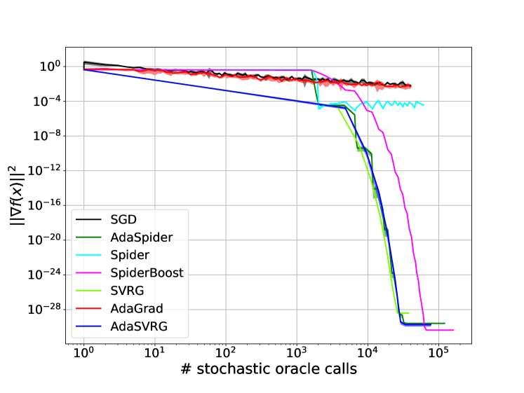
(a) a1a

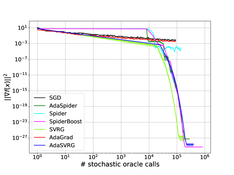
(b) mushrooms

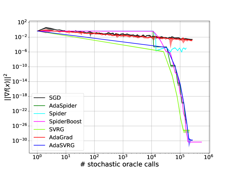
(c) a6a

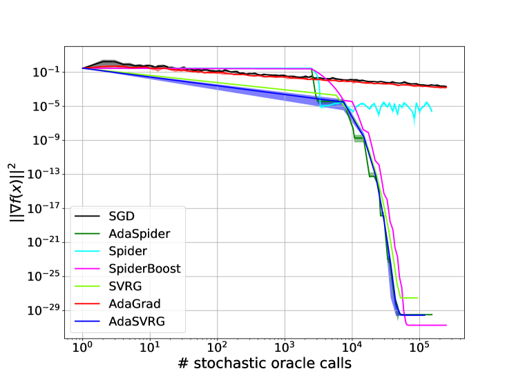
(d) w1a

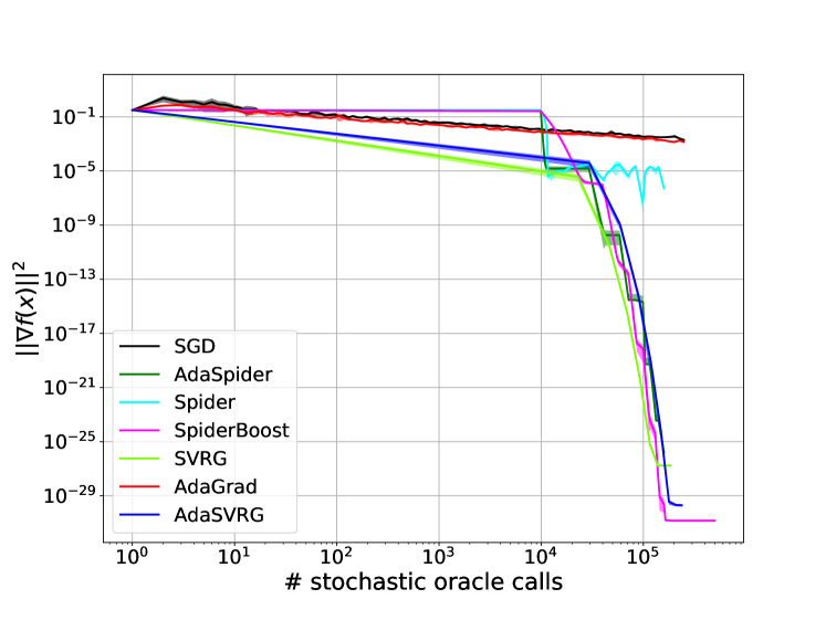
(e) w5a

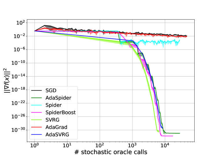
(f) ionosphere-scale

Figure 1. Logistic regression with non-convex regularizer on LibSVM datasets

First, we clearly observe the difference between Sgd & AdaGrad, and the rest of the pack, which demonstrates the superior sample complexity of VR methods in general. Among VR algorithms, there does not seem to be any concrete differences with similar convergence, except for Spider. The performance of AdaSpider is on par with other VR methods, and superior to Spider. The unexpected behavior of Spider algorithm has previously been documented in Wang et al. [51]. From a technical point of view, this behavior is predominantly due to the accuracy dependence in the step-size, making the step-size unusually small. We had to run Spider beyond its prescribed setting and tune the step-size with a large initial value to make sure the algorithm makes observable progress.

5.2. Experiments with neural networks

In our second setup, we train neural networks with our variance reduction scheme. Our focus is on standard image classification tasks trained with the cross entropy loss [9, 10]. Denoting by $C$ the number of classes, the considered datasets in this section consist of $n$ pairs $(a_{i},b_{i})$ where $a_{i}$ is a vectorized image and $b_{i}\in\mathbb{R}^{C}$ is a one-hot encoded class label. A neural network is parameterized with weights $x\in\mathbb{R}^{d}$ and its output on is denoted $\text{net(x, a)}\in\mathbb{R}^{C}$, where $a$ is the input image. The training of the network consists of solving the following optimization problem: $\min_{x\in\mathbb{R}^{d}}\frac{1}{n}\sum_{i=1}^{n}\left(-b_{i}^{\top}\text{net}(x,a_{i})+\texttt{logsumexp}(\text{net}(x,a_{i}))\right).$ This is the default setup for doing image classification and we test our algorithm on two benchmark datasets : MNIST[30] and FashionMNIST[54]. We choose 3-layer fully connected network with dimensions $[28*28,512,512,10]$. The activation function is the ELU [11].

Initialization:

The initialization of the network is a crucial component to guarantee good performance. We find that a slight modification of the Kaiming Uniform initialization [22] improves the stability of the tested variance reduction schemes. For each layer in the network with $d_{in}$ inputs, the original method initializes the weights with independent uniform random variables with variance $\frac{1}{d_{in}}$. Our modification initializes with a smaller variance of $\frac{c_{\text{init}}}{d_{in}}$ with $c_{\text{init}}$ in the order of $0.01$. With this choice, we observed that fewer variance reductions schemes diverged, and standard algorithms like SGD and AdaGrad(for which the original method was tuned), were not penalized and performed well. This often overlooked initialization heuristic is the only “tuning” needed for AdaSpider.

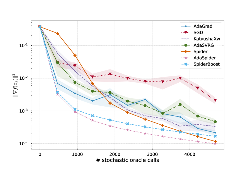
(a) MNIST

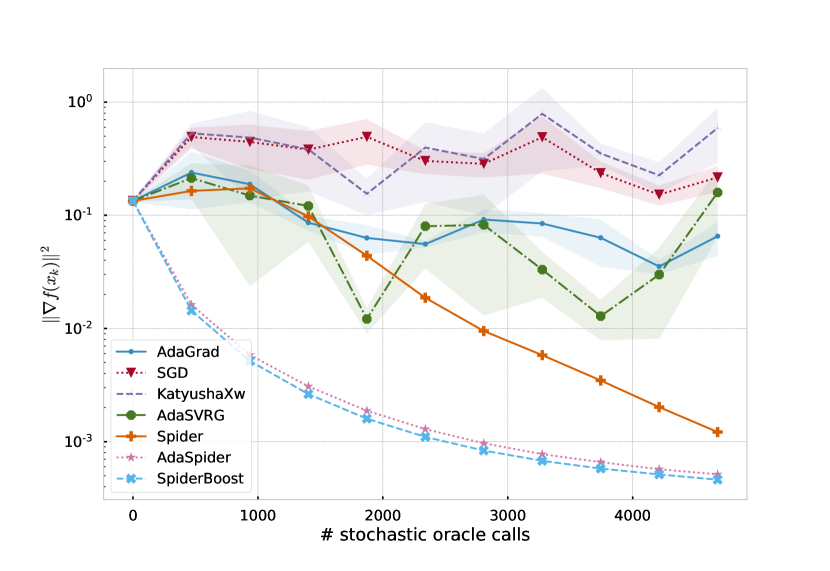
(b) FashionMNIST

Figure 2. Gradient norms throughout the epochs for image classification with neural networks (curves are averaged over 5 independent runs and the shaded region are the standard error).

	MNIST		FashionMNIST
	Batch Size $=32$, $c_{\text{init}}=0.03$		Batch Size $=128$, $c_{\text{init}}=0.01$
Algorithm	Parameters	Test Accuracy	Parameters	Test Accuracy
AdaGrad[16]	$\eta=0.01,\;\epsilon=10^{-4}$	$97.86$	$\eta=0.01,\;\epsilon=10^{-4}$	$86.19$
SGD[46]	$\eta=0.01$	$98.11$	$\eta=0.01$	$85.83$
KatyushaXw[3]	$\eta=0.005$	$97.93$	$\eta=0.01$	$86.27$
AdaSVRG[15]	$\eta=0.1$	$98.03$	$\eta=0.1$	$86.82$
Spider[19]	$\epsilon=0.01,\;L=100.0,\;n_{0}=1$	$97.53$	$\epsilon=0.01,\;L=50.0,\;n_{0}=1$	$82.22$
SpiderBoost[51, 42]	$L=200$	$97.01$	$L=120$	$84.42$
AdaSpider	$n=60000$	$97.49$	$n=60000$	$84.09$

Table 2. Algorithm parameters and test accuracies (average of 5 runs, in $\%$)

Observations:

We observe (Figure 2) that AdaSpider performs as well as other variance reduction methods in terms of minimizing the gradient norm. The key message here is that it does so without the need for extensive tuning. This diminished need for tuning is a welcome feature for deep learning optimization, but, often the true metric of interest is not the gradient norm, but the accuracy on unseen data, and on this metric variance reduction schemes are not yet competitive with simpler methods like SGD. With AdaSpider, the focus can go to finding the right initialization scheme and architecture to ensure good generalization without being distracted by other parameters like the step-size choice.

Appendix A Omitted Proofs

We first state two technical lemmas that have been extensively used in the analysis of adaptive methods, the proofs of which can be found in [31].

Lemma 6.

Let a sequence of non-negative real numbers $\alpha_{1},\ldots,\alpha_{T}\geq 0$ then

$$\sqrt{\sum_{t=1}^{T}\alpha_{t}}\leq\sum_{t=1}^{T}\frac{\alpha_{t}}{\sqrt{\sum_{s=1}^{t}\alpha_{s}}}$$

Lemma 7.

Let a sequence of non-negative real numbers $\alpha_{1},\ldots,\alpha_{T}\geq 0$ then

$$\sum_{t=1}^{T}\frac{\alpha_{t}}{1+\sum_{s=1}^{t}\alpha_{s}}\leq\log\left(1+\sum_{t=1}^{T}\alpha_{t}\right)$$

Lemma 1.

Define the gradient estimator at point $x$ as $\nabla_{x}:=\nabla f_{i}(x)-\nabla f_{i}(y)+\nabla_{y}$ where $i$ is sampled uniformly at random from $\{1,\ldots,n\}$. Then,

$$\mathbb{E}\left[\lVert\nabla_{x}-\nabla f(x)\rVert^{2}\right]\leq L^{2}\lVert x-y\rVert^{2}+\mathbb{E}\left[\lVert\nabla_{y}-\nabla f(y)\rVert^{2}\right]$$

Proof.

$$\mathbb{E}\left[\lVert\nabla_{x}-\nabla f(x)\rVert^{2}\right] = \mathbb{E}\left[\lVert\nabla f_{i}(x)-\nabla f_{i}(y)+\nabla_{y}-\nabla f(x)\rVert^{2}\right]$$

$$= \mathbb{E}\left[\lVert\nabla f_{i}(x)-\nabla f_{i}(y)+\nabla_{y}-\nabla f(x)+\nabla f(y)-\nabla f(y)\rVert^{2}\right]$$

$$= \mathbb{E}\left[\lVert\nabla f_{i}(x)-\nabla f_{i}(y)-\nabla f(x)+\nabla f(y)\rVert^{2}\right]$$

$$+ 2\cdot\mathbb{E}\left[\left\langle\nabla f_{i}(x)-\nabla f_{i}(y)-\nabla f(x)+\nabla f(y),\nabla_{y}-\nabla f(y)\right\rangle\right]$$

$$+ \mathbb{E}\left[\lVert\nabla_{y}-\nabla f(y)\rVert^{2}\right]$$

Notice that $\mathbb{E}\left[\nabla f_{i}(x)-\nabla f_{i}(y)-\nabla f(x)+\nabla f(y)\right]=0$ due to the fact that $i$ is selected uniformly at random in $\{1,\ldots,n\}$ and thus $\mathbb{E}\left[\nabla f_{i}(x)-\nabla f_{i}(y)\right]=\nabla f(x)-\nabla f(y)$. The latter implies that,

$$\mathbb{E}\left[\lVert\nabla_{x}-\nabla f(x)\rVert^{2}\right] = \mathbb{E}\left[\lVert\nabla f_{i}(x)-\nabla f_{i}(y)-\nabla f(x)+\nabla f(y)\rVert^{2}\right]+\mathbb{E}\left[\lVert\nabla_{y}-\nabla f(y)\rVert^{2}\right]$$

$$\leq \mathbb{E}\left[\lVert\nabla f_{i}(x)-\nabla f_{i}(y)\rVert^{2}\right]+\mathbb{E}\left[\lVert\nabla_{y}-\nabla f(y)\rVert^{2}\right]$$

$$\leq L^{2}\cdot\mathbb{E}\left[\lVert x-y\rVert^{2}\right]+\mathbb{E}\left[\lVert\nabla_{y}-\nabla f(y)\rVert^{2}\right]$$

where the first inequality follows by the identity $\mathbb{E}\left[\lVert X-\mathbb{E}\left[X\right]\rVert^{2}\right]=\mathbb{E}[\lVert X\rVert^{2}]-\lVert\mathbb{E}\left[X\right]\rVert^{2}$ and the second inequality by the smoothness of the function $f_{i}(x)$. ∎

Lemma 2.

Let $x_{0},x_{1},\ldots,x_{T}$ the points produced by Algorithm 1. Then,

$$\sum_{t=0}^{T-1}\lVert\nabla_{t}\rVert^{2}\leq\mathcal{O}\left(n^{2}T^{3}\cdot\left(\frac{L^{2}}{\beta_{0}^{2}}+\lVert\nabla f(x_{0})\rVert^{2}\right)\right)$$

Proof.

The selection of the step-size in Step $9$ of Algorithm 1 implies that $\lVert x_{t+1}-x_{t}\rVert^{2}=\lVert\gamma_{t}\nabla_{t}\rVert^{2}\leq 1/\beta_{0}^{2}$. Due to the fact that every $n$ iterations a full-gradient computation is performed, the estimator $\nabla_{t}:=\nabla f_{i_{t}}(x_{t})-\nabla f_{i_{t}}(x_{t-1})+\nabla_{t-1}$ can be equivalently written as

$$\nabla_{t}=\sum_{s=t-t~{}\mathrm{mod}~{}n+1}^{t}\left(\nabla f_{i_{s}}(x_{s})-\nabla f_{i_{s}}(x_{s-1})\right)+\nabla f(x_{t-t~{}\mathrm{mod}~{}n})$$

As a result,

$$\lVert\nabla_{t}\rVert^{2} = \lVert\sum_{s=t-t~{}\mathrm{mod}~{}n+1}^{t}\left(\nabla f_{i_{s}}(x_{s})-\nabla f_{i_{s}}(x_{s-1})\right)+\nabla f(x_{t-t~{}\mathrm{mod}~{}n})\rVert^{2}$$

$$\leq 2\cdot\lVert\sum_{s=t-t~{}\mathrm{mod}~{}n+1}^{t}\nabla f_{i_{s}}(x_{s})-\nabla f_{i_{s}}(x_{s-1})\rVert^{2}+2\cdot\lVert\nabla f(x_{t-t~{}\mathrm{mod}~{}n})\rVert^{2}$$

$$\leq 2n\cdot\sum_{s=t-t~{}\mathrm{mod}~{}n+1}^{t}\lVert\nabla f_{i_{s}}(x_{s})-\nabla f_{i_{s}}(x_{s-1})\rVert^{2}+2\cdot\lVert\nabla f(x_{t-t~{}\mathrm{mod}~{}n})\rVert^{2}$$

$$\leq 2nL^{2}\cdot\sum_{s=t-t~{}\mathrm{mod}~{}n+1}^{t}\lVert x_{s}-x_{s-1}\rVert^{2}+2\cdot\lVert\nabla f(x_{t-t~{}\mathrm{mod}~{}n})\rVert^{2}$$

$$\leq \frac{2L^{2}n^{2}}{\beta_{0}^{2}}+2\cdot\lVert\nabla f(x_{t-t~{}\mathrm{mod}~{}n})\rVert^{2}$$

Now, we want to upper bound $\lVert\nabla f(x_{t})\rVert$ for any $t\leq T$ with respect to the initial gradient norm. Using again the step-size selection $\gamma_{t}$ we get,

$$\lVert\nabla f(x_{t})\rVert =\lVert\nabla f(x_{t})-\nabla f(x_{0})+\nabla f(x_{0})\rVert$$

$$\leq\lVert\nabla f(x_{t})-\nabla f(x_{0})\rVert+\lVert\nabla f(x_{0})\rVert$$ (Triangular inequality)

$$\leq L\lVert x_{t}-x_{0}\rVert+\lVert\nabla f(x_{0})\rVert$$ (Smoothness)

$$\leq L\lVert x_{t}-x_{t-1}\rVert+L\lVert x_{t-1}-x_{0}\rVert+\lVert\nabla f(x_{0})\rVert$$ (Triangular inequality)

$$\leq L\sum_{i=1}^{t}\lVert x_{i}-x_{i-1}\rVert+\lVert\nabla f(x_{0})\rVert$$

$$\leq\frac{Lt}{\beta_{0}}+\lVert\nabla f(x_{0})\rVert$$

As a result,

$$\sum_{t=0}^{T-1}\lVert\nabla_{t}\rVert^{2} \leq\sum_{t=0}^{T-1}\left(\frac{2L^{2}n^{2}}{\beta_{0}^{2}}+2\cdot\lVert\nabla f(x_{t-t~{}\mathrm{mod}~{}n})\rVert^{2}\right)$$

$$\leq\frac{2L^{2}n^{2}}{\beta_{0}^{2}}T+2\sum_{t=0}^{T-1}\lVert\nabla f(x_{t})\rVert^{2}$$

$$\leq\frac{2L^{2}n^{2}}{\beta_{0}^{2}}T+2\sum_{t=0}^{T-1}(\frac{Lt}{\beta_{0}}+\lVert\nabla f(x_{0})\rVert)^{2}$$

$$=\frac{2L^{2}n^{2}}{\beta_{0}^{2}}T+2\sum_{t=0}^{T-1}\left(\frac{L^{2}t^{2}}{\beta_{0}^{2}}+2\frac{Lt}{\beta_{0}}\lVert\nabla f(x_{0})\rVert+\lVert\nabla f(x_{0})\rVert^{2}\right)$$

$$\leq\frac{2L^{2}n^{2}}{\beta_{0}^{2}}T+\frac{2L^{2}T^{3}}{\beta_{0}^{2}}+\frac{4LT^{2}\lVert\nabla f(x_{0})\rVert}{\beta_{0}}+2T\lVert\nabla f(x_{0})\rVert^{2}$$

∎

Lemma 3.

Let $x_{0},x_{1}\ldots,x_{T}$ the sequence of points produced by Algorithm 1. Then,

$$\sum_{t=0}^{T-1}\mathbb{E}\left[\lVert\nabla_{t}-\nabla f(x_{t})\rVert^{2}\right]\leq\mathcal{O}\left(\frac{Ln^{1/4}}{\beta_{0}}\sqrt{\log\left(1+nT\cdot\left(\frac{L}{\beta_{0}G_{0}}+\frac{\lVert\nabla f(x_{0})\rVert}{G_{0}}\right)\right)}\right).$$

Proof.

$$\mathbb{E}\left[\sum_{t=0}^{T-1}\lVert\nabla_{t}-\nabla f(x_{t})\rVert\right] = \mathbb{E}\left[\sqrt{\left(\sum_{t=0}^{T-1}\lVert\nabla_{t}-\nabla f(x_{t})\rVert\right)^{2}}\right]$$

$$\leq \sqrt{\mathbb{E}\left[\left(\sum_{t=0}^{T-1}\lVert\nabla_{t}-\nabla f(x_{t})\rVert\right)^{2}\right]}$$ (Jensen’s ineq.)

$$\leq \sqrt{T}\cdot\sqrt{\mathbb{E}\left[\sum_{t=0}^{T-1}\lVert\nabla_{t}-\nabla f(x_{t})\rVert^{2}\right]}$$

where the last inequality follows by the fact that $\lVert\sum_{t=0}^{T-1}y_{t}\rVert^{2}\leq T\cdot\sum_{t=0}^{T-1}\lVert y_{t}\rVert^{2}$. By applying Lemma 1 to the estimator $\nabla_{t}:=\nabla f_{i_{t}}(x_{t})-\nabla f_{i_{t}}(x_{t-1})+\nabla_{t-1}$ we get,

$$\mathbb{E}\left[\lVert\nabla_{t}-\nabla f(x_{t})\rVert^{2}\right] \leq L^{2}\mathbb{E}\left[\lVert x_{t}-x_{t-1}\rVert^{2}\right]+\mathbb{E}\left[\lVert\nabla_{t-1}-\nabla f(x_{t-1})\rVert^{2}\right]$$

$$\leq L^{2}\mathbb{E}\left[\gamma^{2}_{t-1}\lVert\nabla_{t-1}\rVert^{2}\right]+\mathbb{E}\left[\lVert\nabla_{t-1}-\nabla f(x_{t-1})\rVert^{2}\right]$$

$$\leq L^{2}\mathbb{E}\left[\gamma^{2}_{t-1}\lVert\nabla_{t-1}\rVert^{2}\right]+\ldots+\mathbb{E}\left[\lVert\nabla_{t-(t~{}\mathrm{mod}~{}n)}-\nabla f(x_{t-(t~{}\mathrm{mod}~{}n})\rVert^{2}\right]$$

$$= \sum_{\tau=t-(t~{}\text{mod }n)+1}^{t-1}L^{2}\mathbb{E}\left[\gamma^{2}_{\tau}\cdot\lVert\nabla_{\tau}\rVert^{2}\right]$$

where the last equality follows by the fact that $\mathbb{E}\left[\lVert\nabla_{t-(t~{}\mathrm{mod}~{}n)}-\nabla f(x_{t-(t~{}\mathrm{mod}~{}n})\rVert^{2}\right]=0$ (see Step $3$ of Algorithm 1). As explained in Section 3, by a telescoping summation over $t$ we get that

$$\sum_{t=0}^{T-1}\mathbb{E}\left[\lVert\nabla_{t}-\nabla f(x_{t})\rVert^{2}\right]\leq L^{2}n\cdot\mathbb{E}\left[\sum_{t=0}^{T-1}\gamma_{t}^{2}\cdot\lVert\nabla_{t}\rVert^{2}\right].$$

Now as discussed in Section 3, using the step-size selection $\gamma_{t}$ of Algorithm 1 we can provide a bound on the total variance $\mathbb{E}\left[\lVert\nabla_{t}-\nabla f(x_{t})\rVert^{2}\right]$

$$\sum_{t=0}^{T-1}\mathbb{E}\left[\lVert\nabla_{t}-\nabla f(x_{t})\rVert^{2}\right] \leq L^{2}n~{}\mathbb{E}\left[\sum_{t=0}^{T-1}\gamma_{t}^{2}\cdot\lVert\nabla_{t}\rVert^{2}\right]$$

$$= \frac{L^{2}\sqrt{n}}{\beta_{0}^{2}}~{}\mathbb{E}\left[\sum_{t=0}^{T-1}\frac{\lVert\nabla_{t}\rVert^{2}}{\sqrt{n}G_{0}^{2}+\sum_{s=0}^{t}\lVert\nabla_{s}\rVert^{2}}\right]$$

$$\leq \frac{L^{2}\sqrt{n}}{\beta_{0}^{2}}\log\left(1+\mathbb{E}\left[{\sum_{t=0}^{T-1}\lVert\nabla_{t}\rVert^{2}/G_{0}^{2}}\right]\right)$$

$$\leq \frac{L^{2}\sqrt{n}}{\beta_{0}^{2}}\cdot\mathcal{O}\left(\log\left(1+nT\cdot\left(\frac{L}{\beta_{0}G_{0}}+\frac{\lVert\nabla f(x_{0})\rVert}{G_{0}}\right)\right)\right)$$

where the second inequality follows by Lemma 7 and the third inequality by Lemma 2. Putting everything together we get

$$\frac{1}{T}\mathbb{E}\left[\sum_{t=0}^{T-1}\lVert\nabla_{t}-\nabla f(x_{t})\rVert\right]\leq\frac{Ln^{1/4}}{\beta_{0}\sqrt{T}}\cdot\mathcal{O}\left(\sqrt{\log\left(1+nT\cdot\left(\frac{L}{\beta_{0}G_{0}}+\frac{\lVert\nabla f(x_{0})\rVert}{G_{0}}\right)\right)}\right)$$

∎

Lemma 4.

Let $x_{0},x_{1},\ldots,x_{T-1}$ the sequence of points produced by Algorithm 1 and $\Delta_{0}:=f(x_{0})-f^{\ast}$. Then,

$$\mathbb{E}\left[\sum_{t=0}^{T-1}\lVert\nabla_{t}\rVert\right]\leq O\left(\Delta_{0}\cdot\beta_{0}+G_{0}+\frac{L}{\beta_{0}}\log\left(1+nT\cdot\frac{L+\lVert\nabla f(x_{0})\rVert}{G_{0}}\right)+\beta_{0}\cdot\mathbb{E}\left[\sum_{t=0}^{T-1}\gamma_{t}\lVert\nabla f(x_{t})-\nabla_{t}\rVert^{2}\right]\right)\cdot n^{1/4}\sqrt{T}.$$

Proof.

Let $\mathcal{F}_{t}$ denote the filtration at round $t$ i.e. all the random choices $\{i_{0},\ldots,i_{t}\}$ and the initial point $x_{0}$. By the smoothness of $f$ we get that,

$$\mathbb{E}\left[f(x_{t+1})~{}|~{}\mathcal{F}_{t}\right] \leq \mathbb{E}\left[f(x_{t})+\nabla f(x_{t})^{\top}(x_{t+1}-x_{t})+\frac{L}{2}\lVert x_{t}-x_{t+1}\rVert^{2}~{}|~{}\mathcal{F}_{t}\right]$$

$$= \mathbb{E}\left[f(x_{t})-\gamma_{t}\nabla_{t}^{\top}\nabla f(x_{t})+\frac{L}{2}\gamma_{t}^{2}\lVert\nabla_{t}\rVert^{2}~{}|~{}\mathcal{F}_{t}\right]$$

$$\leq \mathbb{E}\left[f(x_{t})+\frac{\gamma_{t}}{2}\lVert\nabla_{t}-\nabla f(x_{t})\rVert^{2}-\frac{\gamma_{t}}{2}(1-L\gamma_{t})\lVert\nabla_{t}\rVert^{2}~{}|~{}\mathcal{F}_{t}\right]$$

Thus,

$$\mathbb{E}\left[\gamma_{t}\cdot\lVert\nabla_{t}\rVert^{2}\right]\leq 2\mathbb{E}\left[f(x_{t})-f(x_{t+1})\right]+\mathbb{E}\left[L\gamma_{t}^{2}\cdot\lVert\nabla_{t}\rVert^{2}\right]+\beta_{0}\cdot\mathbb{E}\left[\gamma_{t}\cdot\lVert\nabla f(x_{t})-\nabla_{t}\rVert^{2}\right].$$

and by summing from $t=0$ to $T-1$ we get,

$$\sum_{t=0}^{T-1}\mathbb{E}\left[\gamma_{t}\cdot\lVert\nabla_{t}\rVert^{2}\right]\leq 2\Delta_{0}+\mathbb{E}\left[\sum_{t=0}^{T-1}L\gamma_{t}^{2}\cdot\lVert\nabla_{t}\rVert^{2}\right]+\mathbb{E}\left[\sum_{t=0}^{T-1}\gamma_{t}\cdot\lVert\nabla f(x_{t})-\nabla_{t}\rVert^{2}\right]$$

Using the fact that $\gamma_{t}:=n^{-1/4}\beta_{0}^{-1}\left(n^{1/2}G_{0}^{2}+\sum_{s=0}^{t}\lVert\nabla_{s}\rVert^{2}\right)^{-1/2}$ on the second summation term,

$$\mathbb{E}\left[\sum_{t=0}^{T-1}\gamma_{t}\cdot\lVert\nabla_{t}\rVert^{2}\right] \leq 2\Delta_{0}+\mathbb{E}\left[\sum_{t=0}^{T-1}L\gamma_{t}^{2}\cdot\lVert\nabla_{t}\rVert^{2}\right]+\mathbb{E}\left[\sum_{t=0}^{T-1}\gamma_{t}\cdot\lVert\nabla f(x_{t})-\nabla_{t}\rVert^{2}\right]$$

$$\leq 2\Delta_{0}+\frac{L}{\beta_{0}^{2}}\cdot\mathbb{E}\left[\sum_{t=0}^{T-1}\frac{\lVert\nabla_{t}\rVert^{2}}{\sqrt{n}G_{0}^{2}+\sum_{s=0}^{t}\lVert\nabla_{t}\rVert^{2}}\right]$$

$$+ \mathbb{E}\left[\sum_{t=0}^{T-1}\gamma_{t}\cdot\lVert\nabla f(x_{t})-\nabla_{t}\rVert^{2}\right]$$

$$\leq 2\Delta_{0}+\frac{L}{\beta_{0}^{2}}\cdot\mathcal{O}\left(\log\left(1+nT\cdot\left(\frac{L}{\beta_{0}G_{0}}+\frac{\lVert\nabla f(x_{0})\rVert}{G_{0}}\right)\right)\right)+\mathbb{E}\left[\sum_{t=0}^{T-1}\gamma_{t}\cdot\lVert\nabla f(x_{t})-\nabla_{t}\rVert^{2}\right]$$

Using again the definition of the step-size $\gamma_{t}:=n^{-1/4}\beta_{0}^{-1}\left(n^{1/2}G_{0}^{2}+\sum_{s=0}^{t}\lVert\nabla_{s}\rVert^{2}\right)^{-1/2}$ we lower bound the right-hand side as follows,

$$\mathbb{E}\left[\sum_{t=0}^{T-1}\gamma_{t}\cdot\lVert\nabla_{t}\rVert^{2}\right] \geq \mathbb{E}\left[\frac{\sum_{t=0}^{T-1}\lVert\nabla_{t}\rVert^{2}}{n^{1/4}\beta_{0}\sqrt{n^{1/2}G_{0}^{2}+\sum_{t=0}^{T-1}\lVert\nabla_{t}\rVert^{2}}}\right]$$

$$\geq \frac{G_{0}}{\beta_{0}}\cdot\mathbb{E}\left[\frac{\sum_{t=0}^{T-1}\lVert\nabla_{t}\rVert^{2}/\sqrt{n}G_{0}^{2}}{\sqrt{1+\sum_{t=0}^{T-1}\lVert\nabla_{t}\rVert^{2}/\sqrt{n}G_{0}^{2}}}\right]$$

$$\geq \frac{G_{0}}{\beta_{0}}\cdot\left(\mathbb{E}\left[\sqrt{\sum_{t=0}^{T-1}\lVert\nabla_{t}\rVert^{2}/\sqrt{n}G_{0}^{2}}\right]-1\right)$$

$$\geq \frac{1}{\beta_{0}n^{1/4}\sqrt{T}}\mathbb{E}\left[\sum_{t=0}^{T-1}\lVert\nabla_{t}\rVert\right]-\frac{G_{0}}{\beta_{0}}$$

By putting everything together we get,

$$\mathbb{E}\left[\sum_{t=0}^{T-1}\lVert\nabla_{t}\rVert\right] \leq O\left(\Delta_{0}\cdot\beta_{0}+G_{0}+\frac{L}{\beta_{0}}\log\left(1+nT\cdot\left(\frac{L}{\beta_{0}G_{0}}+\frac{\lVert\nabla f(x_{0})\rVert}{G_{0}}\right)\right)\right)$$

$$+ \mathcal{O}\left(\beta_{0}\cdot\mathbb{E}\left[\sum_{t=0}^{T-1}\gamma_{t}\lVert\nabla f(x_{t})-\nabla_{t}\rVert^{2}\right]\right)\cdot n^{1/4}\sqrt{T}.$$

∎

Lemma 5.

Let $x_{0},x_{1},\ldots,x_{T-1}$ the sequence of points produced by Algorithm 1. Then,

$$\mathbb{E}\left[\sum_{t=0}^{T-1}\gamma_{t}\cdot\lVert\nabla_{t}-\nabla f(x_{t})\rVert^{2}\right]\leq L^{2}n\cdot\mathbb{E}\left[\sum_{t=0}^{T-1}\gamma_{t}^{3}\cdot\lVert\nabla_{t}\rVert^{2}\right]$$

Proof.

Let $\mathcal{F}_{t}$ denotes the filtration at round $t$ i.e. all the random choices $\{i_{0},\ldots,i_{t}\}$ and the initial point $x_{0}$. At first notice that by the definition of $\gamma_{t}$ in Step $9$ of Algorithm 1, $\gamma_{t}\leq\gamma_{t-1}$, which we have to do to circumvent non-measurability issues, and thus

$$\mathbb{E}\left[\gamma_{t}\lVert\nabla_{t}-\nabla f(x_{t})\rVert^{2}~{}|~{}\mathcal{F}_{t-1}\right]\leq\mathbb{E}\left[\gamma_{t-1}\cdot\lVert\nabla_{t}-\nabla f(x_{t})\rVert^{2}~{}|~{}\mathcal{F}_{t-1}\right]$$

Up next we derive a bound on $\mathbb{E}\left[\gamma_{t-1}\cdot\lVert\nabla_{t}-\nabla f(x_{t})\rVert^{2}~{}|~{}\mathcal{F}_{t-1}\right]$ using similar arguments with the ones used in Lemma 3. Notice that $\gamma_{t-1}$ is $\mathcal{F}_{t-1}$-measurable, hence we can treat in independent of the conditional expectation.

$$\mathbb{E}\left[\gamma_{t-1}\lVert\nabla_{t}-\nabla f(x_{t})\rVert^{2}~{}|~{}\mathcal{F}_{t-1}\right]$$

$$= \gamma_{t-1}\mathbb{E}\left[\lVert\nabla f_{i_{t}}(x_{t})-\nabla f_{i_{t}}(x_{t-1})-\nabla f(x_{t})+\nabla f(x_{t-1})+(\nabla_{t-1}-\nabla f(x_{t-1}))\rVert^{2}~{}|~{}\mathcal{F}_{t-1}\right]$$

$$= \gamma_{t-1}\mathbb{E}\left[\lVert\nabla f_{i_{t}}(x_{t})-\nabla f_{i_{t}}(x_{t-1})-\nabla f(x_{t})+\nabla f(x_{t-1})\rVert^{2}~{}|~{}\mathcal{F}_{t-1}\right]$$

$$+ \gamma_{t-1}\underbrace{\mathbb{E}\left[(\nabla f_{i_{t}}(x_{t})-\nabla f_{i_{t}}(x_{t-1})-\nabla f(x_{t})+\nabla f(x_{t-1}))^{\top}(\nabla_{t-1}-\nabla f(x_{t-1}))~{}|~{}\mathcal{F}_{t-1}\right]}_{0}$$

$$+ \gamma_{t-1}\mathbb{E}\left[\lVert\nabla_{t-1}-\nabla f(x_{t-1})\rVert^{2}~{}|~{}\mathcal{F}_{t-1}\right]$$

$$= \gamma_{t-1}\mathbb{E}\left[\lVert\nabla f_{i_{t}}(x_{t})-\nabla f_{i_{t}}(x_{t-1})\rVert^{2}~{}|~{}\mathcal{F}_{t-1}\right]+\gamma_{t-1}\mathbb{E}\left[\lVert\nabla_{t-1}-\nabla f(x_{t-1})\rVert^{2}~{}|~{}\mathcal{F}_{t-1}\right]$$

$$\leq L^{2}\gamma_{t-1}\mathbb{E}\left[\lVert x_{t}-x_{t-1}\rVert^{2}~{}|~{}\mathcal{F}_{t-1}\right]+\gamma_{t-1}\mathbb{E}\left[\lVert\nabla_{t-1}-\nabla f(x_{t-1})\rVert^{2}~{}|~{}\mathcal{F}_{t-1}\right]$$

$$= L^{2}\gamma^{3}_{t-1}\mathbb{E}\left[\lVert\nabla_{t-1}\rVert^{2}~{}|~{}\mathcal{F}_{t-1}\right]+\gamma_{t-1}\mathbb{E}\left[\lVert\nabla_{t-1}-\nabla f(x_{t-1})\rVert^{2}~{}|~{}\mathcal{F}_{t-1}\right]$$

Taking full expectation over all randomness and by the law of total expctation, we get that,

$$\mathbb{E}\left[\gamma_{t}\lVert\nabla_{t}-\nabla f(x_{t})\rVert^{2}\right]\leq L^{2}\mathbb{E}\left[\gamma^{3}_{t-1}\lVert\nabla_{t-1}\rVert^{2}\right]+\mathbb{E}\left[\gamma_{t-1}\lVert\nabla_{t-1}-\nabla f(x_{t-1})\rVert^{2}\right]$$

Due to the fact that $\mathbb{E}\left[\lVert\nabla_{t}-\nabla f(x_{t})\rVert\right]=0$ for $t~{}\mathrm{mod}~{}n==0$ we get that

$$\mathbb{E}\left[\gamma_{t}\cdot\lVert\nabla_{t}-\nabla f(x_{t})\rVert^{2}\right]\leq L^{2}\mathbb{E}\left[\sum_{s=t-t~{}\mathrm{mod}~{}n}^{t-1}\gamma_{s}^{3}\lVert\nabla_{s}\rVert^{2}\right]$$

and thus

$$\mathbb{E}\left[\sum_{t=0}^{T-1}\gamma_{t}\cdot\lVert\nabla_{t}-\nabla f(x_{t})\rVert^{2}\right]\leq L^{2}n\cdot\mathbb{E}\left[\sum_{t=0}^{T-1}\gamma_{t}^{3}\lVert\nabla_{t}\rVert^{2}\right]$$

∎

Theorem 1.

Let $x_{0},x_{1},\ldots,x_{T-1}$ be the sequence of points produced by Algorithm 1 in case $f(\cdot)$ is $L$-smooth. Let us also define $\Delta_{0}:=f(x_{0})-f^{\ast}$. Then,

$$\frac{1}{T}\sum_{t=0}^{T-1}\mathbb{E}\left[\lVert\nabla f(x_{t})\rVert\right]\leq O\left(n^{1/4}\cdot\frac{\Delta_{0}\cdot\beta_{0}+G_{0}+L/\beta_{0}+L^{2}/\beta_{0}^{2}G_{0}}{\sqrt{T}}\cdot\log\left(1+nT\cdot\left(\frac{L}{\beta_{0}G_{0}}+\frac{\lVert\nabla f(x_{0})\rVert}{G_{0}}\right)\right)\right)$$

Overall, Algorithm 1 with $\beta_{0}:=1$ and $G_{0}:=1$ needs at most $\tilde{O}\left(n+\sqrt{n}\cdot\frac{\Delta_{0}^{2}+L^{4}}{\epsilon^{2}}\right)$ oracle calls to reach an $\epsilon$-stationary point.

Proof of Theorem 1.

By the triangle inequality we get that

$$\mathbb{E}\left[\sum_{t=0}^{T-1}\lVert\nabla f(x_{t})\rVert\right]\leq\mathbb{E}\left[\sum_{t=0}^{T-1}\lVert\nabla_{t}\rVert\right]+\mathbb{E}\left[\sum_{t=0}^{T-1}\lVert\nabla f(x_{t})-\nabla_{t}\rVert\right]$$

Using the bounds obtained in Lemma 3 and Lemma 4 we get that,

$$\mathbb{E}\left[\sum_{t=0}^{T-1}\lVert\nabla f(x_{t})\rVert\right] \leq \tilde{O}\left(\Delta_{0}\cdot\beta_{0}+G_{0}+\frac{L}{\beta_{0}}\right)n^{1/4}\sqrt{T}$$

$$+ \beta_{0}\cdot\mathbb{E}\left[\sum_{t=0}^{T-1}\gamma_{t}\lVert\nabla f(x_{t})-\nabla_{t}\rVert^{2}\right]n^{1/4}\sqrt{T}$$

Then by Lemma 5 we get that,

$$\mathbb{E}\left[\sum_{t=0}^{T-1}\lVert\nabla f(x_{t})\rVert\right] \leq \tilde{O}\left(\Delta_{0}\cdot\beta_{0}+G_{0}+\frac{L}{\beta_{0}}\right)n^{1/4}\sqrt{T}$$

$$+ \beta_{0}\cdot\underbrace{n^{5/4}\sqrt{T}L^{2}\cdot\mathbb{E}\left[\sum_{t=0}^{T-1}\gamma_{t}^{3}\lVert\nabla_{t}\rVert^{2}\right]}_{\mathrm{(A)}}$$

Substituing the selection of $\gamma_{t}$ in term $(\mathrm{A})$ we get,

$$\beta_{0}\sqrt{T}L^{2}\cdot\mathbb{E}\left[\sum_{t=0}^{T-1}n^{5/4}\gamma_{t}^{3}\lVert\nabla_{t}\rVert^{2}\right] = \frac{\sqrt{T}L^{2}}{\beta_{0}^{2}}\cdot\mathbb{E}\left[\sum_{t=0}^{T-1}\frac{n^{5/4}}{n^{3/4}\sqrt{n^{1/2}G_{0}^{2}+\sum_{s=0}^{t}\lVert\nabla_{t}\rVert^{2}}}\cdot\frac{\lVert\nabla_{t}\rVert^{2}}{{n}^{1/2}G_{0}^{2}+\sum_{s=0}^{t}\lVert\nabla_{t}\rVert^{2}}\right]$$

$$\leq \frac{\sqrt{T}L^{2}}{\beta_{0}^{2}G_{0}}\cdot\mathbb{E}\left[\sum_{t=0}^{T-1}\frac{n^{5/4}}{n^{3/4}\sqrt{n^{1/2}}}\cdot\frac{\lVert\nabla_{t}\rVert^{2}/G_{0}^{2}}{{n}^{1/2}+\sum_{s=0}^{t}\lVert\nabla_{t}\rVert^{2}/G_{0}^{2}}\right]$$

$$\leq \frac{\sqrt{T}L^{2}}{\beta_{0}^{2}G_{0}}\cdot n^{1/4}\cdot\mathbb{E}\left[\sum_{t=0}^{T-1}\frac{\lVert\nabla_{t}\rVert^{2}/G_{0}^{2}}{1+\sum_{s=0}^{t}\lVert\nabla_{t}\rVert^{2}/G_{0}^{2}}\right]$$

$$\leq \frac{\sqrt{T}L^{2}}{\beta_{0}^{2}G_{0}}\cdot n^{1/4}\cdot\mathcal{O}\left(\log\left(1+nT\cdot\left(\frac{L}{\beta_{0}G_{0}}+\frac{\lVert\nabla f(x_{0})\rVert}{G_{0}}\right)\right)\right)$$

where the forth inequality follows by Lemma 7 and the last by Lemma 2. Theorem 1 then follows by dividing both sides with $T$. ∎

References

• Allen-Zhu [2017a] Zeyuan Allen-Zhu. Natasha: Faster non-convex stochastic optimization via strongly non-convex parameter, 2017a. URL https://arxiv.org/abs/1702.00763.
• Allen-Zhu [2017b] Zeyuan Allen-Zhu. Katyusha: The first direct acceleration of stochastic gradient methods. In Proceedings of the 49th Annual ACM SIGACT Symposium on Theory of Computing, STOC 2017, page 1200–1205. Association for Computing Machinery, 2017b.
• Allen-Zhu [2018] Zeyuan Allen-Zhu. Katyusha X: Practical Momentum Method for Stochastic Sum-of-Nonconvex Optimization. In Proceedings of the 35th International Conference on Machine Learning, ICML ’18, 2018. Full version available at http://arxiv.org/abs/1802.03866.
• Allen-Zhu and Hazan [2016] Zeyuan Allen-Zhu and Elad Hazan. Variance reduction for faster non-convex optimization. In Proceedings of the 33rd International Conference on International Conference on Machine Learning - Volume 48, ICML’16, page 699–707. JMLR.org, 2016.
• Antonakopoulos et al. [2021a] Kimon Antonakopoulos, Elena Veronica Belmega, and Panayotis Mertikopoulos. Adaptive extra-gradient methods for min-max optimization and games. In 9th International Conference on Learning Representations, ICLR 2021, Virtual Event, Austria, May 3-7, 2021. OpenReview.net, 2021a.
• Antonakopoulos et al. [2021b] Kimon Antonakopoulos, Thomas Pethick, Ali Kavis, Panayotis Mertikopoulos, and Volkan Cevher. Sifting through the noise: Universal first-order methods for stochastic variational inequalities. In Marc’Aurelio Ranzato, Alina Beygelzimer, Yann N. Dauphin, Percy Liang, and Jennifer Wortman Vaughan, editors, Advances in Neural Information Processing Systems 34: Annual Conference on Neural Information Processing Systems 2021, NeurIPS 2021, December 6-14, 2021, virtual, pages 13099–13111, 2021b.
• Arjevani et al. [2019] Yossi Arjevani, Yair Carmon, John C. Duchi, Dylan J. Foster, Nathan Srebro, and Blake E. Woodworth. Lower bounds for non-convex stochastic optimization. CoRR, abs/1912.02365, 2019.
• Barzilai and Borwein [1988] Jonathan Barzilai and Jonathan M. Borwein. Two-Point Step Size Gradient Methods. IMA Journal of Numerical Analysis, 8(1):141–148, 01 1988. ISSN 0272-4979. doi: 10.1093/imanum/8.1.141. URL https://doi.org/10.1093/imanum/8.1.141.
• Bridle [1989] John Bridle. Training stochastic model recognition algorithms as networks can lead to maximum mutual information estimation of parameters. Advances in neural information processing systems, 2, 1989.
• Bridle [1990] John S Bridle. Probabilistic interpretation of feedforward classification network outputs, with relationships to statistical pattern recognition. In Neurocomputing, pages 227–236. Springer, 1990.
• Clevert et al. [2016] Djork-Arné Clevert, Thomas Unterthiner, and Sepp Hochreiter. Fast and accurate deep network learning by exponential linear units (elus). In Yoshua Bengio and Yann LeCun, editors, 4th International Conference on Learning Representations, ICLR 2016, San Juan, Puerto Rico, May 2-4, 2016, Conference Track Proceedings, 2016. URL http://arxiv.org/abs/1511.07289.
• Cutkosky and Orabona [2019] Ashok Cutkosky and Francesco Orabona. Momentum-based variance reduction in non-convex sgd. In H. Wallach, H. Larochelle, A. Beygelzimer, F. d'Alché-Buc, E. Fox, and R. Garnett, editors, Advances in Neural Information Processing Systems, volume 32. Curran Associates, Inc., 2019. URL https://proceedings.neurips.cc/paper/2019/file/b8002139cdde66b87638f7f91d169d96-Paper.pdf.
• Defazio et al. [2014] Aaron Defazio, Francis Bach, and Simon Lacoste-Julien. Saga: A fast incremental gradient method with support for non-strongly convex composite objectives. In Z. Ghahramani, M. Welling, C. Cortes, N. Lawrence, and K. Q. Weinberger, editors, Advances in Neural Information Processing Systems, volume 27. Curran Associates, Inc., 2014.
• Deng et al. [2009] Jia Deng, Wei Dong, Richard Socher, Li-Jia Li, Kai Li, and Li Fei-Fei. Imagenet: A large-scale hierarchical image database. In 2009 IEEE Conference on Computer Vision and Pattern Recognition, pages 248–255, 2009. doi: 10.1109/CVPR.2009.5206848.
• Dubois-Taine et al. [2021] Benjamin Dubois-Taine, Sharan Vaswani, Reza Babanezhad, Mark Schmidt, and Simon Lacoste-Julien. SVRG meets adagrad: Painless variance reduction. CoRR, abs/2102.09645, 2021. URL https://arxiv.org/abs/2102.09645.
• Duchi et al. [2011] John Duchi, Elad Hazan, and Yoram Singer. Adaptive subgradient methods for online learning and stochastic optimization. Journal of Machine Learning Research, 12(Jul):2121–2159, 2011.
• Ene et al. [2021] Alina Ene, Huy L. Nguyen, and Adrian Vladu. Adaptive gradient methods for constrained convex optimization and variational inequalities. In Thirty-Fifth AAAI Conference on Artificial Intelligence, AAAI 2021, Thirty-Third Conference on Innovative Applications of Artificial Intelligence, IAAI 2021, The Eleventh Symposium on Educational Advances in Artificial Intelligence, EAAI 2021, Virtual Event, February 2-9, 2021, pages 7314–7321. AAAI Press, 2021.
• Fang et al. [2018a] Cong Fang, Chris Junchi Li, Zhouchen Lin, and Tong Zhang. SPIDER: near-optimal non-convex optimization via stochastic path-integrated differential estimator. In Samy Bengio, Hanna M. Wallach, Hugo Larochelle, Kristen Grauman, Nicolò Cesa-Bianchi, and Roman Garnett, editors, Advances in Neural Information Processing Systems 31: Annual Conference on Neural Information Processing Systems 2018, NeurIPS 2018, December 3-8, 2018, Montréal, Canada, pages 687–697, 2018a.
• Fang et al. [2018b] Cong Fang, Chris Junchi Li, Zhouchen Lin, and Tong Zhang. Spider: Near-optimal non-convex optimization via stochastic path-integrated differential estimator. In S. Bengio, H. Wallach, H. Larochelle, K. Grauman, N. Cesa-Bianchi, and R. Garnett, editors, Advances in Neural Information Processing Systems, volume 31. Curran Associates, Inc., 2018b. URL https://proceedings.neurips.cc/paper/2018/file/1543843a4723ed2ab08e18053ae6dc5b-Paper.pdf.
• Faw et al. [2022] Matthew Faw, Isidoros Tziotis, Constantine Caramanis, Aryan Mokhtari, Sanjay Shakkottai, and Rachel Ward. The power of adaptivity in SGD: self-tuning step sizes with unbounded gradients and affine variance. In Po-Ling Loh and Maxim Raginsky, editors, Conference on Learning Theory, 2-5 July 2022, London, UK, volume 178 of Proceedings of Machine Learning Research, pages 313–355. PMLR, 2022.
• Gómez et al. [2020] Fabian Latorre Gómez, Paul Rolland, and Volkan Cevher. Lipschitz constant estimation of neural networks via sparse polynomial optimization. In 8th International Conference on Learning Representations, ICLR 2020, Addis Ababa, Ethiopia, April 26-30, 2020. OpenReview.net, 2020.
• He et al. [2015] Kaiming He, Xiangyu Zhang, Shaoqing Ren, and Jian Sun. Delving deep into rectifiers: Surpassing human-level performance on imagenet classification. In Proceedings of the IEEE international conference on computer vision, pages 1026–1034, 2015.
• Hsieh et al. [2021] Yu-Guan Hsieh, Kimon Antonakopoulos, and Panayotis Mertikopoulos. Adaptive learning in continuous games: Optimal regret bounds and convergence to nash equilibrium. In Mikhail Belkin and Samory Kpotufe, editors, Conference on Learning Theory, COLT 2021, 15-19 August 2021, Boulder, Colorado, USA, volume 134 of Proceedings of Machine Learning Research, pages 2388–2422. PMLR, 2021.
• Johnson and Zhang [2013] Rie Johnson and Tong Zhang. Accelerating stochastic gradient descent using predictive variance reduction. In Proceedings of the 26th International Conference on Neural Information Processing Systems - Volume 1, NIPS’13, page 315–323. Curran Associates Inc., 2013.
• Joulani et al. [2020] Pooria Joulani, Anant Raj, Andras Gyorgy, and Csaba Szepesvari. A simpler approach to accelerated optimization: iterative averaging meets optimism. In Hal Daumé III and Aarti Singh, editors, Proceedings of the 37th International Conference on Machine Learning, volume 119 of Proceedings of Machine Learning Research, pages 4984–4993. PMLR, 13–18 Jul 2020. URL https://proceedings.mlr.press/v119/joulani20a.html.
• Kavis et al. [2019] Ali Kavis, Kfir Y. Levy, Francis Bach, and Volkan Cevher. Unixgrad: A universal, adaptive algorithm with optimal guarantees for constrained optimization. In H. Wallach, H. Larochelle, A. Beygelzimer, F. d’Alché Buc, E. Fox, and R. Garnett, editors, Advances in Neural Information Processing Systems 32, pages 6260–6269. Curran Associates, Inc., 2019.
• Kavis et al. [2022] Ali Kavis, Kfir Yehuda Levy, and Volkan Cevher. High probability bounds for a class of nonconvex algorithms with adagrad stepsize. CoRR, abs/2204.02833, 2022.
• Lan et al. [2019a] Guanghui Lan, Zhize Li, and Yi Zhou. A unified variance-reduced accelerated gradient method for convex optimization. In Hanna M. Wallach, Hugo Larochelle, Alina Beygelzimer, Florence d’Alché-Buc, Emily B. Fox, and Roman Garnett, editors, Advances in Neural Information Processing Systems 32: Annual Conference on Neural Information Processing Systems 2019, NeurIPS 2019, December 8-14, 2019, Vancouver, BC, Canada, pages 10462–10472, 2019a.
• Lan et al. [2019b] Guanghui Lan, Zhize Li, and Yi Zhou. A unified variance-reduced accelerated gradient method for convex optimization, 2019b.
• Lecun et al. [1998] Y. Lecun, L. Bottou, Y. Bengio, and P. Haffner. Gradient-based learning applied to document recognition. Proceedings of the IEEE, 86(11):2278–2324, 1998. doi: 10.1109/5.726791.
• Levy et al. [2018] Kfir Y Levy, Alp Yurtsever, and Volkan Cevher. Online adaptive methods, universality and acceleration. In Neural and Information Processing Systems (NeurIPS), December 2018.
• Levy et al. [2021] Kfir Yehuda Levy, Ali Kavis, and Volkan Cevher. STORM+: Fully adaptive SGD with recursive momentum for nonconvex optimization. In A. Beygelzimer, Y. Dauphin, P. Liang, and J. Wortman Vaughan, editors, Advances in Neural Information Processing Systems, 2021. URL https://openreview.net/forum?id=ytke6qKpxtr.
• Li et al. [2020] Bingcong Li, Lingda Wang, and Georgios B. Giannakis. Almost tune-free variance reduction. In Hal Daumé III and Aarti Singh, editors, Proceedings of the 37th International Conference on Machine Learning, volume 119 of Proceedings of Machine Learning Research, pages 5969–5978. PMLR, 13–18 Jul 2020. URL https://proceedings.mlr.press/v119/li20n.html.
• Li and Orabona [2019] Xiaoyu Li and Francesco Orabona. On the convergence of stochastic gradient descent with adaptive stepsizes. In Kamalika Chaudhuri and Masashi Sugiyama, editors, The 22nd International Conference on Artificial Intelligence and Statistics, AISTATS 2019, 16-18 April 2019, Naha, Okinawa, Japan, volume 89 of Proceedings of Machine Learning Research, pages 983–992. PMLR, 2019.
• Li and Li [2018] Zhize Li and Jian Li. A simple proximal stochastic gradient method for nonsmooth nonconvex optimization. In Proceedings of the 32nd International Conference on Neural Information Processing Systems, NIPS’18, page 5569–5579, Red Hook, NY, USA, 2018. Curran Associates Inc.
• Li et al. [2021a] Zhize Li, Hongyan Bao, Xiangliang Zhang, and Peter Richtarik. Page: A simple and optimal probabilistic gradient estimator for nonconvex optimization. In Marina Meila and Tong Zhang, editors, Proceedings of the 38th International Conference on Machine Learning, volume 139 of Proceedings of Machine Learning Research, pages 6286–6295. PMLR, 18–24 Jul 2021a. URL https://proceedings.mlr.press/v139/li21a.html.
• Li et al. [2021b] Zhize Li, Slavomír Hanzely, and Peter Richtárik. Zerosarah: Efficient nonconvex finite-sum optimization with zero full gradient computation, 2021b. URL https://arxiv.org/abs/2103.01447.
• Liu et al. [2022] Zijian Liu, Ta Duy Nguyen, Alina Ene, and Huy L. Nguyen. Adaptive accelerated (extra-)gradient methods with variance reduction. CoRR, abs/2201.12302, 2022. URL https://arxiv.org/abs/2201.12302.
• McMahan and Streeter [2010a] H Brendan McMahan and Matthew Streeter. Adaptive bound optimization for online convex optimization. COLT 2010, page 244, 2010a.
• McMahan and Streeter [2010b] H. Brendan McMahan and Matthew J. Streeter. Adaptive bound optimization for online convex optimization. In Adam Tauman Kalai and Mehryar Mohri, editors, COLT 2010 - The 23rd Conference on Learning Theory, Haifa, Israel, June 27-29, 2010, pages 244–256. Omnipress, 2010b. URL http://colt2010.haifa.il.ibm.com/papers/COLT2010proceedings.pdf#page=252.
• Nesterov [2003] Yurii Nesterov. Introductory lectures on convex optimization. 2004, 2003.
• Nguyen et al. [2017] Lam M. Nguyen, Jie Liu, Katya Scheinberg, and Martin Takáč. SARAH: A novel method for machine learning problems using stochastic recursive gradient. In Doina Precup and Yee Whye Teh, editors, Proceedings of the 34th International Conference on Machine Learning, volume 70 of Proceedings of Machine Learning Research, pages 2613–2621. PMLR, 06–11 Aug 2017.
• Orabona and Pál [2015] Francesco Orabona and Dávid Pál. Scale-free algorithms for online linear optimization. In International Conference on Algorithmic Learning Theory, pages 287–301. Springer, 2015.
• Pham et al. [2019] Nhan H. Pham, Lam M. Nguyen, Dzung T. Phan, and Quoc Tran-Dinh. Proxsarah: An efficient algorithmic framework for stochastic composite nonconvex optimization, 2019. URL https://arxiv.org/abs/1902.05679.
• Reddi et al. [2016] Sashank J. Reddi, Ahmed Hefny, Suvrit Sra, Barnabas Poczos, and Alex Smola. Stochastic variance reduction for nonconvex optimization. In Proceedings of The 33rd International Conference on Machine Learning, volume 48 of Proceedings of Machine Learning Research, pages 314–323. PMLR, 2016.
• Robbins and Monro [1951] Herbert Robbins and Sutton Monro. A Stochastic Approximation Method. The Annals of Mathematical Statistics, 22(3):400 – 407, 1951. doi: 10.1214/aoms/1177729586. URL https://doi.org/10.1214/aoms/1177729586.
• Song et al. [2020] Chaobing Song, Yong Jiang, and Yi Ma. Variance reduction via accelerated dual averaging for finite-sum optimization. In Advances in Neural Information Processing Systems, volume 33, pages 833–844. Curran Associates, Inc., 2020.
• Streeter and McMahan [2010] Matthew J. Streeter and H. Brendan McMahan. Less regret via online conditioning. CoRR, abs/1002.4862, 2010.
• Tan et al. [2016] Conghui Tan, Shiqian Ma, Yu-Hong Dai, and Yuqiu Qian. Barzilai-borwein step size for stochastic gradient descent. In Proceedings of the 30th International Conference on Neural Information Processing Systems, NIPS’16, page 685–693, Red Hook, NY, USA, 2016. Curran Associates Inc. ISBN 9781510838819.
• Vu et al. [2021] Dong Quan Vu, Kimon Antonakopoulos, and Panayotis Mertikopoulos. Fast routing under uncertainty: Adaptive learning in congestion games via exponential weights. In Marc’Aurelio Ranzato, Alina Beygelzimer, Yann N. Dauphin, Percy Liang, and Jennifer Wortman Vaughan, editors, Advances in Neural Information Processing Systems 34: Annual Conference on Neural Information Processing Systems 2021, NeurIPS 2021, December 6-14, 2021, virtual, pages 14708–14720, 2021.
• Wang et al. [2019] Zhe Wang, Kaiyi Ji, Yi Zhou, Yingbin Liang, and Vahid Tarokh. Spiderboost and momentum: Faster variance reduction algorithms. In Hanna M. Wallach, Hugo Larochelle, Alina Beygelzimer, Florence d’Alché-Buc, Emily B. Fox, and Roman Garnett, editors, Advances in Neural Information Processing Systems 32: Annual Conference on Neural Information Processing Systems 2019, NeurIPS 2019, December 8-14, 2019, Vancouver, BC, Canada, pages 2403–2413, 2019.
• Ward et al. [2019] Rachel Ward, Xiaoxia Wu, and Léon Bottou. Adagrad stepsizes: sharp convergence over nonconvex landscapes. In Kamalika Chaudhuri and Ruslan Salakhutdinov, editors, Proceedings of the 36th International Conference on Machine Learning, ICML 2019, 9-15 June 2019, Long Beach, California, USA, volume 97 of Proceedings of Machine Learning Research, pages 6677–6686. PMLR, 2019.
• Woodworth and Srebro [2016] Blake E. Woodworth and Nati Srebro. Tight complexity bounds for optimizing composite objectives. In Daniel D. Lee, Masashi Sugiyama, Ulrike von Luxburg, Isabelle Guyon, and Roman Garnett, editors, Advances in Neural Information Processing Systems 29: Annual Conference on Neural Information Processing Systems 2016, December 5-10, 2016, Barcelona, Spain, pages 3639–3647, 2016.
• Xiao et al. [2017] Han Xiao, Kashif Rasul, and Roland Vollgraf. Fashion-mnist: a novel image dataset for benchmarking machine learning algorithms. arXiv preprint arXiv:1708.07747, 2017.
• Zhou et al. [2018] Dongruo Zhou, Pan Xu, and Quanquan Gu. Stochastic nested variance reduction for nonconvex optimization. In S. Bengio, H. Wallach, H. Larochelle, K. Grauman, N. Cesa-Bianchi, and R. Garnett, editors, Advances in Neural Information Processing Systems, volume 31. Curran Associates, Inc., 2018. URL https://proceedings.neurips.cc/paper/2018/file/136f951362dab62e64eb8e841183c2a9-Paper.pdf.
• Zhu and Hazan [2016] Zeyuan Allen Zhu and Elad Hazan. Variance reduction for faster non-convex optimization. In Maria-Florina Balcan and Kilian Q. Weinberger, editors, Proceedings of the 33nd International Conference on Machine Learning, ICML 2016, New York City, NY, USA, June 19-24, 2016, volume 48 of JMLR Workshop and Conference Proceedings, pages 699–707. JMLR.org, 2016.
• Zhu and Yuan [2016a] Zeyuan Allen Zhu and Yang Yuan. Improved SVRG for non-strongly-convex or sum-of-non-convex objectives. In Maria-Florina Balcan and Kilian Q. Weinberger, editors, Proceedings of the 33nd International Conference on Machine Learning, ICML 2016, New York City, NY, USA, June 19-24, 2016, volume 48 of JMLR Workshop and Conference Proceedings, pages 1080–1089. JMLR.org, 2016a.
• Zhu and Yuan [2016b] Zeyuan Allen Zhu and Yang Yuan. Improved SVRG for non-strongly-convex or sum-of-non-convex objectives. In Maria-Florina Balcan and Kilian Q. Weinberger, editors, Proceedings of the 33nd International Conference on Machine Learning, ICML 2016, New York City, NY, USA, June 19-24, 2016, volume 48 of JMLR Workshop and Conference Proceedings, pages 1080–1089. JMLR.org, 2016b. URL http://proceedings.mlr.press/v48/allen-zhub16.html.