Toward Unsupervised Outlier Model Selection

Abstract

Today there exists no shortage of outlier detection algorithms in the literature, yet the complementary and critical problem of unsupervised outlier model selection (UOMS) is vastly understudied. In this work, we propose ELECT, a new approach to select an effective candidate model, i.e. an outlier detection algorithm and its hyperparameter(s), to employ on a new dataset without any labels. At its core, ELECT is based on meta-learning; transferring prior knowledge (e.g. model performance) on historical datasets that are similar to the new one to facilitate UOMS. Uniquely, it employs a dataset similarity measure that is performance-based, which is more direct and goal-driven than other measures used in the past. ELECT adaptively searches for similar historical datasets, as such, it can serve an output on-demand, being able to accommodate varying time budgets. Extensive experiments show that ELECT significantly outperforms a wide range of basic UOMS baselines, including no model selection (always using the same popular model such as iForest) as well as more recent selection strategies based on meta-features.

I Introduction

Outlier detection (OD) aims to identify data points deviating from the main data generating distribution, with numerous applications such as intrusion detection, anti-money laundering, rare disease detection, to name a few. Over the years, a large body of new detection algorithms are proposed in the literature [1], including the most recent surge of deep learning [2].

While there is no shortage of OD algorithms today, a key question remains untackled: which algorithm and values of hyperparameter(s) (HP) (together referred to as OD model or outlier model) to use on a given new dataset (or detection task)? Broadly known as the model selection problem, this question is at the heart of (machine) learning with direct implications on performance and generalization [3], and OD is no exception [4, 5]. As the “no free lunch” theorem [6] implies, there exists no “winner” outlier model that excels across all tasks [7], especially provided that OD is employed in a wide variety of domains. In fact, the best OD model can vary even on tasks within the same domain; for example, distinct OD algorithms are reported to outperform in three separate articles on network intrusion detection [8, 9, 10]. Moreover, the sensitivity of OD algorithms to their HP settings is recognized in several evaluation studies [11, 12, 4]. For instance, the literature reports that by varying the number of nearest neighbors in local outlier factor (LOF) [13] while keeping the other conditions the same, up to 10$\times$ performance difference is observed in some datasets [14]. All of these works show the fact that OD model selection is critical and inevitable.

Moving beyond designing yet-another detection algorithm, it is exactly our goal in this work to systematically address the unsupervised outlier model selection (UOMS) problem, which involves selecting an OD algorithm as well as its hyperparameter(s) for a given new OD dataset. While essential, the problem is notoriously hard for: (i) model evaluation (say, on hold-out data) is infeasible due to the lack of labels, and (ii) model comparison is inapplicable as there is no universal loss/objective criterion applicable to all OD algorithms. Notably, even if they were available, using labels in OD model selection could be challenged as the available labels may be too limited to be comprehensive/high-coverage, and in turn the selected model based on known labels may not be suited to unknown/emerging types of outliers in deployed systems.

Prior Work.  In supervised learning, model selection can be done via performance evaluation of each trained model on a labeled hold-out set, either by simply searching among models defined over a static grid or via more sophisticated dynamic search techniques such as bandit-based strategies [15] and Bayesian hyperparameter optimization [16, 17] – the latter of which are effectively used in the AutoML literature [18]. We remark that these techniques cannot (at least directly) be used in UOMS as they require model evaluation using ground-truth labels. There exist some recent work on automating OD by Li et al. [19, 20], which however also relies on labels, inheriting the aforementioned limitations. Most recently, a meta-learning based unsupervised approach is proposed by Zhao et al. [14] where similarity among the input task and historical OD tasks is leveraged, which is measured based on meta-features, i.e., summary statistics of a dataset. Our present work is inspired by Zhao et al.’s work, yet takes a distinct approach for quantifying task similarity. See discussion of related work in §VI.

Present Work.  The primary motivation behind this work is to use performance-driven similarity for quantifying the resemblance among the input task and historical OD tasks in meta-learning. Building upon this, we propose ELECT, an iterative meta-learning approach for unsupervised outlier model selection. In principle, meta-learning carries over prior “experience” from a database of historical tasks to facilitate the learning on a new task, provided that the new task resembles at least some of the historical ones. As we aim to carry over the information of prior performance of OD models on historical tasks to effectively select a high-performance model for an input task, we argue that the most suitable measure of task similarity is the similarity of model performances on two tasks. Of course, model performances are unknown and cannot be directly evaluated on the new, unsupervised task. This is where we employ meta-learning by training a supervised predictor on the historical tasks that maps internal information of trained models (without using any labels) to their actual performance. We carefully and adaptively search for similar historical tasks and select a model that achieves high performance on those, without training too many models on the input task, such that UOMS incurs negligible computational overhead. We find it important to remark that UOMS precedes OD (say, by the selected model), and that ELECT is strictly a model selection technique other than a new OD algorithm. Our contributions:

• New UOMS Method. We introduce ELECT, a novel approach to unsupervised OD model selection based on meta-learning. It capitalizes on historical OD tasks with labels to select an effective, high-performance model for a new task without any labels.

• Performance-driven Task Similarity. The key mechanism behind meta-learning is to effectively identify and transfer knowledge from similar historical tasks to the new task. Unlike prior work [14] that relies on handcrafted meta-features to quantify task similarity, ELECT takes a direct and goal-driven approach, and deems two tasks similar if OD models perform similarly on both tasks.

• Unsupervised Adaptive Model Search. As ground-truth labels are unavailable for a new task, ELECT learns (during meta-training) to quantify performance based on internal model performance measures. Moreover, it carefully decides which model to train on the new task iteratively, keeping as small as possible the total number of models trained before selection, thereby reducing computation time. Moreover, it is an anytime algorithm that can output users a selected model at any time they choose to stop it.

• Effectiveness. Through extensive experiments on two testbeds, we show that selecting a model by ELECT is significantly better than employing popular models like iForest as well as all meta-feature baselines, including the SOTA MetaOD ($p=0.0016$), in the controlled testbed.

Reproducibility. To foster future work on UOMS, we fully open-source ELECT at https://github.com/yzhao062/ELECT.

II Problem Statement & Overview

II-A Problem Statement

We consider the model selection problem for unsupervised outlier detection (OD), which we refer to as UOMS (unsupervised outlier model selection) hereafter. Given a new dataset, without any labels, the problem is to select a model – jointly specified by both ($i$) a detector/OD algorithm and ($ii$) the values for its associated hyperparameter(s) (HP). The former is a discrete choice, given the finite set of existing detection algorithms. The latter is continuous, and hence induces infinitely many candidate models.

Continuous-space HP optimization is often addressed with iterative search strategies, such as particle swarm optimization and Bayesian optimization (BO) (see [21, 22]), which adaptively and efficiently navigate the HP configuration space. For example, BO decides which configuration to evaluate next based on previously evaluated configurations from prior rounds. An explore-exploit criterion guides this decision, trading off between (exploit) searching nearby high-performance configurations for local improvement and (explore) wandering off to unexplored/uncertain regions of the space to improve the estimation of the global performance landscape. These types of approaches are challenging to undertake for the UOMS problem, where model evaluation cannot be performed reliably due to the lack of ground-truth labels.

Therefore, in this work, we simplify and make the search space more tractable by pre-specifying the set of OD models to choose from. Specifically we define a finite pool of models, denoted $\mathcal{M}=\{M_{1},\ldots,M_{m}\}$, by discretizing the HP space for each candidate detector. Each model $M\in\mathcal{M}$ here is a $\{$detector, configuration$\}$ pair, where the configuration depicts a specific setting of the HP values for the detector; e.g. $\{$LOF, k=10$\}$. Then, the UOMS problem is stated as follows:

Problem 1 (Unsupervised Outlier Model Section (UOMS))

Given a new unsupervised OD task, i.e. an input dataset $\mathcal{D}_{\text{test}}=(\mathbf{X}_{\text{test}},\emptyset)$ without any labels, and a finite candidate model set $\mathcal{M}$; Select an effective model $M\in\mathcal{M}$ to employ.

II-B Proposed ELECT: Overview

At the heart of our proposed approach to UOMS lies meta-learning, where the underlying principle is to transfer useful information from historical tasks to a new task. To this end, ELECT takes as input a set of historical OD datasets $\mathbcal{D}_{\text{train}}=\{\mathcal{D}_{1},\ldots,\mathcal{D}_{n}\}$, namely, a meta-train database with ground-truth labels where $\{\mathcal{D}_{i}=(\mathbf{X}_{i},\mathbf{y}_{i})\}_{i=1}^{n}$ to compute:

• the historical output scores of each candidate model $M_{j}\in\mathcal{M}$ on each meta-train dataset $\mathcal{D}_{i}\in\mathbcal{D}_{\text{train}}$, where $\mathcal{O}_{i,j}:=M_{j}(\mathcal{D}_{i})$ refers to the $j$-th model’s output outlier scores for the points in the $i$-th meta-train dataset $\mathcal{D}_{i}$; and

• the historical performances matrix $\mathbf{P}\in\mathbb{R}^{n\times m}$ of $\mathcal{M}$ on $\mathbcal{D}_{\text{train}}$, where $\mathbf{P}_{i,j}$ depicts model $M_{j}$’s performance on meta-train dataset $\mathcal{D}_{i}$.

ELECT consists of two phases. In a nutshell, during the (meta-)training phase (offline), it learns information necessary to quantify similarity between two tasks based on $\mathbcal{D}_{\text{train}}$. It uses this information during the (outlier) model selection phase (online) to identify similar meta-train tasks to a new input task $\mathcal{D}_{\text{test}}$ and chooses a model without using any labels.

Next, we present a high-level description of these phases. Fig. 1 illustrates the key steps in each phase.

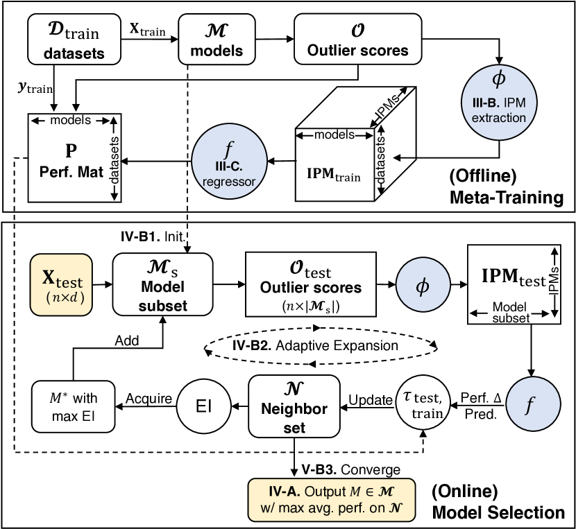
Figure 1: Main steps during the Offline and Online phases of ELECT.

II-B1 (Offline) Meta-training Overview

Given historical tasks $\mathbcal{D}_{\text{train}}$ and the new task $\mathcal{D}_{\text{test}}$ for model selection, the main idea is to first identify a subset of tasks $\mathcal{N}\subset\mathbcal{D}_{\text{train}}$ that are similar to $\mathcal{D}_{\text{test}}$, and then choose the model that performs the best on average on those “neighbor” tasks. Thus, a key ingredient of ELECT is an effective task similarity measure. Distinctly, it utilizes performance-driven task similarity: two tasks are similar if the performance rank-ordering of all the models on each task is similar.

Of course, the similarity of $\mathcal{D}_{\text{test}}$ to meta-train datasets cannot be computed based on the ground-truth model performances on $\mathcal{D}_{\text{test}}$ given that labels are unavailable for the input task (obviously, that would void the model selection problem altogether). A core idea of ELECT is to learn to estimate true performance from internal performance measures (IPMs) during meta-training. IPMs are unsupervised signals that are solely based on the input points and/or a given model’s output (e.g. outlier scores) that can be used to compare two models [23, 24]. However, they are noisy/weak indicators of performance [25]. ELECT makes the best use of these weak signals by learning to regress the IPMs of two models onto their true performance difference.

II-B2 (Online) Model Selection Overview

In the (online) model selection phase, given $\mathcal{D}_{\text{test}}$, we can build/run each candidate model on $\mathbf{X}_{\text{test}}$, extract the corresponding IPMs, and use the regressor (from meta-training) to estimate pairwise model performance differences for quantifying $\mathcal{D}_{\text{test}}$’s similarity to each meta-train dataset based on the all-pairs rank similarity of the models. However, building and internally evaluating all of the candidate models would be computationally expensive.

To avoid training all the models at test time, a core idea behind ELECT is to quantify similarity between $\mathcal{D}_{\text{test}}$ and meta-train tasks based on only a small subset of the models, which is carefully and adaptively picked and expanded. At each iteration, this strategy picks the next model to train on $\mathcal{D}_{\text{test}}$ with the best explore-exploit trade-off, where exploration (picking a model with high uncertainty in performance estimate) helps refine similarity and thereby update the set of neighbor tasks, and exploitation (picking a model with high-performance estimate) ensures that the neighbor tasks share similarity w.r.t. the well-performing models. Ultimately, the goal is to effectively identify similar historical tasks based on as few models run on $\mathcal{D}_{\text{test}}$ as possible. Upon convergence, the model with the largest average performance on the neighbor tasks (from the latest iteration) is reported as the selected model for $\mathcal{D}_{\text{test}}$.

We present the technical details of ELECT’s (offline) meta-training and (online) model selection phases in §III and §IV. Additional implementation details are given in Appx. A-A & A-B.

III ELECT: Meta-training (Offline)

The main component of meta-training is to learn, using historical (meta-train) tasks, how to quantify performance-based task similarity from imperfect indicators of performance, namely internal performance measures (IPMs). In the following, we introduce our task similarity measure (§III-A), specific IPMs used by ELECT (§III-B), and how to do the mapping between the two (§III-C).

III-A Performance-driven Task Similarity

Meta-learning carries the prior experience on historical tasks over to a new task, provided that the latter resembles some of the historical tasks. Thus, quantifying task similarity is crucial to the effectiveness of a meta-learning based approach [26].

Our work is most similar to the recent work by Zhao et al. [14] that developed the first unsupervised approach to outlier model selection. Their proposed MetaOD quantifies task similarity based on meta-features, which reflect general statistical properties of a dataset where the majority of the points are inliers. As such, two datasets with similar inlier distribution but different types of outliers may look similar w.r.t. meta-features, while different outlier models may be more effective in detecting different outlier types that they exhibit. In such scenarios, meta-feature similarity would be a poor indicator of model performance similarity.

In contrast to MetaOD, we propose a performance-driven similarity measure, where two tasks are deemed more similar, the more the same set of models perform well/poorly on both tasks. Arguably, ours is a direct means to the end goal—only when task similarity is defined in this performance-based fashion would it be natural (and even gold standard) to choose a model for a new task that performs well on its neighbor tasks.

Our performance-driven similarity is a rank-based measure, called the weighted Kendall’s tau rank correlation coefficient [27] ($\tau$ for short), which quantifies the similarity between the ordering of the candidate models by performance. Formally, let $\mathbf{P}_{i}\in\mathbb{R}^{m}$ depict the $i$-th row of $\mathbf{P}$ containing the detection performances of models $\mathcal{M}=\{M_{1},\ldots,M_{m}\}$ on dataset $\mathcal{D}_{i}$, and let $\Delta_{j,j^{\prime}}^{(i)}=\mathbf{P}_{i,j}-\mathbf{P}_{i,j^{\prime}}$ denote the difference between the performances of $M_{j}$ and $M_{j^{\prime}}$ on $\mathcal{D}_{i}$. Then, $\tau$ between two tasks $\mathcal{D}_{i}$ and $\mathcal{D}_{i^{\prime}}$ is defined as follows.

$$\tau^{(i,i^{\prime})}=\tau(\mathbf{P}_{i},\mathbf{P}_{i^{\prime}})=\frac{\sum_{j=1}^{m-1}\sum^{m}_{j^{\prime}=j+1}w_{j,j^{\prime}}^{(i,i^{\prime})}}{\sum_{j=1}^{m-1}\sum^{m}_{j^{\prime}=j+1}|w_{j,j^{\prime}}^{(i,i^{\prime})}|}\;,\quad\text{where}$$

$$w_{j,j^{\prime}}^{(i,i^{\prime})}=\begin{cases}1&\text{if }\Delta_{j,j^{\prime}}^{(i)}=\Delta_{j,j^{\prime}}^{(i^{\prime})}=0\\ \Delta_{j,j^{\prime}}^{(i)}\Big{/}\Delta_{j,j^{\prime}}^{(i^{\prime})}&\text{else if }|\Delta_{j,j^{\prime}}^{(i)}|\leq|\Delta_{j,j^{\prime}}^{(i^{\prime})}|\\ \Delta_{j,j^{\prime}}^{(i^{\prime})}\Big{/}\Delta_{j,j^{\prime}}^{(i)}&\text{else; i.e. }|\Delta_{j,j^{\prime}}^{(i)}|>|\Delta_{j,j^{\prime}}^{(i^{\prime})}|\\ \end{cases}$$ (1)

Intuitively, $\tau$ quantifies the concordance/discordance between pairwise model performances, where $\tau$ becomes smaller both when the rank-orders are discordant (i.e., $w_{j,j^{\prime}}$ is negative) and when they are concordant but the $\Delta$-differences are disproportionate (i.e., $w_{j,j^{\prime}}$ is near-zero). Put differently, two tasks are more similar when the models are ranked similarly, and also the perf. of each model are similar in value on both.

III-B Internal Performance Measures (IPMs)

To compute the similarity of a new task to historical meta-train tasks, we would need pairwise model performance differences on the new task. These model performances, of course, cannot be computed due to the lack of ground-truth labels. In fact, having these at hand would obviate the model selection problem altogether. Then, how can we really compute performance-driven task similarity?

The key idea is to learn a predictive model of ground-truth performance (which is available for meta-train tasks) from unsupervised indicators/features. The challenge is to identify such features that correlate with model performance. Notably, there exists a small literature on internal evaluation of outlier detection models [23, 24], and recently also unsupervised model selection strategies for deep representation learning based on other internal measures [28, 29]. These are called internal performance measures (IPMs) as they solely rely on the input samples, the outlier scores and/or the consensus between the candidate models. For example, consensus-based IPMs in principle associate closeness to an overall consensus of outlier scores/ranking with being a better model. We refer to §VI for more details on specific IPMs.

An IPM is exactly designed to compare models without any ground truth labels. Then, the question is why do not we simply and directly use an IPM for model selection? The reasons are two-fold. First, effectiveness-wise, IPMs are weak/noisy signals of true performance. As a recent study showed, they enable only slightly better model selection than random [25]. Distinctly, ELECT plugs the IPMs into a meta-learning framework, taking advantage of machine learning’s ability to map weak signals onto desired ones. Related, it would not be clear which IPM we should use for model selection (a “chicken-egg” scenario), provided several options. Notably, ELECT leverages all/any available IPMs as internal features in meta-training. Second, computation-wise, we would need to train each and every candidate model on $\mathcal{D}_{\text{test}}$ to obtain its IPM and compare it to others, leading to inhibitively high cost. In contrast, ELECT employs meta-learning to identify similar historical tasks based on a small subset of trained models on $\mathcal{D}_{\text{test}}$ while still being able to select among all of the candidate models via their (ground-truth) performance on these neighbor tasks.

III-C From IPMs to (True) Model Performance

At the core of ELECT’s meta-training is learning to map IPMs onto ground-truth performance by the supervision from the meta-train database. In particular, ELECT learns a regressor that maps the IPMs from two models onto their performance difference.

More formally, let $\phi(\cdot)$ denote the process of extracting various IPMs of model $M_{j}$ when trained on $\mathcal{D}_{i}$, and $\mathbf{m}_{i,j}$ denote the corresponding vector of IPMs. ELECT uses three IPMs; namely ModelCentrality (MC), HITS, and SELECT, as described in [25]. The regression function, named pairwise performance predictor, maps the IPMs of any pair of models $M_{j}$ and $M_{j^{\prime}}$ onto their performance difference on a dataset, i.e. $f(\mathbf{m}_{i,j},\mathbf{m}_{i,j^{\prime}})\mapsto\Delta_{j,j^{\prime}}^{(i)}$. In implementation we use LightGBM [30], while it is flexible in choosing any other. We design $f(\cdot)$ for pairwise prediction such that its output can be directly plugged into Eq. (1) for computing task similarity. We find it important to remark that provided with $\phi(\cdot)$ and the trained $f(\cdot)$ at test time, measuring performance-driven task similarity via $\tau$ becomes possible without using any ground-truth labels.

For clarity of presentation, we defer a few implementation details to Appx. §A-A, where we describe how to incrementally compute the IPMs as additional models are trained on the new input task at test time, as well as how to effectively train the regressor and use its predictions at test time.

IV ELECT: Model Selection (Online)

After the meta-training phase, ELECT is ready to admit a new task for model selection. Simply, it selects the highest performance model on meta-train tasks (or meta-tasks) that are very similar to the new task (§IV-A). It identifies these similar meta-tasks iteratively by refining the similarity estimates adaptively (§IV-B).

IV-A Model Selection via Similar Meta-tasks

Given a new task $\mathcal{D}_{\text{test}}$, we aim to identify its similar meta-train tasks (referred as the neighbor set $\mathcal{N}\subset\mathbcal{D}_{\text{train}}$). By the principle of meta-learning, the model(s) that outperform on the neighbor set is likely to outperform on the new task as well. Consequently, we could output the model with the largest average performance on the neighbor set as the selected model for the new task, that is,

$$\vspace{-0.05in}\operatorname*{arg\,max}_{M_{j}\in\mathcal{M}}\;\frac{1}{|\mathcal{N}|}\sum_{\mathcal{D}_{i}\in\mathcal{N}}\mathbf{P}_{i,j}\;.$$ (2)

If the model performances $\mathbf{P}_{\text{test}}$ were available for $\mathcal{D}_{\text{test}}$, we could iterate over the meta-train database to measure task similarity via Kendall’s tau in Eq. (1), and pick $\mathcal{N}$ to be the top $t$ most similar meta-train tasks, as shown in Eq. (3). Here $t$ denotes the size of the neighbor set (i.e. $|\mathcal{N}|=t$), which can be chosen by cross-validation on the meta-train database (see Appx. §A-B1 for details).

$$\mathcal{N}:=\underset{\scriptscriptstyle i=1\ldots n}{\text{top-}t}\;\tau^{(\text{test},i)}=\underset{\scriptscriptstyle i=1\ldots n}{\text{top-}t}\;\tau(\mathbf{P}_{\text{test}},\mathbf{P}_{i})$$ (3)

However, we cannot directly identify $\mathcal{N}$ due to the lack of ground-truth labels and thus evaluations $\mathbf{P}_{\text{test}}$ on the new task. Note the calculation of Kendall’s tau in Eq. (1) only depends on pairwise performance gaps (i.e. $\Delta$-differences) to measure concordance/discordance, where the trained regressor $f(\cdot)$ for pairwise performance gap prediction comes into play. By plugging the predicted pairwise gaps (i.e. $\widehat{\Delta}$-differences) of the new task into Eq. (1), we could therefore estimate its neighbor set $\mathcal{N}$ even when $\mathbf{P}_{\text{test}}$ is inaccessible.

Specifically, for the new task $\mathcal{D}_{\text{test}}$, we first get its outlier scores $\mathcal{O}_{\text{test}}=\mathcal{M}(\mathcal{D}_{\text{test}})$ and build the IPMs $\mathbf{m}_{\text{test}}=\phi(\mathcal{O}_{\text{test}})$ across candidate models.Note that We slightly abuse notation here and use $\mathbf{m}_{\text{test}}$ to depict the IPM vectors for all models, which is in fact a matrix. We could then predict the performance gap of any pair of models for $\mathcal{D}_{\text{test}}$ using the regressor $f(\cdot)$ by

$$\widehat{\Delta}_{j,j^{\prime}}^{(\text{test})}:=f(\mathbf{m}_{\text{test},j},\mathbf{m}_{\text{test},j^{\prime}})\approx\Delta_{j,j^{\prime}}^{(\text{test})}\;,$$ (4)

where $j=1\ldots m$ and $j<j^{\prime}$. The estimated Kendall-tau similarity ($\widehat{\tau}$) between the new task and meta-train tasks can be calculated using the predicted pairwise performance gaps on the new task $\widehat{\Delta}^{\text{test}}$ in Eq. (4) and the actual performance gaps on meta-train tasks $\Delta^{\text{train}}$, where e.g., we denote by $\widehat{\tau}^{\;(\text{test},i)}$ the estimated Kendall-tau similarity between $\mathcal{D}_{\text{test}}$ and the $i$-th meta-train dataset.

Then, by plugging the estimated task similarities into Eq. (3), we obtain the neighbor set $\mathcal{N}$ of the new task as the top-$t$ meta-train datasets with the highest estimated Kendall-tau similarity without relying on ground-truth labels, i.e.,

$$\mathcal{N}:=\underset{\scriptscriptstyle i=1...n}{\text{top-}t}\;\;\widehat{\tau}^{\;(\text{test},i)}\approx\underset{\scriptscriptstyle i=1...n}{\text{top-}t}\;\;\tau^{(\text{test},i)}\;.$$ (5)

IV-B Unsupervised Adaptive Search

IV-B1 Motivation and Initialization

Quantifying the task similarity by Kendall-tau using the full model set $\mathcal{M}=\{M_{1},\ldots,M_{m}\}$ (based on all ${m\choose 2}$ pairs of performance gaps) incurs high computational cost, as it involves model fitting to get outlier scores and extracting corresponding IPMs for all candidate models. We therefore propose to only measure task similarity based on a subset of the models, denoted $\mathcal{M}_{s}\subset\mathcal{M}$ for model subset. Initially, $\mathcal{M}_{s}$ can be set to a small random subset of $\mathcal{M}$, while a more careful initialization strategy may facilitate better similarity measurement. In ELECT, we design a coverage-maximization strategy for initializing $\mathcal{M}_{s}$, details of which are described in Appx. §A-B2. The ablation in §V-D1 shows it is significantly better than random initialization.

IV-B2 Iteration: Adaptively Expanding Model Subset

The initial $\mathcal{M}_{s}$ may not be sufficient to capture a complete picture of task similarity. Therefore, ELECT expands the model subset iteratively to refine the task similarity estimates and thereby obtain increasingly better estimates of the most similar datasets to $\mathcal{D}_{\text{test}}$.

Assume for now that an objective criterion exists for choosing the next model to be included in $\mathcal{M}_{s}$, then, the adaptive search proceeds as follows. In each iteration, we update the neighbor set $\mathcal{N}$ by the Kendall-tau similarities in Eq. (1) computed based on the model subset $\mathcal{M}_{s}$. Then, we quantify the value of each candidate model that is not already in $\mathcal{M}_{s}$ against the objective criterion and expand the model subset with the model $M^{*}$ having the maximum value, i.e. $\mathcal{M}_{s}:=\mathcal{M}_{s}\cup M^{*}$. In this way, we only need to fit on $\mathcal{D}_{\text{test}}$ (and get the corresponding IPMs) for the newly added model $M^{*}$ per iteration. To reduce the overall computational cost, the goal is to accurately identify highly similar neighbors $\mathcal{N}$ based on as few models trained on $\mathcal{D}_{\text{test}}$ as possible. It is important to note, however, that even if we train only a small subset of the models on the new task, upon identifying $\mathcal{N}$, we select a model from among all candidate models using Eq. (2).

What objective criterion is suitable for iteratively choosing the next model to be included in the model subset $\mathcal{M}_{s}$? We argue that the added model should meet two criteria, uncertainty and quality:

Criterion 1 (Uncertainty)

The performance (rank) of the added model should vary across the current neighbor set $\mathcal{N}$.

Criterion 2 (Quality)

The added model should outperform on the current neighbor set $\mathcal{N}$.

Notably, without uncertainty, $\mathcal{M}_{s}$ would end up choosing a group of similar models without enough representation of the full model space, which inhibits finding truly similar meta-tasks. A model with high performance variance over $\mathcal{N}$ indicates the datasets within the neighbor set exhibit disagreement (i.e. neighbors are not as similar among themselves), and including the model unlocks the opportunity to find truly similar meta-tasks. On the other hand, the quality criterion emphasizes that the added model should be a well-performing model on the neighbor set, as model selection mainly concerns “top models”. As such, we aim to identify the neighbor set based on task similarity regarding the well-performing models, whereas performance similarity based on underperforming models does not contribute much to the main goal of (top) model selection.

Now it is easy to see the trade-off between uncertainty and quality—the former emphasizes the model’s performance variation among the neighbor set while the latter expects high performance over all. This is akin to the explore-exploit trade-off; uncertainty drives exploration (for better neighbors) while quality drives exploitation (by promptly pinning a top model).

How can we quantify the uncertainty and quality of a candidate model (say, $M_{j}$)? Naturally, they can be respectively measured as the variance of the model’s performance, $\sigma^{2}_{j}=\sigma^{2}(M_{j}|\mathcal{N})$, and its average performance, $\mu_{j}=\mu(M_{j}|\mathcal{N})$, given the neighbor set. Thus, the simplest objective criterion that considers both uncertainty and quality criteria can be defined as the sum of the two:

$$\operatorname*{arg\,max}_{M_{j}\in\mathcal{M}\setminus\mathcal{M}_{s}}\;\;\underbracket{\sigma^{2}(M_{j}|\mathcal{N}))}_{\textrm{Uncertainty}}+\underbracket{\mu(M_{j}|\mathcal{N}))}_{\textrm{Quality}}$$ (6)

Can we define a better objective that automatically balances the trade-off between the two criteria? At this stage, we can recognize a connection to Sequential Model-based Bayesian Optimization (SMBO) [31]. As discussed in §VI, SMBO is a state-of-the-art paradigm for solving sequential problems like hyperparameter optimization in supervised settings [32]. As an iterative method, it relies on what-is-called an acquisition function $a(\cdot)$ that quantifies the utility of a candidate hyperparameter configuration (HPC) for the next evaluation [31]. In fact, as with the uncertainty/exploration and quality/exploitation trade-off, $a(\cdot)$ typically aims to balance between picking an HPC from the unexplored regions of the hyperparameter space and one with high estimated accuracy.

To capitalize on this connection, ELECT leverages the prominent acquisition function in SMBO called Expected (positive) Improvement (EI) [31] as our objective criterion to automatically balance the uncertainty-quality trade-off. In our setting, EI measures the expected improvement of including a candidate model into the model subset. The high EI value of a candidate model means that it has large performance variation and also high performance over the neighbor set $\mathcal{N}$. Moreover, one of the nice properties of EI is it has a closed-form expression under the Gaussian assumption, where the EI of a candidate model is defined as:

$$EI(M_{j}|\mathcal{N}):=\sigma_{j}\cdot[u_{j}\cdot\Phi(u_{j})+\varphi(u_{j})],\quad\text{where}\vspace{-0.1in}$$ (7)

$$u_{j}=\begin{cases}\frac{\mu_{j}-\mu_{s}^{*}}{\sigma_{j}}&\text{if }\sigma_{j}>0\;;\quad\textrm{and }\quad\bigg{\{}0\quad\text{if }\sigma_{j}=0\end{cases}\;.$$

In the above, $\Phi$ and $\varphi$ respectively denote the cumulative distribution and the probability density functions of standard Normal distribution, $\mu_{j}$ and $\sigma_{j}$ are the mean and the standard deviation of model $M_{j}$ across the neighbor set $\mathcal{N}$, and $\mu_{s}^{*}$ is the maximum value of the average model performance of $\mathcal{M}_{s}$ over $\mathcal{N}$, i.e.,

$$\mu_{s}^{*}=\underset{\scriptsize M_{h}\in\mathcal{M}_{S}}{\max}\;\;\frac{1}{|\mathcal{N}|}\sum_{\mathcal{D}_{i}\in\mathcal{N}}\mathbf{P}_{i,h}\;.$$

With the EI-based objective in Eq. (7), we include the highest EI candidate model to the model subset per iteration:

$$\mathcal{M}_{s}:=\mathcal{M}_{s}\cup\operatorname*{arg\,max}_{M_{j}\in\mathcal{M}\setminus\mathcal{M}_{s}}EI(M_{j}|\mathcal{N})\;.$$ (8)

To sum up, ELECT alternates between ($i$) updating the neighbor set $\mathcal{N}$ using Eq. (5) based on the (expanded) model subset $\mathcal{M}_{s}$, and ($ii$) expanding $\mathcal{M}_{s}$ using Eq. (8) based on the (updated) $\mathcal{N}$, until converged or termination criteria are met.

IV-B3 Convergence and Termination Criteria

ELECT can operate under two different practical settings: (1) hands-off: there is no time budget and (2) hands-on: the user has time constraints and the algorithm is to output a selected model whenever prompted.

Hands-off: When there is no time budget, ELECT stops when the neighbor set $\mathcal{N}$ stays unchanged in $p$ consecutive iterations, indicating that the identified similar meta-tasks have stabilized. We refer to parameter $p$ as “patience”, as a larger $p$ requires more iterations to converge. In the extreme case (when $p$ is set to a very large value), the algorithm would stop when all the models are added to the model subset, i.e. $\mathcal{M}_{s}=\mathcal{M}$. In this case, ELECT measures task similarity based on all models, falling back to the original setting (§IV-A) without the adaptive expansion. $p$ can be decided by cross-validation; see details in Appx. §A-B1.

Hands-on: When there is a time budget $b$ (iterations) to accommodate, ELECT stops the adaptive search when whichever one of two conditions occurs earlier: time budget is up, or patience criterion above is met. Note that the time budget need not be known to ELECT apriori, for it is an “any-time algorithm”: at any time the user prompts it during its course, it can always output a selected model as the one with the highest average performance on the neighbor set at the current iteration, based on Eq. (2).

IV-C Computational Complexity

Suppose that a task has $r$ samples and $d$ features on average, and the score computation of an OD model takes $C_{\text{train}}(r,d)$.

Lemma 1 (Meta-training)

The computational complexity of ELECT’s meta-training phase (offline) is $O(nmr+nm^{2})$.

Lemma 2 (Model selection)

The computational complexity of ELECT’s model selection phase (online) is $O[b(bn+mt+C_{\text{train}}(r,d))]$, for budget $b$ and neighbor count $t$.

See details in Appx. A-C. Note that the quadratic $m^{2}$ term in offline training is for measuring pairwise performance-driven task similarity, where $m$ is small (e.g., 297 in this study). In the online phase, the complexity is linear in both the number of meta-train datasets ($n$) and that of candidate models ($m$).

V Experiments

V-A Experiment Setting

Model Set. We configure 8 leading OD algorithms with various different settings of their associated hyperparameters to compose the model set $\mathcal{M}$ with 297 models (based on MetaOD [14]; the only diff. is we set n_neighbors of ABOD to $[3,5,10,15,20,25,50]$ for faster experimentation). We evaluate ELECT in two testbeds introduced below, with 39 and 30 datasets, respectively. For each testbed, we first generate the outlier scores of each model in $\mathcal{M}$ on each dataset, and then record the historical performance matrix $\mathbf{P}$. For models with built-in randomness, e.g., iForest and LODA with random feature splits, we run 5 random trials and record the average. All OD models are built using the PyOD library [33] on an Intel i7-9700 @3.00 GHz, 64GB RAM, 8-core workstation.

Testbeds. The key mechanism of meta-learning is to leverage the prior knowledge from truly similar tasks—where OD models perform similarly on both tasks. We create two testbeds with varying performance-driven task similarities (see Fig. 2).

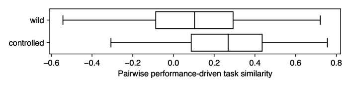
Figure 2: Pairwise performance-driven task similarity in the wild (med.=0.1035; lower similarity) and controlled (med.=0.2688; higher similarity) testbed.

(1) Wild testbed contains 39 independent datasets from 2 public OD repository (i.e., ODDS [34] and DAMI [4]) which simulates real-world use cases.

(2) Controlled testbed contains 30 datasets generated from 10 independent “mothersets” (from the Wild testbed), where 3 types of outliers (global, local, clustered) are injected into each motherset. As such, higher performance-driven task similarities are expected in the datasets with the same type of injected outliers (but from different mothersets), while their meta-feature similarities are low due to the independence of the mothersets. This testbed helps understand (i) if meta-feature methods can work when meta-feature similarity disagree with performance-driven similarity and (ii) to what extent the level of task similarity affects the performance of ELECT.

Baselines. We include 13 baselines for comparison. As shown in Table I, they can be categorized by (i) whether it selects a model; (ii) whether it is based on meta-learning; and (iii) whether it relies on meta-features. We use all 13 baselines in the wild testbed, and the 5 meta-feature-based methods in the controlled testbed as it is built to contrast performance- vs. meta-feature-based task similarities.

TABLE I: 13 baselines for comparison with categorization by (first row) whether it is a model selection method (second row) whether it uses meta-learning and (third row) whether it relies on meta-features (last row).

Category

iForest

LOF

ME

MC

SELECT

HITS

GB

ISAC

AS

ALORS

MetaOD

SS

IPM_SS

model selection

$\bullet$

$\bullet$

$\bullet$

$\bullet$

$\bullet$

$\bullet$

$\bullet$

$\bullet$

$\bullet$

$\bullet$

meta-learning

$\bullet$

$\bullet$

$\bullet$

$\bullet$

$\bullet$

$\bullet$

$\bullet$

meta-features

$\bullet$

$\bullet$

$\bullet$

$\bullet$

$\bullet$

Briefly, the baselines are organized as: (i) no model selection: directly/always use the same popular model (1) iForest [35] or (2) LOF [13], or the ensemble of all models (3) Mega Ensemble (ME); (ii) direct use of IPMs for model selection: (4) MC [25], (5) SELECT [25], and (6) HITS [25]; and (iii) meta-learning based methods: (7) Global Best (GB) selects the best performing model on meta-train database on average, (8) ISAC  [36], (9) ARGOSMART (AS)  [37], (10) ALORS [38], (11) MetaOD  [14] is the SOTA method, (12) Supervised Surrogates (SS) [39] directly regresses meta-features to performance $\mathbf{P}$, and (13) IPM-based Supervised Surrogates (IPM_SS) is a variant of SS but uses IPMs other than meta-features. Baselines (8)-(12) use meta-features.

Evaluation. In both testbeds, we use leave-one-out cross-validation (LOOCV) to split the meta-train/test. Each time we use one dataset as the input task, and the remaining datasets as meta-train. Meanwhile, we use cross-validation to decide the size of the neighbor set $\mathcal{N}$ for each input task, and use a fixed time budget $b=50$ as the convergence criteria. We use the area under the precision-recall curve (Average Precision or AP) as the performance measure, while it can be substituted with any other measures, e.g., the area under the receiver operating characteristic curve (ROC). Since the raw performance like AP is not comparable across datasets with varying magnitude, we report the AP-rank of a selected model, ranging from 1 (the best) to 297 (the worst)—thus smaller the better. To compare two methods, we use the paired Wilcoxon signed rank test across all datasets in the testbed (significance level $p<0.05$).

V-B Experiment Results

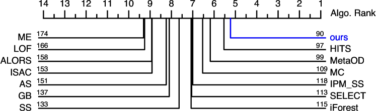
Figure 3: Comparison of avg. rank (lower is better) of algorithms w.r.t. performance across datasets in the wild testbed. ELECT outperforms all w/ the lowest avg. rank. Numbers on each line are the avg. AP-rank (lower is better) of the employed model (selected or otherwise) by each method.

V-B1 Results on Wild Testbed

As shown in Fig. 3, ELECT outperforms all baseline algorithms with the lowest avg. rank “in the wild”. Furthermore, Table II (left) shows that ELECT is the only algorithm that is not significantly different from the 55-$th$ best model. In other words, ELECT can consistently choose the top 18.5% model from a large pool of 297 models. Moreover, ELECT is significantly better than the no model selection baselines, LOF, iForest, ME, and other meta-learning baselines including GB, ISAC, ALORS, SS, and IPM_SS. For other baselines, p-value remains low although not significant at 0.05.

TABLE II: Pairwise statistical tests between ELECT and baselines by Wilcoxon signed rank test (statistically better method at $p$$<$$0.05$ in bold, both in bold if no difference). In wild testbed (left), ELECT is the only approach with no difference from the 55-$th$ best model. In controlled testbed (right), compared with meta-feature based baselines, ELECT is the only method with no difference from the 32-$th$ best model, and statistically better than all baselines.

Ours Baseline p-value ELECT 55-th Best 0.0541 ELECT iForest 0.0008 ELECT LOF 0.0004 ELECT ME 0.0188 ELECT MC 0.137 ELECT SELECT 0.0484 ELECT HITS 0.2142 ELECT GB 0 ELECT ISAC 0 ELECT AS 0.0147 ELECT ALORS 0.0002 ELECT MetaOD 0.2766 ELECT SS 0.0128 ELECT IPM_SS 0.0019

Ours Baseline p-value ELECT 32-th Best 0.0631 ELECT iForest N/A ELECT LOF N/A ELECT ME N/A ELECT MC N/A ELECT SELECT N/A ELECT HITS N/A ELECT GB N/A ELECT ISAC 0.0012 ELECT AS 0.003 ELECT ALORS 0.0001 ELECT MetaOD 0.0016 ELECT SS 0.0007 ELECT IPM_SS N/A

ELECT achieves the best performance with small ($<$$1$ min.) overhead. Fig. 4 shows the running time of the methods versus the avg. AP-rank of the employed model. Based on the avg. selection time per dataset, the methods can be categorized as i) super-fast methods that take less than 1 sec. (red zone); ii) fast methods that take less than 1 min. (blue zone); and iii) slow methods that use up to 10 min.s (green zone). Super-fast methods either directly employ a model (iForest, LOF) or simply report the historical best model (GB) with limited performance, showing the necessity for more effective meta-learning. In time-critical applications, employing iForest is a reasonable choice and it is indeed on the Pareto frontier of the time-performance trade-off. In the fast group, both MetaOD and ELECT are also on the Pareto frontier, showing the premise of effective meta-learning and the additional benefit of ELECT. Specifically, ELECT (avg. AP-rank$=$$90$) brings 10% performance improvement over MetaOD (avg. AP-rank$=$$99$), while being fast (avg. time$=$$47.10$s). For the slow group, in contrast, the higher runtime for model and IPM building does not yield improved performance over the fast methods.

IPMs do carry useful signals, and ELECT can leverage them more effectively. In fact, IPM-based MC, SELECT, and HITS rank high among all methods (Fig. 3), showing their potential in model selection. However, using IPMs directly for model selection incurs a large overhead in building all OD models and IPMs themselves at selection time, and therefore all of them fall in the slow group as shown in Fig. 4. Building on top of IPMs, ELECT shows superior results by “juicing out” useful information from IPMs via meta-learning, as well as reducing the runtime via sequential learning to prevent excessive model building.

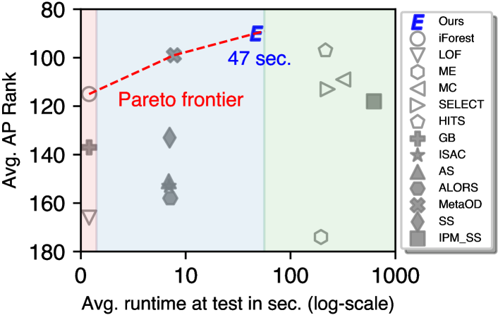
Figure 4: Avg. running time (log-scale) vs. avg. model AP-rank. Meta-learning methods depicted w/ solid markers. Based on runtime, methods are categorized as i) super-fast (in  ), ii) fast (in  ), and iii) slow (in  ). Pareto frontier (red dashed line) shows the best method under different time budgets. ELECT outperforms all with small time consumption (on avg. below 1 min. per task).

V-B2 Results on Controlled Testbed

Setup details. Meta-learning facilitates model selection for a new task by leveraging the prior knowledge from its truly similar meta-train tasks—where OD models perform similarly. The controlled testbed is built to create the scenario where there exist meta-train tasks with high performance-driven similarity but low meta-feature similarity, and vice versa. As meta-feature methods assume a high correlation between meta-feature similarity and task-performance similarity, they are likely to do poorly (i.e. select poor models) in this testbed as the assumption is violated.

To create such a setting, we randomly select 10 independent “mothersets” from the wild testbed, and inject one of 3 types of synthetic outliers (global, local, and clustered) by following [40], resulting in 30 datasets. Intuitively, different OD models are good at successfully detecting different types of outliers, irrespective of the underlying motherset. Therefore, we expect the datasets from different mothersets but with the same type of injected outliers to have high performance-driven task similarity yet low meta-feature similarity, while the datasets from the same mothersets but with different types of injected outliers to be vice versa.

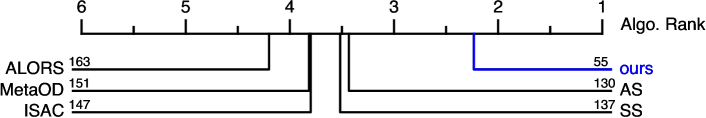
Figure 5: Comparison of avg. rank (lower is better) of algorithms w.r.t. performance across datasets in the controlled. ELECT outperforms all baselines.

Results. As shown in Fig. 5, ELECT is superior to all meta-feature-based baselines. Note that its avg. AP-rank is 55, while the avg. AP-rank of meta-feature baselines are all above 130. All these differences are significant at $p<0.005$ as shown in Table II (right). These results together show that the performance of meta-feature baselines suffers when performance-driven similarity is not correlated with meta-feature similarity. Distinctly, ELECT does not rely on meta-features and instead directly focuses on performance-driven similarity, leading to superior selection results.

As a meta-learning method, ELECT achieves better results with higher task similarity to meta-train. As shown in Fig. 2, the controlled testbed has higher task similarity than the wild. In Table II (right) ELECT is the only method that shows no statistical difference from the 32-$th$ best model, suggesting it can choose the top 11% model from $\mathcal{M}$, an improvement from the top 18.5% in the wild testbed. The selected models’ avg. AP-rank reflects the same—55 vs. 90 in the controlled and wild testbed, respectively.

V-C Case Study

It is interesting to trace how ELECT works over iterations on a given dataset, as shown in Table III for the Waveform dataset from the wild testbed. First we track the changes in the neighbor set: col. 2 reports the avg. similarity between Waveform and the identified neighbor set $\mathcal{N}$, and col. 3 shows the number of ground-truth top 5 most similar meta-train tasks in $\mathcal{N}$. ELECT gradually identifies both more similar and more of the top 5 meta-train tasks. From 1-$st$ to the 50-$th$ iteration, the avg. task similarity improves from 0.2276 to 0.3504., and the number of identified top 5 neighbors increases from 1 to 4. Note that out of the 38 meta-train tasks, only 7 of them have higher similarity than 0.3504. By identifying more and more similar meta-train tasks, ELECT gradually converges to kNN models as given in col. 4, which is indeed the best algorithm family for Waveform. Moreover, col. 5 shows that ELECT successfully identifies better models—the selected model’s AP-rank decreases from 77 to 38.

TABLE III: Trace of ELECT on Waveform dataset. Over iterations (col. 1), ELECT gradually identifies more similar meta-train tasks with increasing avg. similarity to Waveform (col. 2), more ground-truth top 5 neighbors (col. 3), and a better selected model with lower rank (col. 4). Best performing algorithm family on Waveform is kNN, which ELECT successfully identifies during its adaptive search.

Iter.	Avg. Sim.	# Matched neighbors	The selected model	The selected model rank
1	0.2776	1	(’LOF’, (’manhattan’, 5))	77
2	0.2876	1	(’COF’, 10)	70
$\ldots$	$\ldots$	$\ldots$	$\ldots$	$\ldots$
11	0.3304	2	(’LOF’, (’manhattan’, 10))	76
12	0.3493	3	(’LOF’, (’euclidean’, 20))	71.5
$\ldots$	$\ldots$	$\ldots$	$\ldots$	$\ldots$
21	0.4351	4	(’kNN’, (’mean’, 5))	50
22	0.4351	4	(’kNN’, (’mean’, 5))	50
$\ldots$	$\ldots$	$\ldots$	$\ldots$	$\ldots$
31	0.2960	4	(’kNN’, (’mean’, 15))	38
32	0.4351	4	(’kNN’, (’mean’, 5))	50
$\ldots$	$\ldots$	$\ldots$	$\ldots$	$\ldots$
49	0.3504	4	(’kNN’, (’mean’, 15))	38
50	0.3504	4	(’kNN’, (’mean’, 15))	38

V-D Ablation Studies and Other Analysis

V-D1 Model initialization

ELECT uses proposed coverage-driven initialization of the model subset $\mathcal{M}_{s}$ (see Appx. §A-B2). Fig. 6 shows that its AP-rank (median=87.5) is notably lower than that of random initialization (median=133). The difference, by one-sided Wilcoxon signed rank test, is statistically significant at $p=0.0204$.

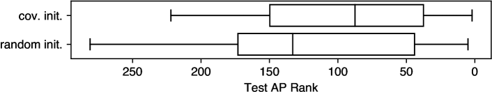
Figure 6: Ablation of coverage init. (med.=87.5) vs. random init. (med.=133).

V-D2 The Effect of Model Inclusion Criteria

Fig. 7 shows the performance comparison between using EI (balancing both exploitation and exploration) in Eq. (7) and the greedy objective (exploitation only) that adds the model with the highest performance on $\mathcal{N}$ during adaptive search (see §IV-B2). One-sided Wilcoxon signed rank test shows that the former (median=87.5) is statistically better (at $p=0.0203$) than the latter (median=105), justifying the use of EI.

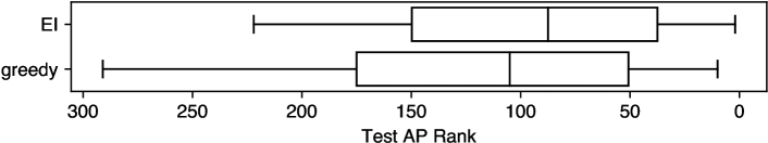
Figure 7: Ablation of using EI (med.=87.5) vs. greedy without exploration (med.=105) during the adaptive search.

VI Related Work

Model Selection for Outlier Detection. There is no shortage of unsupervised OD algorithms in the literature, while most are sensitive to their hyperparameter (HP) choices [4]. Stunningly, outlier model selection (OMS) is understudied [5].

We can categorize the (short list of) approaches to OMS into two. The first group focuses on using internal evaluation/performance measures based solely on model output and/or input data [23, 24]. As a recent study showed [25], those are noisy performance indicators that are only slightly better than random selection. The second category consists of learning-based approaches. A subset of these are semi-supervised [19, 20], which use clean/inlier-only data for training, and a small validation set with labels for model selection—inapplicable to the U(nsupervised)OMS problem. The only existing work on UOMS is the meta-learning based MetaOD [14]. Distinctly, we eliminate the hand-crafted meta-features and instead employ performance-driven similarity between tasks. Consequently, our ELECT outperforms MetaOD [14] on two separate testbeds.

Hyperparameter Opt. (HPO) and Meta-Learning.  HPO has gained significant attention within AutoML owing to the advent of complex models with large HP spaces that are costly to train and thereby to tune [21]. Besides model-free techniques such as grid or random search [15], Bayesian optimization and the adaptation of Sequential Model-Based Optimization (SMBO) [31] is one of the main lines of work in HPO. The idea is to iterate between (i) fitting a surrogate performance function onto past HP evaluations, and (ii) using it to choose the next HP based on an acquisition function. Well-established SMBO approaches include SMAC [16] and Auto-WEKA [17]. We remark that SMBO cannot directly be used for UOMS, as we cannot evaluate model performance reliably to train an effective surrogate. Instead, ELECT employs meta-learning to estimate the mean and variance of a candidate model’s performance (to be used for acquisition) based on similar historical tasks.

Meta-learning has been used for HPO in various forms [41]; e.g. to warm-start SMBO [42], prune the HP search space [43], and transfer surrogate models [44]. Active testing [45] has used meta-learning for model selection, which differs from our work in two key aspects. First, their acquisition is fully exploitative and does not factor in variance. More importantly, it is supervised: computes task similarity based on model performance evaluated on ground-truth.

VII Conclusion

In the face of numerous outlier detection algorithms with various hyperparameters, there exists a shortage of principled approaches to unsupervised outlier model selection—a vastly understudied subject. Toward filling this gap in the literature, we proposed ELECT, a meta-learning approach that selects a candidate model for a new task based on its performance-based similarity to historical (meta-train) tasks. ELECT adaptively identifies these neighbor tasks, as such, it can flexibly output a selected model in an any-time fashion, accommodating varying time budgets. Through extensive experiments, we showed that ELECT significantly outperforms a wide range of prior as well as more recent baselines. Future work includes extending to UOMS for deep learning based outlier models.

Appendix A Implementation Details

A-A (Offline) Meta-training Details for §III

A-A1 Building Internal Performance Measures (IPMs)

As described in §III-B and III-C, IPMs are used as the input features of the performance predictor $f(\cdot)$. In ELECT, we use three consensus-based IPMs (i.e., MC, SELECT, and HITS) as they are reported to carry useful signals in model selection [25]. Namely, consensus-based IPMs consider the resemblance to the overall consensus of outlier scores as a sign of a better model; their computation requires a group of models.

In [25], Ma et al. use all models in $\mathcal{M}$ for building IPMs, leading to high cost in generating outlier scores and then IPMs. To reduce the cost, we identify a small subset of representative models $\mathcal{M}_{A}\in\mathcal{M}$ called the anchor set (i.e., $|\mathcal{M}_{A}|\ll|\mathcal{M}|$), for calculating IPMs. That is, we generate the IPMs of a model with regard to its consensus to $\mathcal{M}_{A}$ rather than $\mathcal{M}$. Similar to forward feature selection [46], the anchor set can be identified in a forward fashion (i.e., iteratively expanding the set) and cross-validation on the meta-train database.

A-A2 Pairwise Performance Predictor

As shown in §III-C, the predictor $f(\cdot)$ maps the vector of IPMs of a pair of models to their performance difference. To that end, we train a LightGBM regressor [30] by enumerating all ${m\choose 2}$ model pairs for each task in meta-train database, where the hyperparameters are set by cross-validation.

A-B (Online) Model Selection Details for §IV

A-B1 Hyperparameters

The hyperparameters are chosen by LOOCV on the meta-train set. To that end, we find the following settings works well in both testbeds: (i) the size of the neighbor set, $|\mathcal{N}|=t$, equals to 5 (§IV-A) (ii) the initial size of the model subset, $|\mathcal{M}_{s}|$, equals to 7 (§IV-B1) and (iii) patience $p$ equals to 17 (§IV-B3).

A-B2 Model Subset Initialization

Other than random sampling, we design a coverage-driven strategy for initializing $\mathcal{M}_{s}$ in §IV-B1. Intuitively, we expect $\mathcal{M}_{s}$ provides differentiability among datasets—the models’ performance in $\mathcal{M}_{s}$ on different datasets should vary. To this end, the coverage-driven strategy iteratively builds the initial $\mathcal{M}_{s}$ by including the model that performs best (a top model) or worst (a bottom model) on the most meta-train tasks that have not been “covered”. A task is said “covered” if both its top and bottom models (at least one) are already included in the model subset.

A-C Detailed Complexity Analysis

Suppose each task has $r$ samples and $d$ features on average, and the score computation of an OD model takes $C_{\text{train}}(r,d)$.

Meta-training involves (i) IPM generation (§III-B) for $n$ meta-train tasks on all $m$ models; MC, SELECT, and HITS have $O(nr)$, $O(nmr)$, $O(nmr)$, respectively; (ii) training of pairwise performance predictor (i.e., lightGBM, §III-C) uses the input data composed by $n$ tasks, each with ${m\choose 2}$ model pairs by enumeration, leading to $O(nm^{2})$ complexity; and (iii) building the anchor set with forward selection (§A-A1) takes $O(nmr)$. Overall runtime is $O(nmr+nm^{2})$.

Model selection first initializes the model subset $\mathcal{M}_{s}$ with the coverage-driven strategy (§IV-B1), yielding $O(nm)$. For each initial model in $\mathcal{M}_{s}$, outlier score and IPM generation take $O(C_{\text{train}}(r,d)+r)$. In each of $b$ iterations of adaptive search (§IV-B2), ELECT (i) predicts the model performance with $O(bn)$ complexity (ii) identifies the next model to be included in $\mathcal{M}_{s}$ with EI, taking $O(mt)$ and (iii) gets the next model’s outlier scores and IPMs with $O(C_{\text{train}}(r,d)+r)$ runtime. The total selection runtime is $O[b(bn+mt+C_{\text{train}(r,d)})]$.

References

- [1] C. C. Aggarwal, Outlier Analysis. Springer, 2013.
- [2] G. Pang, C. Shen, L. Cao, and A. V. D. Hengel, “Deep learning for anomaly detection: A review,” CSUR, vol. 54, no. 2, pp. 1–38, 2021.
- [3] S. Raschka, “Model evaluation, model selection, and algorithm selection in machine learning,” arXiv preprint arXiv:1811.12808, 2018.
- [4] G. O. Campos, A. Zimek, J. Sander, R. J. G. B. Campello, B. Micenková, E. Schubert, I. Assent, and M. E. Houle, “On the evaluation of unsupervised outlier detection,” DAMI, vol. 30, no. 4, pp. 891–927, 2016.
- [5] M. Bahri, F. Salutari, A. Putina, and M. Sozio, “Automl: state of the art with a focus on anomaly detection, challenges, and research directions,” Int J Data Sci Anal, 2022.
- [6] D. H. Wolpert and W. G. Macready, “No free lunch theorems for optimization,” IEEE Trans. Evol. Comput., vol. 1, pp. 67–82, 1997.
- [7] S. Han, X. Hu, H. Huang, M. Jiang, and Y. Zhao, “ADBench: Anomaly detection benchmark,” in NeurIPS, 2022.
- [8] P. Marteau, S. Soheily-Khah, and N. Béchet, “Hybrid isolation forest - application to intrusion detection,” CoRR, vol. abs/1705.03800, 2017.
- [9] A. Lazarevic, L. Ertöz, V. Kumar, A. Ozgur, and J. Srivastava, “A comparative study of anomaly detection schemes in network intrusion detection,” in SDM, 2003.
- [10] N. Kumar and U. Kumar, “Anomaly-based network intrusion detection: An outlier detection techniques,” in SoCPaR, vol. 614. Springer, 2016.
- [11] C. C. Aggarwal and S. Sathe, “Theoretical foundations and algorithms for outlier ensembles.” SIGKDD Explor., vol. 17, no. 1, pp. 24–47, 2015.
- [12] M. Goldstein and S. Uchida, “A comparative evaluation of unsupervised anomaly detection algorithms for multivariate data,” PLOS, 2016.
- [13] M. M. Breunig, H.-P. Kriegel, R. T. Ng, and J. Sander, “LOF: Identifying density-based local outliers.” in SIGMOD. ACM, 2000, pp. 93–104.
- [14] Y. Zhao, R. Rossi, and L. Akoglu, “Automatic unsupervised outlier model selection,” NeurIPS, vol. 34, 2021.
- [15] L. Li, K. Jamieson, G. DeSalvo, A. Rostamizadeh, and A. Talwalkar, “Hyperband: A novel bandit-based approach to hyperparameter optimization,” JMLR, vol. 18, no. 1, pp. 6765–6816, 2017.
- [16] F. Hutter, H. H. Hoos, and K. Leyton-Brown, “Sequential model-based optimization for general algorithm configuration,” in LION, 2011.
- [17] C. Thornton, F. Hutter, H. H. Hoos, and K. Leyton-Brown, “Auto-WEKA: Combined selection and hyperparameter optimization of classification algorithms,” in KDD, 2013, pp. 847–855.
- [18] X. He, K. Zhao, and X. Chu, “AutoML: A survey of the state-of-the-art,” Knowledge-Based Systems, vol. 212, p. 106622, 2021.
- [19] Y. Li, Z. Chen, D. Zha, K. Zhou, H. Jin, H. Chen, and X. Hu, “Autood: Neural architecture search for outlier detection,” in ICDE. IEEE, 2021.
- [20] Y. Li, D. Zha, P. Venugopal, N. Zou, and X. Hu, “PyODDS: An end-to-end outlier detection system with automated machine learning,” in Companion Proceedings of the WebConf, 2020, pp. 153–157.
- [21] M. Feurer and F. Hutter, “Hyperparameter optimization,” in Automated machine learning. Springer, Cham, 2019, pp. 3–33.
- [22] L. Yang and A. Shami, “On hyperparameter optimization of machine learning algorithms: Theory and practice,” Neurocomputing, 2020.
- [23] N. Goix, “How to evaluate the quality of unsupervised anomaly detection algorithms?” arXiv preprint arXiv:1607.01152, 2016.
- [24] H. O. Marques, R. J. Campello, J. Sander, and A. Zimek, “Internal evaluation of unsupervised outlier detection,” TKDD, vol. 14, 2020.
- [25] M. Q. Ma, Y. Zhao, X. Zhang, and L. Akoglu, “A large-scale study on unsupervised outlier model selection: Do internal strategies suffice?” CoRR, vol. abs/2104.01422, 2021.
- [26] J. Vanschoren, “Meta-learning: A survey,” arXiv preprint arXiv:1810.03548, 2018.
- [27] G. S. Shieh, “A weighted kendall’s tau statistic,” Statistics & Probability Letters, vol. 39, no. 1, pp. 17–24, Jul. 1998.
- [28] S. Duan, L. Matthey, A. Saraiva, N. Watters, C. Burgess, A. Lerchner, and I. Higgins, “Unsupervised model selection for variational disentangled representation learning.” in ICLR. OpenReview.net, 2020.
- [29] Z. Lin, K. Thekumparampil, G. Fanti, and S. Oh, “InfoGAN-CR and ModelCentrality: Self-supervised model training and selection for disentangling GANs,” in ICML, 2020, pp. 6127–6139.
- [30] G. Ke, Q. Meng, T. Finley, T. Wang, W. Chen, W. Ma, Q. Ye, and T.-Y. Liu, “Lightgbm: A highly efficient gradient boosting decision tree,” NIPS, vol. 30, pp. 3146–3154, 2017.
- [31] D. R. Jones, M. Schonlau, and W. J. Welch, “Efficient global optimization of expensive black-box functions,” J. Glob. Optim., vol. 13, 1998.
- [32] J. Snoek, H. Larochelle, and R. P. Adams, “Practical bayesian optimization of machine learning algorithms,” in NIPS, 2012, pp. 2960–2968.
- [33] Y. Zhao, Z. Nasrullah, and Z. Li, “Pyod: A python toolbox for scalable outlier detection,” JMLR, vol. 20, pp. 96:1–96:7, 2019.
- [34] S. Rayana, “ODDS library,” 2016.
- [35] F. T. Liu, K. M. Ting, and Z.-H. Zhou, “Isolation forest,” in ICDM, 2008.
- [36] S. Kadioglu, Y. Malitsky, M. Sellmann, and K. Tierney, “Isac - instance-specific algorithm configuration.” in ECAI, vol. 215, 2010, pp. 751–756.
- [37] M. Nikolic, F. Maric, and P. Janicic, “Simple algorithm portfolio for sat.” Artif. Intell. Rev., vol. 40, no. 4, pp. 457–465, 2013.
- [38] M. Misir and M. Sebag, “Alors: An algorithm recommender system.” Artif. Intell., vol. 244, pp. 291–314, 2017.
- [39] L. Xu, F. Hutter, J. Shen, H. H. Hoos, and K. Leyton-Brown, “Satzilla2012: Improved algorithm selection based on cost-sensitive classification models,” Proceedings of SAT Challenge, pp. 57–58, 2012.
- [40] G. Steinbuss and K. Böhm, “Benchmarking unsupervised outlier detection with realistic synthetic data,” TKDD, vol. 15, no. 4, 2021.
- [41] M. Wistuba, N. Schilling, and L. Schmidt-Thieme, “Hyperparameter optimization machines,” in DSAA. IEEE, 2016, pp. 41–50.
- [42] M. Feurer, J. Springenberg, and F. Hutter, “Initializing bayesian hyperparameter optimization via meta-learning,” in AAAI, vol. 29, 2015.
- [43] M. Wistuba, N. Schilling, and L. Schmidt-Thieme, “Hyperparameter search space pruning–a new component for sequential model-based hyperparameter optimization,” in PKDD. Springer, 2015, pp. 104–119.
- [44] D. Yogatama and G. Mann, “Efficient transfer learning method for automatic hyperparameter tuning,” in AISTATS, 2014, pp. 1077–1085.
- [45] R. Leite, P. Brazdil, and J. Vanschoren, “Selecting classification algorithms with active testing,” in MLDM. Springer, 2012, pp. 117–131.
- [46] I. Guyon and A. Elisseeff, “An introduction to variable and feature selection,” JMLR, vol. 3, no. Mar, pp. 1157–1182, 2003.