Extra-Newton: A First Approach to Noise-Adaptive Accelerated Second-Order Methods

Abstract.

This work proposes a universal and adaptive second-order method for minimizing second-order smooth, convex functions. Our algorithm achieves $O(\sigma/\sqrt{T})$ convergence when the oracle feedback is stochastic with variance $\sigma^{2}$, and improves its convergence to $O(1/T^{3})$ with deterministic oracles, where $T$ is the number of iterations. Our method also interpolates these rates without knowing the nature of the oracle apriori, which is enabled by a parameter-free adaptive step-size that is oblivious to the knowledge of smoothness modulus, variance bounds and the diameter of the constrained set. To our knowledge, this is the first universal algorithm with such global guarantees within the second-order optimization literature.

1. Introduction

Over the last few decades, first-order (convex) minimization methods have gained popularity for modern machine learning and optimization problems due to their efficient per-iteration cost and global convergence properties. The literature on first-order methods is rather dense and extensive with a concrete, thorough understanding of the optimal global convergence behavior. Focusing on the more relevant settings of smooth, convex minimization, the lower bounds have been well-established; $O(\sigma/\sqrt{T})$ when the gradient feedback is noisy with variance $\sigma^{2}$, and $O(1/T^{2})$ under deterministic first-order oracles [52, 58]. Under slight variations of the aforementioned problem setting, there exists an extensive amount of work that enjoys the latter, “accelerated” rate [56, 57, 53, 65, 69, 39, 2, 41, 67, 19, 18, 35, 31, 6, 44].

On the contrary to its first-order analogue, the literature on global convergence of second-order, smooth methods is notably sparse with many open questions standing even in the simplest problem formulations. Following the pioneering works of Bennett [11], Kantorovich [33], Newton’s method and its variations [40, 46] are considered as the staple of second-order methods in optimization. Although its powerful local convergence behavior has been repeatedly demonstrated [17, 38], studies on its global behavior are relatively limited. Prior attempts at tackling global convergence mostly make additional structural assumptions on the objective function [61, 47, 38] or assume extra regularity conditions on the Hessian [34] beyond the simplest smooth and convex setting. Over the last decade, we have witnessed important progress towards a more complete theory of globally-convergent second-order methods (more on this shortly), and yet there remains many important questions unanswered, which we will delve into in this paper.

To motivate the perspective in our technical endeavour, we take a small detour to introduce the idea of universality, which we particularly characterize as adaptation to the level of noise in oracle feedback. Enabled by the recent advances in online optimization, universal first-order algorithms essentially attain the $O(\sigma/\sqrt{T}+1/T^{2})$ convergence for convex minimization problems, interpolating between stochastic and deterministic rates. There exist a plethora of algorithms that enjoy this rate under different sets of assumptions for both minimization scenarios (for convex and non-convex settings, we refer the reader to [39, 35, 22, 31, 6] and [68, 42, 36, 45], respectively), and the more general framework of variational inequalities [8, 5, 66, 25, 3, 26, 4]. However, we observe that such universal results do not exist in second-order literature, hence, it is only natural to ask,

Can we design a simple second-order method that will achieve
accelerated universal rates beyond $O(\sigma/\sqrt{T}+1/T^{2})$?

More recently, global sub-linear convergence rates for second-order methods have been characterized by [59] for second-order smooth and convex setting. Essentially, the so-called Cubic Regularized Newton’s Method combines the quadratic Taylor approximation in the typical Newton update with a cubic regularization term. At the expense of solving a cubic problem, this method achieves $O(1/T^{2})$ convergence rate. Shortly after, Nesterov [55] proposes an accelerated version of the cubic regularization idea with $O(1/T^{3})$ value convergence, pioneering a new direction of research in the study of globally-convergent second-order methods [49]. This idea has been studied further for different settings in convex optimization [28, 29] with the same accelerated $O(1/T^{3})$ rate and extended to non-convex realm [14, 15], obtaining the analogous rates of $O(1/T^{2/3})$ and $O(1/T^{1/3})$ for finding first-order and second-order stationary points, respectively, leading the way for further investigations [10, 21, 16].

Notice that accelerated cubic regularization is sub-optimal such that recent studies prove a respective lower-bound for second-order smooth, convex problems as $O(1/T^{7/2})$ [1, 7]. The first line of research that shrinks the gap between the upper and lower bounds for achieving an almost-optimal (more on this shortly) convergence [60] is the so-called “bisection-type” methods. Pioneered by Monteiro and Svaiter [50], these class of algorithms propose a conceptual method where the step-size of the algorithm implicitly depends on the next iterate. To resolve, the authors propose a bisection procedure that simultaneously finds a step-size/next iterate pair that satisfies the conditions of the iterative update, which enables the convergence rate of $O(1/T^{7/2})$, modulo the complexity of bisection procedure. This idea was very recently generalized for higher-order tensor methods [23]. Not so surprisingly, the same construction finds application in variational inequality (VI) and min-max optimization literature [12, 30]. Very recently and concurrently to our work, [13] propose the first bisection free acceleration for second-order methods, that achieves the optimal $O(1/T^{7/2})$. The authors define an explicit, deterministic procedure called MS oracle and compute the step-size using a standard line-search procedure enabling them to achieve optimal rates while adaptively computing the step-size without needing to know the smoothness constant.

Although there are promising results with an increasing interest into second-order –and also higher-order– methods, we identify three main shortcomings in the literature, which we will systematically address in the sequel. First, bisection-type methods achieve the optimal convergence rate however, the search procedure is computationally very prohibitive [60, 43] and the resulting algorithms are complicated with many interconnected components. On the other hand, cubic regularization-based ideas propose a simple construction that achieves acceleration beyond $O(1/T^{2})$ however, similar to previous methods, they either require the knowledge of smoothness constant or need to execute a standard line-search procedure to estimate it locally. A common drawback for both approaches is that the algorithmic constructions are designed for handling only deterministic oracles and it is an open question whether such frameworks could immediately accommodate stochastic first and second-order information.

Our contributions:

To address the aforementioned issues, we developed the first universal and adaptive second-order algorithm, Extra-Newton, for convex minimization. We summarize our contributions as follows:

1. We prove Extra-Newton achieves the global convergence rate of $O(\frac{\sigma_{g}}{\sqrt{T}}+\frac{\sigma_{H}}{T^{3/2}}+\frac{LD^{3}}{T^{3}})$ that adapts simultaneously to the variance in the gradient oracle ($\sigma_{g}$) and Hessian oracle ($\sigma_{H}$) achieving the first universal convergence result in the literature.

2. Our method is completely oblivious to any problem-dependent parameters including smoothness modulus, variance bounds on stochastic oracles, diameter of the constraint set and any possible bounds on the gradient and Hessian.

3. We design the first adaptive step-size, in the sense of [20, 63], that successfully incorporates second-order information “on-the-fly”. While doing so, we bypass any bisection or linesearch procedure, and propose a simple, intuitive algorithmic framework.

From a technical point of view, what will allow us to achieve these results is the combination of three principal ingredients: (it ) proposing appropriate adjustments to Extra-Gradient [37] that was originally designed for solving variational inequalities and min/max problems; (it ) an “optimistic” weighted iterate averaging scheme accompanied by an appropriate gradient rescaling strategy in the spirit of [67, 19, 35] which allows us to obtain an accelerated rate of convergence by means of a generalized online-to-batch conversion (Theorem 3.3), and (it ) the glue that holds these elements together is an adaptive learning rate inspired by [63, 35, 4] which automatically rescales aggregated gradients and second order information. In what follows, we shall explicate these arguments.

Table 1. A survey on first and second-order algorithms with key properties

	AGD [56]	UniXGrad [35]	Reg. Newton [49]	Accel. Cubic Reg. [55]	ANPE [50]	OptMS [13]	Extra Newton [ours]
Rate	$\frac{1}{T^{2}}$	$\frac{\sigma_{g}}{\sqrt{T}}+\frac{1}{T^{2}}$	$\frac{1}{T^{2}}$	$\frac{1}{T^{3}}$	$\frac{1}{T^{7/2}}$	$\frac{1}{T^{7/2}}$	$\frac{\sigma_{g}}{\sqrt{T}}+\frac{\sigma_{H}}{T^{3/2}}+\frac{1}{T^{3}}$
Bisection	✗	✗	✗	✗	✓	✗	✗
Adapts to $L$	✗	✓	✗	Partial	✗	✓	✓
Noise-adaptive	✗	✓	✗	✗	✗	✗	✓

2. Problem setup

Throughout the sequel, we will be focusing on solving (constrained) convex minimization problems of the general form:

minimize $$\quad f(x)$$ (Opt)

subject to $$\quad x\in\mathcal{X}.$$

Formally, in the above $\mathcal{X}$ is a convex and compact subset of a $d$- dimensional normed space $\mathcal{V}\cong\mathbb{R}^{d}$ with diameter $D=\max_{x,y\in\mathcal{X}}\lVert{x-y}\rVert$, and $f:\mathcal{V}\to\mathbb{R}\cup\{+\infty\}$ is a proper, lower semi-continuous, convex function with $\text{dom}f=\{x\in\mathbb{R}^{d}:f(x)<+\infty\}\subset\mathcal{X}$. To that end, we make a set of blanket assumptions for (Opt). Following the vast literature of constrained convex minimization [54, 9], we consider “simple” constraint sets, i.e.,

Assumption 2.1.

The constraint set $\mathcal{X}$ of (Opt) possesses favorable geometry which facilitates a tractable projection operator.

In order to avoid trivialities, we also assume that the said problem admits at least a solution, i.e.

Assumption 2.2.

The solution set $\mathcal{X}^{\ast}=\operatorname*{arg\,min}_{x\in\mathcal{X}}f(x)$ of (Opt) is non-empty.

Furthermore, we assume that there exists a Lipschitz continuous selection $x\mapsto\nabla^{2}f(x)\in\mathbb{R}^{d\times d}$, i.e.,

$$\|\nabla^{2}f(x)-\nabla^{2}f(x^{\prime})\|\leq L\|x-x^{\prime}\|\;\;\forall x,x^{\prime}\in\mathcal{X}$$ (H-smooth)

and in addition it satisfies the second order approximation:

$$f(x)=f(x^{\prime})+\langle\nabla f(x^{\prime})\mathopen{},\mathopen{}x-x^{\prime}\rangle+\frac{1}{2}\langle{\nabla^{2}f(x^{\prime})(x-x^{\prime})},{x-x^{\prime}}\rangle+O\left({\lVert{x-x^{\prime}}\rVert^{3}}\right)$$ (Taylor)

To that end, combining (H-smooth) and (Taylor) we readily get the following inequality:

$$\lVert{\nabla f(x)-\nabla f(x^{\prime})-\nabla^{2}f(x^{\prime})(x-x^{\prime})}\rVert\leq\frac{L}{2}\lVert{x-x^{\prime}}\rVert^{2}$$ (1)

The above equivalences are well-established and hence we omit their proofs (we defer for a panoramic view to [70])

Oracle feedback structure

From an algorithmic point of view, we aim to solve (Opt) by using methods that require access to a (stochastic) first and second order-oracle. Before we move forward with the methodology, we shall introduce the definitions and notations for this oracle model which we will use in algorithm definitions and technical discussions. Let $g(x,\xi)$ denote the stochastic gradient evaluated at $x$ with randomness defined by $\xi$ and $H(x,\xi)$ be the stochastic Hessian at $x$ with $\xi$ describing the randomness of the oracle, such that

$$\mathbb{E}\left[\,g(x,\xi)\mid x\,\right] =\nabla f(x),\qquad\quad\,\,\mathbb{E}\left[\,\lVert{g(x,\xi)-\nabla f(x)}\rVert^{2}\mid x\,\right]\leq\sigma_{g}^{2}$$ (2)

$$\mathbb{E}\left[\,H(x,\xi)\mid x\,\right] =\nabla^{2}f(x),\qquad\mathbb{E}\left[\,\lVert{H(x,\xi)-\nabla^{2}f(x)}\rVert^{2}\mid x\,\right]\leq\sigma_{H}^{2}$$

Due to space constraints, we will also define an operator that accommodates second-order information and its respective stochastic counterpart.

$$\mathbf{F}(x;x^{\prime}) =\nabla f(x^{\prime})+\frac{1}{2}\nabla^{2}f(x^{\prime})(x-x^{\prime})$$ (3)

$$\mathbf{\tilde{F}}(x;x^{\prime},\xi) =g(x^{\prime},\xi)+\frac{1}{2}H(x^{\prime},\xi)(x-x^{\prime})\$$

where $\mathbf{F}$ is essentially the gradient (with respect to $x$) of the second-order Taylor polynomial. By definition, the operator $\mathbf{F}$ satisfies the second-order smoothness property in Eq. (1)

3. Method

In this section, we shall establish our universal second-order framework. Our presentation evolves around three key components: choosing the appropriate algorithmic template with the key motivations behind it, solving implementability issues that commonly arise in higher-order methods and finally designing a universal algorithm that can handle deterministic and noisy oracle feedback simultaneously without having prior knowledge. Our point of departure is the popular Extra-Gradient (EG) template; originally introduced by Korpelevich [37] and further developed in Nemirovski [51],

$$X_{t+\frac{1}{2}} =\Pi_{\mathcal{X}}\left({X_{t}-\gamma_{t}\nabla f(x_{t})}\right)$$ (EG)

$$X_{t+1} =\Pi_{\mathcal{X}}\left({X_{t}-\gamma_{t}\nabla f(x_{t+1/2})}\right),$$

where $\Pi_{\mathcal{X}}\left({x}\right)=\arg\min_{z\in\mathcal{X}}\lVert{x-z}\rVert^{2}$ is the standard Euclidean projection onto the set $\mathcal{X}$. In terms of output, the candidate solution returned by (EG) after $T$ iterations is the so-called “ergodic average”

$$\bar{X}_{T}=\frac{\sum_{t=1}^{T}b_{t}X_{t+\frac{1}{2}}}{\sum_{t=1}^{T}b_{t}}$$ (4)

Then, taking $b_{t}=\gamma_{t}$ and assuming the method’s step-size $\gamma_{t}$ is chosen appropriately, $\bar{X}_{T}$ enjoys the following universal guarantee [32, 62]:

$$\operatorname{\mathbb{E}}[f(\overline{X}_{t})-f(x^{\ast})]=\operatorname{\mathcal{O}}\bigg{(}\frac{1}{T}+\frac{\sigma}{\sqrt{T}}\bigg{)}$$ (5)

where $\sigma$ signifies the effect of the noisy feedback. However, as it becomes apparent, the vanilla (EG) template is not capable of matching the iconic $1/T^{2}$ for the smooth deterministic case. It is well-established in the literature of smooth, convex minimization that iterate averaging (or momentum in the sense of Nesterov [56]) is essential for matching the $O(1/T^{2})$ lower bounds. In fact, plain uniform averaging is not sufficient; one needs to introduce new iterates with increasing weights. Precisely, this is equivalent to computing an average by taking $b_{t}=O(t)$. However, we cannot fully characterize the acceleration machinery without what we like to call “gradient weighting”. On top of (weighted) iterate averaging, gradients must be multiplied by the same order of weights to achieve acceleration, which is a recurring theme in the literature of accelerated and universal optimization [65, 69, 39, 2, 41, 67, 18, 35, 31].

Going back to discussion on (EG), Wang and Abernethy [67] and Kavis et al. [35] provide useful insights into acceleration within the context of (EG). Wang and Abernethy [67] identifies a 2-player game with a particular structure called FenchelGame framework, which essentially reduces to minimizing a smooth, convex function when the players cooperate. By introducing an “optimistic” weighted iterate averaging along with a complementary gradient weighting strategy, the framework recovers different acceleration schemes of Nesterov [56, 57, 53]. On a related front, Diakonikolas and Orecchia [19] proposes the first acceleration of (EG) by appropriately integrating the optimistic averaging idea [67] into the (EG) template as follows:

$$\tilde{X}_{t} =\frac{b_{t}X_{t}+\sum_{s=1}^{t-1}b_{s}X_{s+\frac{1}{2}}}{\sum_{s=1}^{t}b_{s}},\qquad\bar{X}_{t+\frac{1}{2}}=\frac{\sum_{s=1}^{t}b_{s}X_{s+\frac{1}{2}}}{\sum_{s=1}^{t}b_{s}}$$ (6)

where $b_{t}=O(t)$ is the “iterate averaging” parameter. Later on, Kavis et al. [35] designs an adaptive, universal variant of accelerated Mirror-Prox following the same optimistic averaging idea as in Eq. (6). All in all, it is a recurring theme among accelerated algorithms to adopt weighted iterate averaging ($b_{t}=O(t)$) with proportionate gradient weighting, and not so surprisingly, prior work establishes clear connections between the degree of weighting and convergence rate. Cutkosky [18] designs a black-box reduction that accelerates a class of online algorithms and proves that the rate of convergence of the reduction is $O(1/\sum_{t=1}^{T}b_{t})$ for $b_{t}\in[1,t]$. In retrospect, we aim at answering the following question;

What algorithmic construction would enable acceleration beyond $O(1/T^{2})$?

3.1. Implicit algorithm

We give a first affirmative answer to the above question by presenting our implicit accelerated algorithm which is constructed upon (EG), and establish its convergence properties. Note that the implicitness of the scheme serves as a gentle introduction to the actual explicit second order acceleration, which shall follow. Formally, our scheme is given via the following recursion:

$$X_{t+\frac{1}{2}} =\Pi_{\mathcal{X}}\left({X_{t}-\gamma_{t}a_{t}\mathbf{F}(\bar{X}_{t+\frac{1}{2}};\tilde{X}_{t})}\right)$$ (Implicit)

$$=\arg\min_{x\in\mathcal{X}}a_{t}\langle{\nabla f(\tilde{X}_{t})+\frac{1}{2}\nabla^{2}f(\tilde{X}_{t})(\bar{X}_{t+\frac{1}{2}}-\tilde{X}_{t})},{x-X_{t}}\rangle+\frac{\lVert{x-X_{t}}\rVert^{2}}{2\gamma_{t}}$$

$$X_{t+1} =\Pi_{\mathcal{X}}\left({X_{t}-\gamma_{t}a_{t}\nabla f(\bar{X}_{t+\frac{1}{2}})}\right)$$

$$=\arg\min_{x\in\mathcal{X}}a_{t}\langle{\nabla f(\bar{X}_{t+\frac{1}{2}})},{x-X_{t}}\rangle+\frac{\lVert{x-X_{t}}\rVert^{2}}{2\gamma_{t}}$$

with $\Pi_{\mathcal{X}}\left({x}\right)$ denoting the Euclidean projection of $x$ onto $\mathcal{X}$, average sequences $\tilde{X}_{t}$ and $\bar{X}_{t+\frac{1}{2}}$ defined as in (6) and the adaptive step-size $\gamma_{t}$ defined as (for some $\gamma,\beta_{0}>0$):

$$\gamma_{t}=\frac{\gamma}{\sqrt{\beta_{0}+\sum_{s=1}^{t-1}a_{s}^{2}\lVert{\nabla f(\bar{X}_{s+\frac{1}{2}})-\mathbf{F}(\bar{X}_{s+\frac{1}{2}};\tilde{X}_{s})}\rVert^{2}}}.$$ (7)

The implicit nature of (Implicit) originates from $X_{t+1/2}$ update (which we shall refer to as (corrected) extrapolation step at times) since $\bar{X}_{t+\frac{1}{2}}$ depends upon $X_{t+\frac{1}{2}}$ itself. However, this scheme exhibits several key differences from the vanilla (EG), which constitute the fundamental parts of our second-order acceleration machinery. In particular, we have:

1. integration of second-order updates for sharper extrapolation steps - first step of acceleration.

2. interplay between averaging ($b_{t}$) and gradient weighting ($a_{t}$) which allows more aggressive averaging - second step of acceleration.

3. adaptive step-size in the sense of Rakhlin and Sridharan [63] - key to adaptivity and universality.

Second-order updates:

First, we will consider the particular interpretation of (EG) as an approximation to the Proximal Point method [64] which serves as motivation for the accommodation of second-order information in our scheme.

$$X_{t+1} =X_{t}-\gamma_{t}\nabla f(X_{t+1}).$$ (PP)

In particular, (EG) tries to approximate $X_{t+1}$ by generating the extrapolated point $X_{t+\frac{1}{2}}$, and make use of the gradient at $X_{t+\frac{1}{2}}$ to take a step from $X_{t}$ to $X_{t+1}$. Therefore, if the algorithm is able to compute a sharper estimate in the extrapolation step, it should be able live up to the fame of (PP) and display faster convergence. To this end, we augment the extrapolation step by introducing second-order term. Essentially, our algorithm makes use of second-order Taylor approximation, as opposed to first-order expansion, only for the extrapolation step, trading-off sharper approximation with second-order information.

Iterate averaging and gradient weighting:

Now, we turn our attention to the second component in our acceleration machinery; averaging and weighting. Recall that the acceleration framework of Cutkosky [18] guarantees a value convergence rate of $O(1/t^{p+1})$ when weighting factor satisfies $b_{t}=O(t^{p})$ with $p\in[0,1]$. We take this result one step beyond in two fronts; our algorithm exploits higher-order smoothness in order to extend this bound for $p\in[0,2]$, implying the accelerated rate of $O(1/T^{3})$. Second, we observe that previous work restricts the choice of gradient weights and averaging weights by taking $a_{t}\approx b_{t}$. We decouple those weights by allowing the sequences $a_{t}$ and $b_{t}$ to be different, which in turn equips us with more aggressive iterate averaging when necessary.

Adaptive step-size:

As the final component, we study the adaptive step-size (7) from the parameter adaptation perspective (i.e., adaptation to the Lipschitz modulus) and expand on its universal properties in the next section. The vast literature on adaptive methods predominantly rely on constructions of AdaGrad-like decreasing step-size policies by accumulating the observed gradient norms in its denominator. The intuition behind this choice is that whenever the method approaches a solution, the vanishing gradients bring about stabilization, ensuring progress around the solution’s neighborhood. However, this idea fails for (compactly) constrained problems; when the solution lies on the boundary. So inspired by [63], we design a constraint-aware step-size by accumulating $\lVert{\nabla f(\bar{X}_{t+\frac{1}{2}})-\mathbf{F}(\bar{X}_{t+\frac{1}{2}};\tilde{X}_{t})}\rVert^{2}$ which converges to $0$ as $\bar{X}_{t+\frac{1}{2}}-\tilde{X}_{t}\to 0$; which in turn implies convergence of the algorithm. To our knowledge, this is the first adaptive step-size that accommodates second order information.

Having established the core components of our design, we are in position to present the first accelerated convergence rate guarantee for (Implicit). Formally, this is given by the following.

Theorem 3.1.

Let $\{X_{t+\frac{1}{2}}\}_{t=1}^{T}$ be generated by (Implicit) run with the adaptive step-size policy (7) where $a_{t}=t^{2}$, $b_{t}=t^{p}$ with $p\geq 2$. Assume that $f$ satisfies (H-smooth) then, it is ensured that:

$$f(\bar{X}_{T+\frac{1}{2}})-f(x^{\ast})\leq O\left({\frac{\max\left\{{\sqrt{\beta_{0}}\frac{D^{2}}{\gamma},L\frac{D^{4}+D\gamma^{3}}{\gamma}}\right\}}{T^{3}}}\right)$$

When $\gamma=D$, we obtain the converge rate $O\left({\frac{\max\left\{{LD^{3},\sqrt{\beta_{0}}D}\right\}}{T^{3}}}\right)$.

Remark 3.1.

We emphasize that the above rate does not require any prior knowledge of problem paramaters such as $L$, $D$, time-horizon $T$ and any bounds on gradient/Hessian norms. In order to have better dependence on $D$ one could set $\gamma=D$, and our rate of $O(1/T^{3})$ holds irrespective of $\gamma$.

3.2. Explicit algorithm

Despite the fact that (Implicit) improves upon the accelerated rate of $O(1/T^{2})$, one may easily observe that it exhibits the following drawbacks:

1. (Implicit) is a conceptual algorithm and therefore, not implementable in practice.

2. A fortiori, it cannot provide rate interpolation guarantees as it does not have the machinery to simultaneously cope with deterministic and stochastic feedback.

As discussed earlier, a common strategy for overcoming this implicit construction is using a bisection/line-search procedure [30, 50, 12]. Depending on the context, this procedure serves two distinct purposes. Primarily, it tackles the implicit nature of the update rule by simultaneously finding a pair of ($\gamma_{t}$, $X_{t+\frac{1}{2}}$) and secondly, it enables adaptation to the second-order smoothness. However, one may identify major setbacks with these approaches; first, it is not clear how to handle stochastic oracles for executing the search procedure, so it is not capable of satisfying any universal guarantees. Moreover, it yields a rather complicated procedure as a byproduct that has many moving parts. To that end, we propose an alternative approach which not only yields a simple scheme, but also provides a universal algorithm that is able to handle noisy feedback on-the-fly. Without further ado, we display our explicit algorithm, Extra-Newton, with appropriate modifications. Having defined our main scheme, Algorithm 1, we will provide a more detailed description of its components.

Algorithm 1 Extra-Newton

Input: $X_{1}\in\mathcal{X}$, $\,a_{t}=t^{2}$ and $A_{t}=\sum_{s=1}^{t}a_{s}$, $\,b_{t}=t^{p}$ ($p\geq 2$) and $B_{t}=\sum_{s=1}^{t}b_{s}$, $\,\gamma>0$, $\xi_{t}\sim$ i.i.d.

1:  for $t=1$ to $T$ do

2:     $\quad\,\,\,\gamma_{t}=\dfrac{\gamma}{\sqrt{\beta_{0}+\sum_{s=1}^{t-1}a_{s}^{2}\lVert{g(\bar{X}_{s+\frac{1}{2}},\xi_{s+\frac{1}{2}})-\mathbf{\tilde{F}}(\bar{X}_{s+\frac{1}{2}};\tilde{X}_{s},\xi_{s})}\rVert^{2}}}$

3:     $X_{t+\frac{1}{2}}=\operatorname*{arg\,min}_{x\in\mathcal{X}}\langle{a_{t}g(\tilde{X}_{t},\xi_{t})},{x}\rangle+\frac{a_{t}b_{t}}{2B_{t}}\langle{H(\tilde{X}_{t},\xi_{t})(x-X_{t})},{x-X_{t}}\rangle+\frac{1}{2\gamma_{t}}\lVert{x-X_{t}}\rVert^{2}$

4:     $\,X_{t+1}=\operatorname*{arg\,min}_{x\in\mathcal{X}}\langle{a_{t}g(\bar{X}_{t+\frac{1}{2}},\xi_{t+\frac{1}{2}})},{x}\rangle+\frac{1}{2\gamma_{t}}\lVert{x-X_{t}}\rVert^{2}$

5:  end for

Universal step-size

We modify our step-size (see Eq. (2)) in order to operate in the stochastic regime while making it noise-adaptive for rate interpolation. Using the same weighted averaging scheme in Eq. (6), we define the universal counterpart of the adaptive step-size, Note that $\gamma_{t}$ is independent of any variable/randomness generated at iteration $t$; it accumulates $a_{t}^{2}\lVert{g(\bar{X}_{s+\frac{1}{2}},\xi_{s+\frac{1}{2}})-\mathbf{\tilde{F}}(\bar{X}_{s+\frac{1}{2}};\tilde{X}_{s},\xi_{s})}\rVert^{2}$ up to $t-1$. Therefore, the step-size is decoupled from the explicit update, a priori.

Now, what remains is a new algorithmic design that will retain the accelerated convergence properties demonstrated by (Implicit) while having an explicit construction that is capable of automatically adjusting to noise level in the oracle feedback. Before expanding upon the technical details of our strategy, let us take our time to explain the consequences of our explicit design compared to (Implicit).

From implicit to explicit

To obtain the explicit algorithm, (it ) we write the projection sub-problem in the $\operatorname*{arg\,min}$ form; (it ) introduce stochastic oracle feedback; (it ) for the second-order term, replace $X_{t+\frac{1}{2}}$ in $\bar{X}_{t+\frac{1}{2}}$ with the free variable $x$; then, (it ) simplify as follows:

$$\frac{a_{t}}{2}\langle H(\tilde{X}_{t},\xi_{t})(\bar{X}_{t+\frac{1}{2}}-\tilde{X}_{t}),x-X_{t}\rangle$$

$$\Downarrow$$

$$\frac{a_{t}}{2}\Big{\langle}H(\tilde{X}_{t},\xi_{t})\Big{(}\frac{b_{t}X_{t+\frac{1}{2}}+\sum_{s=1}^{t-1}b_{s}X_{s+\frac{1}{2}}}{B_{t}}-\frac{b_{t}X_{t}+\sum_{s=1}^{t-1}b_{s}X_{s+\frac{1}{2}}}{B_{t}}\Big{)},x-X_{t}\Big{\rangle}$$

$$\Downarrow$$

$$\frac{a_{t}}{2}\Big{\langle}H(\tilde{X}_{t},\xi_{t})\Big{(}\frac{b_{t}x+\sum_{s=1}^{t-1}b_{s}X_{s+\frac{1}{2}}}{B_{t}}-\frac{b_{t}X_{t}+\sum_{s=1}^{t-1}b_{s}X_{s+\frac{1}{2}}}{B_{t}}\Big{)},x-X_{t}\Big{\rangle}$$

$$\Downarrow$$

$$\frac{a_{t}b_{t}}{2B_{t}}\langle{H(\tilde{X}_{t},\xi_{t})(x-X_{t})},{x-X_{t}}\rangle$$

Given the bisection-type conceptual methods [50, 30, 12], it is surprising how smoothly we could transition from implicit to explicit once we decouple the step-size from the current iteration apriori. Moreover, the resulting update rule for the extrapolation step retains the quadratic structure as the $X_{t+1}$ update rule. Having analyzed the components of the explicit scheme, we will first present the universal convergence rates then provide a concise explanation of the proof strategy with particular emphasis on the principal components of the analysis.

Theorem 3.2.

Let $\{X_{t+\frac{1}{2}}\}_{t=1}^{T}$ be a sequence generated by Algorithm 1, run with the adaptive step-size policy (2) and $a_{t}=t^{2},b_{t}=t^{p}$ with $p\geq 2$. Assume that $f$ satisfies (H-smooth), and that Assumptions (2) hold. Then, the following universal guarantee holds:

$$f(\bar{X}_{T+\frac{1}{2}})-f(x^{\ast})\leq O\left({\frac{{\frac{D^{2}+\gamma^{2}}{\gamma}}\sigma_{g}}{\sqrt{T}}+\frac{{\frac{D^{3}+D\gamma^{2}}{\gamma}}\sigma_{H}}{T^{3/2}}+\frac{\max\left\{{L{\frac{D^{4}+D\gamma^{3}}{\gamma}},\sqrt{\beta_{0}}{\frac{D^{2}+\gamma^{2}}{\gamma}}}\right\}}{T^{3}}}\right)$$

When $\gamma=D$, we obtain the target rate $O\left({\frac{D\sigma_{g}}{\sqrt{T}}+\frac{D^{2}\sigma_{H}}{T^{3/2}}+\frac{\max\left\{{LD^{3},\sqrt{\beta_{0}}D}\right\}}{T^{3}}}\right)$.

Remark 3.2.

Similar to Theorem 3.1, Extra-Newton achieves the preceding convergence rate independent of the knowledge of problem parameters.

Compatible with the (EG)-based algorithmic design, our proof has the following main steps

1. We perform an offline regret analysis of Alg. 1 and show adaptive regret bounds - see Prop. 3.1.

2. We prove an anytime online-to-batch conversion framework, which generalizes that of Cutkosky [18], through decoupling iterate averaging from gradient weighting - see Theorem 3.3.

3. Combining the adaptive regret bound with the conversion theorem immediately implies universal, accelerated value convergence of $O(\frac{D\sigma_{g}}{\sqrt{T}}+\frac{D^{2}\sigma_{H}}{T^{3/2}}+\frac{\max\left\{{LD^{3},\sqrt{\beta_{0}}D}\right\}}{T^{3}})$ - see Theorem 3.2.

Let us begin with clarifying what offline regret means for Algorithm 1. We define the (linear) regret considering the convention in both online learning [63, 18] and first-order acceleration literature [67, 35, 31]. We measure the performance of our decisions for the extrapolation sequence such that after playing $X_{t+\frac{1}{2}}$, our algorithm observes and suffers the linear (weighted) loss with respect to $a_{t}\nabla f(\bar{X}_{t+\frac{1}{2}})$. Hence, we define the regret as

$$\textsc{R}_{\textnormal{T}}(x)=\sum_{t=1}^{T}a_{t}\langle{\nabla f(\bar{X}_{t+\frac{1}{2}})},{X_{t+\frac{1}{2}}-x}\rangle$$ (Reg)

where we run the algorithm for $T$ rounds. Next up, we provide our generalized conversion result.

Theorem 3.3.

Let $\textsc{R}_{\textnormal{T}}(x^{\ast})$ denote the anytime regret for the decision sequence $\{X_{t+\frac{1}{2}}\}_{t=1}^{T}$ as in (Reg), and define two sequences of non-decreasing weights $a_{t}$ and $b_{t}$ such that $a_{t},b_{t}\geq 1$. As long as $a_{t}/b_{t}$ is ensured to be non-increasing,

$$f(\bar{X}_{T})-f(x^{\ast})\leq\frac{\textsc{R}_{\textnormal{T}}(x^{\ast})}{a_{T}\frac{B_{T}}{b_{T}}}$$

Remark 3.3.

This conversion result holds independent of the order of smoothness of the objective as long as $f$ is convex. Moreover, it allows averaging parameter $b_{t}$ to be asymptotically larger than gradient weights $a_{t}$, enabling a more aggressive averaging strategy when necessary.

To complement the lower bound to the regret $\textsc{R}_{\textnormal{T}}(x^{\ast})$, we present an upper bound that helps us explain how we exploit second-order smoothness for a more aggressive weighting, hence the rate $O(1/T^{3})$.

Proposition 3.1.

Let $\{X_{t+\frac{1}{2}}\}_{t=1}^{T}$ be generated by Algorithm 1, run with a non-increasing step-size sequence $\gamma_{t}$ and non-decreasing sequences of weights $a_{t},b_{t}\geq 1$ such that $a_{t}/b_{t}$ is also non-increasing. Then, the following guarantee holds:

$$\mathbb{E}\textsc{R}_{\textnormal{T}}(x^{\ast})\leq\frac{1}{2}\mathbb{E}\left[\,\frac{3D^{2}}{\gamma_{T+1}}+\sum_{t=1}^{T}\gamma_{t+1}a_{t}^{2}\lVert{g(\bar{X}_{t+\frac{1}{2}},\xi_{t+\frac{1}{2}})-\mathbf{\tilde{F}}(\bar{X}_{t+\frac{1}{2}};\tilde{X}_{t},\xi_{t})}\rVert^{2}-\frac{\lVert{X_{t+\frac{1}{2}}-X_{t}}\rVert^{2}}{\gamma_{t+1}}\,\right]$$

Observe that the inequality in Proposition 3.1 is agnostic to the design of our step-size in Eq. (2) as well as the selection of the weights as described in Theorem 3.2. It essentially applies to any non-increasing sequence of step-sizes and non-decreasing gradient weight sequence $a_{t}\geq 1$. To obtain it, we neither used convexity nor the smoothness of the objective. In fact, the structure of the objective function, i.e., its convexity, will not be needed for upper-bounding the regret expression, and required only for the conversion in Theorem 3.3.

Now, let us explain how we make use of second-order smoothness for enjoying faster rates, and give a brief discussion of how the regret bound will look in its final form. First, we decompose the stochastic term $\lVert{g(\bar{X}_{t+\frac{1}{2}},\xi_{t+\frac{1}{2}})-\mathbf{\tilde{F}}(\bar{X}_{t+\frac{1}{2}};\tilde{X}_{t},\xi_{t})}\rVert^{2}$ into deterministic feedback and noise. Then, we argue that the noisy component grows as $O(\sigma_{H}T^{3/2}+\sigma_{g}T^{5/2})$. On the other hand, achieving the accelerated $O(1/T^{3})$ component of the universal rate amounts to showing that the regret has a constant, $O(1)$, component. In the worst-case sense, however, the deterministic component itself grows as $O(T^{5/2})$. Fortunately, we identify that the negative term is “large enough” in magnitude to control the growth of the deterministic term, permitting a constant component $O(LD^{2})$ for the regret.

Although the regret bound of $O(LD^{3}+D^{2}\sigma_{H}T^{3/2}+D\sigma_{g}T^{5/2})$ seems counter-intuitive from an online-learning perspective, it will make perfect sense when we discuss how second-order smoothness leads to “faster” conversion through more aggressive averaging. As a matter of fact, we will continue our discussion with how second-order smoothness helps us accelerate. It turns out that using (H-smooth), iterate averaging as in Eq.(6) and compactness of $\mathcal{X}$, we can bound the negative term as,

$$-\frac{1}{\gamma_{t+1}}\lVert{X_{t+\frac{1}{2}}-X_{t}}\rVert^{2} \leq-\frac{1}{L^{2}D^{2}\gamma_{t+1}}t^{4}\lVert{\nabla f(\bar{X}_{t+\frac{1}{2}})-\mathbf{F}(\bar{X}_{t+\frac{1}{2}};\tilde{X}_{t})}\rVert^{2}$$

Observe that to seamlessly combine the positive and negative terms, our analysis enforces that $a_{t}=O(t^{2})$ and $b_{t}=\Omega(t^{2})$. Then, the conversion implies a convergence rate of $\textsc{R}_{\textnormal{T}}(x^{\ast})/T^{3}$, hence the recipe for acceleration. Therefore, the constant component of the regret amounts to $O(1/T^{3})$ convergence rate, while the stochastic component of the regret implies $O(\sigma_{H}/T^{3/2}+\sigma_{g}/\sqrt{T})$ rate, giving us the first universal acceleration beyond first-order smoothness.

Let us conclude by discussing the intricate relationship between the universal step-size and the regret bounds. Simply put, growth of the summation in the denominator of $\gamma_{t}$ is of the same order as the regret bound. Under stochastic gradient and Hessian oracles, the regret bound is of order $O(T^{5/2})$, and we can trivially show using variance bounds that the step-size is lower bounded by $O(T^{-5/2})$. On the other extreme, the regret bound described in Proposition 3.1 is bounded by a constant under deterministic oracles, which implies that the summation in the denominator of the step-size is in turn summable, i.e., the step-size has a positive, constant lower bound. This adaptive behavior of our step-size enables automatic adaptation to noise levels and thus the universal rates.

4. Experiments

In this section, we will present practical performance of Extra-Newton against a set of first-order algorithms, e.g., Gd, Sgd, AdaGrad [20], AcceleGrad [41], UnixGrad [35]; and second-order methods, e.g., Newton’s, Optimal Monteiro-Svaiter (OptMS) [13], Cubic Regularization of Newton’s method (CRN) [59] and Accelerated CRN (ACRN) [55] for least squares and logistic regression problems over a LIBSVM datasets, a1a and a9a. Our main objective is three-folds. First, when the objective has a favorable structure as in least squares, second-order method has cheap oracle costs and display superior convergence behavior. Second, we want to demonstrate the improved rates of our algorithm against accelerated and non-accelerated first-order methods through the $\ell_{2}$-regularized logistic regression problem. Finally, we compare our methods with respect to other second-order methods that achieve (almost) optimal rates. In the plots, the statement # of oracle calls on the x-axis counts any gradient or Hessian computation as one oracle call. Also note that we consider the black-box oracle model in which the algorithms only have access to gradient and Hessians without knowing the actual objective function.

When the problem is suitable, second-order methods show promising performance with truly superior run time. In Figure 1(a), we display the result for least squares setting. Second-order methods are known to be suitable for quadratic problems, and our method exploits its hybrid construction to converge significantly faster than first-order methods, matching the behavior of Newton’s.

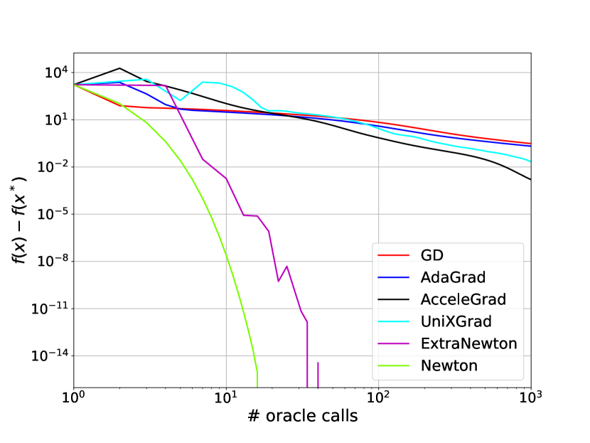
(a) Least-squares regression on a1a

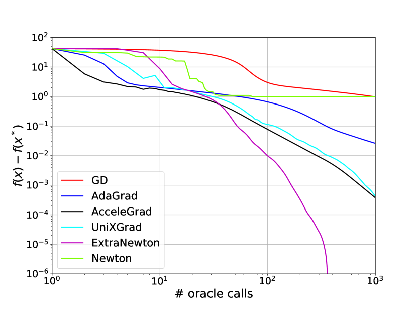
(b) Logistic regression on a1a

Figure 1. Comparison of value convergence for regression problems with deterministic oracle access

For the logistic regression problem, we regularize it with $g(x)=1/2\lVert{x}\rVert^{2}$, but use a very small regularization constant to render the problem ill-conditioned, making things slightly more difficult for the algorithms [47, 49]. Although we implement Newton’s with line-search, we actually observed a sporadic convergence behavior; when the initial point is close to the solution it converges similarly to Extra-Newton, however when we initialize further away it doesn’t converge. This non-convergent behavior has been known for Newton’s, even with line-search present [27]. On the contrary, Extra-Newton consistently converges; even if we perturb the initial step-size and make it adversarially large, it manages to recover due to its adaptive step-size.

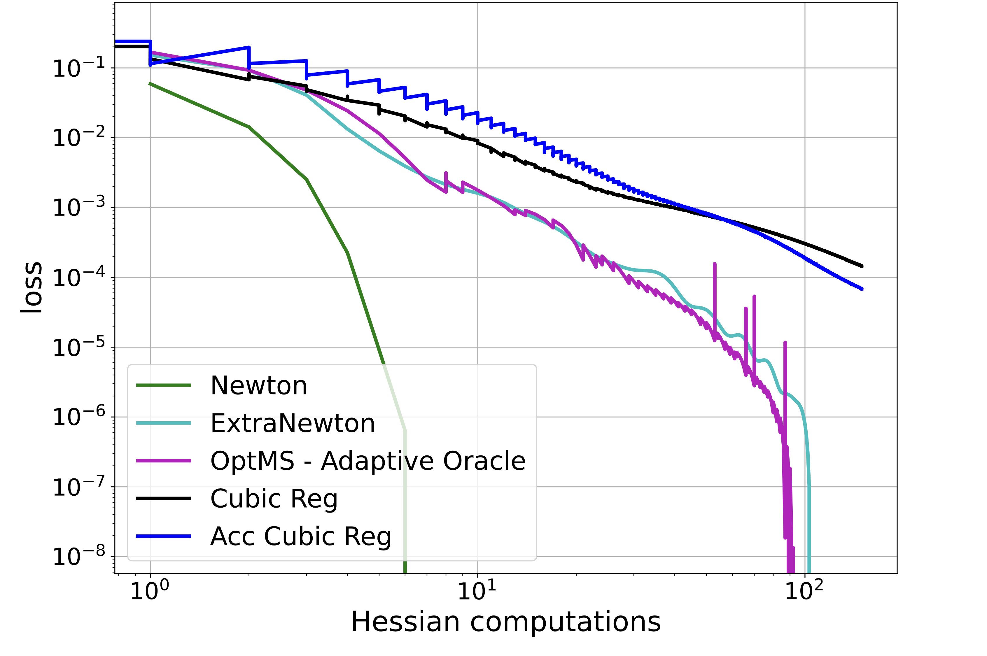
(a) Value convergence w.r.t # Hessian oracle calls

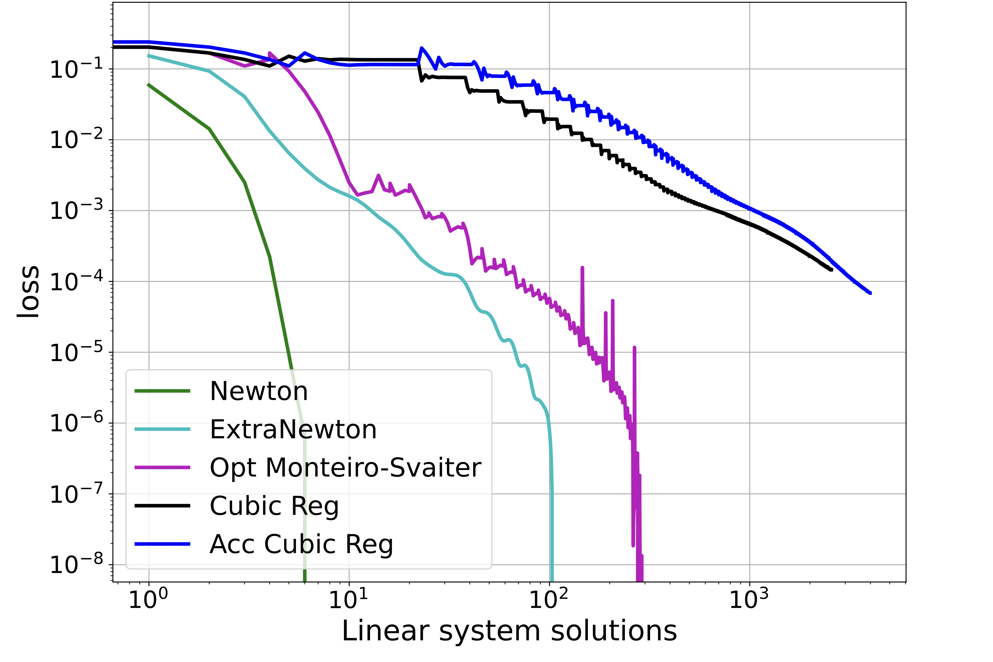
(b) Value convergence w.r.t. # linear system solutions

Figure 2. Extra-Newton vs. second-order methods. Logistic regression with a9a dataset

We complement our numerical tests by comparing Extra-Newton with a set of second-order methods. To that end, we implemented our method within the framework presented in [13]. Using the implementation and the experimental setup provided in their GitHub repository [24], we implemented our method in their code and compared against Newton’s, CRN, ACRN and OptMS algorithms. Figure 2 shows that Extra-Newton has comparable performance to OptMS, which has the theoretically faster rate $O(1/T^{7/2})$, and marginally outperforms with respect to number of linear system solutions since the linesearch procedure of OptMS might require multiple system solutions per iteration. While CRN and ACRN has worse convergence than Extra-Newton, Newton’s seems to have the fastest. Note that the initialization favors Newton’s as it lies in a close neighborhood of the solution, and Newton’s performance sporadically deteriorates when initialized arbitrarily.

5. Conclusion

In this work, we present the first universal, second-order algorithm, Extra-Newton, which enjoys the value convergence rate of $O(\sigma_{g}/\sqrt{T}+\sigma_{H}/T^{3/2}+1/T^{3})$. By extending the notion of bounded variance on stochastic gradients to stochastic Hessian, we prove adaptation to the noise in first and second-order oracles, simultaneously, while showing accelerated rates matching that of Nesterov [55] under the fully deterministic oracle model. To that end, an important open question is whether we could design a method that achieves an improved rate interpolation guarantee $O(\sigma_{g}/\sqrt{T}+\sigma_{H}/T^{3/2}+1/T^{7/2})$ without depending on any line-search/bisection mechanism. We defer this to a future work.

 

APPENDIX

 

Appendix A Preface

In Appendix B, we provide a complete list of notation and definitions that we have used throughout the manuscript.

In Appendix C, we showcase additional numerical evidence for the comparison we provided in the main text. Due to space constraints, we moved most of our plots to the appendix. We investigate the practical behavior in both deterministic and stochastic setting.

In Appendix D, we begin with the proof of the generalized online-to-batch conversion in Theorem 3.3 to form the connection between the offline regret $\textsc{R}_{\textnormal{T}}(x^{\ast})$ and value convergence $f(\bar{X}_{T+\frac{1}{2}})-f(x^{\ast})$.

Then in Appendix E, we present the analysis for obtaining the template regret bound in Proposition 3.1. This template inequality is indeed the point where the analysis in the deterministic, implicit setting and universal, explicit setting part ways.

In Appendix F, we take a small detour to introduce a crucial numerical inequality that is commonly used in the analysis of adaptive methods.

We present the universal convergence analysis of Extra-Newton (Theorem 3.2) in Appendix G.

In Appendix H, we share the analysis of our conceptual framework: convergence of the implicit algorithm (Implicit) in deterministic setting (Theorem 3.1), with the appropriate corollary of Proposition 3.1 for the case of deterministic oracles in this section.

Appendix B Notation and Definitions

To complement the notation in Section 2, we will present a complete list of definitions and parameter descriptions to make it easier for the reader to follow the technical arguments in the whole paper.

Table 2. A complete list of parameters and expressions, their definitions and descriptions

	Formal Definition	Description
$f$	$f:\mathbb{R}^{d}\to\mathbb{R}+\left\{{+\infty}\right\}$	objective function
$\mathcal{X}$	$\mathcal{X}\subset\mathbb{R}^{d}$	convex and compact constraint set
$x^{\ast}$	$=\operatorname*{arg\,min}_{x\in\mathcal{X}}f(x)$	solution of the constrained problem (Opt)
$D$	$=\sup_{x,y\in\mathcal{X}}\lVert{x-y}\rVert$	diameter of the constraint set $\mathcal{X}$
$L$	$\|\nabla^{2}f(x)-\nabla^{2}f(x^{\prime})\|\leq L\|x-x^{\prime}\|$	second-order smoothness constant of $f$
$g(\cdot,\xi)$	$\mathbb{E}\left[\,g(x,\xi)\mid x\,\right]=\nabla f(x)$, $\,\,x\perp\!\!\!\!\perp\xi$	unbiased gradient estimate
$H(\cdot,\xi)$	$\mathbb{E}\left[\,H(x,\xi)\mid x\,\right]=\nabla^{2}f(x)$, $\,\,x\perp\!\!\!\!\perp\xi$	unbiased Hessian estimate
$\mathcal{F}_{t}$	$=\sigma(\xi_{1},\xi_{1+\frac{1}{2}},\cdots,\xi_{t})$	$\sigma$-algebra generated by random variables up to $\xi_{t}$
$\mathcal{F}_{t+\frac{1}{2}}$	$=\sigma(\xi_{1},\xi_{1+\frac{1}{2}},\cdots,\xi_{t},\xi_{t+\frac{1}{2}})$	$\sigma$-algebra generated by random variables up to $\xi_{t+\frac{1}{2}}$
$\sigma_{g}$	$\mathbb{E}\left[\,\lVert{g(x)-\nabla f(x)}\rVert^{2}\mid x\,\right]\leq\sigma_{g}^{2}$	variance bound for gradient estimate
$\sigma_{H}$	$\mathbb{E}\left[\,\lVert{H(x)-\nabla^{2}f(x)}\rVert^{2}\mid x\,\right]\leq\sigma_{H}^{2}$	variance bound for Hessian estimate
$\sigma$	$=\max\left\{{\sigma_{g},\sigma_{H}}\right\}$	maximum variance of oracles
$\gamma_{t}$	Eq. (7) and Eq. (2)	adaptive step-size
$a_{t}$	$=t^{2}$	gradient weights
$A_{t}$	$=\sum_{s=1}^{t}a_{s}$	normalization factor for gradient weights $a_{t}$
$b_{t}$	$=t^{p}$, where $p\geq 2$	averaging weights
$B_{t}$	$=\sum_{s=1}^{t}b_{s}$	normalization factor for averaging weights $b_{t}$

Appendix C Further Experimental Evaluation

In this section we will present additional numerical experiments in two fronts;

• we run logistic regression and least-squares regression under deterministic gradients with another LIBSVM datasets, w1a,

• and subsequently display results in the stochastic setting for the same datasets a1a, w1a.

Figure 3 shows the results for the deterministic experiments while Figure 4 focuses on the results of the stochastic setting. In both figures, we present results for the least-squares in the first column and the logistic regression in the second column.

In Figure 3, the x-axis represent the number of calls made to the deterministic oracle, and in Figure 4, x-axis corresponds to number of full data passes (epochs) to compute the stochastic gradient estimates. The deterministic setup is the same as we described in the main text. In the case of stochastic gradients, we compute mini-batch gradient estimates with a batch-size of 50 samples. We plot the mean of 5 trials for all the methods under mini-batch gradients and also display the variance as the shaded region around the mean curve.

For the case of logistic regression under deterministic gradients, our method performs better than the rest of the pack with a1a dataset but has almost matching performance with a smaller performance gap compared to accelerated first-order methods with w1a dataset. For both datasets, we tried to tune Newton’s method for a randomly-chosen initialization but it was very difficult to find a parameter setting where Newton shows any reasonable behavior. One could notice that Newton’s method doesn’t converge to the solution for logistic regression problem for this random initial point.

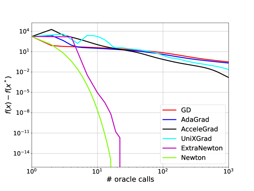
(a) Least-squares, a1a

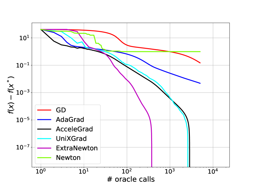
(b) Logistic regression, a1a

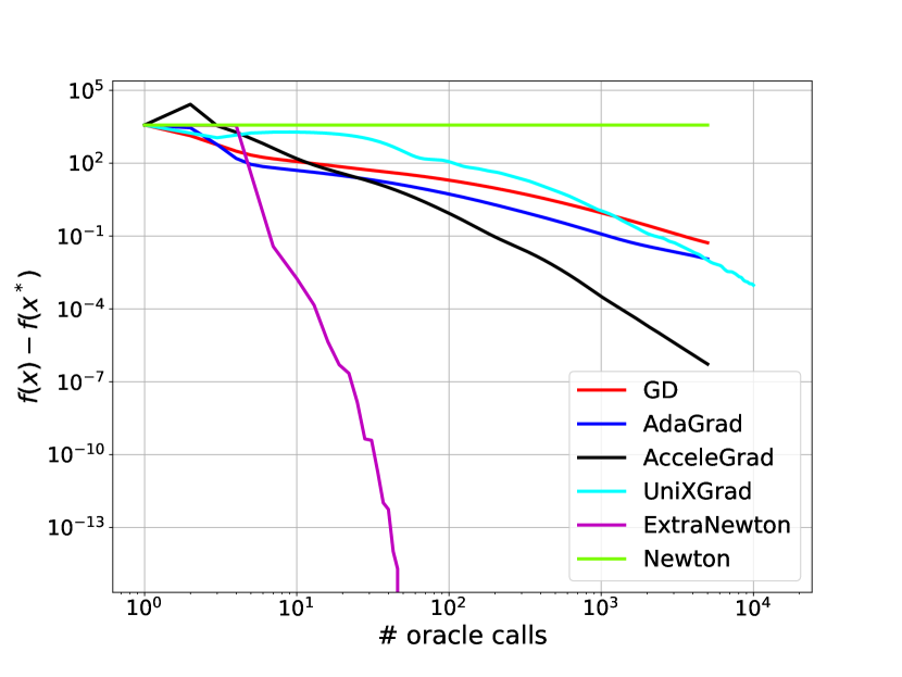
(c) Least-squares, w1a

(d) Logistic regression, w1a

Figure 3. Comparison of value convergence for regression problems with deterministic oracle access

We observe that the main advantage of our approach, and in general that of second-order methods, becomes apparent when the problem at hand has a compatible structure such as least-squares. Intuitively, second-order methods should benefit when the cost of computing the Hessian is comparable to gradient computation. In fact, quadratic problems like least-squares yield a constant Hessian for any point in the domain, granting a significant advantage to second-order methods. We exemplify this behavior for least-squares problem with deterministic oracles. With w1a dataset, we couldn’t get Newton’s method to converge once again. On the contrary, our method shows significant performance upgrade compared to first-order methods while converging consistently in all our trials.

Finally, we have the experiments under stochastic oracles. We essentially present these results for two main reasons; to show that our method works seamlessly with stochastic gradients without any modifications, and to demonstrate that Extra-Newton achieves the $O(1/\sqrt{T})$ rate (same as other methods we compare against) when the gradient information is noisy. We showcase both of these perspectives in Figure 4.

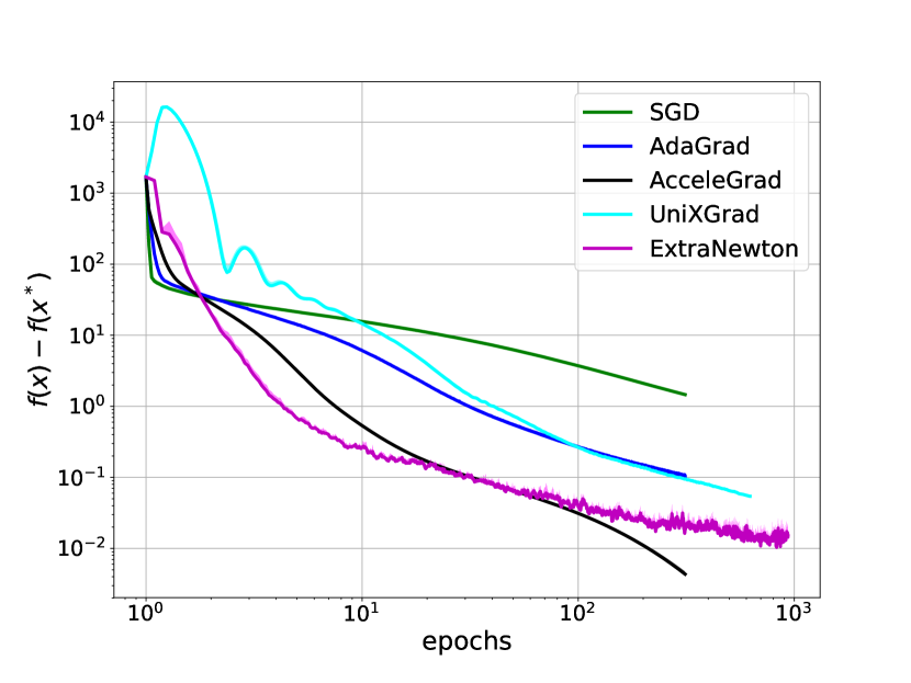
(a) Least-squares, a1a

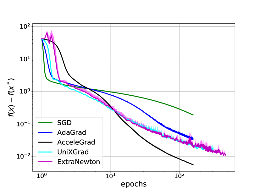
(b) Logistic regression, a1a

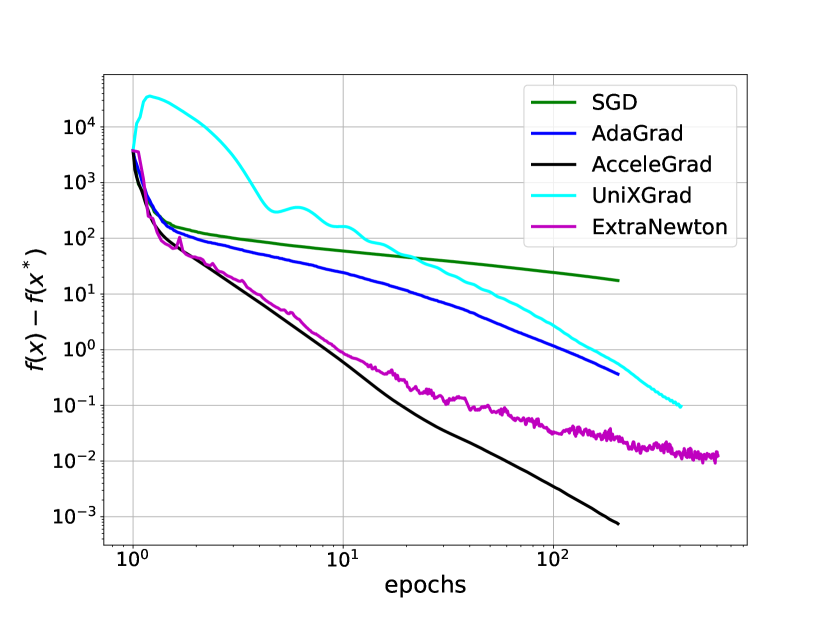
(c) Least-squares, w1a

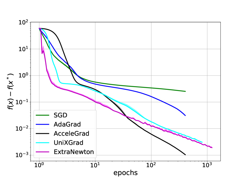
(d) Logistic regression, w1a

Figure 4. Comparison of value convergence for regression problems with stochastic oracle access

Appendix D Generalized Online-to-batch Conversion (Theorem 3.3)

In this section we present the online-to-batch conversion scheme which connects the optimality gap $f(\bar{X}_{T+\frac{1}{2}})-f(x^{\ast})$ with the "weighted" regret $\textsc{R}_{\textnormal{T}}(x^{\ast})=\sum_{t=1}^{T}a_{t}\langle{\nabla f(\bar{X}_{t+\frac{1}{2}})},{X_{t+\frac{1}{2}}-x^{\ast}}\rangle$.

Theorem 3.3.

Let $\textsc{R}_{\textnormal{T}}(x^{\ast})$ denote the anytime regret for the decision sequence $\{X_{t+\frac{1}{2}}\}_{t=1}^{T}$ as in (Reg), and define two sequences of non-decreasing weights $a_{t}$ and $b_{t}$ such that $a_{t},b_{t}\geq 1$. As long as $a_{t}/b_{t}$ is ensured to be non-increasing,

$$f(\bar{X}_{T+\frac{1}{2}})-f(x^{\ast})\leq\frac{\textsc{R}_{\textnormal{T}}(x^{\ast})}{a_{T}\frac{B_{T}}{b_{T}}}$$

Proof.

First, recall the definition of the offline regret:

$$\textsc{R}_{\textnormal{T}}(x^{\ast})=\sum_{t=1}^{T}a_{t}\langle{\nabla f(\bar{X}_{t+\frac{1}{2}}},{X_{t+\frac{1}{2}}-x^{\ast}}\rangle$$

Devising our analysis in the spirit of [18, 35], we need to relate $X_{t+\frac{1}{2}}$ to the average iterate $\bar{X}_{t+\frac{1}{2}}$ in order to exploit the convexity of the objective function. Notice that we could write the iterate $X_{t+\frac{1}{2}}$ as the difference of consecutive average iterates,

$$a_{t}X_{t+\frac{1}{2}}=a_{t}\frac{B_{t}}{b_{t}}\bar{X}_{t+\frac{1}{2}}-a_{t}\frac{B_{t-1}}{b_{t}}\bar{X}_{t-\frac{1}{2}}.$$ (8)

Also, we could subsequently express $a_{t}x^{\ast}=a_{t}\frac{B_{t}}{b_{t}}x^{\ast}-a_{t}\frac{B_{t-1}}{b_{t}}x^{\ast}$. Combining them together,

$$\textsc{R}_{\textnormal{T}}(x^{\ast}) =\sum_{t=1}^{T}a_{t}\langle{\nabla f(\bar{X}_{t+\frac{1}{2}}},{X_{t+\frac{1}{2}}-x^{\ast}}\rangle$$

$$=\sum_{t=1}^{T}a_{t}\frac{B_{t}}{b_{t}}\langle{\nabla f(\bar{X}_{t+\frac{1}{2}})},{\bar{X}_{t+\frac{1}{2}}-x^{\ast}}\rangle-a_{t}\frac{B_{t-1}}{b_{t}}\langle{\nabla f(\bar{X}_{t+\frac{1}{2}}},{\bar{X}_{t-\frac{1}{2}}-x^{\ast}}\rangle$$

$$=\sum_{t=1}^{T}a_{t}\langle{\nabla f(\bar{X}_{t+\frac{1}{2}})},{\bar{X}_{t+\frac{1}{2}}-x^{\ast}}\rangle+a_{t}\frac{B_{t-1}}{b_{t}}\langle{\nabla f(\bar{X}_{t+\frac{1}{2}})},{\bar{X}_{t+\frac{1}{2}}-\bar{X}_{t-\frac{1}{2}}}\rangle$$

where we added and subtracted $a_{t}\frac{B_{t-1}}{b_{t}}\langle{\nabla f(\bar{X}_{t+\frac{1}{2}})},{\bar{X}_{t+\frac{1}{2}}}\rangle$ to obtain the second equality. Having expressed both inner products in the form we want, we could apply convexity and telescope.

$$\sum_{t=1}^{T}a_{t} \langle{\nabla f(\bar{X}_{t+\frac{1}{2}}},{X_{t+\frac{1}{2}}-x^{\ast}}\rangle$$

$$\geq\sum_{t=1}^{T}a_{t}\left({f(\bar{X}_{t+\frac{1}{2}})-f(x^{\ast})}\right)+a_{t}\frac{B_{t-1}}{b_{t}}\left({f(\bar{X}_{t+\frac{1}{2}})-f(\bar{X}_{t-\frac{1}{2}})}\right)$$

$$=\sum_{t=1}^{T}a_{t}\left({f(\bar{X}_{t+\frac{1}{2}})-f(x^{\ast})}\right)+a_{t}\frac{B_{t-1}}{b_{t}}\left({f(\bar{X}_{t+\frac{1}{2}})-f(x^{\ast})}\right)-a_{t}\frac{B_{t-1}}{b_{t}}\left({f(\bar{X}_{t-\frac{1}{2}})-f(x^{\ast})}\right)$$

$$=\sum_{t=1}^{T}a_{t}\frac{B_{t}}{b_{t}}\left({f(\bar{X}_{t+\frac{1}{2}})-f(x^{\ast})}\right)-a_{t}\frac{B_{t-1}}{b_{t}}\left({f(\bar{X}_{t-\frac{1}{2}})-f(x^{\ast})}\right)$$

$$=a_{T}\frac{B_{T}}{b_{T}}\left({f(\bar{X}_{T+\frac{1}{2}})-f(x^{\ast})}\right)-a_{1}\frac{B_{0}}{b_{1}}\left({f(\bar{X}_{-1/2})-f(x^{\ast})}\right)+\sum_{t=1}^{T-1}B_{t}\left({\frac{a_{t}}{b_{t}}-\frac{a_{t+1}}{b_{t+1}}}\right)\left({f(\bar{X}_{t+\frac{1}{2}})-f(x^{\ast})}\right)$$

Setting $B_{0}=0$ eliminates the second term. To conclude the proof, we need to show that the summation term in the above expression is always non-negative. This is ensured when the sequence $\frac{a_{t}}{b_{t}}$ is monotonically non-increasing, which is specified in the theorem statement (and subsequently satisfied by the algorithms). Hence,

$$\sum_{t=1}^{T}a_{t} \langle{\nabla f(\bar{X}_{t+\frac{1}{2}}},{X_{t+\frac{1}{2}}-x^{\ast}}\rangle$$

$$=a_{T}\frac{B_{T}}{b_{T}}\left({f(\bar{X}_{T+\frac{1}{2}})-f(x^{\ast})}\right)+\sum_{t=1}^{T-1}B_{t}\left({\frac{a_{t}}{b_{t}}-\frac{a_{t+1}}{b_{t+1}}}\right)\left({f(\bar{X}_{t+\frac{1}{2}})-f(x^{\ast})}\right)$$

$$\geq a_{T}\frac{B_{T}}{b_{T}}\left({f(\bar{X}_{T+\frac{1}{2}})-f(x^{\ast})}\right).$$

Rearranging the terms gives us the final result

$$f(\bar{X}_{T+\frac{1}{2}})-f(x^{\ast})\leq\frac{\sum_{t=1}^{T}a_{t}\langle{\nabla f(\bar{X}_{t+\frac{1}{2}})},{X_{t+\frac{1}{2}}-x^{\ast}}\rangle}{a_{T}\frac{B_{T}}{b_{T}}}=\frac{\textsc{R}_{\textnormal{T}}(x^{\ast})}{a_{T}\frac{B_{T}}{b_{T}}}.$$

∎

Appendix E Template Regret Bound (Proposition 3.1)

In this section, we will prove the template inequality in Proposition 3.1 in the case of stochastic oracles. This inequality will give us the main departure point for both Theorem 3.1 and Theorem 3.2. We will prove a corollary of the following result later on, specifically for the deterministic setup, which will follow the same steps as Proposition 3.1.

For ease of navigation, we present Extra-Newton once more.

Extra-Newton

Input: $X_{1}\in\mathcal{X}$, $\,a_{t}=t^{2}$ and $A_{t}=\sum_{s=1}^{t}a_{s}$, $\,b_{t}=t^{p}$ ($p\geq 2$) and $B_{t}=\sum_{s=1}^{t}b_{s}$, $\,\gamma>0$, $\xi_{t}\sim$ i.i.d.

1:  for $t=1$ to $T$ do

2:     $~{}~{}~{}~{}~{}~{}\gamma_{t}=\dfrac{\gamma}{\sqrt{\beta_{0}+\sum_{s=1}^{t-1}a_{s}^{2}\lVert{g(\bar{X}_{s+\frac{1}{2}},\xi_{s+\frac{1}{2}})-\mathbf{\tilde{F}}(\bar{X}_{s+\frac{1}{2}};\tilde{X}_{s},\xi_{s})}\rVert^{2}}}$

3:     $X_{t+\frac{1}{2}}=\operatorname*{arg\,min}_{x\in\mathcal{X}}\langle{a_{t}g(\tilde{X}_{t},\xi_{t})},{x}\rangle+\frac{a_{t}b_{t}}{2B_{t}}\langle{H(\tilde{X}_{t},\xi_{t})(x-X_{t})},{x-X_{t}}\rangle+\frac{1}{2\gamma_{t}}\lVert{x-X_{t}}\rVert^{2}$

4:     $\,X_{t+1}=\operatorname*{arg\,min}_{x\in\mathcal{X}}\langle{a_{t}g(\bar{X}_{t+\frac{1}{2}},\xi_{t+\frac{1}{2}})},{x}\rangle+\frac{1}{2\gamma_{t}}\lVert{x-X_{t}}\rVert^{2}$

5:  end for

Proposition 3.1.

Let $\{X_{t+\frac{1}{2}}\}_{t=1}^{T}$ be generated by Algorithm 1, run with a non-increasing step-size sequence $\gamma_{t}$ and non-decreasing sequences of weights $a_{t},b_{t}\geq 1$ such that $a_{t}/b_{t}$ is also non-increasing. Then, the following guarantee holds:

$$\mathbb{E}\textsc{R}_{\textnormal{T}}(x^{\ast})\leq\frac{1}{2}\mathbb{E}\left[\,\frac{3D^{2}}{\gamma_{T+1}}+\sum_{t=1}^{T}\gamma_{t+1}a_{t}^{2}\lVert{g(\bar{X}_{t+\frac{1}{2}},\xi_{t+\frac{1}{2}})-\mathbf{\tilde{F}}(\bar{X}_{t+\frac{1}{2}};\tilde{X}_{t},\xi_{t})}\rVert^{2}-\frac{\lVert{X_{t+\frac{1}{2}}-X_{t}}\rVert^{2}}{\gamma_{t+1}}\,\right]$$

Proof.

We take off from the optimality conditions associated with each update sequence for our explicit algorithm Extra-Newton (Algorithm 1). Optimality condition for $X_{t+\frac{1}{2}}$ implies for any $z_{0}\in\mathcal{X}$,

$$\langle{a_{t}g(\tilde{X}_{t},\xi_{t})+a_{t}\frac{b_{t}}{B_{t}}H(\tilde{X}_{t},\xi_{t})(X_{t+\frac{1}{2}}-X_{t})},{X_{t+\frac{1}{2}}-z_{0}}\rangle$$ (9)

$$=\langle{a_{t}g(\tilde{X}_{t},\xi_{t})+a_{t}H(\tilde{X}_{t},\xi_{t})(\bar{X}_{t+\frac{1}{2}}-\tilde{X}_{t})},{X_{t+\frac{1}{2}}-z_{0}}\rangle$$

$$=\langle{a_{t}\mathbf{\tilde{F}}(\bar{X}_{t+\frac{1}{2}};\tilde{X}_{t},\xi_{t})},{X_{t+\frac{1}{2}}-z_{0}}\rangle$$

$$\leq\frac{1}{\gamma_{t}}\langle{X_{t+\frac{1}{2}}-X_{t}},{z_{0}-X_{t+\frac{1}{2}}}\rangle$$

$$=\frac{1}{2\gamma_{t}}\left({\lVert{X_{t}-z_{0}}\rVert^{2}-\lVert{X_{t+\frac{1}{2}}-z_{0}}\rVert^{2}-\lVert{X_{t+\frac{1}{2}}-X_{t}}\rVert^{2}}\right)$$

Similarly, optimality of $X_{t+1}$ update yields for any $z_{1}\in\mathcal{X}$,

$$\langle{a_{t}g(\bar{X}_{t+\frac{1}{2}},\xi_{t+\frac{1}{2}})},{X_{t+1}-z_{1}}\rangle \leq\frac{1}{2\gamma_{t}}\langle{X_{t+1}-X_{t}},{z_{1}-X_{t+1}}\rangle$$ (10)

$$=\frac{1}{2\gamma_{t}}\left({\lVert{X_{t}-z_{1}}\rVert^{2}-\lVert{X_{t+1}-z_{1}}\rVert^{2}-\lVert{X_{t+1}-X_{t}}\rVert^{2}}\right)$$

First, we will set $z_{1}=x^{\ast}$ to establish the telescoping summation over $\lVert{X_{t}-x^{\ast}}\rVert^{2}-\lVert{X_{t+1}-x^{\ast}}\rVert^{2}$. Then, we will simply align the above expression with the regret as follows,

$$\langle a_{t}g(\bar{X}_{t+\frac{1}{2}},\xi_{t+\frac{1}{2}}), \,X_{t+\frac{1}{2}}-x^{\star}\rangle$$ (11)

$$=\langle{a_{t}g(\bar{X}_{t+\frac{1}{2}},\xi_{t+\frac{1}{2}})},{X_{t+\frac{1}{2}}-X_{t+1}}\rangle+\langle{a_{t}g(\bar{X}_{t+\frac{1}{2}},\xi_{t+\frac{1}{2}})},{X_{t+1}-x^{\star}}\rangle$$

$$\leq\langle{a_{t}g(\bar{X}_{t+\frac{1}{2}},\xi_{t+\frac{1}{2}})},{X_{t+\frac{1}{2}}-X_{t+1}}\rangle$$

$$\quad+\frac{1}{2\gamma_{t}}\left({\lVert{X_{t}-x^{\star}}\rVert^{2}-\lVert{X_{t+1}-x^{\star}}\rVert^{2}-\lVert{X_{t+1}-X_{t}}\rVert^{2}}\right)$$

Now, observe that setting $z_{0}=X_{t+1}$ in Eq. (9) and rearranging we have

$$-\frac{1}{2\gamma_{t}}\lVert{X_{t+1}-X_{t}}\rVert^{2}$$

$$\leq-\langle{a_{t}\mathbf{\tilde{F}}(\bar{X}_{t+\frac{1}{2}};\tilde{X}_{t},\xi_{t})},{X_{t+\frac{1}{2}}-X_{t+1}}\rangle-\frac{1}{2\gamma_{t}}\left({\lVert{X_{t+\frac{1}{2}}-X_{t+1}}\rVert^{2}+\lVert{X_{t+\frac{1}{2}}-X_{t}}\rVert^{2}}\right)$$

Plugging the above expression into Eq. (11) and summing over $t=1,...,T$, we will obtain,

$$\sum_{t=1}^{T} \langle a_{t}g(\bar{X}_{t+\frac{1}{2}},\xi_{t+\frac{1}{2}}),X_{t+\frac{1}{2}}-x^{\star}\rangle$$

$$\leq\sum_{t=1}^{T}a_{t}\langle{g(\bar{X}_{t+\frac{1}{2}},\xi_{t+\frac{1}{2}})-\mathbf{\tilde{F}}(\bar{X}_{t+\frac{1}{2}};\tilde{X}_{t},\xi_{t})},{X_{t+\frac{1}{2}}-X_{t+1}}\rangle$$

$$\quad+\sum_{t=1}^{T}\frac{1}{2\gamma_{t}}\left({\lVert{X_{t}-x^{\star}}\rVert^{2}-\lVert{X_{t+1}-x^{\star}}\rVert^{2}-\lVert{X_{t+\frac{1}{2}}-X_{t+1}}\rVert^{2}-\lVert{X_{t+\frac{1}{2}}-X_{t}}\rVert^{2}}\right)$$

First off, we bound the inner product term using Cauchy-Schwarz and a slight generalization of Young’s inequality [63]

$$\sum_{t=1}^{T} \,a_{t}\langle{g(\bar{X}_{t+\frac{1}{2}},\xi_{t+\frac{1}{2}})-\mathbf{\tilde{F}}(\bar{X}_{t+\frac{1}{2}};\tilde{X}_{t},\xi_{t})},{X_{t+\frac{1}{2}}-X_{t+1}}\rangle$$

$$\leq\sum_{t=1}^{T}a_{t}\lVert{g(\bar{X}_{t+\frac{1}{2}},\xi_{t+\frac{1}{2}})-\mathbf{\tilde{F}}(\bar{X}_{t+\frac{1}{2}};\tilde{X}_{t},\xi_{t})}\rVert\lVert{X_{t+\frac{1}{2}}-X_{t+1}}\rVert$$

$$\leq\frac{1}{2}\sum_{t=1}^{T}\gamma_{t+1}a_{t}^{2}\lVert{g(\bar{X}_{t+\frac{1}{2}},\xi_{t+\frac{1}{2}})-\mathbf{\tilde{F}}(\bar{X}_{t+\frac{1}{2}};\tilde{X}_{t},\xi_{t})}\rVert^{2}+\frac{1}{\gamma_{t+1}}\lVert{X_{t+\frac{1}{2}}-X_{t+1}}\rVert^{2}.$$

We merge the expressions together,

$$\sum_{t=1}^{T} \langle a_{t}g(\bar{X}_{t+\frac{1}{2}},\xi_{t+\frac{1}{2}}),X_{t+\frac{1}{2}}-x^{\star}\rangle$$

$$\leq\frac{1}{2}\sum_{t=1}^{T}\gamma_{t+1}a_{t}^{2}\lVert{g(\bar{X}_{t+\frac{1}{2}},\xi_{t+\frac{1}{2}})-\mathbf{\tilde{F}}(\bar{X}_{t+\frac{1}{2}};\tilde{X}_{t},\xi_{t})}\rVert^{2}+\frac{1}{\gamma_{t+1}}\lVert{X_{t+\frac{1}{2}}-X_{t+1}}\rVert^{2}$$

$$\quad+\sum_{t=1}^{T}\frac{1}{2\gamma_{t}}\left({\lVert{X_{t}-x^{\star}}\rVert^{2}-\lVert{X_{t+1}-x^{\star}}\rVert^{2}-\lVert{X_{t+\frac{1}{2}}-X_{t+1}}\rVert^{2}-\lVert{X_{t+\frac{1}{2}}-X_{t}}\rVert^{2}}\right)$$

It is important that we invoke generalized Young’s inequality with step-size at time $t+1$. Since the step-size lags one iteration behind, $\gamma_{t}$ does not include $\lVert{g(\bar{X}_{t+\frac{1}{2}},\xi_{t+\frac{1}{2}})-\mathbf{\tilde{F}}(\bar{X}_{t+\frac{1}{2}};\tilde{X}_{t},\xi_{t})}\rVert^{2}$ and this would pose some problems in the later stages of the proof. Hence, we add/subtract $\frac{1}{\gamma_{t+1}}\lVert{X_{t+\frac{1}{2}}-X_{t}}\rVert^{2}$ and regroup the terms,

$$\sum_{t=1}^{T} \langle a_{t}g(\bar{X}_{t+\frac{1}{2}},\xi_{t+\frac{1}{2}}),X_{t+\frac{1}{2}}-x^{\star}\rangle$$

$$\leq\frac{1}{2}\sum_{t=1}^{T}\gamma_{t+1}a_{t}^{2}\lVert{g(\bar{X}_{t+\frac{1}{2}},\xi_{t+\frac{1}{2}})-\mathbf{\tilde{F}}(\bar{X}_{t+\frac{1}{2}};\tilde{X}_{t},\xi_{t})}\rVert^{2}-\frac{1}{\gamma_{t+1}}\lVert{X_{t+\frac{1}{2}}-X_{t}}\rVert^{2}$$

$$\quad+\frac{1}{2}\sum_{t=1}^{T}\left({\frac{1}{\gamma_{t+1}}-\frac{1}{\gamma_{t}}}\right)\left({\lVert{X_{t+\frac{1}{2}}-X_{t+1}}\rVert^{2}+\lVert{X_{t+\frac{1}{2}}-X_{t}}\rVert^{2}}\right)$$

$$\quad+\frac{1}{2}\sum_{t=1}^{T}\frac{1}{\gamma_{t}}\left({\lVert{X_{t}-x^{\star}}\rVert^{2}-\lVert{X_{t+1}-x^{\star}}\rVert^{2}}\right)$$

$$\leq\frac{1}{2}\sum_{t=1}^{T}\gamma_{t+1}a_{t}^{2}\lVert{g(\bar{X}_{t+\frac{1}{2}},\xi_{t+\frac{1}{2}})-\mathbf{\tilde{F}}(\bar{X}_{t+\frac{1}{2}};\tilde{X}_{t},\xi_{t})}\rVert^{2}-\frac{1}{\gamma_{t+1}}\lVert{X_{t+\frac{1}{2}}-X_{t}}\rVert^{2}$$

$$\quad+\frac{\lVert{X_{1}-x^{\ast}}\rVert^{2}}{2\gamma_{1}}+\frac{1}{2}\sum_{t=1}^{T-1}\left({\frac{1}{\gamma_{t+1}}-\frac{1}{\gamma_{t}}}\right)\lVert{X_{t+1}-x^{\star}}\rVert^{2}+D^{2}\sum_{t=1}^{T}\left({\frac{1}{\gamma_{t+1}}-\frac{1}{\gamma_{t}}}\right)$$

$$\leq\frac{3D^{2}}{2\gamma_{T+1}}+\frac{1}{2}\sum_{t=1}^{T}\gamma_{t+1}a_{t}^{2}\lVert{g(\bar{X}_{t+\frac{1}{2}},\xi_{t+\frac{1}{2}})-\mathbf{\tilde{F}}(\bar{X}_{t+\frac{1}{2}};\tilde{X}_{t},\xi_{t})}\rVert^{2}-\frac{1}{2}\sum_{t=1}^{T}\frac{1}{\gamma_{t+1}}\lVert{X_{t+\frac{1}{2}}-X_{t}}\rVert^{2}$$

where we have rewritten the telescoping summation for $\lVert{X_{t}-x^{\star}}\rVert^{2}-\lVert{X_{t+1}-x^{\star}}\rVert^{2}$ and used that $D^{2}=\sup_{x,y\in\mathcal{X}}\lVert{x-y}\rVert^{2}$ (diameter of the constraint set) to obtain the second inequality. The final line follows from telescoping the summations, plugging in the diameter $D$ and rearranging the resulting terms.

Now, what remains is to obtain the (expected) regret from $\sum_{t=1}^{T}\langle a_{t}g(\bar{X}_{t+\frac{1}{2}},\xi_{t+\frac{1}{2}}),X_{t+\frac{1}{2}}-x^{\star}\rangle$. Recall the definitions of $\mathcal{F}_{t}=\sigma(\xi_{1},\xi_{1+\frac{1}{2}},\cdots,\xi_{t})$ and $\mathcal{F}_{t+\frac{1}{2}}=\sigma(\xi_{1},\xi_{1+\frac{1}{2}},\cdots,\xi_{t},\xi_{t+\frac{1}{2}})$ from Table LABEL:tbl:app_notation. Taking expectation over all randomness,

$$\mathbb{E}\Bigg{[}\sum_{t=1}^{T}\langle a_{t}g(\bar{X}_{t+\frac{1}{2}},\xi_{t+\frac{1}{2}}),X_{t+\frac{1}{2}}-x^{\star}\rangle\Bigg{]}$$

$$=\mathbb{E}\left[\,\sum_{t=1}^{T}a_{t}\langle g(\bar{X}_{t+\frac{1}{2}},\xi_{t+\frac{1}{2}})-\nabla f(\bar{X}_{t+\frac{1}{2}}),X_{t+\frac{1}{2}}-x^{\star}\rangle+a_{t}\langle\nabla f(\bar{X}_{t+\frac{1}{2}}),X_{t+\frac{1}{2}}-x^{\star}\rangle\,\right]$$

$$=\mathbb{E}\left[\,\sum_{t=1}^{T}\mathbb{E}\left[\,a_{t}\langle g(\bar{X}_{t+\frac{1}{2}},\xi_{t+\frac{1}{2}})-\nabla f(\bar{X}_{t+\frac{1}{2}}),X_{t+\frac{1}{2}}-x^{\star}\rangle\mid\mathcal{F}_{t}\,\right]\,\right]$$

$$\quad+\mathbb{E}\left[\,\sum_{t=1}^{T}a_{t}\langle\nabla f(\bar{X}_{t+\frac{1}{2}}),X_{t+\frac{1}{2}}-x^{\star}\rangle\,\right]$$

$$=\mathbb{E}\left[\,\sum_{t=1}^{T}a_{t}\langle\mathbb{E}\left[\,g(\bar{X}_{t+\frac{1}{2}},\xi_{t+\frac{1}{2}})\mid\mathcal{F}_{t}\,\right]-\nabla f(\bar{X}_{t+\frac{1}{2}}),X_{t+\frac{1}{2}}-x^{\star}\rangle\,\right]$$

$$\quad+\mathbb{E}\left[\,\sum_{t=1}^{T}a_{t}\langle\nabla f(\bar{X}_{t+\frac{1}{2}}),X_{t+\frac{1}{2}}-x^{\star}\rangle\,\right]$$

$$=\mathbb{E}\left[\,\sum_{t=1}^{T}a_{t}\langle\nabla f(\bar{X}_{t+\frac{1}{2}}),X_{t+\frac{1}{2}}-x^{\star}\rangle\,\right]$$

We used towering property of expectation (equivalently total law of expectation) to have the second inequality, and the last line from the unbiasedness assumption of gradient oracles in Eq. (2) such that $\mathbb{E}\left[\,g(\bar{X}_{t+\frac{1}{2}},\xi_{t+\frac{1}{2}})\mid\mathcal{F}_{t}\,\right]=\nabla f(\bar{X}_{t+\frac{1}{2}})$. Hence, we obtain that

$$\mathbb{E}\left[\,\textsc{R}_{\textnormal{T}}(x^{\ast})\,\right] =\mathbb{E}\left[\,\sum_{t=1}^{T}a_{t}\langle\nabla f(\bar{X}_{t+\frac{1}{2}}),X_{t+\frac{1}{2}}-x^{\star}\rangle\,\right]$$

$$=\mathbb{E}\Bigg{[}\sum_{t=1}^{T}\langle a_{t}g(\bar{X}_{t+\frac{1}{2}},\xi_{t+\frac{1}{2}}),X_{t+\frac{1}{2}}-x^{\star}\rangle\Bigg{]},$$

which concludes the target result,

$$\mathbb{E}\left[\,\textsc{R}_{\textnormal{T}}(x^{\ast})\,\right]\leq\frac{1}{2}\mathbb{E}\left[\,\frac{3D^{2}}{\gamma_{T+1}}+\sum_{t=1}^{T}\gamma_{t+1}a_{t}^{2}\lVert{g(\bar{X}_{t+\frac{1}{2}},\xi_{t+\frac{1}{2}})-\mathbf{\tilde{F}}(\bar{X}_{t+\frac{1}{2}};\tilde{X}_{t},\xi_{t})}\rVert^{2}-\frac{\lVert{X_{t+\frac{1}{2}}-X_{t}}\rVert^{2}}{\gamma_{t+1}}\,\right]$$

∎

Appendix F Technical Lemma for the Main Proofs

Before proceeding with the proofs of our main results, we need to establish the following technical result, due to [48] and [41], which has been commonly used in the analysis of adaptive methods. We make use of it for the proof of Theorem 3.1 and Theorem 3.2.

Lemma F.1 (48, 41).

For all non-negative numbers $\alpha_{1},\dotsc\alpha_{t}$, the following inequality holds:

$$\sqrt{\sum_{t=1}^{T}\alpha_{t}}\leq\sum_{t=1}^{T}\dfrac{\alpha_{t}}{\sqrt{\sum_{i=1}^{t}\alpha_{i}}}\leq 2\sqrt{\sum_{t=1}^{T}\alpha_{t}}$$ (12)

Appendix G Extra-Newton: The First Universal Second-order Accelerated Method (Theorem 3.2)

Theorem 3.2.

Let $\{X_{t+\frac{1}{2}}\}_{t=1}^{T}$ be a sequence generated by Algorithm 1, run with the adaptive step-size policy (2) and $a_{t}=t^{2},b_{t}=t^{p}$ for $p\geq 2$. Assume that $f$ satisfies (H-smooth), and that Assumptions (2) hold . Then, the following universal guarantee holds:

$$f(\bar{X}_{T+\frac{1}{2}})-f(x^{\ast})\leq O\left({\frac{{\frac{D^{2}+\gamma^{2}}{\gamma}}\sigma_{g}}{\sqrt{T}}+\frac{{\frac{D^{3}+D\gamma^{2}}{\gamma}}\sigma_{H}}{T^{3/2}}+\frac{\max\left\{{L{\frac{D^{4}+D\gamma^{3}}{\gamma}},\sqrt{\beta_{0}}{\frac{D^{2}+\gamma^{2}}{\gamma}}}\right\}}{T^{3}}}\right)$$

When $\gamma=D$, we obtain the target rate $O\left({\frac{D\sigma_{g}}{\sqrt{T}}+\frac{D^{2}\sigma_{H}}{T^{3/2}}+\frac{\max\left\{{LD^{3},\sqrt{\beta_{0}}D}\right\}}{T^{3}}}\right)$.

Proof.

We take Proposition 3.1 as our departure point for the analysis. After proving an offline regret bound, we will use Theorem 3.3 to obtain the optimality gap from the regret bound. Recall the template regret bound,

$$\mathbb{E}\textsc{R}_{\textnormal{T}}(x^{\ast})\leq\frac{1}{2}\mathbb{E}\left[\,\frac{3D^{2}}{\gamma_{T+1}}+\sum_{t=1}^{T}\gamma_{t+1}a_{t}^{2}\lVert{g(\bar{X}_{t+\frac{1}{2}},\xi_{t+\frac{1}{2}})-\mathbf{\tilde{F}}(\bar{X}_{t+\frac{1}{2}};\tilde{X}_{t},\xi_{t})}\rVert^{2}-\frac{\lVert{X_{t+\frac{1}{2}}-X_{t}}\rVert^{2}}{\gamma_{t+1}}\,\right]$$

Now, we want to unify the first two terms through numerical inequalities. We will write the second term in terms of the first term. Due to Lemma F.1, we can upper the bound second term as,

$$\frac{1}{2}\sum_{t=1}^{T}\gamma_{t+1}a_{t}^{2} \lVert{g(\bar{X}_{t+\frac{1}{2}},\xi_{t+\frac{1}{2}})-\mathbf{\tilde{F}}(\bar{X}_{t+\frac{1}{2}};\tilde{X}_{t},\xi_{t})}\rVert^{2}$$

$$=\frac{\gamma}{2}\sum_{t=1}^{T}\frac{a_{t}^{2}\lVert{g(\bar{X}_{t+\frac{1}{2}},\xi_{t+\frac{1}{2}})-\mathbf{\tilde{F}}(\bar{X}_{t+\frac{1}{2}};\tilde{X}_{t},\xi_{t})}\rVert^{2}}{\sqrt{\beta_{0}+\sum_{s=1}^{t}a_{s}^{2}\lVert{g(\bar{X}_{s+\frac{1}{2}},\xi_{s+\frac{1}{2}})-\mathbf{\tilde{F}}(\bar{X}_{s+\frac{1}{2}};\tilde{X}_{s},\xi_{s})}\rVert^{2}}}$$

$$\leq\gamma\sqrt{\beta_{0}+\sum_{t=1}^{T}a_{t}^{2}\lVert{g(\bar{X}_{t+\frac{1}{2}},\xi_{t+\frac{1}{2}})-\mathbf{\tilde{F}}(\bar{X}_{t+\frac{1}{2}};\tilde{X}_{t},\xi_{t})}\rVert^{2}}-\frac{\gamma}{2\sqrt{\beta_{0}}}$$

Plugging this back into the original expression gives us

$$\mathbb{E}\left[\,\textsc{R}_{\textnormal{T}}(x^{\ast})\,\right]$$

$$\leq\left({\frac{3D^{2}}{2\gamma}+\gamma}\right)\sqrt{\beta_{0}+\sum_{t=1}^{T}a_{t}^{2}\lVert{g(\bar{X}_{t+\frac{1}{2}},\xi_{s})-\mathbf{\tilde{F}}(\bar{X}_{t+\frac{1}{2}};\tilde{X}_{t},\xi_{t})}\rVert^{2}}-\frac{1}{2}\sum_{t=1}^{T}\frac{1}{\gamma_{t+1}}\lVert{X_{t+\frac{1}{2}}-X_{t}}\rVert^{2}$$

Next up, we will handle the negative term in the above expression. As we have discussed in the main text, the key for faster rates beyond $O(1/T^{2})$ is understanding how to manipulate the negative term in the above expression. A crucial part of our analysis is understanding the implications of second-order smoothness and how to unlock its potential. This next derivation will demonstrate how (H-smooth) allows for a more aggressive gradient weighting and in turn faster convergence rate implied by our generalized conversion technique. Next, we will relate the negative term to the positive terms using smoothness and primal averaging, similar to the approaches in [67, 35].

$$-\frac{\lVert{X_{t+\frac{1}{2}}-X_{t}}\rVert^{2}}{\gamma_{t+1}} =-\frac{D^{2}}{D^{2}\gamma_{t+1}}\lVert{X_{t+\frac{1}{2}}-X_{t}}\rVert^{2}$$

$$\leq-\frac{1}{D^{2}\gamma_{t+1}}\lVert{X_{t+\frac{1}{2}}-X_{t}}\rVert^{4}$$

$$=-\frac{1}{D^{2}\gamma_{t+1}}\frac{B_{t}^{4}}{b_{t}^{4}}\lVert{\frac{b_{t}}{B_{t}}X_{t+\frac{1}{2}}-\frac{b_{t}}{B_{t}}X_{t}}\rVert^{4}$$

$$=-\frac{1}{D^{2}\gamma_{t+1}}\frac{B_{t}^{4}}{b_{t}^{4}}\lVert{\frac{b_{t}X_{t+\frac{1}{2}}+\sum_{s=1}^{t-1}b_{s}X_{s+\frac{1}{2}}}{B_{t}}-\frac{b_{t}X_{t}+\sum_{s=1}^{t-1}b_{s}X_{s+\frac{1}{2}}}{B_{t}}}\rVert^{4}$$

$$=-\frac{1}{D^{2}\gamma_{t+1}}c^{4}t^{4}\lVert{\bar{X}_{t+\frac{1}{2}}-\tilde{X}_{t}}\rVert^{4}$$

$$\leq-\frac{4c^{4}t^{4}}{L^{2}D^{2}\gamma_{t+1}}\lVert{\nabla f(\bar{X}_{t+\frac{1}{2}})-\mathbf{F}(\bar{X}_{t+\frac{1}{2}};\tilde{X}_{t})}\rVert^{2}$$

First, notice that for any sequence $b_{t}=O(t^{p})$ with $p\geq 0$, we have $B_{t}=\sum_{s=1}^{t}b_{s}=O(t^{p+1})$, which implies $\frac{B_{t}}{b_{t}}\leq ct$, where $c>0$ is an absolute constant depending on how $b_{t}$ is defined. Then, we use the definitions of average sequences $\bar{X}_{t+\frac{1}{2}}$ and $\tilde{X}_{t}$ to go from $\lVert{X_{t+\frac{1}{2}}-X_{t}}\rVert^{4}$ to $\lVert{\bar{X}_{t+\frac{1}{2}}-\tilde{X}_{t}}\rVert^{4}$ to obtain equalities 3-5, and apply smoothness to obtain the last line. On a related note, we want to highlight the importance of optimistic weighted averaging that is central for obtaining the above expression. Since the averaged pairs $\bar{X}_{t+\frac{1}{2}}$ and $\tilde{X}_{t}$ differ by only the last element, we can seamlessly relate $\lVert{X_{t+\frac{1}{2}}-X_{t}}\rVert$ to $\lVert{\bar{X}_{t+\frac{1}{2}}-\tilde{X}_{t}}\rVert$.

Now, we are at a position to explain how we will go beyond $O(1/T^{2})$ convergence rate, which fundamentally depends on the gradient weights $a_{t}$ and jointly relies on our generalized online-to-batch conversion in Theorem 3.3. The negative term above is monotonically decreasing (increases in magnitude) which is essential to (partially) control the growth of remaining positive term. More specifically, one can notice that in order to align the summands of the positive and negative term, the algebra dictates that we need to select $a_{t}=O(t^{2})$, which implies $b_{t}=\Omega(t^{2})$. Notice that our averaging and weighting parameters grow at least $O(t)$ faster than the existing accelerated schemes for first-order smoothness, which grants the improved $O(1/T^{3})$ rate. On the contrary, first-order smoothness would only allow $t^{2}$ factor in front of the norm, leading to the slower rate.

Due to (margin-wise) space constraints, we will use a slightly more compact notation for certain expressions. Let us first define a shorthand notation for noise in gradient and Hessian evaluations, respectively.

$$\epsilon_{t} =[g(\bar{X}_{t+\frac{1}{2}},\xi_{t+\frac{1}{2}})-g(\tilde{X}_{t},\xi_{t})]-[\nabla f(\bar{X}_{t+\frac{1}{2}})-\nabla f(\tilde{X}_{t})]$$ (13)

$$\delta_{t} =H(\tilde{X}_{t},\xi_{t})-\nabla^{2}f(\tilde{X}_{t})$$

Then, we define following deterministic/stochastic placeholders:

$$\nabla_{t} =\nabla f(\bar{X}_{t+\frac{1}{2}})-\mathbf{F}(\bar{X}_{t+\frac{1}{2}},\tilde{X}_{t})$$ (14)

$$\widetilde{\nabla}_{t} =g(\bar{X}_{t+\frac{1}{2}},\xi_{t+\frac{1}{2}})-\mathbf{\tilde{F}}(\bar{X}_{t+\frac{1}{2}},\tilde{X}_{t},\xi_{t})=\nabla_{t}+\epsilon_{t}-\delta_{t}(\bar{X}_{t+\frac{1}{2}}-\tilde{X}_{t})$$

Setting $a_{t}=t^{2}$, combining all the terms and introducing the compact notation,

$$\sum_{t=1}^{T}\langle a_{t}g(\bar{X}_{t+\frac{1}{2}},\xi_{t+\frac{1}{2}}),X_{t+\frac{1}{2}}-x^{\star}\rangle$$

$$\leq\left({\frac{3D^{2}}{2\gamma}+\gamma}\right)\sqrt{\beta_{0}+\sum_{t=1}^{T}a_{t}^{2}\lVert{\widetilde{\nabla}_{t}}\rVert^{2}}-\sum_{t=1}^{T}\frac{2c^{4}}{L^{2}D^{2}\gamma_{t+1}}a_{t}^{2}\lVert{\nabla_{t}}\rVert^{2}$$

At this point, we need to understand how to relate $\lVert{\nabla_{t}}\rVert^{2}$ and $\lVert{\widetilde{\nabla}_{t}}\rVert^{2}$ while treating the step-size $\gamma_{t+1}$ accordingly. The issue is that the step-size is agnostic to deterministic oracle information since we accumulate $\lVert{\widetilde{\nabla}_{t}}\rVert^{2}$. From the perspective of step-size, we need to find a relevant, if not matching, lower bound for $\lVert{\nabla_{t}}\rVert^{2}$ and $\lVert{\widetilde{\nabla}_{t}}\rVert^{2}$. Indeed, we follow the ideas presented in [35], and begin by (trivially) lower bounding both terms with the same expression,

$$\lVert{\widetilde{\nabla}_{t}}\rVert^{2} \geq\min\left\{{\lVert{\widetilde{\nabla}_{t}}\rVert^{2},\lVert{\nabla_{t}}\rVert^{2}}\right\}$$ (15)

$$\lVert{\nabla_{t}}\rVert^{2} \geq\min\left\{{\lVert{\widetilde{\nabla}_{t}}\rVert^{2},\lVert{\nabla_{t}}\rVert^{2}}\right\}$$

Now, we will decompose $\lVert{\widetilde{\nabla}_{t}}\rVert^{2}$ into $\lVert{\nabla_{t}}\rVert^{2}$ and the noise terms. Using the definitions in Eq. (13) and (14) and applying triangular inequality with quadratic expansion,

$$\lVert{\widetilde{\nabla}_{t}}\rVert^{2}\leq 2\lVert{\nabla_{t}}\rVert^{2}+4\lVert{\delta_{t}(\bar{X}_{t+\frac{1}{2}}-\tilde{X}_{t})}\rVert^{2}+4\lVert{\epsilon_{t}}\rVert^{2}$$ (16)

We can also have the following trivial upper bound,

$$\lVert{\widetilde{\nabla}_{t}}\rVert^{2} \leq 2\lVert{\widetilde{\nabla}_{t}}\rVert^{2}$$ (17)

$$\leq 2\lVert{\widetilde{\nabla}_{t}}\rVert^{2}+4\lVert{\delta_{t}(\bar{X}_{t+\frac{1}{2}}-\tilde{X}_{t})}\rVert^{2}+4\lVert{\epsilon_{t}}\rVert^{2}$$

Let us simplify the relationship between the bounds in Eq. (16) and Eq. (17); if $\lVert{\nabla_{t}}\rVert^{2}\leq\lVert{\widetilde{\nabla}_{t}}\rVert^{2}$, then Eq. (16) is tighter, otherwise Eq. (17) is tighter. Hence, we could select the minimum of $\lVert{\nabla_{t}}\rVert^{2}$ and $\lVert{\widetilde{\nabla}_{t}}\rVert$:

$$\lVert{\widetilde{\nabla}_{t}}\rVert^{2}\leq 2\min\left\{{\lVert{\widetilde{\nabla}_{t}}\rVert^{2},\lVert{\nabla_{t}}\rVert^{2}}\right\}+4\lVert{\delta_{t}(\bar{X}_{t+\frac{1}{2}}-\tilde{X}_{t})}\rVert^{2}+4\lVert{\epsilon_{t}}\rVert^{2}$$ (18)

Using this intuition, we can construct a variable $\lambda_{t}$ that always upper bounds the step-size.

$$\lambda_{t}=\frac{\gamma}{\sqrt{\beta_{0}+\sum_{s=1}^{t-1}a_{s}^{2}\min\left\{{\lVert{\widetilde{\nabla}_{s}}\rVert^{2},\lVert{\nabla_{s}}\rVert^{2}}\right\}}}$$ (19)

It is immediate that $\gamma_{t}\leq\lambda_{t}$. Essentially, we will replace the terms $\lVert{\nabla_{t}}\rVert^{2}$ and $\lVert{\widetilde{\nabla}_{t}}\rVert^{2}$ with $\min\left\{{\lVert{\widetilde{\nabla}_{t}}\rVert^{2},\lVert{\nabla_{t}}\rVert^{2}}\right\}$, $\lVert{\delta_{t}(\bar{X}_{t+\frac{1}{2}}-\tilde{X}_{t})}\rVert^{2}$ and $\lVert{\epsilon_{t}}\rVert^{2}$.

$$\mathbb{E}\left[\,\textsc{R}_{\textnormal{T}}(x^{\ast})\,\right]$$

$$\leq\mathbb{E}\Bigg{[}{\frac{3D^{2}+2\gamma^{2}}{{2}\gamma}}\sqrt{\beta_{0}+\sum_{t=1}^{T}a_{t}^{2}\lVert{\widetilde{\nabla}_{t}}\rVert^{2}}-\sum_{t=1}^{T}\frac{2c^{4}}{L^{2}D^{2}\gamma_{t+1}}a_{t}^{2}\lVert{\nabla_{t}}\rVert^{2}\Bigg{]}$$

$$\leq\mathbb{E}\Bigg{[}{\frac{3D^{2}+2\gamma^{2}}{{2}\gamma}}\sqrt{\beta_{0}+\sum_{t=1}^{T}2a_{t}^{2}\min\left\{{\lVert{\widetilde{\nabla}_{t}}\rVert^{2},\lVert{\nabla_{t}}\rVert^{2}}\right\}+4a_{t}^{2}\lVert{\delta_{t}(\bar{X}_{t+\frac{1}{2}}-\tilde{X}_{t})}\rVert^{2}+4a_{t}^{2}\lVert{\epsilon_{t}}\rVert^{2}}$$

$$\quad-\sum_{t=1}^{T}\frac{2c^{4}}{L^{2}D^{2}\lambda_{t+1}}a_{t}^{2}\min\left\{{\lVert{\widetilde{\nabla}_{t}}\rVert^{2},\lVert{\nabla_{t}}\rVert^{2}}\right\}\Bigg{]}$$

$$\leq\mathbb{E}\Bigg{[}{\frac{3D^{2}+2\gamma^{2}}{\sqrt{2}\gamma}}\sqrt{\beta_{0}+\sum_{t=1}^{T}a_{t}^{2}\min\left\{{\lVert{\widetilde{\nabla}_{t}}\rVert^{2},\lVert{\nabla_{t}}\rVert^{2}}\right\}}-\sum_{t=1}^{T}\frac{2c^{4}a_{t}^{2}}{L^{2}D^{2}\lambda_{t+1}}\min\left\{{\lVert{\widetilde{\nabla}_{t}}\rVert^{2},\lVert{\nabla_{t}}\rVert^{2}}\right\}$$

$$\quad+2\left({\frac{3D^{2}}{2\gamma}+\gamma}\right)\sqrt{\sum_{t=1}^{T}a_{t}^{2}\lVert{\delta_{t}(\bar{X}_{t+\frac{1}{2}}-\tilde{X}_{t})}\rVert^{2}}+2\left({\frac{3D^{2}}{2\gamma}+\gamma}\right)\sqrt{\sum_{t=1}^{T}a_{t}^{2}\lVert{\epsilon_{t}}\rVert^{2}}~{}~{}\Bigg{]}$$

$$\leq\mathbb{E}\Bigg{[}{\frac{3D^{2}+2\gamma^{2}}{\sqrt{2}\gamma^{2}}}\left({\gamma\sqrt{\beta_{0}}+\sum_{t=1}^{T}\lambda_{t+1}a_{t}^{2}\min\left\{{\lVert{\widetilde{\nabla}_{t}}\rVert^{2},\lVert{\nabla_{t}}\rVert^{2}}\right\}}\right)-\sum_{t=1}^{T}\frac{2c^{4}a_{t}^{2}}{L^{2}D^{2}\lambda_{t+1}}\min\left\{{\lVert{\widetilde{\nabla}_{t}}\rVert^{2},\lVert{\nabla_{t}}\rVert^{2}}\right\}$$

$$\quad+2\left({\frac{3D^{2}}{2\gamma}+\gamma}\right)\sqrt{\sum_{t=1}^{T}a_{t}^{2}\lVert{\delta_{t}(\bar{X}_{t+\frac{1}{2}}-\tilde{X}_{t})}\rVert^{2}}+2\left({\frac{3D^{2}}{2\gamma}+\gamma}\right)\sqrt{\sum_{t=1}^{T}a_{t}^{2}\lVert{\epsilon_{t}}\rVert^{2}}~{}~{}\Bigg{]}$$

$$\leq{\frac{3D^{2}+2\gamma^{2}}{\sqrt{2}\gamma}\sqrt{\beta_{0}}}+\mathbb{E}\Bigg{[}\sum_{t=1}^{T}\left({{\frac{3D^{2}+2\gamma^{2}}{\sqrt{2}\gamma^{2}}}-\frac{2c^{4}}{L^{2}D^{2}\lambda_{t+1}^{2}}}\right)\lambda_{t+1}a_{t}^{2}\min\left\{{\lVert{\widetilde{\nabla}_{t}}\rVert^{2},\lVert{\nabla_{t}}\rVert^{2}}\right\}$$

$$\quad+2\left({\frac{3D^{2}}{2\gamma}+\gamma}\right)\sqrt{\sum_{t=1}^{T}a_{t}^{2}\lVert{\delta_{t}(\bar{X}_{t+\frac{1}{2}}-\tilde{X}_{t})}\rVert^{2}}+2\left({\frac{3D^{2}}{2\gamma}+\gamma}\right)\sqrt{\sum_{t=1}^{T}a_{t}^{2}\lVert{\epsilon_{t}}\rVert^{2}}~{}~{}\Bigg{]}$$

Next, we will simplify the first summation and eventually show that it has a finite, constant upper bound. First off, notice that $\left({{\frac{3D^{2}+2\gamma^{2}}{\sqrt{2}\gamma^{2}}}-\frac{2c^{4}}{L^{2}D^{2}\lambda_{t+1}^{2}}}\right)$ is a decreasing quantity and we are interested in the time point at which it changes signs. Let us define,

$$T_{0}=\max\left\{{t\in\mathbb{Z}\mid\left({{\frac{3D^{2}+2\gamma^{2}}{\sqrt{2}\gamma^{2}}}-\frac{2c^{4}}{L^{2}D^{2}\lambda_{t+1}^{2}}}\right)\geq 0}\right\}.$$

This immediately implies that for any $t\leq T_{0}$,

$$\frac{1}{\lambda_{t+1}} \leq\frac{LD\sqrt{3D^{2}+2\gamma^{2}}}{2^{3/4}\gamma c^{2}}.$$ (20)

There is a critical cut-off point for the possible values of $T_{0}$ depending on the value of $\beta_{0}$. When the initial step-size is small enough, i.e., $\beta_{0}$ is too large, then $T_{0}<0$. This occurs when $\beta_{0}\geq\frac{L^{2}D^{2}(3D^{2}+2\gamma^{2})}{2^{3/2}\gamma^{2}c^{4}}$, which implies,

$$\mathbb{E}\Bigg{[}\sum_{t=1}^{T}\left({{\frac{3D^{2}+2\gamma^{2}}{\sqrt{2}\gamma^{2}}}-\frac{2c^{4}}{L^{2}D^{2}\lambda_{t+1}^{2}}}\right)\lambda_{t+1}a_{t}^{2}\min\left\{{\lVert{\widetilde{\nabla}_{t}}\rVert^{2},\lVert{\nabla_{t}}\rVert^{2}}\right\}\Bigg{]} \leq 0$$

We get the same bound when $T_{0}=0$. For any other value of $T_{0}$, i.e., $T_{0}>0$, observe that the way we define $T_{0}$ enables us to upper bound the summation up to $T$, with the summation up to $T_{0}$. Hence,

$$\frac{3D^{2}+2\gamma^{2}}{\sqrt{2}\gamma} \sqrt{\beta_{0}}+\mathbb{E}\Bigg{[}\sum_{t=1}^{T}\left({{\frac{3D^{2}+2\gamma^{2}}{\sqrt{2}\gamma^{2}}}-\frac{2c^{4}}{L^{2}D^{2}\lambda_{t+1}^{2}}}\right)\lambda_{t+1}a_{t}^{2}\min\left\{{\lVert{\widetilde{\nabla}_{t}}\rVert^{2},\lVert{\nabla_{t}}\rVert^{2}}\right\}\Bigg{]}$$

$$\leq{\frac{3D^{2}+2\gamma^{2}}{\sqrt{2}\gamma}\sqrt{\beta_{0}}}+\mathbb{E}\Bigg{[}\sum_{t=1}^{T_{0}}\left({\frac{3D^{2}+2\gamma^{2}}{\sqrt{2}\gamma^{2}}-\frac{2c^{4}}{L^{2}D^{2}\lambda_{t+1}^{2}}}\right)\lambda_{t+1}a_{t}^{2}\min\left\{{\lVert{\widetilde{\nabla}_{t}}\rVert^{2},\lVert{\nabla_{t}}\rVert^{2}}\right\}\Bigg{]}$$

$$\leq\frac{3D^{2}+2\gamma^{2}}{\sqrt{2}\gamma}\sqrt{\beta_{0}}+\frac{3D^{2}+2\gamma^{2}}{\sqrt{2}\gamma}\sum_{t=1}^{T_{0}}\frac{a_{t}^{2}\min\left\{{\lVert{\widetilde{\nabla}_{t}}\rVert^{2},\lVert{\nabla_{t}}\rVert^{2}}\right\}}{\sqrt{\beta_{0}+\sum_{s=1}^{t-1}a_{s}^{2}\min\left\{{\lVert{\widetilde{\nabla}_{s}}\rVert^{2},\lVert{\nabla_{s}}\rVert^{2}}\right\}}}$$

$$\leq\frac{3\sqrt{2}D^{2}+2\sqrt{2}\gamma^{2}}{\gamma}\sqrt{\beta_{0}+\sum_{t=1}^{T_{0}}a_{t}^{2}\min\left\{{\lVert{\widetilde{\nabla}_{t}}\rVert^{2},\lVert{\nabla_{t}}\rVert^{2}}\right\}}$$

$$=\left({3\sqrt{2}D^{2}+2\sqrt{2}\gamma^{2}}\right)\frac{1}{\lambda_{T_{0}+1}}$$

$$\leq\frac{LD\left({3D^{2}+2\gamma^{2}}\right)^{3/2}}{2^{1/4}\gamma c^{2}}$$

To make sure we incorporate the effect of the initial step-size, we combine the bounds to get

$$\frac{3D^{2}+2\gamma^{2}}{\sqrt{2}\gamma} \sqrt{\beta_{0}}+\mathbb{E}\Bigg{[}\sum_{t=1}^{T}\left({{\frac{3D^{2}+2\gamma^{2}}{\sqrt{2}\gamma^{2}}}-\frac{2c^{4}}{L^{2}D^{2}\lambda_{t+1}^{2}}}\right)\lambda_{t+1}a_{t}^{2}\min\left\{{\lVert{\widetilde{\nabla}_{t}}\rVert^{2},\lVert{\nabla_{t}}\rVert^{2}}\right\}\Bigg{]}$$

$$\leq\frac{3D^{2}+2\gamma^{2}}{2^{1/4}\gamma}\max\left\{{\frac{\sqrt{\beta_{0}}}{2^{1/4}},\frac{LD\sqrt{3D^{2}+2\gamma^{2}}}{c^{2}}}\right\}$$

This gives us the constant part of the regret, which will lead to the $O(1/T^{3})$ part of the convergence rate. Now, what remains is to handle the “stochasticity”. We will bound the remaining stochastic terms with respect to the stochastic gradient and the stochastic Hessian. Plugging the expected regret in to the bound and combining all the expressions together,

$$\mathbb{E}\left[\,\textsc{R}_{\textnormal{T}}(x^{\ast})\,\right]$$

$$\leq{\frac{3D^{2}+2\gamma^{2}}{\gamma}}\mathbb{E}\left[\,\sqrt{\sum_{t=1}^{T}a_{t}^{2}\lVert{\delta_{t}(\bar{X}_{t+\frac{1}{2}}-\tilde{X}_{t})}\rVert^{2}}+\sqrt{\sum_{t=1}^{T}a_{t}^{2}\lVert{\epsilon_{t}}\rVert^{2}}\,\right]+\frac{3D^{2}+2\gamma^{2}}{2^{1/4}\gamma}\max\left\{{\frac{\sqrt{\beta_{0}}}{2^{1/4}},\frac{LD\sqrt{3D^{2}+2\gamma^{2}}}{c^{2}}}\right\}$$

$$\leq\frac{3D^{2}+2\gamma^{2}}{2^{1/4}\gamma}\max\left\{{\frac{\sqrt{\beta_{0}}}{2^{1/4}},\frac{LD\sqrt{3D^{2}+2\gamma^{2}}}{c^{2}}}\right\}+{\frac{3D^{2}+2\gamma^{2}}{\gamma}}\left({\sqrt{\sum_{t=1}^{T}\mathbb{E}\left[\,a_{t}^{2}\lVert{\delta_{t}}\rVert^{2}\lVert{(\bar{X}_{t+\frac{1}{2}}-\tilde{X}_{t})}\rVert^{2}\,\right]}}\right)$$

$$\quad+{\frac{3D^{2}+2\gamma^{2}}{\gamma}}\sqrt{\sum_{t=1}^{T}\mathbb{E}\left[\,a_{t}^{2}[\lVert{g(\bar{X}_{t+\frac{1}{2}},\xi_{t+\frac{1}{2}})-\nabla f(\bar{X}_{t+\frac{1}{2}})}\rVert^{2}+\lVert{g(\tilde{X}_{t},\xi_{t})-\nabla f(\tilde{X}_{t})}\rVert^{2}]\,\right]}$$

$$=\frac{3D^{2}+2\gamma^{2}}{2^{1/4}\gamma}\max\left\{{\frac{\sqrt{\beta_{0}}}{2^{1/4}},\frac{LD\sqrt{3D^{2}+2\gamma^{2}}}{c^{2}}}\right\}+{\frac{3D^{2}+2\gamma^{2}}{\gamma}}\sqrt{D^{2}\sum_{t=1}^{T}\mathbb{E}\left[\,a_{t}^{2}\frac{b_{t}^{2}}{B_{t}^{2}}\mathbb{E}\left[\,\lVert{\delta_{t}}\rVert^{2}\mid\mathcal{F}_{t}\,\right]\,\right]}$$

$$\quad+{\frac{3D^{2}+2\gamma^{2}}{\gamma}}\sqrt{\sum_{t=1}^{T}a_{t}^{2}\mathbb{E}\left[\,\mathbb{E}\left[\,\lVert{g(\bar{X}_{t+\frac{1}{2}},\xi_{t+\frac{1}{2}})-\nabla f(\bar{X}_{t+\frac{1}{2}})}\rVert^{2}\mid\mathcal{F}_{t}\,\right]+\mathbb{E}\left[\,\lVert{g(\tilde{X}_{t},\xi_{t})-\nabla f(\tilde{X}_{t})}\rVert^{2}\mid\mathcal{F}_{t-\frac{1}{2}}\,\right]\,\right]}$$

$$\leq{\frac{3D^{2}+2\gamma^{2}}{\gamma}}\left({\sqrt{D^{2}\sigma_{H}^{2}\sum_{t=1}^{T}a_{t}^{2}\frac{b_{t}^{2}}{B_{t}^{2}}}+\sqrt{4\sigma_{g}^{2}\sum_{t=1}^{T}a_{t}^{2}}}\right)+\frac{3D^{2}+2\gamma^{2}}{2^{1/4}\gamma}\max\left\{{\frac{\sqrt{\beta_{0}}}{2^{1/4}},\frac{LD\sqrt{3D^{2}+2\gamma^{2}}}{c^{2}}}\right\}$$

$$\leq{\frac{3D^{2}+2\gamma^{2}}{\gamma}}\left({\sqrt{\frac{D^{2}\sigma_{H}^{2}}{c^{2}}\sum_{t=1}^{T}a_{t}}+2\sigma_{g}T^{5/2}}\right)+\frac{3D^{2}+2\gamma^{2}}{2^{1/4}\gamma}\max\left\{{\frac{\sqrt{\beta_{0}}}{2^{1/4}},\frac{LD\sqrt{3D^{2}+2\gamma^{2}}}{c^{2}}}\right\}$$

$$\leq\frac{3D^{2}+2\gamma^{2}}{2^{1/4}\gamma}\max\left\{{\frac{\sqrt{\beta_{0}}}{2^{1/4}},\frac{LD\sqrt{3D^{2}+2\gamma^{2}}}{c^{2}}}\right\}+{\frac{3D^{3}+2D\gamma^{2}}{c\gamma}}\sigma_{H}T^{3/2}+{\frac{6D^{2}+4\gamma^{2}}{\gamma}}\sigma_{g}T^{5/2}$$

Before concluding the convergence proof, we would like to have a quick detour on the value of $c$. The value of $c$ is roughly between $[1/p,1]$, where $p$ is the exponent of the averaging weight, $b_{t}=t^{p}$. For instance, when we pick $b_{t}=t^{2}$, we have $t^{3}/3\leq B_{t}\leq t^{3}$; and when $b_{t}=t^{3}$, $t^{4}/4\leq B_{t}\leq t^{4}$. Hence, we can avoid its effect in the final bound. Running the above expression through Theorem 3.3 we obtain,

$$f(\bar{X}_{T+\frac{1}{2}})-f(x^{\ast})\leq O\left({\frac{{\frac{D^{2}+\gamma^{2}}{\gamma}}\sigma_{g}}{\sqrt{T}}+\frac{{\frac{D^{3}+D\gamma^{2}}{\gamma}}\sigma_{H}}{T^{3/2}}+\frac{\max\left\{{L{\frac{D^{4}+D\gamma^{3}}{\gamma}},\sqrt{\beta_{0}}{\frac{D^{2}+\gamma^{2}}{\gamma}}}\right\}}{T^{3}}}\right)$$

∎

Appendix H Implicit Accelerated Second-order Algorithm (Theorem 3.1)

In this section, we will provide the analysis of the implicit algorithm (Implicit) under deterministic oracles. To do so, we will first start with a corollary result based on Proposition 3.1 that essentially proves the same template inequality under deterministic oracle model. In fact, one could easily show that Proposition 3.1 holds exactly up to replacing stochastic evaluations $g(\cdot)$ and $\mathbf{\tilde{F}}(\cdot;\cdot)$ with $\nabla f(\cdot)$ and $\mathbf{F}(\cdot;\cdot)$. For completeness, we will formalize the aforementioned result in Proposition H.1 which follows the same steps as the proof of Proposition 3.1.

Proposition H.1.

Let $\{X_{t+\frac{1}{2}}\}_{t=1}^{T}$ be generated by (Implicit), run with a non-increasing step-size sequence $\gamma_{t}$ and non-decreasing sequences of weights $a_{t},b_{t}\geq 1$ such that $a_{t}/b_{t}$ is also non-increasing. Then, the following guarantee holds:

$$\textsc{R}_{\textnormal{T}}(x^{\ast})\leq\frac{1}{2}\left({\frac{3D^{2}}{\gamma_{T+1}}+\sum_{t=1}^{T}\gamma_{t+1}a_{t}^{2}\lVert{\nabla f(\bar{X}_{t+\frac{1}{2}})-\mathbf{F}(\bar{X}_{t+\frac{1}{2}};\tilde{X}_{t})}\rVert^{2}-\frac{\lVert{X_{t+\frac{1}{2}}-X_{t}}\rVert^{2}}{\gamma_{t+1}}}\right).$$

Proof.

The proof of this theorem is analogous to that of Proposition 3.1 in Section E, up to replacing the stochastic feedback with the deterministic oracle calls. ∎

Theorem 3.1.

Let $\{X_{t+\frac{1}{2}}\}_{t=1}^{T}$ be a sequence generated by (Implicit), run with the adaptive step-size policy (7) where $a_{t}=t^{2}$, $b_{t}=t^{3}$. Assume that $f$ satisfies (H-smooth) and denote the diameter of the set as $D$. Then, the following guarantee holds:

$$f(\bar{X}_{T+\frac{1}{2}})-f(x^{\ast})\leq O\left({\frac{\max\left\{{\sqrt{\beta_{0}}\frac{D^{2}}{\gamma},L\frac{D^{4}+D\gamma^{3}}{\gamma}}\right\}}{T^{3}}}\right)$$

When $\gamma=D$, we obtain the converge rate $O\left({\frac{\max\left\{{LD^{3},\sqrt{\beta_{0}}D}\right\}}{T^{3}}}\right)$.

Proof.

We will initiate our proof at template regret inequality as we proved in Proposition H.1. Our overall strategy is straightforward; we first prove a constant upper bound for the offline weighted regret, then make use of the conversion result in Theorem 3.3 to obtain a convergence rate of order $O(1/T^{3})$.

Due to Proposition H.1 we have,

$$\textsc{R}_{\textnormal{T}}(x^{\ast})\leq\frac{1}{2}\left({\frac{3D^{2}}{\gamma_{T+1}}+\sum_{t=1}^{T}\gamma_{t+1}a_{t}^{2}\lVert{\nabla f(\bar{X}_{t+\frac{1}{2}})-\mathbf{F}(\bar{X}_{t+\frac{1}{2}};\tilde{X}_{t})}\rVert^{2}-\frac{\lVert{X_{t+\frac{1}{2}}-X_{t}}\rVert^{2}}{\gamma_{t+1}}}\right)$$

We will merge the first two terms and express the first term in the form of the second one using Lemma F.1. Observe that for the proof of Theorem 3.2, we did the opposite and converted the summation into the form of the first term, $\frac{3D^{2}}{2\gamma}$.

$$\textsc{R}_{\textnormal{T}}(x^{\ast})$$

$$\leq\frac{3D^{2}}{2\gamma}\sqrt{\beta_{0}+\sum_{t=1}^{T}a_{t}^{2}\lVert{\nabla f(\bar{X}_{t+\frac{1}{2}})-\mathbf{F}(\bar{X}_{t+\frac{1}{2}};\tilde{X}_{t})}\rVert^{2}}$$

$$\quad+\frac{1}{2}\sum_{t=1}^{T}\gamma_{t+1}a_{t}^{2}\lVert{\nabla f(\bar{X}_{t+\frac{1}{2}})-\mathbf{F}(\bar{X}_{t+\frac{1}{2}};\tilde{X}_{t})}\rVert^{2}-\frac{\lVert{X_{t+\frac{1}{2}}-X_{t}}\rVert^{2}}{\gamma_{t+1}}$$

$$\leq\frac{3D^{2}\sqrt{\beta_{0}}}{2\gamma}+\frac{3D^{2}}{2\gamma}\sum_{t=1}^{T}\frac{a_{t}^{2}\lVert{\nabla f(\bar{X}_{t+\frac{1}{2}})-\mathbf{F}(\bar{X}_{t+\frac{1}{2}};\tilde{X}_{t})}\rVert^{2}}{\sqrt{\beta_{0}+\sum_{s=1}^{t}a_{s}^{2}\lVert{\nabla f(\bar{X}_{s+\frac{1}{2}})-\mathbf{F}(\bar{X}_{s+\frac{1}{2}};\tilde{X}_{s})}\rVert^{2}}}$$

$$\quad+\frac{1}{2}\sum_{t=1}^{T}\gamma_{t+1}a_{t}^{2}\lVert{\nabla f(\bar{X}_{t+\frac{1}{2}})-\mathbf{F}(\bar{X}_{t+\frac{1}{2}};\tilde{X}_{t})}\rVert^{2}-\frac{\lVert{X_{t+\frac{1}{2}}-X_{t}}\rVert^{2}}{\gamma_{t+1}}$$

$$=\frac{3D^{2}\sqrt{\beta_{0}}}{2\gamma}+\frac{3D^{2}}{2\gamma^{2}}\sum_{t=1}^{T}\gamma_{t+1}a_{t}^{2}\lVert{\nabla f(\bar{X}_{t+\frac{1}{2}})-\mathbf{F}(\bar{X}_{t+\frac{1}{2}};\tilde{X}_{t})}\rVert^{2}$$

$$\quad+\frac{1}{2}\sum_{t=1}^{T}\gamma_{t+1}a_{t}^{2}\lVert{\nabla f(\bar{X}_{t+\frac{1}{2}})-\mathbf{F}(\bar{X}_{t+\frac{1}{2}};\tilde{X}_{t})}\rVert^{2}-\frac{\lVert{X_{t+\frac{1}{2}}-X_{t}}\rVert^{2}}{\gamma_{t+1}}$$

$$=\frac{3D^{2}\sqrt{\beta_{0}}}{2\gamma}+\frac{1}{2}\sum_{t=1}^{T}{\frac{3D^{2}+\gamma^{2}}{\gamma^{2}}}\gamma_{t+1}a_{t}^{2}\lVert{\nabla f(\bar{X}_{t+\frac{1}{2}})-\mathbf{F}(\bar{X}_{t+\frac{1}{2}};\tilde{X}_{t})}\rVert^{2}-\frac{\lVert{X_{t+\frac{1}{2}}-X_{t}}\rVert^{2}}{\gamma_{t+1}},$$

where we obtain the second inequality due to Lemma F.1 and the last two lines follow from the definition of the step-size in Eq. (7) and appropriate regrouping. Similar to the proof in the explicit algorithm, we upper bound the negative term using appropriate averaging constants and smoothness.

$$-\frac{\lVert{X_{t+\frac{1}{2}}-X_{t}}\rVert^{2}}{\gamma_{t+1}} \leq-\frac{4c^{4}}{L^{2}D^{2}\gamma_{t+1}}t^{4}\lVert{\nabla f(\bar{X}_{t+\frac{1}{2}})-\mathbf{F}(\bar{X}_{t+\frac{1}{2}};\tilde{X}_{t})}\rVert^{2}$$

Setting $a_{t}=t^{2}$, plugging the bound on the negative term into the original expression we have,

$$\leq\frac{3D^{2}\sqrt{\beta_{0}}}{2\gamma}+\frac{1}{2}\sum_{t=1}^{T}\left({\frac{3D^{2}+\gamma^{2}}{\gamma^{2}}-\frac{4c^{4}}{L^{2}D^{2}\gamma_{t+1}^{2}}}\right)\gamma_{t+1}a_{t}^{2}\lVert{\nabla f(\bar{X}_{t+\frac{1}{2}})-\mathbf{F}(\bar{X}_{t+\frac{1}{2}};\tilde{X}_{t})}\rVert^{2}$$ (21)

Our main objective is to show that the above summation is summable so we could show the constant upper bound for the offline regret, hence the acceleration. First off, notice that $\left({\frac{3D^{2}+\gamma^{2}}{\gamma^{2}}-\frac{4c^{4}}{L^{2}D^{2}\gamma_{t+1}^{2}}}\right)$ is a non-increasing quantity and we are interested in the time point at which this quantity becomes negative. For that reason, we define the following time point,

$$T_{0}=\max\left\{{t\in\mathbb{Z}\mid\left({\frac{3D^{2}+\gamma^{2}}{\gamma^{2}}-\frac{4c^{4}}{L^{2}D^{2}\gamma_{t+1}^{2}}}\right)\geq 0}\right\}.$$

This immediately implies that for any $t\leq T_{0}$,

$$\frac{1}{\gamma_{t+1}} \leq\frac{LD\sqrt{3D^{2}+\gamma^{2}}}{2\gamma c^{2}}.$$ (22)

To paint a complete picture, we would like to have a brief discussion on the possible values for $T_{0}$.

1. $T_{0}\leq 0$ implies that the step-size is small enough from the very beginning and that the summation term in Eq. (21) is always bounded by a constant, which immediately implies constant regret and $O(1/T^{3})$ rate.

2. $T_{0}=\infty$ implies that the step-size is always lower bounded by the inverse of the constant on the right-hand side of Eq.(22). This is equivalent to saying $\sum_{t=1}^{\infty}a_{t}^{2}\lVert{\nabla f(\bar{X}_{t+\frac{1}{2}})-\mathbf{F}(\bar{X}_{t+\frac{1}{2}};\tilde{X}_{t})}\rVert^{2}\leq C$ for some constant $C$, which in turn ensures that the summation in Eq. (21) is summable. Once again, we will have the constant regret and $O(1/T^{3})$ rate.

3. When $T_{0}$ is a finite positive integer, we can upper bound the summation in Eq. (21) with the same summation up to iteration $T_{0}$. Note that it is not important whether $T$ is larger or smaller than $T_{0}$, as the summands change sign and become negative after $T_{0}$.

Same as in the proof of Extra-Newton, we need to understand the effect of the initial step-size choice due to $\beta_{0}$. Imagine the case $\sqrt{\beta_{0}}\geq\frac{LD\sqrt{3D^{2}+\gamma^{2}}}{2\gamma c^{2}}$. This implies that $T_{0}<0$ and that the step-size is already small enough to make the summation negative from the first step onwards. In that scenario, the condition in Eq. (22) doesn’t hold so we should consider the effect of this initial setup for the final bound. For the case when $T_{0}>0$, we can safely unify all the 3 cases above and simply upper bound the expression in Eq. (21) by rewriting the summation up to $T_{0}$. Therefore,

$$\leq\frac{3D^{2}\sqrt{\beta_{0}}}{2\gamma}+\frac{1}{2}\sum_{t=1}^{T}\left({\frac{3D^{2}+\gamma^{2}}{\gamma^{2}}-\frac{4c^{4}}{L^{2}D^{2}\gamma_{t+1}^{2}}}\right)\gamma_{t+1}a_{t}^{2}\lVert{\nabla f(\bar{X}_{t+\frac{1}{2}})-\mathbf{F}(\bar{X}_{t+\frac{1}{2}};\tilde{X}_{t})}\rVert^{2}$$

$$\leq\frac{3D^{2}+\gamma^{2}}{2\gamma}\sqrt{\beta_{0}}+\frac{3D^{2}+\gamma^{2}}{2\gamma^{2}}\sum_{t=1}^{T_{0}}\gamma_{t+1}a_{t}^{2}\lVert{\nabla f(\bar{X}_{t+\frac{1}{2}})-\mathbf{F}(\bar{X}_{t+\frac{1}{2}};\tilde{X}_{t})}\rVert^{2}$$

$$=\frac{3D^{2}+\gamma^{2}}{2\gamma}\sqrt{\beta_{0}}+\frac{3D^{2}+\gamma^{2}}{2\gamma}\sum_{t=1}^{T_{0}}\frac{a_{t}^{2}\lVert{\nabla f(\bar{X}_{t+\frac{1}{2}})-\mathbf{F}(\bar{X}_{t+\frac{1}{2}};\tilde{X}_{t})}\rVert^{2}}{\sqrt{\beta_{0}+\sum_{s=1}^{t}a_{s}^{2}\lVert{\nabla f(\bar{X}_{s+\frac{1}{2}})-\mathbf{F}(\bar{X}_{s+\frac{1}{2}};\tilde{X}_{s})}\rVert^{2}}}$$

$$\leq\frac{3D^{2}+\gamma^{2}}{\gamma}\sqrt{\beta_{0}+\sum_{t=1}^{T_{0}}a_{t}^{2}\lVert{\nabla f(\bar{X}_{t+\frac{1}{2}})-\mathbf{F}(\bar{X}_{t+\frac{1}{2}};\tilde{X}_{t})}\rVert^{2}}$$

$$=\left({3D^{2}+\gamma^{2}}\right)\frac{1}{\gamma_{T_{0}+1}}$$

$$\leq\frac{LD\left({3D^{2}+\gamma^{2}}\right)^{3/2}}{2\gamma c^{2}}$$

We combine the case for $T_{0}<0$ with the one above to established the constant regret bound

$$\textsc{R}_{\textnormal{T}}(x^{\ast})\leq O\left({\max\left\{{\sqrt{\beta_{0}}\frac{D^{2}}{\gamma},L\frac{D^{4}+D\gamma^{3}}{\gamma}}\right\}}\right)$$

Plugging this result in its place we obtain the convergence rate,

$$f(\bar{X}_{T+\frac{1}{2}})-f(x^{\ast})\leq O\left({\frac{\max\left\{{\sqrt{\beta_{0}}\frac{D^{2}}{\gamma},L\frac{D^{4}+D\gamma^{3}}{\gamma}}\right\}}{T^{3}}}\right)$$

∎

References

• Agarwal and Hazan [2018] Naman Agarwal and Elad Hazan. Lower bounds for higher-order convex optimization. In Sébastien Bubeck, Vianney Perchet, and Philippe Rigollet, editors, Proceedings of the 31st Conference On Learning Theory, volume 75 of Proceedings of Machine Learning Research, pages 774–792. PMLR, 06–09 Jul 2018. URL https://proceedings.mlr.press/v75/agarwal18a.html.
• Allen-Zhu and Orecchia [2016] Zeyuan Allen-Zhu and Lorenzo Orecchia. Linear coupling: An ultimate unification of gradient and mirror descent, 2016.
• Antonakopoulos et al. [2019] Kimon Antonakopoulos, E. Veronica Belmega, and Panayotis Mertikopoulos. An adaptive mirror-prox algorithm for variational inequalities with singular operators. In NeurIPS ’19: Proceedings of the 33rd International Conference on Neural Information Processing Systems, 2019.
• Antonakopoulos et al. [2021a] Kimon Antonakopoulos, Veronica Belmega, and Panayotis Mertikopoulos. Adaptive extra-gradient methods for min-max optimization and games. In International Conference on Learning Representations, 2021a. URL https://openreview.net/forum?id=R0a0kFI3dJx.
• Antonakopoulos et al. [2021b] Kimon Antonakopoulos, Thomas Pethick, Ali Kavis, Panayotis Mertikopoulos, and Volkan Cevher. Sifting through the noise: Universal first-order methods for stochastic variational inequalities. In NeurIPS ’21: Proceedings of the 35th International Conference on Neural Information Processing Systems, 2021b.
• Antonakopoulos et al. [2022] Kimon Antonakopoulos, Dong Quan Vu, Volkan Cevher, Kfir Yehuda Levy, and Panayotis Mertikopoulos. UnderGrad: A universal black-box optimization method with almost dimension-free convergence rate guarantees. In ICML ’22: Proceedings of the 39th International Conference on Machine Learning, 2022.
• Arjevani et al. [2019] Yossi Arjevani, Ohad Shamir, and Ron Shiff. Oracle complexity of second-order methods for smooth convex optimization. Mathematical Programming, pages 1–34, 2019.
• Bach and Levy [2019] Francis Bach and Kfir Yehuda Levy. A universal algorithm for variational inequalities adaptive to smoothness and noise. In COLT ’19: Proceedings of the 32nd Annual Conference on Learning Theory, 2019.
• Beck and Teboulle [2009] Amir Beck and Marc Teboulle. A fast iterative shrinkage-thresholding algorithm for linear inverse problems. SIAM journal on imaging sciences, 2(1):183–202, 2009.
• Bellavia et al. [2020] Stefania Bellavia, Gianmarco Gurioli, and Benedetta Morini. Adaptive cubic regularization methods with dynamic inexact Hessian information and applications to finite-sum minimization. IMA Journal of Numerical Analysis, 41(1):764–799, 04 2020. ISSN 0272-4979. doi: 10.1093/imanum/drz076. URL https://doi.org/10.1093/imanum/drz076.
• Bennett [1916] Albert A. Bennett. Newton’s method in general analysis. Proceedings of the National Academy of Sciences, 2(10):592–598, 1916. doi: 10.1073/pnas.2.10.592. URL https://www.pnas.org/doi/abs/10.1073/pnas.2.10.592.
• Bullins and Lai [2020] Brian Bullins and Kevin A. Lai. Higher-order methods for convex-concave min-max optimization and monotone variational inequalities, 2020. URL https://arxiv.org/abs/2007.04528.
• Carmon et al. [2022] Yair Carmon, Danielle Hausler, Arun Jambulapati, Yujia Jin, and Aaron Sidford. Optimal and adaptive monteiro-svaiter acceleration. ArXiv, abs/2205.15371, 2022.
• Cartis et al. [2011a] Coralia Cartis, Nicholas I. Gould, and Philippe L. Toint. Adaptive cubic regularisation methods for unconstrained optimization. part i: Motivation, convergence and numerical results. Math. Program., 127(2):245–295, apr 2011a. ISSN 0025-5610.
• Cartis et al. [2011b] Coralia Cartis, Nicholas I. M. Gould, and Philippe L. Toint. Adaptive cubic regularisation methods for unconstrained optimization. part ii: Worst-case function- and derivative-evaluation complexity. Math. Program., 130(2):295–319, dec 2011b. ISSN 0025-5610. doi: 10.1007/s10107-009-0337-y. URL https://doi.org/10.1007/s10107-009-0337-y.
• Chen et al. [2022] Xi Chen, Bo Jiang, Tianyi Lin, and Shuzhong Zhang. Accelerating adaptive cubic regularization of newton’s method via random sampling. Journal of Machine Learning Research, 23(90):1–38, 2022. URL http://jmlr.org/papers/v23/20-910.html.
• Conn et al. [2000] Andrew R. Conn, Nicholas I. M. Gould, and Philippe L. Toint. Trust Region Methods. Society for Industrial and Applied Mathematics, 2000. doi: 10.1137/1.9780898719857. URL https://epubs.siam.org/doi/abs/10.1137/1.9780898719857.
• Cutkosky [2019] Ashok Cutkosky. Anytime online-to-batch conversions, optimism, and acceleration. the International Conference on Machine Learning (ICML), June 2019.
• Diakonikolas and Orecchia [2018] Jelena Diakonikolas and Lorenzo Orecchia. Accelerated extra-gradient descent: A novel accelerated first-order method. In ITCS, 2018.
• Duchi et al. [2011] John Duchi, Elad Hazan, and Yoram Singer. Adaptive subgradient methods for online learning and stochastic optimization. Journal of Machine Learning Research, 12(Jul):2121–2159, 2011.
• Dussault and Orban [2021] Jean-Pierre Dussault and Dominique Orban. Scalable adaptive cubic regularization methods. 2021. doi: 10.13140/RG.2.2.18142.15680. URL http://rgdoi.net/10.13140/RG.2.2.18142.15680.
• Ene et al. [2021] Alina Ene, Huy L. Nguyen, and Adrian Vladu. Adaptive gradient methods for constrained convex optimization and variational inequalities, 2021.
• Gasnikov et al. [2019] Alexander Gasnikov, Pavel Dvurechensky, Eduard Gorbunov, Evgeniya Vorontsova, Daniil Selikhanovych, and César A. Uribe. Optimal tensor methods in smooth convex and uniformly convexoptimization. In Alina Beygelzimer and Daniel Hsu, editors, Proceedings of the Thirty-Second Conference on Learning Theory, volume 99 of Proceedings of Machine Learning Research, pages 1374–1391. PMLR, 25–28 Jun 2019. URL https://proceedings.mlr.press/v99/gasnikov19a.html.
• Hausler [2022] Danielle Hausler. Optimal and adaptive monteiro-svaiter acceleration. https://github.com/danielle-hausler/ms-optimal, 2022.
• Hsieh et al. [2021] Yu-Guan Hsieh, Kimon Antonakopoulos, and Panayotis Mertikopoulos. Adaptive learning in continuous games: Optimal regret bounds and convergence to Nash equilibrium. In COLT ’21: Proceedings of the 34th Annual Conference on Learning Theory, 2021.
• Hsieh et al. [2022] Yu-Guan Hsieh, Kimon Antonakopoulos, Volkan Cevher, and Panayotis Mertikopoulos. No-regret learning in games with noisy feedback: Faster rates and adaptivity via learning rate separation, 2022. URL https://arxiv.org/abs/2206.06015.
• Jarre and Toint [2016] Florian Jarre and Philippe L. Toint. Simple examples for the failure of newton’s method with line search for strictly convex minimization. Math. Program., 158(1–2):23–34, jul 2016. ISSN 0025-5610. doi: 10.1007/s10107-015-0913-2. URL https://doi.org/10.1007/s10107-015-0913-2.
• Jiang et al. [2017] Bo Jiang, Tianyi Lin, and Shuzhong Zhang. A unified scheme to accelerate adaptive cubic regularization and gradient methods for convex optimization, 2017. URL https://arxiv.org/abs/1710.04788.
• Jiang et al. [2020] Bo Jiang, Tianyi Lin, and Shuzhong Zhang. A unified adaptive tensor approximation scheme to accelerate composite convex optimization. SIAM Journal on Optimization, 30(4):2897–2926, 2020. doi: 10.1137/19M1286025. URL https://doi.org/10.1137/19M1286025.
• Jiang and Mokhtari [2022] Ruichen Jiang and Aryan Mokhtari. Generalized optimistic methods for convex-concave saddle point problems, 2022. URL https://arxiv.org/abs/2202.09674.
• Joulani et al. [2020] Pooria Joulani, Anant Raj, Andras Gyorgy, and Csaba Szepesvari. A simpler approach to accelerated optimization: iterative averaging meets optimism. In Hal Daumé III and Aarti Singh, editors, Proceedings of the 37th International Conference on Machine Learning, volume 119 of Proceedings of Machine Learning Research, pages 4984–4993. PMLR, 13–18 Jul 2020. URL https://proceedings.mlr.press/v119/joulani20a.html.
• Juditsky et al. [2011] Anatoli Juditsky, Arkadi Semen Nemirovski, and Claire Tauvel. Solving variational inequalities with stochastic mirror-prox algorithm. Stochastic Systems, 1(1):17–58, 2011.
• Kantorovich [1948] L. V. Kantorovich. Functional analysis and applied mathematics. Uspekhi Mat. Nauk, 3:89–185, 1948.
• Karimireddy et al. [2018] Sai Praneeth Karimireddy, Sebastian U. Stich, and Martin Jaggi. Global linear convergence of newton’s method without strong-convexity or lipschitz gradients, 2018. URL https://arxiv.org/abs/1806.00413.
• Kavis et al. [2019] Ali Kavis, Kfir Y. Levy, Francis Bach, and Volkan Cevher. Unixgrad: A universal, adaptive algorithm with optimal guarantees for constrained optimization. In H. Wallach, H. Larochelle, A. Beygelzimer, F. d’Alché Buc, E. Fox, and R. Garnett, editors, Advances in Neural Information Processing Systems 32, pages 6260–6269. Curran Associates, Inc., 2019.
• Kavis et al. [2022] Ali Kavis, Kfir Yehuda Levy, and Volkan Cevher. High probability bounds for a class of nonconvex algorithms with adagrad stepsize. In International Conference on Learning Representations, 2022. URL https://openreview.net/forum?id=dSw0QtRMJkO.
• Korpelevich [1976] G. M. Korpelevich. The extragradient method for finding saddle points and other problems. Matecon, 12:747–756, 1976.
• Kovalev et al. [2019] Dmitry Kovalev, Konstantin Mishchenko, and Peter Richtárik. Stochastic newton and cubic newton methods with simple local linear-quadratic rates, 2019. URL https://arxiv.org/abs/1912.01597.
• Lan [2012] Guanghui Lan. An optimal method for stochastic composite optimization. Mathematical Programming, 133(1-2):365–397, 2012.
• Levenberg [1944] Kenneth Levenberg. A method for the solution of certain non – linear problems in least squares. Quarterly of Applied Mathematics, 2:164–168, 1944.
• Levy et al. [2018] Kfir Y Levy, Alp Yurtsever, and Volkan Cevher. Online adaptive methods, universality and acceleration. In Neural and Information Processing Systems (NeurIPS), December 2018.
• Levy et al. [2021] Kfir Yehuda Levy, Ali Kavis, and Volkan Cevher. STORM+: Fully adaptive SGD with recursive momentum for nonconvex optimization. In A. Beygelzimer, Y. Dauphin, P. Liang, and J. Wortman Vaughan, editors, Advances in Neural Information Processing Systems, 2021. URL https://openreview.net/forum?id=ytke6qKpxtr.
• Lin and Jordan [2022] Tianyi Lin and Michael. I. Jordan. Perseus: A simple high-order regularization method for variational inequalities, 2022. URL https://arxiv.org/abs/2205.03202.
• Liu et al. [2022a] Zijian Liu, Ta Duy Nguyen, Alina Ene, and Huy L. Nguyen. On the convergence of adagrad on $r^{d}$: Beyond convexity, non-asymptotic rate and acceleration, 2022a. URL https://arxiv.org/abs/2209.14827.
• Liu et al. [2022b] Zijian Liu, Ta Duy Nguyen, Thien Hang Nguyen, Alina Ene, and Huy L. Nguyen. Meta-storm: Generalized fully-adaptive variance reduced sgd for unbounded functions, 2022b. URL https://arxiv.org/abs/2209.14853.
• Marquardt [1963] Donald W. Marquardt. An algorithm for least-squares estimation of nonlinear parameters. Journal of the Society for Industrial and Applied Mathematics, 11(2):431–441, 1963. doi: 10.1137/0111030. URL https://doi.org/10.1137/0111030.
• Marteau-Ferey et al. [2019] Ulysse Marteau-Ferey, Francis R. Bach, and Alessandro Rudi. Globally convergent newton methods for ill-conditioned generalized self-concordant losses. In NeurIPS, 2019.
• McMahan and Streeter [2010] H. Brendan McMahan and Matthew Streeter. Adaptive bound optimization for online convex optimization. In COLT ’10: Proceedings of the 23rd Annual Conference on Learning Theory, 2010.
• Mishchenko [2021] Konstantin Mishchenko. Regularized newton method with global $o(1/k^{2})$ convergence, 2021. URL https://arxiv.org/abs/2112.02089.
• Monteiro and Svaiter [2013] Renato D. C. Monteiro and B. F. Svaiter. An accelerated hybrid proximal extragradient method for convex optimization and its implications to second-order methods. SIAM Journal on Optimization, 23(2):1092–1125, 2013. doi: 10.1137/110833786. URL https://doi.org/10.1137/110833786.
• Nemirovski [2004] Arkadi Nemirovski. Prox-method with rate of convergence o(1/t) for variational inequalities with lipschitz continuous monotone operators and smooth convex-concave saddle point problems. SIAM Journal on Optimization, 15(1):229–251, 2004.
• Nemirovskii et al. [1983] Arkadii Nemirovskii, David Borisovich Yudin, and ER Dawson. Problem complexity and method efficiency in optimization. 1983.
• Nesterov [2005] Yu Nesterov. Smooth minimization of non-smooth functions. Math. Program., 103(1):127–152, may 2005. ISSN 0025-5610. doi: 10.1007/s10107-004-0552-5. URL https://doi.org/10.1007/s10107-004-0552-5.
• NESTEROV [2006] Yu. NESTEROV. Cubic regularization of Newton’s method for convex problems with constraints. LIDAM Discussion Papers CORE 2006039, Université catholique de Louvain, Center for Operations Research and Econometrics (CORE), April 2006. URL https://ideas.repec.org/p/cor/louvco/2006039.html.
• Nesterov [2008] Yu. Nesterov. Accelerating the cubic regularization of newton’s method on convex problems. Mathematical Programming, 2008.
• Nesterov [1983] Yurii Nesterov. A method for solving the convex programming problem with convergence rate $o(1/k^{2})$. Dokl. Akad. Nauk SSSR, 269:543–547, 1983.
• Nesterov [1988] Yurii Nesterov. On an approach to the construction of optimal methods of minimization of smooth convex functions. Ekonomika i Mateaticheskie Metody, 24(3):509–517, 1988.
• Nesterov [2003] Yurii Nesterov. Introductory lectures on convex optimization. 2004, 2003.
• Nesterov and Polyak [2006] Yurii Nesterov and Boris Polyak. Cubic regularization of newton method and its global performance. Math. Program., 108:177–205, 08 2006. doi: 10.1007/s10107-006-0706-8.
• Nesterov [2018] Yurii E. Nesterov. Lectures on Convex Optimization, volume 137 of Springer Optimization and Its Applications. Springer, 2018.
• Polyak [2006] Boris Polyak. Newton-kantorovich method and its global convergence. Journal of Mathematical Sciences, 133:1513–1523, 2006.
• Rakhlin and Sridharan [2013a] Alexander Rakhlin and Karthik Sridharan. Optimization, learning, and games with predictable sequences. In NIPS ’13: Proceedings of the 27th International Conference on Neural Information Processing Systems, 2013a.
• Rakhlin and Sridharan [2013b] Sasha Rakhlin and Karthik Sridharan. Optimization, learning, and games with predictable sequences. In Advances in Neural Information Processing Systems, pages 3066–3074, 2013b.
• Rockafellar [1976] R. Tyrrell Rockafellar. Monotone operators and the proximal point algorithm. SIAM Journal on Control and Optimization, 14(5):877–898, 1976. doi: 10.1137/0314056. URL https://doi.org/10.1137/0314056.
• Tseng [2008] P Tseng. On accelerated proximal gradient methods for convex-concave optimization. submitted to SIAM Journal on Optimization, 01 2008.
• Vu et al. [2021] Dong Quan Vu, Kimon Antonakopoulos, and Panayotis Mertikopoulos. Fast routing under uncertainty: Adaptive learning in congestion games with exponential weights. In NeurIPS ’21: Proceedings of the 35th International Conference on Neural Information Processing Systems, 2021.
• Wang and Abernethy [2018] Jun-Kun Wang and Jacob D Abernethy. Acceleration through optimistic no-regret dynamics. In S. Bengio, H. Wallach, H. Larochelle, K. Grauman, N. Cesa-Bianchi, and R. Garnett, editors, Advances in Neural Information Processing Systems 31, pages 3824–3834. Curran Associates, Inc., 2018.
• Ward et al. [2019] Rachel Ward, Xiaoxia Wu, and Leon Bottou. AdaGrad stepsizes: Sharp convergence over nonconvex landscapes. In Kamalika Chaudhuri and Ruslan Salakhutdinov, editors, Proceedings of the 36th International Conference on Machine Learning, volume 97 of Proceedings of Machine Learning Research, pages 6677–6686. PMLR, 09–15 Jun 2019. URL http://proceedings.mlr.press/v97/ward19a.html.
• Xiao [2010] Lin Xiao. Dual averaging methods for regularized stochastic learning and online optimization. Journal of Machine Learning Research, 11(Oct):2543–2596, 2010.
• Yurii [2018] NESTEROV Yurii. Implementable tensor methods in unconstrained convex optimization. LIDAM Discussion Papers CORE 2018005, Université catholique de Louvain, Center for Operations Research and Econometrics (CORE), March 2018. URL https://ideas.repec.org/p/cor/louvco/2018005.html.