Scalarization

Abstract

Scalarization is a mechanism that endows strongly self-gravitating bodies, such as neutron stars and black holes, with a scalar field configuration. It resembles a phase transition in that the scalar configuration only appears when a certain quantity that characterizes the compact object, e.g., its compactness or spin, is beyond a threshold. We provide a critical and comprehensive review of scalarization, including the mechanism itself, theories that exhibit it, its manifestation in neutron stars, black holes, and their binaries, potential extension to other fields, and a thorough discussion of future perspectives.

I Introduction

black hole (BH) neutron star (NS) gravitational wave (GW)

Exploring the nature of gravity in the strong curvature regime is seeing a surge of interest lately. This is expected to intensify, as it is driven by current and future observations of compact objects — black holes (BHs) and neutron stars (NSs). In particular, gravitational waves (GWs) produced by coalescing compact binaries are by now routinely detected by the LIGO-Virgo-Kagra (LVK) Collaboration [1, 2, 3]. These observations enabled us to probe the highly-dynamical and strong-field regime of general relativity (GR) for the first time. They have enabled one to perform new tests of GR and to constrain modifications thereof in a hitherto unexplored regime. Future space-borne and ground-based GW observatories have testing GR and the Standard Model (SM) among their key priorities [34, 27, 298, 181]. At the same time, there is a new suite of electromagnetic observations that probe NSs with unprecedented sensitivity and timing-resolution [143, 28, 142]. On other fronts, the precision timing of binary pulsars has been continually improving (see e.g., Kramer et al. [194]), the measurement of the motion of stars at the galactic center are becoming more precise [4, 102, 5], and we have witnessed breakthroughs in supermassive BH imaging [6].

An exciting prospect is that these observations will reveal the existence of some otherwise elusive new fundamental fields, which could be an ingredient of new physics beyond the SM or beyond GR, see e.g. Clifton et al. [78], Yunes and Siemens [374], Berti et al. [45], and Barack et al. [32]. For such fields to have remained undetected so far, there has to exist a mechanism to suppress then when gravity is weak. For scalar fields, which are ubiquitous in extensions of the SM and of GR, a possible realization of such a mechanism was first proposed by Damour and Esposito-Farèse [87] and named spontaneous scalarization. They showed that a specific type of nonminimal coupling between scalar field and gravity (or matter, after a field redefinition) leads to a theory that is indistinguishable from GR in weak-field gravitational experiments and yet predicts order unity deviations from general relativistic expectations in the strong-gravity regime of NSs.

As today, the first model of spontaneous scalarization came about at a time in which gravitational experiments were producing new data from a then unexplored regime of gravity: the slow-velocity, but strong-field regime of binary pulsars discovered by Hulse and Taylor [174] (see Damour [85]). This discovery inaugurated a new arena to test GR and its contenders [344, 92, 345]. Meanwhile, slow-velocities and weak-field Solar System tests had reached an accuracy that made it questionable whether there existed viable theories which predict deviations from GR that was measurable in binary pulsars [358]. Spontaneous scalarization settled this question, and motivated further the use of binary pulsar observations to test GR. By now, these observations have ruled out the Damour-Esposito-Farèse (DEF) scalarization model [22, 194, 378].

In recent years, however, spontaneous scalarization has received renewed interest. This is due to the realization that vacuum BH solutions of GR can also scalarize when scalar field(s) couples suitably to the spacetime curvature [113, 312]. This development also showed that the earlier DEF model is part of a much broader class of theories [17] that exhibit what resembles a phase transition in the strong field: once a quantity that describes a compact object, such as its compactness [87, 113, 312], or spin [101], exceeds a certain threshold, the scalar switches from a trivial constant configuration to a nontrivial one, and large deviations from GR appear. Conversely, one can think of this as deviations from GR getting severely “screened” as soon as one crosses the same threshold in the opposite direction. It is this phase transition behavior that distinguishes scalarization from other models in which deviation from GR are induced and controlled by coupling to curvature, such as more general scalar-tensor theories with linear [375, 326, 327] or exponential [182] couplings to the Gauss-Bonnet invariant.

In the advent of GW astronomy, the broader class of theories that exhibit spontaneous scalarization play a very similar role that the DEF model played for binary pulsar observations. They provide a putative explanation of why we have not detected new fundamental fields with existing observations, but we might still uncover them with high precision observations of astrophysical systems with specific characteristics.

The aim of this review is to summarize, in a unified manner, the current status of this field. In Sec. II, we start by providing the theoretical background of the scalarization mechanism and its various subcases, following a pedagogical, rather than historical, approach. Next, we discuss in more details the literature on scalarization, first of NSs in Sec. III and then of BHs in Sec. IV. In doing so, we will present the state-of-the-art of our understanding of the consequences of scalarization for various situations of observational interest. In Sec. V, we will discuss attempts to generalize scalarization to other field types. Unless stated otherwise, we use geometrical units $G=1=c$, and employ the mostly plus metric signature convention.

II Theoretical background: mechanism and theories

II.1 The spontaneous scalarization mechanism

II.1.1 Tachyonic instability and nonlinear quenching

Before we discuss spontaneous scalarization in the context of gravity, it is instructive to review the dynamics of a real scalar field $\varphi$ with a quartic self-interaction in Minkowski spacetime. The Lagrangian for this field is,

$${\cal L}=\frac{1}{2}\eta^{\mu\nu}\partial_{\mu}\varphi\partial_{\mu}\varphi+V(\varphi),$$ (1)

where $\eta_{\mu\nu}$ is the Minkowski metric,

$$V(\varphi)=\frac{1}{2}\mu^{2}\varphi^{2}+\frac{1}{4}\lambda\varphi^{4},$$ (2)

$\mu$ is the bare mass, and $\lambda$ is a coupling constant. The scalar then satisfies the following field equation

$$\Box_{\eta}\,\varphi+\mu^{2}\varphi+\lambda\varphi^{3}=0,$$ (3)

where $\Box_{\eta}\equiv\eta^{\mu\nu}\partial_{\mu}\partial_{\nu}$ is the flat-spacetime d’Alembertian. Clearly, $\varphi=0$ is a solution of this equation. Consider now small perturbations, $\delta\varphi$, around $\varphi=0$. By linearizing Eq. (3), we find that $\delta\varphi$ obeys

$$\Box_{\eta}\,\delta\varphi-\mu^{2}\delta\varphi=0.$$ (4)

The corresponding dispersion relation is $\omega^{2}=k^{2}+\mu^{2}$, where $\omega$ is the frequency and $k$ is the wavenumber. If $\mu^{2}>0$, the solutions to this equation are plane waves and the perturbations decay. If instead $\mu^{2}<0$, one encounters a tachyonic instability and the perturbations with small wavenumber exhibit exponential growth.

This exponential growth seems catastrophic at first sight, but it does not have to be. As $\varphi$ grows, the linear approximation used above will quickly become invalid, and the nonlinear self-interaction $\lambda\varphi^{3}$ will become important. It will be this interaction that will determine the endpoint of the instability. Assume that $\lambda>0$, in which case the potential has the well-known “Mexican hat” shape. Then, Eq. (3) will admit a second solution with constant $\varphi$, which we denote as $\varphi_{\rm min}$ as it will correspond to the minimum of the potential. Eq. (3) implies that $\varphi^{2}_{\rm min}=-\mu^{2}/\lambda$. Thus, the tachyonic instability simply drives the scalar field away from the unstable local maximum of the potential and towards a stable minimum. This is sometimes referred to as tachyon condensation and associated to a phase transition of the system.

The key message from this simple example is that linearized perturbations around the unstable maximum capture the onset of the tachyonic instability but they are oblivious to the shape of the rest of the potential and hence they cannot determine the endpoint. Nonlinear interactions, represented in this specific case by the $\varphi^{4}$-term in the potential (2), eventually quench the instability and drive the field to a different, stable configuration.

II.1.2 Tachyonic instability in curved spacetime

In the previous section we considered a scalar field that exhibited a tachyonic instability in flat spacetime. The generalization to curved spacetime is simple. If we promote the Minkowski metric to some general curved background described by a metric $g_{\mu\nu}$, Eq. (4) becomes

$$\Box\,\delta\varphi-\mu^{2}\delta\varphi=0,$$ (5)

where $\Box=g^{\mu\nu}\nabla_{\mu}\nabla_{\nu}$, with $\nabla_{\mu}$ being the covariant derivative. The key difference here is that in curved space $\mu^{2}<0$ is no longer sufficient to have a tachyonic instability.

To see this, let us take $g_{\mu\nu}$ to be the Schwarzschild metric, which can describe either a nonrotating BH or the exterior spacetime of a nonrotating NS in GR. The line element is,

$${\rm d}s^{2}=-\left(1-\frac{2M}{r}\right){\rm d}t^{2}+\left(1-\frac{2M}{r}\right)^{-1}{\rm d}r^{2}+r^{2}{\rm d}\Omega^{2},$$ (6)

where ${\rm d}\Omega^{2}={\rm d}\theta^{2}+\sin^{2}\theta{\rm d}\phi^{2}$ and $M$ is the BH’s mass. Because the spacetime is static and spherically symmetry, we can decompose the scalar perturbation $\delta\varphi$ into spherical harmonics $Y_{\ell m}(\theta,\phi)$ and assume a harmonic time-dependence,

$$\delta\varphi=\sum_{\ell m}\frac{\psi_{\ell m}(r)}{r}Y_{\ell m}(\theta,\phi)e^{-i\omega t},$$ (7)

and by substitution into Eq. (5) we obtain a Schrödinger-like equation,

$$\frac{{\rm d}^{2}\psi_{\ell m}}{{\rm d}r_{\ast}^{2}}+\left[\omega^{2}-V_{\rm eff}(r)\right]\psi_{\ell m}=0,$$ (8)

where we introduced the tortoise coordinate $r_{\ast}$ defined as ${\rm d}r/{\rm d}r_{\ast}\equiv 1-2M/r$ and $V_{\rm eff}$ is an effective potential given by

$$V_{\rm eff}=\left(1-\frac{2M}{r}\right)\left[\frac{\ell(\ell+1)}{r^{2}}+\frac{2M}{r^{3}}+\mu^{2}\right].$$ (9)

which encodes information about the background, curved spacetime. To have an instability in a Schwarzschild BH spacetime it is sufficient, but not necessary that

$$\int_{-\infty}^{\infty}{\rm d}r_{\ast}\,V_{\rm eff}(r)\leqslant 0,$$ (10)

where $r_{\ast}=-\infty$ corresponds to the horizon radius in tortoise coordinates. For $M=0$ (flat spacetime) this condition is always satisfied when $\mu^{2}<0$ and, unsurprisingly, Eq. (8) yields the same dispersion relation we discussed in the previous section. The situation is different for $M\neq 0$. Although not immediately obvious from inspecting Eq. (9), it turns out that $\mu^{2}$ would have to be sufficiently negative for the tachyonic instability to occur. The main lesson here is that in curved spacetime, the threshold for the tachyonic instability to happen clearly depends on the spacetime and we will return to how one can determine it later.

Note that, although we used Schwarzschild spacetime as an example above, one can rederive Eq. (8) for a general static, spherically symmetric background, provided that $r_{\ast}$ is chosen appropriately.

II.1.3 Scalarization and gravity

We have so far considered a scalar field with a negative bare mass squared, which is obviously not well-motivated. However, fields can acquire an effective mass squared, $\mu_{{\rm eff}}^{2}$, in specific situations due to their coupling to other fields. As an example, consider a scalar field that is nonminimally coupled to gravity and that a term $\varphi^{2}R$ is present in the action, where $R$ is the Ricci scalar. We then expect a contribution proportional to $\varphi R$ to the scalar’s field equation and, hence, the Ricci scalar contributes to the field’s effective mass, that is, $\mu_{\rm eff}^{2}\propto\mu^{2}+R$. Assume that the scalar field has no bare mass (i.e., $\mu=0$) and that the coupling to $R$ is the only contribution to its effective mass $\mu_{\rm eff}$. Then, in flat spacetime, scalar field perturbations would be massless, whereas in curved spacetimes (with $R\neq 0$) they would be massive and, in general, also be position dependent. Moreover, the sign of $\mu^{2}_{\rm eff}$ would be controlled by the sign of $R$ in this case. Hence, in some situations, it would be possible for $\mu^{2}_{\rm eff}$ to become sufficiently negative in some spacetime region and cause the scalar field to become tachyonically unstable despite this being impossible in flat spacetime.

Just like in the flat spacetime example of the scalar with negative $\mu^{2}$ and quartic interactions in Sec. II.1.1, this tachyonic instability does not have to be catastrophic. It can simply signal that the scalar needs to transition to a different configuration once curvature exceeds some threshold. The instability implies that the scalar field will grow, nonlinearities will become important and, if they can quench the instability, then one can end up with a stable, different configuration, for both the scalar field and the spacetime.

This is precisely the idea behind spontaneous scalarization, first proposed in Damour and Esposito-Farèse [87]: in a given (generalized) scalar-tensor theory, a configuration with a constant scalar field and a metric that solves Einstein’s equations describes all gravitating systems except some that exhibit strong gravity. For the latter case, curvature becomes significant enough to render the constant scalar configurations tachyonically unstable. The tachyonic instability is eventually quenched by nonlinear effects, and there exists a stable configuration with a nontrivial scalar and a spacetime that is no longer a solution to Einstein’s equations.

II.1.4 Strong field phase transitions and weak field screening

We have not yet shown that the mechanism of spontaneous scalarization, as described heuristically above, can be at play within a consistent gravity theory — we will do so in detail in the next section. Nonetheless, assuming that the proposal can be successfully implemented in some model, the following key observations can already be made:

• Scalarization is a sharp transition to a new configuration that can differ significantly from the GR configuration for the same object, even when one is very near the threshold of the tachyonic instability. This is intuitive when one thinks of scalarization as a linear instability quenched by nonlinearity: even for a mild instability (large timescale) the scalar has to grow significantly for nonlinear effects to become important and manage to stop further growth.

• The onset of the instability can be controlled by curvature couplings. Above we considered as an example a coupling between the scalar field and the Ricci scalar $R$, but one envisage couplings with other curvature invariants, as we will see in detail in Sec. II.2. Hence, there can be models in which scalarization will only occur in the strong field regime (where curvature can become large), while objects that exhibit weak gravity will show no deviation from GR (because the curvature is small). Combined with the previous point, this suggests that spontaneous scalarization can be thought off as a strong-field phase transition, whereby a field that is dormant in the weak field transitioning to a nontrivial configuration in the strong field. Alternatively, one can think of scalarization in the reverse way: as a screening mechanism that forces a scalar field to transition to a trivial configuration in weak field and hence explain why this field has managed to remain undetected so far.

• The previous argument is based on the rather naive expectation that curvature invariants are a good measure of how strong the gravitational interaction is. As an example of the failure of this expectation, recall that for a Schwarzschild BH, the Ricci scalar is zero, however other curvature scalars, such as the Kretschmann scalar $R_{\mu\nu\rho\sigma}\,R^{\mu\nu\rho\sigma}$ are nonzero. In general, curvature invariants can have a complicated dependence on the properties of compact objects. Hence more work is needed to understand what controls the threshold of the tachyonic instability and the onset of scalarization. This will be addressed in Sec. II.3.

II.2 Models of scalarization

II.2.1 Tachyonic instability and the minimal action

We now turn our attention to the gravity theories that can exhibit spontaneous scalarization. As discussed above in detail, at the perturbative level, the hallmark of spontaneous scalarization is a tachyonic instability. This motivates the question: can we construct a minimal gravity theory which can have scalar field perturbations that are tachyonically unstable? To do so, consider a gravity theory with a metric $g_{\mu\nu}$ and a scalar field $\varphi$. Assume that the theory is such that

1. Spacetimes that are solutions of Einstein’s equations, potentially with a cosmological constant, and a constant scalar field are admissible solutions of this theory as well;

2. All terms in the action are at least quadratic in $\varphi$.

3. The field equations are second-order partial differential equations.

Under these requirements, the equation governing the dynamics of scalar perturbations $\delta\varphi$ on GR spacetimes can be cast in the form

$$g_{\rm eff}^{\mu\nu}\nabla^{(0)}_{\mu}\nabla^{(0)}_{\nu}\delta\varphi-\mu_{\rm eff}^{2}\,\delta\varphi+{\rm NLC}=0,$$ (11)

where $g^{\mu\nu}_{\rm eff}$, $\nabla^{(0)}$, and $\mu_{\rm eff}^{2}$ are all computed in the background spacetime $g^{(0)}_{\mu\nu}$, and NLC denotes nonlinear corrections. Here, $g^{\rm eff}_{\mu\nu}$ is an effective metric which can differ from $g^{(0)}_{\mu\nu}$ for certain types of nonminimal couplings between the metric and the scalar field, and $\mu_{\rm eff}^{2}$ may contain not only a bare mass term, but also other contributions.

Neglecting nonlinearities, and assuming that $g_{\rm eff}$ is nondegenerate and has a Lorentzian signature, Eq. (11) becomes a curved-spacetime version of Eq. (5). This means that one can identify all theories with a single scalar field that are expected to lead to spontaneous scalarization by considering which couplings between a scalar and the metric can contribute to $g_{\rm eff}$ and $\mu_{\rm eff}^{2}$ while still satisfying the assumptions above. The benefit of taking into account all possible such terms is that it would allow one to fully explore the onset of scalarization and identify a class of gravity theories which result in a scalarized spacetime.

Assumption A.3 ensures that there are no unwanted degrees of freedom, as would be the case if the equations contained higher-order derivatives. This assumption does limit the possibilities of the terms one can consider. For example, a coupling term of the type $\varphi^{2}\,R^{\mu\nu\lambda\sigma}R_{\mu\nu\lambda\sigma}$ in the action would contribute to $\mu_{\rm eff}^{2}$ but leads to higher-order field equations (in the absence of suitable counterterms). To deal with this potential pitfall, one can follow the lines of Andreou et al. [17] and start from the Horndeski action [171, 96], also known as generalized scalar-tensor theory:

$$S=\frac{1}{16\pi G}\sum_{i=2}^{5}\int{\rm d}^{4}x\,\sqrt{-g}\,\mathcal{L}_{i}+S_{{\rm m}}[\Psi_{{\rm m}};\,g_{\mu\nu}],$$ (12)

and

$$\mathcal{L}_{2} =G_{2}(\varphi,X),$$ (13a)

$$\mathcal{L}_{3} =-G_{3}(\varphi,X)\,\Box\varphi,$$ (13b)

$$\mathcal{L}_{4} =G_{4}(\varphi,X)R+G_{4X}\left[(\Box\varphi)^{2}-(\varphi_{\mu\nu})^{2}\right],$$ (13c)

$$\mathcal{L}_{5} =G_{5}(\varphi,X)G^{\mu\nu}\varphi_{\mu\nu}-\tfrac{1}{6}\,G_{5X}\left[\left(\Box\varphi\right)^{3}-3\,\Box\varphi\,(\varphi_{\mu\nu})^{2}\right.$$

$$\quad\left.+2\,(\varphi_{\mu\nu})^{3}\right],$$ (13d)

where $G_{2}$, $G_{3}$, $G_{4}$, and $G_{5}$ are arbitrary functions of the scalar field $\varphi$ and its kinetic term $X=-\nabla_{\mu}\varphi\nabla^{\mu}\varphi/2$. Here, $G_{iX}=\partial G_{i}/\partial X$ ($i=4,5$), $G^{\mu\nu}$ is the Einstein tensor, and we also introduced the notation $\varphi_{\mu\nu}=\nabla_{\mu}\nabla_{\nu}\varphi$ so, for example, $(\varphi_{\mu\nu})^{2}=\varphi_{\mu\nu}\varphi^{\mu\nu}=\nabla_{\mu}\nabla_{\nu}\varphi\,\nabla^{\mu}\nabla^{\nu}\varphi$. Finally, $S_{{\rm m}}$ is the matter action, with matter fields collectively denoted by $\Psi_{{\rm m}}$. This is the most general action for a metric and a scalar field that leads to second-order field equations in four dimensions upon direct variation (see Kobayashi [187] for a review). We will assume for the moment that matter couples minimally to the metric only. This means that the choice of fields $g_{\mu\nu}$ and $\varphi$ correspond to the so-called Jordan frame, but we will return to this issue later on.

Imposing assumptions A.1 and A.2 on the action (12) places restrictions to the $G_{i}$ functions as we will see. We refer to Andreou et al. [17] for a detailed discussion. For our purposes, it is sufficient to say that by perturbing around an arbitrary spacetime that is assumed to be a solution of Einstein’s equations with a constant scalar field, we can identify all of the terms that contribute, at the linear level, to $g^{\mu\nu}_{\rm eff}$ and $\mu^{2}_{\rm eff}$ as defined in Eq. (11). These terms amount to the following action

$$S_{\rm min} =\frac{1}{16\pi G}\int{\rm d}^{4}x\,\sqrt{-g}\,\left[R-\tfrac{1}{2}(\gamma_{1}+\gamma_{2}R)\nabla_{\mu}\varphi\nabla^{\mu}\varphi\right.$$

$$\left.\quad+\,\gamma_{2}R_{\mu\nu}\nabla^{\mu}\varphi\nabla^{\nu}\varphi-\tfrac{1}{2}\mu_{\varphi}^{2}\varphi^{2}-\tfrac{1}{4}\beta\varphi^{2}R+\tfrac{1}{2}\alpha\,\varphi^{2}\,\mathscr{G}\right.$$

$$\left.\quad-\,2\Lambda\right]+S_{{\rm m}}[\Psi_{{\rm m}};\,g_{\mu\nu}],$$ (14)

where $\mathscr{G}$ is the Gauss-Bonnet invariant, defined in terms of the Riemann tensor and its familiar contractions as,

$$\mathscr{G}=R^{\mu\nu\rho\sigma}R_{\mu\nu\rho\sigma}-4R^{\mu\nu}R_{\mu\nu}+R^{2},$$ (15)

and where $\alpha$, $\beta$, $\gamma_{i}$, and $\mu^{2}_{\varphi}$ can be expressed in terms of the $G_{i}$ functions and their derivatives evaluated in the background configurations. We will refer to this action, in a slight abuse of terminology, as the minimal action for scalarization, in the sense that it contains all of the terms that contribute to the onset of scalarization manifesting as a tachyonic instability. As such, it can be used to study and understand what triggers scalarization and to determine the relevant instability thresholds.

Before we go further, it is worth examining what happens if we decide to drop assumption A.2 altogether, but still impose assumptions A.1 and A.3. Working along the same lines as before, one arrives at a different set of terms, composing the action

$$S^{\prime}_{\rm min} =\frac{1}{16\pi G}\int{\rm d}^{4}x\,\sqrt{-g}\,\left[R-\frac{1}{2}\frac{\gamma^{\prime}_{1}+\gamma^{\prime}_{2}R}{\varphi}\nabla_{\mu}\varphi\nabla^{\mu}\varphi\right.$$

$$\left.\quad+\,\frac{\gamma^{\prime}_{2}}{\varphi}R_{\mu\nu}\nabla^{\mu}\varphi\nabla^{\nu}\varphi+\tau\varphi+\eta\,\varphi R+\lambda\,\varphi\,\mathscr{G}\right.$$

$$\left.\quad-\,2\Lambda\right]+S_{{\rm m}}[\Psi_{{\rm m}};g_{\mu\nu}].$$ (16)

As before, $\tau$, $\eta$, $\lambda$, and $\gamma^{\prime}_{i}$ can be expressed in terms of the $G_{i}$ functions and their derivatives evaluated in the background configurations. It might seem counter-intuitive that an action containing terms linear in $\varphi$ leads to perturbation equations that are in the form of Eq. (11), which has no source terms. This is due to the presence of terms that are nonanalytic in $\varphi$.

The first impression may be that abandoning assumption A.2 has given rise to a second minimal action for scalarization. However, action (II.2.1) is just a field redefinition away from action (II.2.1). Indeed, one can start from Eq. (II.2.1), introduce the redefinition $\varphi\to\varphi^{2}$, and obtain action (II.2.1), with the following mapping of parameters: $\gamma_{1}=4\gamma^{\prime}_{1}$, $\mu^{2}_{\varphi}=-4\tau$, $\beta=-\eta$, and $\alpha=\lambda$ [17]. This equivalence demonstrates that (i) assumption A.2 is redundant, and (ii) that up to field redefinitons Eq. (II.2.1) is sufficient to capture all terms that contribute to the onset of scalarization and satisfy assumptions A.1 and A.3.

One can see by inspection that the $\gamma_{i}$ terms in Eq. (II.2.1) will contribute to $g^{\mu\nu}_{\rm eff}$, while the rest of the terms will contribute to $\mu^{2}_{\rm eff}$. Hence, if the latter vanish, the former cannot trigger scalarization by themselves, as the effective mass would vanish. Nevertheless, the $\gamma_{i}$ terms will affect the threshold of the tachyonic instability we associate with scalarization (cf. the discussion about the tachyonic instability in curved spacetime in Sec. II.1.2). Additionally, $\mu^{2}_{\varphi}$ corresponds to the bare mass of the scalar field, so it is expected to be positive. We then conclude that the terms which are expected to trigger scalarization in the strong field regime are just the couplings of $\varphi$ to $R$ and $\mathscr{G}$. In fact, we will see shortly that these are indeed the terms present in the known models of scalarization.

To summarize, the minimal action (II.2.1) can be used to study the onset of spontaneous scalarization triggered by a nonminimal coupling to gravity. It contains all possible terms that contribute to the associated tachyonic instability at the linearized level, so it could be used to study the threshold and onset of this instability in full generality. As discussed earlier, as the instability progresses, it is expected to be quenched nonlinearly, and the endpoint will be a scalarized configuration. The terms in Eq. (II.2.1) can contribute nonlinearly as well, but one could add a plethora of other nonlinear interactions, ranging from scalar self-interactions, e.g., $\varphi^{4}$, to nonminimal coupling terms that do not contribute to linear perturbations around curved spacetime with constant scalar, e.g., $\varphi^{4}\,\mathscr{G}$. That is, one can start from Eq. (II.2.1), or even a subset of terms therein, and construct different scalarization models. Models that differ only by terms that are not in Eq. (II.2.1) will have the same behavior in what regards the onset of scalarization, and hence the configurations that one expects to not scalarize, but they can differ in the properties of scalarized solutions [17, 311, 212, 229].

Before proceeding on to discuss more specific known models, let us return to the issue of the coupling to matter. We have so far assumed that matter couples minimally to the metric only. This assumption is sufficient to ensure that the theory is compatible with the Weak Equivalence Principle (WEP) [359]. To satisfy the WEP it is sufficient to have matter couple minimally to some metric, but this does not need to be the same metric (or choice of other fields) for which the theory has second-order field equations. However, it is known that a disformal transformation [42] of the form

$$g_{\mu\nu}\rightarrow C(\varphi)\left[g_{\mu\nu}+D(\varphi)\nabla_{\mu}\varphi\nabla_{\nu}\varphi\right],$$ (17)

leaves the Horndeski action (12) formally invariant [46, 379]. It was shown in Andreou et al. [17] that coupling matter minimally to a metric that is related to $g_{\mu\nu}$ by such a disformal transformation as done, e.g., by Minamitsuji and Silva [230], amounts to a redefinition of $\gamma_{2}$ in the linearized theory around spacetimes that are solutions of Einstein’s equations. Hence, such a coupling would be redundant when studying the onset of scalarization using the minimal action (II.2.1). One could also entertain the idea of coupling matter to some composite metric $\bar{g}_{\mu\nu}$ that depends on both $g_{\mu\nu}$ and $\varphi$ in a different way compared to Eq. (17). In such a case, it is likely that assumption A.3 would be violated and one would have to start the analysis presented here with a generalization of the action (II.2.1).

II.2.2 The Damour–Esposito-Farèse Model

As we already mentioned, the concept of scalarization as we described it was first discussed in Damour and Esposito-Farèse [87]. They considered the theory,

$$S =\frac{1}{16\pi G_{*}}\int{\rm d}^{4}x\,\sqrt{-g}\,\left[R-2\nabla_{\mu}\varphi\nabla^{\mu}\varphi\right]$$

$$\quad+S_{{\rm m}}[\Psi_{{\rm m}};\,{\cal A}^{2}(\varphi)g_{\mu\nu}],$$ (18)

The action is said to be written in the Einstein frame, which means that, contrary to our previous assumptions and conventions, the scalar field is coupled minimally to gravity and has canonical kinetic term. The coupling with matter field $\Psi_{{\rm m}}$ is through the function ${\cal A}^{2}(\varphi)$. Here, $G_{\ast}$ carries a subscript as it is not generally equal to $G$ used so far. Variation of the action (18) with respect to $\varphi$ yields the field equation,

$$\Box\varphi=-4\pi G_{*}\alpha(\varphi)T,$$ (19)

where

$$\alpha(\varphi)={{\rm d}\ln{\cal A}(\varphi)}/{{\rm d}\varphi},$$ (20)

and $T=g_{\mu\nu}\,T^{\mu\nu}$ is the trace of the matter energy-momentum tensor in the Einstein frame defined as $T^{\mu\nu}\equiv 2(-g)^{-1/2}\delta S_{{\rm m}}/\delta g_{\mu\nu}$. We see that $\alpha(\varphi)$ controls the coupling strength between the scalar field and matter.

If $\alpha(\varphi_{0})=0$ for some constant scalar-field value $\varphi_{0}$, the constant scalar configuration with $T\neq 0$ will be an admissible solution of the theory. It then follows from the generalized Einstein’s equations,

$$R_{\mu\nu}=2\nabla_{\mu}\varphi\nabla_{\nu}\varphi+8\pi G_{\ast}(T_{\mu\nu}-\tfrac{1}{2}g_{\mu\nu}\,T),$$ (21)

that these will be solutions of GR, since the first term in the right hand side vanishes.

At the same time, if we perturb Eq. (19) linearly in $\varphi$ in a fixed background metric which is a solution of GR, and compare with Eq. (11) we find that $\beta(\varphi_{0})\equiv({\rm d}\alpha/{\rm d}\varphi)_{\varphi=\varphi_{0}}$ and $T$ determine the value and sign of the effective mass square of the perturbations, namely,

$$\mu_{\rm eff}^{2}=-4\pi G_{*}\beta(\varphi_{0})T.$$ (22)

For stars, one generally has $T<0$ and hence, for a negative sign of $\beta(\varphi_{0})$ and the right magnitude of both quantities, the scalar can develop a tachyonic instability around a spacetime that describes stars in GR, just as we have already discussed, which is studied in detail by Harada [150]. It was shown by Novak [245] that this instability is quenched by nonlinearities and the outcome is a NS with a nontrivial scalar configuration. These scalarized NSs were shown by Damour and Esposito-Farèse [87] to have properties, such as their masses $M$ and radii $R$, which can be dramatically different from their GR counterparts.

In much of the literature considering scalarization, the function $\alpha(\varphi)$ is taken to have the form

$$\alpha=\alpha_{0}+\beta_{0}\varphi\equiv\alpha_{{\mbox{\tiny DEF}}}\,,$$ (23)

where $\alpha_{0}$ and $\beta_{0}$ are dimensionless constants. Sometimes this choice, rather that the more general action of Eq. (18), is referred to as the DEF model. The constant $\alpha_{0}$ is then assumed to vanish to allow for constant $\varphi$ solutions [cf. Eq. (19)], or it is assumed to be very small. In the latter case, all stars will carry some nontrivial scalar field, but by tuning down $\alpha_{0}$, any deviation from GR would be undetectable until scalarization kicks in. In its original formulation, the DEF model did not include a bare mass or self-interactions for the scalar, but a potential $V(\varphi)$ can be added to the action and this option has been considered in the literature, e.g., by Popchev [262], Chen et al. [72], Ramazanoğlu and Pretorius [273], as we will see in Sec. III.

So far it appears that the DEF model is not covered by our minimal action (II.2.1) because of our earlier assumption that the scalar does not couple to the matter. However, by defining ${\cal A}^{2}(\varphi)g_{\mu\nu}$ as a new metric and rewriting the action (18) in terms of that new metric, the scalar field is no longer coupled to matter. This is referred to as the Jordan frame. It was shown by Andreou et al. [17] that, at linearized level and after a suitable scalar field redefinition, the DEF model is equivalent to the action

$$S =\frac{1}{16\pi G}\int{\rm d}^{4}x\sqrt{-g}\left[\left(1-\tfrac{1}{4}\beta_{0}\varphi^{2}\right)R-\tfrac{1}{2}\nabla_{\mu}\varphi\nabla^{\mu}\varphi\right]$$

$$\quad+S_{{\rm m}}[\Psi_{{\rm m}};\,g_{\mu\nu}],$$ (24)

This is indeed a particular case of the action (II.2.1) in which $\gamma_{1}=1$, $\gamma_{2}=\alpha=\Lambda=0$, and $\beta=\beta_{0}$. Hence, the DEF model, in what regards the onset of the tachyonic instability that leads to scalarization, is captured by the minimal action (II.2.1) and corresponds to one of the two couplings to curvature that can trigger scalarization.

Before moving on, it is worth mentioning that the original formulation of the DEF model, which leads directly to Eq. (19), suggests that it is the coupling to matter that controls and triggers scalarization. Indeed, when $T=0$, as is the case for BHs, Eq. (19) becomes $\Box\varphi=0$, and admits only constant $\varphi$ solutions for stationary and asymptotically flat configurations by virtue of a no-hair theorem by Hawking [156] (this remains true when one includes a potential, see Sotiriou and Faraoni [325]). However, our earlier analysis and the correspondence between the DEF model and action (II.2.2) at the linearized level, makes it clear that the DEF model is part of a broader class of theories in which scalarization is present and controlled by the couplings to curvature, rather than matter, and this observation has been crucial for the development of models that exhibit BH scalarization. It is the fact that $R$ and $T$ are related through the trace of the theory’s generalized Einstein’s equation [cf. Eq. (21)] which allows for both interpretations in the DEF model.

II.2.3 Scalar-Gauss–Bonnet gravity

It was first shown in Doneva and Yazadjiev [113] and Silva et al. [312] that theories described by the scalar-Gauss-Bonnet (sGB) action

$$S =\frac{1}{16\pi G}\int{\rm d}^{4}x\sqrt{-g}\left[R-\tfrac{1}{2}\nabla_{\mu}\varphi\nabla^{\mu}\varphi+f(\varphi)\,\mathscr{G}\right]$$

$$\quad+S_{{\rm m}}[\Psi_{{\rm m}};\,g_{\mu\nu}],$$ (25)

can exhibit BH scalarization provided $({\rm d}f/{\rm d}\varphi)_{\varphi=\varphi_{0}}=0$ for some constant $\varphi_{0}$. This is an existence condition for constant $\varphi$ configurations that are solutions of GR. As proven in Silva et al. [312], BH solutions of GR are unique solution to the theory (II.2.3), provided $({\rm d}^{2}f/{\rm d}\varphi^{2})_{\varphi=\varphi_{0}}\,\mathscr{G}<0$. To understand this, we can proceed as follows. By varying the action with respect to $\varphi$, we find

$$\Box\varphi+f_{,\varphi}(\varphi)\,\mathscr{G}=0\,,\quad f_{,\varphi}(\varphi)={{\rm d}f}/{{\rm d}\varphi}.$$ (26)

Once again, we can consider linear perturbation of $\varphi$ on a fixed background and compare with Eq. (11). We find that $({\rm d}^{2}f/{\rm d}\varphi^{2})_{\varphi=\varphi_{0}}\,\mathscr{G}$ plays the role of an effective mass square for the scalar perturbations,

$$\mu^{2}_{{\rm eff}}=({\rm d}^{2}f/{\rm d}\varphi^{2})_{\varphi=\varphi_{0}}\,\mathscr{G}.$$ (27)

Hence, violating the condition $({\rm d}^{2}f/{\rm d}\varphi^{2})_{\varphi=\varphi_{0}}\,\mathscr{G}<0$ is necessary, but not sufficient, to develop a tachyonic instability that can lead to scalarization.

In Doneva and Yazadjiev [113] $f(\varphi)$ was chosen to be $f(\varphi)=\lambda^{2}(1-e^{-3/2\varphi^{2}})/12$, whereas Silva et al. [312] focused on $f(\varphi)=\alpha\varphi^{2}/2$. Note that, in the linearized theory around $\varphi=\varphi_{0}$, and provided the condition $({\rm d}f/{\rm d}\varphi)_{\varphi=\varphi_{0}}=0$ is satisfied, any choice of $f(\varphi)$ is equivalent to $f(\varphi)=\alpha\varphi^{2}/2$. Hence, all scalarization models described by action (II.2.3) are captured by the minimal action (II.2.1), and in particular by the coupling between the scalar and the Gauss–Bonnet invariant, on what regards the onset of scalarization. However, different choices of $f(\varphi)$ will exhibit different behavior in the nonlinear regime and hence scalarized BHs will generally have different properties.

Indeed, it was shown by Blázquez-Salcedo et al. [49] that the static, spherically symmetric scalarized BHs that were found by Silva et al. [312] for $f(\varphi)=\alpha\phi^{2}/2$ are unstable against radial perturbations, unlike their counterparts found by Doneva and Yazadjiev [113] for $f(\varphi)=\lambda^{2}(1-e^{-3/2\varphi^{2}})/12$. It was later demonstrated in Silva et al. [311] by examining the case $f(\varphi)=\alpha\varphi^{2}/2+\xi\varphi^{4}$ that it is indeed the nonlinearity in $\varphi$ that controls the stability of scalarized BHs. It was further shown by Macedo et al. [212] and Minamitsuji and Ikeda [229] that a quartic scalar field self-interaction would be sufficient to make scalarized BHs stable for the $f(\varphi)=\alpha\varphi^{2}/2$ case. These results, which will be discussed in Sec. IV, are a clear demonstration that although the onset of scalarization can be described fully using action (II.2.1), the endpoint of the tachyonic instability and the properties of the scalarized configurations will depend to the nonlinear interaction between the scalar and curvature, and are thus model dependent.

We remark that models described by action (II.2.3) lead to scalarization of compact stars as well for certain regions of their parameter spaces, see Silva et al. [312], Doneva and Yazadjiev [112].

II.2.4 The Ricci-Gauss-Bonnet model

As we have seen, the DEF model and the sGB models of scalarization correspond respectively to the $\varphi^{2}\,R$ and $\varphi^{2}\,\mathscr{G}$ terms (in addition to $R$ and the canonical kinetic term for the scalar field) in the minimal action (II.2.1). We have also argued above that these two terms are the only terms that can trigger scalarization as a tachyonic instability around a spacetime that is a solution of GR. These facts together suggest considering the following action [24, 25]:

$$S =\frac{1}{16\pi G}\int{\rm d}^{4}x\,\sqrt{-g}\,\left[R-\tfrac{1}{2}\nabla_{\mu}\varphi\nabla^{\mu}\varphi-\tfrac{1}{4}\beta\varphi^{2}R\right.$$

$$\quad\left.+\tfrac{1}{2}\alpha\,\varphi^{2}\,\mathscr{G}\right]+S_{{\rm m}}[\Psi_{{\rm m}};\,g_{\mu\nu}],$$ (28)

This theory is interesting from the perspective of an effective field theory (EFT). The terms considered above can be seen as part of an EFT in which the scalar field enjoys reflection symmetry (i.e., invariance under $\varphi\to-\varphi$), and shift symmetry (i.e., invariance under $\varphi\to\varphi+\rm{const.}$) is broken only by the coupling to the curvature scalars. This theory is not a complete EFT, as there are other operators compatible with these symmetries, such as $\varphi^{4}\,R$ or $G^{\mu\nu}\nabla_{\mu}\varphi\nabla_{\nu}\varphi$. Nonetheless the theory is phenomenologically interesting for various reasons.

Firstly, it has GR with a constant scalar as a late-time cosmic attractor for $\beta>0$ [24]. To appreciate why this is important, recall that one can think of scalization in terms of a tachyonic instability of compact object configurations that are solutions of GR with $\varphi=\varphi_{0}$. Below the threshold of this instability, these configurations are expected to be stable and exhibit no deviation from GR. The attractive feature of scalarization is that weakly gravitating systems will belong in this category and hence scalarization can be a form of weak-field screening of the scalar field. However, this argument assumes that $\varphi=\varphi_{0}$ everywhere in the universe and only deviates from this value due to scalarization. If there were another reason for $\varphi$ to evolve away from $\varphi_{0}$, this would make even weakly gravitating objects develop a nontrivial scalar configuration. Cosmic evolution can indeed cause such evolution as shown by Damour and Nordtvedt [91], to the extent that weakly gravitating systems would become sufficiently scalarized to make the DEF model (see e.g., Anderson et al. [15]) and sGB scalarization models (see e.g., Anson et al. [20], Franchini and Sotiriou [135]) fail weak-field and cosmological tests of gravity without severely fine-tuning the initial conditions for cosmic evolution.

The theory described by action (II.2.4) provides an elegant solution to this problem [24]. As pointed out in Damour and Nordtvedt [91], the DEF model has GR as a cosmic attractor for $\beta_{0}>0$, whereas scalarization requires $\beta_{0}$ to be sufficiently negative. It was already mentioned above that, at the linearized level around a GR background, the DEF model is equivalent to action (II.2.2), so it is reasonable to expect that the $\varphi^{2}R$ term in action (II.2.4) would tend to drive the scalar to a constant in late time cosmology. Moreover, this term should be dominant over the $\varphi^{2}\,\mathscr{G}$ term at low curvatures, while the latter should dominate at high curvatures and trigger scalarization. It has indeed been shown in Antoniou et al. [24] that cosmic evolution in the model of action (II.2.4) tracks the cosmic evolution of GR from radiation domination onward, and $\varphi$ is driven to $\varphi_{0}$ very rapidly during matter domination.

It has also been shown in Antoniou et al. [25] and Ventagli et al. [348] that for $\beta>0$ one can have a range of values for $\alpha$ in which BHs scalarize, but NSs do not. This is interesting because the strongest constraints on scalarization so far, and specifically the DEF model, are based on binary pulsars [194, 378]. These constraints can be evaded if scalarization is limited to BHs. Antoniou et al. [25] has also provided strong indications that scalarized BHs should be radially stable for $\beta>0$, which is not the case for $\beta=0$. Both of these issue will be discussed in Sec. IV.

In summary, adding a $\beta\varphi^{2}R$ term with $\beta>0$ to the simplest sGB scalarization model addresses a series of concerns. This term would anyway be there in an EFT, as it has lower mass dimensions than $\varphi^{2}\,\mathscr{G}$. These considerations should act as a reminder that scalarization theories are currently still toy models in need of a completion.

II.2.5 Tensor-multi-scalar theories

So far we have considered theories with a single field, but one could also study scalarization in models with multiple scalar fields. These tensor-multiscalar theories (tensor-multiscalar theories) were studied by Damour and Esposito-Farèse [86] and in their simplest form they are described by the action

$$S =\frac{1}{16\pi G_{*}}\int{\rm d}^{4}x\,\sqrt{-g}\,[R-2\gamma_{ab}(\boldsymbol{\varphi})\nabla_{\mu}\varphi^{a}\nabla^{\mu}\varphi^{b}$$

$$\quad-4V(\boldsymbol{\varphi})]+S_{{\rm m}}[\Psi_{{\rm m}};\,{\cal A}^{2}(\boldsymbol{\varphi})g_{\mu\nu}],$$ (29)

where $\boldsymbol{\varphi}$ denotes a multiplet of $N$ scalar fields $\{\varphi_{1},\dots,\varphi_{N}\}$, and $\gamma_{ab}(\boldsymbol{\varphi})$ is a target-space metric that mixes their kinetic terms. This action can be seen as a generalization of action (18) to multiple fields. We will return to this theory in Sec. III, as it has been studied in the context of scalarized NSs by Horbatsch et al. [169] and Doneva and Yazadjiev [114]. However, we emphasize that one could consider further generalizations that involve, e.g., couplings to the Gauss–Bonnet invariant or further derivative interactions between the scalar fields.

II.3 Types of scalarization

One can classify types on scalarization based on which property of the compact object triggers scalarization and controls the threshold of the tachyonic instability. As we have seen from our discussion of the model (II.2.1), it is the couplings between the scalar and curvature invariants that control the onset of scalarization. So, if one thinks of the onset of scalarization as an instability around a spacetime of GR, what controls the onset reduces to how curvature invariants depend on the properties of the object that curves spacetime.

II.3.1 Induced by compactness

For static, spherically symmetric BHs, there is a straightforward answer: in GR the exterior is described by the Schwarzschild spacetime, so $R=0$ and $\mathscr{G}=48G^{2}M^{2}/r^{6}$, where $M$ is the mass of the BH and $r$ is the areal radial coordinate. Hence, for a given $M$, $\mathscr{G}$ scales monotonically with $r$ and whether the scalar will develop a negative enough effective mass square outside the horizon is controlled by $M$, which also determines the compactness of the BH.

For compact stars the issue is rather more complicated because typically the tachyonic instability will be stronger in the interior of the star or only be present there. In earlier papers focusing on the DEF model, NS scalarization was said to be controlled by the compactness of the star. This is because, in this model the trace of the energy-momentum tensor of the star is what controls the onset, and for most equation of state (EOS), it shows a steady increase as the radius decreases. Hence, the tachyonic instability is stronger at the center of the star and how violent it is depends on how compact the star is. However, exceptions do exist, as we will see in more detail later on.

These spherically symmetric examples demonstrate that compactness plays a key role in scalarization, and can be the trigger of a tachyonic instability.

II.3.2 Induced by spin

Rapidly rotating NSs in the context of scalarization were first studied in Doneva et al. [121]. They showed that for DEF-like models, rapid rotation can enhance scalarization by increasing the parameter space where scalarization can occur. Conversely, it is also known that larger spin leads to weaker scalarization for BHs in sGB gravity with ${\rm d}^{2}f/{\rm d}\phi^{2}<0$ [84].

In suitable theories, spin can in itself induce a tachyonic instability that triggers scalarization [101], and spinning scalarized BHs in these theories were subsequently constructed explicitly by Herdeiro et al. [164] and Berti et al. [44]. The fact that spin can trigger BH scalarization (rather than just control the scalar charge), is important because it opens up the possibility that only rapidly rotating BHs carry scalar charge, irrespective of their mass.

These results, as well as further work on scalarized rotating compact objects that will be discussed in Secs. III and IV, show vividly that spin, a ubiquitous property of astrophysical objects, can play an important role in the amount of scalar charge a scalarized object carries.

II.3.3 Induced by matter or coupling to other fields

So far, we have linked scalarization to a tachyonic instability at the perturbative level — although it is fundamentally a non-perturbative effect — and we have focused on models in which that instability is controlled by the nonminimal coupling to gravity. However, as we saw above, in the DEF model one can think of $\mu_{\rm eff}^{2}$ as being controlled either by the trace of the stress-energy tensor of matter, $T$, see Eq. (22), of by the Ricci scalar, $R$, see action (II.2.2). The latter interpretation has the advantage of providing a unified framework of scalarization of BHs and stars as linked to a nonminimal coupling to gravity, which is the perspective we followed. However, the former interpretation highlights that $\mu_{{\rm eff}}^{2}$ in Eq. (11) could instead be attributed to any type of coupling between $\varphi$ and another (matter) field.

For example, Stefanov et al. [335] considered a scalar field coupled to nonlinear electrodynamics, while Herdeiro et al. [163] focused on Einstein-Maxwell-scalar theory with the addition of the coupling $e^{-\lambda\varphi^{2}}F_{\mu\nu}F^{\mu\nu}$, where $F_{\mu\nu}$ is the usual Faraday tensor. In both cases it was shown that electrically charged BHs can develop scalar hair through scalarization. Further work in this direction will be summarized is Sec. IV.3.

When $\mu_{\rm eff}^{2}$ in Eq. (11) is thought of as introduced by a coupling to matter, one is also led to consider whether surrounding matter, such as an accretion disk, a companion, the galaxy, etc., could scalarize a BH even in models where BHs cannot scalarize in vacuum. It was shown by Cardoso et al. [67, 68] that this can indeed occur in the DEF model.

II.3.4 Dynamical scalarization

So far we have discussed scalarization of isolated compact objects, but what happens when they form a binary? As we alluded to already, when we embed a NS in an ambient scalar field environment (in the DEF model this is equivalent to introducing a small nonvanishing $\alpha_{0}$), stars will always carry some small scalar charge and they can still nonperturbatively develop large charge values when they scalarize. This is called induced scalarization [292], and binaries provide a natural scenario for it to occur. Imagine two NSs, each with its own compactness, such that one is scalarized and the other is not. As the system inspirals, at some point the nonscalarized NS will start experiencing the presence of the scalar field sourced by its companion, and then induced scalarization will take place [33].

Another, perhaps more dramatic scenario, is that of dynamical scalarization. In this case, two nonscalarized NSs can become scalarized once their orbital separation becomes sufficiently small. Qualitatively, this can be quantified by some measure of an “effective compactness” of the binary which, just for an isolated NS, can trigger scalarization once it reaches a certain threshold [251, 305, 342]. In a quasicircular binary, this effective compactness only increases (it scales inversely with the orbital separation), but that has not to be the case in an eccentric orbit. In such cases, the effective compactness oscillates in time, being largest when the NSs are closest. This leads to a transient dynamical scalarization of the system, whereby the two NSs continuously scalarize and descalarize as the system inspirals.

What about BHs? In sGB models, the scalar field is sourced by the Gauss–Bonnet invariant, and therefore a binary composed of two scalarized BHs would in general result in an unscalarized BH remnant, since the latter has a larger mass and therefore a smaller spacetime curvature. That is, the system descalarizes [314]. On the other hand, depending on the initial nonscalarized BHs’ spins and masses, one can have cases where the remnant scalarizes due to its large spin, i.e., there can be dynamical spin-induced scalarization [127].

As we have seen, compact binaries lead to new manifestations of scalarization. We will discuss these in more detail in Secs. III and IV.

II.3.5 Beyond scalarization

So far we have discussed scalarizations as a linear, tachyonic instability for a scalar field, that is then quenched nonlinearly and leads to a nontrivial scalar configuration. There are many ways to extend this paradigm and yet keep the key outcome: to have fields that undergo what resembles a phase transition — a sharp change from a trivial to a nontrivial configuration — in the strong field regime.

One direction is to generalize the mechanism to different fields, such as vectors, tensors or spinors, generating models of spontaneous vectorization, tensorization or spinorization [266, 267, 268, 269]. Another would be to construct models in which the transition is not triggered by a tachyonic instability, but some other linear instability [267]. Both of these directions will be discussed in Sec. V. A third direction comes from the possibility that the transition might not be triggered by a linear instability, but might instead be a fully nonlinear effect [118]. It was shown that if one chooses $f(\varphi)=\exp(\beta\varphi^{4})$ in the action (II.2.3), one obtains a theory in which scalar perturbations are massless around Kerr BHs, and hence there cannot be any linear tachyonic instability, and yet stable scalarized solutions still exist for certain masses and spins.

II.4 Quantum aspects and classical analogues

While most of this review will deal with scalarization from a classical field theory perspective, it is noteworthy to comment on the quantum aspects of this phenomenon. In particular, Lima et al. [208] studied a quantum scalar field nonminimally coupled to gravity living in the classical background of a compact star spacatime (i.e., they worked in the semiclassical approximation). They showed that some field modes can go through an exponential growth causing the vacuum expectation value of the field operator $\hat{\varphi}^{2}$ to grow, ultimately causing the vacuum expectation value of the energy-momentum tensor $\hat{T}_{\mu\nu}$ of the field itself to grow in the same manner (see also Lima and Vanzella [210]). In this sense, one can say that classical curved spacetimes can “awake the vacuum” state of quantum fields. But what is the connection with spontaneous scalarization? The model studied by Lima et al. [208] is nothing but Eq. (II.2.2) for a massive scalar field; the Jordan-frame equivalent of the DEF model for a massive scalar. In the parameter space spanned by the scalar-field-Ricci-scalar coupling constant and stellar compactness $C\equiv M/R$ relevant for our discussion, the regions where the instability occurs agree with the classical prediction to where scalarization should happen as shown by Pani et al. [255]. Thus, one can think of the classical “scalar field perturbations” which we have so often spoken about so far to be seeded in Nature, more robustly, by quantum field fluctuations [202]. We refer to Landulfo et al. [201], Lima et al. [209], Mendes et al. [223, 222], Santiago et al. [297] for other works in the semiclassical approach.

Finally, while our review will focus on astrophysical implications of scalarization, we remark that the realization of this effect in condensed matter systems has also been studied. More specifically, Ribeiro and Vanzella [280] devised a classical analogue that exhibit this phenomenon based on nonlinear optics of metamaterials and this could, in principle, be observed experimentally.

III Neutron star scalarization

Scalarization of compact objects was first considered in the context of NSs by Damour and Esposito-Farèse [87]. As discussed in Sec. II, in this case the nonzero trace of the energy-momentum tensor of the nuclear matter acts as a source of the scalar field and evades the no-hair theorems existing for vacuum BHs in certain scalar-tensor theories. Since then, the scalarized NSs in the DEF model attracted significant attention and they are perhaps the most studied compact objects beyond GR. The advent of modified gravity in recent years led to the adaption of this idea to other extended scalar-tensor theories as well.

In this section, we will present the development of the field in the last three decades. We will first start with the DEF model and its generalizations, placing a special emphasis on the constraints coming from binary pulsar observations. We will then proceed to the dynamics of such compact objects, both isolated ones and in binaries, discussing their stability and also GW emission. The various astrophysical implications of scalarized NSs will be discussed in the following subsection. We will finish by discussing scalarized NSs beyond the DEF model.

III.1 Equilibrium neutron stars in the DEF model

In this subsection we will review the equilibrium properties of NSs in the DEF theory, both in its original form and in extensions of the theory. The strongest constraints on the latter come from binary pulsar constraints, which we will also review in detail.

III.1.1 The original Damour-Esposito-Farèse model and binary pulsar constraints

Static neutron stars:

As we saw in Sec. II.2.2, the effective mass squared of scalar field perturbations in the DEF model is given by Eq. (22), namely,

$$\mu_{\rm eff}^{2}=-4\pi G_{*}\beta(\varphi_{0})T,$$

where we recall that $\beta(\varphi_{0})$ is the derivative of the scalar-matter coupling $\alpha(\varphi)$ evaluated at a constant background scalar field value $\varphi_{0}$. Thus, the condition for scalarization, $\mu_{\rm eff}^{2}<0$, can be satisfied when both the trace of energy-momentum tensor $T$ and $\beta(\varphi_{0})$ have the same sign. For realistic NSs, which are modeled as a perfect fluid, with pressure $p$ and energy density $\varepsilon$, we normally have,

$$T=3p-\varepsilon<0,$$ (30)

and hence scalarization can happen when $\beta(\varphi_{0})<0$. In particular, for the coupling function (23) studied by Damour and Esposito-Farèse [87], we have that $\beta(\varphi_{0})=\beta_{0}$ is a constant. Thus most of the studies focus on the situation where both $T$ and $\beta_{0}$ are negative, but we do remark that at sufficiently high-densities some EOSs predict a positive sign of $T$, resulting in scalarization when $\beta_{0}>0$; see e.g., Mendes [218], Podkowka et al. [260]. For most NS models, $p$ and $\varepsilon$ are related by a barotropic EOS, $\varepsilon=\varepsilon(p)$.

In Fig. 1 we show some properties of nonrotating scalarized NSs for $\alpha_{0}=0$ and some illustrative values of $\beta_{0}<0$. The EOS is taken to be that of Akmal-Pandharipande-Ravenhall (APR) [7]. On the left panel we show the Arnowitt-Deser-Misner (ADM) mass of a sequence of NS solutions, parametrized by the energy density at the center of the star, $\varepsilon_{{\rm c}}$. When $\alpha_{0}=0$, NS solutions of GR are also solutions of the DEF model and we indicate them by the black solid lines. These solutions are characterized by having zero scalar field. We see that when a specific critical central energy-density value is reached (say, $\varepsilon_{{\rm c},1}$), the GR sequence becomes unstable and a new branch of stable solutions with a nontrivial scalar field (i.e., scalarized stars) bifurcates from it. In our example, the value of $\varepsilon_{{\rm c},1}$ depends only on $\beta_{0}$ and on the nuclear matter EOS. The scalarized branch merges again with the GR branch at a second bifurcation point at a larger energy density $\varepsilon_{{\rm c},2}$. Hence, scalarized NSs exist only in the range $\varepsilon_{\rm c}\in[\varepsilon_{{\rm c},1},\,\varepsilon_{{\rm c},2}]$. We see that the larger $|\beta_{0}|$ becomes, the more dramatic are deviations in the NS mass relative to GR and also that the range of $\varepsilon_{{\rm c}}$ in which scalarization can happen increases. This is also shown in the middle panel, where we plot the ADM mass as a function of the radius $R$, and in the right panel, where we show the scalar charge $D$ as a function of the ADM mass. The scalar charge is defined in terms of an expansion at spatial infinity of the scalar field $\varphi$, namely,

$$\varphi=\varphi_{0}+D/r+{\mathcal{O}}\left(r^{-2}\right),$$ (31)

where $\varphi_{0}$ is the cosmological background value of $\varphi$, often assumed to be zero for simplicity. The right panel of Fig. 1 shows how $D$ has a small magnitude near the bifurcation point where scalarization kicks in, it grows monotonically with $M$, and then it approaches zero again once $M$ approaches the mass corresponding to the second bifurcation point at $\varepsilon_{{\rm c},2}$.

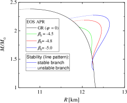
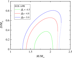
Figure 1: Some properties of NSs in the DEF model with $\alpha_{0}=0$, $\beta_{0}<0$, and using the APR EOS. We show the mass $M$ as a function of the central energy density $\varepsilon_{\rm c}$ (left panel), the mass $M$ as a function of the radius $R$ (middle panel), and the scalar charge $D$ as a function of $M$ (right panel). In all panels, the solid black lines correspond to the GR solutions, which are also solutions in the DEF model. We use different color lines to represent the scalarized branches for $\beta_{0}=-5.0,\,-4.8$, and $-4.5$. NSs past the maximum mass in the $M$-$\varepsilon_{\rm c}$ plane are unstable to radial oscillations. These sequences of stars are shown by the dotted lines.

Recall that the effective potential $V_{\rm eff}$ needs to be sufficiently negative in order to support at least one tachyonic mode [cf. Eqs. (9) and (10)]. For typical NS densities, Eq. (22) implies that scalarization exists for $\beta_{0}\lesssim-4$. Damour and Esposito-Farèse [87] made this estimate using a Newtonian approximation and also confirmed it by integrating the fully relativistic equations of stellar equilibrium. Subsequent works refined the threshold for scalarization to $\beta_{0}\lesssim-4.35$ and also showed that this bound is not very sensitive to the EOS [246, 310, 12]. We note that similar to the GR branch of NSs, in the original DEF model the scalarized solutions are stable up to the maximum mass of the corresponding branch and the stable solutions are generally energetically favorable over the GR NSs. This will be discussed in detail in Sec. III.2.1.

Let us briefly comment on the exact definition of mass in scalar-tensor theories (shown in Fig. 1 and elsewhere). In contrast to GR, the definition of mass in scalar-tensor theories is subtle, due to the fact that these theories violate the strong equivalence principle. This results in the appearance of different possible masses as a measure of the total energy of the star [206, 299, 300, 356, 370]. These works showed that only the so-called “tensor” mass has natural energy-like properties. For example, the tensor mass is positive definite, it decreases monotonically by the emission of GWs and it is well defined even for dynamical spacetimes [206, 299, 300]. In addition, only the tensor mass leads to a physically acceptable picture since it peaks at the same point as the particle number, a property crucial for the stability of the static stars [356, 370]. Therefore, the tensor mass, that is defined as the ADM mass in the Einstein frame, should be taken as the physical mass. As a matter of fact though, for most of the commonly used coupling functions the Jordan frame and the Einstein frame NS masses are identical.

After the discovery of the phenomenon, scalarization was examined for a larger set of parameters and in more detail by Damour and Esposito-Farèse [88]. They showed that the presence of some externally-imposed scalar field background $\varphi_{0}$, as well as considering $\alpha_{0}\neq 0$, smooths the transition to a scalarized state. This is what we described as induced scalarization in Sec. II.3.4. (Strictly speaking, we do not have pure scalarization in this case since GR is not a solution of the field equations anymore). Spontaneous scalarization was further addressed in Salgado et al. [292], which considered the problem in the Jordan frame and performed an approximate Newtonian analysis of the system. They showed that scalarization can be also associated with the fact that the effective gravitational constant in scalar-tensor theories decreases for large scalar fields. It was further argued by Whinnett and Torres [357] that scalarization leads to violation of the weak energy condition in the inner regions of NSs, which can cause instabilities. It was later argued by Salgado et al. [293], that this is not a general feature of scalar-tensor theories and there are subclasses of the theory where the weak energy condition is easily satisfied.

Another consequence of scalarization is that for sufficiently large $\beta_{0}$ the maximum allowed mass for NSs increases compared to GR , which can have various observational consequences. This problem was studied by Sotani and Kokkotas [324] taking into account the effects of various microphysics parameters. Empirical relations were derived for the maximum mass of scalarized NSs that are parametrized with respect to the nuclear saturation parameters and the maximum sound velocity in the core.

Until now we have discussed works that considered negative $\beta_{0}$. However, as we mentioned, when the trace of the energy-momentum tensor is positive, scalarization can also occur for $\beta_{0}>0$ as well, and this scenario introduces qualitative differences relative to our story so far [218]. In particular, for the commonly used coupling function $\alpha(\varphi)=\beta_{0}\varphi$ of theDEF theory, scalarized stars are not stable for very high values of $\beta_{0}$ ($\beta_{0}\gg 1$), which will be further discussed in Sec. III.2.2.

The calculation of NS parameters spanning the DEF theory parameter space provides a challenging technical task. In particular, tests of this theory against binary pulsar observations (described in the next section) require the knowledge of the scalar charges (and its derivatives with respect to the star’s mass) for a large catalog of EOSs. This calculation has been performed most extensively in the works by Anderson and Yunes [14], Guo et al. [148], which provide the results in tabulated form or through surrogate models. Yagi and Stepniczka [365] (see also Horbatsch and Burgess [170]) computed scalar charges in the DEF model analytically by a combination of perturbative weak-field expansion and Padè resummation, and found excellent agreement with numerical calculations.

Spontaneous scalarization for the case of several close-by compact objects was considered in Cardoso et al. [69]. The analytical analysis clearly shows that even though an isolated body might be below the threshold for scalarization, a collection of such bodies can develop a nonzero scalar field while maintaining an average compactness much below the scalarization limit.

We have discussed spontaneous scalarization of NSs so far, but other compact objects can also scalarize. The case of BHs will be considered in Sec. IV, but as an additional nonvacuum example let us briefly discuss the case of boson stars (cf. Liebling and Palenzuela [207] for a review), which were also shown to scalarize [355]. In such systems, one has a complex scalar field as a matter source for the boson star and an additional real scalar field responsible for scalarization similarly to the DEF model. The dynamics of this process was examined by Alcubierre et al. [8] showing that nonlinear development of the scalar field is also observed in the absence of self-interactions in the complex scalar field. Ruiz et al. [288] studied spontaneous and induced scalarization starting with initial data corresponding to stable boson stars in GR. They showed that a strong emission of scalar radiation occurs during the scalarization process.

Observational constraints from binary pulsars:

Up to date the binary pulsars set the best constraints on scalarized NSs in the DEF models [194, 378]. The reason for this lies in the remarkable accuracy of pulsar timing observations. One of the important observables is the shrinking of the orbit of close binary systems due to energy loss caused by GW emission. In contrast to GR, DEF model has an additional scalar degree of freedom that leads to a new channel of energy loss. Thus, the shrinking of the orbit should happen faster. The flux of the scalar dipole radiation, that gives the dominant contribution, is given by [86],

$$F^{\rm dipole}_{\rm scalar}=A\,(1+q_{1}q_{2})^{3}(q_{2}-q_{1})^{2},$$ (32)

where $A$ is a function depending on the properties of the binary, such as its total and reduced mass, and its eccentricity. $q_{2}$ and $q_{1}$ are the scalar charges of each binary component normalized with respect to its mass, $q=D/M$.

Binary pulsar observations were considered in the context of scalarized NSs for the first time by Damour and Esposito-Farèse [88]. They calculated the gravitational form factors (also known as “sensitivities”) of slowly-rotating NSs, that is the set of coupling constants appearing within scalar-tensor theory in the description of the relativistic motion and timing of pulsars, which led to constraint on the $\beta_{0}$ parameter. Only a few such binary systems were known at the time, and $\beta_{0}$ was constrained to be greater than $-5$ using polytropic EOSs. These results were later refined to include realistic EOSs and a limit of $\beta_{0}>-4.5$ was derived in Damour and Esposito-Farèse [90]. In addition, an estimate was made that it would be difficult for LIGO and VIRGO to improve $\beta_{0}$ bounds for most EOS possibilities (some exceptions are pointed out by Sampson et al. [294] and Shao et al. [304]). The reason is that even though the merger events observed by such GW detectors can lead to much stronger scalar dipole radiation, they are inferior in accuracy compared to the radio observations of binary pulsars, leading to weaker overall constraints. The next-generation detectors, though, such as Cosmic Explorer and Einstein Telescope, will be able to improve the bounds on scalar-dipole radiation [294, 304].

An example of how constraints can be imposed on DEF models is presented in Fig. 2, which illustrates how the model fails the double pulsar test for specific values of the theory parameters. In this case, the failure is due to the additional energy loss from scalar GWs predicted by the DEF model, predominantly the dipolar contribution.

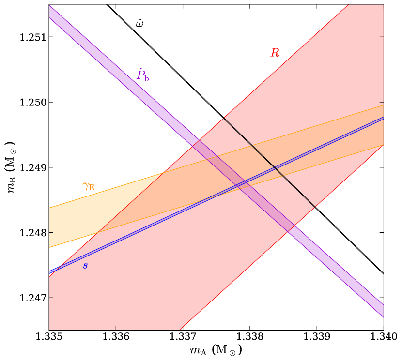
Figure 2: The mass-mass diagram for the double pulsar PSR J0737-3039A/B for the DEF model with $\alpha_{0}=5\times 10^{-4}$, $\beta_{0}=-4$, and assuming the NSs are described by EOS MPA1. Different measured post-Keplerian parameters are shown by the different curves, with the width indicating the measurement uncertainty in each parameter. For the point $\alpha_{0}=5\times 10^{-4}$ and $\beta_{0}=-4$ of the parameter space of the DEF model to be consistent with observations, all curves would have to intersect in a region of the mass-mass plane. This is not the case, as can be seen with the $\dot{\omega}$ (periastron advance) and $\dot{P}_{\rm b}$ (change of orbital period) curves. For further details and for the definitions of the other post-Keplerian parameters see Kramer et al. [194]. Credit: Kramer et al. [194].

With the advances in observational astronomy, more pulsars in binary systems suitable for constraining the scalar dipole radiation have been discovered, a complete and up to date list can be found in Freire [136]. Consequently, observational bounds on the scalar-tensor gravity parameter $\beta_{0}$ for such systems were widely discussed in the literature [129, 22, 137, 305, 354, 304, 350, 194, 75, 378]. The strongest current limit comes from Zhao et al. [378] that practically closes the scalarizaton window for the original DEF model, i.e. the possibility for scalarization is ruled out in this specific case. As we will discuss below, though, there are a number of other well-motivated models where scalarization is still possible, or can not be constrained at all by binary pulsar observations. These include theories with a massive scalar field, Gauss-Bonnet theories of gravity, tensor-multi-scalar theories, or even the standard DEF model when rapid rotation of NSs, which enhances the effect of scalarization, is considered. Furthermore, the theoretical and numerical approaches developed for the study of the DEF model are still applicable to these generalized theories in most situations. Thus, we will spend considerable time on the aspects of the DEF model despite its original form being essentially ruled out.

The constraints on scalarization with $\beta_{0}>0$ using pulsar-timing observations have been investigated in Mendes and Ottoni [221]. Due to the fact that the scalar charge is suppressed as $\beta_{0}$ increases, while the range of masses allowing spontaneous scalarization decreases, it turns out that only weak constraints can be imposed by binary pulsar observations in this part of the parameter space.

Rotating scalarized neutron stars:

So far we have commented only on static NS models. All observed NSs are at least slowly rotating, and some dynamical processes such as NS mergers or stellar core-collapse can produce relatively long-lived rapidly rotating (supramassive) protoneutron stars. Hence, the inclusion of rotation in NS physics is an inseparable part of the goal to explore their astrophysical implications.

Damour and Esposito-Farèse [88] were the first to study slowly rotating scalarized NSs to leading order in rotation frequency, ${\mathcal{O}}(\Omega)$, using the formalism of Hartle [152], Hartle and Thorne [154], which allowed them to calculate the NS moment of inertia (also see Sotani [319]). It is interesting that in this case there is an exact analytical solution for the NS exterior [88]. Static and slowly-rotating NSs for a wide range of realistic EOSs, including examples with hyperons or quark matter, were considered in Altaha Motahar et al. [12]. The extension to second order in the rotational frequency, ${\mathcal{O}}(\Omega^{2})$, was made in Pani and Berti [253], which allowed to calculate rotational corrections to star’s radius and mass, and also its quadrupole moment.

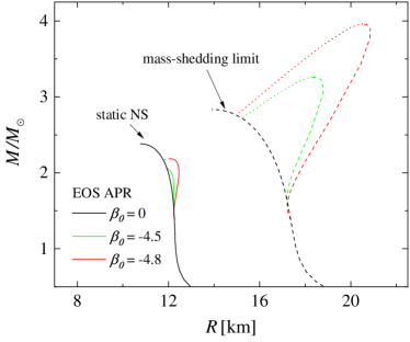
Figure 3: The mass-radius relation for NSs in the DEF-model for $\beta_{0}=0,\,-4.5$ and $-4.8$ and employing the APR EOS. Nonrotating NSs are shown by the solid curves, whereas stars rotating at the mass-shedding limit with the dashed lines. As in Fig. 1, stars unstable to radial oscillations are shown with dotted lines. The radius of rotating stars refers to their equatorial radius.

Rapidly uniformly rotating scalarized stars, without approximation, were obtained by Doneva et al. [121]. They showed that, for a fixed $\beta_{0}$, the maximum deviation from GR that is achieved at the mass-shedding limit is considerably larger compared to the static case, and the range of central energy densities where scalarization is possible is significantly broadened. This can be seen in Fig. 3 where sequences of static scalarized NSs are compared to NSs rotating at the Kepler limit, for the same values of $\beta_{0}$.

There are a number of factors leading to differences with the static case. The first, more intuitive, one is that the rotational energy of the star also acts as a source for the scalar field, and thus can change the onset and degree of scalarization. Meanwhile, the rapidly rotating models tend to be less compact, which can reduce the degree of scalarization. The large deviations from GR compared to the static case, on the other hand, are mainly due to the fact that scalarized stars can sustain much larger angular momentum before reaching the Kepler limit. This is a nonlinear effect that could not be normally caught in the slow rotation approximation.

A natural consequence of the rotation effects above is that the minimum $|\beta_{0}|$ where scalarization is possible changes compared to the static case. Thus, for the same EOS II [100] used by Damour and Esposito-Farèse [88], scalarization happens for $\beta_{0}<-3.9$ in rotating stars [121] compared to $\beta_{0}<-4.35$ in the static case [88]. Therefore, one can conclude that although binary pulsar observations seem to rule-out DEF scalarization for static or slowly-rotating NSs [378], there is still an observationally viable range of $\beta_{0}$ where only rapidly rotating NSs can scalarize. This is potentially relevant for binary mergers and stellar core collapse where such rapidly rotating NSs can form.

A caveat in the previous argument is that, one does not expect the star to rotate uniformly in these extremely dynamical events. Such differential rotation was first studied in Doneva et al. [122], which adopted a simple rotation law that can still capture some of the main properties of the merger remnants, especially a few tens of milliseconds after the merger of the binary [39]. When scalarization is considered, larger values of the maximum mass as well as of the angular momentum can be achieved for supramassive NSs compared to GR. Moreover, the scalar field causes rapidly rotating models to be less quasitoroidal than their general-relativistic counterparts. This can have direct astrophysical implications especially for binary NS mergers where the maximum possible mass and angular momentum of a NS can sustain are crucial to determine the merger outcome and the lifetime of the merger remnant (in case a supramassive or hypermassive NS forms). See e.g., Bauswein et al. [36], Takami et al. [338], Weih et al. [353], Bauswein and Stergioulas [39].

III.1.2 Massive scalar field

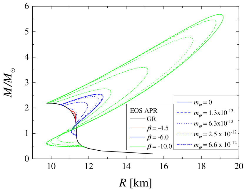
Figure 4: The mass as a function of the radius for EOS APR4. The results for different values of the coupling constant $\beta_{0}$ and mass of the scalar field $\mu$ are plotted. Here the potential is assumed to have the form $V(\varphi)=(\mu^{2}/2)\varphi^{2}$ with a scalar field defined though the action (II.2.3). Credit: Krüger and Doneva [195].

A key property of scalar-tensor theories that was neglected in the studies discussed above is the possibility to have a nonzero scalar field potential. The simplest case is to take a potential that leads to a nonzero scalar field mass $\mu$, but more complicated potentials, such as those with self-interaction terms, can be considered [see Eq. (2)]. Although this seems like a simple extension, it has a dramatic effect on the observational properties of NSs, especially on the GW emission. The reason lies in the different asymptotic behavior of the scalar field. In the case of zero potential the scalar field decreases as $D/r$ at infinity according to Eq. (31). This leads to a nonzero scalar charge $D$ and thus nonzero scalar dipole radiation. In the presence of nonzero scalar field mass $\mu$, though, the scalar field tends exponentially to zero after some characteristic distance related to its Compton wavelength $\lambda_{\varphi}=2\pi/\mu$ as discussed by Ramazanoğlu and Pretorius [273]. Hence, the scalar field is effectively confined to some characteristic radius and its scalar charge is zero. If the orbital separation between the two objects in a binary pulsar system is much larger that $\lambda_{\varphi}$, the dynamics will not be directly altered by the scalar field and there is no significant emission of scalar dipole radiation [10]. Since $\lambda_{\varphi}$ is controlled by $\mu$ in the simplest case of scalar field potential, one can reconcile the DEF-model (for arbitrarily small $\beta_{0}$) with binary pulsar constraints by giving the scalar field a mass $\mu\gg 10^{-16}$ eV.

Scalarized NSs in massive scalar-tensor theories were first studied in the static case [72, 262, 273], and later extended to slow [372] and rapid rotation [111]. The inclusion of a quartic self-interaction term to the potential was considered in Staykov et al. [332]. These works showed that the mass of the scalar field and the self-interaction have similar effects on the scalar field around NSs and they both suppress scalarization. The quartic interaction by itself cannot affect the range of central energy densities where scalarized solutions exist, because it is a nonlinear contribution to the linearized scalar field equation of motion [recall Eq. (11)]. This self-interaction was found to lead to smaller deviations from GR in comparison to the massless case. In contrast, the mass term shrinks the domain of existence of scalarized NSs and for large enough masses no scalarization is possible at all. This is evident in Fig. 4, where NS mass is plotted as a function of its radius for different combinations of $\beta_{0}$ and $\mu$. The massive scalar field solutions are confined between the zero scalar field mass models (the original DEF models) and the GR ones, corresponding loosely speaking to $\mu\rightarrow\infty$. It is interesting that for $\mu\gtrsim 10^{-16}$ eV, the solutions are almost indistinguishable from the massless DEF model. For this reason the latter represents an upper limit on the possible deviations from GR in massive scalar-tensor theories.

The exponential asymptotic behavior of the massive scalar field brings computational challenges to the construction of scalarized NSs, which lead to new numerical approaches [285], which also facilitated the construction of NSs for very negative $\beta_{0}$ and large scalar field masses. Rosca-Mead et al. [285] showed that for sufficiently negative $\beta_{0}$ qualitative changes in the strongly scalarized branch of solutions are possible. For example, the maximum of the scalar field can be located away from the stellar center and in its most extreme form, these solutions are composed of a highly compact NS model surrounded by a scalar field shell. Also, Tuna et al. [347] showed that some scalarized solutions in this part of the $(\beta_{0},\mu)$-parameter space show indications of metastability: they are stable to small perturbations, but have lower binding energy compared to their GR counterparts.

An extension of these results to other forms of coupling functions and scalar field potentials is the asymmetron model [72, 233], which realizes proper cosmic evolution and can account for the cold dark matter. These works studied a massive scalar field together with a conformal factor ${\mathcal{A}}(\infty)>0$ [see Eq. (18)] that suppresses deviations from GR for large scalar fields. Highly negative values of $\beta_{0}$ together with a range of scalar field masses covering several orders of magnitude were explored, including the case when the scalar field Compton wavelength is much smaller compared to the size of the NS. This can significantly affect the stellar structure, but the interplay of $\beta_{0}$, the scalar mass and the form of ${\mathcal{A}}(\varphi)$ can keep the deviations from GR within observational bounds.

III.1.3 Incorporating further physics

New aspects of the original DEF model were recently studied by the inclusion of different physical details. For instance, Silva et al. [310] studied the presence of anisotropic pressure of the nuclear matter both for static and slowly-rotating NSs. The motivation comes from the fact that some theoretical considerations, e.g., with magnetic fields or within the Skyrme model (a low-energy EFT of quantum chromodynamics) [243] suggest that at high densities the NS EOS might have a significant degree of anisotropy [165]. In such a case, the effects of scalarization increase (decrease) when the tangential pressure is bigger (smaller) than the radial pressure. The threshold value of $\beta_{0}$ for the development of scalarization, which in the isotropic case is $\beta_{0}<-4.35$, can be increased due to the presence of anisotropy, thus widening the range of parameters where scalarization is possible.

Another astrophysically interesting extension of scalarization is to include the magnetic fields. According to observations and modeling, NS magnetic field values can span from $10^{8}-10^{12}$ G for standard “old” pulsars, ranging through $10^{16}$ G at the surface of some magnetars, and reaching hypothetically as high as $10^{17}-10^{18}$ G in the cores of newly formed protoneutron stars. Such strong magnetic fields impact the properties of scalarized NSs, including their magnetic deformability, maximum mass, and range of scalarization as studied in Soldateschi et al. [317]. They also found a magnetically-induced spontaneous scalarization, whose essence is the following: strong toroidal magnetic fields can support descalarized configurations, and if the star’s magnetic field decreases during some nonideal magnetohydrodynamical process, the star can undergo a rapid growth of the scalar field, i.e., it scalarizes. The magnetic quadrupolar deformations of scalarized NSs and the related GWs produced by rotating magnetars were studied in Soldateschi et al. [318]

Another interesting extension to the standard DEF model is related to challenging the idea that fundamental physics remains unchanged in the star’s interior, which is a common assumption when constructing a nuclear matter EOS. This was studied in Coates et al. [80] where two models were considered in which the mass of the photon has a different value in the interior and the vicinity of a compact star compared to the mass measured by experiments performed in a weak gravity regime. The first model is based on a Proca-like mass with an effective mass term dependent on $\varphi$. The second model can be thought of as a gravitational Higgs mechanism where the Higgs potential is replaced by the scalar-gravity coupling. In both cases the scalar field undergoes spontaneous scalarization, thus acquiring nonzero value if the compactness passes a certain threshold, providing a mass to the photon by coupling to it in an appropriate manner. Although the focus of Coates et al. [80] is on the electromagnetic field as a proof of principle, these results can be extended to other fields of the Standard Model. The signatures of such a gravitational Higgs mechanism on the behavior of magnetic field of NSs in Einstein-Maxwell theory was studied by Krall et al. [193].

III.2 Dynamics of scalarized neutron stars and binary mergers

The dynamics of isolated NSs can be studied by solving the full nonlinear field equations of scalar-tensor gravity, which is often a challenging task. Instead, one usually first approaches the problem by linearizing the field equations around a background solution, and then analyze the resulting linearized dynamics. The study of nonlinear dynamics is then done when necessary and feasible. We follow this sequence in this subsection. We will then review what happens when NSs is scalar-tensor theories are placed in binary systems.

III.2.1 Linearized dynamics

The studies of the linearized dynamics concern the stability of scalarized stars and the analysis of their quasinormal mode (QNM) spectrum. The latter involves the study of different classes of NS oscillations modes, and which are tied to emission of GWs. See Kokkotas and Schmidt [189] for a review.

Stability:

We have seen that scalarized NSs coexist with their nonscalarized counterparts as solutions the DEF model. Which of these branches of solutions is the one realizable in Nature? One way of answering this question consists in calculating the (fractional) binding energy $M_{0}/M-1$, where $M_{0}$ is the star’s baryonic mass. Through this calculation, Damour and Esposito-Farèse [87] showed that scalarized NSs are usually energetically favorable over the GR ones. We show this in Fig. 5, where we plot the binding energy as a function of the baryonic mass. At constant baryonic mass, the scalarized solutions (solid curve) have larger binding energies relative to the GR solutions (dashed curve), and are then energetically favorable. In addition, we can see a cusp at the maximum of the mass for both for the scalarized and nonscalarized NSs. This suggests that solutions beyond the maximum of the mass (dotted curve in the inset) are unstable.

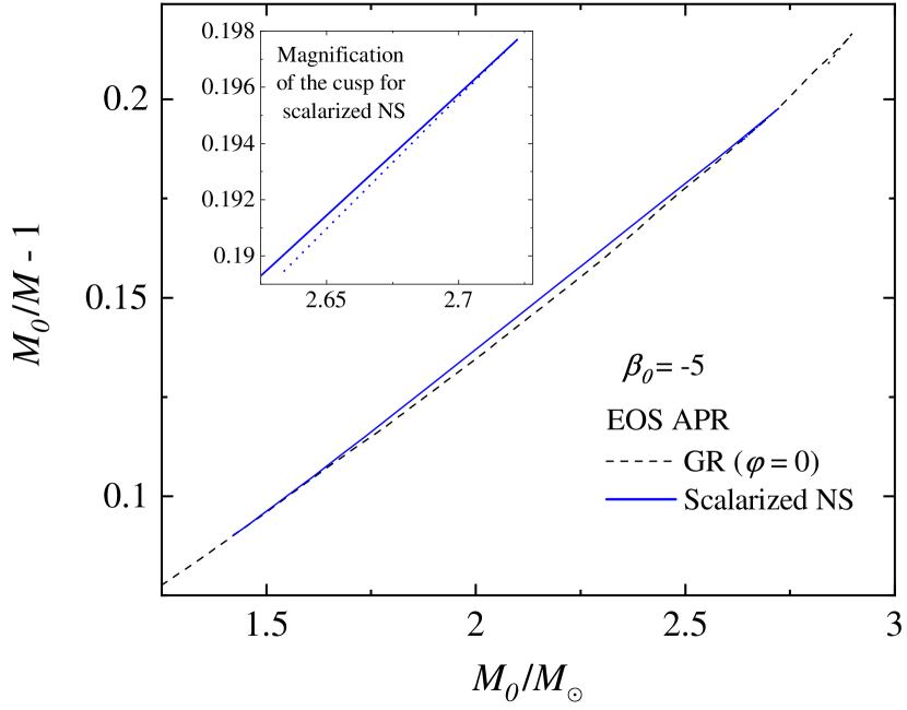
Figure 5: The fractional binding energy $M_{0}/M-1$ as a function of the baryonic mass $M_{0}$ for scalarized NSs in the DEF model with $\beta_{0}=-5$ and using the APR EOS. The inset zooms in the scalarized branch and shows the formation of a cusp at the maximum of the mass.

The stability analysis above relied on the bulk properties of the star. A complementary approach considers the linear perturbations of the star. The first step in this direction was taken by Harada [150], who studied scalar field perturbation in the background of a NS with zero (or constant) scalar field the DEF model. Harada [150] studied the perturbation equations in the frequency domain and showed that the GR solution becomes unstable after a specific critical central energy density. This is the point where the scalarized solution branch out from the GR ones; see Fig. 1. Harada [151] reached similar conclusions, but worked in the context of catastrophe theory. The radial stability of scalarized NSs was also studied by Mendes and Ortiz [220]. They considered metric and scalar field perturbation, and also both signs of $\beta_{0}$. They found that scalarized NSs are stable against linear perturbations and that instability takes place past the point of maximum mass.

Gravitational waves from perturbed NS:

Figure 6: Frequency (left panel) and inverse damping time (middle panel) of the three lowest-frequency radial modes of stellar models in scalar-tensor theories, for coupling function ${\mathcal{A}}(\varphi)=\left[\cosh\left(\sqrt{3}\beta_{0}\varphi\right)\right]^{1/(3\beta_{0})}$ denoted by M1 and ${\mathcal{A}}(\varphi)=e^{\beta_{0}\varphi^{2}/2}$ denoted by M2 with $\beta_{0}=-5$, as functions of compactness. Lines (points) represent values computed with frequency (time) domain techniques. In the figure $F$ stands for the fundamental radial oscillation mode (with no nodes) and $H_{1}$ for its first overtone (with one node), while with $\phi$ is denoted the fundamental scalar mode (with no nodes). The right panel focuses to the details of the fundamental scalar mode, showing its real and imaginary parts. The employed EOS is a two-phase polytrope consisting of a stiff core and a soft crust. Credit: Mendes and Ortiz [220].

Linearized perturbations are also helpful to studying the NS oscillation modes directly related to GW emission. First, let us note that GWs in scalar-tensor gravity can carry additional polarizations compared to GR. In particular, one can have breathing modes in addition to the standard “plus” and “cross” polarizations of GR [359]. Moreover, radial perturbations in scalar-tensor gravity can excite GWs, contrary to what happens in GR. These perturbations source monopole scalar waves, that result in a nonvanishing contribution to the perturbed Jordan-frame Riemann tensor (linearized around a Minkowski background) in the transverse-traceless gauge [86, 247]. For DEF-like scalar-tensor theories this requires $\alpha_{0}\neq 0$. This contribution is then linked to existence of a breathing polarization mode of the GW. We can then conclude that radially oscillating scalarized NSs in a scalar-tensor theories with $\alpha_{0}\neq 0$ will emit GWs with amplitude controlled by $\alpha_{0}$.

The first study of radial oscillations of NSs in the DEF model was performed in Sotani [320] in the Cowling approximation [83, 217]. In this approximation, the spacetime is held fixed while only the fluid and the scalar field are perturbed. Despite its limitations, the Cowling approximation allows one to study the influence of the scalar field on the fluid’s radial oscillation frequencies and the total energy radiated by scalar waves. The full problem, i.e., when both the metric and the scalar field perturbations are taken into account, was addressed by Mendes and Ortiz [220]. This work found a new family of modes, which were named scalar modes, that have no counterpart in GR. The results show that they have quite distinct frequencies and damping times compared to the fluid radial oscillation modes. In Fig. 6 we show the frequencies and damping times of the fundamental fluid radial oscillation mode and its first overtone, as well as the fundamental scalar radial mode, as functions of the stellar compactness. We see in the right panel of the figure that scalarized NSs become unstable at the maximum mass and it is the scalar mode which is responsible for the instability. This contrasts with GR where it is the fundamental radial fluid mode that becomes unstable at the maximum of the mass.

Not only the radial oscillations of scalarized NSs will differ significantly from the GR case, but the nonradial modes, that are related to the tensorial gravitational wave emission, can be strongly influenced by the scalar field. The behavior of nonradial oscillations modes, which are sources of the usual tensor polarizations of GWs, can also be strongly affected by the scalar field. These perturbations can be classified as “polar” or “axial”, depending on how they behave under parity transformations [275, 346].

In particular, scalar field perturbations are of the polar type, meaning that they only couple to polar perturbations of the fluid and metric. In GR, these perturbations are the most efficient GWs sources. Sotani and Kokkotas [322] were the first to study the nonradial oscillations of scalarized NSs. They used the Cowling approximation, in which only polar-parity fluid perturbations are dynamical. This simplifies the problem considerably and Sotani and Kokkotas [322] calculated the (fundamental) $f$- and the (pressure) $p$-modes frequencies. In a follow-up work, Sotani and Kokkotas [323] went beyond the Cowling approximation and derived equations, for both axial and polar perturbations, that included metric perturbations. They analyzed only the simpler axial perturbations (discussed below). A study of the polar perturbations only became possible after new techniques were developed in GR by Krüger and Kokkotas [197, 196]. These techniques were then used in scalar-tensor theory by Krüger and Doneva [195], who also considered self-interacting massive scalar fields. Krüger and Doneva [195] found that the scalar field leaves very “clear” imprints on the oscillation frequencies of NSs. The extension of these results for rapidly-rotating NSs, but now back to the Cowling approximation, was made by Yazadjiev et al. [371]. They also studied in details the Chandrasekhar-Friedman-Schutz instability driven by rotation [71, 138].

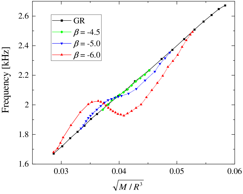
Figure 7: The $f$-mode frequency (for $\ell=2$) as a function of the average NS density $\sqrt{M/R^{3}}$ for several values of $\beta$. The SLy EOS is used [124]. Credit: Krüger and Doneva [195].

An interesting property of NSs oscillations in GR, is the almost linear and EOS-independent relation between the quadrupole ($\ell=2$) $f$-mode frequency and the average density of the NS [16]. Sotani and Kokkotas [322] and Krüger and Doneva [195] showed that this linear scaling is dramatically broken by scalarization. We show this in Fig. 7, where we also see that the deviations from GR increase with the increase of $|\beta_{0}|$.

Another class of modes that can be loosely speaking attributed to the “oscillations” of the spacetime itself are the axial spacetime $w$-modes. These modes are somehow easier to calculate (without approximations) because in this case the perturbations of the fluid and the scalar field are zero. The axial modes of scalarized NSs were considered for the first time in Sotani and Kokkotas [323], who the frequencies and the damping times of different classes of $w$-modes were calculated. The extension of these results to a variety of realistic EOSs including nuclear, hyperonic and hybrid matter, was done by Altaha Motahar et al. [13], while the case of massive self-interacting scalar fields was studied by Altaha Motahar et al. [11]. The effect of scalarization in stronger on the damping times compared to the frequencies, and, in general, their values are reduced compared to GR. In addition, EOS-independent relations between $w$-mode properties known to exist in GR can also be obtained in scalar-tensor theory.

A class of NS modes related to the crustal torsional oscillation was studied in Silva et al. [313] for the DEF model in the Cowling approximation. These oscillations most probably follow the giant flares in soft gamma-ray repeaters [176, 336, 337] and are associated to motions in the NS crust. Silva et al. [313] found that for values of $\beta_{0}$ consistent with binary pulsar constraints, the effect of scalarization on the torsional oscillation frequencies is smaller than the uncertainties in the microphysics modeling of the crust.

III.2.2 Nonlinear stability and collapse to a black hole

While the stability and the oscillations of a scalarized NS can be studied perturbatively, the formation of the scalar hair starting from a GR NS solution is a full nonlinear process. More precisely, the initial exponential growth of the scalar field, starting from unstable GR solution, can be modelled by linearized dynamics, but the subsequent saturation of the scalar field to an equilibrium value is a nonlinear phenomenon.

The transition from a nonscalarized to a scalarized NS was first considered by Novak [245] (also see Degollado et al. [97]), who studied the nonlinear evolution in spherical symmetry. The numerical simulations of Novak [245] showed that the scalar field for an unstable GR NS first grows exponentially, and then saturates, with the system saturating to an equilibrium scalarized endstate. A consequence of the work by Novak [245] was the proof of nonlinear stability of scalarized NSs. That is, the numerical simulations showed that the scalarized NSs have stable evolution if the full nonlinear system of field equations (in spherical symmetry) is considered. Although not strictly dedicated to the stability analysis, fully nonlinear evolution of scalarized NSs were performed in a series of papers that we discuss later. This provides strong support for the stability of these objects under the most general circumstances.

Novak [246] studied the collapse of a scalarized NS to a BH in spherical symmetry. Since BH no-hair theorems include DEF models (see e.g., Herdeiro and Radu [161] for a review), the resulting BH will be bald and the scalar field has to be radiated away during collapse. This takes places in the form of scalar waves, similarly to what we discussed in the case of radial NS oscillations in Sec. III.2.1.

Our discussion so far covered the case $\beta_{0}<0$ case. Palenzuela and Liebling [252] and Mendes and Ortiz [219] studied the end state of the tachyonic instability in scalar-tensor theories for representative coupling functions with $\beta_{0}>0$ and realistic EOSs. This was done both through an energy balance analysis of the existing equilibrium configurations, and by nonlinear dynamical simulations. They found (contrary to the $\beta_{0}<0$ case) that the final state of the instability is highly sensitive to the details of the coupling function, varying from gravitational collapse to spontaneous scalarization. They also found that in the original DEF model (remember, $\alpha(\varphi)=\beta_{0}\varphi$) that scalarized solutions can become unstable compared to the GR ones when $\beta_{0}\gg 1$. However, stability can be recovered for all values of $\beta_{0}$, by considering different coupling functions. This is the case for coupling functions with bounded values, such as $\alpha(\varphi\to\infty)=\alpha_{\infty}$ for some constant $\alpha_{\infty}$. This distinction could give rise to novel astrophysical tests for determining the detailed form of the coupling.

III.2.3 Stellar core-collapse

Once we know that equilibrium scalarized NS solutions exist in the DEF model and they are stable against linear perturbations, the next step is to study how they are formed. Isolated NSs can form after the collapse of the core of a massive star during a supernova explosion. A NS on the other hand can collapse to a BH if a threshold for the mass and the angular momentum is reached. All these are highly dynamical nonlinear processes that can have strong observational signatures both in the electromagnetic and the GW signals.

The first study of a degenerate stellar core collapse (more specifically with white dwarf initial data) to a scalarized NS through a bounce and the formation of a shock was done by Novak and Ibanez [247]. The simulations were done in spherical symmetry, which allowed them to calculate only the resulting gravitational monopolar radiation. They found that the emitted breathing modes can be potentially detected by LIGO or VIRGO. More interestingly, the emitted signal will be substantially different than the collapse of a NS to a BH, allowing one to distinguish between them.

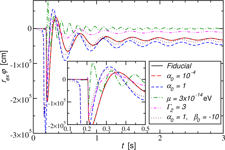
Figure 8: The scalar wave $r\varphi$ during stellar core-collapse extracted at $5\times 10^{4}\,{\rm km}$. The legend lists deviations from the fiducial parameters $\mu=10^{-14}\,{\rm eV},\leavevmode\nobreak\ \alpha_{0}=10^{-2},\leavevmode\nobreak\ \beta_{0}=-20,\leavevmode\nobreak\ \Gamma_{1}=1.3,\leavevmode\nobreak\ \Gamma_{2}=2.5,\leavevmode\nobreak\ \Gamma_{\rm th}=1.35$, where $\mu$ is the scalar field mass, and $\Gamma_{1}$, $\Gamma_{2}$ and $\Gamma_{\rm th}$ are parameters of the polytropic EOS and the thermal contribution. See Sperhake et al. [328] for more details. Credit: Sperhake et al. [328].

Gerosa et al. [146] studied the problem of spherically symmetric core collapse in the DEF model in further details. Two types of initial data were used: collapse of a stellar iron core and collapse of “realistic” NS progenitors that were obtained from computations of stellar evolution. Depending on the theory parameters three possible outcomes of the core collapse are possible – collapse to a GR NS, collapse to a scalarized NSs, collapse to a short-lived protoneutron star followed by a (nonscalarized) BH formation. It was in the latter case that the most prominent GW signal with a clear signature from the presence of nontrivial scalar fields was observed. While the fluid dynamics during the collapse is only weakly affected by the scalar field, the contrary is not true – the scalar radiation depends strongly on the specifics of the matter collapse as well as on the choice of the coupling parameters $\alpha_{0}$ and $\beta_{0}$.

The inclusion of a scalar field mass to the core collapse simulations has some interesting consequences [328]. The waveform $r\varphi$ during such events is shown in Fig. 8. The mass itself does not have a large influence on the dynamics, but it allows to reconcile the theory with binary pulsar observations for a much larger range of $\alpha_{0}$ and $\beta_{0}$, as discussed in Sec. III.1.2. Thus, a dramatic increases in the radiated GW signal observable even with the existing LVK detectors was predicted. A prominent feature is that we expect to receive an inverse chirp signal from such events that will last for years, with a near monochromatic signature on time scales of $\sim 1$ month. The extension of these results to the case of self-interacting scalar field potential was made by Cheong and Li [73] and Rosca-Mead et al. [284]. Constraints on the theory based on the scalar field evolution in the Einstein frame were imposed by Geng et al. [144]. The problem was considered in greater detail in Rosca-Mead et al. [286] where the three possible scenarios of the collapse outcome in scalar-tensor theory with sufficiently negative $\beta_{0}$ were found. These constitute the formation of a BH following multiple NS stages, the multi-stage formation of a strongly scalarized NS, and the single-stage formation of a strongly scalarized NS. Rosca-Mead et al. [284] found that the resulting GW signal can reach a signal-to-noise ratio of over $20$ for the existing GW detectors, which has the potential to put strong constraints on the theory.

III.2.4 Dynamical scalarization and neutron star mergers

Another highly dynamical and nonlinear process that has important astrophysical, and especially GW implications is the binary NS mergers. This problem can be more challenging to solve compared to the stellar core-collapse because it is not possible by construction to apply certain approximations, such as spherical symmetry. That is why the binary merger dynamics in the DEF model was addressed only years later, first by Barausse et al. [33] and Shibata et al. [305]. The overall conclusions of both works are similar and they reside in the fact that even if one or both of the NSs are not scalarized before the merger, they can develop nonzero scalar fields during the inspiral. This was called dynamical scalarization. The main advances in Shibata et al. [305] constitute in using several realistic EOS with consistently derived bounds on the parameter $\beta_{0}$ as well as developing an initial data solver for scalarized binary NSs. The overall results demonstrated the significant change of the inspiral GW signal at the moment of dynamical scalarization and afterwards. The reason is that the inspiral is accelerated due to the scalar dipole radiation and the total number of GW cycles is significantly decreased with respect to the general relativistic case.

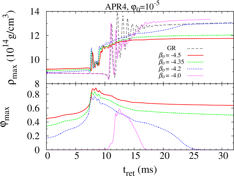
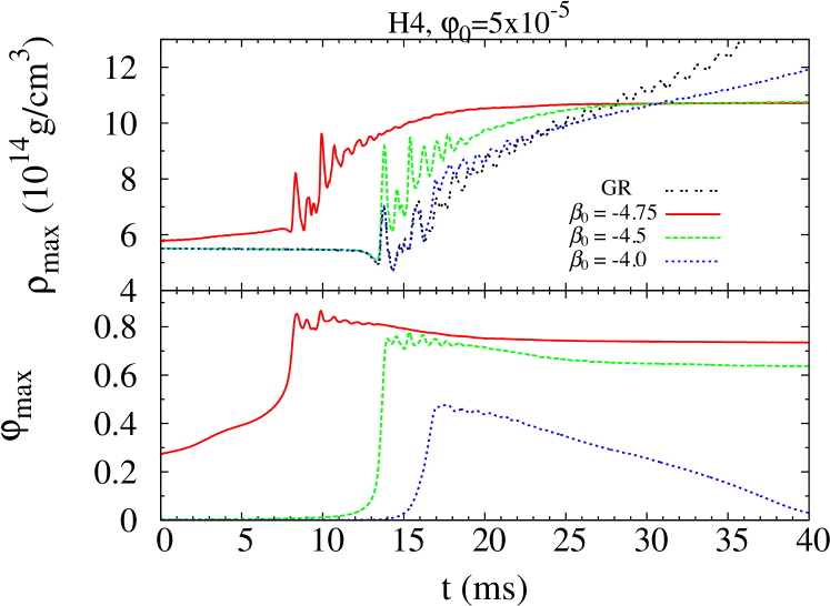
Figure 9: Evolution of the maximum values of the rest-mass density $\rho_{\rm max}$ and scalar field $\varphi_{\rm max}$ during NS merger for several models with total mass $M=2.7\leavevmode\nobreak\ {\rm M}_{\odot}$ with the APR4 EOS (top panel) and the H4 EOS (bottom panel). The merger sets in at the time as the maximum density steeply increases. We note that for $\beta_{0}\geq-4.2$ with APR4 EOS and for $\beta_{0}=-4.75$ with H4 EOS, the scalarization already occurred at $t=0$. Credit: Shibata et al. [305].

The actual merger and the post-merger phase were addressed only in Shibata et al. [305] which showed that dynamical scalarization can happen not only after the inspiral, but also during the merger since a very massive compact star is formed in this process. The evolution during NS merger of the maximum values of the rest-mass density $\rho_{\rm max}$ and scalar field $\varphi_{\rm max}$ for several binary NSs with total mass $M=2.7\leavevmode\nobreak\ {\rm M}_{\odot}$ and several values of $\beta_{0}$ is shown in Fig. 9. Two EOSs are considered in the two panels and the cosmological value of the scalar field is taken to be $\varphi_{0}=10^{-5}$. Some of the binary NSs are not scalarized at the beginning of the evolution (the models with $\varphi_{\rm max}=0$ at the beginning), but the values of $\beta_{0}$ are chosen such that all of them develop scalar fields at a certain point of the evolution. The actual merger of the two NSs is marked by the rapid increase of $\varphi_{\rm max}$. Afterwards, either a hyper- or supramassive NS is formed, or the merger remnant collapses to a bald BH and the scalar field is radiated away. In agreement with the studies of equilibrium differentially rotating NSs discussed in Sec. III.1.1, the scalarized merger remnant can sustain a larger mass without collapsing to a BH [122]. This is evident in the right panel of Fig. 9 where collapse to a BH is observed in pure GR, while a supramassive NS is formed after the merger scalar-tensor gravity for small enough $\beta_{0}$.

The quasiperiodic oscillations of the merger remnant were examined by Shibata et al. [305] showing a clear distinction compared to the GR case. Such oscillations were studied in a series of papers in GR (see e.g. Bauswein and Janka [37], Bauswein et al. [38], Hotokezaka et al. [172], Bauswein et al. [40], Takami et al. [338], Clark et al. [77], Takami et al. [339], Rezzolla and Takami [276], Maione et al. [213]) mainly as a tool to determine the nuclear matter EOS from the post-merger GW signal. The observed differences with the scalarized case can potentially be used to discriminate between GR and modified gravity theories. This is specially the case, because scalarized merger remnants are produced only if specific initial conditions, related to the mass of the merging compact objects and the specifics of the EOS, are met [305].

Taniguchi et al. [342] took a different approach, where quasi-equilibrium sequences of binary NSs at different time instants were calculated instead of performing time evolution. This approach is well known in GR [147, 340, 341], and it is assumed that the characteristic time of the system to settle to an equilibrium is much smaller than the inspiral time scale. This is supposed to give a relatively accurate picture of the binary evolution even close to the merger. The results are in agreement with Shibata et al. [305], while the small deviations relative to Barausse et al. [33] are probably due to the fact that GR initial data were used in the latter. Taniguchi et al. [342] showed that the absolute value of the binary binding energy is smaller than in GR. In addition, the GW cycles prior to the merger were significantly reduced compared to pure GR once scalarization kicks in, and the effect is considerably stronger compared to the one due to tidal interactions.

The post-Newtonian (PN) approximation has also been a valued tool to model NS inspiral in the DEF model. Initial work has focused in tensor-multi-scalar theories and simple scalar-tensor theories that do not allow scalarization [86, 89, 232, 203]. This approach cannot be immediately applied to the case dynamical scalarization since this is nonperturbative effect absent in the weak field regime. Palenzuela et al. [251] was the first to address this issue. They used the equations of motion at 2.5PN order, derived in scalar-tensor gravity of Mirshekari and Will [232], and supplemented them with a “Newtonian feedback” mechanism to account scalarization in the inspiral. The resulting inspiral evolution was found to be in agreement with the numerical simulations of Barausse et al. [33]. The approach of Palenzuela et al. [251] is computationally inexpensive, and this allowed them the study large portions of the parameter space, including (un)equal-mass and eccentric binaries. This approach can also be used to efficiently generate inspiral GW templates in the DEF model. A further step forwards was taken by Sennett and Buonanno [302], that introduced a methodology called post-Dickean expansion. Their main improvements with respect to Palenzuela et al. [251] is a 1PN extension of the feedback mechanism. The post-Dickean expansion was compared against the quasi-equilibrium calculations of Taniguchi et al. [342], and it was shown that it can accurately predict the onset and magnitude of dynamical scalarization.

Sennett et al. [303] took a different approach in the perturbative study of the inspiral, that consisted of an analytic model of dynamical scalarization using an effective action. The motivation was to cure two deficiencies in the previous PN studies. In effective action approach, the nonlinear scalarization process is reduced to a pair of cubic equations that have a closed-form solution depending on the binary separation when dynamical scalarization happens and on the magnitude of the developed scalar charge. This simplifies the problem relative to Palenzuela et al. [251] and Sennett and Buonanno [302]. In addition, the effective action approach allows one to construct a simple two-body Hamiltonian, that can be used to compute the binary’s binding energy. Sennett et al. [303] used this stablished dynamical scalarization as a second-order phase transition. Khalil et al. [185] extended these results to general theories admitting scalarization, either for BHs or NSs, and are valid for adiabatic (quasistationary) and quasicircular orbits. Khalil et al. [184] took a step further, where these approximations were dropped and the dynamical evolution around the phase transition to the scalarized regime was studied. The results showed that in some cases, assuming a quasistationary evolution might not be accurate enough even for quasicircular binaries.

At last, Ponce et al. [261] studied the effect of the scalar field on the electromagnetic radiation emitted in the merger of magnetized NSs. They found that deviations in the emitted electromagnetic flux due to scalarization are not negligible yet challenging to measure. However, if combined with GW observations, constraints on scalar-tensor theory can, in principle, be placed, showing the usefulness of multi-messenger astronomy.

III.3 Astrophysical implications of scalarized NSs in the DEF model

In this subsection we will discuss in greater detail the astrophysical implications of scalarized NSs. Many aspects have already been covered in the previous sections, such as the binary pulsar observations, NS oscillations, stellar core-collapse, and binary mergers, as they naturally appeared in the presentation. Here, we will shed further light on possible astrophysical implications of scalarization, trying to be as complete as possible under two main parts. First, we will discuss the astrophysical implications directly related to electromagnetic observables. Afterwards, we will address the problem of universal relations for scalarized NS models.

Electromagnetic observations:

Scalarized NSs in the DEF model and its extensions were studied in a variety of astrophysical scenarios in attempt to probe the existence of the scalar field. Since NSs are often times surrounded by accretion disks, it is natural to study the effect of a nontrivial scalar field on disk’ properties. The simplest model is called “thin disk”, where particles are assumed to move on geodesics around the central compact object. Any small perturbation acting upon these particles will lead to oscillations around their equilibrium orbit with some characteristic (epicyclic) frequencies. Epicyclic and orbital frequencies are thought be, in one way or another, related to the interpretation of different accretion disk properties. An example are the quasiperiodic oscillations (QPOs) observed in the spectrum of low-mass x-ray binaries. For this reason, some works calculated these frequencies in the spacetime of scalarized NSs. DeDeo and Psaltis [95] did this for nonrotating NSs, Staykov et al. [330] included slow-rotation and also a mass to the scalar field, while Doneva et al. [123] studied rapidly-rotating NSs. The conclusion of these works is that if one takes into account current observational constraints, only the cases of rapid rotation and massive scalar fields leave room for significant effect of the scalar field. Yet, a question that deserves further works is how one can disentangle uncertainties in the NS EOS and in the disk model from modifications to GR.

Another promising observational property of accretion disks around a compact objects is the shape of the Fe $K_{\alpha}$ fluorescent line at 6.4 keV. This line is expected to be observed in greater details with future x-ray mission such as ATHENA. Bucciantini and Soldateschi [65] argued that both the intensity of the low-energy tails and the position of the high-energy edge of the line change due GR modification are potentially observable in the future.

Accretion onto NSs can also trigger a process called “gravitational phase transition”, named in analogy with matter phase transitions from confined nuclear matter to deconfined quark matter [200]. This process can happen when the maximum mass of the scalarized NSs is smaller than the maximum mass of the zero scalar field (GR) solution. The idea is then that if a scalarized NS close to this maximum mass accretes some matter it may pass beyond the stability point. In GR this would cause a collapse to a BH. In scalar-tensor theory, the star will radiate its scalar hair and evolve towards the zero scalar field (i.e., GR) branch. A significant amount of GWs can be produced in this process, potentially detectable with the next generation of GW detectors.

The NS surface as an emitter of x-ray radiation is also an important probe in strong-field gravity, because the electromagnetic radiation is emitted from a region with large spacetime curvature. In this regard, the simplest observable is the gravitational redshift of surface atomic lines. The redshift carries information about the NSs mass, radius, spin, and in scalar-tensor gravity, about the scalar field. DeDeo and Psaltis [94] showed that scalarization has significant effect on the redshift, but only for negative enough values of $\beta_{0}$. Such values are already ruled out by binary pulsar observations. One could entertain the idea that a small scalar field masses could allow for large deviations in the redshift relative to GR, while reconciling the theory with with binary-pulsar constraints [262, 273, 111]. A study of this problem has not been performed yet.

The emission of x-ray pulse profiles emitted by hot spots at NS surfaces have also received considerable attention recently. Observations of these signals allow for a relatively clean inference of NS masses and radii [352]. This potential was met with observations [55, 224, 281] by the Neutron Star Interior Composition Explorer (NICER) [28]. Sotani [321] and Silva and Yunes [316] developed pulse-profile models for NSs in massless DEF model. Xu et al. [362] considered the case of massive scalar fields and Hu et al. [173] studied the positive $\beta_{0}$ case. Silva and Yunes [315] made the first study of what constraints can be placed on the DEF model with pulse-profile observations and found they can be competitive with binary pulsar observations. However, this work is rather simple and not at the level of realism found in analysis of real data. This remains an important avenue for future work.

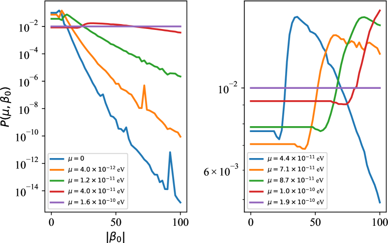
Figure 10: The posterior probability density for $\beta_{0}\in[-100,\ 0]$ for various assumed values of the scalar field mass $\mu$ in the massive version of the DEF model introduced by Ramazanoğlu and Pretorius [273] (marginalized over various EOS). One can obtain the bound $\beta_{0}\gtrsim-20$ for $\mu\lesssim 2\times 10^{-11}$ eV (left panel), but there is no effective bound for higher masses, at least in the interval $\beta_{0}\in[-100,\ 0]$ (right panel). No bound is possible for $\mu\gtrsim 10^{-10}$ eV using this data, since scalarization does not occur for such high $\mu$ values within the considered $\beta_{0}$ interval. Credit: Tuna et al. [347].

At last, Tuna et al. [347] used the NS mass and radius measurements [250, 54] to constrain the massive extensions of the DEF model. They obtained a weak lower bound $\beta_{0}\gtrsim-20$ for scalar field masses $\mu\lesssim 2\,\times 10^{-11}$ eV; see Fig. 10. This is significant since no other bound is known for $\mu\gg 10^{-16}$ eV. These results show that large scalar masses enable agreement with observations, even for extremely negative $\beta_{0}$, and demonstrate the difficulty to constrain scalarization when the scalar field is massive.

Universal relations:

One of the biggest obstacles in using NS observations to test modified theories of gravity is the uncertainty in the NS EOS, which remains unknown at high-densities [204, 41]. In general, modifications to NS properties predicted by different EOSs are degenerate with changes to the underlying gravity theory used to model these stars. One way to break this degeneracy is to consider relations between different NS properties that depend weakly on the EOS [368, 107]. In fact, in Sec. III.2.1, we had already met one such example relating the QNMs’ frequencies and damping times and the mean density of NSs. Here we will focus on other EOS-independent relations connecting various equilibrium properties of scalarized NSs.

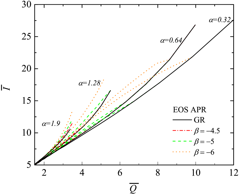
Figure 11: Comparison between ${\bar{I}}-{\bar{Q}}$ relations for GR and scalar-tensor theory, for several values of $\beta_{0}$, where ${\bar{I}}=I/M^{3}$ and ${\bar{Q}}=QM/J^{2}$. The presented data are only for APR EOS in order to have better visibility, but the deviations for other EOS are very small, typically below roughly $2\%$. Sequences for different values of the normalized rotational parameter $\alpha=M\Omega/2\pi$ are given, where $\Omega$ is the angular velocity of the star. Credit: Doneva et al. [120].

A class of universal relations that attracted considerable attention is the I-Love-Q relations, connecting the normalized moment of inertia, tidal Love number and quadrupole moment of NSs [366, 367]. If any two quantities in the I-Love-Q trio are measured independently, one can constrain deviations from GR by checking whether these observations agree with the GR I-Love-Q relation within the observational accuracy. Silva et al. [309] applied this strategy to constrain dynamical Chern-Simons gravity [177, 9] using observational data from LVK and NICER. The application to scalarization models has not been done yet.

The I-Love-Q relations for scalarized NSs were studied in slow [253] and rapid [120] rotation, including the case of massive scalar fields [173, 111]. In Fig. 11 we show the relation between the normalized moment of inertia $\bar{I}$ and quadrupole moment $\bar{Q}$ for sequences of scalarized NSs with fixed rotational parameter $\alpha=M\Omega/2\pi$ is given in. We see that for small absolute values of $\beta$, e.g., $\beta_{0}=-4.5$, the deviations from GR are practically negligible for slow rotation (e.g., $\alpha=0.32$) while they are enhanced by rapid rotation. As we already saw, massive scalar fields allow much smaller values $\beta_{0}$, while remaining consistent with observations. Hence, these scalarization models allow for larger differences between the scalarized NS universal relations and the GR ones [111].

The moment of inertia $I$ and the quadrupole moment $Q$ are among the leading order multipole moments in the asymptotic expansion of the metric functions at infinity. There are infinitely many other higher order multipole moments, though, and it is interesting to explore whether similar universal relations hold for them. This was first addressed in GR [256, 363] where such universal relations were derived for the higher multipole moments when proper normalization is applied. Pappas and Sotiriou [258] and Pappas et al. [257] extended these results to scalarized NSs. This required the generalization of the multipole moment formalism of Geroch [145], Hansen [149] to scalar-tensor gravity. Pappas et al. [257] showed that future observations of QPOs of low-mass x-ray binaries can, in principle, be used can be measure different NS properties and tell apart different gravity.

Another class of universal relations studied in the context of the DEF model connects the NS moment of inertia and compactness. This is motivated by Lattimer and Schutz [205] (see also Breu and Rezzolla [59]), that used this relation to argue that pulsar timing observations could lead to a measurement of the moment of inertia to within $10\%$. These relations were generalized to scalarized NSs with massless scalar field potential by Altaha Motahar et al. [12], and later to massive self-interacting scalar fields by Popchev et al. [263]. Similar to the I-Love-Q relations, only the massive scalar field case leads to large deviations from GR when observational constraints are taken into account.

Ofengeim [248] proposed to connect the physical parameters of static NSs, such as mass, radius, central energy density, pressure, and sound speed, at the maximum-mass point for a given EOS. This is based on the observations that the nuclear matter EOS (without phase transitions) can be well parameterized by only two parameters [211]. As a result, Ofengeim [248] derived multiple constraints on the nuclear matter EOS. Danchev and Doneva [93] generalized these relations to scalarized NSs. They showed how sensitive these relations can to the underlying theory of gravity. Thus, all the EOS restrictions derived in GR should be taken with care, since the possibility for GR modifications are rarely taken into account when interpreting observational data.

III.4 Extended scalar-tensor theories beyond the Damour-Esposito-Farèse model

Until now we discussed scalarization in the DEF model or other DEF-inspired models. However, s we saw in Sec. II.2, spontaneous scalarization is also possible for other modified theories of gravity. Here, we will discuss such theories where scalarized NS solutions were obtained.

Scalar-tensor theories with disformal coupling

Minamitsuji and Silva [230] studied NS scalarization in scalar-tensor theories with disformal coupling of the form (17). More specifically, instead of the standard conformal transformation between Einstein frame metric ($g_{\mu\nu}$) and Jordan frame metric (${\tilde{g}}_{\mu\nu}$)

$$g_{\mu\nu}={\cal A}^{2}(\varphi){\tilde{g}}_{\mu\nu},$$ (33)

where ${\mathcal{A}}(\varphi)$ is a function of the scalar field related to the Jordan frame coupling between the scalar field and the Ricci scalar, we have a more general and complicated transformation that also involves scalar field derivatives:

$$g_{\mu\nu}=A^{2}(\varphi)\left[{\tilde{g}}_{\mu\nu}+\Lambda B^{2}(\varphi)\nabla_{\mu}\varphi\nabla_{\nu}\varphi\right],$$ (34)

where $B(\varphi)$ is a function of the scalar field and $\Lambda$ is a parameter of dimensions of [length]². The motivation behind this modification of the conformal factor comes from Bekenstein [42] that aimed to find the most general coupling constructed from the metric $g_{\mu\nu}$ and the scalar field $\varphi$ that respected causality and the WEP. More recently, Andreou et al. [17] showed that such disformal coupling is actually equivalent to a kinetic coupling with the Ricci scalar and thus is contained in the minimal action (II.2.1) (see Sec. II.2.1 for a detailed discussion).

Minamitsuji and Silva [230] showed that for negative values of the disformal coupling parameter $\Lambda$, scalarization can be suppressed, while for large positive values of $\Lambda$ stellar models cannot be obtained. This study also explored the universal relations between the moment of inertia and the compactness of NSs, and they determined the range of parameters where these relations can deviate significantly from GR.

Scalar-Gauss-Bonnet theory:

Another well-studied modified gravity theory that allows for NS scalarization is scalar-Gauss-Bonnet gravity discussed in Sec. II.2. Interestingly, spacetime curvature itself as well as matter can be the source of the scalar field in this theory. Scalarized NS solutions in scalar-Gauss-Bonnet gravity were studied for the first time in Doneva and Yazadjiev [112], Silva et al. [312]. They exhibit quite different features compared to the DEF model while being qualitatively similar to NS solutions in other classes of Gauss-Bonnet theories where scalarization is not possible [254, 186, 289]. For example, for a given central energy density the stellar mass is always smaller compared to GR. Moreover, normally there is only one bifurcation point at small central energy densities and afterwards the branches of solutions are terminated because of violation of the regularity conditions.

In Fig. 12, we show the branches of scalarized NS solutions for a coupling function $f(\varphi)=-\lambda^{2}(2\beta)^{-1}[1-\exp(-\beta\varphi^{2}/4)]$. Here, $\lambda$ is a parameter with dimensions of [length]^-1 that controls the coupling strength in the action (II.2.3). Note that the sign of $f(\varphi)$ is opposite to the one discussed in Sec. II.2.3 and thus can not lead to BH spontaneous scalarization since in vacuum $\mu_{{\rm eff}}^{2}>0$ as defined in (27). However, due to the presence of matter NSs can scalarize. Scalarized NS solutions were found also for the more “conventional” sign of $f(\varphi)$, namely $f(\varphi)=\lambda^{2}(2\beta)^{-1}[1-\exp(-\beta\varphi^{2}/4)]$ [112].

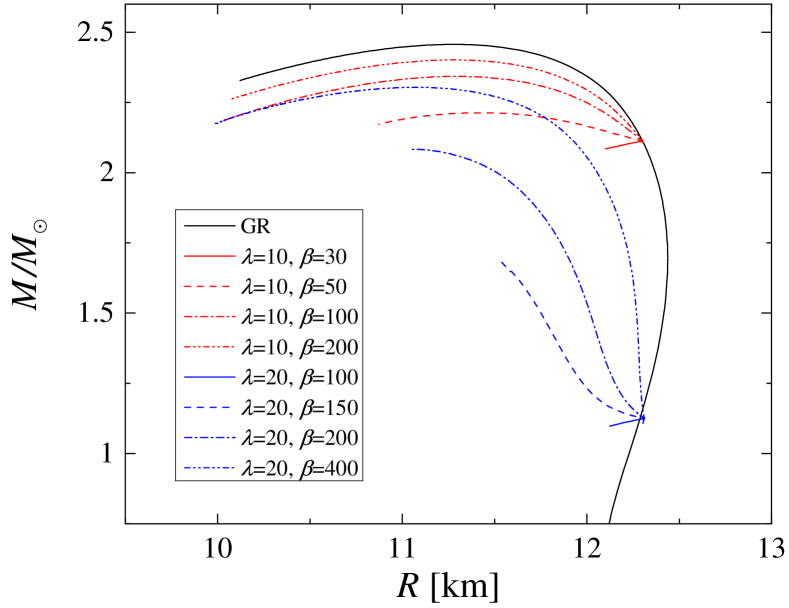
Figure 12: Scalarized NSs in scalar-Gauss-Bonnet gravity. We show the mass as a function of the radius for GR (trivial branch with $\varphi=0$) as well as several scalarized branches with different values of the scalar field coupling parameters $\lambda$ and $\beta$. Credit: Doneva and Yazadjiev [112].

Little is currently known about the astrophysical implications of these stars. Kuan et al. [198] considered the spherically symmetric core collapse of a non-compact star either to a protoneutron star or to a BH in Gauss-Bonnet theory. They also proposed a realistic physical mechanism for the formation of isolated scalarized BHs and NSs The complexity of the problem is greatly increased with respect to GR, though, and there are fundamental difficulties such as the loss of hyperbolicity of the evolution equations for certain ranges of parameters, effectively limiting the maximum possible scalar field to relatively low values (see also East and Ripley [125, 126], Ripley and Pretorius [283] for the case of BHs). Core-collapse simulations show that the remnant in scalar-Gauss-Bonnet theory can be very rich with (de)scalarization happening at intermediate or final stages of the collapse depending on the properties of the progenitor and the theory parameters. Since breathing modes are absent in this theory, the effect on GW emission can be estimated only if one drops the assumption of spherical symmetry. This is something that has not been done yet in any modified gravity theory due to problem’s complexity.

The Ricci-Gauss-Bonnet model:

One can further modify the action in scalar-Gauss-Bonnet gravity to include additional terms. This is the case of Ricci-Gauss-Bonnet model discussed in Sec. II.2.4. This model has interesting advantages such as the possibility to reconcile scalarization with cosmology. Here we will focus on the NS solutions this theory that were considered by Ventagli et al. [348]. This work made thorough exploration of the theory parameter space in order to find the sectors where NS solutions exist. Since their scalar charge is nonzero, in these sectors one can put severe constraints on the theory based on the binary pulsar observations, similar to the DEF model (see Sec. III.1.1).

The free parameters in the theory, as evident from the action (II.2.4), are $\beta$ and $\alpha$ that control the coupling strength to the Ricci scalar and the Gauss-Bonnet invariant respectively. In Fig. 13 the existence of NS solutions is shown in a two-dimensional plot spanning the parameters $\alpha$ and $\beta$ in a broad range, for a fixed central energy density and the MPA1 EOS [237]. The white area corresponds to the region of the parameter space where the GR solution is stable against scalar perturbations. Throughout the parameter space that is spanned by $\alpha$ and $\beta$, a new unstable mode appears every time one crosses a black line. These unstable modes can be labeled by the number of scalar field nodes (denoted by $n=0,1,2,3$ in the figure). Any point in the parameter space that lies within some grey region corresponds to a configuration where the GR neutron star solution is unstable. The red (respectively blue) area corresponds to the region where scalarized solutions with $n=0$ (respectively $n=1$) nodes exist.

As one can see, scalarized solutions exist in only part of the parameter space. In the $\beta>0$ and small $\alpha$ range (in white in the figure) the GR neutron starts are stable. This is exactly the region most interesting from the point of view of BH scalarization and connection to cosmology Antoniou et al. [24, 25], see also Sec. IV.1.2. Thus, including a Ricci coupling to the scalar-Gauss-Bonnet action seems to allow for BH scalarization while evading the binary pulsar constraints.

Fig. 13 is only for one EOS and a specific central energy density. Different EOSs and central densities can lead to significant deformations of the existence and stability regions. The general point made in Ventagli et al. [348], though, is that a stability (white) region always survives.

Figure 13: Regions of existence of scalarized solutions in the $(\alpha,\beta)$ plane for the MPA1 EOS with central energy density $\varepsilon_{c}=6.3\times 10^{17}\leavevmode\nobreak\ \text{kg}/\text{m}^{3}$. In GR, a star with this choice of $\varepsilon_{c}$ and EOS is light, with $M_{\text{GR}}=1.12\leavevmode\nobreak\ {\rm M}_{\odot}$. The red (respectively blue) region is the region where scalarized solutions with $0$ (respectively $1$) scalar field node exist. The grey contours obtained by Ventagli et al. [349] are superimposed, which represent the lines beyond which GR solutions with the same density are unstable to scalar perturbations with $0,1,2,$ etc nodes. We see that the region where there exist scalarized solutions with $n$ nodes is included in the region where the GR solutions are unstable to scalar perturbations with $n$ nodes, but much smaller. The dashed boundary for the blue region corresponds to a breakdown of the integration inside the star. Credit: Ventagli et al. [348].

Tensor-multi-scalar theories:

Another class of gravity theories where NS scalarization was considered, is the tensor-multiscalar theories [86], whose basics we discussed in Sec. II.2. In this theory the gravitational interaction is mediated by the spacetime metric $g_{\mu\nu}$ and $N$ scalar fields $\varphi^{a}$ which take values in a coordinate patch of an $N$-dimensional Riemannian (target) manifold ${\cal E}_{N}$ with a positive definite metric $\gamma_{ab}(\varphi)$ defined on it [86, 169].

The main features of tensor-multiscalar theories is the inclusion of more than one scalar field and a structure called the target space metric. In that sense, there are two directions to go in order to obtain scalarized NSs. The first one is to consider a mixture of several, more or less equivalent, scalar fields that was the approach in Horbatsch et al. [169]. There, the authors examined the case of two scalar fields in the form of a complex scalar with a maximally symmetric target space metric $\gamma_{ab}$. Doneva and Yazadjiev [114] studied scalarization in tensor-multi-scalar gravity in a more complicated setup, namely when $\gamma_{ab}$ is a three-dimensional maximally symmetric space together with a nontrivial map $\varphi:$ spacetime $\rightarrow$ target space. While the solutions in Horbatsch et al. [169] can be viewed as generalization of the DEF model to multiple scalar fields, the scalarized NSs in Doneva and Yazadjiev [114] have some quite distinct properties and they can be considered more as a limiting case of the topological NSs discovered by Doneva and Yazadjiev [115]. More specifically, the scalar field is zero in the stellar center, while only its first derivative is zero in the DEF model. The scalar charge for the scalarized stars in tensor-multi-scalar theories is zero as well. This automatically reconciles this theory with the binary pulsar observations (due to the absence of scalar dipole radiation), while still allowing for large deviations from GR. Another interesting property is the fact that there is non-uniqueness of the scalarized solutions with respect to the central energy density – something that was never observed before at least for scalarized NSs. Fig. 14 illustrates this property. Interestingly, Kuan et al. [199] showed that all these solutions are stable until the maximum NS mass regardless of the non-uniqueness.

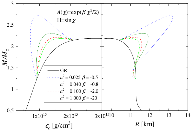
Figure 14: Tensor-multi-scalar theories: the mass as a function of the central energy density (left panel) and as a function of the stellar radius (right panel) for scalarized NSs in tensor-multi-scalar theories where the target space metric represents a three-dimensional maximally symmetric space and we have a nontrivial map $\varphi:$ spacetime $\rightarrow$ target space. Sequences of scalarized solutions for different combinations of parameters are given. Observe the appearance of non-uniqueness of the solutions with nonzero scalar field for certain combinations of the parameters (e.g., the small central energy density region for the blue dotted line). Credit: Doneva and Yazadjiev [114].

Other scalarization models:

Apart from models of scalarized NSs already discussed, other works have attempted to consider scalarization in other more exotic theories of gravity or even different types of scalarization.

For example, Azri and Nasri [30] considered NS scalarization in what is called scalar-connection gravity, where gravity is mediated by a scalar field and the connection. Other types of scalarization in standard scalar-tensor theories, but if we allow for different scalar field potentials. Minamitsuji and Tsujikawa [231] showed this by considering the potential $V(\varphi)=m_{\phi}^{2}f_{B}^{2}[1+\cos(\phi/f_{B})]$ of a pseudo-Nambu-Goldstone boson. Here $(\mu_{\phi}$, $f_{B})$ are constants with dimensions of length and the scalar field has negative mass, $\mu^{2}=-m_{\phi}^{2}$. Minamitsuji and Tsujikawa [231] showed that in this case the scalar field sits at its vacuum expectation value far away from the source, while inside a NS, a symmetry restoration can take place resulting in a new type of scalarization. This theory also has the advantage that it avoids cosmological instabilities present in some other scalarization models.

IV Black hole scalarization

In this section, we discuss spontaneous scalarization of BHs in three parts. First, in Sec. IV.1 we consider models in which BHs can scalarize in vacuum due to couplings between scalar field and curvature scalars. Next, in Sec. IV.2 we discuss models in which scalarization is induced by the presence of extra fields (e.g., gauge or matter fields) in the BH spacetime. Finally, in Sec. IV.3 we review a selection of other models of BH scalarization.

IV.1 Black hole scalarization: vacuum spacetimes

As we saw in Sec. II, some gravity theories admit the same vacuum BH solutions as GR, and yet can give rise to new branches of solutions, with scalar hair, once certain conditions are met. The prototypical example is described by scalar-Gauss-Bonnet theories, whose action, in the absence of matter, is given by Eq. (II.2.3), namely,

$$S =\frac{1}{16\pi G}\int{\rm d}^{4}x\,\sqrt{-g}\,\left[R-2g^{\mu\nu}\partial_{\nu}\varphi\partial_{\mu}\varphi+f(\varphi)\mathscr{G}\right].$$

As we discussed in Sec. I, the first models exhibiting BH scalarization in vacuum were proposed in Doneva and Yazadjiev [113] and Silva et al. [312]. These models remain to date the most studied BH scalarization models in the literature and for this reason, they will be our main focus in this section.

As explained in Sec. II.2.3, in theories described by the action (II.2.3), a no-hair theorem guarantees that the BH solutions of GR are unique to the theory, as long as $({\rm d}^{2}f/{\rm d}\varphi^{2})_{\varphi=\varphi_{0}}\mathscr{G}<0$, for some constant $\varphi_{0}$ [312]. If this condition is violated, scalar field perturbations can become tachyonic unstable and the endpoint in expected to be a nonlinear, scalarized BH [283]. Scalarized BHs have been shown to form dynamically, as outcomes from the core collapse of an initially unscalarized star [198].

In what follows, we first review our understanding of isolated scalarized BHs in scalar-Gauss-Bonnet theories, focusing on their properties and their stability. We then review what is understood about when they are found in binaries. Finally, we give an overview of vacuum BH solutions in models that generalize the action (II.2.3).

IV.1.1 Spherically symmetric and rotating scalarized black holes

Spontaneously scalarized BH solutions were first found in Doneva and Yazadjiev [113], Silva et al. [312]. What distinguishes these works is the choice of the coupling function $f(\varphi)$ that couples the scalar field to the Gauss-Bonnet invariant [cf. Eq. (II.2.3)], respectively,

$$f =(\lambda^{2}/12)\,[1-\varepsilon\exp(-6\varphi^{2})],$$ (35a)

$$f =(\eta/8)\,\varepsilon\,\varphi^{2},$$ (35b)

where $\lambda^{2}$ and $\eta$ are coupling constants with dimensions of [length]² and $\varepsilon=\pm 1$, which should not to be confused with the energy density of Sec. III. Both coupling functions agree in the small-$\varphi$ limit (i.e., when $\varphi\ll 1$) and therefore make the same prediction for the onset of scalarization of GR BHs. This threshold can be found by searching for bound state solutions, i.e., time-independent solutions of the linearized field equation for $\varphi$ around a GR BH, which are regular at the event horizon $r_{\rm h}$ and that vanish at spatial infinity. Hence, the determination of the scalarization threshold reduces to a boundary value problem. In the simplest case of a Schwarzschild BH of mass $M$, the dimensionless quantity $\eta/M^{2}$ plays the role of the eigenvalue and can be determined numerically with standard techniques, such as the shooting method. The smallest eigenvalue gives the threshold for the formation of the “fundamental” scalarized BH solution (in the sense that the radial profiles of the scalar field has $n=0$ nodes). The other eigenvalues give the thresholds for the formation of “excited states”, that is, solutions with one or more nodes. In Fig. 15 we show the results of such a calculation in the spacetime of a Schwarzschild BH and $\varepsilon=1$, as done in Silva et al. [312]. We remark that no bound states can form for $\varepsilon=-1$, because the effective mass of scalar field perturbations is positive and therefore the effective potential is positive definite. See the discussion in Sec. II.1.2.

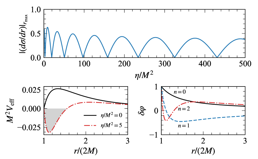
Figure 15: Results of the numerical integration of the equation of a monopole ($\ell=m=0$) scalar perturbation $\delta\varphi$ on a Schwarzschild BH background. Top panel: the asymptotic value of $|{\rm d}\sigma/{\rm d}r|$ (with $\sigma\equiv r\,\delta\varphi$), evaluated at a point $r_{\rm max}\gg r_{\rm h}$, far away from the event horizon $r_{\rm h}=2M$, as a function of $\eta/M^{2}$. Cusps mark when bound state solutions form. They signal the transition between stable Schwarzschild BHs and scalarized solutions. Bottom-left panel: effective potential $V_{\rm eff}$ (see Sec. II.1.2) for $(\eta/M)^{2}=0$ and $5$. In the latter case, $V_{\rm eff}$ develops a negative region and can support bound states. Bottom-right panel: radial profiles of $\delta\varphi$ for the first three bound states, corresponding to $\eta/M^{2}=2.902$, $19.50$ and $50.93$. These profiles have $0$, $1$ and $2$ nodes, respectively. The properties of these solutions are shared between the models of Doneva and Yazadjiev [113], Silva et al. [312]. Credit: Silva et al. [312].

While both models (35) agree in their prediction of the threshold for scalarization, they differ significantly in their prediction of the properties of the nonlinear, scalarized solution, as already discussed in Sec. II.1. In Fig. 16 we show the branches of scalarized BHs, in a parameter space spanned by the dimensionless scalar charge and BH mass. The solutions were obtained by solving the full system of field equations (see e.g. Julié et al. [180] for detailed discussion). The results are for the Gaussian coupling (35a) with $\varepsilon=1$. We show the fundamental, zero-node scalar field solution (dashed, red curves) and also the excited scalarized BHs (solid, green and blue curves). We see that the branches of excited BHs can terminate at finite masses $M$. This is due to a violation of an inequality at the BH horizon which must be satisfied for the scalar field to be real-valued and is typical of scalar-Gauss-Bonnet theories; see e.g., Kanti et al. [182] and Antoniou et al. [23]. The parameters in the coupling function (35a) are chosen in such a way that this disappearance of BH solutions does not affect the fundamental branch. For other couplings, such as Eq. (35b), even this branch can violate the regularity condition shortly after bifurcation [see e.g., Doneva et al. [106], Silva et al. [311]]. Hence, the domain of existence of scalarized solutions in the Gaussian model (35a) is larger with respect to that of the “quadratic” model (35b).

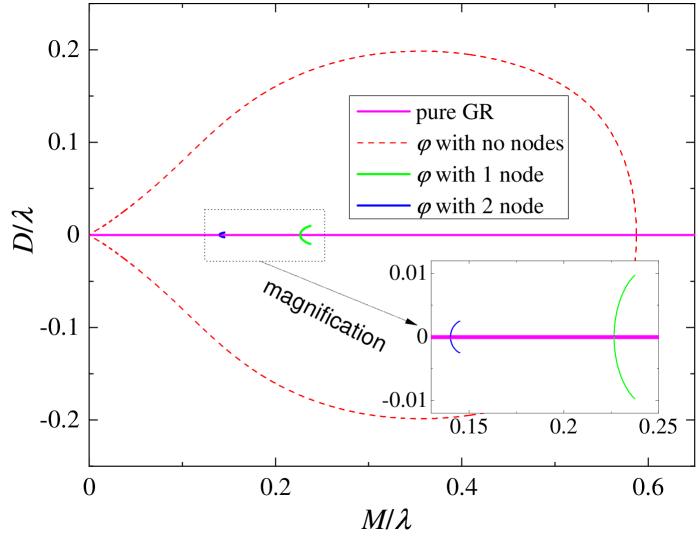
Figure 16: The scalar charge $D$ normalized to the coupling parameter $\lambda$ as a function of the normalized BH mass $M/\lambda$ for sequences of scalarized BH solutions. The branches with different colors corresponds to solutions with different number of scalar field nodes, where only the nodeless scalar field solutions can be stable [49]. The GR solutions have zero scalar field and thus zero $D$, and that is why they lie on the $x$-axis, depicted in magenta. The scalarized branches are symmetric with respect to the $y$-axis due to the reflection symmetry ($\varphi\to-\varphi$) in the theory. Figure adopted from Doneva and Yazadjiev [113].

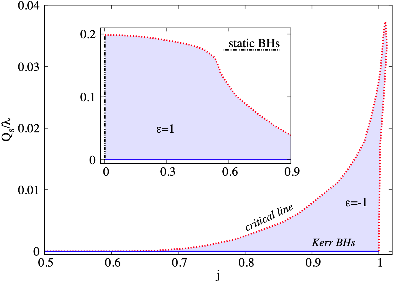
Figure 17: Rotating scalarized BHs in the Gaussian model (35a). The shaded regions represent the domain of existence of scalarized rotating BHs in the plane spanned by the dimensionless scalar charge ($Q_{\rm s}/\lambda$) and spin ($j=a/M$). These regions are bound by the Kerr family of solutions $Q_{\rm s}/\lambda=0$ (solid blue line) and, in the nonrotating limit, by the Schwarzschild solution (black dot-dashed line), and also when the regularity condition for the scalar field is violated (dotted curve). The inset shows the case for positive coupling constant studied in Cunha et al. [84], while the main panel shows nonlinear spin-induced scalarized BHs. Credit: Herdeiro et al. [164].

Asymptotically flat, spinning scalarized BHs in the Gaussian models (with $\varepsilon=1$) and quadratic theories were explored respectively by Cunha et al. [84] and Collodel et al. [82]. In discussing these solutions, it is convenient to consider a plane spanned by the dimensionless scalar charge $Q_{s}/\lambda$ and dimensionless spin parameter $j\equiv J/M^{2}$, where $J$ is the angular momentum of the BH. Figure 17 shows the domain of existence of scalarized rotating BH solutions. In particular, focus on the inset which corresponds to $\varepsilon=1$ in Eq. (35a). We see that as the spin increases, so does the existence domain (shaded region) of the solutions. This result can be understood in terms of the Gauss-Bonnet invariant not being positive-definite for the Kerr metric [74]. More specifically, a Kerr BH develops increasingly larger regions where the Gauss-Bonnet invariant is negative as the spin increases and hence suppressing scalarization. As a consequence, the deviations relative to GR predictions on physical observables (e.g., the location of the innermost stable circular orbit (ISCO) of massive particles or the BH shadow) are smaller for rapidly rotating BHs. See Fig. 18 for an example. Collodel et al. [82] studied the quadratic coupling (35b) and reached similar conclusions. They also obtained radially excited solutions (i.e., scalar field profiles with nodes in the radial direction) and also the existence of “angularly” excited rotating BHs (i.e., scalar field profiles with nodes in the angular directions).

Figure 18: Gravitational lensing and shadow produced by rotating BHs under similar observation conditions. The left panel corresponds to a scalarized BH with mass $M/\lambda\approx 0.237$ and spin $j=0.24$. The right panel corresponds to a comparable Kerr BH. Credit: Cunha et al. [84].

IV.1.2 The stability of scalarizated black holes and implications to model building

Having established the existence of scalarized BHs, the natural next task is to study their stability. A first indication comes from the study of the thermodynamical properties of such BHs. Doneva and Yazadjiev [113] found that the scalarized solutions belonging to the fundamental branch in the Gaussian model are thermodynamically favored relative to the Kerr solution (35a), in the sense that they have a smaller Wald entropy [351]. This suggest the stability of the former, i.e., in a dynamical process BHs in this model would evolve towards a state of smaller entropy. In contrast, in the quadratic coupling (35b) model always results in scalarized BHs with higher entropy relative to their GR counterparts. These observations remain true in the case of rotating BHs [164, 82].

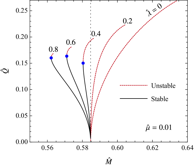
Figure 19: Scalar-charge-mass diagram for scalarized BHs with a quadratic scalar-Gauss-Bonnet model with a scalar field potential $V(\varphi)=(\mu^{2}/2)\varphi^{2}+(\lambda/2)\varphi^{4}$. The figure uses dimensionless quantities obtained by factors of $\eta^{1/2}$: BH charge $\hat{Q}=Q/\eta^{1/2}$ and mass $\hat{M}/\eta^{1/2}$, and scalar field parameters $\hat{\mu}=\mu\eta^{1/2}$ and $\hat{\lambda}=\lambda\eta^{1/2}$. The vertical line marks the threshold for scalarization $\hat{M}_{\rm th}$. BHs with $\hat{M}\geqslant\hat{M}_{\rm th}$ are radially unstable, while the Schwarzschild solution is stable. For large $\hat{\lambda}$, we can obtain solutions with $\hat{M}<\hat{M}_{\rm th}$ and form two branches. The ones which are radially unstable solutions are denoted with a dashed line (upper branch) and those stable to radial perturbations are denoted with a solid line (lower branch). The dot marks are the solutions marginally stable, which correspond to a minimum mass, but maximally scalar charged BH for fixed $\hat{\mu}$ and $\hat{\lambda}$. Credit: Macedo et al. [212].

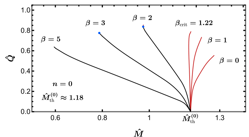
Figure 20: Similar to Fig. 19, but now in “mixed” model, where a quadratic coupling between scalar field and Ricci tensor is added to the quadratic scalar-Gauss-Bonnet interaction. In this figure, similar to Fig. 19, we show the charge $\hat{Q}=Q/\alpha^{1/2}$ and mass $\hat{M}/\alpha^{1/2}$ made dimensionless by division by $\alpha^{1/2}$, for different values of scalar-Ricci coupling $\beta$. See Eq. (II.2.4) for the theory’s action. The black lines correspond to values of $\beta$ for which all scalarized BHs have masses below the GR instability mass threshold, while the red lines mark values of $\beta$ that lead to scalarized BH masses that are larger than the GR mass threshold. Past the turning points (marked with blue dots), the BHs are expected to be unstable to radial perturbations. Credit: Antoniou et al. [25].

A complementary question is whether scalarized BHs are stable to linear perturbations. The first step in this direction was carried by Blázquez-Salcedo et al. [49] which considered radial scalar field and metric perturbations. They showed that Schwarzschild BHs become unstable at the scalarization threshold and that the stability of the fundamental (i.e., the zero-node) scalarized solution depends on which model in Eq. (35) is considered: in the quadratic case all solutions are unstable, whereas stable solutions exist in the Gaussian model.

This important difference between the two models can be traced back to the higher-than-quadratic terms in the scalar field in the theory’s action. More concretely, Silva et al. [311] and Minamitsuji and Ikeda [228] showed the inclusion of a quartic-interaction, say $(\zeta/16)\,\varphi^{4}\,{\mathscr{G}}$, is sufficient to yield stable BH solutions, as long as, $\zeta$ is negative and satisfies $\zeta/\eta<-0.8$. These two conditions are satisfied by the Gaussian model. Indeed, expanding Eq. (35a) to order ${\cal O}(\varphi^{4})$, we find $\zeta/\eta=-3/2$, helping explain the stability of BHs in this model.

It was later shown by Macedo et al. [212] that the original quadratic model can be made stable under radial perturbations by making the scalar field massive and self-interacting $V(\varphi)\propto\mu^{2}\varphi^{2}+\lambda\varphi^{4}$, as discussed in Fig. 19. From an EFT perspective, these terms are of lower order compared to the quartic scalar-Gauss-Bonnet interaction and hence should be included. A similar analysis was also performed for the Ricci-Gauss-Bonnet model by Antoniou et al. [25] and is show in Fig. 20. See also Doneva et al. [108] for a study of scalarization with massive scalar fields.

The nonlinear stability of BHs in this model have also been studied in the time domain by Ripley and Pretorius [283]. They found evidence for regions in mass-coupling parameter space in which the end state of the radial instability of the Schwarzschild BH is a stable scalarized BH. For larger couplings however, regions where the time-evolution equations change character from hyperbolic to elliptic appear outside the BH horizon. This signals a regime in which the theory does not have a well-posed initial-value problem. (See Hilditch [166], Ripley [282] for discussions.) These results are in agreement with earlier findings by Blázquez-Salcedo et al. [49], but in the linear regime. The radial stability of scalarized BHs in the Ricci-Gauss-Bonnet model introduced in Sec. II.2.4, was analyzed by Antoniou et al. [26]. They found that although the Ricci scalar does not affect the scalarization threshold, it can, at the nonlinear level, stabilize the BHs in the quadratic model.

The problem of nonradial perturbations of scalarized BH solutions, which is relevant in the context of testing such theories with ringdown GW signals, was addressed in a series of papers by Blázquez-Salcedo and collaborators [47, 48]. On the other hand, the stability of rotating scalarized BHs remain as an open problem, even in the slow rotating limit.

IV.1.3 Spin-induced scalarization

One property of the Gauss-Bonnet invariant of the Schwarzschild metric is that it is positive definite everywhere and, as a consequence, spontaneous scalarization can only occur for positive values of the coupling constant. Does this always have to be the case? In the case of the Kerr metric, it is known that regions where $\mathscr{G}<0$ outside the outer horizon are possible if the BH spins with $a/M\geqslant 0.5$ [74] suggesting the possibility of a spin-induced scalarization when the coupling constant is negative, i.e., $\varepsilon=-1$ in Eqs. (35).

Although conceptually simple, the problem is not straightforward to analyse because (i) the analytic form of $\mathscr{G}$ forbids the separation of variables as done in Sec. I and thus the determination of the scalarization threshold, in principle, will require more sophisticated numerical methods compared to the Schwarzschild case and (ii) the Kerr metric (with $a/M\geqslant 0.5$) has regions where $\mathscr{G}$ can be either negative or positive, where in the latter regions, for negative coupling constants, the effective mass may trigger a superradiant instability [64]. To overcome these difficulties, Dima et al. [101] reduced the $(2+1)$-dimensional nonseparable scalar field equation into a $(1+1)$-dimensional system of equations which are coupled through spherical harmonic multipole indices $l$ and $m$. They then performed time-domain numerical integration of the scalar field borrowing methods previously developed to study superradiant instability [103]. Dima et al. [101] showed that the tachyonic instability is the dominant one and charted the parameter space in which spin-induced scalarization would occur. This is shown in Fig. 21. Hod [167] worked analytically in the infinitely-large coupling limit ($\eta/M^{2}\to\infty$) and confirmed the expectation that $a/M\gtrsim 0.5$ is the minimal necessary spin value for which spin-induced scalarization occurs. The corrections for large, but finite, coupling were obtained by Hod [168].

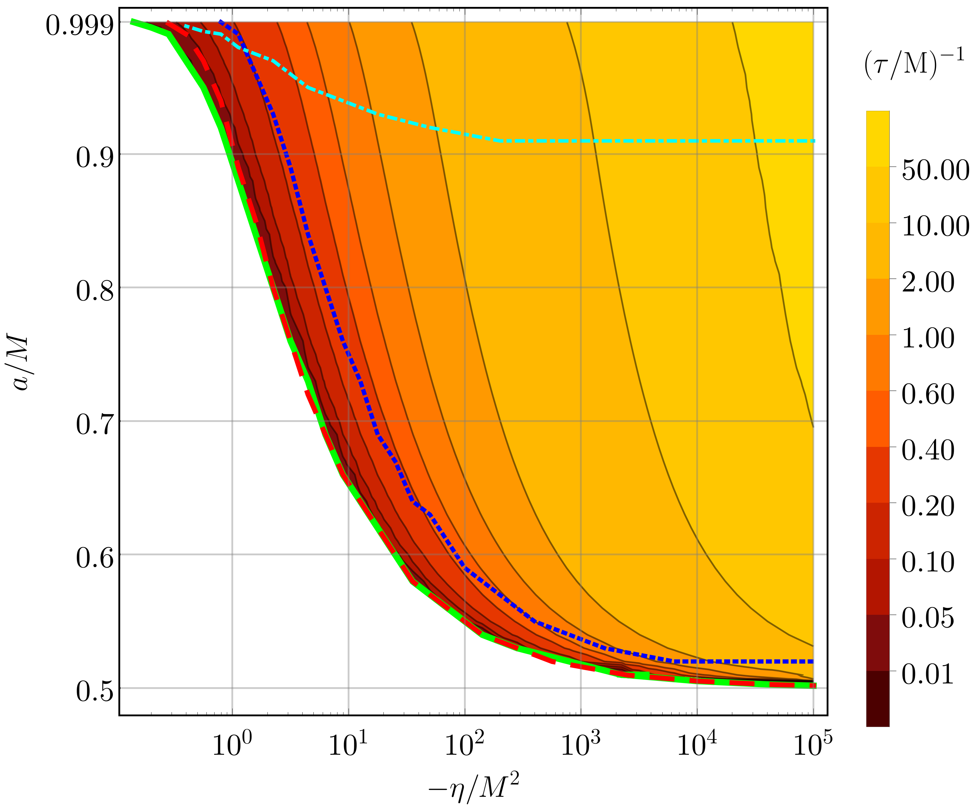
Figure 21: Instability timescale $\tau$ for spin-induced scalarization in the dimensionless spin $a/M$ and dimensionless coupling constant $-\eta/M^{2}$ plane. The instability threshold for the total reconstructed field is shown by the solid green line, while the threshold when the $m=0$ modes are excluded is shown by a blue dotted line. The red dashed line corresponds to the instability threshold for the $m=0$ odd modes, while the dot-dashed cyan line marks the instability threshold for the spherical mode $l=m=0$. Credit: Dima et al. [101].

Nonlinear spin-induced scalarized BH solutions were obtained by Herdeiro et al. [164] and by Berti et al. [44]. They confirmed the existence of scalarized BHs solutions in the parameter space region in which linear theory predict the spin-induced tachyonic instability. In Fig. 17 we show the domain of the spin-induced scalarized BHs in the Gaussian model (35a). We see that scalarized solutions only exist for $j\gtrsim 0.5$, and that their scalar charge increases with spin. Moreover, there are solutions that can violate the Kerr bound $j\leq 1$ on BH spins.

A complementary approach to that of Dima et al. [101], was used by Doneva et al. [104], Doneva and Yazadjiev [116]. In these works the scalar field equation is evolved in (2+1)-dimensions, i.e., without doing a multipolar decomposition. The influence of a non-vanishing scalar field mass explored in Doneva et al. [105]. A similar time-domain study, but using the hyperboloidal foliation method [376], was performed by Zhang et al. [377] and a model with both the Pontryagin and Gauss-Bonnet invariants was studied by Myung and Zou [242]. Annulli et al. [19] studied the effect of strong magnetic fields on spin-induced scalarization. They found that the magnetic field suppresses this effect, i.e., it pushes the scalarization threshold to larger values of the dimensionless spin $j$ of the BH.

The case of spin-induced scalarization has been much less studied in terms on its stability and on how additional nonlinear interactions affect the scalar charge.

IV.1.4 Scalarized black holes in binary systems

Most work in BH scalarization has focused on isolated BHs, but to be able to confront these models against GW observations one has to turn to the two-body problem. What phenomenology would we expect in BH binaries? To answer this question we will first consider works that explored the nonlinear regime of the late inspiral and merger of BH binaries, a regime that relies on numerical relativity. Next, we will consider works that focus on the inspiral alone, a regime which can be modeled with PN theory.

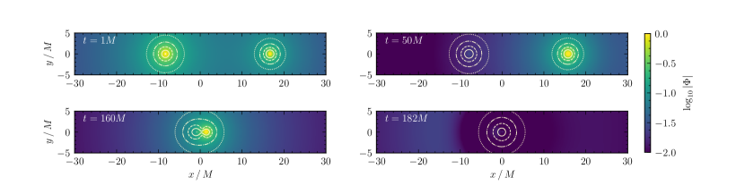
Figure 22: Dynamical descalarization in binary BH head on collisions. Scalar field and Gauss–Bonnet dynamics on the $xy$–plane of the BHs with initial mass-ratio $q=m_{1}/m_{2}=1/2$. We show the amplitude of $\log_{10}|\Phi|$ (color map) together with the isocurvature levels of the Gauss–Bonnet invariant at the beginning of the evolution (top left), during the BHs’ approach (top right), shortly before the collision (bottom left) and shortly after the merger (bottom right). These levels correspond to $1M^{-4}$ (solid line), $10^{-1}M^{-4}$ (dashed line), $10^{-2}M^{-4}$ (dot-dashed line) and $10^{-3}M^{-4}$ (dotted line). Credit: Silva et al. [314].

The first study in this direction was done by Silva et al. [314], which studied the scalar field dynamics (i.e., in the decoupling limit) in head-on collisions and nonspinning, quasicircular inspirals of binary BH spacetimes obtained from numerical relativity simulations. This work adapted the methods developed in Witek et al. [360] for shift-symmetric scalar-Gauss-Bonnet theory to theories which allow for spontaneous scalarization. In particular, because they were interested at phenomenology near the scalarization threshold, Silva et al. [314] adopted the quadratic model (35b), with a coupling strength $\eta$ such that both (or one, depending on the mass ratio) binary components or the remnant BH can carry a scalar field bound state through the simulation. They showed that BH binaries can either form a scalarized remnant or dynamically descalarize by shedding off the initial scalar hair (i.e., the scalar bound state configuration) depending on the values of the coupling constants and the mass ratio between the two BHs. An example of dynamical descalarization is shown in Fig. 22. Dynamical descalarization was also shown to occur in the nonlinear scalarization models (see Sec. II.3.5) by Doneva et al. [110], that simulated head-on BH collisions and worked in the decoupling limit.

A natural question that follows is: what would happen when $\varepsilon=-1$, i.e., the case in which spin-induced scalarization occurs? This is relevant from an observational point of view, because BH remnant of binary BH coalescences have typical dimensionless spins of $j\sim 0.7$. This value comfortably meets the criteria for spin-induced scalarization to happen. This question was explored in Elley et al. [127], which found through a suite of numerical relativity simulations that: (i) spin-induced dynamical descalarization can happen, when the remnant BH spin is smaller than that of the initially spinning (and scalarized) binary components and (ii) spin-induced dynamical scalarization in an initially nonspinning BH binary system can result in a scalarized rotating BH. In the latter case, for values of the coupling constant near the scalarization threshold for the remnant BH, the tachyonic instability can be delayed to some time $\approx 100M$ after the binary merger, and thus, hide the scalar field throughout the binary’s inspiral.

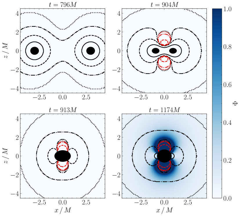
Figure 23: Snapshots of the scalar field, here labeled $\Phi$, and the $\mathscr{G}$ invariant in the $xz$-plane llustrating the phenomenon of spin-induced dynamical scalarization. The color map indicates the amplitude of the scalar field. The isocurvature contours are the same as Fig. 22. of the $\mathscr{G}$ invariant correspond to $1M^{-4}$ (solid line), $10^{-1}M^{-4}$ (dashed line), $10^{-2}M^{-4}$ (dot-dashed line), and $10^{-3}M^{-4}$ (dotted line). Black (red) lines correspond to positive (negative) values of $\mathscr{G}$. We show the inspiral (top left), half an orbit before merger (top right), formation of the first common apparent horizon (bottom left) and about $200M$ after the merger. Credit: Elley et al. [127].

A restriction of the decoupling limit is that it does not capture the backreaction of the scalar field onto the spacetime metric, thus not allowing one to derive the modifications to the gravitational-waves in the binary set-ups mentioned previously. These difficulties can be partially overcome by employing a formulation of the theory’s field equations in a generalized harmonic gauge, first developed by Kovács and Reall [192, 191] [see also Ripley [282]]. This formulation in principle allows one to evolve the complete scalar field and metric dynamics in scalar-Gauss-Bonnet gravity. However, the first binary BH coalescence simulations using this formalism in scalar-Gauss-Bonnet theories that allow for BH scalarization [126, 125] demonstrated that evolution ceases to be well-posed for larger values of the coupling. How different gauge choices and different models perform in this respect is not well explored yet.

Franchini et al. [133], motivated by going beyond the small-coupling approximation, explored fixing-the-equations approach to perform numerical simulations, an approach inspired by works in dissipative relativistic hydrodynamics [70]. The main idea is to modify the evolution equations of the theory, such that the short wavelength modes (with respect to some chosen scale) in the solution are somewhat controlled, while longer wavelength modes (associated to strong-coupling and the breakdown of well-posedness) become tractable. Franchini et al. [133] were able to use the formalism to study scalar field collapse in spherical symmetry in the scalarization model of Silva et al. [311]. This allowed them to evolve the system past situations were the original equations fail, due to appearance of regions in spacetime where the evolution changes character from hyperbolic to elliptic, which prevents further evolution of the system in time [283]. Moreover, the “fixed-equations” system evolves towards static BHs predicted by the original system of equations, thus indicating that it may provide a suitable “completion” of the original theory. Whether this approach remains valid in a situation with less symmetry, for example the case of BH binaries, remains to be explored.

Progress has also been made in modeling compact binary dynamics in the wider separation and lower velocities, i.e., in the domain of validity of PN theory. In particular, Shiralilou et al. [306, 307] extended to a general $f(\varphi)$ coupling the calculations of Yagi et al. [364], that applied for the shift-symmetric scalar-Gauss-Bonnet theory, i.e., $f(\varphi)\sim\varphi$. These works calculated the leading-order corrections due to curvature nonlinearities in the GW and scalar waveforms, finding that corrections due to the Gauss-Bonnet term appear at 1PN order in GWs. They also obtained the GW polarization and phasing. In addition, Julié and Berti [179] argued that during the adiabatic inspiral of two BHs, the Wald entropy of each BH is constant. This allows a precise definition of the “sensitivities” of BHs in scalar-Gauss-Bonnet gravity in terms of the variation of the ADM mass as a function of the ambient scalar field the BH is embedded in, at fixed Wald entropy. This parallels the notion that the baryonic mass of NSs is constant during the inspiral [88]. They also derived the two-body Lagrangian at 1PN order. Julié et al. [180] used this result in conjunction with the numerical calculation of sensitivities of spontaneously scalarized BHs to study binaries. They found that, in principle, BHs can evolve towards a situation in which the inner singularity approaches the event horizon of the BH before they merge. This suggest the possibility that, dependent on the model of scalar-Gauss-Bonnet gravity and the binary parameters, the field equations might simply not be able to predict a full binary evolution from inspiral to merger.

IV.2 Black hole scalarization in the presence of matter

Stefanov et al. [335] suggested the earliest model of BH scalarization which consisted of the DEF model coupled to nonlinear electromagnetism [334, 333]. They introduced a coupling between the scalar field and the Born-Infeld Lagrangian, and found that BH solutions with scalar hair branch-off from the general relativistic sequence of solutions. These BHs violate the no-scalar-hair theorems by Mayo and Bekenstein [216], Sen and Banerjee [301] which are valid for charged, nonrotating BHs in scalar-tensor theory. The bifurcation point occurs where the GR sequence of solutions becomes unstable to scalar perturbations [119].

A variety of scalarization models have been studied in Einstein-Maxwell theory following Herdeiro et al. [163], which introduced a coupling between the scalar field and the Lorentz invariant ${\cal F}^{2}=F_{\mu\nu}F^{\mu\nu}$ of the form $\exp(-\alpha\varphi^{2}){\cal F}^{2}$, where $\alpha$ is a dimensionless constant. In this model, BHs can scalarize, with ${\cal F}^{2}$ playing the role of the trace of the energy-momentum tensor in the NS scalarization in DEF-like models, or the Gauss-Bonnet invariant in BH scalarization models.

The simpler nature of the model allowed Herdeiro et al. [163] to perform numerical relativity simulations to study the scalarization process in the time-domain by expanding upon already available code bases [296, 295]. This allowed Herdeiro et al. [163] to show that the endpoint of the instability of the Reissner-Nordström BH is indeed a BH with scalar hair. Additional studies of this model were done by Fernandes et al. [132], Astefanesei et al. [29], Herdeiro et al. [159]. Within this model, Myung and Zou [240] studied the instability of the Reissner-Nordström solution, while Myung and Zou [238, 241], Blázquez-Salcedo et al. [51] analyzed the stability of the scalarized solutions. Fernandes et al. [131], Herdeiro and Oliveira [160] explored other variations of this theme, including scalar-axion couplings, i.e., $\propto h(\varphi)F^{\mu\nu}\tilde{F}_{\mu\nu}$, where $\tilde{F}_{\mu\nu}=(1/2)\epsilon\indices{{}_{\mu\nu}^{\alpha\beta}}F_{\alpha\beta}$ In addition, Ikeda et al. [175] considered the coupling between the double-dual of the Riemann tensor and $F_{\mu\nu}$.

Cardoso et al. [67, 68] explored a relevant scenario from an astrophysical perspective: matter in the vicinity of a BH could trigger scalarization and, in turn, endow the BH with scalar hair. They showed that this “matter-induced” scalarization (see Sec. II.3.3) is, in principle, possible for the DEF model. The viablility of this proposal in realistic matter configurations, such as an accretion disk or a dark matter halo, has not been explored yet. Matter-induced scalarization seems unlike to happen in light of the severe constraints on the DEF model. However, this might not be the case for other scalarization models, and the topic deserves further work.

After it was understood that in scalar-Gauss-Bonnet theories the Schwarzschild solution can scalarize, it was natural to ask if the same can happen to its charged counterpart, i.e., the Reissner-Nordström solution. Doneva et al. [106] analyzed this and found the existence of two bifurcation points, one at larger masses where the scalarized solutions bifurcated from the Reissner-Nordström one, and one at smaller masses where the scalar charge of the solution decreases again to zero and the branch merges again with the GR one. Scalarized charged BHs (in the fundamental mode) are also thermodynamically favored over the Reissner-Nordström solution. Brihaye and Hartmann [60] showed that for near-extremal Reissner-Nordström case, scalarization can happen for either sign of the scalar-to-Gauss-Bonnet couplings constant (35b). Other works varying the choice of the coupling function $f$ between the scalar field (or the axion field) and the Maxwell invariant, and studying the scalarization of dyonic BHs include Fernandes et al. [132], Fernandes et al. [131], Blázquez-Salcedo et al. [52] and Blázquez-Salcedo et al. [51].

Herdeiro and Radu [162] put forward a motivation to study these models. They noted that quantum effects can break the scale invariance and vanishing energy-momentum trace properties of electro-vacuum GR BHs. As a consequence, even the simplest nonminimally scalar field coupling $\xi\varphi^{2}R$ can result in BH scalarization when these quantum effects are taken into account. Within these models, they discussed the scalarization of the Reissner-Nördstrom solution and a noncommutative generalization of the Schwarzschild solution. They found that resultant scalarized BHs are, in general, entropically favored over the GR solutions.

IV.3 Variation of the curvature-induced scalarization model

In light of the nontrivial effect of rotation on scalarization, it is quite natural to consider what happens when Gauss-Bonnet invariant is replaced with the Pontryagin invariant ${}^{\ast}RR$ as the “curvature source”. The Pontryagin density is known to vanish in spherically symmetric spacetimes (such as that of Schwarzschild BH) and becomes nonzero for stationary and axisymmetric spacetimes (such as that of a Kerr BH). In this sense, all possible scalarized BHs in this theory are necessarily “spin induced”; a fact naturally shared with BH solutions in dynamical Chern-Simons gravity (see e.g., Yunes and Pretorius [373], Konno et al. [190], and Alexander and Yunes [9] for a review) which features a linear coupling between the scalar field and the Pontryagin invariant. We remark that the coupling between scalar field and Pontryagin density results in field equations with higher order derivatives (contrary to the case of Gauss-Bonnet) and, as such, these models are usually treated as EFTs, see e.g., Motohashi and Suyama [235], Delsate et al. [98]. Myung and Zou [239] studied the combined effect of Gauss-Bonnet and Pontryagin densities. In the test field limit, the scalar field dynamics with an effective mass proportional to $\phi^{2}\,{}^{\ast}RR$ was also studied in a Kerr background [139, 117] and in the Schwarzschild-NUT background [62].

Another extension of the original “Gauss-Bonnet” spontaneous scalarization model involves considering $n>1$ scalar fields $\varphi^{a}$, whose interaction is determined by their “target-space” $\gamma_{ab}(\varphi^{c})$, an $n$-dimensional Riemannian manifold [86, 169]. These are similar to the tensor-multi-scalar DEF models for NSs scalarization presented in Sec. III.4. In these models, the scalar field dynamics is determined by the quantity $\gamma_{ab}(\varphi)g^{\rho\sigma}\partial_{\rho}\varphi^{a}\partial_{\sigma}\varphi^{b}$. Doneva et al. [109] numerically obtained scalarized BH for the case $n=3$ and maximally symmetric target-space geometries. An important feature of these solution is that the scalar fields do not decay asymptotically as $1/r$ (i.e., the BHs do not have a monopole scalar charge). This shows that BHs in these theories will not emit dipole scalar radiation when placed in binaries.

V Generalizations of scalarization to other fields and instabilities

We identified the underlying reason for spontaneous scalarization in its various different forms to be a tachyonic instability. However, the scalar nature of the field did not have any special role in the mechanism. This suggests that other fields, e.g. vectors, might also spontaneously develop nontrivial configurations around compact objects when they exhibit suitable couplings to curvature. In this section, we will investigate this idea, which leads to the so-called spontaneous tensorization theories.

A second type of generalization of the spontaneous scalarization considers new types of instabilities as opposed to new types of fields. For instance, instead of replacing the scalar field with, say, a vector, replacing the tachyonic instability with, say, a ghost instability. We will see that a surprising key result of spontaneous tensorization is that these two paths are intimately connected. Namely, even if we only intend to have a theory of tachyons living on nonscalar fields, ghost and gradient instabilities necessarily arise in almost all models.

V.1 Spontaneous vectorization

What happens if we replace the scalar field of spontaneous scalarization with a vector? In scalarization, we started with the most general context in Sec. II.2.1, considering all the allowed couplings to the metric. Here we will follow the reverse path, starting with individual models of vector-tensor theories, and considering the more encompassing theory later. This exposition is preferable because the study of specific models, that are straightforward generalizations of known scalarization models, reveal some pathologies, and provides guidance for further model building.

The idea and the first specific model of vectorization was introduced in analogy with a massive version of the DEF model in Eq. (18). Consider the vector-tensor theory action [43, 266]

$$S =\frac{1}{16\pi G_{*}}\int{\rm d}^{4}x\,\sqrt{-g}\,\left[R-F^{\mu\nu}F_{\mu\nu}-2\mu_{X}^{2}x\right]$$

$$\quad+S_{{\rm m}}\left[\Psi_{{\rm m}};\,{\cal A}^{2}(x)g_{\mu\nu}\right],$$ (36)

where $F_{\mu\nu}=\nabla_{\mu}X_{\nu}-\nabla_{\nu}X_{\mu}$, $x=g^{\mu\nu}X_{\mu}X_{\nu}$. The vector field $X_{\mu}$ has the canonical kinetic term in this frame, and the matter degrees of freedom couple to the metric $\tilde{g}_{\mu\nu}={\cal A}^{2}(x)g_{\mu\nu}$ which is conformally scaled with respect to $g_{\mu\nu}$. The vector field equation is

$$\nabla_{\rho}F^{\rho\mu} =[-8\pi G_{*}{\cal A}^{4}\Lambda\tilde{T}+\mu_{X}^{2}]\,X^{\mu},$$ (37)

where $\Lambda\equiv{\rm d}\ln{\cal A}/{\rm d}x$, $T_{\mu\nu}$ is the energy-momentum tensor in the Einstein frame, and $\tilde{T}$ is the trace of the stress-energy tensor in the Jordan frame, i.e., with respect to the metric $\tilde{g}_{\mu\nu}$.

Equation (37) is that of a massive vector (Proca) field where the expression inside the square brackets acts as an effective mass $\mu_{\rm eff}^{2}$. In parallel to the DEF model, when $\cal A$ has an appropriate form, e.g. ${\cal A}=\exp(\beta_{0}x/2)$ with sufficiently negative $\beta_{0}$, $\mu_{\rm eff}^{2}$ becomes negative. Furthermore, for dense enough objects such as NSs, this occurs for order-of-unity values of $\beta_{0}$. The expectation is that the vector field grows from arbitrarily small perturbations around $X_{\mu}=0$ due to this tachyonic behavior, which can be called spontaneous vectorization, in exact analogy to spontaneous scalarization. However, we will later see that there are many subtle points in this narrative.

Even though we presented spontaneous vectorization in the Einstein frame with a nonminimal coupling to matter, it can be converted to a theory of minimal matter coupling and vector-curvature couplings as in spontaneous scalarization [270]. Even more directly, there are theories of spontaneous vectorization that are purely conceived through curvature coupling, the first example being the Hellings-Nordtvedt theory [158] studied by Annulli et al. [18]

$$S =\frac{1}{16\pi G}\int{\rm d}^{4}x\,\sqrt{-g}\,\left[R-F^{\mu\nu}F_{\mu\nu}-\Omega xR\right.$$

$$\quad\left.-\,\eta X^{\mu}X^{\nu}R_{\mu\nu}\right]+S_{{\rm m}}[\Psi_{{\rm m}};\,g_{\mu\nu}],$$ (38)

where $\Omega$ and $\eta$ are coupling constants. Scalarization through coupling to the Gauss-Bonnet term also has a vector analog as in the action [271]

$$S =\frac{1}{16\pi G}\int d^{4}x\sqrt{-g}\left[R-F^{\mu\nu}F_{\mu\nu}+f(x)\mathscr{G}\right]$$

$$\quad+S_{{\rm m}}[\Psi_{{\rm m}};\,g_{\mu\nu}],$$ (39)

which has a similar structure to Eq. (II.2.3). Action (V.1) leads to BH vectorization as well, unlike the other models we have seen so far.

The models of vectorization we have examined are only specific examples, and any theory of scalarization can be generalized to vector fields in principle. In this regard, Brihaye and Verbin [63] studied the coupling of a vector field to a scalar, and Oliveira and Pombo [249] and Brihaye et al. [61] studied the coupling between two vector fields to obtain vectorized compact objects. Kase et al. [183] considered generalized Proca theories [157, 343] with various different couplings of a massive vector field, and showed that spontaneous vectorization occurs in these models as well. Ramazanoğlu [268] investigated models where the effective mass of the vector field is generated by the Higgs-mechanism, preserving the gauge symmetry. On a separate front, conformal scaling of the metric in the matter action (V.1) can be generalized to disformal transformations, and spontaneous vectorization still occurs [274, 227]. In terms of approximate solutions, Garcia-Saenz et al. [141] recently calculated the Schwarzschild QNMs of nonminimally coupled vector fields. There have also been efforts to study all these phenomena in a unified manner in compact binaries, using more generic EFT tools [185].

To summarize, coupling of the vector field to any non-vanishing term in the action can be considered for spontaneous vectorization [271], and most options have been considered at least in a preliminary sense. The case of all possible couplings, an analog of the minimal action of scalarization in Sec. II.2.1, has also been studied by Garcia-Saenz et al. [140]. This work also revealed some of the fundamental problems of vectorization, as we will discuss more broadly later.

Vectorizations models strongly resemble scalarization models in terms of their actions, but this can be misleading. One major difference is in the number of additional degrees of freedom. Scalar fields contribute a single new degree of freedom irrespective of whether they are part of spontaneous scalarization or not, provided that the field equations are second order in derivatives. For vectorization, this is not the case. The action (37) and all the vector-tensor theory actions we have discussed break the gauge freedom found in massless vector fields. As a result, the vectors of vectorization models carry three degrees of freedom instead of the two found in electromagnetism. This is not an immediate reason of concern, since minimally coupled massive vectors, known as Proca fields [265], also break the gauge symmetry, and they still provide a classical field theory with well-behaved dynamics. However, as we will see, the extra degree of freedom is far more problematic in vectorization.

Although the vectorization models are designed to have a linear tachyonic instability in analogy with scalarization, the presence of the third degree of freedom, whose dynamics is not obvious, casts doubt on the success of this design. Namely, whether vectorization can indeed be described as a tachyonic instability of the vector modes, that is then quenched nonlinearly is not apparent. This concern is amplified by the fact that vectorized compact objects in the models studied so far seem to have some striking differences with respect to their scalarized counterparts.

As an example, consider vectorized BHs in the theory described by action (V.1). Entropy can be a measure of stability for BHs, where higher entropy solutions are favored in terms of stability. Entropy of spherically symmetric vectorized BHs were numerically computed by Barton et al. [35], and GR BHs were shown to be entropically favored over vectorized ones in all cases. The verdict of stability is not definite without time evolution, but this is a strong indication for the instability of vectorized BHs. In contrast, scalarized BHs in scalar-Gauss-Bonnet theories, e.g., Eq. (II.2.3), can be entropically favored to the ones in GR for appropriate coupling functions [113], and their stability is also indicated by other methods (see Sec. IV.1.2), which makes the stability of vectorized objects even more suspect.

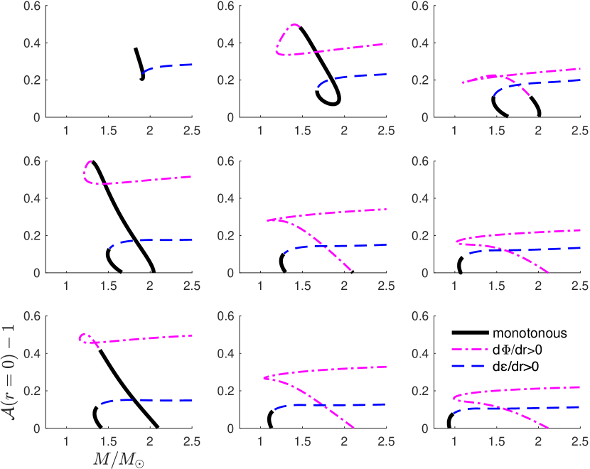
Figure 24: The strength of vectorization measured by ${\cal A}(r=0)-1$ as a function the NS mass $M$ for various values of $\beta_{0}$ and $\mu_{X}$ in Eq. (37). Rows: upper $\mu_{X}=1.6\times 10^{-11}$ eV, middle $\mu_{X}=8.0\times 10^{-12}$ eV, lower $\mu_{X}=4.8\times 10^{-12}$ eV. Columns: left $\beta_{0}=-4$, middle $\beta_{0}=-5$, right $\beta_{0}=-6$. Dashed and dot-dashed lines indicate solutions where the energy density $\varepsilon$ or $\Phi=-n^{\mu}X_{\mu}$ ($n^{\mu}$ being the normal vector field to spatial hypersurfaces) do not monotonically decrease with radius, respectively. Credit: Ramazanoğlu [266].

Scalarized and vectorized NSs also show major differences. For example, the dependence of the strength of vectorization on the NS mass has no discernible pattern as can be seen in Fig. 24, whereas scalarization occurs in a finite NS mass interval, and vanishes at the boundary mass values (see Fig. 1). It is also known that while scalarized NSs are continuously connected to those of GR as the theory parameters are smoothly changed, e.g. in the limit $\beta\to 0$ in Fig. 1, this is not the case in vectorization [266, 225]. The latter is known to be an indication of instability in certain scalarization theories, see Mendes and Ortiz [219]. Thus, qualitative differences between scalarized and vectorized objects are also apparent for NSs, and moreover, point to the instability of the vectorized ones.

These observations suggest that the vectorized compact object solutions obtained so far may not be stable, hence they are not astrophysically relevant, at least for the case of spherically symmetric spacetimes. A close look at the instability mechanism of vectorization is going to reveal the underlying reasons for this in the following section.

V.2 Vectorization and ghosts

Despite the fact that the vectorization phenomena we have presented are directly inspired by scalarization, we have seen noteworthy differences between the two mechanisms. Even though it was puzzling for a time, this is now strongly suspected to be related to the fact that vectorization models suffer from ghost and/or gradient instabilities in addition to tachyonic ones, as demonstrated by Garcia-Saenz et al. [140] and Silva et al. [308]. Here, we will first follow the latter, and later outline the methodology of the former.

Let us first review the basic aspects of different types of instabilities [99]. Recalling our discussion of the tachyon in Secs. II.1.1 and II.1.2, consider the linearized scalar field equation (5) in $1+1$ dimensions

$$g^{tt}\partial_{t}^{2}\delta\varphi+g^{xx}\partial_{x}^{2}\delta\varphi=\mu^{2}\varphi,$$ (40)

where we assume the metric is diagonal with constant components for simplicity. The common case without instabilities is when $g^{tt}<0$, $g^{xx}>0$, and $\mu^{2}>0$. What happens when each of these three terms changes its sign, while the other two stay the same?

For a plain wave mode $\delta\varphi(t,x)\propto\exp[{\rm i}\left(\omega t-kx\right)]$, the dispersion relation is given by

$$\omega(k)=\sqrt{(\mu^{2}+g^{xx}k^{2})/(-g^{tt})},$$ (41)

We saw that for $\mu^{2}<0$ the mode behaves as a tachyon, where $\omega(k)$ becomes imaginary for sufficiently small $|k|$. This leads to exponential growth as discussed, and the fastest growing mode behaves as $\sim\exp[\sqrt{\mu^{2}/g^{tt}}\,t]$, i.e., the growth rate has an upper limit.

A ghost occurs when $g^{tt}>0$. There is also exponential growth in this case, however the growth rate diverges with increasing wave number as $\sim\exp[\sqrt{g^{xx}/g^{tt}}kt]$, hence has no upper bound. The case $g^{xx}<0$ also gives the same asymptotic growth rate as the ghost, and is called a gradient instability. In summary, ghost and gradient instabilities as we presented them here have qualitative differences from tachyons, a main one being the arbitrarily fast growth rates. This means a well-defined time evolution can be problematic in such theories, and it is harder to devise nonlinear quenching mechanisms.

The spontaneous vectorization model of Eq. (V.1) modifies the “mass term” in the field equation for the vector field. Hence, the first impression might be that it leads to a tachyonic instability as in scalarization. However, this approach is naive, and a thorough analysis reveals that theories of vectorization necessarily carry ghost instabilities in addition to tachyonic ones. Following Silva et al. [308], one way to understand this is using the Stueckelberg trick [287] where we introduce a scalar field $\psi$ in the action (V.1) by the substitution

$$X_{\alpha}\to X_{\alpha}+\mu_{X}^{-1}\nabla_{\alpha}\psi.$$ (42)

This leads to the scalar equation of motion

$$\overline{\Box}\psi=-\bar{g}^{\mu\nu}\,[\,\mu_{X}\overline{\nabla}_{\mu}X_{\nu}+\tfrac{1}{2}(\overline{\nabla}_{\mu}\log\hat{z})(\overline{\nabla}_{\nu}\psi+\mu_{X}X_{\nu})\,].$$

where the covariant derivative $\overline{\nabla}$ is compatible with the new metric

$$\bar{g}^{\mu\nu}=\hat{z}\,g^{\mu\nu},\qquad\hat{z}\equiv\frac{\mu^{2}_{\rm eff}}{\mu_{X}^{2}}=1-\frac{8\pi G_{*}{\cal A}^{4}\Lambda\tilde{T}}{\mu_{X}^{2}}.$$ (44)

The signature of $\bar{g}_{\alpha\beta}$ changes with the sign of $\hat{z}$, which controls the change of sign of the effective mass of $X_{\mu}$ in Eq. (37). In other words, when we try to instigate a tachyon on $X_{\mu}$ by having negative $\hat{z}$ in parts of the spacetime, $\psi$ carries ghost and gradient instabilities [cf. Eq. (40)]. This is a degree of freedom whose dynamics is governed by the effective metric $\bar{g}_{\mu\nu}$, not the spacetime metric $g_{\mu\nu}$.

It is curious to see that the Stueckelberg trick reveals the ghost, even though it is not apparent in the vector field equation (37). However, a more careful analysis can clarify this issue [308]. First note that the vector field equation (37) is not manifestly hyperbolic, i.e. its principal part, the term with the highest derivatives, is not the wave operator, since

$$\nabla_{\mu}F^{\mu\nu}=\nabla_{\mu}\nabla^{\mu}X^{\nu}-\nabla_{\mu}\nabla^{\nu}X^{\mu}.$$ (45)

The second term on the right hand side of Eq. (37) vanishes for the Proca theory, ${\cal A}=1$, making the principal part the wave operator. This is not the case in general due to the so-called (generalized) Lorenz condition

$$\nabla_{\mu}\left(\hat{z}X^{\mu}\right)=0,$$ (46)

which is obtained by acting on both sides of Eq. (37) by $\nabla_{\mu}$, and recalling the antisymmetry of $F^{\rho\mu}$. We can use Eq. (46) to obtain a manifestly hyperbolic form of the linearized field equations on a fixed background of vanishing vector fields as

$$\nabla_{\mu}\nabla^{\mu}X_{\nu}+(\nabla_{\mu}\ln\hat{z})\nabla_{\nu}X^{\mu}=\mathcal{M}_{\nu\mu}X^{\mu},$$ (47)

where we defined the mass-squared tensor

$$\mathcal{M}_{\nu\mu}=\hat{z}\mu_{X}^{2}g_{\nu\mu}+R_{\nu\mu}-\nabla_{\nu}\nabla_{\mu}\ln|\hat{z}|.$$ (48)

Here, the metric and $\hat{z}$ have their fixed background GR values. This is a generalized massive wave equation.

Since $\hat{z}=1$ in the absence of matter, and it becomes negative in a continuous manner inside matter for an instability to exist at all, $\hat{z}$ necessarily vanishes at some points of a NS spacetime. The $\nabla_{\nu}\nabla_{\mu}\ln\hat{z}$ term introduced by the vectorization contains powers of $\hat{z}^{-1}$, which means the effective mass-squared tensor diverges at such points. Alternatively, if we move the $\hat{z}^{-1}$ terms to the other side of the equation, the principle part becomes $\hat{z}\Box X_{\nu}$, i.e. it changes its sign with $\hat{z}$ the same way as the $\psi$ field in equation (V.2). Hence, if we properly rewrite the vector field equation into a manifestly hyperbolic form, the ghost is apparent.

Equations (47) and (48) show that calling $\mu^{2}_{\rm eff}=\hat{z}\mu_{X}^{2}$ the effective mass squared of the theory is misleading, unlike the case of scalarization. Even though $\mu^{2}_{\rm eff}$ replaces the mass term in the vector field equation of a minimally coupled Proca field, it is not actually the effective mass of physically propagating degrees of freedom. The physical mass is determined by Eq. (48), which diverges at points where $\hat{z}=0$.

One might at first think that the ghost and gradient instabilities can be regularized by nonlinearities. After all, the tachyon of scalarization is also an instability, but it is eventually quenched by nonlinear effects as explained in Sec. II.1. In such a scenario, one would expect the vectorized objects to be free of instabilities, even though the GR solutions are unstable. However, this is not the case. Demirboğa et al. [99] showed that spherically symmetric vectorized NSs in the theory (V.1) are ghost and gradient unstable at the perturbative level.

Even if stable solutions can be found in other vectorization models, there is a more fundamental problem due to the modification to the principal part of the vector equations in Eq. (V.2) or (47). The coefficient of the wave operator vanishes at certain points in spacetime, or equivalently, the physical effective mass diverges if we move these coefficients to the other side of the equation. In either case, this leads to divergent time derivatives for arbitrarily small perturbative vector field values, which renders the initial assumptions of a perturbative approach invalid. Overall, it is not clear whether one can even define a well-posed time evolution, let alone one that can somehow suppress the exponential growth of the vector field [308]. Further elucidation of these issues requires a more rigorous mathematical investigation, which has not been attempted yet.

We have so far investigated the ghost and gradient instabilities of the specific vectorization theory in action (V.1), but similar results are known to exist for all theories of vectorization [140, 308] due to similar mechanisms. To summarize, replacing the scalar of scalarization with a vector field results in theories where the central issue is not the nature of the field the instability lives on, but the type of instabilities that arise. We cannot construct vectorization models that only exhibit the tachyonic instability commonly associated with the scalarization mechanism, which can be benign and tamed by nonlinear effects. Rather, vectorization also exhibits far more threatening instabilities.

Above, we closely followed Silva et al. [308], but Garcia-Saenz et al. [140] reach similar conclusions via an alternative approach. The authors consider the most general action that contains a vector field and the metric [157, 343], and truncate its action at the quadratic order around GR to obtain the linearized field equations. The main qualitative difference from the scalar minimal action of Sec. II.2.1 is that one can demonstrate that if any of the physical degrees of freedom has a tachyonic instability, then there are also degrees of freedom with ghost or gradient instabilities, which are manifested by change of sign of coefficients in the dispersion relationship. The conclusion is the same: vectorization based on tachyonic instabilities necessarily has ghost or gradient instabilities as well.

Recent works showed that the issues with vectorization also happen in simpler theories, an example being minimally coupled self-interacting vector field theories. For instance, for $\mathcal{A}(x)=1$ the action (V.1) becomes the minimally coupled Proca theory, which is well-posed. However, generalizations of the potential beyond a mass term, that is $2\mu_{X}^{2}x\to 4V(x)$ for some generic function $V$, results in ill-posedness [236, 79, 81]. The underlying reason is the fact that there is an analog of the generalized Lorenz condition (46) in this case as well, which ultimately leads to the same result: there is a degree of freedom in the theory whose dynamics is governed by an effective metric, an analog of $\bar{g}_{\mu\nu}$ in Eq. (44). This new metric depends on the vector field itself, and can lose its Lorentzian nature depending on how $X_{\mu}$ evolves in time [81].

Esposito-Farèse et al. [130] provided some of the earliest examples of the ill-posedness of self-interacting vector field theories we mentioned above in a cosmological context, and it was recently demonstrated that initially healthy configurations of self-interacting vectors naturally evolve to a point where hyperbolic evolution becomes impossible [236, 79, 81]. This means, nonlinear extensions of the Proca theory are more delicate than their scalar counterparts in terms of providing physical theories. It seems that the underlying reason for the “failure” of vectorization is a much more general phenomenon in theories with conditions such as Eq. (46), at least for the models conceived thus far. In this sense, exploration of vectorization has been leading to a deeper understanding of vector fields in general, which has implications beyond theories of gravitation.

We close this section with a pertinent comment on ghost instabilities. We encountered them as an unappealing artefact in vectorization theories, but one could consider making them the driver of a spontaneous growth mechanism. This option has indeed been considered prior to their discovery in vectorization models. The simplest example is another analog of the DEF model where the conformal scaling function ${\cal A}$ depends on derivative terms [267]

$$S =\frac{1}{16\pi G_{*}}\int d^{4}x\sqrt{-g}\left[R-2g^{\mu\nu}\partial_{\mu}\varphi\partial_{\nu}\varphi-2\mu^{2}\varphi^{2}\right]$$

$$\quad+S_{{\rm m}}[\Psi_{{\rm m}};{\cal A}^{2}(K)g_{\mu\nu}],$$ (49)

with $K=-g^{\mu\nu}\partial_{\mu}\varphi\partial_{\nu}\varphi/2$. The scalar equation of motion is

$$\nabla_{\mu}\left(\hat{z}\nabla^{\mu}\varphi\right)=\mu^{2}\varphi,$$ (50)

where $\hat{z}\equiv 1+4\pi G_{*}\tilde{T}{\cal A}^{4}\left({\rm d}\ln{\cal A}/{\rm d}K\right)$. Unlike the tachyonic instability where the mass term is modified, the derivative terms are modified in this case.

The nature of Eq. (50) can be better understood when we consider the linearized equation for perturbative values of the scalar around a GR background, and highlight the principal part as

$$\hat{z}\,\Box\delta\varphi+\dots=0.$$ (51)

For an appropriate choice such as ${\cal A}=\exp(\beta_{0}K)$ with large enough $\beta_{0}>0$, the sign of $\hat{z}$ can become negative in the presence of matter. In all spontaneous scalarization theories considered so far, the source of the instability was the change of sign of the effective mass term, which resulted in a tachyon. Here, the overall sign of the wave operator changes, hence we have both ghost and gradient instabilities, recalling Eq. (40) and the subsequent discussion. Spontaneous scalarization that might arise from this new mechanism is called ghost-based spontaneous scalarization [267]. It has similar problems as vectorization, in that it is hard to tame the ghost and other instabilities, hence we do not end up with a theory with sensible dynamics.

V.3 Spontaneous tensorization

The basic mechanism of spontaneous scalarization can be generalized beyond vector fields, resulting in spontaneous tensorization. However, all known such theories also feature ghosts and suffer from similar problems with vectorization, aside from a single possible example of spinor-tensor theory.

The simplest mathematical generalization of scalarization beyond vectors occurs for $p$-form fields, i.e., totally antisymmetric tensors $X_{\mu_{1}\dots\mu_{p}}$ of rank $(0,p)$. This is due to the fact that a vector field $X_{\mu}$ is a $1$-form field, and the actions we encountered in spontaneous vectorization can be readily generalized to this class of fields as [272]

$$S =\frac{1}{16\pi}\int{\rm d}^{4}x\,\sqrt{-g}\,\left[R-F_{\mu_{1}\dots\mu_{p+1}}F^{\mu_{1}\dots\mu_{p+1}}\right]$$

$$\quad+S_{{\rm m}}\left[\Psi_{{\rm m}};\,{\cal A}^{2}(x)g_{\mu\nu}\right],$$ (52)

where $F_{\mu_{1}\dots\mu_{p+1}}=(p+1)\nabla_{[\mu_{1}}X_{\mu_{2}\dots\mu_{p+1}]}$, with square brackets denoting antisymmetrization, and $x=X_{\mu_{1}\dots\mu_{p}}X^{\mu_{1}\dots\mu_{p}}$. It is then straightforward to show that the analog of $\mu^{2}_{\rm eff}$ becomes negative inside NSs for an appropriate choice of ${\cal A}(x)$. However, these theories carry ghost instabilities similar to those of vectors when we try to establish spontaneous growth from tachyonic instabilities, since they possess an analog of the Lorenz condition (46) [308].

Spontaneous tensorization of a symmetric rank $(0,2)$ tensor field $f_{\mu\nu}$, which is spin-$2$, is a natural avenue to investigate after spin-$0$ (scalars) and spin-$1$ (vectors). Ghosts appear in this case once more since the metric in our gravity theories, $g_{\mu\nu}$, is also a spin-$2$ field. Note that spontaneous tensorization theories include terms where the field that tensorizes, in this case $f_{\mu\nu}$, is coupled to the metric $g_{\mu\nu}$. However, interacting spin-$2$ fields are known to generically lead to ghost degrees of freedom, rendering most such theories unphysical [58, 277], and ghost-free theories being discovered more recently in the form of massive gravity and bigravity [278, 155, 277]. Matter can couple to one of the spin-$2$ fields in the novel ghost-free theories, but coupling to both metrics generically invoke a ghost again [369]. For example, trying to mimic the DEF model by having a conformal scaling function that depends on $f_{\mu\nu}$, i.e., changing the matter action as $g_{\mu\nu}\to{\cal A}(f_{\mu\nu},g_{\mu\nu})\ g_{\mu\nu}$, leads to ghosts. Overall, there is no known form of bigravity theory that features an analog of spontaneous scalarization.

Spinor fields present the most interesting case of generalizing scalarization, perhaps aside from vectors. The classical Lagrangian for a Dirac spinor is

$$\mathcal{L}_{\psi}=\tfrac{1}{2}\left[\bar{\psi}\gamma^{\mu}(\nabla_{\mu}\psi)-\nabla_{\mu}\hat{\gamma}^{5}\gamma^{\mu}\psi\right]-\mu\bar{\psi}\psi,$$ (53)

where the conventions for gamma matrices and the effect of covariant derivatives on spinors can be found in Ramazanoğlu [269]. This action provides the usual dispersion relation $\omega^{2}=k_{i}k^{i}+\mu^{2}$ for a plane wave of the form $\psi\propto\exp[{\rm i}(\omega t-k_{i}x^{i})]$. Since the mass term appears linearly, not quadratically, changing its sign results in the same dispersion relation. However, a tachyonic spinor action is still possible in the form of

$$\mathcal{L}_{\psi}^{5}=\tfrac{1}{2}\left[\bar{\psi}\hat{\gamma}^{5}\gamma^{\mu}(\nabla_{\mu}\psi)-(\nabla_{\mu}\bar{\psi})\hat{\gamma}^{5}\gamma^{\mu}\psi\right]-\mu\bar{\psi}\psi.$$ (54)

with the field equation

$$\gamma^{\mu}\nabla_{\mu}\psi-\hat{\gamma}^{5}\mu\psi=0.$$ (55)

Here, $\omega^{2}=k_{i}k^{i}-\mu^{2}$, that is, the dispersion relation is tachyonic [76, 178].

Ramazanoğlu [269] used Eq. (54) to obtain the first spontaneous spinorization theory where spinor fields are unstable to growth around GR backgrounds of NSs. Even though the meaning of a ghost as opposed to a tachyon is a subtle issue for spinors, the equation of motion in this theory has divergent coefficients as in the vector field case (47), hence this form of spinorization suffers from similar problems to vectorization.

Minamitsuji [226] proposed an alternative model of spinorization given by the action

$$S =\frac{1}{16\pi G_{*}}\int{\rm d}^{4}x\,\sqrt{-g}\,\left\{R+\tfrac{1}{2}\left[\bar{\psi}\hat{\gamma}^{5}\gamma^{\mu}(\nabla_{\mu}\psi)\right.\right.$$

$$\quad\left.\left.-\,(\nabla_{\mu}\bar{\psi})\hat{\gamma}^{5}\gamma^{\mu}\psi\right]\right\}+S_{\rm m}\left[\Psi_{{\rm m}},\,{\cal A}^{2}(\bar{\psi}\psi)g_{\mu\nu}\right].$$ (56)

This model has the unusual feature that the derivative part of the spinor action is not the canonical one in Eq. (53), but rather the “tachyonic” one in Eq. (54). The resulting tachyonic equation of motion is

$$\gamma^{\mu}\nabla_{\mu}\psi-\hat{\gamma}^{5}(4\pi{\cal A}^{4}\Lambda\tilde{T})\psi=0,$$ (57)

where $\Lambda={\rm d}\ln{\cal A}/{\rm d}(\bar{\psi}\psi)$. The interpretation is straightforward, we have a tachyonic field with an effective mass $\mu_{\rm eff}=4\pi{\cal A}^{4}\Lambda\tilde{T}$ [cf. Eq. (55)]. The most important aspect of this theory is the fact that the effective mass term and all coefficients of the field equation are regular everywhere, hence, the dynamics does not have any signs of ill-posedness that we have found in all generalizations of scalarization so far. In other words, action (57) is the only known analog of spontaneous scalarization for non-scalar fields that does not suffer from ghost or gradient instabilities.

Our results on spontaneous tensorization suggest a no-go theorem for generalizing scalarization beyond scalar fields, at least if we want to avoid ghosts. It is curious to find the only exception to this trend in the relatively exotic case of spinorization, which invites studies of the deeper reasons that make spontaneous scalarization hard to replicate for other types of fields.

VI Open problems and future perspectives

We chose to review the literature by starting from the theoretical underpinning of the scalarization mechanism, then moving on to discussing NSs and BHs separately, and then returning to model building in order to discuss generalization of the mechanism to other fields. Most, but not all, open problems have come up already within one or more of the previous sections and discussed to some extent. Nevertheless, we will use this section to revisit them and cover any additional areas that require further development, opting to a concise summary of future perspectives.

VI.1 Scalarization and cosmology

As already discussed in Sec. II.2.4, one of the key challenges for scalarization is understanding whether it is compatible with cosmology. Recall that the main premise of scalarization is that there exists some constant value of the scalar field, $\varphi_{0}$, for which spacetimes of GR become admissible solutions to the field equations and it is these solutions that describe stationary objects that we expect (from an observational perspective) to carry no scalar charge. For this to be true, cosmic evolution needs to comply and drive $\varphi$ to $\varphi_{0}$ in the late universe, or else the whole universe will in effect be “scalarized.” It has been pointed out early on by Damour and Nordtvedt [91] and more recently by Anderson et al. [15], Franchini and Sotiriou [135] that reaching this preferred value for the scalar fields in the late universe is not generic for simple models of scalarization and instead requires severe fine-tuning of initial conditions.

This could well be an artefact of not having the complete theory and, ideally, one would expect the need to fine-tuned initial conditions to disappear by addressing further corrections to the model. A first step in this direction has been made by Antoniou et al. [24], inspired by Damour and Nordtvedt [91], by showing that the “mixed” model of scalarization discussed in Sec. II.2.4 has GR with a constant scalar as a late-time cosmic attractor for the right sign of the coupling between the scalar and the Ricci scalar. This demonstrated that, in principle, scalarization models can be made compatible with late-time cosmology and provided a recipe for doing so: include in the action terms that will dominate in late cosmology (e.g., Ricci coupling) over the terms that control the onset of scalarization (e.g., Gauss-Bonnet invariant) and hence impose the desired cosmological behavior. However, the specific model discussed as an example in Antoniou et al. [24] is by no means unique, and there are many other attempts to address similar concerns [72, 231, 128]. Perhaps more importantly, understanding the efficiency of the attractor behavior in reproducing the behavior of GR (with a cosmological constant) quantitatively, down to evolution of perturbations, structure formations, etc. certainly deserves further investigations and could lead to constraints on realistic models of scalarization.

A second point of friction between scalarization and cosmology relates to the early universe. Broadly speaking, scalarization is controlled by the coupling between the scalar field and curvature invariants, so it is inevitable that these couplings will become increasingly important as one runs cosmic evolution backwards and move to higher and higher curvatures. In particular, they will tend to dominate when the size of the universe will become comparable to the size of the compact objects we want scalarization to affect today (see e.g. Antoniou et al. [24]). It has been pointed out by Anson et al. [20, 21] that quantum fluctuations could then seed a scalarization-like instability during inflation and that it would be hard to prevent this (linear) instability by adding corrections to the action. It should however be stressed that one does not need the scalar to necessarily remain constant or have its current value through the evolution of the universe. Hence one might not need to prevent such an instability, but instead just quench it nonlinearly, exactly as it happens in scalarization itself. The scalar could then smoothly evolve away from the vacuum that leads to this instability before it becomes relevant, as one moves backwards in cosmic time. The key question here is whether there exists an EFT applicable to the early universe, which contains the scalarization models as late universe limits, but can also host an inflationary scenario compatible with observations.

As a final remark in relation to cosmology, we should emphasize that we have discussed here only the cosmological implications of known scalarization models and only under the assumption that the scalar field is cosmologically subdominant at late times. There is clearly a plethora of generalized scalar-tensor theories that have been used in the context of inflation or dark energy, which exhibit couplings between the scalar and curvature invariants similar to those employed for scalarization models, but in most cases the nature of the couplings differ quite significantly from those of scalarization models. Reviewing such attempts goes well beyond the scope of this manuscript. Exploring whether a scalar field that exhibits scalarization around compact objects could also play a role on inflation or account for dark energy would certainly be interesting, but putting together such a model (with a single scalar) seems particularly challenging. It is worth mentioning in this context that evading constraints on the coupling between a scalar and the Gauss-Bonnet invariant coming from the speed of GWs does require the scalar to be cosmologically subdominant [135].

VI.2 Dynamical evolution

The study of the dynamical nonlinear regime of scalarization requires nonperturbative time-evolution schemes, whose availability varies between models. Finding formulations of gravity theories that are amenable to numerical time evolution, i.e., numerical relativity, is nontrivial even in GR [264, 66, 31], and the issue can become even more complicated for alternative theories.

Time-domain, nonlinear evolution of DEF-like models have been done since the early days by Novak [246, 245], Novak and Ibanez [247], and binary inspirals have been performed for nearly a decade [33]. This was possible thanks to the relative simplicity of the field equations that allows one to establish their well-posedness [290, 291]. However, detailed and fully nonlinear numerical results in relation to GWs, a primary tool to test scalarization, are still few, such as the study by Shibata et al. [305].

The picture is quite different for BH scalarization where the coupling to the Gauss-Bonnet term can result in a complicated causal structure of the spacetime in dynamical situations. It was demonstrated both at linear [49, 47, 48] and nonlinear [125, 126, 283] levels that, part, but not all, of the parameter space of spontaneous scalarization where scalarized BHs can be found loses hyperbolicity when the theory is evolved in time in a certain set of gauges, which means that no predictions can be obtained. For the moment, there is no consensus on whether this loss of hyperbolicity can be cured by a better gauge choice or if it is intrinsic to the evolution equations, which calls for further work on the issue. Furthermore, there are no detailed studies of binary evolution and merger even for the part of the parameter space for which hyperbolic time evolution has been shown to exist. The dynamics of more general models where various coupling terms are present as in Eq. (II.2.1) are not available either. The lack of results on all these fronts presents important future research directions.

It can be the case that an EFT, obtained as a certain limit or truncation of a more fundamental theory, is ill-posed while the latter is or is expected to be well-posed. A typical example is relativistic hydrodynamics once viscocity has been taken into account. Indeed, it has been suggested to introduce techniques used in hydrodynamics to gravity in order to render the problematic time evolution of some theories hyperbolic by suitably modifying the equations, while keeping the end point of evolution the same [70]. This approach has seen increasing use in alternatives to GR, including the specific case of scalar-Gauss-Bonnet theories under certain symmetries [133], and it is another avenue to explore the dynamics of scalarization in cases where current methods are inadequate. The applicability and power of such methods to general cases, e.g., fully nonlinear 3+1 evolution of a highly dynamical system, are yet to be confirmed.

VI.3 Model building in and beyond scalarization

We have covered several models of spontaneous scalarization and their phenomenology for NSs and BHs. What they all have in common is that scalarization is triggered by a tachyonic instability, whose threshold is controlled by less than a handful of terms in the action [17]. Yet, the properties of the final scalarized configuration depend quite delicately on the nonlinearities and coupling terms that contribute beyond the linear level. The specific choices of these nonlinear interactions have been shown to crucially affect the stability [49, 311, 26] and the scalar charge [311, 212, 25, 106] of scalarized solutions, as well as the cosmological behavior of the corresponding theory [24, 20, 128]. Thus it is clear that such choices affect viability and observability of the models. As a result, although certain models of scalarization, such as the original DEF model, have been studied fairly exhaustively, the exploration of the broader class of theories that exhibit scalarization, and their phenomenology, has only started.

Furthermore, one could consider introducing new classes of scalarization based on instabilities that are not tachyonic in nature. As discussed in Sec. V, so far success in this direction is limited but it is nevertheless an existing prospect. Alternatively, one can abandon the idea of a linear instability quenched by nonlinearities altogether as we discussed in Sec. II.3.5. It was recently demonstrated in Doneva and Yazadjiev [118] that a theory that features a $\varphi^{4}$ coupling to the Gauss-Bonnet invariant can still have scalarized BHs below a certain mass threshold, although the Kerr solution is linearly stable with respect to (massless) scalar perturbations [50]. Such observation remains true in more general theories, such as Gauss-Bonnet gravity with multiple scalar fields [329]. This strongly suggests the existence of a class of theories in which scalarization is a purely nonlinear phenomenon.

Scalarization models that have been considered so far typically assume that the scalar field does not couple to matter directly in a suitable choice of variables, usually called the Jordan frame, which suffices for the theory to satisfy the WEP. However, as pointed out in Coates et al. [80], this assumption might not be necessary because scalarization itself forces the scalar field into a trivial configuration away from a specific compact object. Therefore, scalarization models can be indistinguishable from GR for what regards the WEP for all current observations. It was further argued in Coates et al. [80] and Franchini et al. [134] that particular couplings to matter that do not disrupt scalarization could introduce a Higgs-like mechanism in gravity: the scalar field changes value only near compact objects, and its coupling to matter changes the properties of the Standard Model in these regions. This is a largely unexplored possibility.

As was discussed in detail in Sec. V, another important open question is whether one can generalize the scalarization mechanism to other fields. Doing so in a context of a theory that is free of pathologies has so far proven to be quite challenging, except perhaps for the case of spinors [226]. This is in part because controlling the dynamics of the extra degree of freedom is notoriously difficult in general in gravity theories with additional vector or tensor fields [277], and vectorization or tensorization models are no exception.

We should stress that the work on scalarization, or its extensions, has focused on isolated compact objects. In fact, theoretical considerations for putting together scalarization models have also been heavily influence by studies of isolated BHs and NSs. However, as we discussed already above, scalarization could happen dynamically in a binary [33, 251, 305, 342, 127, 314, 110]. Apart from finding ways to model this effect [184] and potentially constraining it with GW observations (see also below), it would be particularly interesting to explore further what properties of a binary control dynamical scalarization, and how this differs between different scalarization models.

VI.4 Observational prospects

Perhaps the most attractive feature of scalarization is that the tachyonic instability typically leads to large scalar field amplitudes before it is quenched, which leads to nonperturbative deviations from GR in high curvature regions. At the same time, the theory mimics GR closely for weak gravity, easily satisfying existing tests. This suggests that new fundamental scalar that exhibit this behavior could be discovered with strong gravity observations.

Current observations put stringent bounds on scalar radiation from pulsars, which have already almost completely ruled out the original (massless) DEF model [378]. Electromagnetic observations of compact objects in binaries or surrounded by some form of matter also have the potential to extend such results to more general models of scalarization. For example, x-ray data from NS surfaces have been recently considered as a possible way to detect scalarized objects [316, 315]. The masses, radii and moment of inertia of NSs can be inferred through such observations [55, 56, 57]. Future observation could be used to distinguish scalarized NSs from nonscalarized ones, for instance, using EOS-independent relations. The astrophysical signatures of most extensions of the DEF model, especially those that allow BH scalarization have not been studied in details yet, because they are recent.

The most exciting current development in strong gravity is the advent of GW astronomy, which is an arena for exploring spontaneous scalarization. Effects of scalarization on GWs of coalescing NSs and/or BHs have been investigated to some extend, mostly for the DEF model [302, 185, 184, 244] and scalar-Gauss-Bonnet gravity [361]. The most pressing issue in this front is the development of accurate waveform models, that ideally would cover the inspiral, merger and ringdown stages of coalescing binaries. Developing such waveform models in GR has been (and remains) a formidable task that combines tools from post-Newtonian theory, numerical relativity, black-hole perturbation theory, and gravitational self-force. Progress in all these fronts are necessary in order for one to have accurate “scalarized” waveform models. Stars that undergo core collapse are another interesting source of GWs. Albeit expected to be rare, such events may produce large bursts of scalar radiation [328, 284, 200] and may contribute to the stochastic GW background which could, in principle, be probed by pulsar timing arrays. In addition, some model of scalarization (but not exclusively) predict the existence of extra polarizations in GWs, which provides another way to test them.

Last but not the least, future space-borne GW detectors such as LISA will bring another channel for testing modified gravity. Especially interesting with respect to scalarization is the case of extreme mass-ratio inspirals when the secondary object is scalarized [214, 215]. Data from future GW detectors, such as LISA, or third generation ground-based detectors, such as the Einstein Telescope and the Cosmic Explorer, combined with more precise electromagnetic observations, such as those from improved x-ray observatories, will be crucial for detecting or ruling out scalar fields that exhibit scalarization.