Functional Determinant Approach Investigations of Heavy Impurity Physics

Abstract

In this brief review, we report some new development in the functional determinant approach (FDA), an exact numerical method, in the studies of a heavy quantum impurity immersed in Fermi gases and manipulated with radio-frequency pulses. FDA has been successfully applied to investigate the universal dynamical responses of a heavy impurity in an ultracold ideal Fermi gas in both the time and frequency domain, which allows the exploration of the renowned Anderson’s orthogonality catastrophe (OC). In such a system, OC is induced by the multiple particle-hole excitations of the Fermi sea, which is beyond a simple perturbation picture and manifests itself as the absence of quasiparticles named polarons. More recently, two new directions for studying heavy impurity with FDA have been developed. One is to extend FDA to a strongly correlated background superfluid background, a Bardeen–Cooper–Schrieffer (BCS) superfluid. In this system, Anderson’s orthogonality catastrophe is prohibited due to the suppression of multiple particle-hole excitations by the superfluid gap, which leads to the existence of genuine polaron. The other direction is to generalize the FDA to the case of multiple RF pulses scheme, which extends the well-established 1D Ramsey spectroscopy in ultracold atoms into multidimensional, in the same spirit as the well-known multidimensional nuclear magnetic resonance and optical multidimensional coherent spectroscopy. Multidimensional Ramsey spectroscopy allows us to investigate correlations between spectral peaks of an impurity-medium system that is not accessible in the conventional one-dimensional spectrum.

I Introduction

An important approach to investigating polaron physics is to study the heavy impurity limit. Infinitely heavy impurity interacting with a Fermi sea represents one of the rare examples of exactly solvable many-body problems in the nonperturbative regime, which can serve as a benchmark for various approximations. Historically, this problem originated from the studies of the x-ray spectra in metals, where Mahan predicts the so-called Fermi edge singularities (FES), absorption edges in the spectra characterized by a power law divergence near the threshold Mahan (2000). The optical transition is determined by a highly spatial localized core-level hole that can be regarded as an impurity with infinite mass immersed in a Fermi sea of conduction electrons. The corresponding model Hamiltonian can be solved exactly and is often called MND Hamiltonian in the condensed matter community after the work of Mahan Mahan (1967a, b) and Noziéres-De Dominicis Nozières and De Dominics (1969).

FES is the first and one of the most important examples of nonequilibrium many-body physics. The underlying physics can be interpreted by the concept of Anderson’s orthogonality catastrophe (OC) Anderson (1967), i.e., the many-particle states with and without impurity become orthogonal. FES has also been observed in current-voltage characteristics of resonant tunneling experiments dominated by localized states Matveev and Larkin (1992); Geim et al. (1994) and has been proposed to be investigated in various systems, including quantum wires Ogawa et al. (1992); Prokof’ev (1994); Komnik et al. (1997), and quantum dots Bascones et al. (2000). In particular, a convenient and numerically exact method, namely the functional determinant approach (FDA) Levitov and Lee (1996); Klich (2003); Schönhammer (2007); Ivanov and Abanov (2013), has been developed to study FES in out-of-equilibrium Fermi gases Muzykantskii et al. (2003); d’Ambrumenil and Muzykantskii (2005); Abanin and Levitov (2005) and open quantum dots Abanin and Levitov (2004). Using FDA to investigate MND Hamiltonians has also been applied to study exciton-polarons in monolayer transition metal dichalcogenides (TMD), where the exciton serves as the impurity, and the itinerant excess electrons play the role of the background Fermi sea Chang and Reichman (2019); Lindoy et al. . However, the prediction can only be considered qualitative here, as the exciton mass is only about twice the electron mass in TMDs.

In recent years, ultracold quantum gases have emerged as an ideal testbed for impurity physics thanks to their unprecedented controllability. In the context of ultracold Fermi gases, the FES of an infinitely heavy impurity in an ideal Fermi gas has been quantitatively re-examined via the FDA Knap et al. (2012); Schmidt et al. (2018a) and can be verified via Ramsey-interference-type experiments Goold et al. (2011). The Ramsey signals in the time domain are universal, i.e., fully determined by the impurity-medium scattering length and the Fermi wave vector of the medium Fermi gases, not only in the long-time limit (as their counterpart in solid-state systems) but also for all times. Corresponding spectra in the frequency domain obtained by Fourier transformation show FES and provide an insightful understanding of polaron physics. The exact results of the FDA can serve as benchmark calculations for various approximation calculations of Fermi polarons, such as Chevy’s ansatz or equivalently many-body T-matrix Chevy (2006); Combescot et al. (2007); Punk et al. (2009); Cui and Zhai (2010); Mathy et al. (2011); Schmidt et al. (2012); Parish and Levinsen (2013); Levinsen et al. (2015); Hu et al. (2016, 2018); Mulkerin et al. (2019); Parish et al. (2021), and other exact methods, such as quantum Monte Carlo methods Lobo et al. (2006); Kroiss and Pollet (2015); Goulko et al. (2016); Pessoa et al. (2021).

However, polaron, strictly speaking, does not exist in the infinitely heavy impurity limit, where the quasiparticle residue of polaron vanishes due to the presence of OC Knap et al. (2012); Schmidt et al. (2018a). On the other hand, the generalization of the FDA to finite impurity mass remains elusive. Nevertheless, FDA has been proven to be qualitatively accurate in describing heavy polarons in ultracold Fermi gases at a finite temperature, where thermal fluctuation is comparable with recoil energy Cetina et al. (2016); Liu et al. (2019). In addition, one can choose an impurity with very different polarizability from the background fermions. As a result, the impurity can be confined by a deep optical lattice or an optical tweezer without affecting the itinerant background fermions. In this case, the infinitely heavy mass limit becomes exact, and FDA calculations can serve as a critical meeting point for theoretical and experimental efforts to understand the complicated quantum dynamics of interacting many-particle systems. Inspired by the pioneer works Knap et al. (2012); Schmidt et al. (2018a), a heavy impurity in Fermi gases has also been proposed to investigate spin transportation You et al. (2019) and precise measurement of the temperature of noninteracting Fermi gases Mitchison et al. (2020). The exact finite-temperature free energy and Tan contact Braaten et al. (2010), as well as the exact dynamics of Tan contact of a heavy impurity in ideal Fermi gases, can be derived as a generalization of FDA Liu et al. (2020). Rabi oscillations of heavy impurities in an ideal Fermi gas can also be investigated via FDA Adlong et al. (2021). Extensions of the FDA to the investigation of Rydberg impurities Balewski et al. (2013); Wang et al. (2015) in Fermi Sous et al. (2020) and Bose gases Schmidt et al. (2016); Camargo et al. (2018); Schmidt et al. (2018b) have also been developed recently.

Here, we briefly review the formalism of the FDA and two recent developments. Firstly, FDA has been generalized to the system of a heavy impurity in a Bardeen–Cooper–Schrieffer (BCS) superfluid, where the strongly correlated superfluid background is described by a BCS mean-field wavefunction Wang et al. (2022a, b). In contrast to the ideal Fermi gas case, the pairing gap in the BCS superfluid prevents the OC and leads to genuine polaron signals in the spectrum even at zero temperature. In addition, at finite temperature, additional features related to the subgap Yu-Shiba-Rusinov (YSR) bound state ware predicted in the spectra of a magnetic impurity. Another recent development is to extend the FDA to multidimensional (MD) spectroscopy. In contrast to conventional one-dimensional (1D) spectroscopy which depends only on one variable, such as photon frequency, MD spectroscopy unfolds spectral information into several dimensions, revealing correlations between spectral peaks that the 1D spectrum cannot access.

II Formalism

II.1 System setup

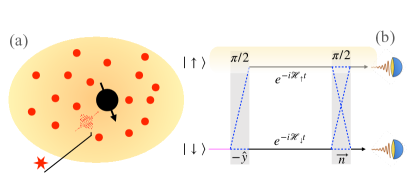
Figure 1: (a) A sketch of the system setup for 1D Ramsey spectroscopy (injection scheme). (b) An interferometry interpretation of 1D Ramsey spectroscopy.

The basic setup of our system is shown in Fig. 1 (a). We place a localized fermionic or bosonic impurity (the big black ball with a black arrow) with two internal pseudospins states $|\uparrow\rangle$ and $|\downarrow\rangle$ , which we will call spins for short from now on, in the background of ultracold Fermi gas (the red dots). In real experiments, there is usually more than one impurity, but the impurity density is prepared to be very low so that the interaction between impurities can be regarded as negligible. As mentioned before, the localization of impurity can be either achieved by confinement of a deep optical trap or treated as an approximation to an impurity atom with heavy mass. Unless specified otherwise, we are interested in the case where the interaction between the background Fermi gas and $|\downarrow\rangle$ is negligible, while the interaction with $|\uparrow\rangle$ is arbitrarily tunable by, e.g., Feshbach resonances. (It is straightforward to generalize to the case where both $|\uparrow\rangle$ and $|\downarrow\rangle$ interact with the background.) The spins states can be manipulated by radio-frequency (RF) pulses, which assume to be able to rotate the spins infinitely fast. In reality, the RF pulse length is usually comparable with the characteristic time scale $\tau_{F}=E_{F}^{-1}$ of the background Fermi gases, where $E_{F}$ is the Fermi energy, and we use unit $\hbar=1$ throughout this work. For example, in Ref. Cetina et al. (2016), the typical pulse length is about $10$ $\mu$s, approximately $3.4$ $\tau_{F}$ in their system. However, the optical control of Feshbach resonances in their experiment can be achieved very rapidly in less than $200$ ns, which is about 0.08 $\tau_{F}$. As a result, one can switch off the interaction (for both spin states) in no time and rotate the spin without perturbing the background Fermi gas, which can be treated as an infinitely fast rotation theoretically. The interaction is switched back on after the rotation. In principle, one can rotate the spin in the Block sphere along an arbitrary axis, characterized by a unit vector $\vec{n}=(n_{x},n_{y},n_{z})$, for an arbitrary angle $\theta$. The rotation can be described by a unitary matrix in the spin basis as

$$R_{\vec{n}}(\theta)=\exp(-i\frac{\theta}{2}\vec{n}\cdot\vec{\sigma}),$$ (1)

where $\vec{\sigma}=(\sigma_{x},\sigma_{y},\sigma_{z})$ and $\sigma_{x}$, $\sigma_{y}$, and $\sigma_{z}$ are Pauli matrices in the spin basis. A $\pi/2$-pulse along the $-\hat{y}$-axis gives $R_{-\hat{y}}(\pi/2)|\downarrow\rangle=(|\uparrow\rangle+|\downarrow\rangle)/\sqrt{2}$.

The basic 1D Ramsey interferometric can be intuitively understood by the sketch in Fig. 1 (b). The effectively infinitely fast rotation allows one to prepare the system in a superposition state $|\Psi(0)\rangle=|\psi_{{\rm FS}}\rangle\otimes(|\uparrow\rangle+|\downarrow\rangle)/\sqrt{2}$, where $|\psi_{{\rm FS}}\rangle$ describes the zero-temperature ground state of the Fermi gas. For a single component Fermi gas, $|\psi_{{\rm FS}}\rangle$ corresponds to all fermions occupying the lowest eigenenergy states, i.e., a Fermi sea. Here, we first briefly describe the general idea using pure and zero-temperature states. The detailed formalization and the straightforward generalization to finite-temperature density matrix description will be given later.

Since the two spin states interact differently with the Fermi sea, the associated time evolution operator after time $t$ are different:

$$|\Psi(t)\rangle=\frac{1}{\sqrt{2}}(|\uparrow\rangle\otimes e^{-i\mathcal{H}_{\uparrow}t}|\psi_{{\rm FS}}\rangle+|\downarrow\rangle\otimes e^{-i\mathcal{H}_{\downarrow}t}|\psi_{{\rm FS}}\rangle),$$ (2)

where $\mathcal{H}_{\uparrow}$ and $\mathcal{H}_{\downarrow}$ are the Hamiltonian for a Fermi sea with an interacting and noninteracting impurity, respectively. The so-called many-body overlap function

$$S(t)\equiv\langle\psi_{{\rm FS}}|e^{i\mathcal{H}_{\downarrow}t}e^{-i\mathcal{H}_{\uparrow}t}|\psi_{{\rm FS}}\rangle$$ (3)

can be measured via the interference

$${\rm Re}S(t)=\langle\sigma_{x}\rangle,\ {\rm Im}S(t)=-\langle\sigma_{y}\rangle,$$ (4)

or equivalently $S(t)=\langle\sigma_{-}\rangle$ with $\sigma_{-}=\sigma_{x}-i\sigma_{y}$. Notice that for non-interacting $|\downarrow\rangle$, $\mathcal{H}_{\downarrow}|\psi_{{\rm FS}}\rangle=E_{{\rm FS}}|\psi_{{\rm FS}}\rangle$ with $E_{{\rm FS}}$ being the Fermi sea energy, i.e., the summation of eigenenergies of occupied states. Consequently, the overlap function $S(t)=e^{iE_{{\rm FS}}t}\langle\psi_{{\rm FS}}|e^{-i\mathcal{H}_{\uparrow}t}|\psi_{{\rm FS}}\rangle$ takes the form of Loschmidt amplitude, the central object within the theory of dynamical quantum phase transitions Heyl (2018).

A direct measurement of $\langle\sigma_{x}\rangle$ and $-\langle\sigma_{y}\rangle$ might not be as convenient as measuring $\langle\sigma_{z}\rangle=\left(N_{\uparrow}-N_{\downarrow}\right)/(N_{\uparrow}+N_{\downarrow})$, where $N_{\uparrow}$ and $N_{\downarrow}$ are the population of spin-up and spin-down impurities, respectively. (As mentioned above, there are usually a finite number of independent impurities in a realistic experiment.) Consequently, a standard protocol is to perform another rotation after the evolution time $t$. From the relation$R_{-\hat{y}}(\pi/2)^{-1}\sigma_{z}R_{-\hat{y}}(\pi/2)=\sigma_{x}$ and $R_{-\hat{x}}(\pi/2)^{-1}\sigma_{z}R_{-\hat{x}}(\pi/2)=-\sigma_{y}$, we can see that $\langle\sigma_{x}\rangle$ and $-\langle\sigma_{y}\rangle$ can be obtained by measuring $\sigma_{z}$ after rotation $R_{-\hat{y}}(\pi/2)$ and $R_{-\hat{x}}(\pi/2)$, respectively.

Since $|\uparrow\rangle$ and $|\downarrow\rangle$ correspond equivalently to the existence and absence of impurity in the single impurity case, we can therefore construct the creation operator $\hat{b}^{\dagger}$ and annihilation operator $\hat{b}$ for the impurity so that the full Hamiltonian can be written as

$$\mathcal{\hat{H}}=\mathcal{\hat{H}}_{\uparrow}|\uparrow\rangle\langle\uparrow|+\mathcal{\hat{H}}_{\downarrow}|\downarrow\rangle\langle\downarrow|=\mathcal{\hat{H}}_{\uparrow}\hat{b}^{\dagger}\hat{b}+\mathcal{\hat{H}}_{\downarrow}(1-\hat{b}^{\dagger}\hat{b}).$$ (5)

The retarded Green’s function for the impurity can thus be written as

$$G_{I}(t)=-i\Theta(t)\langle\hat{b}(t)\hat{b}^{\dagger}\rangle,$$ (6)

where $\hat{b}(t)=e^{i\mathcal{\hat{H}}t}\hat{b}e^{-i\mathcal{\hat{H}}t}$ in the Heisenberg picture. Tracing out the spin degree of freedom, we have the relationship between the retarded Green’s function and the many-body overlap function as

$$G_{I}(t)=-iS(t),\ t>0.$$ (7)

As a result, the Fourier transformation

$$A(\omega)=\frac{1}{\pi}\int_{0}^{\infty}e^{i\omega t}S(t)dt=\frac{i}{\pi}\mathcal{G}_{I}(\omega),$$ (8)

is related to the retarded Green’s function in the frequency domain $\mathcal{G}_{I}(\omega)=\int_{0}^{\infty}e^{i\omega t}G_{I}(t)dt$, where the spectral function ${\rm Re}A(\omega)=-{\rm Im}\mathcal{G}_{I}(\omega)/\pi$ gives the absorption spectrum in the linear response regime. Throughout this work, ${\rm Re}$ and ${\rm Im}$ denote the real and imaginary parts of a complex number, respectively.

II.2 Functional Determinant Approach

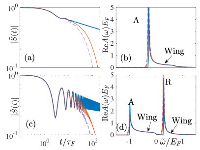
Figure 2: 1D Ramsey spectroscopy for (a) (b) attractive interaction $k_{F}a=-2$ and (c) (d) repulsive interaction $k_{F}a=2$. (a) and (c) show the overlap functions $\tilde{S}(t)$. (b) and (d) show the spectral functions ${\rm Re}A(\omega)$. Thick blue curves correspond to $k_{B}T^{\circ}=0$, thin red solid curves, and purple dashed curves correspond to $k_{B}T^{\circ}=0.03E_{F}$ and $k_{B}T^{\circ}=0.05E_{F}$, respectively.

In the previous section, we have given a general discussion of the underlying idea of 1D Ramsey responses of a heavy impurity and its relation to the absorption spectrum. Here, we show the detail of how to exactly solve the time-dependent problem nonperturbatively using the FDA. As a concrete example, we focus on the case where the background is a dilute single-component Fermi gas, which is considered to be noninteracting at ultracold temperature due to Pauli’s exclusion principle. As mentioned before, we assume only the background fermion only interacts with $|\uparrow\rangle$, which is dominated by the $s$-wave interaction that can be tuned via, e.g., Feshbach resonances. The corresponding Hamiltonian can be expressed in the form of Eq. 5, where

$$\mathcal{\hat{H}}_{\uparrow}=\mathcal{\hat{H}}_{\downarrow}+\sum_{\mathbf{k},\mathbf{q}}\tilde{V}(\mathbf{k}-\mathbf{q})\hat{c}_{\mathbf{k}}^{\dagger}\hat{c}_{\mathbf{q}}+\omega_{s},\ \mathcal{\hat{H}}_{\downarrow}=\sum_{\mathbf{k}}\epsilon_{\mathbf{k}}\hat{c}_{\mathbf{k}}^{\dagger}\hat{c}_{\mathbf{k}}.$$ (9)

Here, $\omega_{s}$ denotes the energy differences between the two spin levels. $\hat{c}_{\mathbf{k}}^{\dagger}$ and $\hat{c}_{\mathbf{k}}$ are creation and annihilation operators of the background fermions with momentum $\mathbf{k}$, respectively. $\epsilon_{\mathbf{k}}=k^{2}/2m$ is the single-particle kinetic energy of the background fermions with mass $m$. $\tilde{V}(\mathbf{k})$ is the Fourier transform of $V(\mathbf{r})$, the interaction potential between $|\uparrow\rangle$ and the background fermions. The low-temperature physics is determined by the $s$-wave energy-dependent scattering length $a(E_{F})=-\tan\eta(k_{F})/k_{F}$ at the Fermi energy $E_{F}=k_{F}^{2}/2m$, with $\eta(E_{F})$ being an energy-dependent $s$-wave scattering phase-shift obtained from a two-body scattering calculation with potential $V(\mathbf{r})$. For the simplicity of notation, we denote $a\equiv a(E_{F})$ hereafter.

For the example given here, we are interested in the so-called injection scheme where the spin is initially prepared in the noninteracting state $|\downarrow\rangle$. The initial density matrix of the system can therefore be written as $\rho_{i}=\rho_{{\rm FS}}\otimes|\downarrow\rangle\langle\downarrow|$, where the thermal density matrix of the background fermion at a finite temperature $T^{\circ}$ is given by

$$\rho_{{\rm FS}}=\prod_{\mathbf{k}}\left[n_{\mathbf{k}}\hat{c}_{\mathbf{k}}^{\dagger}\hat{c}_{\mathbf{k}}+\left(1-n_{\mathbf{k}}\right)\hat{c}_{\mathbf{k}}\hat{c}_{\mathbf{k}}^{\dagger}\right],$$ (10)

with the occupation of the momentum state

$$n_{\mathbf{k}}=\frac{1}{e^{\left(\epsilon_{\mathbf{k}}-\mu\right)/k_{B}T^{\circ}}+1}.$$ (11)

Here, $k_{B}$ is the Boltzman constant, $\mu\simeq E_{F}$ is the chemical potential determined by the number density of the background Fermi gas. We also define a diagonal matrix $\hat{n}$ with the matrix elements $n_{\mathbf{k}}$, which will become useful later.

For the simple 1D Ramsey spectrum, we apply a $\pi/2$ RF pulse at $t=0$ that can be described in the spin-basis as

$$\hat{R}_{-\hat{y}}\left(\frac{\pi}{2}\right)\equiv\left(\begin{array}[]{cc}R_{\uparrow\uparrow}^{(\pi/2)}\mathbf{1}&R_{\uparrow\downarrow}^{(\pi/2)}\mathbf{1}\\ R_{\downarrow\uparrow}^{(\pi/2)}\mathbf{1}&R_{\downarrow\downarrow}^{(\pi/2)}\mathbf{1}\end{array}\right)=\frac{1}{\sqrt{2}}\left(\begin{array}[]{cc}\mathbf{1}&\mathbf{1}\\ -\mathbf{1}&\mathbf{1}\end{array}\right),$$ (12)

where $\mathbf{1}$ represents the identity in the fermionic Hilbert space. For simplicity, we denote $\hat{\mathcal{R}}\equiv\hat{R}_{-\hat{y}}\left(\pi/2\right)$ hereafter. The total time evolution is determined by the unitary transformation

$$\hat{\mathcal{U}}(t)=\hat{U}(t)\hat{\mathcal{R}},$$ (13)

where

$$\hat{U}(t)=\left(\begin{array}[]{cc}e^{-i\mathcal{\hat{H}}_{\uparrow}t}&0\\ 0&e^{-i\mathcal{\hat{H}}_{\downarrow}t}\end{array}\right)$$ (14)

is the free time evolution operator in the spin basis representation after the RF pulse. The final state of the system is thus given by $\rho_{f}=\mathcal{U}\rho_{i}\mathcal{U}^{\dagger}$. Recall that $S(t)=\langle\sigma_{-}\rangle$, we arrive at

$$S(t)={\rm Tr}\left(\sigma_{-}\rho_{f}\right)={\rm Tr}\left(e^{i\hat{\mathcal{H}}_{\downarrow}t}e^{-i\mathcal{\hat{H}}_{\uparrow}t}\rho_{{\rm FS}}\right)$$ (15)

that reduces to Eq. (3) at zero temperature $k_{B}T^{\circ}=0$.

Since the complexity of the many-body Hamiltonians increases exponentially with the number of particles in the system, an exact calculation of $S(t)$ is usually inaccessible. However, in the case that $H_{\uparrow}$ and $H_{\downarrow}$ are both fermionic, bilinear many-body operators as in Eq. (9), the overlap function can reduce to a determinant in single-particle Hilbert space. This approach, namely FDA, is based on a mathematical trace formula that has been elegantly proved by Klich Klich (2003). (See Appendix A for details.) To proceed, we define $\hat{\mathcal{H}}_{\downarrow}\equiv\Gamma(h_{\downarrow})$ and $\hat{\mathcal{H}}_{\uparrow}\equiv\Gamma(h_{\uparrow})+\omega_{s}$. Here, $\Gamma(h)\equiv\sum_{\mathbf{k},\mathbf{q}}h_{\mathbf{k}\mathbf{q}}c_{\mathbf{k}}^{\dagger}c_{\mathbf{q}}$ is a bilinear fermionic many-body Hamiltonian in the Fock space, and $h_{\mathbf{k}\mathbf{q}}$ represents the matrix elements of the corresponding operator in the single-particle Hilbert space. Applying the Levitov’s formula, Eq. (58), gives $S(t)=e^{-i\omega_{s}t}\tilde{S}(t)$ where

$$\tilde{S}(t)={\rm det}[(\mathbf{1}-\hat{n})+R(t)\hat{n}],$$ (16)

and

$$R(t)=e^{ih_{\downarrow}t}e^{-ih_{\uparrow}t}.$$ (17)

Correspondingly, the frequency domain spectrum can be obtained by a Fourier transformation

$$A(\omega)=\frac{1}{\pi}\int_{0}^{\infty}e^{i\omega t}S(t)dt=\frac{1}{\pi}\int_{0}^{\infty}e^{i\tilde{\omega}t}\tilde{S}(t)dt.$$ (18)

Hereafter, unless specified otherwise, we denote $\tilde{\omega}=\omega-\omega_{s}$ for any frequency variable $\omega$. As one can see, $\omega_{s}$ has a simple effect as shifting the frequency origin of a 1D spectrum. Numerical calculations are carried out in a finite system confined in a sphere of radius $R$. Keeping the density constant, we increase $R$ towards infinity until numerical results are converged. Other details of numerical calculations are described in the Appendix.

Figures 2 (a) and (c) show $\tilde{S}(t)$ for attractive ($k_{F}a=-2$) and repulsive impurity interaction ($k_{F}a=+2$), respectively. The zero-temperature (solid blue curves) asymptotic behavior of the Ramsey response at $t\rightarrow\infty$ is given by

$$\tilde{S}(t)\simeq Ce^{-i\Delta Et}\left(\frac{1}{iE_{F}t+0^{+}}\right)^{\alpha}$$ (19)

$$+C_{b}e^{-i\left(\Delta E-E_{F}+E_{b}\right)t}\left(\frac{1}{iE_{F}t+0^{+}}\right)^{\alpha_{b}},$$

where $C$ and $C_{b}$ are both numerical constants independent with respect to $k_{F}a$ and $C_{b}=0$ for $a<0$. Here,

$$\alpha=\eta(E_{F})^{2}/\pi^{2}$$ (20)

and

$$\alpha_{b}=[1+\eta(E_{F})/\pi]^{2}$$ (21)

are determined by the $s$-wave scattering phase shifts $\eta(E_{F})$ at Fermi energy. $E_{b}$ is the binding energy of the shallowest bound state consisting of the impurity and a spin-up fermion for $a_{\uparrow}>0$ and $\Delta=0$. Furthermore, the change in energy can be understood as a renormalization of the Fermi sea by impurity scattering and is given by

$$\Delta E=\sum_{\nu=1}^{N}(E_{\nu}-\tilde{E}_{\nu}),$$ (22)

where $E_{\nu}$ and $\tilde{E}_{\nu}$ are the lowest $N$ eigenenergies of $\hat{h}_{\downarrow}$ and $\hat{h}_{\uparrow}$, respecitively, and the deeply bound states are excluded from $\tilde{E}_{\nu}$. Here $N$ is the number of particles fixed by the chemical potential $\mu$.

The corresponding spectral function ${\rm Re}A(\omega)$ is shown in Fig. 2 (b) and (d). The asymptotic behaviors of $\tilde{S}(t)$ translate into the threshold behaviors of spectra function at zero temperature. For frequency $\tilde{\omega}\approx\Delta E$, we have a singularity ${\rm Re}A(\omega)\propto\theta(\tilde{\omega}-\Delta E)|\tilde{\omega}-\Delta E|^{\alpha-1}$. If the impurity interaction is repulsive, an additional singularity shows up at $\tilde{\omega}\approx\omega_{b}=\Delta E-E_{F}+E_{b}$ as ${\rm Re}A(\omega)\propto\theta(\tilde{\omega}-\omega_{b})|\tilde{\omega}-\omega_{b}|^{\alpha_{b}-1}$. These singularities are called FES and are closely related to the polaron resonances (see Fig. 4 for example): the spectrum only shows one peak for attractive impurity interaction and shows two peaks for repulsive interaction. We, therefore, name the FESs in Fig. 2 (b) and (d) as attractive or repulsive singularities, denoted by “A” and “R”, respectively. However, different than the polaron peaks that are Dirac delta functions or Lorentzians, the FESs are power-law singularities, which is a manifestation of OC: the quasiparticle resonances are rendered into power-law singularities by the multiple particle-hole excitations near the surface of Fermi sea. At a finite temperature, however, the thermal fluctuation leads to an exponential decay $\tilde{S}(t)$ and Lorentzian-shape broadening of singularities in ${\rm Re}A(\omega)$, which allows FDA calculations to quantitatively predict the spectrum of mobile polaron if the thermal fluctuation is comparable to the recoil energy Cetina et al. (2016).

III A BCS superfliuid as a background medium

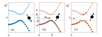
Figure 3: A sketch of the occupation and structure of the single-particle dispersion spectrum of a two-component superfluid Fermi gas with a positive chemical potential $\mu>0$ and the presence of a static impurity (black dot). (a) shows the spectrum when the impurity is in the noninteracting state (black arrow down) at zero temperature. When the impurity is in the interacting polaron state (black arrow up), the spectrum is shown in (b) at zero and (c) at finite temperature. Reprinted with permission from Wang et al. (2022a).

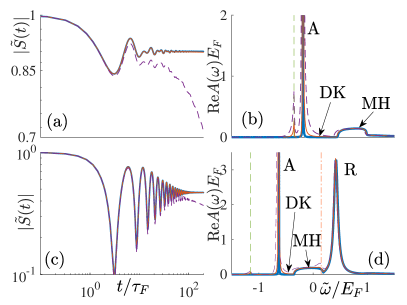
Figure 4: 1D Ramsey spectroscopy of magnetic impurity ($k_{F}a_{\Downarrow}=0$) in a BCS superfluid at the BCS side ($k_{F}a_{F}=-2$) for (a) (b) attractive impurity interaction $k_{F}a_{\Uparrow}=-2$ and (c) (d) repulsive impurity interaction $k_{F}a_{\Uparrow}=2$. (a) and (c) show the overlap functions $\tilde{S}(t)$. (b) and (d) show the spectral functions ${\rm Re}A(\omega)$. Thick blue curves correspond to $k_{B}T^{\circ}=0$, thin red solid curves, and purple dashed curves correspond to $k_{B}T^{\circ}=0.1E_{F}$ and $k_{B}T^{\circ}=0.15E_{F}$, respectively. A and R indicate the attractive and repulsive polaron resonances, respectively. DK and MH denote the dark continuum and molecule-hole continuum correspondingly. The green dashed, and purple dash-dotted lines indicate the YSR features $E_{{\rm RSR}}^{(-)}$ and $E_{{\rm RSR}}^{(+)}$, respectively.

This section extends the FDA to a strongly correlated superfluid background described by a standard BCS mean-field wavefunction Wang et al. (2022a, b). The purpose is twofold. First, we aim to construct an exactly solvable model for polaron with finite residue. This study shows that our system is suitable for an exact approach — an extended FDA. The presence of a pairing gap can efficiently suppress multiple particle-hole excitations and prevent Anderson’s OC. Therefore, our model provides a benchmark calculation of the polaron spectrum and rigorously examines all the speculated polaron features. We name our system “heavy crossover polaron” since the background Fermi gas can undergo a crossover from a Bose-Einstein condensation (BEC) to a BCS superfluid. Second, our prediction can be applied to investigate the background Fermi superfluid excitations, a long-standing topic in ultracold atoms. Polarons have already been realized in BEC and ideal Fermi gas experimentally, where the physics of these weakly interacting background gas is well understood. More recently, it has also been shown that polarons in BEC with a synthetic spin-orbit-coupling can reveal the nature of the background roton excitations (Wang et al., 2019). Investigating polaron physics in a strongly correlated Fermi superfluid at the BEC-BCS crossover, namely crossover polaron, has also been proposed in several pioneering works with approximated approaches Nishida (2015); Yi and Cui (2015); Pierce et al. (2019); Hu et al. (2022a); Bigué et al. (2022). Our exact method in the heavy impurity limit allows us to apply the polaron spectrum to measure the Fermi superfluid excitation features, such as the pairing gap and sub-gap Yu-Shiba-Rusinov (YSR) bound states (Yu, 1965; Shiba, 1968; Rusinov, 1969; Vernier et al., 2011; Jiang et al., 2011).

Our system consists of a localized impurity atom and a two-component Fermi superfluid with equal mass $m_{\Uparrow}=m_{\Downarrow}=m$. (Here, we use $|\Uparrow\rangle$ and $|\Downarrow\rangle$ to represent the two internal states of the background fermionic atoms, in contrast to the $|\uparrow\rangle$ and $|\downarrow\rangle$ for the impurity.) The interaction between unlike atoms in the two-component Fermi gas can be tuned by a broad Feshbach resonance and characterized by the $s$-wave scattering length $a_{F}$. At low temperatures $T$, these strongly interacting fermions undergo a crossover from a BEC to a BCS superfluid, which can be described by the celebrated BCS theory at a mean-field level. The full Hamiltonian can also be written in the form of Eq. 5, where $\mathcal{\hat{H}}_{\uparrow}=\mathcal{\hat{H}}_{\downarrow}+\omega_{s}+\hat{V}$,

$$\hat{V}=\sum_{\sigma=\Uparrow,\Downarrow}\sum_{\mathbf{k},\mathbf{q}}\tilde{V}_{\sigma}(\mathbf{k}-\mathbf{q})c_{\mathbf{k}\sigma}^{\dagger}c_{\mathbf{q}\sigma},$$ (23)

with $\tilde{V}_{\sigma}(\mathbf{k})$ being the Fourier transformation of the potential between impurity and $\sigma$-component fermion $V_{\sigma}(\mathbf{r})$, and

$$\mathcal{\hat{H}}_{\downarrow}=\hat{H}_{{\rm BCS}}\equiv K_{0}+\sum_{\mathbf{k}}\hat{\psi}_{\mathbf{k}}^{\dagger}\underline{h_{\downarrow}(\mathbf{k})}\hat{\psi}_{\mathbf{k}},$$ (24)

is the standard BCS Hamiltonian for noninteracting impurity. Here, $\hat{\psi}_{\mathbf{k}}^{\dagger}\equiv(c_{\mathbf{k}\Uparrow}^{\dagger},c_{-\mathbf{k}\Downarrow})$ is the Nambu spinor representation, with $c_{\mathbf{k}\Uparrow}^{\dagger}$ ($c_{\mathbf{k}\Downarrow}$) being the creation (annihilation) operator for a $\sigma$-component fermion with momentum $\mathbf{k}$. $K_{0}\equiv-\mathcal{V}\Delta^{2}/g+\sum_{\mathbf{k}}(\epsilon_{\mathbf{k}}-\mu)$, with $\mathcal{V}$ denoting the system volume and $\Delta$ being the pairing gap parameter. $\epsilon_{\mathbf{k}}\equiv\hbar^{2}k^{2}/2m$ is the single-particle dispersion relation, and $\mu$ is the chemical potential. We assume the populations of the two components are the same and fixed by $\mu$. The bare coupling constant $g$ should be renormalized by the $s$-wave scattering length $a_{F}$ between the two components via $g^{-1}=m/4\pi a_{F}-\sum_{\mathbf{k}}^{\Lambda}1/2\epsilon_{\mathbf{k}}$, where $\Lambda$ is an ultraviolet cut–off. $\underline{h_{\downarrow}(\mathbf{k})}$ can be regarded as a single-particle Hamiltonian $\hat{h}_{\downarrow}$ in momentum space and has a matrix form:

$$\underline{h_{\downarrow}(\mathbf{k})}=\left[\begin{array}[]{cc}\xi_{\mathbf{k}}&\Delta\\ \Delta&-\xi_{\mathbf{k}}\end{array}\right],$$ (25)

where $\xi_{\mathbf{k}}\equiv\epsilon_{\mathbf{k}}-\mu$. For a given scattering length $a_{F}$ and temperature $T^{\circ}$, $\Delta$ and $\mu$ are determined by a set of the mean-field number and gap equations Gurarie and Radzihovsky (2007).

To apply FDA, we need to express $\mathcal{H}_{\downarrow}$ and $\mathcal{H}_{\uparrow}$ in a bilinear form. It would be convenient to define $\hat{\psi}_{\mathbf{k}}^{\dagger}=(c_{\mathbf{k}\Uparrow}^{\dagger},c_{-\mathbf{k}\Downarrow})\equiv(c_{\mathbf{k}}^{\dagger},h_{\mathbf{k}}^{\dagger})$ and rewrite $\hat{V}$ as

$$\hat{V}=\sum_{\mathbf{k\mathbf{q}}}\left[\tilde{V}_{\Uparrow}(\mathbf{k}-\mathbf{q})c_{\mathbf{k}}^{\dagger}c_{\mathbf{q}}-\tilde{V}_{\Downarrow}(\mathbf{q}-\mathbf{k})h_{\mathbf{k}}^{\dagger}h_{\mathbf{q}}\right]+\sum_{\mathbf{k}}\tilde{V}_{\Downarrow}(0),$$ (26)

making the bilinear form apparent. We can also write the bilinear form of $\mathcal{\hat{H}}_{\uparrow}$ explicitly as

$$\hat{\mathcal{H}}_{\uparrow}=K_{0}+\omega_{0}+\omega_{s}+\sum_{\mathbf{k\mathbf{q}}}\hat{\psi}_{\mathbf{k}}^{\dagger}\underline{h_{\uparrow}(\mathbf{k},\mathbf{q})}\hat{\psi}_{\mathbf{q}},$$ (27)

where $\omega_{0}=\sum_{\mathbf{k}}\tilde{V}_{\Downarrow}(0)$ and

$$\underline{h_{\uparrow}(\mathbf{k},\mathbf{q})}=\underline{h_{\downarrow}(\mathbf{k})}\delta_{\mathbf{k}\mathbf{q}}+\left[\begin{array}[]{cc}\tilde{V}_{\Uparrow}(\mathbf{k}-\mathbf{q})&0\\ 0&-\tilde{V}_{\Downarrow}(\mathbf{q}-\mathbf{k})\end{array}\right]$$ (28)

can be regarded as a single-particle Hamiltonian $\hat{h}_{\uparrow}$ in momentum space and in a matrix form. We can see that, $\hat{h}_{\uparrow}$ and $\hat{h}_{\downarrow}$ are the single-particle representative of $\hat{\mathcal{H}}_{\uparrow}$ and $\hat{\mathcal{H}}_{\downarrow}$ up to some constants, respectively.

Diagonalizing $\underline{h_{\downarrow}(\mathbf{k})}$ gives the well-known BCS dispersion relation $E_{\nu}=\pm\mathcal{E}_{\mathbf{k}}=\pm\sqrt{\xi_{\mathbf{k}}^{2}+\Delta^{2}}$, where $\nu\equiv\{\pm,\mathbf{k}\}$ is a collective index. As sketched in Fig. 3 (a), this spectrum consists of positive and negative branches separated by an energy gap. Since we prepare the impurity initially in the noninteracting state, the atoms occupy the eigenstates of $\underline{h_{\downarrow}(\mathbf{k})}$ with a Fermi distribution $f(E_{\nu})=1/\left(e^{-E_{\nu}/k_{B}T}+1\right)$. At zero temperature, the many-body ground state can be regarded as a fully filled Fermi sea of the lower branch and a completely empty Fermi sea of the upper branch. When the impurity interaction is on, eigenvalues $\tilde{E}_{\nu}$ of $\underline{h_{\uparrow}(\mathbf{k})}$ still consists of two branches separated by the same gap, with each individual energy level shifted, as shown in Fig. 3 (b). Moreover, when the impurity scattering is magnetic ($a_{\Uparrow}\neq a_{\Downarrow})$, a sub-gap YSR bound state exists Yu (1965); Shiba (1968); Rusinov (1969); Vernier et al. (2011); Jiang et al. (2011).

It is worth noting that, in the many-body Hamiltonian $\hat{\mathcal{H}}_{\uparrow}$, we have assumed that the pairing order parameter $\Delta$ remains unchanged by introducing the interaction potential $V_{\sigma}(\mathbf{r})$. For a non-magnetic potential ($V_{\Uparrow}=V_{\Downarrow}$) that respects time-reversal symmetry, this is a reasonable assumption, according to Anderson’s theorem (Balatsky et al., 2006). For a magnetic potential ($V_{\Uparrow}\neq V_{\Downarrow}$), the local pairing gap near the impurity will be affected, as indicated by the presence of the YSR bound state. We will follow the typical non-self-consistent treatment of the magnetic potential in condensed matter physics (Balatsky et al., 2006; Yu, 1965) and assume a constant pairing gap as the first approximation for simplicity.

Inserting the bilinear forms of Hamiltonian into the expression of overlap function in Eq. (15) and applying FDA gives $S(t)=e^{-i\omega_{s}t}\tilde{S}(t)$ where

$$\tilde{S}(t)=e^{-i\omega_{0}t}{\rm det}[1-\hat{n}+e^{i\hat{h}_{\downarrow}t}e^{-i\hat{h}_{\uparrow}t}\hat{n}],$$ (29)

with $\hat{n}$ is the occupation number operator. The corresponding spectral function in the frequency domain is given by Eq. (18).

Figure 4 shows numerical results for a magnetic impurity ($k_{F}a_{\Downarrow}=0$) immersed in the background BCS superfluid at the BCS side ($k_{F}a_{F}=-2$). In sharp contrast to the noninteracting Fermi gases, for cases with a nonzero pairing gap, the asymptotic behavior in the long-time limit shows that $|\tilde{S}(t\rightarrow\infty)|\propto t^{0}$ approaches a constant. These asymptotic constants are larger for larger $\Delta$. Further details can be obtained by an asymptotic form that fits our numerical calculations perfectly

$$\tilde{S}(t)\simeq D_{a}e^{-iE_{a}t}+D_{r}e^{-iE_{r}t},$$ (30)

where $D_{r}=0$ for $a_{\uparrow}<0$. We obtain $D_{a}$, $D_{r}$, $E_{a}$ and $E_{r}$ from fitting and find that $E_{r}={\rm Re}E_{r}+i{\rm Im}E_{r}$ is, in general, complex. In contrast, $E_{a}=\sum_{E_{\nu}<0}(E_{\nu}-\tilde{E}_{\nu})$ (where $\tilde{E}_{\nu}$ excludes the two-body deeply bound states) is purely real and can be explained as a renormalization of the filled Fermi sea.

The long-time asymptotic behavior of $S(t)$ manifests itself as some characterized lineshape in the spectral function

$$A(\omega)\propto\begin{cases}Z_{a}\delta(\tilde{\omega}-E_{a})&\tilde{\omega}\approx E_{a}\\ Z_{r}\frac{\left|{\rm Im}E_{r}\right|/\pi}{(\tilde{\omega}-{\rm Re}E_{r})^{2}+({\rm Im}E_{r})^{2}}&\tilde{\omega}\approx{\rm Re}E_{r}\end{cases},$$ (31)

i.e., a $\delta$-function around $E_{a}$ and a Lorentzian around ${\rm Re}E_{r}$. The existence of the $\delta$-function peak unambiguously confirms the existence of a well-defined quasiparticle – the attractive polaron with energy $E_{a}$. The Lorentzian, on the other hand, can be recognized as a repulsive polaron with finite width and hence finite lifetime. Here, $Z_{a}=|D_{a}|$ and $Z_{r}=|D_{r}|$ are the residues of attractive and repulsive polaron, correspondingly. Numerically, we find that $Z_{a}\propto(\Delta/E_{F})^{\alpha_{a}}$ and $Z_{r}\propto(\Delta/E_{F})^{\alpha_{r}}$ at small $\Delta$. The existence of finite residue of polarons indicates that the pairing gap suppresses multiple particle-hole excitations and prevents OC, which eventually leads to the survival of well-defined polarons.

We also find that the attractive polaron separates from a molecule-hole continuum (denoted as MH in Fig. 4) by a region of anomalously low spectral weight, namely the “dark continuum” (denoted as DK in Fig. 4). The existence of a dark continuum has been previously observed in spectra of other polaron systems. However, most of these studies apply various approximations, and only recently, a diagrammatic Monte Carlo study proves the dark continuum is indeed physical (Goulko et al., 2016). Here, our FDA calculation of the heavy crossover polaron spectrum gives exact proof of the dark continuum. By comparing Fig. 4 and Fig. 2, we expect that the dark continuum vanishes in the $\Delta\rightarrow 0$ limit and the attractive polaron merges into the molecule-hole continuum, forming a power-law singularity with the “wing”. Similar behavior also can be observed for the repulsive polaron, where the associated molecule-hole continuum is much less significant and cannot be visually seen in Fig. 4.

Finite-temperature results are indicated by the thin red solid (purple dashed) curves for $k_{B}T=0.1E_{F}\ (0.15E_{F})$ in Fig. 4. Some surprising features show up, other than the expected thermal broadening. An enhancement of spectral weight appears sharply at the energy $E_{{\rm YSR}}^{(-)}=E_{a}-(\Delta-E_{{\rm YSR}})$ below the attractive polaron. This spectral feature corresponds to the decay process highlighted by the purple arrow in Fig. (c), where an additional particle initially excited to the upper Fermi sea by thermal fluctuation is driven to the YSR state. For the case of $k_{F}a_{\uparrow}>0$, a feature associated with the repulsive polaron appears at $E_{{\rm YSR}}^{(+)}={\rm Re}(E_{r})-(E_{{\rm YSR}}+\Delta)$, as indicated by the green arrow in Fig. 3 (c): an additional particle decays from the YSR state to the lower Fermi sea. The polaron spectrum can be applied to measure the superfluid gap $\Delta$ and $E_{{\rm YSR}}$. In particular, we notice, on the positive side $a_{\uparrow}>0$, if $E_{a}$, ${\rm Re}(E_{r})$, $E_{{\rm YSR}}^{(-)}$ and $E_{{\rm YSR}}^{(+)}$ can all be measured accurately, we have $2\Delta=E_{a}+{\rm Re}(E_{r})-E_{{\rm YSR}}^{(-)}-E_{{\rm YSR}}^{(+)}$ that does not depend on $E_{{\rm YSR}}$. Since this formula only relies on the existence of the gap and a mid-gap state, we anticipate it can be used to measure $\Delta$ accurately for a Fermi superfluid that can not be quantitatively described by the BCS theory.

IV Multidimension spectroscopy

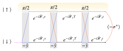
Figure 5: A sketch of EXSY (EXchange SpectroscopY) pulses scheme.

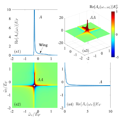
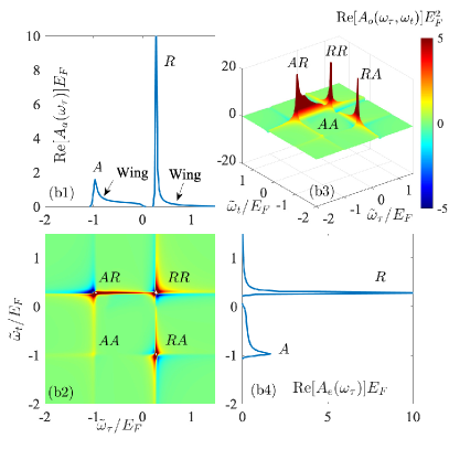
Figure 6: (a1) and (a4) shows the 1D absorption spectrum for attractive interaction $k_{F}a=-0.05$ and finite temperature $k_{B}T^{\circ}=0.03E_{F}$. The absorption singularity is denoted as $A$. (a2), and (a3) shows the contour, and 3D landscape of the 2D spin-echo spectrum ${\rm Re}[A_{o}(\omega_{\tau},\omega_{t})]$, where the diagonal peak is denoted as $AA$. (b1)-(b4) are the same as (a1)-(a4), correspondingly, but for repulsive interaction $k_{F}a=0.5$. There are two singularities in (b1), the absorption spectrum, namely repulsive and attractive singularities, which are denoted as $R$ and $A$. The corresponding diagonal peaks in (b2) and (b3) are denoted as $AA$ and $RR$, while the off-diagonal cross-peaks are denoted as $AR$ and $RA$. Reprinted with permission from Wang (2022)

In this section, we present another new extension of the FDA in the calculation of multidimensional (MD) Ramsey spectroscopy Wang (2022). Conventional Ramsey spectroscopy, such as the ones studied in previous sections, is called 1D since it shows the signal as a function of only one variable: the frequency of the single applied RF pulse or the time between the RF pulse and measurement. Here, we investigate a scenario where multiple RF pulses manipulate the impurity at several different times. The observed signal’s dependency on the time intervals between pulses or the corresponding Fourier transformation is called MD Ramsey spectroscopy.

Pushing 1D Ramsey spectroscopy to MD shares the same spirit as the widely successful MD nuclear magnetic resonance (NMR) and optical MD coherent spectroscopy (MDCS). MD spectroscopy not only improves the resolution and overcomes spectral congestion but also carries rich information on the correlations between resonance peaks and provides insights into physics that 1D spectroscopy cannot access. For example, in a 2D NMR spectroscopy, the peaks on the diagonal map the resonances in 1D spectroscopy; however, only coupled spins give rise to off-diagonal cross-peaks between corresponding resonances. The cross peaks are thus the signature of correlations between resonances, which the 1D spectrum cannot distinguish. In our system, the correlations in MD Ramsey spectroscopy are induced by the coupling between the spin and the background Fermi gas, a genuine many-body environment, and hence called many-body correlations.

We consider the same system described in Sec. II.2, a localized impurity immersed in a noninteracting Fermi gas but manipulated by multiple RF pulses. One example of a three-pulse scheme is shown in Fig. 5 (a), which is similar to one of the most common 2D NMR pulse sequences, namely EXSY (EXchange SpectroscopY). EXSY essentially measures the four-wave mixing response of our system. The time evolution is thus given by the unitary transformation

$$\mathcal{U}(t,T,\tau)=U(t)\mathcal{R}U(T)\mathcal{R}U(\tau)\mathcal{R}.$$ (32)

We define the MD responses as

$$S(\tau,T,t)=-{\rm Tr}(\sigma_{+}\rho_{f}),$$ (33)

where the choice of $\sigma_{+}$ and additional $-$1 prefactor are for conventions so that $S(\tau,T=0,t=0)$ is equivalent to the 1D overlap function $S(\tau)$. Notice that we have the relation $\mathcal{R}^{-1}\mathcal{R}^{-1}\mathcal{\mathcal{\sigma_{-}\mathcal{R\mathcal{R}}=-\sigma_{+}}}$.

The multidimensional response $S(\tau,T,t)$ can be written as a summation of sixteen contributions

$$S(\tau,T,t)=\sum_{i=1}^{16}S_{i}(\tau,T,t)\equiv\frac{1}{4}\sum_{i=1}^{16}\mathrm{Tr}[I_{i}(\tau,T,t)\rho_{{\rm FS}}],$$ (34)

where $I_{i}(\tau,T,t)$ are named pathways. These pathways are written as a direct product of six free-evolution operators $e^{-i\mathcal{\hat{H}^{\prime}}t^{\prime}}$ or their complex conjugates, such as Eqs. (36) and (37). Here, $\hat{\mathcal{H}}^{\prime}$ can be $\hat{\mathcal{H}}_{\uparrow}$ or $\hat{\mathcal{H}}_{\downarrow}$ and $t^{\prime}$ can be $\tau$, $T$, or $t$. The expressions of pathways are recognized to be similar to the optical paths in an interferometer as sketched in Fig. (5), where the free evolution-operator is illustrated by the solid black lines, the dashed lines in the grey beam splitter correspond to the matrix elements $R_{\sigma\sigma^{\prime}}^{(\pi/2)}$ of the rotating operator in the spin basis. The measurement operator $\sigma_{+}$ fixes the middle two terms that depend on $t$ as $...e^{i\hat{\mathcal{H}}_{\uparrow}t}e^{-i\mathcal{\hat{H}}_{\downarrow}t}...$, and the remaining operators each have two possibilities, leading to $2\times 4=16$ possible combinations.

A summation of the contributions of all sixteen pathways gives the total response $S(t,T,\tau)$, and the spectrum in the frequency domain can be obtained via a double Fourier transformation

$$A(\omega_{\tau},T,\omega_{t})=\frac{1}{\pi^{2}}\int_{0}^{\infty}\int_{0}^{\infty}dtd\tau e^{i\omega_{\tau}\tau}S(\tau,T,t)e^{-i\omega_{t}t},$$ (35)

where $\omega_{t}$ and $\omega_{\tau}$ are interpreted as an absorption and emission frequency, respectively. On the other hand, the dependence of $A(\omega_{\tau},T,\omega_{t})$ on the mixing time $T$ can reveal the many-body coherent and incoherent dynamics Tempelaar and Berkelbach (2019). The physical process underlying $A(\omega_{\tau},T,\omega_{t})$ can be interpreted as an inequilibrium dynamical evolution: the system first gets excited by absorbing a photon with frequency $\omega_{\tau}$, after a period of mixing time $T$, and then emits a photon with frequency $\omega_{t}$. We notice that $A(\omega_{\tau},T,\omega_{t})=\sum_{i=1}^{16}A_{i}(\omega_{\tau},T,\omega_{t})$ can also be expressed as a summation of sixteen pathways, where the expression of each pathway is given by Eq. (35), with $A$ and $S$ replaced by $A_{i}$ and $S_{i}$, respectively.

We can take the rotating wave approximation and consider only two dominant pathways (with details given by Wang (2022))

$$I_{1}(\tau,T,t)=e^{i\hat{\mathcal{H}}_{\downarrow}\tau}e^{i\hat{\mathcal{H}}_{\uparrow}T}e^{i\hat{\mathcal{H}}_{\uparrow}t}e^{-i\hat{\mathcal{H}}_{\downarrow}t}e^{-i\hat{\mathcal{H}}_{\uparrow}T}e^{-i\hat{\mathcal{H}}_{\uparrow}\tau},$$ (36)

$$I_{2}(\tau,T,t)=e^{i\hat{\mathcal{H}}_{\downarrow}\tau}e^{i\hat{\mathcal{H}}_{\downarrow}T}e^{i\hat{\mathcal{H}}_{\uparrow}t}e^{-i\hat{\mathcal{H}}_{\downarrow}t}e^{-i\hat{\mathcal{H}}_{\downarrow}T}e^{-i\hat{\mathcal{H}}_{\uparrow}\tau}.$$ (37)

It should be notice that the expression of $I_{1}(\tau,T,t)$ and $I_{2}(\tau,T,t)$ are similar to those correspond to the excited state emision (ESE) and ground state breaching (GSB) in the rephasing 2D coherent spectra Hu et al. (2022b).

The contribution of each pathway, $S_{i}(\tau,T,t)$, can be calculated exactly via FDA. To proceed, we define $\mathcal{H}_{\downarrow}\equiv\Gamma(h_{\downarrow})$ and $\mathcal{H}_{\uparrow}\equiv\Gamma(h_{\uparrow})+\omega_{s}$. Here $\Gamma(h)\equiv\sum_{\mathbf{k},\mathbf{q}}h_{\mathbf{k}\mathbf{q}}c_{\mathbf{k}}^{\dagger}c_{\mathbf{q}}$ is a bilinear fermionic many-body Hamiltonian in the Fock space, and $h_{\mathbf{k}\mathbf{q}}$ represents the matrix elements of the corresponding operator in the single-particle Hilbert space. These matrix elements are explicitly given by $(h_{\downarrow})_{\mathbf{k}\mathbf{q}}=\epsilon_{\mathbf{k}}\delta_{\mathbf{k}\mathbf{q}}$ and $(h_{\uparrow})_{\mathbf{k}\mathbf{q}}=\epsilon_{\mathbf{k}}\delta_{\mathbf{k}\mathbf{q}}+\tilde{V}(\mathbf{k}-\mathbf{q})$. With these definitions, we can rewrite

$$S_{i}(\tau,T,t)=\frac{1}{4}\tilde{S}_{i}(\tau,T,t)e^{-i\omega_{s}f_{i}(t,T,\tau)},$$ (38)

where $e^{-i\omega_{s}f_{i}(t,T,\tau)}$ gives a simple phase and $\tilde{S}_{i}(\tau,T,t)$ is a product of the exponentials of the bilinear fermionic operator, both of which can be calculated exactly. For example, we have $S_{1}(\tau,T,t)=\tilde{S}_{1}(\tau,T,t)e^{i\omega_{s}t}e^{-i\omega_{s}\tau}/4$, where

$$\begin{aligned} \tilde{S}_{1}(\tau,T,t)=&{\rm Tr}[e^{i\Gamma(h_{\downarrow})\tau}e^{i\Gamma(h_{\uparrow})T}e^{i\Gamma(h_{\uparrow})t}\times\\ &e^{-i\Gamma(h_{\downarrow})t}e^{-i\Gamma(h_{\uparrow})T}e^{-i\Gamma(h_{\uparrow})\tau}\rho_{{\rm FS}}]\end{aligned}.$$ (39)

Applying Levitov’s formula Klich (2003); Wang et al. (2022a, b) gives

$$\tilde{S}_{1}(\tau,T,t)={\rm det}[(1-\hat{n})+R_{1}(\tau,T,t)\hat{n}],$$ (40)

with

$$R_{1}(\tau,T,t)=e^{ih_{\downarrow}\tau}e^{ih_{\uparrow}T}e^{ih_{\uparrow}t}e^{-ih_{\downarrow}t}e^{-ih_{\uparrow}T}e^{-ih_{\uparrow}\tau},$$ (41)

and $\hat{n}=n_{\mathbf{k}}\delta_{\mathbf{k}\mathbf{k}^{\prime}}$, where $n_{\mathbf{k}}=1/(e^{\epsilon_{\mathbf{k}}/k_{B}T^{\circ}}+1)$ denotes the single-particle occupation number operator.

The 2D spectrum $A_{o}(\omega_{\tau},\omega_{t})\equiv A(\omega_{\tau},T=0,\omega_{t})$ in Figs. 6 (a2) and (a3) shows a double dispersion lineshape commonly found in 2D NMR around $(\tilde{\omega}_{\tau},\tilde{\omega}_{t})\approx(\tilde{\omega}_{A-},\tilde{\omega}_{A-})$, which is called a diagonal peak denoted as $AA$. For attractive interaction $k_{F}a=-0.5$, the attractive singularity appears at $\tilde{\omega}_{A-}\approx-0.28E_{F}$ in the absorption spectrum. We have numerically verified that the integration of 2D spectroscopy over emission frequency $\omega_{t}$ gives the 1D absorption spectrum $A_{a}(\omega_{\tau})$ (not shown here). Interestingly, we can observe that there is no diagonal spectral weight corresponding to the wing. Rather, the spectral weight on the off-diagonal $A_{o}(\omega_{\tau},\omega_{t}\approx\omega_{A-})$ and $A_{o}(\omega_{\tau}\approx\omega_{A-},\omega_{t})$ is significant and resembles the lineshape of the wing. This is a non-trivial manifestation of OC in the 2D spectroscopy: the inhomogeneous and homogeneous lineshape does not have the OC characteristic, i.e., a power-law singularity and a broad lineshape that resembles the wings in the 1D spectroscopy Knap et al. (2012). Here, the inhomogeneous and homogeneous lineshape refer to the lineshape near a singularity along the diagonal or the direction perpendicular to the diagonal. As we can observe, the widths of the singularity are much sharper along these two directions, which might help experimental identification of the singularity, especially at finite temperatures. The homogeneous and inhomogeneous broadenings in MD spectroscopy also have their own experimental significance, similar to their NMR or optical counterpart. In a realistic experiment, the ensemble average of the impurity signal can give rise to a further inhomogeneous broadening induced by the disorder of the local environment (such as spatial magnetic field fluctuation). However, these disorders are usually non-correlated and would not introduce homogeneous broadening Nardin et al. (2015); Hao et al. (2016, 2017).

For repulsive interaction $k_{F}a=0.5$, there are two singularities, the attractive and repulsive singularities, in the 1D absorption spectrum. These singularities appear at $\tilde{\omega}_{A+}\approx-0.98E_{F}$ and $\tilde{\omega}_{R+}\approx 0.28E_{F}$ in Figs. 6 (b1) and (b4). As shown in Fig. 6 (b2) and (b3), there are two diagonal peaks, $AA$ and $RR$, in the 2D spectroscopy that mirror the attractive and repulsive singularities. In addition, there are also two significant cross-peaks denoted as $AR$ and $RA$. The physical interpretations of cross peaks are similar to those observed in 2D NMR, where strong cross-peaks between the two spin resonances indicate strong coupling between the two spins. In our system, the correlation between attractive and repulsive singularities is induced by the coupling between spin and the background Fermi gas, a many-body environment, which is named a many-body quantum correlation. The strong off-diagonal peaks, therefore, indicate a strong many-body quantum correlation between the attractive and repulsive singularity induced by the many-body environment. As far as we know, this is the first prediction of many-body correlations between Fermi edge singularities in cold atom systems. If the impurity has a finite mass or the background Fermi gas is replaced by a superfluid with an excitation gap, we expect these cross-peaks would remain and represent the correlations between attractive and repulsive polarons Wang et al. (2022a, b). The method reviewed here can also be straightforwardly applied to calculate the coherent and relaxation dynamics of the system in terms of the mixing-time $T$ dependence of the MD Ramsey spectroscopy Wang (2022). We also remark here that a calculation of the MD Ramsey spectroscopy for a finite mass impurity has recently been developed using a Chevy’s ansatz approximation method Wang et al. (2022c).

Appendix A Klich’s proof of a trace formula

One of the key equations in the functional determinant approach formalism is a trace formula

$${\rm Tr}\left[e^{\Gamma(A_{1})}e^{\Gamma(A_{2})}...e^{\Gamma(A_{N})}\right]={\rm det}\left(\mathbf{1}-\xi e^{A_{1}}e^{A_{2}}...e^{A_{N}}\right)^{-\xi},$$ (42)

where $\mathbf{1}$ is an identity matrix of the dimension of single-particle Hilbert space, $\xi=1$ for bosons and $\xi=-1$ for fermions. Here the many-body Fock space operator

$$\Gamma(A_{n})=\sum_{ij}\langle i|A_{n}|j\rangle a_{i}^{\dagger}a_{j}$$ (43)

is the second quantized version of a single particle operator $A_{n}$, and $n\in\{1,2,...,N\}$ are integer subscripts. In contrast, $A_{n}$ is defined as an operator on the single particle Hilbert space, with matrix elements $\langle i|A_{n}|j\rangle$, where $|i\rangle$ are single-particle basis corresponding to the creation operator $a_{i}^{\dagger}$. Here, we included the proof for completeness, mainly following Klich’s elegant proof Klich (2003).

First, we prove for a single operator, ${\rm Tr}\left[e^{\Gamma(A_{1})}\right]={\rm det}\left(\mathbf{1}-\xi e^{A_{1}}\right)^{-\xi}$. We recall that any matrix $A_{1}$ can be written in a basis (corresponding to creation operator $b_{i}^{\dagger}$) which it is of the form $D+K$, where $D$ is a diagonal matrix with elements $D_{\nu\nu}\equiv\lambda_{\nu}$ known as eigenvalues of the matrix and $K$ is an upper triangular. Since the upper trangular $K$ does not contribute to the trace, we have

$${\rm Tr}\left[e^{\Gamma(A_{1})}\right]={\rm Tr}\left[e^{\Gamma(D)}\right]={\rm Tr}\left[\prod_{\nu=1}^{K}e^{\lambda_{\nu}b_{\nu}^{\dagger}b_{\nu}}\right].$$ (44)

Notice that the trace is taking over the Fock space basis $|\vec{\alpha}\rangle\equiv|\alpha_{1}\alpha_{2}...\alpha_{K}\rangle$ with $\alpha_{\nu}$ being the occupation number of the single-particle basis $|\nu\rangle$ corresponding to $b_{\nu}^{\dagger}$. For fermions, $\vec{\alpha}$ are vectors of zeros and ones and for bosons vectors with integer coefficients. In such occupation number representation, the trace can be expressed as

$${\rm Tr}\left[\prod_{\nu=1}^{K}e^{\lambda_{\nu}b_{\nu}^{\dagger}b_{\nu}}\right]=\prod_{\nu=1}^{K}\sum_{\alpha_{\nu}}e^{\lambda_{\nu}\alpha_{\nu}},$$ (45)

where

$$\sum_{\alpha_{\nu}}e^{\lambda_{\nu}\alpha_{\nu}}=(1-\xi e^{\lambda_{\nu}})^{-\xi}=\begin{cases}1+e^{\lambda_{\nu}},\ ,\xi=-1&{\rm Fermion},\\ 1/(1-e^{\lambda_{\nu}}),\ \xi=1&{\rm Boson}.\end{cases}$$ (46)

The fact that $\lambda_{\nu}$ are eigenvalues of $A_{1}$, which implies $(1-\xi e^{\lambda_{\nu}})^{-\xi}$ are eigenvalues of $(1-\xi e^{A_{1}})^{-\xi}$, leads to the products of eigenvalues $\prod_{\nu=1}^{K}(1-\xi e^{\lambda_{\nu}})^{-\xi}={\rm det}(\mathbf{1}-\xi e^{A_{1}})^{-\xi}$. Consequently, we prove

$${\rm Tr}\left[e^{\Gamma(A_{1})}\right]={\rm det}\left(\mathbf{1}-\xi e^{A_{1}}\right)^{-\xi}$$ (47)

as promised. We remark that this formula does not depend on the single-state basis, and an intuitive way of understanding this formula can be thinking of ${\rm Tr}\left[e^{\Gamma(A_{1})}\right]$ as the partition function of a system with Hamiltonian $-A_{1}$ at temperature $k_{B}T^{\circ}=1$.

We proceed to prove the formula for the product of two operators

$${\rm Tr}\left[e^{\Gamma(A_{1})}e^{\Gamma(A_{2})}\right]={\rm det}\left(\mathbf{1}-\xi e^{A_{1}}e^{A_{2}}\right)^{-\xi}.$$ (48)

One can show that, the Fock space operators $\Gamma(A_{n})$ in Eq. (43) satisfies

$$[\Gamma(A_{n}),\Gamma(A_{m})]=\Gamma([A_{n},A_{m}]),$$ (49)

which implies for an $N$ dimensional single particle Hilbert space $\Gamma$ is a representation of the usual Lie algebra of matrices $gl(N)$. As a result, the Baker-Campbell-Hausdorf formula

$$e^{A_{1}}e^{A_{2}}=e^{B}$$ (50)

leads to

$$e^{\Gamma(A_{1})}e^{\Gamma(A_{2})}=e^{\Gamma(B)}.$$ (51)

Therefore, we have ${\rm Tr}\left[e^{\Gamma(A_{1})}e^{\Gamma(A_{2})}\right]={\rm Tr}[e^{\Gamma(B)}]={\rm det}\left(\mathbf{1}-\xi e^{B}\right)^{-\xi}={\rm det}\left(\mathbf{1}-\xi e^{A_{1}A_{2}}\right)^{-\xi}$ as shown in Eq. (48). One can also see that this relation can immediately be generalized in the same way to products of more then two operators as our trace formula Eq. (42).

A pedagogical example is the dimension of the Fock space whose coresponding single particle Hilbert space has a dimension of $N$, which is given by

$${\rm Tr}\mathbf{1}={\rm Tr}e^{\Gamma(0)}={\rm det}(1-\xi)^{-\xi}=\begin{cases}2^{N}&{\rm Fermions}\\ \infty&{\rm Bosons}\end{cases},$$ (52)

as it should be.

In this review, a commonly encounter case is that the last operator $e^{\Gamma(A_{N})}$ in the trace formula is a fermion density matrix in a bilinear form

$$\rho_{F} =\frac{1}{Z}\exp\left(-\sum_{\alpha}\lambda_{\alpha}\hat{a}_{\alpha}^{\dagger}\hat{a}_{\alpha}\right),$$ (53)

$$\equiv\prod_{\alpha}\left[n_{\alpha}\hat{a}_{\alpha}^{\dagger}\hat{a}_{\alpha}+\left(1-n_{\alpha}\right)\hat{a}_{\alpha}\hat{a}_{\alpha}^{\dagger}\right],$$

where

$$e^{-\lambda_{\alpha}}=\frac{n_{\alpha}}{1-n_{\alpha}},$$ (54)

with $n_{\alpha}$ being the distribution of fermions in the single particle state corresponding to $\hat{a}_{\alpha}^{\dagger}$. The normalized constant is given by $Z={\rm Tr}\exp\left(-\sum_{\alpha}\lambda_{\alpha}\hat{a}_{\alpha}^{\dagger}\hat{a}_{\alpha}\right)={\rm det}[\left(1-\hat{n}\right)^{-1}]$, where $\hat{n}$ is a diagonal matrix with matrix elements $n_{\alpha}$.

One familiar example is the non-interacting Fermions at a the finite temperature, where $\hat{a}_{\alpha}^{\dagger}$ creates a fermion in the state with single-particle energy $\epsilon_{\alpha}$ and

$$n_{\alpha}=\frac{1}{e^{\left(\epsilon_{\alpha}-\mu\right)/k_{B}T^{\circ}}+1},\ \lambda_{\alpha}=\frac{\epsilon_{\alpha}-\mu}{k_{B}T^{\circ}}.$$ (55)

Here, $\mu$ is the chemical potential, and $k_{B}$ is the Boltzmann constant.

In this case, we have

$${\rm Tr}\left[e^{\Gamma(A_{1})}e^{\Gamma(A_{2})}...e^{\Gamma(A_{N-1})}\rho_{F}\right]= \frac{1}{Z}{\rm det}[\mathbf{1}+e^{A_{1}}e^{A_{2}}...$$ (56)

$$\times e^{A_{N-1}}e^{-\underline{\lambda}}]$$

where in the basis of single particle states corresponding to $a_{\alpha}^{\dagger}$, $e^{-\underline{\lambda}}$ is a diagonal matrix with matrix elements $e^{-\lambda_{\alpha}}$, which leads to

$$e^{-\underline{\lambda}}=\hat{n}\left(\mathbf{1}-\hat{n}\right)^{-1}.$$ (57)

Inserting the expression of $e^{-\underline{\lambda}}$ and $Z$ in terms of distribution matrix $\hat{n}$ gives

$${\rm Tr}\left[e^{\Gamma(A_{1})}e^{\Gamma(A_{2})}...e^{\Gamma(A_{N-1})}\rho_{F}\right]=\det[(\mathbf{1}-\hat{n})+\hat{R}\hat{n}],$$ (58)

where

$$\hat{R}=e^{A_{1}}e^{A_{2}}...e^{A_{N-1}}.$$ (59)

Another closely related and useful trace formula is

$${\rm Tr}\left[e^{\Gamma(A_{1})}e^{\Gamma(A_{2})}...e^{\Gamma(A_{N})}a_{i}^{\dagger}a_{j}\right]= (\mathbf{1}-\xi e^{-W})_{ji}^{-1}$$ (60)

$$\times{\rm det}\left(\mathbf{1}-\xi e^{W}\right)^{-\xi}$$

where $e^{W}=e^{A_{1}}e^{A_{2}}...e^{A_{N}}$. Noticing that ${\rm Tr}\left[e^{\Gamma(A_{1})}e^{\Gamma(A_{2})}...e^{\Gamma(A_{N})}\right]={\rm Tr}[e^{\Gamma(W)}]$ leads to

$${\rm Tr}\left[e^{\Gamma(A_{1})}e^{\Gamma(A_{2})}...e^{\Gamma(A_{N})}a_{i}^{\dagger}a_{j}\right]=\frac{\partial}{\partial W_{ij}}{\rm Tr}[e^{\Gamma(W)}],$$ (61)

where $W_{ij}\equiv\langle i|W|j\rangle$ are the matrix element of $W$. Applying Jacobi’s formula gives

$$\frac{\partial{\rm det}(\mathbf{1}-\xi e^{W})^{-\xi}}{\partial W_{ij}}={\rm{\rm det}}(\mathbf{1}-\xi e^{W})^{-\xi}{\rm Tr}[(\mathbf{1}-\xi e^{-W})^{-1}\frac{\partial W}{\partial W_{ij}}],$$ (62)

where taking the trace on the right-hand-side gives ${\rm Tr}[(\mathbf{1}-\xi e^{-W})^{-1}\partial W/\partial W_{ij}]=(\mathbf{1}-\xi e^{-W})_{ji}^{-1}$, which evntually leads to Eq. (60).

Appendix B Numerical Calculations

Numerical calculations are carried out in a finite system confined in a sphere of radius $R$. Keeping the density constant, we increase $R$ towards infinity until numerical results are converged. Typically, we choose $k_{F}R=250\pi$ in a calculation. We focus on the $s$-wave interaction channel between $|\uparrow\rangle$ and the background fermions near a broad Feshbach resonance, which can be well mimicked by a spherically symmetric and short-range van-der-Waals type potential $V(r)=-C_{6}\exp(-r_{0}^{6}/r^{6})/r^{6}$ Wang et al. (2012a, b, c). Here, $C_{6}$ determines the van-der-Waals length $l_{{\rm vdW}}=(2mC_{6})^{1/4}/2$, and we choose $l_{{\rm vdW}}k_{F}=0.01\ll 1$, so the short-range details are unimportant. $r_{0}$ is the short-range parameter that tunes the scattering length $a$. We choose $k_{F}r_{0}\approx 7\times 10^{-3}$, which can support two bound states on the positive side. We also include about $1100$ continuum states in a typical calculation. Covergence with respect to both number of bound states and continnum states have been tested.

References

- Mahan (2000) Gerald D. Mahan, Many Particle Physics, 3rd ed. (Kluwer, New York, 2000).
- Mahan (1967a) G. D. Mahan, “Excitons in degenerate semiconductors,” Phys. Rev. 153, 882–889 (1967a).
- Mahan (1967b) G. D. Mahan, “Excitons in metals: Infinite hole mass,” Phys. Rev. 163, 612–617 (1967b).
- Nozières and De Dominics (1969) P. Nozières and C. T. De Dominics, “Singularities in the x-ray absorption and emission of metals. iii. one-body theory exact solution,” Phys. Rev. 178, 1097–1107 (1969).
- Anderson (1967) P. W. Anderson, “Infrared catastrophe in fermi gases with local scattering potentials,” Phys. Rev. Lett. 18, 1049–1051 (1967).
- Matveev and Larkin (1992) K. A. Matveev and A. I. Larkin, “Interaction-induced threshold singularities in tunneling via localized levels,” Phys. Rev. B 46, 15337–15347 (1992).
- Geim et al. (1994) A. K. Geim, P. C. Main, N. La Scala, L. Eaves, T. J. Foster, P. H. Beton, J. W. Sakai, F. W. Sheard, M. Henini, G. Hill, and M. A. Pate, “Fermi-edge singularity in resonant tunneling,” Phys. Rev. Lett. 72, 2061–2064 (1994).
- Ogawa et al. (1992) Tetsuo Ogawa, Akira Furusaki, and Naoto Nagaosa, “Fermi-edge singularity in one-dimensional systems,” Phys. Rev. Lett. 68, 3638–3641 (1992).
- Prokof’ev (1994) N. V. Prokof’ev, “Fermi-edge singularity with backscattering in the luttinger-liquid model,” Phys. Rev. B 49, 2148–2151 (1994).
- Komnik et al. (1997) Andrei Komnik, Reinhold Egger, and Alexander O. Gogolin, “Exact fermi-edge singularity exponent in a luttinger liquid,” Phys. Rev. B 56, 1153–1160 (1997).
- Bascones et al. (2000) E. Bascones, C. P. Herrero, F. Guinea, and Gerd Schön, “Nonequilibrium effects in transport through quantum dots,” Phys. Rev. B 61, 16778–16786 (2000).
- Levitov and Lee (1996) Leonid S. Levitov and Hyunwoo Lee, “Electron counting statistics and coherent states of electric current,” J. Math. Phys. 37, 4845 (1996).
- Klich (2003) I. Klich, Full Counting Statistics: an Elementary Derivation of Levitov’s Formula (Kluwer, Dordrecht, 2003).
- Schönhammer (2007) K. Schönhammer, “Full counting statistics for noninteracting fermions: Exact results and the Levitov-Lesovik formula,” Phys. Rev. B 75, 205329 (2007).
- Ivanov and Abanov (2013) Dmitri A Ivanov and Alexander G Abanov, “Fisher-Hartwig expansion for Toeplitz determinants and the spectrum of a single-particle reduced density matrix for one-dimensional free fermions,” J. Phys. A: Math. Theor. 46, 375005 (2013).
- Muzykantskii et al. (2003) B. Muzykantskii, N. d’Ambrumenil, and B. Braunecker, “Fermi-edge singularity in a nonequilibrium system,” Phys. Rev. Lett. 91, 266602 (2003).
- d’Ambrumenil and Muzykantskii (2005) N. d’Ambrumenil and B. Muzykantskii, “Fermi gas response to time-dependent perturbations,” Phys. Rev. B 71, 045326 (2005).
- Abanin and Levitov (2005) D. A. Abanin and L. S. Levitov, “Fermi-edge resonance and tunneling in nonequilibrium electron gas,” Phys. Rev. Lett. 94, 186803 (2005).
- Abanin and Levitov (2004) D. A. Abanin and L. S. Levitov, “Tunable fermi-edge resonance in an open quantum dot,” Phys. Rev. Lett. 93, 126802 (2004).
- Chang and Reichman (2019) Yao-Wen Chang and David R. Reichman, “Many-body theory of optical absorption in doped two-dimensional semiconductors,” Phys. Rev. B 99, 125421 (2019).
- (21) Lachlan P Lindoy, Yao-Wen Chang, and David R Reichman, “Two-dimensional spectroscopy of two-dimensional materials,” arXiv:2206.01799 (2022).
- Knap et al. (2012) Michael Knap, Aditya Shashi, Yusuke Nishida, Adilet Imambekov, Dmitry A. Abanin, and Eugene Demler, “Time-dependent impurity in ultracold fermions: Orthogonality catastrophe and beyond,” Phys. Rev. X 2, 041020 (2012).
- Schmidt et al. (2018a) R. Schmidt, M. Knap, D. A. Ivanov, J.-S. You, M. Cetina, and E. Demler, “Universal many-body response of heavy impurities coupled to a Fermi sea: a review of recent progress,” Rep. Prog. Phys. 81, 024401 (2018a).
- Goold et al. (2011) J. Goold, T. Fogarty, N. Lo Gullo, M. Paternostro, and Th. Busch, “Orthogonality catastrophe as a consequence of qubit embedding in an ultracold fermi gas,” Phys. Rev. A 84, 063632 (2011).
- Chevy (2006) F. Chevy, “Universal phase diagram of a strongly interacting Fermi gas with unbalanced spin populations,” Phys. Rev. A 74, 063628 (2006).
- Combescot et al. (2007) R. Combescot, A. Recati, C. Lobo, and F. Chevy, “Normal state of highly polarized Fermi gases: Simple many-body approaches,” Phys. Rev. Lett. 98, 180402 (2007).
- Punk et al. (2009) M. Punk, P. T. Dumitrescu, and W. Zwerger, “Polaron-to-molecule transition in a strongly imbalanced Fermi gas,” Phys. Rev. A 80, 053605 (2009).
- Cui and Zhai (2010) Xiaoling Cui and Hui Zhai, “Stability of a fully magnetized ferromagnetic state in repulsively interacting ultracold Fermi gases,” Phys. Rev. A 81, 041602 (2010).
- Mathy et al. (2011) Charles J. M. Mathy, Meera M. Parish, and David A. Huse, “Trimers, molecules, and polarons in mass-imbalanced atomic Fermi gases,” Phys. Rev. Lett. 106, 166404 (2011).
- Schmidt et al. (2012) Richard Schmidt, Tilman Enss, Ville Pietilä, and Eugene Demler, “Fermi polarons in two dimensions,” Phys. Rev. A 85, 021602 (2012).
- Parish and Levinsen (2013) Meera M. Parish and Jesper Levinsen, “Highly polarized fermi gases in two dimensions,” Phys. Rev. A 87, 033616 (2013).
- Levinsen et al. (2015) Jesper Levinsen, Meera M. Parish, and Georg M. Bruun, “Impurity in a bose-einstein condensate and the efimov effect,” Phys. Rev. Lett. 115, 125302 (2015).
- Hu et al. (2016) Hui Hu, An-Bang Wang, Su Yi, and Xia-Ji Liu, “Fermi polaron in a one-dimensional quasiperiodic optical lattice: The simplest many-body localization challenge,” Phys. Rev. A 93, 053601 (2016).
- Hu et al. (2018) Hui Hu, Brendan C. Mulkerin, Jia Wang, and Xia-Ji Liu, “Attractive fermi polarons at nonzero temperatures with a finite impurity concentration,” Phys. Rev. A 98, 013626 (2018).
- Mulkerin et al. (2019) B. C. Mulkerin, X.-J. Liu, and H. Hu, “Breakdown of the fermi polaron description near fermi degeneracy at unitarity,” Ann. Phys. (NY) 407, 29 (2019).
- Parish et al. (2021) Meera M. Parish, Haydn S. Adlong, Weizhe Edward Liu, and Jesper Levinsen, “Thermodynamic signatures of the polaron-molecule transition in a fermi gas,” Phys. Rev. A 103, 023312 (2021).
- Lobo et al. (2006) C. Lobo, A. Recati, S. Giorgini, and S. Stringari, “Normal state of a polarized Fermi gas at unitarity,” Phys. Rev. Lett. 97, 200403 (2006).
- Kroiss and Pollet (2015) Peter Kroiss and Lode Pollet, “Diagrammatic monte carlo study of a mass-imbalanced fermi-polaron system,” Phys. Rev. B 91, 144507 (2015).
- Goulko et al. (2016) Olga Goulko, Andrey S. Mishchenko, Nikolay Prokof’ev, and Boris Svistunov, “Dark continuum in the spectral function of the resonant fermi polaron,” Phys. Rev. A 94, 051605 (2016).
- Pessoa et al. (2021) Renato Pessoa, S. A. Vitiello, and L. A. Peña Ardila, “Finite-range effects in the unitary fermi polaron,” Phys. Rev. A 104, 043313 (2021).
- Cetina et al. (2016) M. Cetina, M. Jag, R. S. Lous, I. Fritsche, J. T. M.Walraven, R. Grimm, J. Levinsen, M. M. Parish, R. Schmidt, M. Knap, and E. Demler, “Ultrafast many-body interferometry of impurities coupled to a fermi sea,” Science 354, 96 (2016).
- Liu et al. (2019) Weizhe Edward Liu, Jesper Levinsen, and Meera M. Parish, “Variational approach for impurity dynamics at finite temperature,” Phys. Rev. Lett. 122, 205301 (2019).
- You et al. (2019) Jhih-Shih You, Richard Schmidt, Dmitri A. Ivanov, Michael Knap, and Eugene Demler, “Atomtronics with a spin: Statistics of spin transport and nonequilibrium orthogonality catastrophe in cold quantum gases,” Phys. Rev. B 99, 214505 (2019).
- Mitchison et al. (2020) Mark T. Mitchison, Thomás Fogarty, Giacomo Guarnieri, Steve Campbell, Thomas Busch, and John Goold, “In situ thermometry of a cold fermi gas via dephasing impurities,” Phys. Rev. Lett. 125, 080402 (2020).
- Braaten et al. (2010) Eric Braaten, Daekyoung Kang, and Lucas Platter, “Short-time operator product expansion for rf spectroscopy of a strongly interacting fermi gas,” Phys. Rev. Lett. 104, 223004 (2010).
- Liu et al. (2020) Weizhe Edward Liu, Zhe-Yu Shi, Meera M. Parish, and Jesper Levinsen, “Theory of radio-frequency spectroscopy of impurities in quantum gases,” Phys. Rev. A 102, 023304 (2020).
- Adlong et al. (2021) Haydn S. Adlong, Weizhe Edward Liu, Lincoln D. Turner, Meera M. Parish, and Jesper Levinsen, “Signatures of the orthogonality catastrophe in a coherently driven impurity,” Phys. Rev. A 104, 043309 (2021).
- Balewski et al. (2013) Jonathan B. Balewski, Alexander T. Krupp, Anita Gaj, David Peter, Hans Peter B’”uchler, Robert Löw, Sebastian Hofferberth, and Tilman Pfau, “Coupling a single electron to a bose-einstein condensate,” Nature (London) 502, 664–667 (2013).
- Wang et al. (2015) Jia Wang, Marko Gacesa, and R. Côté, “Rydberg electrons in a Bose-Einstein condensate,” Phys. Rev. Lett. 114, 243003 (2015).
- Sous et al. (2020) John Sous, H. R. Sadeghpour, T. C. Killian, Eugene Demler, and Richard Schmidt, “Rydberg impurity in a fermi gas: Quantum statistics and rotational blockade,” Phys. Rev. Research 2, 023021 (2020).
- Schmidt et al. (2016) Richard Schmidt, H. R. Sadeghpour, and E. Demler, “Mesoscopic rydberg impurity in an atomic quantum gas,” Phys. Rev. Lett. 116, 105302 (2016).
- Camargo et al. (2018) F. Camargo, R. Schmidt, J. D. Whalen, R. Ding, G. Woehl, S. Yoshida, J. Burgdörfer, F. B. Dunning, H. R. Sadeghpour, E. Demler, and T. C. Killian, “Creation of rydberg polarons in a bose gas,” Phys. Rev. Lett. 120, 083401 (2018).
- Schmidt et al. (2018b) R. Schmidt, J. D. Whalen, R. Ding, F. Camargo, G. Woehl, S. Yoshida, J. Burgdörfer, F. B. Dunning, E. Demler, H. R. Sadeghpour, and T. C. Killian, “Theory of excitation of rydberg polarons in an atomic quantum gas,” Phys. Rev. A 97, 022707 (2018b).
- Wang et al. (2022a) Jia Wang, Xia-Ji Liu, and Hui Hu, “Exact quasiparticle properties of a heavy polaron in bcs fermi superfluids,” Phys. Rev. Lett. 128, 175301 (2022a).
- Wang et al. (2022b) Jia Wang, Xia-Ji Liu, and Hui Hu, “Heavy polarons in ultracold atomic fermi superfluids at the bec-bcs crossover: Formalism and applications,” Phys. Rev. A 105, 043320 (2022b).
- Heyl (2018) Markus Heyl, “Dynamical quantum phase transitions: a review,” Rep. Prog. Phys 81, 054001 (2018).
- Wang et al. (2019) Jia Wang, Xia-Ji Liu, and Hui Hu, “Roton-induced bose polaron in the presence of synthetic spin-orbit coupling,” Phys. Rev. Lett. 123, 213401 (2019).
- Nishida (2015) Yusuke Nishida, “Polaronic atom-trimer continuity in three-component fermi gases,” Phys. Rev. Lett. 114, 115302 (2015).
- Yi and Cui (2015) Wei Yi and Xiaoling Cui, “Polarons in ultracold fermi superfluids,” Phys. Rev. A 92, 013620 (2015).
- Pierce et al. (2019) M. Pierce, X. Leyronas, and F. Chevy, “Few versus many-body physics of an impurity immersed in a superfluid of spin attractive fermions,” Phys. Rev. Lett. 123, 080403 (2019).
- Hu et al. (2022a) Hui Hu, Jia Wang, Jing Zhou, and Xia-Ji Liu, “Crossover polarons in a strongly interacting fermi superfluid,” Phys. Rev. A 105, 023317 (2022a).
- Bigué et al. (2022) A. Bigué, F. Chevy, and X. Leyronas, “Mean field versus random-phase approximation calculation of the energy of an impurity immersed in a spin-1/2 superfluid,” Phys. Rev. A 105, 033314 (2022).
- Yu (1965) L. Yu, “Bound state in superconductors with paramagnetic impurities,” Acta. Phys. Sin. 21, 75 (1965).
- Shiba (1968) H. Shiba, “Classical spin in superconductors,” Prog. Theor. Phys. 40, 435 (1968).
- Rusinov (1969) A. I. Rusinov, “Superconductivity near a paramagnetic impurity,” JETP Lett. (USSR) 9, 85 (1969).
- Vernier et al. (2011) Eric Vernier, David Pekker, Martin W. Zwierlein, and Eugene Demler, “Bound states of a localized magnetic impurity in a superfluid of paired ultracold fermions,” Phys. Rev. A 83, 033619 (2011).
- Jiang et al. (2011) Lei Jiang, Leslie O. Baksmaty, Hui Hu, Yan Chen, and Han Pu, “Single impurity in ultracold fermi superfluids,” Phys. Rev. A 83, 061604 (2011).
- Gurarie and Radzihovsky (2007) V. Gurarie and L. Radzihovsky, “Resonantly-paired fermionic superfluids,” Ann. Phys. (N. Y.) 332, 2 (2007).
- Balatsky et al. (2006) A. V. Balatsky, I. Vekhter, and Jian-Xin Zhu, “Impurity-induced states in conventional and unconventional superconductors,” Rev. Mod. Phys. 78, 373–433 (2006).
- Wang (2022) Jia Wang, “Multidimensional spectroscopy of time-dependent impurities in ultracold fermions,” (2022), arXiv:2207.10501.
- Tempelaar and Berkelbach (2019) Roel Tempelaar and Timothy C. Berkelbach, “Many-body simulation of two-dimensional electronic spectroscopy of excitons and trions in monolayer transition metal dichalcogenides,” Nat. Commun. 10, 3419 (2019).
- Hu et al. (2022b) Hui Hu, Jia Wang, and Xia-Ji Liu, “Microscopic many-body theory of two-dimensional coherent spectroscopy of excitons and trions in atomically thin transition metal dichalcogenides,” (2022b), arXiv:2208.03599.
- Nardin et al. (2015) Gaël Nardin, Travis M. Autry, Galan Moody, Rohan Singh, Hebin Li, and Steven T. Cundiff, “Multi-dimensional coherent optical spectroscopy of semiconductor nanostructures: Collinear and non-collinear approaches,” J. Appl. Phys 177, 112804 (2015).
- Hao et al. (2016) Kai Hao, Lixiang Xu, Philipp Nagler, Akshay Singh, Kha Tran, Chandriker Kavir Dass, Christian Schüller, Tobias Korn, Xiaoqin Li, and Galan Moody, “Coherent and incoherent coupling dynamics between neutral and charged excitons in monolayer mose2,” Nano Lett. 16, 5109 (2016).
- Hao et al. (2017) Kai Hao, Judith F. Specht, Philipp Nagler, Lixiang Xu, Kha Tran, Akshay Singh, Chandriker Kavir Dass, Christian Schüller, Tobias Korn, Marten Richter, Andreas Knorr, Xiaoqin Li, and Galan Moody, “Neutral and charged inter-valley biexcitons in monolayer mose2,” Nat. Commun. 8, 15552 (2017).
- Wang et al. (2022c) Jia Wang, Hui Hu, and Xia-Ji Liu, “Two-dimensional spectroscopic diagnosis of quantum coherence in fermi polarons,” (2022c), arXiv:2207.14509.
- Wang et al. (2012a) Jia Wang, J. P. D’Incao, B. D. Esry, and Chris H. Greene, “Origin of the three-body parameter universality in efimov physics,” Phys. Rev. Lett. 108, 263001 (2012a).
- Wang et al. (2012b) Yujun Wang, Jia Wang, J. P. D’Incao, and Chris H. Greene, “Universal three-body parameter in heteronuclear atomic systems,” Phys. Rev. Lett. 109, 243201 (2012b).
- Wang et al. (2012c) Jia Wang, J. P. D’Incao, Yujun Wang, and Chris H. Greene, “Universal three-body recombination via resonant -wave interactions,” Phys. Rev. A 86, 062511 (2012c).