Dual Generator Offline Reinforcement Learning

Abstract

In offline RL, constraining the learned policy to remain close to the data is essential to prevent the policy from outputting out-of-distribution (OOD) actions with erroneously overestimated values. In principle, generative adversarial networks (GAN) can provide an elegant solution to do so, with the discriminator directly providing a probability that quantifies distributional shift. However, in practice, GAN-based offline RL methods have not performed as well as alternative approaches, perhaps because the generator is trained to both fool the discriminator and maximize return – two objectives that can be at odds with each other. In this paper, we show that the issue of conflicting objectives can be resolved by training two generators: one that maximizes return, with the other capturing the “remainder” of the data distribution in the offline dataset, such that the mixture of the two is close to the behavior policy. We show that not only does having two generators enable an effective GAN-based offline RL method, but also approximates a support constraint, where the policy does not need to match the entire data distribution, but only the slice of the data that leads to high long term performance. We name our method DASCO, for Dual-Generator Adversarial Support Constrained Offline RL. On benchmark tasks that require learning from sub-optimal data, DASCO significantly outperforms prior methods that enforce distribution constraint.

1 Introduction

Offline reinforcement learning (RL) algorithms aim to extract policies from datasets of previously logged experience. The promise of offline RL is to extract decision making engines from existing data Levine et al. (2020). Such promise is especially appealing in domains where data collection is expensive or dangerous, but large amounts of data may already exists (e.g., robotics, autonomous driving, task-oriented dialog systems). Real-world datasets often consist of both expert and sub-optimal behaviors for the task of interest and also include potentially unrelated behavior corresponding to other tasks. While not all behaviors in the dataset are relevant for solving the task of interest, even sub-optimal trajectories can provide an RL algorithm with some useful information. In principle, if offline RL algorithms can combine segments of useful behavior spread across multiple sub-optimal trajectories together, the combined segments can then perform better than any behavior observed in the dataset.

Effective offline RL requires estimating the value of actions other than those that were taken in the dataset, so as to pick actions that are better than the actions selected by the behavior policy. However, this requirement introduces a fundamental tension: the offline RL method must generalize to new actions, but it should not attempt to use actions in the Bellman backup for which the value simply cannot be estimated using the provided data. These are often referred to in the literature as out-of-distribution (OOD) actions (Kumar et al., 2019a). While a wide variety of methods have been proposed to constrain offline RL to avoid OOD actions (Kostrikov et al., 2021b; Fujimoto et al., 2018; Agarwal et al., 2020), the formulation and enforcement of such constraints can be challenging, and might introduce considerable complexity, such as the need to explicitly estimate the behavior policy (Wu et al., 2019) or evaluate high-dimensional integrals (Kumar et al., 2020). Generative adversarial networks (GANs) in principle offer an appealing and simple solution: use the discriminator to estimate whether an action is in-distribution, and train the policy as the “generator” in the GAN formulation to fool this discriminator. Although some prior works have proposed variants on this approach (Wu et al., 2019), it has been proven difficult in practice as GANs can already suffer from instability when the discriminator is too powerful. Forcing the generator (i.e., the policy) to simultaneously both maximize reward and fool the discriminator only exacerbates the issue of an overpowered discriminator.

We propose a novel solution that enables the effective use of GANs in offline RL, in the process not only mitigating the above challenge but also providing a more appealing form of support constraint that leads to improved performance. Our key observation is that the generative distribution in GANs can be split into two separate distributions, one that represents the “good parts” of the data distribution and becomes the final learned policy, and an auxiliary generator that becomes the policy’s complement, such that their mixture is equal to the data distribution. This formulation removes the tension between maximizing rewards and matching the data distribution perfectly: as long as the learned policy is within the support of the data distribution, the complement will pick up the slack and model the “remainder" of the distribution, allowing the two generators together to perfectly fool the discriminator. If however the policy ventures outside of the data support, the second generator cannot compensate for this mistake, and the discriminator will push the policy back inside the support. We name our method DASCO, for Dual-Generator Adversarial Support Constrained Offline RL.

Experimentally, we demonstrate the benefits of our approach, DASCO, on standard benchmark tasks. For offline datasets that consist of a combination of expert, sub-optimal and noisy data, our method outperforms distribution-constrained offline RL methods by a large margin.

2 Related Work

Combining sub-optimal trajectories to obtain high-performing policies is a central promise of offline RL. During offline training, querying the value function on unseen actions often leads to value over-estimation and collapse in learning progress. To avoid querying the value functions on out-of-distribution actions, existing methods encourage the learned policies to match the distribution of the behavior policies. This principle has been realized with a variety of practical algorithms  (Jaques et al., 2019; Wu et al., 2019; Peng et al., 2019; Siegel et al., 2020; Wu et al., 2019; Kumar et al., 2019b; Kostrikov et al., 2021b, a; Wang et al., 2020; Fujimoto and Gu, 2021a; Chen et al., 2019; Furuta et al., 2022; Jang et al., 2022; Meng et al., 2022; Daoudi et al., 2022; Liu et al., 2022). For example, by optimizing the policies with respect to a conservative lower bound of the value function estimate Kumar et al. (2020), only optimizing the policies on actions contained in the dataset Kostrikov et al. (2021b), or jointly optimizing the policy on the long-term return and a behavior cloning objective Fujimoto and Gu (2021a). While explicitly enforcing distribution constraint by adding the behavior cloning objective allows for good performance on near-optimal data, this approach fails to produce good trajectories on sub-optimal datasets Kostrikov et al. (2021b). Methods that implicitly enforce distribution constraints, such as CQL and IQL, have seen more successes on such datasets. However, they still struggle to produce near-optimal trajectories when the actions of the dataset generation policies are corrupted with noise or systematic biases (a result we demonstrate in Section 5).

However, enforcing distribution constraints to avoid value over-estimation may not be necessary. It is sufficient to ensure the learned policies do not produce actions that are too unlikely under the dataset generation policy. That is, it is not necessary for the learned policy to fully cover the data distribution, only to remain in-support (Kumar et al., 2019b; Kumar, 2019; Levine et al., 2020; Wu et al., 2019; Zhou et al., 2020; Chen et al., 2022). Unfortunately, previous methods that attempt to instantiate this principle into algorithms have not seen as much empirical success as algorithms that penalize the policies for not matching the action distribution of the behavior policies. In this paper, we propose a new GAN-based offline RL algorithm whose use of dual generators naturally induce support constraint and has competitive performance with recent offline RL methods. In a number of prior works, GANs have been used in the context of imitation learning to learn from expert data (Ho and Ermon, 2016; Li et al., 2017; Hausman et al., 2017; Liu et al., 2021). In this work, we show that dual-generator GANs can be used to learn from sub-optimal data in the context of offline RL.

To enforce the support constraint, we use the discriminator score to measure how likely an action is under the behavior policy. To measure uncertainty, one could also use an ensemble of value functions, as is done in (An et al., 2021; Bai et al., 2022). We include (An et al., 2021) as a baseline in Table 1 and demonstrate the our method has significantly higher performance. Nevertheless, it would be interesting as future work to combine the discriminator score and an ensemble of value functions to devise a higher performing algorithm.

3 Background

Let $\mathcal{M}=(\mathcal{S},\mathcal{A},P,R,\gamma)$ define a Markov decision process (MDP), where $\mathcal{S}$ and $\mathcal{A}$ are state and action spaces, $P:\mathcal{S}\times\mathcal{A}\times\mathcal{S}\rightarrow\mathbb{R}_{+}$ is a state-transition probability function, $R:\mathcal{S}\times\mathcal{A}\rightarrow\mathbb{R}$ is a reward function and $\gamma$ is a discount factor. Reinforcement learning methods aim at finding a policy $\pi(a|s)$ that maximizes the expected discounted reward $R(\tau)=\sum_{t=0}^{T}\gamma^{t}R(s_{t},a_{t})$ over trajectories $\tau=(s_{0},a_{0},\dots,s_{T},a_{T})$ with time horizon $T$ induced by the policy $\pi$.

In this work, we concentrate on the offline or off-policy RL setting, i.e. finding an optimal policy given a dataset $\mathcal{D}$ of previously collected experience $\tau\sim\mathcal{D}$ by a behavior policy $\pi_{\beta}$. A particularly popular family of methods for offline learning are based on training a Q-function through dynamic programming using temporal-difference (TD) learning Watkins and Dayan (1992); Sutton and Barto (2018). Such methods train a Q-function to satisfy the Bellman equation:

$$Q(s_{t},a_{t})=R(s_{t},a_{t})+\gamma\mathbb{E}_{a\sim\pi}[Q(s_{t+1},a)].$$

In Q-learning, the policy is replaced with a maximization, such that $\pi(a|s)=\operatorname*{arg\,max}_{a}Q_{\theta}(s,a)$, while actor-critic methods optimize a separate parametric policy $\pi_{\phi}(a|s)$ that maximizes the Q-function. In this work, we extend the Soft Actor-Critic (SAC) method Haarnoja et al. (2018) for learning from diverse offline datasets.

Generative Adversarial Networks (GANs) Goodfellow et al. (2014b) enable modeling a data distribution $p_{\mathcal{D}}$ through an adversarial game between a generator $G$ and a discriminator $D$:

$$\min_{G}\max_{D}\mathbb{E}_{x\sim p_{\mathcal{D}}}[\log(D(x))]+\mathbb{E}_{z\sim p(z)}[\log(1-D(G(z)))]$$ (1)

For this two player zero-sum game, Goodfellow et al. (2014b) shows that for a fixed generator $G$, the optimal discriminator is $D^{*}_{G}(x)=\dfrac{p_{\mathcal{D}}(x)}{p_{\mathcal{D}}(x)+p_{G}(x)}$ and the optimal generator matches the data distribution $p^{*}_{g}(x)=p_{\mathcal{D}}$.

GAN has been extended to the offline RL setting by interpreting the discriminator function as a measure of how likely an action is under the behavior policy, and jointly optimizing the policy to maximize an estimate of the long-term return and the discriminator function Wu et al. (2019):

$$\min_{\pi}\max_{D}\mathbb{E}_{s,a\sim p_{\mathcal{D}}}[\log(D(s,a))]+\mathbb{E}_{s\sim p_{\mathcal{D}},a\sim\pi(a|s)}[\log(1-D(s,a))]-\mathbb{E}_{s\sim p_{\mathcal{D}},a\sim\pi(a|s)}[Q(s,a)],$$ (2)

where $Q(s,a)$ is trained via the Bellman operator to approximate the value function of the policy $\pi(a|s)$. This leads to iterative policy evaluation and policy improvement rules for the actor and the policy Wu et al. (2019). During the $k^{th}$ update step, given the most recent values for the policy $\pi^{k}$, the value function $Q^{k}$, and the discriminator $D^{k}$, we perform the following updates to obtain the next values for the value function and the policy:

$$\begin{split}Q^{k+1}\leftarrow&\operatorname*{arg\,min}_{Q}\mathbb{E}_{s,a,s^{\prime}\sim\mathcal{D}}\left[\left((R(s,a)+\gamma\mathbb{E}_{a^{\prime}\sim{\pi}^{k}(a^{\prime}|s^{\prime})}[Q^{k}(s^{\prime},a^{\prime})])-Q_{target}(s,a)\right)^{2}\right]\\ \pi^{k+1}\leftarrow&\operatorname*{arg\,max}_{\pi}\mathbb{E}_{s\sim\mathcal{D},a\sim\pi^{k}(a|s)}\left[Q^{k+1}(s,a)+\log D^{k}(s,a)\right]\end{split}$$ (3)

where the $\log D(a|s)$ term in the policy objective aims at regularizing the learnt policy to prevent it from outputting OOD actions. In practice, training the policy to maximize both the value function and discriminator might lead to conflicting objectives for the policy and thus poor performance on either objective. This can happen when the data contains a mixture of good and bad actions. Maximizing the value function would mean avoiding low-reward behaviors. On the other hand, maximizing the discriminator would require outputting all in-distribution actions, including sub-optimal ones. Our approach alleviates this conflict and enables in support maximization of the value function when learning from mixed-quality datasets.

4 Dual-Generator Adversarial Support Constraint Offline RL

We now present our algorithm, which uses a novel dual-generator GAN in combination with a weighting method to enable GAN-based offline RL that constrains the learned policy to remain within the support of the data distribution. We call our method Dual-generator Adversarial Support Constraint Offline RL (DASCO). We will first introduce the dual-generator training method generically, for arbitrary generators that must optimize a user-specified function $f(x)$ within the support of the data distribution in Section 4.1. We will then show this method can be incorporated into a complete offline RL algorithm in Section 4.2 in combination with our proposed weighting scheme, and then summarize the full resulting actor-critic method in Section 4.3.

4.1 Dual generator in-support optimization

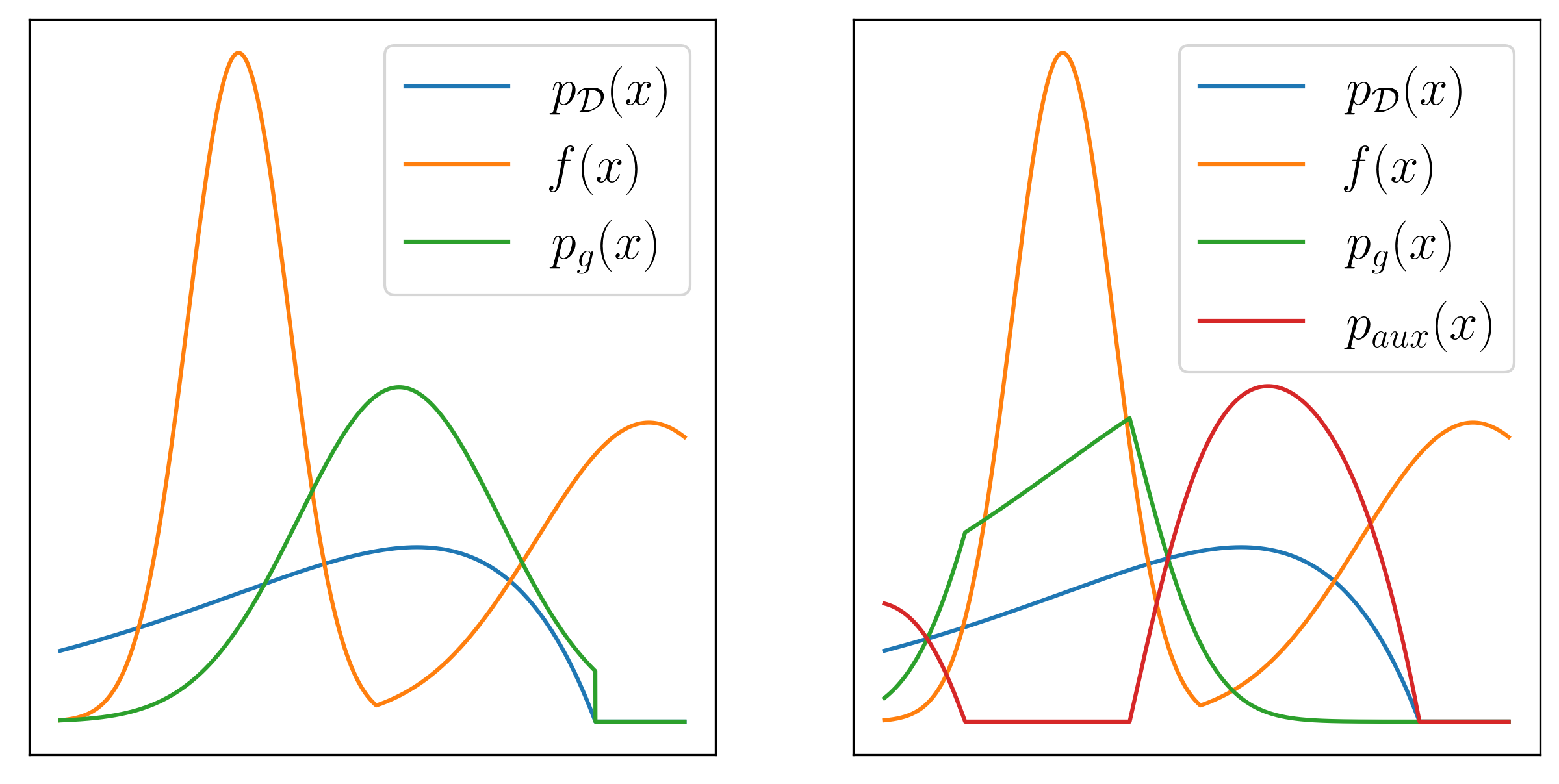
Figure 1: Visualizations to illustrate the benefit of dual generators over single generator when maximizing a secondary objective $f(x)$ in the GAN framework. In both figures, $p_{\mathcal{D}}(x)$ is the data distribution. The x-axis is a one-dimensional sample space. Left: In this figure, since there is only a single generator, the generator $G$ is trained to jointly maximize the objective $f(x)$ and matches the data distribution $p_{\mathcal{D}}(x)$. The distribution $p_{G}$ induced by the generator is thus not very good at either maximizing the objective $f(x)$ or matching the data distribution. Right: In this figure, we have two generators, inducing two distributions $p_{G}$ and $p_{aux}$. By introducing the auxiliary generator $G_{aux}$ into the GAN framework, the primary generator can better maximize the objective $f(x)$ while staying within the support of the data distribution $p_{\mathcal{D}}$. The mixed distribution also perfectly matches the data distribution, i.e. $\dfrac{p_{g}(x)+p_{aux}(x)}{2}=p_{\mathcal{D}}(x)$. Note that in these two figures, the primary generator aims to maximize $f(x)$ (instead of minimize) to allow for more intuitive interpretation. In Appendix B, we provide a numerical example to further illustrate the benefit of the dual generator technique on a 1D example.

In this section, we will develop an approach for performing a joint optimization of adversarial and secondary objectives of the generator in a GAN framework, which we will then apply to offline RL. This is a necessary component for performing the joint optimization in Eq. 2 without introducing a conflict of these objectives. All proofs for theorems presented in this section are in Appendix A.

Let’s consider a general objective that requires training a generator $G$ to fool the discriminator $D$ while also optimizing the expected value of some other function $f$:

$$\min_{G}\max_{D}\quad \mathbb{E}_{x\sim p_{\mathcal{D}}}[\log(D(x))]$$

$$+\hskip 3.00003pt \mathbb{E}_{z\sim p(z)}[\log(1-D(G(z)))]$$

$$+\hskip 3.00003pt \mathbb{E}_{z\sim p(z)}[f(G(z))]$$ (4)

where the first two terms are the same as the objective of the GAN formulation. We have also added an additional term $\mathbb{E}_{z\sim p(z)}[f(G(z))]$, where $f$ is a mapping from the generator output to a scalar value. The third term represents a secondary objective that the generator should optimize.

Theorem 4.1

The optimal generator of Eq. 4 induces a distribution $p^{*}_{g}(x)=p_{\mathcal{D}}(x)\dfrac{e^{-f(x)-\nu}}{2-e^{-f(x)-\nu}}$, where $\nu>0$ is the Lagrange multiplier that ensures that $p^{*}_{g}(x)$ is normalized to 1.

We can see that by adding a secondary objective function for the generator, in general, the optimal generator does not attempt to match the data distribution $p_{\mathcal{D}}(x)$ anymore, but instead tries to match the data distribution weighted by $\dfrac{e^{-f(x)-\nu}}{2-e^{-f(x)-\nu}}$. We expect that in such case, the discriminator clearly has an advantage in the two player zero-sum game and will be able to distinguish between real samples and sample generated by the generator.

To allow the generator to specialize in optimizing the secondary objective function, we propose to introduce a second auxiliary generator that matches the portion of the data distribution that is not well captured by the primary generator. Let $p_{mix}=\dfrac{p_{g}+p_{aux}}{2}$, consider the min-max problem:

$$\min_{G,G_{aux}}\max_{D}\mathbb{E}_{x\sim p_{\mathcal{D}}}[\log(D(x))]+\mathbb{E}_{x\sim p_{mix}}[\log(1-D(x))]+\mathbb{E}_{x\sim p_{g}}[f(x)],$$ (5)

where we mix samples from the primary generator $G$ and the auxiliary generator $G_{aux}$ to generate samples that can fool the discriminator. The mixing is indicated by the distribution $p_{mix}$ in the second term of Eq. 5. The first and third term of Eq. 5 are the same as the objective in Eq. 4.

We next theoretically demonstrate the benefit of adding the auxiliary generator to the GAN formulation with the following Theorem.

Theorem 4.2 (Informal)

The primary generator $p_{G}$ performs in-support optimization of $f(x)$.

We first note that the optimal solution of the mixed distribution from Eq. 5 is the real data distribution:

$$\dfrac{p^{*}_{aux}(x)+p^{*}_{g}(x)}{2}=p_{\mathcal{D}}(x)$$ (6)

Accordingly, the optimal auxiliary generator distribution can be expressed as

$$p^{*}_{aux}(x)=2p_{\mathcal{D}}(x)-p^{*}_{g}(x)$$ (7)

Let $x_{0}$ to be the element inside the support of the data distribution $p_{\mathcal{D}}$ that minimizes $f$. That is:

$$x_{0}=\underset{x\in\text{Supp}(p_{\mathcal{D}})}{\arg\min}f(x)$$

When optimizing the secondary objective $f(x)$, the primary generator will maximize the probability mass of in-support samples that maximize $f(x)$. However, Eq. 7 introduces a constraint that enforces $2p_{\mathcal{D}}(x)-p^{*}_{g}(x)\geq 0$ for $p^{*}_{aux}(x)\geq 0$ to remain a valid distribution. This leads us to conclude that the optimal primary generator $p^{*}_{g}$ assigns the following probability to $x_{0}$:

$$p^{*}_{g}(x_{0}) =\begin{cases}2p_{\mathcal{D}}(x_{0})\quad\text{if}\quad 2p_{\mathcal{D}}(x_{0})<1\\ 1\quad\quad\quad\quad\text{otherwise}\end{cases}$$ (8)

Interestingly, if the global optimum $x_{0}$ is not taking the full probability mass, the rest of the probability mass is redistributed to the next best in-support optimum, which we can define recursively:

$$\text{For}\,\,x_{i}\in\underset{x\in\text{Supp}(p_{\mathcal{D}})\setminus\{x_{j}\}_{j=0}^{i-1}}{\arg\min}f(x),\,\,p^{*}_{g}(x_{i}) =\begin{cases}2p_{\mathcal{D}}(x_{i})\quad\quad\quad\quad\quad\text{if}\quad\sum_{j=0}^{i}p^{*}_{g}(x_{j})<1\\ 1-\sum_{j=0}^{i-1}p^{*}_{g}(x_{j})\quad\,\,\text{if}\quad\sum_{j=0}^{i}p^{*}_{g}(x_{j})>1\\ 0\quad\quad\quad\quad\quad\quad\quad\quad\text{if}\quad\sum_{j=0}^{i-1}p^{*}_{g}(x_{j})=1\end{cases}$$ (9)

We provide more explanation for the solution in Eq. 9. In the first case, $p^{*}_{g}(x_{i})=2p_{\mathcal{D}}(x_{i})$ if $\sum_{j=0}^{i}p^{*}_{g}(x_{j})<1$. That is, if the optimal solution for the primary generator $p^{*}_{g}$ can assign the probability $2p_{\mathcal{D}}(x_{i})$ to the $i^{th}$ in support minima of $f(x)$ without the total sum of probability assigned $\sum_{j=0}^{i}p^{*}_{g}(x_{j})$ going over $1$, then the primary generator $p^{*}_{g}$ will assign the probability $2p_{\mathcal{D}}(x_{i})$ to $x_{i}$.

In the second case, $p^{*}_{g}(x_{i})=1-\sum_{j=0}^{i-1}p^{*}_{g}(x_{j})$ if $\sum_{j=0}^{i}p^{*}_{g}(x_{j})>1$. That is, if by assigning the probability $2p_{\mathcal{D}}(x_{i})$ to the $i^{th}$ in support minima of $f(x)$, the total sum of probability assigned $\sum_{j=0}^{i}p^{*}_{g}(x_{j})$ goes over $1$, then the primary generator $p^{*}_{g}$ will assign the remaining probability $1-\sum_{j=0}^{i-1}p^{*}_{g}(x_{j})$ to $x_{i}$. In the third case, the generator assigns probability $0$ to $x_{i}$ because all the probability has already been assigned.

To summarize the benefit of dual generator, we note that by introducing an auxiliary generator and mixing it with the primary generator, not only does the optimal solution for the mixed distribution match the real data distribution, but also the primary generator can better optimize the secondary objective $f$ on the part of the domain of $f$ that is within the support of the data distribution $p_{\mathcal{D}}$. To better illustrate the benefit, we provide a visual explanation of the benefit in Figure 1.

4.2 Update rules for offline reinforcement learning

We will now incorporate the dual-generator method to train policies for offline RL, based on optimizing the joint objective from Eq. 5. The updates for the actor and the critic are generally similar to Eq. 3. However, simply combining Eq. 5 and Eq. 3 can still allow the policy to exploit errors in the value function during the policy improvement step. We therefore augment the policy improvement step with an adaptive weight on the Q-value.

More concretely, as the policy improvement step samples actions from the current policy iterate $\pi^{k}$ to optimize the policy objective, ’, as we observe in our experiments. To alleviate this issue, we use the probability assigned to the sampled actions by the discriminator to weight the value function estimates in the policy objective, leading to the following updates:

$$Q^{k+1}\leftarrow \operatorname*{arg\,min}_{Q}\mathbb{E}_{s,a,s^{\prime}\sim\mathcal{D}}\left[\left((R(s,a)+\gamma\mathbb{E}_{a^{\prime}\sim{\pi}^{k}(a^{\prime}|s^{\prime})}[Q^{k}(s^{\prime},a^{\prime})])-Q_{target}(s,a)\right)^{2}\right]$$ (10)

$$\pi^{k+1}\leftarrow \operatorname*{arg\,max}_{\pi}\mathbb{E}_{s,a_{\mathcal{D}}\sim\mathcal{D},a\sim\pi^{k}(a|s)}\left[\dfrac{D^{k}(s,a)}{D^{k}(s,a_{\mathcal{D}}(s))}Q^{k+1}(s,a)+\log D^{k}(s,a)\right],$$ (11)

where $a_{\mathcal{D}}(s)$ is the action from the offline dataset. The term $D^{k}(s,a)$ down-weights the contribution of the gradient of the value function to the policy update if the discriminator deems the sampled action too unlikely. We further calibrate the probability $D^{k}(s,a)$ by dividing it with the probability $D^{k}(s,a_{\mathcal{D}}(s))$ that the discriminator assigns to the dataset action $a_{\mathcal{D}}(s)$. It should be noted that during optimization the gradients are not propagated into these weights.

Next, we define the update rules for the auxiliary generator and the discriminator. We mix the samples from the $k^{th}$ iterate of the policy $\pi^{k}$ and the distribution $p_{aux}$ induced by the $k^{th}$ iterate of the auxiliary generator $G^{k}_{aux}$, that is, let $p_{mix}=\dfrac{\pi^{k}+p_{aux}}{2}$. At every iteration $k$, we update the $k^{th}$ iterate of the auxiliary generator $G^{k}_{aux}$ and discriminator $D^{k}$ using the objectives:

$$G^{k+1}_{aux}\leftarrow \operatorname*{arg\,min}_{G_{aux}}\mathbb{E}_{x\sim p_{mix}}[\log(1-D^{k}(s,a))]$$ (12)

$$D^{k+1}\leftarrow \operatorname*{arg\,max}_{D}\mathbb{E}_{x\sim p_{\mathcal{D}}}[\log(D^{k}(s,a))]+\mathbb{E}_{x\sim p_{mix}}[\log(1-D^{k}(s,a))]$$ (13)

4.3 Algorithm summary

Algorithm 1 provides a step-by-step description of our algorithm. At every training step, we sample a batch of transitions from the offline dataset and proceed to update the parameters of the value function, the policy, the auxiliary generator and the discriminator in that order.

1:  Initialize Q-function $Q_{\theta}$, policy $\pi_{\phi}$, auxiliary generator $G_{aux,\psi}$, discriminator $D_{\omega}$

2:  for training step $k$ in {1,…,N} do

3:     $(s,a,r,s^{\prime})\leftarrow\mathcal{D}$: Sample a batch of transitions from the dataset

4:     $\theta^{k+1}\leftarrow$ Update Q-function $Q_{\theta}$ using the Bellman update in Eq. 10

5:     $\phi^{k+1}\leftarrow$ Update policy $\pi_{\phi}$ using the augmented objective in Eq. 11

6:     $\psi^{k+1}\leftarrow$ Update auxiliary generator $G_{aux,\psi}$ using the objective in Eq. 12

7:     $\omega^{k+1}\leftarrow$ Update discriminator $D_{\omega}$ using mixed samples from $\pi_{\phi}$ and $G_{aux,\psi}$ as in Eq. 13

Algorithm 1 DASCO algorithm summary

5 Experiments

Our experiments aim at answering the following questions:

1. When learning from offline datasets that require combining actions from sub-optimal trajectories, does DASCO outperform existing methods that are based on distribution constraints?

2. On standard benchmarks such as D4RL Fu et al. (2020), how does DASCO compare against recent methods?

3. Are both the dual generator and the probability ratio weight important for the performance of DASCO?

5.1 Comparisons on standard benchmarks and new datasets

For our first set of experiments, we introduce four new datasets to simulate the challenges one might encounter when using offline RL algorithms on real world data. These datasets introduce additional learning challenges and require the algorithm to combine actions in different trajectories to obtain good performance. We use the existing AntMaze environments from the D4RL suite Fu et al. (2020): antmaze-medium and antmaze-large. In these two environments, the algorithm controls an 8-DoF “Ant" quadruped robot to navigate a 2D maze to reach desired goal locations. The D4RL benchmark generates the offline datasets for these two environments using two policies: 1. a low-level goal reaching policy that outputs torque commands to move the Ant to a nearby goal location and 2. a high-level waypoint generator to provide sub-goals that guide the low-level goal-reaching policy to the desired location. We use the same two policies to generate two new classes of datasets.

For the noisy dataset, we add Gaussian noise to the action computed by the low-level goal-reaching policy. The noise variance depends on the 2D location of the Ant in the maze – larger in some 2D regions than others. We intend this dataset to be representative of situations where the data generation policies are more deterministic in some states than others Kumar et al. (2022) – a robot picking up an object has many good options to approach the object, but when the robot grasps the object, its behavior should be more deterministic to ensure successful grasp without damaging or dropping the object Murray et al. (1994).

For a biased dataset, in addition to adding Gaussian noise to the actions as it is done in the noisy dataset, we also add bias to the actions computed by the low-level policy. The values of the bias also depend on the current 2D location of the Ant in the maze. This setting is meant to simulate learning from relabelled data, where the dataset was generated when the data generation policies were performing a different task than the tasks we are using the dataset to learn to perform. Relabelling offline data is a popular method for improving the performance of offline RL algorithms Vuong et al. (2019); Snell et al. (2022), especially when we have much more data for some tasks than others Kalashnikov et al. (2021). In the AntMaze environment, offline RL algorithms must combine data from sub-optimal trajectories to learn behaviors with high returns. In addition, noisy and biased datasets present a more challenging learning scenarios due to the added noise and systematic bias which vary non-uniformly based on the 2D location of the Ant.

Table 1 illustrates the performance comparison of our method and representative methods that enforce distribution constraints, either through optimizing a conservative lower bound of the value estimates (CQL) or only optimizing the policy on actions in the dataset using Advantage Weighted Regression Peng et al. (2019) (IQL). Our method outperforms both CQL and IQL. In these tasks, to ensure a fair comparison between different methods, we perform oracle offline policy selection to obtain the performance estimates for CQL, IQL, and our method. We describe how we tune hyper-parameters for the baselines in Appendix E. We also include results of recent methods, such as EDAC An et al. (2021) and BEAR Kumar et al. (2019a). We also compare the performance on standard AntMaze tasks when learning from the datasets in the D4RL benchmark without modifications in Table 2. In these tasks, our method outperforms IQL by a large margin on two diverse datasets.

Table 1: Performance comparison to baselines when learning from the noisy and biased AntMaze datasets. Our method outperforms the baselines significantly. The value in parenthesis indicates the standard deviation of mean episode return, computed over 3 different runs.

Dataset	BEAR	EDAC	CQL	IQL	DASCO (Ours)
antmaze-large-bias	-	-	61.7 (3.5)	41.0 (7.9)	63.9 (6.0)
antmaze-large-noisy	-	-	50.3 (2.3)	39.0 (6.4)	54.3 (2.0)
antmaze-medium-bias	0.0 (0.0)	0.0 (0.0)	66.7 (2.9)	48.0 (5.9)	90.2 (2.4)
antmaze-medium-noisy	0.0 (0.0)	0.0 (0.0)	55.7 (4.7)	44.3 (1.7)	86.3 (4.5)
noisy and biased antmaze-v2 total	-	-	234.4	172.3	294.7

Table 2: Performance comparison to distribution-constrained baselines on AntMaze tasks in D4RL. Our algorithm outperforms the baselines when learning from the diverse and play datasets.

Dataset	CQL	IQL	DASCO (Ours)
antmaze-umaze	97.0 (0.8)	90.3 (1.9)	99.2 (0.0)
antmaze-umaze-diverse	58.7 (12.2)	70.3 (4.6)	89.0 (1.7)
antmaze-medium-play	77.0 (1.6)	82.7 (0.5)	92.3 (1.5)
antmaze-medium-diverse	80.0 (0.0)	82.3 (1.9)	87.1 (0.4)
antmaze-large-play	53.3 (4.6)	55.7 (3.1)	64.4 (1.7)
antmaze-large-diverse	48.0 (2.9)	50.0 (3.6)	74.1 (2.8)
antmaze total	414.0	431.3	506.1

Table 3: Performance comparison with recent offline RL algorithms on the Gym locomotion tasks

Dataset	BC	10%BC	DT Chen et al. (2021)	AWAC Nair et al. (2020)	Onestep RL Brandfonbrener et al. (2021b)	TD3+BC Fujimoto and Gu (2021b)	COMBO Yu et al. (2021)	CQL	IQL	DASCO (Ours)
halfcheetah-medium-replay	36.6	40.6	36.6	40.5	38.1	44.6	55.1	45.5	44.2	44.7
hopper-medium-replay	18.1	75.9	82.7	37.2	97.5	60.9	89.5	95.0	94.7	101.7
walker2d-medium-replay	26.0	62.5	66.6	27.0	49.5	81.8	56.0	77.2	73.9	74.5
halfcheetah-medium-expert	55.2	92.9	86.8	42.8	93.4	90.7	90.0	91.6	86.7	93.8
hopper-medium-expert	52.5	110.9	107.6	55.8	103.3	98.0	111.1	105.4	91.5	110.9
walker2d-medium-expert	107.5	109.0	108.1	74.5	113.0	110.1	103.3	108.8	109.6	109.3
locomotion total	295.9	491.8	488.4	277.8	494.8	486.1	505	523.5	500.6	534.9

By comparing the results in Table 1 (learning from noisy and biased datasets) and Table 2 (learning from existing offline datasets in D4RL), we also note that our proposed algorithm outperforms distribution-constraint offline RL algorithms (CQL, IQL) more consistently when tested on the noisy and biased datasets. For the results in these two tables, the definition of the antmaze-medium and antmaze-large environments are the same. The only axis of variation in the learning setup is the noise and systematic bias added to the actions of the dataset generation policies. We therefore conclude that our algorithm is more robust to the noise and systematic bias added to the actions than distribution-constrained offline RL algorithms.

Next, we evaluate our approach on Gym locomotion tasks from the standard D4RL suite. The performance results on these tasks are illustrated in Table 3. Our method is competitive with BC, one-step offline RL methods Brandfonbrener et al. (2021a), and multi-step distribution-constraint RL methods Kostrikov et al. (2021b); Kumar et al. (2020). This is not surprising because in these tasks, the offline dataset contains a large number of trajectories with high returns. In Table 3, 10%BC refers to performing BC using the top $10\%$ trajectories with the highest episode return.

5.2 Ablations

We conduct three different sets of experiments to gain more insights into our algorithm. The first experiment measures the importance of having an auxiliary generator. We recall that there are two benefits to having the auxiliary generator. Firstly, without the auxiliary generator, the generator does not in general match the data distribution (4.1). As such, the discriminator has an unfair advantage in learning how to distinguish between real and generated examples. Secondly, the auxiliary generator plays the role of a support player and learns to output actions that are assigned non-zero probability by the data distribution, but have low Q values. The support player allows the policy to concentrate on in-support maximization of the Q-function (4.2). Table 4 demonstrates that having an auxiliary generator clearly leads to a performance improvement across different task families, from Gym locomotion tasks to AntMaze navigation tasks.

The second experiment compares the performance of the policy and the auxiliary generator on a subset of the Gym locomotion and AntMaze tasks (Table 5). The difference in the performance of the policy and auxiliary generator illustrates their specialization of responsibility: the policy learns to output actions that lead to good performance, while the auxiliary generator learns to model the “remainder" of the data distribution. If this “remainder" also contains good action, then the auxiliary generator will have non-trivial performance. Otherwise, the auxiliary generator will have poor performance.

In the Gym locomotion tasks, the auxiliary generator has non-trivial performance, but it is still worse than the policy. This demonstrates that: 1. By optimizing the policy to maximize the long-term return and the discriminator function, the policy can outperform the auxiliary generator, which only maximizes the discriminator function, 2. The dataset contains a large fraction of medium performance level actions contained in continuous trajectories, which the auxiliary generator has learnt to output. In contrast, in the bias and noisy AntMaze tasks, the auxiliary generator fails to obtain non-zero performance while the policy has strong performance. This reflects the necessity of carefully picking a subset of the in-support actions to obtain good performance.

Table 4: Ablation for training without and with auxiliary generator. The dual generator technique, which trains the auxiliary generator in addition to the policy, is crucial to obtain good performance.

Dataset	Without	With
halfcheetah-medium-expert	79.8 (3.4)	93.8 (0.1)
hopper-medium-expert	95.1 (1.6)	110.9 (0.8)
antmaze-large-bias	55.0 (2.3)	63.9 (6.0)
antmaze-large-noisy	45.1 (1.8)	54.3 (2.0)

Table 5: Policy vs Auxiliary Generator. The auxiliary generator has reasonable performance on the easier locomotion tasks and is significantly worse than the policy on the harder AntMaze tasks.

Dataset	Auxiliary Generator	Policy
halfcheetah-medium-expert	48.5 (2.1)	93.8 (0.1)
hopper-medium-expert	70.4 (0.9)	110.9 (0.8)
antmaze-large-bias	0.0 (0.0)	63.9 (6.0)
antmaze-large-noisy	0.0 (0.0)	54.3 (2.0)

The third set of experiments illustrates the importance of weighing the value function in the policy objective by the probability computed by the discriminator, as described in Eq. 11. Doing so provides a second layer of protection against exploitation of errors in the value function by the policy. Table 6 illustrates that this is very important for the AntMaze tasks, which require combining optimal and sub-optimal trajectories to obtain good performance. Perhaps this is because learning from such trajectories necessitates many rounds of offline policy evaluation and improvement steps, with each round creating an opportunity for the policy to exploit the errors in the value estimates. On the other hand, the dynamic weight is less important in the Gym locomotion tasks, presumably because a significant fraction of the corresponding offline datasets has high returns and therefore incorporating sub-optimal data is less criticial to obtain high performance.

Table 6: Ablation for dynamic weighting of value function estimates in the policy objective. When learning from datasets that require combining actions across trajectories, such as the AntMaze tasks, using the dynamic weighting is vital to obtaining good performance.

Dataset	Without	With
halfcheetah-medium-expert	91.1 (1.1)	93.8 (0.1)
hopper-medium-expert	106.7 (2.9)	110.9 (0.8)
antmaze-large-play	0.0 (0.0)	64.4 (1.7)
antmaze-large-diverse	0.0 (0.0)	74.1 (2.8)

6 Conclusions

In this paper, we introduced DASCO, a GAN-based offline RL method that addresses the challenges of training policies as generators with a discriminator to minimize deviation from the behavior policy by means of two modifications: an auxiliary generator to turn the GAN loss into a support constraint, and a value function weight in the policy objective. The auxiliary generator makes it possible for the policy to focus on maximizing the value function without needing to match the entirety of the data distribution, only that part of it that has high value, effectively turning the standard distributional constraint that would be enforced by a conventional GAN into a kind of support constraint. This technique may in fact be of interest in other settings where there is a need to maximize some objective in addition to fooling a discriminator, and applications of this approach outside of reinforcement learning are an exciting direction for future work. Further, since our method enables GAN-based strategies to attain good results on a range of offline RL benchmark tasks, it would also be interesting in future work to consider other types of GAN losses that induce different divergence measures. We also plan to explore robust methods for offline policy and hyper-parameter selection in the future.

Potential negative societal impact Because our focus is on developing a generic offline RL algorithm and not its application in any particular domain, our method inherits the potential negative societal impacts that any offline RL algorithm might have, such as data bias and lack of robustness to distributional shift. We also note that how to perform effective offline policy selection and evaluation in the general case remain challenging. Therefore, the offline learned RL policies might not be easily deployed to solve real world problems where online policy evaluation is expensive.

Checklist

The checklist follows the references. Please read the checklist guidelines carefully for information on how to answer these questions. For each question, change the default [TODO] to [Yes] , [No] , or [N/A] . You are strongly encouraged to include a justification to your answer, either by referencing the appropriate section of your paper or providing a brief inline description. For example:

• Did you include the license to the code and datasets? [Yes] See Section LABEL:gen_inst.

• Did you include the license to the code and datasets? [No] The code and the data are proprietary.

• Did you include the license to the code and datasets? [N/A]

1. For all authors…

   1. Do the main claims made in the abstract and introduction accurately reflect the paper’s contributions and scope? [Yes]

   2. Did you describe the limitations of your work? [Yes] Please see the experimental results in Section 5 and avenues for future work in the Conclusion

   3. Did you discuss any potential negative societal impacts of your work? [Yes] We discussed the potential negative impacts in the Conclusion of the paper

   4. Have you read the ethics review guidelines and ensured that your paper conforms to them? [Yes]

2. If you are including theoretical results…

   1. Did you state the full set of assumptions of all theoretical results? [Yes] We will include the proofs for all theorems in the Appendix

   2. Did you include complete proofs of all theoretical results? [Yes] We will include the proofs for all theorems in the Appendix

3. If you ran experiments…

   1. Did you include the code, data, and instructions needed to reproduce the main experimental results (either in the supplemental material or as a URL)? [Yes] We will include these results in the Appendix

   2. Did you specify all the training details (e.g., data splits, hyperparameters, how they were chosen)? [Yes] We will include this information in the Appendix

   3. Did you report error bars (e.g., with respect to the random seed after running experiments multiple times)? [Yes] We will include this information in the Appendix

   4. Did you include the total amount of compute and the type of resources used (e.g., type of GPUs, internal cluster, or cloud provider)? [Yes] Please see Appendix D

4. If you are using existing assets (e.g., code, data, models) or curating/releasing new assets…

   1. If your work uses existing assets, did you cite the creators? [N/A]

   2. Did you mention the license of the assets? [N/A]

   3. Did you include any new assets either in the supplemental material or as a URL? [N/A]

   4. Did you discuss whether and how consent was obtained from people whose data you’re using/curating? [N/A]

   5. Did you discuss whether the data you are using/curating contains personally identifiable information or offensive content? [N/A]

5. If you used crowdsourcing or conducted research with human subjects…

   1. Did you include the full text of instructions given to participants and screenshots, if applicable? [N/A]

   2. Did you describe any potential participant risks, with links to Institutional Review Board (IRB) approvals, if applicable? [N/A]

   3. Did you include the estimated hourly wage paid to participants and the total amount spent on participant compensation? [N/A]

Appendices

Appendix A Proofs for theorems in Section 4.1

A.1 Proof for Theorem 4.1

In the following proof, we use $p_{\text{data}}$ to refer to the real data distribution, instead of $p_{\mathcal{D}}$ as in Section 4.1, to avoid confusion with the discriminator distribution.

We recall Theorem 4.1:

See 4.1

The optimization problem in Eq. 4 is:

$$\min_{G}\max_{D}V(G,D)=\mathbb{E}_{x\sim p_{\text{data}}}[\log(D(x))]+\mathbb{E}_{z\sim p(z)}[\log(1-D(G(z)))]+\mathbb{E}_{z\sim p(z)}[f(G(z))]$$

The proof proceeds as follows: We first simplify the objective function into two terms. The first term is the Jensen–Shannon divergence between the data distribution and the distribution induced by the generator Goodfellow et al. [2014a]. The second term is the expected value of the secondary objective function $f$. We then show that the problem is convex, where strong duality holds. We then use the KKT conditions to find the functional form of the optimal solution, which gives us Theorem 4.1.

We only prove the statement for discrete sample space, and we let $n$ be the size of the sample space – the random variable $x$ can take on $n$ different values.

Proof. Since the third term in the objective function is not a function of the discriminator $D$, for $G$ fixed, the optimal discriminator of Eq. 4 is $D^{*}_{G}(x)=\dfrac{p_{\text{data}}(x)}{p_{\text{data}}(x)+p_{g}(x)}$ where $p_{g}$ is the distribution induced by the generator $G$. (similar to Prop 1 in Goodfellow et al. [2014a] ).

Similarly to how Goodfellow et al. [2014a] shows that the GAN objective in Eq. 1 minimizes the JS divergence between the data distribution and the distribution induced by the generator, we can now rewrite the objective in Eq. 4 as:

$$V(G,D^{*}_{G})$$ (14)

$$=\mathbb{E}_{x\sim p_{\text{data}}}[\log(D^{*}_{G}(x))]+\mathbb{E}_{z\sim p(z)}[\log(1-D^{*}_{G}(G(z)))]+\mathbb{E}_{z\sim p(z)}[f(G(z))]$$ (15)

$$=2JSD(p_{\text{data}}||p_{g})+\mathbb{E}_{x\sim p_{g}}[f(x)]-\log 4$$ (16)

For conciseness, let $g^{(i)}=p_{g}(x_{i})$ be the probability that $p_{g}$ assigns to $x_{i}$ and $g=[g^{(1)},\ldots,g^{(n)}]^{T}$ be a column vector containing the probabilities that $p_{g}$ assigns to each possible values of $x$, from $x_{1}$ to $x_{n}$.

Similarly, let $f^{(i)}=f(x_{i})$ be the value that the secondary objective $f$ assigns to $x_{i}$. We also overload the notation to let $f=[f^{(1)},\ldots,f^{(n)}]^{T}$ be a column vector containing the values that the secondary objective $f$ assigns to each possible value of the random variable $x$, from $x_{1}$ to $x_{n}$.

Also let $p_{\text{data}}^{(i)}=p_{\text{data}}(x_{i})$ be the probability that the data distribution assigns to $x_{i}$.

We can then rewrite the problem in Eq. 4 in a standard form Boyd and Vandenberghe [2004] as:

$$\min_{g}\quad 2JSD(p_{\text{data}}||p_{g})+g^{T}f$$ (17)

s.t. $$-g^{(i)}\leq 0$$ (18)

$$\mathbf{1}^{T}g-1=0$$ (19)

where $\mathbf{1}$ is a column vector of $1$, which has the same number of entries as the vector $g$. The constraint 18 ensures that the probability that $p_{g}$ assigns to any $x$ is non-negative and the constraint 19 ensures the probabilities sum up to $1$.

The problem is convex because the objective function is a nonnegative weighted sum of two convex functions (JSD is convex because JSD is itself a nonnegative weighted sum of KL, which is a convex function).

Strong duality also holds because Slater’s condition holds. A strictly feasible point for Slater’s condition to hold is the uniform distribution, i.e. $g^{(i)}=\dfrac{1}{n},\forall i$.

The Lagrangian is:

$$L=2JSD(p_{\text{data}}||p_{g})+g^{T}f-\sum_{i}\lambda^{(i)}g^{(i)}+\nu(\mathbf{1}^{T}g-1)$$ (20)

where $\lambda^{(i)}$ and $\nu$ are the Lagrangian multipliers.

For any $i\in[1,n]$, the partial derivative of the Lagrangian with respect to $g^{(i)}$ is:

$$\pdv{L}{g^{(i)}} =log\left(\dfrac{2g^{(i)}}{p_{\text{data}}^{(i)}+g^{(i)}}\right)+f^{(i)}-\lambda^{(i)}+\nu$$ (21)

Let $g_{*}$ and $(\lambda_{*},\nu_{*})$ be the primal and dual optimal solutions of the optimization problem. As the strong duality holds, the variables $g_{*}$ and $(\lambda_{*},\nu_{*})$ must satisfy the KKT conditions. For any $i\in[1,n]$, the following holds:

$$-g_{*}^{(i)} \leq 0$$ (22)

$$\mathbf{1}^{T}g_{*}-1 =0$$ (23)

$$\lambda_{*}^{(i)} \geq 0$$ (24)

$$\lambda_{*}^{(i)}g_{*}^{(i)} =0$$ (25)

$$\pdv{L}{g^{(i)}}=log\left(\dfrac{2g_{*}^{(i)}}{p_{\text{data}}^{(i)}+g_{*}^{(i)}}\right)+f^{(i)}-\lambda_{*}^{(i)}+\nu_{*} =0$$ (26)

From Equation 26, we have $\lambda_{*}^{(i)}=log\left(\dfrac{2g_{*}^{(i)}}{p_{\text{data}}^{(i)}+g_{*}^{(i)}}\right)+f^{(i)}+\nu_{*}$, and substitute into Equation 25:

$$\left[log\left(\dfrac{2g_{*}^{(i)}}{p_{\text{data}}^{(i)}+g_{*}^{(i)}}\right)+f^{(i)}+\nu_{*}\right]g^{*}_{i} =0$$ (27)

We consider what happens when $g^{*}_{i}>0$, due to complementary slackness, we have:

$$\log\left(\dfrac{2g_{*}^{(i)}}{p_{\text{data}}^{(i)}+g_{*}^{(i)}}\right)+f^{(i)}+\nu_{*} =0$$ (28)

$$\Longrightarrow g_{*}^{(i)} =\dfrac{p_{\text{data}}^{(i)}e^{-f^{(i)}-\nu_{*}}}{(2-e^{-f^{(i)}-\nu_{*}})}$$ (29)

$$p^{*}_{g}(x_{i}) =p_{\text{data}}(x_{i})\dfrac{e^{-f(x_{i})-\nu_{*}}}{2-e^{-f(x_{i})-\nu_{*}}}$$ (30)

We can then pick an appropriate value for the Lagrange multiplier $\nu$ such that the probabilities $p^{*}_{g}(x_{i})$ normalize to 1. QED.

A.2 Proof for Theorem 4.2

In the following proof, we use $p_{\text{data}}$ to refer to the real data distribution, instead of $p_{\mathcal{D}}$ as in Section 4.1, to avoid confusion with the discriminator distribution.

Recall that we define $p_{mix}$ as $p_{mix}=\dfrac{p_{g}+p_{aux}}{2}$. Theorem 4.2 is stated in reference to the optimization problem in Eq. 5, which we restate here:

$$\min_{G,G_{aux}}\max_{D}\quad V(G,G_{aux},D)=\mathbb{E}_{x\sim p_{\text{data}}}[\log(D(x))]+\mathbb{E}_{x\sim p_{mix}}[\log(1-D(x))]+\mathbb{E}_{x\sim p_{g}}[f(x)]$$ (31)

where the first two terms in the objective function are the GAN objective and the last term is the secondary objective function.

Similar to the proof for Theorem 4.1, we can rewrite the objective function in Eq. 31 as Goodfellow et al. [2014a]:

$$V(G,G_{aux},D^{*})$$ (32)

$$=2JSD(p_{\text{data}}||\dfrac{p_{g}+p_{aux}}{2})+\mathbb{E}_{x\sim p_{g}}[f(x)]-\log 4$$ (33)

We are only interested in optimizing for the secondary objective function $f$ in the space of optimal GAN solutions. We therefore enforce that $p_{mix}=\dfrac{p_{g}+p_{aux}}{2}=p_{\text{data}}$, which makes the JSD term vanish in Eq. 33 and allows us to solve the following optimization problem.

$$\min_{G}\quad \mathbb{E}_{x\sim p_{g}}[f(x)]$$ (34)

s.t. $$p_{g}\leq 2p_{\text{data}}$$ (35)

$$p_{aux}=2p_{\text{data}}-p_{g}$$ (36)

We claim that the solution to the optimization problem above is as follows. We define $x_{0}$ to be the element inside the support of the data distribution $p_{\text{data}}$ that minimizes $f$, i.e. $x_{0}=\underset{x\in\text{Supp}(p_{\text{data}})}{\arg\min}f(x)$. The optimal primary generator $p^{*}_{g}$ assigns the following probability to $x_{0}$:

$$p^{*}_{g}(x_{0}) =\begin{cases}2p_{\text{data}}(x_{0})\quad\text{if}\quad 2p_{\text{data}}(x_{0})<1\\ 1\quad\quad\quad\quad\text{otherwise}\end{cases}$$ (37)

If the global maximum $x_{0}$ is not taking the full probability mass, the rest of the probability mass is redistributed to the next best in-support maxima, which we can define recursively:

$$\text{For}\,\,x_{i}\in\underset{x\in\text{Supp}(p_{\text{data}})\setminus\{x_{j}\}_{j=0}^{i-1}}{\arg\min}f(x),\,\,p^{*}_{g}(x_{i}) =\begin{cases}2p_{\text{data}}(x_{i})\quad\quad\quad\quad\,\,\,\text{if}\quad\sum_{j=0}^{i}p^{*}_{g}(x_{j})<1\\ 1-\sum_{j=0}^{i-1}p^{*}_{g}(x_{j})\quad\,\,\text{if}\quad\sum_{j=0}^{i}p^{*}_{g}(x_{j})>1\\ 0\quad\quad\quad\quad\quad\quad\quad\quad\text{if}\quad\sum_{j=0}^{i-1}p^{*}_{g}(x_{j})=1\end{cases}$$ (38)

Proof.

We show the proof by contradiction. That is, assume that there exists another distribution $p^{a}_{g}$ with the following properties:

• There exists $x$ where $p^{a}_{g}(x)\neq p_{g}^{*}(x)$

• $p^{a}_{g}$ satisfies the constraint (35)-(36)

• The value of the objective function achieved by $p^{a}_{g}$ is better than the value achieved by $p_{g}^{*}$. That is, $\mathbb{E}_{x\sim p^{a}_{g}}[f(x)]<\mathbb{E}_{x\sim p^{*}_{g}}[f(x)]$.

We will show that the existence of such a distribution $p^{a}_{g}$ will lead to contradiction,

We separate the analyses into three different cases, depending on the property of $p_{g}^{*}$:

• Case 1: $p_{g}^{*}$ assigns all probability mass to $x_{0}$

• Case 2: If $p_{g}^{*}$ assigns non-zero probability to $x$, then $p_{g}^{*}=2p_{\text{data}}(x)$

• Case 3: There exists an $x$ where $2p_{\text{data}}(x)>p_{g}^{*}(x)>0$

We will walk through the three cases independently and show the contradiction in each case.

Case 1: $p^{*}_{g}$ assigns the full probability mass to $x_{0}$, that is $p^{*}_{g}(x_{0})=1$, and assigns zero probability to every $x$ not equal to $x_{0}$. Without loss of generality, we consider $p_{g}$ that assigns non-zero probability to a $x_{k}\neq x_{0}$, assigns the remaining probability mass to $x_{0}$, and assigns zero probability to all $x$ that is not equal to either $x_{0}$ or $x_{k}$. That is, assume there exists $p^{a}_{g}$ such that:

$$0>p^{a}_{g}(x_{0}) >1$$ (39)

$$p^{a}_{g}(x_{k}) =1-p^{a}_{g}(x_{0})>0\text{ for some }x_{k}\in\text{Supp}(p_{\text{data}})$$ (40)

$$\mathbb{E}_{x\sim p^{*}_{g}}[f(x)]-\mathbb{E}_{x\sim p^{a}_{g}}[f(x)] >0$$ (41)

where $x_{k}\in\text{Supp}(p_{\text{data}})$ follows from constraint 35 ($p_{g}\leq 2p_{\text{data}}$, and thus $p^{a}_{g}$ can only assign non-zero probability to $x$ within the support of $p_{\text{data}}$). We can then show that:

$$\mathbb{E}_{x\sim p^{*}_{g}} [f(x)]-\mathbb{E}_{x\sim p^{a}_{g}}[f(x)]$$ (42)

$$= f(x_{0})-p^{a}_{g}(x_{0})f(x_{0})-p^{a}_{g}(x_{k})f(x_{k})$$ (43)

$$= (1-p^{a}_{g}(x_{0}))f(x_{0})-p^{a}_{g}(x_{k})f(x_{k})$$ (44)

$$= p^{a}_{g}(x_{k})f(x_{0})-p^{a}_{g}(x_{k})f(x_{k})$$ (45)

$$= p^{a}_{g}(x_{k})[f(x_{0})-f(x_{k})]\leq 0\text{ (contradiction with Eq.}\ref{eq:case_1_contra})$$ (46)

where the last inequity follows from these two facts:

$$x_{0} =\underset{x\in\text{Supp}(p_{\text{data}})}{\arg\min}f(x)$$ (47)

$$x_{k} \in\text{Supp}(p_{\text{data}})$$ (48)

Case 2:

$$p^{*}_{g}(x) =\begin{cases}2p_{\text{data}}(x)\quad\text{if}\quad p^{*}_{g}(x)>0\\ 0\quad\quad\quad\quad\text{otherwise}\end{cases}$$ (49)

Let $\{x_{0},\ldots,x_{i}\}$ be the set of x where $p^{*}_{g}(x)>0$, then we also require that $\sum_{j=0}^{i}p^{*}_{g}(x)=1$.

Without loss of generality, we assume a distribution $p^{a}_{g}$ exists with the following properties. There exists $x_{m},x_{n}$ such that:

$$p^{*}_{g}(x_{m})=2p_{\text{data}}(x_{m})>0\quad \text{ and }\quad p^{a}_{g}(x_{m})<2p_{\text{data}}(x_{m})$$ (50)

$$p^{*}_{g}(x_{n})=0\quad \text{ and }\quad p^{a}_{g}(x_{n})=2p_{\text{data}}(x_{m})-p^{a}_{g}(x_{m})>0$$ (51)

$$p^{*}_{g}(x) =p^{a}_{g}(x)\text{ otherwise (that is, for all }x\notin\{x_{m},x_{n}\})$$ (52)

$$\mathbb{E}_{x\sim p^{*}_{g}}[f(x)]-\mathbb{E}_{x\sim p^{a}_{g}}[f(x)] >0$$ (53)

We note that $f(x_{m})\leq f(x_{n})$ since $p^{*}_{g}$ assigns non-zero probability to $x_{m}$ and assigns zero probability to $x_{n}$.

We can show that:

$$\mathbb{E}_{x\sim p^{*}_{g}} [f(x)]-\mathbb{E}_{x\sim p^{a}_{g}}[f(x)]$$ (54)

$$= p^{*}_{g}(x_{m})f(x_{m})-p^{a}_{g}(x_{m})f(x_{m})-p^{a}_{g}(x_{n})f(x_{n})$$ (55)

$$= p^{*}_{g}(x_{m})f(x_{m})-p^{a}_{g}(x_{m})f(x_{m})-p^{a}_{g}(x_{n})f(x_{n})$$ (56)

$$= p^{*}_{g}(x_{m})f(x_{m})-p^{a}_{g}(x_{m})f(x_{m})-(2p_{\text{data}}(x_{m})-p^{a}_{g}(x_{m}))f(x_{n})$$ (57)

$$= p^{*}_{g}(x_{m})f(x_{m})-p^{a}_{g}(x_{m})f(x_{m})-2p_{\text{data}}(x_{m})f(x_{n})+p^{a}_{g}(x_{m})f(x_{n})$$ (58)

$$= p^{*}_{g}(x_{m})f(x_{m})-p^{a}_{g}(x_{m})f(x_{m})-p^{*}_{g}(x_{m})f(x_{n})+p^{a}_{g}(x_{m})f(x_{n})$$ (59)

$$= p^{*}_{g}(x_{m})[f(x_{m})-f(x_{n})]-p^{a}_{g}(x_{m})[f(x_{m})-f(x_{n})]$$ (60)

$$= [f(x_{m})-f(x_{n})][p^{*}_{g}(x_{m})-p^{a}_{g}(x_{m})]\leq 0\text{ (contradiction with Eq.}\ref{eq:case_2_contra})$$ (61)

where the last inequality is true because $f(x_{m})\leq f(x_{n})$ as we noted above, and $p^{*}_{g}(x_{m})=2p_{\text{data}}(x_{m})>p^{a}_{g}(x_{m})$.

Case 3:

There exists $x_{i}$ such that $2p_{\text{data}}(x_{i})>p^{*}_{g}(x_{i})>0$. For all $x\neq x_{i}$:

$$p^{*}_{g}(x) =\begin{cases}2p_{\text{data}}(x)\quad\text{if}\quad p^{*}_{g}(x)>0\\ 0\quad\quad\quad\quad\text{otherwise}\end{cases}$$ (62)

Let $\{x_{0},\ldots,x_{i}\}$ be the set of x where $p^{*}_{g}(x)>0$, we also require $\sum_{j=0}^{i}p^{*}_{g}(x)=1$.

Without loss of generality, there are three cases we need to consider for the distribution $p^{a}_{g}$, each yielding a contradiction:

• $p^{a}_{g}(x_{i})=p^{*}_{g}(x_{i})$, but there exists $x$ such that $p^{a}_{g}(x)\neq p^{*}_{g}(x)$.

• $p^{a}_{g}(x_{i})>p^{*}_{g}(x_{i})$.

• $p^{a}_{g}(x_{i})<p^{*}_{g}(x_{i})$.

In each case, the proof by contradiction is similar to the proof in Case 2 above, where we pick a pair of $x_{m},x_{n}$ and shows that $p^{a}_{g}$ can not achieve a lower value of the objective function than $p^{*}_{g}$. We thus do not repeat the argument here. QED

Appendix B Benefits of dual generator technique on 1D discrete example

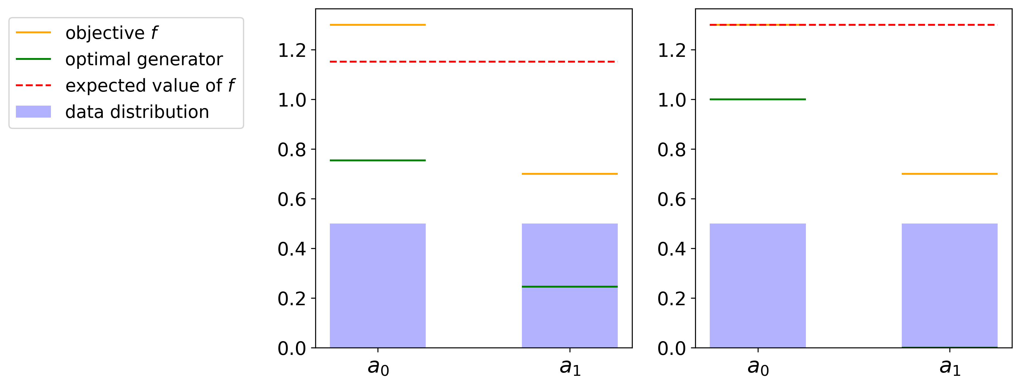
Figure 2: Left: We use a single generator. Right: We use dual generator technique. The optimal generator (green bar) refers to the optimal primary generator, and not the auxiliary generator. Thanks to the dual generator technique, the optimal primary generator in the right figure assigns probability $1.0$ to the global maxima $a_{0}$ of the secondary objective function $f$. The optimal primary generator in the right figure is therefore better at maximizing the function $f$ than the optimal generator in the left figure. Note that in this example, the generator aims to maximize the function $f$ (instead of minimize) for more intuitive interpretation.

In this section, we provide a simple one-dimensional numerical example with discrete action space to illustrate the benefit of the dual generator technique. In this example, the action space only consists two actions $a_{0},a_{1}$. The probability of action $a_{0}$ under the data distribution is $0.5$. The probability of action $a_{1}$ under the data distribution is $0.5$. We would like to maximize a secondary objective function $f$. The function $f$ assigns value $1.3$ to $a_{0}$ and value $0.7$ to $a_{1}$.

We will next show in a self-contained Jupyter notebook that when using only a single generator, the expected value of the secondary objective function $f$ under the optimal generator is $1.15$. We also show that when using the dual generator technique, the expected value of the secondary objective function $f$ under the optimal primary generator is $1.3$. Since $1.3$ is higher than $1.15$, we can see that using the dual generator technique allows us to better maximize the objective function $f$.

Fig 2 visually illustrates the benefits of the dual generator technique over using only a single generator in this example. We can also observe from Fig 2 (Left) that the optimal generator is clearly different from the data distribution when only using a single generator. As such, in the GAN framework, the discriminator has an advantage in learning how to distinguish between samples from the real data distribution and samples from the generator. In contrast, when using the dual generator technique, the optimal primary generator assigns probability $1$ to action $a_{0}$ and the optimal auxiliary generator assigns probability $1$ to action $a_{1}$ (not shown in Fig 2). Their mixed distribution therefore assigns probability $0.5$ to either actions, matching the data distribution.

The Jupyter notebook in the next page illustrates the computations necessary to obtain the optimal solution for the generator.

See pages - of maximize_version_without_code_to_draw_figures.pdf

Appendix C Description of the offline dataset generation procedure for the noisy and biased AntMaze datasets

In the experiments section, we introduce the bias and noisy datasets for the AntMaze tasks. In this section, we provide more details on how the datasets were generated in the form of Python syntax in Code Listing 1. We plan to open-source both the datasets and the code to generate the datasets upon acceptance.

Listing 1: Illustration of the dataset generation procedure for the bias and noisy datasets. Given an action computed by the behavior_policy, we add noise and bias to the action. The magnitudes of the noise and bias depend on the x-values of the position of the Ant in the 2D maze.

⬇

NOISES = [0.1, 0.0, 0.2, 0.05, 0.3, 0.1, 0.4, 0.2]

BIASES = [0.1, -0.1, 0.2, 0.0, 0.2, -0.3, 0.2, 0.0]

POSITION = [-20.0, 0.0, 4.0, 8.0, 12.0, 16.0, 20.0, 24.0]

action = behavior_policy.get_action(obs)

x_position = get_x_position(obs)

pos = [idx for idx in range(len(POSITION)) if POSITION[idx] <= x_position]

pos = max(pos)

noise = NOISES[pos]

bias = BIASES[pos]

action = action + np.random.normal(size=action.shape) * noise - bias * np.ones_like(action)

action = np.clip(action, -1.0, 1.0)

Appendix D Additional experimental details

For all tasks, we average mean returns overs 20 evaluation trajectories. Similar to the pre-processing steps in previous works Kostrikov et al. [2021a], we standardize MuJoCo locomotion task rewards by dividing by the difference of returns of the best and worst trajectories in each dataset. For the AntMaze datasets, we subtract 1 from rewards for all transitions. We use Adam optimizer Kingma and Ba [2014] with a learning rate of $0.0003$. For the value functions, we use an MLP with $3$ hidden layers of size $256$. For both the GAN discriminator and auxiliary generator, we use an MLP with $1$ hidden layer of size $750$. The auxiliary generator takes a state as an input, and a noise vector and output actions deterministically as a function of the input state and noise vector. For the policy, which is also the primary generator, we use an MLP with $4$ hidden layers of size $256$. The policy takes a state as an input and outputs the parameters of a diagonal Gaussian, from which we sample an action. We update the target network with soft updates with parameter $0.005$.

For the discriminator loss function, we use the mean-squared error loss, inspired by LSGAN Mao et al. [2016]. For the auxiliary generator, we use the standard vanilla GAN loss. The loss functions and how they are used are further illustrated in Section F. We also use instance noise Sønderby et al. [2016] where we sample the instance noise from a Gaussian distribution for each action dimension independently. The Gaussian is zero-center and has an initial standard deviation of $0.3$ at the beginning of training. We anneal the magnitude of the noise over time and also clamp the instance noise to have a maximum magnitude of $0.3$. We also train the discriminator for more steps than the generators in each algorithm step (5 training steps for the discriminator for every step of the generator).

In the policy objective (Eq. 11), we also use a hyper-parameter $w$ to weight the contribution of the value function and the discriminator probability to the policy update. That is, we use Eq. 63 to update the policy. We fix the value of $w$ throughout training. For the AntMaze tasks, we set $w=0.025$. For the Mujoco locomotation task, we set $w=1.0$.

$$\pi^{k+1}\leftarrow \operatorname*{arg\,max}_{\pi}\mathbb{E}_{s,a_{\mathcal{D}}\sim\mathcal{D},a\sim\pi^{k}(a|s)}\left[\dfrac{1}{w}\dfrac{D^{k}(s,a)}{D^{k}(s,a_{\mathcal{D}}(s))}Q^{k+1}(s,a)+\log D^{k}(s,a)\right],$$ (63)

In terms of total amount of compute and type of resources used, we use an internal cluster that allows for access up to 64 preemptive Nvidia RTX 2080 Ti GPUs. For each experiment of learning from an offline dataset, we use half a GPU and 3 CPU cores. Each experiment generally takes half a day to finish. We implemented our algorithms in Pytorch [Paszke et al., 2019].

Appendix E Additional details on baselines

IQL To obtain the result of IQL when learning from the noisy and biased AntMaze datasets presented in Table 1, we tune the expectile hyper-parameter $\tau$ in IQL. Table 7 illustrates the different values of $\tau$ we ran IQL for and the performance of each value.

Table 7: Performance on IQL when learning from the noisy and biased AntMaze datasets for different expectile value tau. tau=0.9 performs the best in the large maze, whereas tau=0.95 perform the best in the medium size maze. We therefore present the result using tau=0.9 in Table 1. For lower tau values such as $0.8,0.7$, the performance is worse. This is expected and also mentioned in Section 5.2 of the IQL paper.

Dataset	tau=1.0	tau=0.95	tau=0.9	tau=0.8	tau=0.7
antmaze-large-bias	0.0 (0.0)	22.0 (0.8)	41.0 (7.9)	20.0 (3.6)	4.0 (1.4)
antmaze-large-noisy	0.0 (0.0)	37.7 (5.2)	39.0 (6.4)	14.0 (5.9)	3.3 (2.1)
antmaze-medium-bias	0.0 (0.0)	62.3 (9.8)	48.0 (5.9)	43.0 (7.1)	21.0 (2.9)
antmaze-medium-noisy	0.0 (0.0)	53.7 (9.0)	44.3 (1.7)	41.7 (6.1)	19.3 (2.5)

CQL We also tune the Lagrange threshold in CQL when learning from the noisy and biased AntMaze datasets. We refer to this hyper-parameter also as tau (but this is different from the hyper-parameter tau in IQL). The results for different values of the Lagrange threshold tau for CQL are illustrated in Table 8.

Table 8: Performance of CQL when learning from the noisy and biased AntMaze datasets for different Lagrange threshold value tau. tau=2.0 performs the best overall and is the result we used in Table 1 for CQL.

Dataset	tau=1.0	tau=2.0	tau=0.5
antmaze-large-bias	50.0 (5.3)	61.7 (3.5)	5.7 (3.1)
antmaze-large-noisy	41.7 (4.6)	50.3 (2.3)	5.0 (5.0)
antmaze-medium-bias	72.7 (7.0)	66.7 (2.9)	31.7 (13.0)
antmaze-medium-noisy	55.0 (5.3)	55.7 (4.7)	17 (3.6)

EDAC To obtain the results for EDAC presented in Table 1, we performed a sweep over the number of value function used in the ensemble and the weight $\eta$ (used in step 5 in Algorithm 1 in EDAC paper to weight the gradient penalty term $ES$). For the number of value function, we ran the sweep over $20,50,100$. For the weight $\tau$, we ran the sweep over the values $1,5,10,50,100,1000$. In other words, we ran $3\times 6=18$ different combinations of hyper-parameter values for EDAC. We use the implementation of EDAC released by the original authors. Since we discovered that EDAC does not perform well in the medium size maze, we did not obtain the results of EDAC for the large maze.

BEAR For BEAR, we used the laplacian kernel and performed a sweep over the hyper-parameter $mmd\_sigma$ using the values $1,10,20,50$. We use the implementation available publicly at https://github.com/rail-berkeley/d4rl_evaluations. Similarly to EDAC, because BEAR does not perform well when learning from the medium size maze datasets, we did not obtain the results of BEAR for the large maze.

Appendix F Detailed algorithm description

Algorithm 1 provides a summary of the training step given a batch of transitions from the offline dataset. In this section, we provide the description of how the different networks in our algorithms are trained using Python syntax. We include four Code Listings below, each illustrating the details of an update step in Algorithm 1.

Listing 2: Value networks training step given a batch of data, corresponding to step 4 in Algorithm 1

⬇

rewards = batch[’rewards’]

terminals = batch[’terminals’]

obs = batch[’observations’]

actions = batch[’actions’]

next_obs = batch[’next_observations’]

# Computing target Q values

next_obs_target_actions = policy(next_obs)

target_Q1 = target_qf1(next_obs, next_obs_target_actions)

target_Q2 = target_qf2(next_obs, next_obs_target_actions)

target_Q = torch.min(target_Q1, target_Q2)

target_Q = rewards + (1 - terminals) * discount * target_Q

# Obtain loss function

current_Q1, current_Q2 = qf1(obs, actions), qf2(obs, actions)

qf1_loss = F.mse_loss(current_Q1, target_Q)

qf2_loss = F.mse_loss(current_Q2, target_Q)

# Update parameters of value functions

qf1_optimizer.zero_grad()

qf1_loss.backward()

qf1_optimizer.step()

qf2_optimizer.zero_grad()

qf2_loss.backward()

qf2_optimizer.step()

# Update Target Networks

soft_update_from_to(qf1, target_qf1, tau)

soft_update_from_to(qf2, target_qf2, tau)

Listing 3: Policy network training step given a batch of data, corresponding to step 5 in Algorithm 1

⬇

obs = batch[’observations’]

real_actions = batch[’actions’]

actor_actions = policy(obs)

# Compute value estimate

Q_pi_actions = qf1(obs, actor_actions)

# Compute log probability under discrimator

D_actor_actions_logit = discriminator(

obs,

actor_actions,

return_logit=True

)

log_D_actor_actions = F.logsigmoid(D_actor_actions_logit)

# Compute probability ratio

probs = discriminator(obs, actor_actions)

real_actions_probs = discriminator(obs, real_actions)

probs = torch.min(real_actions_probs, probs)

# min (D(s, a), D(s, a_dataset)) / D(s, a_dataset)

probs = probs / real_actions_probs

probs = probs.detach()

# Compute loss and update policy

policy_loss = - (

probs * Q_pi_actions / w + log_D_actor_actions

).mean()

policy_optimizer.zero_grad()

policy_loss.backward()

policy_optimizer.step()

Listing 4: Auxiliary generator training step given a batch of data, corresponding to step 6 in Algorithm 1

⬇

obs = batch[’observations’]

# Calculate loss

b_size = obs.size(0)

real_label = torch.full(

(b_size,),

1)

actions_fake = auxiliary_generator(obs)

logits = discriminator(

obs,

actions_fake,

return_logit=True)

err = F.binary_cross_entropy_with_logits(

logits,

real_label)

# Update auxiliary generator

auxiliary_generator_optimizer.zero_grad()

err.backward()

auxiliary_generator_optimizer.step()

Listing 5: Discriminator training step given a batch of data, corresponding to step 7 in Algorithm 1

⬇

obs = batch[’observations’]

actions = batch[’actions’]

b_size = obs.size(0)

# Calculate loss on real action

D_real_logits = discriminator(

obs,

actions + get_instance_noise(actions),

return_logit=True

)

real_label = torch.full(

(b_size,),

1)

errD_real = F.mse_loss(

F.sigmoid(D_real_logits),

real_label

) / 2.

# Calculate loss on fake action

def loss_fake_action(fake_action):

fake_label = torch.full(

(b_size,),

0,

)

D_fake_logits = discriminator(

obs,

fake_action.detach() + get_instance_noise(fake_action),

return_logit=True

)

errD_fake = F.mse_loss(

F.sigmoid(D_fake_logits),

fake_label

) / 2.

return errD_fake

fake_action_aux = auxiliary_generator(obs)

fake_action_policy = policy(obs)

err_D_fake = loss_fake_action(fake_action_aux) \

+ loss_fake_action(fake_action_policy)

# Compute gradient and update the discriminator

discriminator_optimizer.zero_grad()

(errD_real + err_D_fake).backward()

discriminator_optimizer.update()

References

- Agarwal et al. (2020) Rishabh Agarwal, Dale Schuurmans, and Mohammad Norouzi. An optimistic perspective on offline reinforcement learning. In International Conference on Machine Learning (ICML), 2020.
- An et al. (2021) Gaon An, Seungyong Moon, Jang-Hyun Kim, and Hyun Oh Song. Uncertainty-based offline reinforcement learning with diversified q-ensemble. CoRR, abs/2110.01548, 2021. URL https://arxiv.org/abs/2110.01548.
- Bai et al. (2022) Chenjia Bai, Lingxiao Wang, Zhuoran Yang, Zhihong Deng, Animesh Garg, Peng Liu, and Zhaoran Wang. Pessimistic bootstrapping for uncertainty-driven offline reinforcement learning, 2022. URL https://arxiv.org/abs/2202.11566.
- Boyd and Vandenberghe (2004) Stephen Boyd and Lieven Vandenberghe. Convex optimization. Cambridge university press, 2004.
- Brandfonbrener et al. (2021a) David Brandfonbrener, William F Whitney, Rajesh Ranganath, and Joan Bruna. Offline rl without off-policy evaluation. arXiv preprint arXiv:2106.08909, 2021a.
- Brandfonbrener et al. (2021b) David Brandfonbrener, William F. Whitney, Rajesh Ranganath, and Joan Bruna. Offline RL without off-policy evaluation. CoRR, abs/2106.08909, 2021b. URL https://arxiv.org/abs/2106.08909.
- Chen et al. (2021) Lili Chen, Kevin Lu, Aravind Rajeswaran, Kimin Lee, Aditya Grover, Michael Laskin, Pieter Abbeel, Aravind Srinivas, and Igor Mordatch. Decision transformer: Reinforcement learning via sequence modeling. arXiv preprint arXiv:2106.01345, 2021.
- Chen et al. (2022) Xi Chen, Ali Ghadirzadeh, Tianhe Yu, Yuan Gao, Jianhao Wang, Wenzhe Li, Bin Liang, Chelsea Finn, and Chongjie Zhang. Latent-variable advantage-weighted policy optimization for offline rl. arXiv preprint arXiv:2203.08949, 2022.
- Chen et al. (2019) Xinyue Chen, Zijian Zhou, Zheng Wang, Che Wang, Yanqiu Wu, and Keith Ross. Bail: Best-action imitation learning for batch deep reinforcement learning, 2019. URL https://arxiv.org/abs/1910.12179.
- Daoudi et al. (2022) Paul Daoudi, Merwan Barlier, Ludovic Dos Santos, and Aladin Virmaux. Density estimation for conservative q-learning, 2022. URL https://openreview.net/forum?id=liV-Re74fK.
- Fu et al. (2020) J. Fu, A. Kumar, O. Nachum, G. Tucker, and S. Levine. D4rl: Datasets for deep data-driven reinforcement learning. In arXiv, 2020. URL https://arxiv.org/pdf/2004.07219.
- Fujimoto and Gu (2021a) Scott Fujimoto and Shixiang Shane Gu. A minimalist approach to offline reinforcement learning. arXiv preprint arXiv:2106.06860, 2021a.
- Fujimoto and Gu (2021b) Scott Fujimoto and Shixiang Shane Gu. A minimalist approach to offline reinforcement learning. CoRR, abs/2106.06860, 2021b. URL https://arxiv.org/abs/2106.06860.
- Fujimoto et al. (2018) Scott Fujimoto, David Meger, and Doina Precup. Off-policy deep reinforcement learning without exploration, 2018. URL https://arxiv.org/abs/1812.02900.
- Furuta et al. (2022) Hiroki Furuta, Yutaka Matsuo, and Shixiang Shane Gu. Generalized decision transformer for offline hindsight information matching. In International Conference on Learning Representations, 2022. URL https://openreview.net/forum?id=CAjxVodl_v.
- Goodfellow et al. (2014a) I. Goodfellow, J. Pouget-Abadie, M. Mirza, B. Xu, D. Warde-Farley, S. Ozair, A. Courville, and Y. Bengio. Generative adversarial nets. In Neural Information Processing Systems (NIPS), 2014a.
- Goodfellow et al. (2014b) Ian J. Goodfellow, Jean Pouget-Abadie, Mehdi Mirza, Bing Xu, David Warde-Farley, Sherjil Ozair, Aaron Courville, and Yoshua Bengio. Generative adversarial networks, 2014b. URL https://arxiv.org/abs/1406.2661.
- Haarnoja et al. (2018) T. Haarnoja, A. Zhou, P. Abbeel, and S. Levine. Soft actor-critic: Off-policy maximum entropy deep reinforcement learning with a stochastic actor. In arXiv, 2018. URL https://arxiv.org/pdf/1801.01290.pdf.
- Hausman et al. (2017) Karol Hausman, Yevgen Chebotar, Stefan Schaal, Gaurav S. Sukhatme, and Joseph J. Lim. Multi-modal imitation learning from unstructured demonstrations using generative adversarial nets. In Isabelle Guyon, Ulrike von Luxburg, Samy Bengio, Hanna M. Wallach, Rob Fergus, S. V. N. Vishwanathan, and Roman Garnett, editors, NeurIPS, pages 1235–1245, 2017.
- Ho and Ermon (2016) J. Ho and S. Ermon. Generative adversarial imitation learning. In Neural Information Processing Systems (NIPS), 2016.
- Jang et al. (2022) Youngsoo Jang, Jongmin Lee, and Kee-Eung Kim. GPT-critic: Offline reinforcement learning for end-to-end task-oriented dialogue systems. In International Conference on Learning Representations, 2022. URL https://openreview.net/forum?id=qaxhBG1UUaS.
- Jaques et al. (2019) Natasha Jaques, Asma Ghandeharioun, Judy Hanwen Shen, Craig Ferguson, Agata Lapedriza, Noah Jones, Shixiang Gu, and Rosalind Picard. Way off-policy batch deep reinforcement learning of implicit human preferences in dialog. arXiv preprint arXiv:1907.00456, 2019.
- Kalashnikov et al. (2021) Dmitry Kalashnikov, Jacob Varley, Yevgen Chebotar, Benjamin Swanson, Rico Jonschkowski, Chelsea Finn, Sergey Levine, and Karol Hausman. Mt-opt: Continuous multi-task robotic reinforcement learning at scale. CoRR, abs/2104.08212, 2021. URL https://arxiv.org/abs/2104.08212.
- Kingma and Ba (2014) Diederik P. Kingma and Jimmy Ba. Adam: A method for stochastic optimization, 2014. URL https://arxiv.org/abs/1412.6980.
- Kostrikov et al. (2021a) Ilya Kostrikov, Ashvin Nair, and Sergey Levine. Offline reinforcement learning with implicit q-learning. arXiv preprint arXiv:2110.06169, 2021a.
- Kostrikov et al. (2021b) Ilya Kostrikov, Jonathan Tompson, Rob Fergus, and Ofir Nachum. Offline reinforcement learning with fisher divergence critic regularization. arXiv preprint arXiv:2103.08050, 2021b.
- Kumar (2019) Aviral Kumar. Data-driven deep reinforcement learning. https://bair.berkeley.edu/blog/2019/12/05/bear/, 2019. BAIR Blog.
- Kumar et al. (2019a) Aviral Kumar, Justin Fu, Matthew Soh, George Tucker, and Sergey Levine. Stabilizing off-policy q-learning via bootstrapping error reduction. In Neural Information Processing Systems (NeurIPS), 2019a.
- Kumar et al. (2019b) Aviral Kumar, Justin Fu, Matthew Soh, George Tucker, and Sergey Levine. Stabilizing off-policy q-learning via bootstrapping error reduction. In Advances in Neural Information Processing Systems, pages 11761–11771, 2019b.
- Kumar et al. (2020) Aviral Kumar, Aurick Zhou, George Tucker, and Sergey Levine. Conservative q-learning for offline reinforcement learning. arXiv preprint arXiv:2006.04779, 2020.
- Kumar et al. (2022) Aviral Kumar, Joey Hong, Anikait Singh, and Sergey Levine. When should we prefer offline reinforcement learning over behavioral cloning?, 2022.
- Levine et al. (2020) Sergey Levine, Aviral Kumar, George Tucker, and Justin Fu. Offline reinforcement learning: Tutorial, review, and perspectives on open problems. arXiv preprint arXiv:2005.01643, 2020.
- Li et al. (2017) Yunzhu Li, Jiaming Song, and Stefano Ermon. Infogail: Interpretable imitation learning from visual demonstrations. In Isabelle Guyon, Ulrike von Luxburg, Samy Bengio, Hanna M. Wallach, Rob Fergus, S. V. N. Vishwanathan, and Roman Garnett, editors, NeurIPS, pages 3812–3822, 2017.
- Liu et al. (2022) Liu Liu, Ziyang Tang, Lanqing Li, and Dijun Luo. Robust imitation learning from corrupted demonstrations, 2022. URL https://openreview.net/forum?id=UECzHrGio7i.
- Liu et al. (2021) Zhihan Liu, Yufeng Zhang, Zuyue Fu, Zhuoran Yang, and Zhaoran Wang. Provably efficient generative adversarial imitation learning for online and offline setting with linear function approximation. CoRR, abs/2108.08765, 2021. URL https://arxiv.org/abs/2108.08765.
- Mao et al. (2016) Xudong Mao, Qing Li, Haoran Xie, Raymond Y. K. Lau, Zhen Wang, and Stephen Paul Smolley. Least squares generative adversarial networks, 2016. URL https://arxiv.org/abs/1611.04076.
- Meng et al. (2022) Linghui Meng, Muning Wen, Yaodong Yang, chenyang le, Xi yun Li, Haifeng Zhang, Ying Wen, Weinan Zhang, Jun Wang, and Bo XU. Offline pre-trained multi-agent decision transformer, 2022. URL https://openreview.net/forum?id=W08IqLMlMer.
- Murray et al. (1994) Richard M. Murray, S. Shankar Sastry, and Li Zexiang. A Mathematical Introduction to Robotic Manipulation. CRC Press, Inc., USA, 1st edition, 1994. ISBN 0849379814.
- Nair et al. (2020) Ashvin Nair, Murtaza Dalal, Abhishek Gupta, and Sergey Levine. Accelerating online reinforcement learning with offline datasets. CoRR, abs/2006.09359, 2020. URL https://arxiv.org/abs/2006.09359.
- Paszke et al. (2019) Adam Paszke, Sam Gross, Francisco Massa, Adam Lerer, James Bradbury, Gregory Chanan, Trevor Killeen, Zeming Lin, Natalia Gimelshein, Luca Antiga, Alban Desmaison, Andreas Köpf, Edward Yang, Zach DeVito, Martin Raison, Alykhan Tejani, Sasank Chilamkurthy, Benoit Steiner, Lu Fang, Junjie Bai, and Soumith Chintala. Pytorch: An imperative style, high-performance deep learning library, 2019. URL http://arxiv.org/abs/1912.01703. cite arxiv:1912.01703Comment: 12 pages, 3 figures, NeurIPS 2019.
- Peng et al. (2019) Xue Bin Peng, Aviral Kumar, Grace Zhang, and Sergey Levine. Advantage-weighted regression: Simple and scalable off-policy reinforcement learning. arXiv preprint arXiv:1910.00177, 2019.
- Siegel et al. (2020) Noah Y Siegel, Jost Tobias Springenberg, Felix Berkenkamp, Abbas Abdolmaleki, Michael Neunert, Thomas Lampe, Roland Hafner, and Martin Riedmiller. Keep doing what worked: Behavioral modelling priors for offline reinforcement learning. arXiv preprint arXiv:2002.08396, 2020.
- Snell et al. (2022) Charlie Snell, Mengjiao Yang, Justin Fu, Yi Su, and Sergey Levine. Context-aware language modeling for goal-oriented dialogue systems, 2022. URL https://arxiv.org/abs/2204.10198.
- Sutton and Barto (2018) Richard S. Sutton and Andrew G. Barto. Reinforcement Learning: An Introduction. A Bradford Book, Cambridge, MA, USA, 2018. ISBN 0262039249.
- Sønderby et al. (2016) Casper Kaae Sønderby, Jose Caballero, Lucas Theis, Wenzhe Shi, and Ferenc Huszár. Amortised map inference for image super-resolution, 2016. URL https://arxiv.org/abs/1610.04490.
- Vuong et al. (2019) Quan Vuong, Shuang Liu, Minghua Liu, Kamil Ciosek, Hao Su, and Henrik Iskov Christensen. Multi-task batch reinforcement learning with metric learning. CoRR, abs/1909.11373, 2019. URL http://arxiv.org/abs/1909.11373.
- Wang et al. (2020) Ziyu Wang, Alexander Novikov, Konrad Żołna, Jost Tobias Springenberg, Scott Reed, Bobak Shahriari, Noah Siegel, Josh Merel, Caglar Gulcehre, Nicolas Heess, et al. Critic regularized regression. arXiv preprint arXiv:2006.15134, 2020.
- Watkins and Dayan (1992) Christopher JCH Watkins and Peter Dayan. Q-learning. Machine learning, 8(3-4):279–292, 1992.
- Wu et al. (2019) Yifan Wu, George Tucker, and Ofir Nachum. Behavior regularized offline reinforcement learning. arXiv preprint arXiv:1911.11361, 2019.
- Yu et al. (2021) Tianhe Yu, Aviral Kumar, Rafael Rafailov, Aravind Rajeswaran, Sergey Levine, and Chelsea Finn. Combo: Conservative offline model-based policy optimization. arXiv preprint arXiv:2102.08363, 2021.
- Zhou et al. (2020) Wenxuan Zhou, Sujay Bajracharya, and David Held. Plas: Latent action space for offline reinforcement learning. arXiv preprint arXiv:2011.07213, 2020.