Invisible Charm Exotica

Abstract

One possible interpretation of two narrow $\Omega^{0}_{c}$ states reported by the LHCb Collaboration at CERN in 2017 is that they are pentaquarks belonging to a $\overline{\boldsymbol{15}}$ exotic SU(3) representation, as predicted by the Chiral Quark–Soliton Model. If so, there must exist a number of other exotic states since the model predicts three different $\overline{\boldsymbol{15}}$ multiplets of heavy baryons. We show that, depending on the soliton spin $J$, these states are either very narrow or very broad. This explains why they might have escaped experimental observation. Furthermore, we show that the lightest members of these multiplets are stable against two body strong decays.

I Introduction

Heavy baryon spectroscopy has recently attracted attention triggered by the discoveries of new states including hidden charm pentaquarks and tetraquarks. Present situation in the charm sector has been recently reviewed in Ref. [19]. Here, in this paper, we will concentrate on heavy baryons with one charm quark. These states can be conveniently classified according to the SU(3) structure of the light quarks, which can form an antitriplet of spin 0 or a sextet of spin 1. Adding a charm quark results in an antitriplet of spin 1/2 and two hyperfine split sextets of spin 1/2 and 3/2. This structure is fully confirmed by experiment [2].

It was pointed out in Refs. [3, 4, 5, 6] that exactly the same SU(3) structure follows from the Chiral Quark–Soliton Model ($\chi$QSM) as a result of the quantization of the soliton rotations. At the same time, higher rotational excitations have been shown to correspond to the exotic baryons – pentaquarks [7, 8]. In the present context, the lowest lying exotic SU(3) representation is $\overline{\boldsymbol{15}}$ [4].

In the quark model, one of the possible excitations consists in adding angular momentum, which in the heavy quark rest frame may be interpreted as the angular momentum of the light quarks. Such a configuration has negative parity. An immediate consequence of this picture is the emergence of two hyperfine split antitriplets of spin $1/2^{-}$ and $3/2^{-}$ that are indeed observed experimentally both in charm and (partially) bottom sectors. In the sextet case, the total angular momentum of the light subsystem can be 0, 1, or 2. Therefore, one predicts five excited sextets of negative parity: two with total spin $1/2$, two with total spin 3/2, and one with total spin 5/2. Again the same structure is predicted by the $\chi$QSM [6].

In 2017, the LHCb Collaboration announced five new excited $\Omega_{c}^{0}$ states, two of them of a very small width [9], which were confirmed by the Belle Collaboration [10] in 2018. Further analysis of the decay modes and possible spin assignment of these states has been published recently in Ref. [11].

The LHCb resonances could be the first experimentally observed particles from the negative parity excited sextet. Such an assignment has been advocated in Refs. [12, 13, 14, 15, 16] in different versions of the quark model, within the QCD sum rules [17] and lattice QCD [18].

Unfortunately, when it comes to a more detailed analysis of the LHCb data, basically all the models have problems to accommodate all five LHCb resonances within the above scenario with acceptable accuracy. Therefore alternative assignments of some of the LHCb resonances have been proposed. The comprehensive summary of different assignments can be found in Sec. II.3 of the recent review by Cheng [19].

In Ref. [4] two narrow LHCb $\Omega^{0}_{c}$ states, namely $\Omega_{c}^{0}(3050)$ and $\Omega_{c}^{0}(3119)$, have been interpreted as the hyperfine split members of the exotic $\overline{\boldsymbol{15}}$. This assignment has been motivated by the fact that their hyperfine splitting is equal to the one of the ground state sextet and has been further reinforced by the calculation of their widths [5]. Alternative pentaquark interpretations can be found in Refs. [20, 21, 22, 23].

Introducing new exotic multiplets, in itself very attractive, is nevertheless a phenomenological challenge. In fact we have two exotic $\overline{\boldsymbol{15}}$ light SU(3) multiplets. One, carrying angular momentum $J=1$, leads to two hyperfine split heavy baryon multiplets, and the second one with $J=0$ corresponds to yet another heavier multiplet, whose properties so far have not been discussed in detail [4]; see however model calculations of Ref. [24]. So we have introduced 45 new particles (or perhaps it is better to say: 18 isospin submultiplets), out of which only two $\Omega^{0}_{c}$ states (members of two isospin multiplets) have been used in phenomenology. Where are the remaining states?

To answer this question we compute in the framework of the $\chi$QSM masses and strong decay widths of all these supernumerary states. We find that the members of the multiplets based on ($\overline{\boldsymbol{15}}$, $J=1$) soliton are very narrow (some hint of this behavior has been already discussed in Ref. [5]), and – on the contrary – states associated with ($\overline{\boldsymbol{15}},J=0)$ multiplet are wide. Both extremes explain why these states have not been seen experimentally: it is easy to overlook a very narrow or very broad resonant signal. We also find that the nucleonlike isospin dublet of $J=1$ and also $J=0$ soliton seems to be stable against two body strong decays.

In order to compute masses and decay widths one has to fix model parameters. In Refs. [3, 4, 5], these parameters have been fixed from the phenomenology of the light baryons, with a modification based on the $N_{c}$ counting. In Ref. [24], they have been computed in a specific model. Here, we follow a different strategy, namely we fix mass parameters from the heavy baryon sector alone. Predicted masses are in agreement with Ref. [4]. For decays, we use parameter values from Ref. [5].

The paper is organized as follows. In Sec. II we briefly review the main features of the $\chi$QSM. In Sec. III we first derive analytical formulae for the baryon masses and then fix splitting parameters as functions of the strange moment of inertia $1/I_{2}$. After constraining $1/I_{2}$ we compute all pentaquark masses. Next, in Sec. IV, we discuss and compute decays widths, and finally we conclude in Sec. V.

II Chiral Quark–Soliton Model

In this section, we briefly recapitulate the main features of the $\chi$QSM that can be found in the original paper by Diakonov, Petrov and Pobylitsa [25] and in the reviews of Refs. [26, 27, 28] (and references therein). The $\chi$QSM is based on the large $N_{c}$ argument by Witten [29, 30], which says that for $N_{c}\rightarrow\infty$, $N_{c}$ relativistic valence quarks generate chiral mean fields represented by a distortion of the Dirac sea. This distortion in turn interacts with the valence quarks, which in turn modify the sea until a stable configuration is reached. Such a configuration is called chiral soliton. It is a solution of the Dirac equation for the constituent quarks (with gluons integrated out) in the mean-field approximation.

The soliton does not carry any quantum numbers except for the baryon number resulting from the valence quarks. Spin and isospin appear when the soliton rotations in space and flavor are quantized [31]. This procedure results in a collective Hamiltonian analogous to the one of a quantum mechanical symmetric top, however, due to the Wess-Zumino-Witten term [30, 32] the allowed Hilbert space is truncated to the representations that contain states of hypercharge $Y^{\prime}=N_{\rm val}/3$. For $N_{\rm val}=3$, these are an octet and decuplet of ground state baryons [33, 34, 35] .

In order describe heavy baryons we have to remove one quark from the valence level and replace it by a heavy quark $Q$. Formally, this corresponds to a replacement of $N_{c}$ light valence quarks by $N_{c}-1$ quarks. In the limit $N_{c}\rightarrow\infty$ such a replacement does not parametrically change the mean fields; however, for $N_{c}=3$, we should expect that the numerics of the model will be modified. Moreover, the isospin $T^{\prime}$ of the states with a hypercharge equal to $Y^{\prime}$ is equal to the soliton angular momentum [33, 34, 35], which in the following will be denoted by $J$.

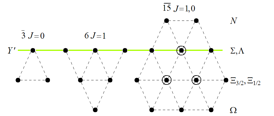
Figure 1: Rotational band of a soliton with one valence quark stripped off. Soliton spin corresponds to the isospin $T^{\prime}$ of states on the quantization line $Y^{\prime}=2/3$ (green thick line). We show three lowest allowed representations: antitriplet of spin 0, sextet of spin 1, and the lowest exotic representation $\overline{\mathbf{{15}}}$ of spin 1 or 0. On the right-hand side we display particle names used in the present paper.

In this picture, the allowed SU(3) representations have to contain states of $Y^{\prime}=2/3$, and these are $\overline{\boldsymbol{3}}$, $\boldsymbol{6}$, and exotic $\overline{\boldsymbol{15}}$ shown in Fig. 1. They correspond to the rotational excitations of the meson mean field, which is essentially the same as for light baryons. The corresponding wave function of the light sector is given in terms of the Wigner rotational $D(A)$ matrices [8]

$$\psi_{(\overline{\mathcal{R}}\,;\,-Y^{\prime}\,J\,J_{3})}^{(\mathcal{R\,};\,B)}(A)= \sqrt{\text{dim}(\mathcal{R})}\,(-)^{J_{3}-Y^{\prime}/2}$$

$$\times D_{(Y,\,T,\,T_{3})(Y^{\prime},\,J,\,-J_{3})}^{(\mathcal{R})\ast}(A)$$ (1)

where $\mathcal{R}$ denotes the SU(3) representation of the light sector, $B=(Y,T,T_{3})$ stands for the SU(3) quantum numbers of a baryon in question, and the second index of the $D$ function, $(Y^{\prime},J,-J_{3})$, corresponds to the soliton spin. $A(t)$ denotes relative configuration space – SU(3) group space rotation matrix.

The total wave function of a heavy baryon of spin $s$ is constructed by coupling (1) to a heavy quark spinor $\chi_{M}^{1/2}$ with a pertinent SU(2) Clebsch-Gordan coefficient,

$$\Psi_{B\,J\,s\,m}^{(\mathcal{R})}=\sum_{M,M_{J}}\chi_{M}^{1/2}\otimes\,\psi_{(\mathcal{\bar{R}};\,-Y^{\prime}\,J\,M_{J})}^{(\mathcal{R\,};\,B)}\;\left(\begin{array}[c]{cc}J&1/2\\ M_{J}&M\end{array}\right|\left.\begin{array}[c]{c}s\\ m\end{array}\right).$$ (2)

The rotational Hamiltonian takes the following form [36] in the chiral limit:

$$\mathcal{M}_{\mathcal{R}}= M_{\text{sol}}+\;\frac{1}{2I_{2}}\left[C_{2}(\mathcal{R})-T^{\prime}(T^{\prime}+1)-\frac{3}{4}Y^{\prime 2}\right]$$

$$+ \frac{1}{2I_{1}}T^{\prime}(T^{\prime}+1)$$ (3)

where $C_{2}(\mathcal{R})$ stands for the SU(3) Casimir operator. $M_{\text{sol}}\sim N_{c}$ denotes the classical soliton mass; $I_{1,2}\sim N_{c}$ are moments of inertia. All these parameters can, in principle, be calculated in some specific model. Here, we shall follow a so-called model-independent approach introduced in the context of the Skyrme model in Ref. [37], where all parameters are extracted from the experimental data [4].

The symmetry breaking Hamiltonian takes the following form [38]:

$$H_{\mathrm{{sb}}}=\alpha\,D_{88}^{(8)}+\beta\,\hat{Y}+\frac{\gamma}{\sqrt{3}}\sum_{i=1}^{3}D_{8i}^{(8)}\,\hat{J}_{i},$$ (4)

where $\alpha$, $\beta$, and $\gamma$ are proportional to the strange quark mass and are given in terms of the moments of inertia and the pion-nucleon sigma term. Their explicit form is not of interest to us, as we shall treat them as free parameters. It is however worth mentioning that $\alpha$ and $\beta$ are negative by construction, while $\gamma$ being phenomenologically negative is in fact given as a difference of two terms of the same order – see Eq. (4) in Ref [3]. Furthermore, $\alpha$ scales as $N_{c}$, and $\beta$ and $\gamma$ scale as $N_{c}^{0}$.

The soliton of $J=1$ can couple with the heavy quark to baryon spin $s=1/2$ or $s=3/2$. These states will be hyperfine split, and in order to take this into account, following [3], we supplement Hamiltonians (3) and (4) with the chromomagnetic interaction [3] expressed as:

$$H_{SQ}=\frac{2}{3}\frac{\varkappa}{m_{Q}}\hat{J}\cdot\hat{S}_{Q}$$ (5)

where $\varkappa$ denotes the anomalous chromomagnetic moment that is flavor independent. The operators ${\hat{J}}$ and ${\hat{S}}_{Q}$ represent the spin operators for the soliton and the heavy quark, respectively.

III Masses of heavy baryons

III.1 General formulas

As we can see from Fig. 1, the soliton in $\overline{\mathbf{{15}}}=(p=1,q=2)$ can be quantized both as spin $J=0$ and $1$ (remember that the isospin of the states on $Y^{\prime}=2/3$ line corresponds to spin). Next possible exotic representation is $\overline{\mathbf{15}}^{\prime}=(p=0,q=4)$ with spin $J=1$, which however, is heavier than $\overline{\mathbf{{15}}}$.

In order to estimate the masses of states in $\overline{\mathbf{{15}}}$ we shall use the general formula (3) for the rotational energy of the soliton. For the exotic representations in question we have

$$\mathcal{M}_{\overline{\mathbf{{15}}},J=0} = M_{\mathrm{{{sol}}}}+\frac{5}{2}\frac{1}{I_{2}}\,,$$

$$\mathcal{M}_{\overline{\mathbf{{15}}},J=1} = M_{\mathrm{{{sol}}}}+\frac{3}{2}\frac{1}{I_{2}}+\frac{1}{I_{1}}.$$ (6)

Interestingly, the mass difference

$$\Delta_{\overline{\mathbf{{15}}}} = \mathcal{M}_{\overline{\mathbf{{15}}},J=0}-\mathcal{M}_{\overline{\mathbf{{15}}},J=1}=\frac{1}{I_{2}}-\frac{1}{I_{1}}$$ (7)

is expected to be positive, since – from the estimates of the light sector [4, 8] – $I_{1}\sim(2.5\div 3)\times I_{2}$, which means that spin 1 soliton is lighter than the one of spin 0. One of the goals of the present analysis is to constrain these two parameters from the heavy sector alone. Indeed, solitons considered here are constructed from $N_{c}-1$ valence quarks, what may finally result in a change of the numerical values of $I_{1,2}$ as compared to the values extracted from the light sector [4].

The average multiplet masses take the following form:

$$M_{\overline{\mathbf{{3}}},J=0}^{Q} =m_{Q}+M_{\mathrm{{sol}}}+\frac{1}{2I_{2}},$$

$$M_{\mathbf{{6}},J=1}^{Q} =M_{\overline{\mathbf{{3}}}}^{Q}+\frac{1}{I_{1}},$$

$$M_{\overline{\boldsymbol{15}},J=1}^{Q} =M_{\mathbf{{6}}}^{Q}+\frac{1}{I_{2}},$$

$$M_{\overline{\boldsymbol{15}},J=0}^{Q} =M_{\mathbf{{6}}}^{Q}+\frac{2}{I_{2}}-\frac{1}{I_{1}}=M_{\overline{\boldsymbol{15}},J=1}^{Q}+\Delta_{\overline{\mathbf{{15}}}}.$$ (8)

Parameters $M_{\overline{\mathbf{{3}}}}^{Q}$ and $I_{1}$ can be extracted from the ground state nonexotic baryons [3]. In order to have some handle on $I_{2}$, and therefore on $\Delta_{\overline{\mathbf{{15}}}}$, we shall include now flavor symmetry breaking due to the mass difference between strange and non-strange quarks (4).

Calculating matrix elements of the symmetry breaking operator (4) between the collective wave functions (1) we obtain the following mass splittings for the ground state and excited baryons:

$$\left\langle H_{\text{sb}}\right\rangle_{\overline{\boldsymbol{3}},J=0} =\left(\frac{3}{8}{\alpha}+\beta\right)Y_{B}=\delta_{\overline{\mathbf{{3}}}}Y_{B}\,,$$

$$\left\langle H_{\text{sb}}\right\rangle_{{\boldsymbol{6}},J=1} =\left(\frac{3}{20}{\alpha}+\beta-\frac{3}{10}\gamma\right)Y_{B}=\delta_{\mathbf{{6}}}Y_{B}\,,$$

$$\left\langle H_{\text{sb}}\right\rangle_{\overline{\boldsymbol{15}},J=1} =\left(\beta+\frac{17}{144}(\alpha-2\gamma)\right)Y_{B}-(\alpha-2\gamma)$$

$$\times\left(\frac{2}{27}-\frac{1}{24}\left(T_{B}(T_{B}+1)-\frac{1}{4}Y_{B}^{2}\right)\right)\,,$$

$$\left\langle H_{\text{sb}}\right\rangle_{\overline{\boldsymbol{15}},J=0} =\left(\beta+\frac{1}{48}\alpha\right)Y_{B}$$

$$+\alpha\left(\frac{2}{9}-\frac{1}{8}\left(T_{B}(T_{B}+1)-\frac{1}{4}Y_{B}^{2}\right)\right)\,$$ (9)

where $Y_{B}$ and $T_{B}$ denote the hypercharge and the isospin of a given baryon, respectively. In the case of sextet and (${\overline{\boldsymbol{15}},J=1}$), the mass formula must be supplemented by the spin splitting Hamiltonian (5), leading to the following equations for baryon masses

$$M_{\mathcal{R}_{J},B,s}^{Q} =M_{\mathcal{R},J}^{Q}+\left\langle H_{\text{sb}}\right\rangle_{\mathcal{R},J}$$

$$+\delta_{J,1}\frac{\varkappa}{m_{Q}}\left\{\begin{array}[c]{ccc}-2/3&\text{for}&s=1/2\\ &&\\ +1/3&\text{for}&s=3/2\end{array}\right.$$ (13)

where $s$ denotes the spin of a given baryon, and $J$ is the soliton spin. It is worth to observe that the hyperfine splitting parameter $\varkappa/m_{Q}$ can estimated from the following mass differences:

$$M_{\mathcal{R}_{1},B,3/2}^{Q}\;-\;M_{\mathcal{R}_{1},B,1/2}^{Q}=\frac{\varkappa}{m_{Q}}.$$ (14)

It turns out that the mass formulas (9) for $\overline{\boldsymbol{15}}$ admit three Gell-Mann–Okubo (GMO) [39, 40] mass relations,

$$2N^{Q}+\Omega^{Q} =2\Lambda^{Q}+\Sigma^{Q},$$

$$N^{Q}+\Xi^{Q}_{3/2} =2\Sigma^{Q},$$

$$2N^{Q}+2\Xi^{Q}_{1/2} =3\Lambda^{Q}+\Sigma^{Q},$$ (15)

both in $J=1$ and $J=0$ multiplets. Although the mass formulas for both multiplets differ, the GMO mass relations are identical. It might be at the first sight surprising that for six isospin multiplets whose masses in the case of $\overline{\boldsymbol{15}}_{J=1}$ are parametrized by four parameters: $M^{Q}_{\overline{\boldsymbol{15}},J=1},\alpha,\beta$ and $\gamma$ we have three sum rules rather than two. The reason is that the splittings depend only on the combination $\alpha-2\gamma$. Relations (15) are linearly independent but not orthogonal. Furthermore, the following Guadagnini-type relation [33] is fulfilled:

$$\left[21N^{Q}-2\Lambda^{Q}+16\Sigma^{Q}-16\Xi^{Q}_{1/2}+11\Xi^{Q}_{3/2}-30\Omega^{Q}\right]_{\overline{\boldsymbol{15}}_{0}}$$

$$= \left[30N^{Q}+34\Lambda^{Q}-14\Sigma^{Q}+14\Xi^{Q}_{1/2}-58\Xi^{Q}_{3/2}-6\Omega^{Q}\right]_{\overline{\boldsymbol{15}}_{1}}.$$

(16)

Relation (16) has been constructed by demanding orthogonality to relations (15). It connects masses of different multiplets and therefore goes beyond the SU(3) symmetry.

III.2 Numerical estimates

Let us first consider masses of the nonexotic heavy baryons belonging to $\boldsymbol{\bar{3}}$ and $\boldsymbol{6}$ of SU(3). The average masses of these multiplets are given by Eqs. (8), in fact both for $Q=c$ and $b$,

$$M_{\overline{\mathbf{{3}}}}^{Q}=m_{Q}+M_{\mathrm{{sol}}}+\frac{1}{2I_{2}} =\left.2408.2\right|_{c}~{},~{}\left.5736.2\right|_{b}\,,$$

$$M_{\mathbf{{6}}}^{Q}=M_{\overline{\mathbf{{3}}}}^{Q}+\frac{1}{I_{1}} =\left.2579.7\right|_{c},~{}~{}\left.5906.5\right|_{b}$$ (17)

where the experimental values in MeV from Ref. [3] have been updated [41]. We can compute $I_{1}$ from the mass difference of these two multiplets (in MeV):

$$\frac{1}{I_{1}}=M_{\mathbf{6}}^{Q}-M_{\mathbf{\overline{3}}}^{Q}=\left.171.5\right|_{c}=\left.170.4\right|_{b}$$ (18)

Similarly we can compute heavy quark mass difference either from the mass difference of the bottom or charm antitriplets or sextets,

$$m_{b}-m_{c}= M_{\mathbf{6}}^{b}-M_{\mathbf{{6}}}^{c}=3327~{}\mathrm{{MeV},}$$

$$= M_{\mathbf{\overline{3}}}^{b}-M_{\mathbf{\overline{3}}}^{c}=3328~{}\mathrm{{MeV}.}$$ (19)

We consider perfect equality of splittings (18) regardless of $Q$ and the mass difference (19) regardless of the SU(3) representation, as a test of our model assumptions. Equalities (18) and (19) can be traced back to the fact that in the present model heavy baryon mass is simply a sum of a heavy quark mass and the rotational excitations of the soliton, see Eqs. (8), which are flavor-blind in the present approach. Moreover, the effects of SU(3) symmetry breaking are simply the same both for charm and bottom baryons, since they are solely due to the light quarks within the soliton.

Numerical value of $1/I_{1}$ from Eq. (18) should be compared with $1/I_{1}$ extracted from the light sector, which is equal to $\sim 155~{}{\rm MeV}$ [42]. This is consistent with the expectation that moments of inertia should be smaller in the case of heavy baryons, since the valence quark contributions to $I_{1,2}$ scales like $N_{\text{val}}$. In what follows, we shall assume $1/I_{1}=171$ MeV. Unfortunately, we cannot extract $I_{2}$ in a model independent way from the masses of the ground state multiplets. To this end, we have to use information from the mass splittings within different multiplets, including exotica.

In Ref. [3] the splitting parameters for $\overline{\boldsymbol{3}}$ and $\boldsymbol{6}$ have been extracted from experiment and read

$$\delta_{\overline{\mathbf{{3}}}}=\frac{3}{8}{\alpha}+\beta =-180~{}\mathrm{{MeV}\,,}$$

$$\delta_{\mathbf{{6}}}=\frac{3}{20}{\alpha}+\beta-\frac{3}{10}\gamma =-121~{}\mathrm{{MeV}\,.}$$ (20)

Numerical entries are taken as the average values from Eqs. (13) and (14) in Ref. [3].

In Ref. [4], two out of five excited $\Omega_{c}$ hyperons reported by the LHCb Collaboration in 2017 [9] have been interpreted as exotic states belonging to $(\overline{\mathbf{{15}}},J=1)$. Adding a heavy quark to the $J=1$ soliton results in two hyperfine split states (13) of spin $1/2$ and $3/2$ , namely $\Omega_{c}(3050)$ and $\Omega_{c}(3119)$, respectively. This splitting (14) is equal to $\varkappa/m_{c}=69$ MeV [3, 4]. $\Omega_{c}$ average mass before the spin splitting is

$$\overline{M}_{\Omega,(\overline{\mathbf{{15}}},J=1)}^{c}=3096\;\text{MeV.}$$ (21)

From Eqs. (6), (8) and (9) we obtain that

$$\overline{M}_{\Omega,(\overline{\mathbf{{15}}},J=1)}^{c} =M_{\mathbf{{6}}}^{c}+\frac{1}{I_{2}}-\frac{1}{6}\left(\alpha+8\beta-2\gamma\right)$$ (22)

Equating (21) with (22) together with Eqs. (20) gives three independent equations for four parameters $\alpha$, $\beta$, $\gamma$ and $1/I_{2}$. We solve them in function of $1/I_{2}$ and constrain parameter $1/I_{2}$ to the region where both $\alpha$ and $\beta$ are negative. The result is plotted in Fig. 2.

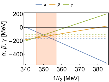
Figure 2: Parameters $\alpha$, $\beta$, and $\gamma$ plotted in terms of the inverse moment of inertia $1/I_{2}$. Expectations from the light sector are shown as dashed lines.

We see from Fig. 2 that the allowed range (i.e., the range where $\alpha,\beta<0$) for the second moment of inertia is $342~{}\mathrm{{MeV}<1/I_{2}<380}$ MeV. However, all model calculations and fits to the light sector suggest that also parameter $\gamma$ should be negative (see, e.g., Ref. [24]); then the allowed range for $1/I_{2}$ is further constrained to $1/I_{2}<363$ MeV. The most probable value of $1/I_{2}$ is around 351 MeV, where all splitting parameters are negative and of the same order. Indeed, from fits to the light sector one obtains [3] $\alpha=-255~{}\mathrm{{MeV},\;\;\;\beta=-140~{}{MeV},\;\;\;\gamma=-101~{}{MeV}}$. However, as explained in Ref. [3], the parameter $\alpha$ scales linearly with the number of valence quarks, $N_{\mathrm{{val}}}$, whereas parameters $\beta$ and $\gamma$ are in the first approximation independent of $N_{\mathrm{{val}}}$, because they are equal to the ratios of quantities that scale like $N_{\mathrm{{val}}}$. This means that in the heavy baryon sector, we expect $\alpha\rightarrow 2/3\times(-255)=-170$ MeV. From our fits for $1/I_{2}\simeq 351$ MeV, we obtain $\alpha\simeq-110$ MeV, $\beta\simeq-139$ MeV and $\gamma\simeq-114$ MeV. Here only $\alpha$ is substantially different from the light sector estimate. This is shown in more detail in Fig. 2 where model expectations from the light sector are shown as dashed lines. In what follows, we shall discuss the sensitivity of heavy pentaquark masses to the variation of $1/I_{2}$ within the limits $\pm 5$ MeV around 351 MeV. This is shown as a light-orange band in Fig. 2.

Finally, let us observe that assuming $1/I_{2}=351$ MeV and taking $1/I_{1}$ from Eq. (18), we obtain that $(\overline{\mathbf{{15}}},J=0)$ multiplet is heavier from $(\overline{\mathbf{{15}}},J=1)$ multiplet on average by approximately $180$ MeV. We have, therefore,

$$M_{\overline{\boldsymbol{15}},J=1}^{c} \simeq 2931\;\text{MeV},$$

$$M_{\overline{\boldsymbol{15}},J=0}^{c} \simeq 3111\;\text{MeV.}$$ (23)

At this point, we can estimate the average mass of the next exotic representation $(\overline{\boldsymbol{15}}^{\prime}=(p=0,q=4),J=1)$ to be approximately 3633 MeV, which is indeed substantially heavier than $\overline{\boldsymbol{15}}$.

$\overline{\boldsymbol{15}}$	$J=1$		$J=0$
	$s=1/2$	$s=3/2$	$s=1/2$
$N^{c}$	2644–2692	2713–2761	2819–2884
$\Lambda^{c}$	2772–2812	2841–2881	2981–3001
$\Sigma^{c}$	2795–2810	2864–2879	2993–3043
$\Xi_{1/2}^{c}$	2911–2931	2980–3000	3148–3138
$\Xi_{3/2}^{c}$	2945–2927	3014–2996	3167–3202
$\Omega^{c}$	3050	3119	3316–3276

Table 1: Mass predictions in MeV for exotic $\overline{\boldsymbol{15}}$. Two $\Omega^{c}$ states are taken as input.

In Fig. 3 and in Tab. 1 we show the results for $\overline{\boldsymbol{15}}$ masses both for $J=$ and $J=0$. Our predictions for $J=1$ multiplets are in agreement with Ref. [4], where parameters $\alpha$, $\beta$, and $\gamma$ have been estimated from the light sector alone.

It is interesting to compare our phenomenological results with model calculations of Ref. [24]. Using modified chiral fields, they obtain $1/I_{2}\simeq 380$ MeV, i.e. above the upper edge of our allowed window shown in Fig 2. This is the reason why their mass predictions are higher than in the present work. Their parameters $\alpha$ and $\beta$ are similar to ours, although $\alpha$ is a bit smaller and $\beta$ a bit larger. On the other hand, $\gamma$ is much larger than in our case, but still negative. The latter explains why their value of $\delta_{\boldsymbol{6}}$ undershoots experiment (20) by $\sim 15\%$. The values of their parameters are, however, consistent with the dependence on $1/I_{2}$ displayed in Fig 2. It should be stressed that the calculations in Ref. [24] have been done for one particular choice of chiral fields, namely for the pseudoscalars only. Nevertheless, their results support our initial conjecture that for $N_{c}=3$, we expect that numerical values of model parameters differ depending of the number of quarks in the soliton valence level.

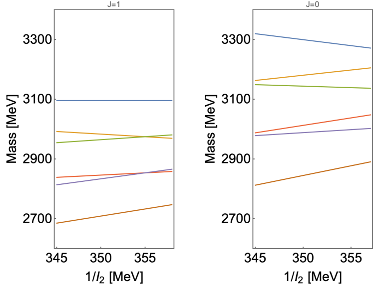
Figure 3: Spectra of exotic charm multiplets ${\overline{\boldsymbol{15}},J=1}$ (left) and $J=0$ (right) in terms of the inverse moment of inertia $1/I_{2}$.

IV Decays

IV.1 General formulas

To calculate the decays of heavy baryons, one has to sandwich the corresponding decay operator between the wave functions (2). Following Ref. [8], we use in this paper the decay operator describing the emission of a $p-$wave pseudoscalar meson $\varphi$, which has been obtained via the Goldberger-Treiman relation from the collective weak current [5],

$$\mathcal{O}_{\varphi} =\frac{1}{2F_{\varphi}}\left[-\tilde{a}_{1}D_{\varphi\,i}^{(8)}-a_{2}\,d_{ibc}D_{\varphi\,b}^{(8)}\hat{J}_{c}-a_{3}\frac{1}{\sqrt{3}}D_{\varphi\,8}^{(8)}\hat{J}_{i}\right]\,p_{i}.$$

(24)

Constants $a_{1,2,3}$ that enter Eq. (24) have been extracted from the semileptonic decays of the baryon octet in Ref. [43]:

$$a_{1}\simeq-3.509\,,\;a_{2}\simeq 3.437\,,\;a_{3}\simeq 0.604\,.$$ (25)

However, due to the fact that $a_{1}$ scales as $N_{\rm val}$, it has been shown in Ref. [5] that in the heavy quark sector $a_{1}$ has to be replaced by

$$a_{1}\rightarrow\tilde{a}_{1}=-2.1596.$$ (26)

With this replacement, all decays of charm and bottom sextet and of two exotic $\Omega_{c}$’s have been successfully described by the present model [5]. For the decay constants $F_{\varphi}$, we have adopted the convention in which $F_{\pi}=93$ MeV and $F_{K}=F_{\eta}=1.2\,F_{\pi}=112$ MeV.

We are considering decays $B_{1}\rightarrow B_{2}+\varphi$, where $M_{1,2}$ denote masses of the initial and final baryons respectively, and $p_{i}$ is the c.m. momentum of the outgoing meson of mass $m$ [5, 8]:

$$\left|\vec{p}\,\right|=p=\frac{\sqrt{(M_{1}^{2}-(M_{2}+m)^{2})(M_{1}^{2}-(M_{2}-m)^{2})}}{2M_{1}}$$ (27)

The decay width is related to the matrix element of $\mathcal{O}_{\varphi}$ squared, summed over the final isospin (but not spin) and averaged over the initial spin and isospin denoted as $\overline{\left[\ldots\right]^{2}}$; see the Appendix of Ref. [8] and Erratum of Ref. [5] for the details of the corresponding calculations,

$$\Gamma_{B_{1}\rightarrow B_{2}+\varphi}=\frac{1}{2\pi}\overline{\left\langle B_{2}\left|\mathcal{O}_{\varphi}\right|B_{1}\right\rangle^{2}}\,\frac{M_{2}}{M_{1}}p.$$ (28)

Here factor $M_{2}/M_{1}$, used already in Ref. [5], is the same as in heavy baryon chiral perturbation theory (HBChPT); see e.g. Ref. [44].

$\overline{\boldsymbol{15}}_{J=1}$	$\boldsymbol{6}_{J=1}$	allowed
$\Omega^{c}$	$\Omega^{c}+\pi$	yes
	$\Xi^{c}+\overline{K}$	yes∗
$\Xi^{c}_{3/2,1/2}$	$\Xi^{c}+\pi$	yes
	$\Sigma^{c}+\overline{K}$	yes∗
$\Xi^{c}_{1/2}$	$\Omega^{c}+{K}$	no
	$\Xi^{c}+\eta$	no
$\Sigma^{c},\,\Lambda^{c}$	$\Xi^{c}+K$	no
	$\Sigma^{c}+\pi$	yes
$\Sigma^{c}$	$\Sigma^{c}+\eta$	no
$N^{c}$	$\Sigma^{c}+{K}$	no

Table 2: Decays of $\overline{\boldsymbol{15}}_{J=1}$ to $\boldsymbol{6}_{J=1}$. (^∗only $s=3/2\rightarrow s=1/2$).

$\overline{\boldsymbol{15}}_{J=1}$	${\overline{\boldsymbol{3}}}_{J=0}$	allowed
$\Omega^{c}$	$\Xi^{c}+\overline{K}$	yes
$\Xi^{c}_{3/2,1/2}$	$\Xi^{c}+\pi$	yes
$\Xi^{c}_{1/2}$	$\Xi^{c}+\eta$	no†
	$\Lambda^{c}+\overline{K}$	yes
$\Sigma^{c}$	$\Xi^{c}+{K}$	no
	$\Lambda^{c}+\pi$	yes
$\Lambda^{c}$	$\Lambda^{c}+\eta$	yes∗
	$\Xi^{c}+{K}$	no
$N^{c}$	$\Lambda^{c}+{K}$	no

Table 3: Decays of $\overline{\boldsymbol{15}}_{J=1}$ to ${\overline{\boldsymbol{3}}}_{J=0}$. (^∗only $s=3/2$,  ^† $s=3/2$ at the threshold).

Because operator $\mathcal{O}_{\varphi}$ does not depend on the heavy quark spin, it is only the soliton that decays by emitting a pseudoscalar meson. Heavy quark acts as a spectator of the decaying soliton. Since the decay occurs in the $p-$wave, the final soliton spin has to couple with meson angular momentum $l=1$ to the spin of the initial state soliton. Decays with heavy quark spin flip are suppressed by $1/m_{Q}$ and are not considered here. Mesons are in the SU(3) octet and therefore the following decays are possible:

$$\overline{\boldsymbol{15}}_{J=1} \rightarrow\boldsymbol{6}_{J=1},\overline{\,\boldsymbol{3}}_{J=0},$$

$$\overline{\boldsymbol{15}}_{J=0} \rightarrow\overline{\boldsymbol{15}}_{J=1},\boldsymbol{6}_{J=1}.$$ (29)

Direct decays of $\overline{\boldsymbol{15}}_{J=0}$ to the ground state antitriplet are suppressed. In Tables 3 – 6, we list all decays that are allowed by the quantum numbers. Taking into account mass estimates from the previous section, we find that some of these decays are excluded by the energy conservation (column 3). Furthermore, in Tab. 6, we list all possible decays of exotic $\overline{\boldsymbol{15}}$ to the ground state baryons and heavy mesons (calculation of which is beyond the scope of the present paper).

$\overline{\boldsymbol{15}}_{J=0}$	$\overline{\boldsymbol{15}}_{J=1}$	allowed
$\Omega^{c}$	$\Omega^{c}+\pi$	yes
	$\Omega^{c}+\eta$	no
	$\Xi^{c}_{3/2,1/2}+\overline{K}$	no
$\Xi^{c}_{3/2,1/2}$	$\Omega^{c}+{K}$	no
	$\Xi^{c}_{3/2,1/2}+\pi$	yes∗
	$\Sigma^{c}+\overline{K}$	no
$\Xi^{c}_{1/2}$	$\Xi^{c}_{1/2}+\eta$	no
	$\Lambda^{c}+\overline{K}$	no
$\Xi^{c}_{3/2}$	$\Xi^{c}_{3/2}+\eta$	no
$\Sigma^{c}$	$\Xi^{c}_{3/2,1/2}+K$	no
	$\Lambda^{c}+\pi$	yes
	$\Sigma^{c}+\pi$	yes
	$\Sigma^{c}+\eta$	no
	$N^{c}+\overline{K}$	no
$\Lambda^{c}$	$\Xi^{c}_{1/2}+K$	no
	$\Lambda^{c}+\eta$	no
	$\Sigma^{c}+\pi$	yes†
	$N^{c}+\overline{K}$	no
$N^{c}$	$\Sigma^{c}+{K}$	no
	$\Lambda^{c}+{K}$	no
	$N^{c}+\pi$	yes#
	$N^{c}+\eta$	no

Table 4: Decays of $\overline{\boldsymbol{15}}_{J=0}$ to $\overline{\boldsymbol{15}}_{J=1}$. (${}^{*}~{}\Xi_{1/2}\rightarrow\Xi_{3/2}(s=3/2)$ below the threshold,  ${}^{\dagger}~{}s=1/2\rightarrow s=3/2$ below the threshold,  ^# only $s=3/2\rightarrow s=1/2$ allowed).

$\overline{\boldsymbol{15}}_{J=0}$	$\boldsymbol{6}_{J=1}$	allowed
$\Omega^{c}$	$\Omega^{c}+\pi$	yes
	$\Xi^{c}+\overline{K}$	yes
$\Xi^{c}_{3/2,1/2}$	$\Xi^{c}+\pi$	yes
	$\Sigma^{c}+\overline{K}$	yes
$\Xi^{c}_{1/2}$	$\Omega^{c}+{K}$	no
	$\Xi^{c}+\eta$	no∗
$\Sigma^{c},\Lambda$	$\Xi+K$	no
	$\Sigma^{c}+\pi$	yes
$\Sigma^{c}$	$\Sigma^{c}+\eta$	yes†
$N^{c}$	$\Sigma^{c}+{K}$	no

Table 5: Decays of $\overline{\boldsymbol{15}}_{J=0}$ to $\boldsymbol{6}_{J=1}$. (^∗decay to $s=1/2$ at the threshold, ^†only to $s=1/2$).

$\overline{\boldsymbol{15}}$	final	$J=1$	$J=0$
$\Omega^{c}$	$\Xi+D$	no	yes
$\Xi^{c}_{3/2}$	$\Sigma+D$	no	yes
$\Xi^{c}_{1/2}$	$\Xi+D_{s}$	no	no
	$\Lambda+D$	no	yes
	$\Sigma+D$	no	yes
$\Sigma^{c}$	$\Sigma+D_{s}$	no	no
	$N+D$	yes∗	yes
$\Lambda^{c}$	$\Lambda+D_{s}$	no	no
	$N+D$	yes∗	yes
$N^{c}$	$N+D_{s}$	no	no

Table 6: Decays of $\overline{\boldsymbol{15}}_{J=1,0}$ to the ground state octet baryons and $D$ mesons (^∗only $s=3/2$).

Already at this point we can draw interesting conclusions. For $\overline{\boldsymbol{15}}_{J=1}$, we have ten allowed decays of the type (29) and for $\overline{\boldsymbol{15}}_{J=0}$ twelve. Interestingly, the lightest members of both multiplets, namely $N_{\overline{\boldsymbol{15}}}$ are stable against two body strong interactions. Except for $N_{\overline{\boldsymbol{15}}}$, all members of $J=0$ multiplet have open channels to the decays to heavy mesons.

After averaging over the initial spin and isospin and summing over the final isospin and over final spin third component $m_{2}$, we arrive at the following expressions for the decay widths:

$$\Gamma_{B_{1}\rightarrow B_{2}+\varphi}= \frac{p^{3}}{24\pi F_{\varphi}^{2}}\frac{M_{2}}{M_{1}}\,\frac{\dim\mathcal{R}_{2}}{\dim\overline{\boldsymbol{15}}}\;\gamma_{J_{1}\rightarrow J_{2}}(s_{1}\rightarrow s_{2})$$

$$\times \left(\sum_{\mu}{\mathcal{G}}_{\overline{\boldsymbol{15}}_{J_{1}}\rightarrow\mathcal{R}_{2}}^{(\mu)}\left[\begin{array}[c]{cc}8&\mathcal{R}_{2}\\ \varphi&B_{2}\end{array}\right|\left.\begin{array}[c]{c}\overline{\boldsymbol{15}}_{\mu}\\ B_{1}\end{array}\right]\right)^{2}\,.$$ (34)

Here the square bracket stands for the pertinent SU(3) isoscalar factor coupling meson and baryon in a final state to the baryon in the initial state and ${\mathcal{G}}^{(\mu)}_{\overline{\boldsymbol{15}}_{J_{1}}\rightarrow\mathcal{R}_{2}}$ is the decay coupling (see below). The sum over $\mu$ is relevant only for $\mathcal{R}_{2}=\overline{\boldsymbol{15}}$ in the final state. Here, we adopt the de Swart conventions for the SU(3) phase factors [45] and label the representations as in the numerical code of Ref. [46]. Factors $\gamma$ take care of the spin dependence for the soliton angular momenta $J=1$ or 0 (see Erratum in Ref. [5]):

$$\gamma_{1\rightarrow 1}(1/2\rightarrow 1/2)=2/3, \qquad\gamma_{1\rightarrow 1}(1/2\rightarrow 3/2)=1/3,$$

$$\gamma_{1\rightarrow 1}(3/2\rightarrow 1/2)=1/6, \qquad\gamma_{1\rightarrow 1}(3/2\rightarrow 3/2)=5/6,$$

$$\gamma_{0\rightarrow 1}(1/2\rightarrow 1/2)=1/3, \qquad\gamma_{0\rightarrow 1}(1/2\rightarrow 3/2)=2/3,$$

$$\gamma_{1\rightarrow 0}(1/2\rightarrow 1/2)=1,~{}~{}\, \qquad\gamma_{1\rightarrow 0}(3/2\rightarrow 1/2)=1.$$ (35)

Note that

$$\sum_{s_{2}}\gamma_{J_{1}\rightarrow J_{2}}(s_{1}\rightarrow s_{2})=1\,.$$ (36)

Finally, the decay constants read

$${\mathcal{G}}_{{\overline{\boldsymbol{15}}_{1}}\rightarrow{\overline{\boldsymbol{3}}}_{0}} =\sqrt{\frac{1}{2}}\left(-\tilde{a}_{1}-\frac{1}{2}a_{2}\right)=0.312\,,$$

$${\mathcal{G}}_{\overline{\boldsymbol{15}}_{1}\rightarrow{\boldsymbol{6}}_{1}} =-\sqrt{\frac{1}{3}}\left(-\tilde{a}_{1}-\frac{1}{2}a_{2}-a_{3}\right)=0.094\,,$$

$${\mathcal{G}}_{\overline{\boldsymbol{15}}_{0}\rightarrow{\boldsymbol{6}}_{1}} =\frac{1}{2}\left(-\tilde{a}_{1}-\frac{3}{2}a_{2}\right)=-1.498\,,$$

$${\mathcal{G}}^{(\mu=1)}_{{\overline{\boldsymbol{15}}_{0}}\rightarrow{\overline{\boldsymbol{15}}}_{1}} =\sqrt{\frac{1}{366}}\left(-\tilde{a}_{1}+\frac{41}{2}a_{2}\right)=3.796\,,$$

$${\mathcal{G}}^{(\mu=2)}_{{\overline{\boldsymbol{15}}_{0}}\rightarrow{\overline{\boldsymbol{15}}}_{1}} =-\sqrt{\frac{81}{122}}\left(-\tilde{a}_{1}+\frac{1}{6}a_{2}\right)=-2.226\,.$$ (37)

To compute the numerical values, we have used Eqs. (25) and (26). We see from Eqs. (37) that decay constants of $(\overline{\boldsymbol{15}},J=1)$ are very small; in fact they vanish in the large $N_{c}$ limit [47]. On the contrary, decay constants of $(\overline{\boldsymbol{15}},J=0)$ are almost an order of magnitude larger, so we expect the corresponding decay widths to be large (furthermore, the phase space factor $p^{3}$ will be larger than in the $J=1$ case).

IV.2 Numerical estimates

Numerical estimates of the decay widths, assuming central values for baryon masses from Table 1, are listed in Tables 7 and 8. One should note that these widths are pure predictions based on the light sector values of the decay parameters, except for rescaling (26).

Decay widths of the $\Omega^{c}$ states from $\overline{\boldsymbol{15}}_{J=1}$, $\Gamma=0.43$ MeV and 0.98 MeV have been already computed in Ref. [5] and agree within uncertainties with experimental widths equal to $0.8\pm 0.2\pm 0.1$ MeV and $1.1\pm 0.8\pm 0.4$ MeV, respectively [9]. Our present results also agree with initial estimates of the decay widths of two exotic $\Xi^{c}_{3/2}$ states given in Ref. [5] (note that here we have slightly different masses).

We see from Table 7 that all states in $\overline{\boldsymbol{15}}_{J=1}$, have very small widths, in most cases not exceeding 1 MeV. For almost all states in $\overline{\boldsymbol{15}}_{J=1}$, decay channels to light baryons and heavy mesons are closed (except for $\Sigma^{c}$ and $\Lambda^{c}$ of spin $s=3/2$, which are at the threshold). We therefore conclude that exotic charm pentaquarks from $\overline{\boldsymbol{15}}_{J=1}$ can be found only in dedicated searches in high resolution experiments. One should also observe that, as already shown in Tables 3 and 3, that the lightest member of $\overline{\boldsymbol{15}}_{J=1}$, namely the nucleonlike pentaquark, is stable with respect to two body strong decays.

decay		$\Gamma$ [MeV]
$B_{1}$	$B_{2}+\varphi$	$s_{2}=\frac{1}{2}$	$s_{2}=\frac{3}{2}$	$\Sigma_{s_{2}}$
$\Omega^{c}({\boldsymbol{\overline{15}}}_{1}^{1/2})$	$\Xi^{c}({\overline{\boldsymbol{3}}}_{0})+\overline{K}$	0.349	– – –	0.349
	$\Omega^{c}({\boldsymbol{6}}_{1})+\pi$	0.062	0.015	0.077
	total			0.425
	$\Xi^{c}({\overline{\boldsymbol{3}}}_{0})+\overline{K}$	0.875	– – –	0.875
$\Omega^{c}({\boldsymbol{\overline{15}}}_{1}^{3/2})$	$\Omega^{c}({\boldsymbol{6}}_{1})+\pi$	0.027	0.077	0.104
	$\Xi^{c}({{\boldsymbol{6}}}_{1})+\overline{K}$	0.002	– – –	0.002
	total			0.981
$\Xi^{c}_{3/2}({\overline{\boldsymbol{15}}}_{1}^{1/2})$	$\Xi^{c}({\overline{\boldsymbol{3}}}_{0})+\pi$	1.636 – 1.830	– – –	1.636 – 1.830
	$\Xi^{c}({\boldsymbol{6}}_{1})+\pi$	0.029 –0.035	0.007 – 0.009	0.036 – 0.043
	total			1.672 – 1.874
	$\Xi^{c}({\overline{\boldsymbol{3}}}_{0})+\pi$	2.447 – 2.687	– – –	2.447 – 2.687
$\Xi^{c}_{3/2}({\overline{\boldsymbol{15}}}_{1}^{3/2})$	$\Xi^{c}({\boldsymbol{6}}_{1})+\pi$	0.013 – 0.015	0.037 – 0.044	0.050 – 0.058
	$\Sigma^{c}({\boldsymbol{6}}_{1})+\overline{K}$	0.003 – 0.005	$\approx$ 0	0.003 – 0.005
	total			2.497 – 2.751
	$\Xi^{c}({\boldsymbol{3}}_{0})+\pi$	0.092 – 0.105	– – –	0.092 – 0.105
$\Xi^{c}_{1/2}({\overline{\boldsymbol{15}}}_{1}^{1/2})$	$\Lambda^{c}({\overline{\boldsymbol{3}}}_{0})+\overline{K}$	0.239 – 0.299	– – –	0.239 – 0.299
	$\Xi^{c}({\overline{\boldsymbol{6}}}_{1})+\pi$	0.039 – 0.048	0.009 – 0.011	0.048 – 0.059
	total			0.379 – 0.463
	$\Xi^{c}({\boldsymbol{3}}_{0})+\pi$	0.140 – 0.156	– – –	0.140 – 0.156
$\Xi^{c}_{1/2}({\overline{\boldsymbol{15}}}_{1}^{3/2})$	$\Lambda^{c}({\overline{\boldsymbol{3}}}_{0})+\overline{K}$	0.468 – 0.546	– – –	0.468 – 0.546
	$\Xi^{c}({\overline{\boldsymbol{6}}}_{1})+\pi$	0.018 – 0.021	0.049 – 0.060	0.068 – 0.081
	$\Sigma^{c}({\boldsymbol{6}}_{1})+\overline{K}$	$\approx$ 0	– – –	$\approx$ 0
	total			0.676 – 0.783
$\Sigma^{c}({\overline{\boldsymbol{15}}}_{1}^{1/2})$	$\Lambda^{c}({\overline{\boldsymbol{3}}}_{0})+\pi$	1.073 – 1.165	– – –	1.073 – 1.165
	$\Sigma^{c}({\boldsymbol{6}}_{1})+\pi$	0.027 – 0.031	0.006 – 0.008	0.033 – 0.039
	total			1.107 – 1.203
$\Sigma^{c}({\overline{\boldsymbol{15}}}_{1}^{3/2})$	$\Lambda^{c}({\overline{\boldsymbol{3}}}_{0})+\pi$	1.525 – 1.635	– – –	1.525 – 1.635
	$\Sigma^{c}({\boldsymbol{6}}_{1})+\pi$	0.012 – 0.013	0.035 – 0.040	0.047 – 0.054
	total			1.572 – 1.688
$\Lambda^{c}({\overline{\boldsymbol{15}}}_{1}^{1/2})$	$\Sigma^{c}({\boldsymbol{6}}_{1})+\pi$	0.016 – 0.023	0.004 –0.006	0.019 – 0.030
	total			0.019 – 0.030
$\Lambda^{c}({\overline{\boldsymbol{15}}}_{1}^{3/2})$	$\Lambda^{c}({\overline{\boldsymbol{3}}}_{0})+\eta$	0.006 – 0.108	– – –	0.006 –0.108
	$\Sigma^{c}({\boldsymbol{6}}_{1})+\pi$	0.008 – 0.010	0.021 – 0.031	0.028 – 0.041
	total			0.034 – 0.149

Table 7: Decay widths of exotic pentaquarks in the SU(3) representation $\overline{\boldsymbol{15}}$ and $J=1$. Uncertainties correspond to the mass ranges from Table 1 (two $\Omega^{c}$ states are used as the input; therefore, their masses and decays widths are not subject to such uncertainties).

decay		$\Gamma$ [MeV]
$B_{1}$	$B_{2}+\varphi$	$s_{2}=\frac{1}{2}$	$s_{2}=\frac{3}{2}$	$\Sigma_{s_{2}}$
	$\Omega^{c}({\boldsymbol{6}}_{1})+\pi$	34.18 – 41.02	47.93 – 59.38	82.10 – 100.39
$\Omega^{c}({\overline{\boldsymbol{15}}}_{0})$	$\Xi_{1/2}({{\boldsymbol{6}}}_{1})+\overline{K}$	7.14 – 9.53	7.5 – 11.31	14.63 – 20.84
	$\Omega^{c}({\overline{\boldsymbol{15}}}_{1})+\pi$	1.49 – 2.97	0.23 – 1.48	1.72 – 4.46
	total			98.46 – 125.68
	$\Xi^{c}({\boldsymbol{6}}_{1})+\pi$	17.52 – 20.48	25.04 – 30.06	42.56 –50.55
$\Xi^{c}_{3/2}({\overline{\boldsymbol{15}}}_{0})$	$\Sigma^{c}({\boldsymbol{6}}_{1})+\overline{K}$	15.50 – 19.7	17.99 – 24.90	33.49 – 44.60
	$\Xi^{c}_{3/2}({\overline{\boldsymbol{15}}}_{1})+\pi$	22.83 – 56.04	2.65 – 31.53	25.48 – 87.57
	$\Xi^{c}_{1/2}({\overline{\boldsymbol{15}}}_{1})+\pi$	2.66 – 6.11	0.67 – 4.04	3.33 – 10.16
	total			104.86 – 192.89
	$\Xi^{c}({\boldsymbol{6}}_{1})+\pi$	23.83 – 25.01	33.21 – 35.19	57.04 – 60.21
$\Xi^{c}_{1/2}({\overline{\boldsymbol{15}}}_{0})$	$\Sigma^{c}({\boldsymbol{6}}_{1})+\overline{K}$	0.77 – 0.84	0.81 – 0.91	1.58 – 1.75
	$\Xi^{c}_{3/2}({\overline{\boldsymbol{15}}}_{1})+\pi$	1.93 – 3.95	0 – 0.42	1.93 – 4.37
	$\Xi^{c}_{1/2}({\overline{\boldsymbol{15}}}_{1})+\pi$	0.09 – 0.17	0 – 0.05	0.09 – 0.22
	total			60.64 – 66.55
	$\Sigma^{c}({\boldsymbol{6}}_{1})+\pi$	13.38 – 17.08	18.83 – 25.06	32.21 – 42.14
$\Sigma^{c}({\overline{\boldsymbol{15}}}_{0})$	$\Sigma^{c}({\boldsymbol{6}}_{1})+\eta$	0 – 0.95	– – –	0 – 0.95
	$\Sigma^{c}({\overline{\boldsymbol{15}}}_{1})+\pi$	7.31 – 34.90	0 – 12.55	7.31 – 47.45
	$\Lambda^{c}({\overline{\boldsymbol{15}}}_{1})+\pi$	0.95 – 6.95	0 – 3.74	0.95 – 10.68
	total			40.46 – 101.23
$\Lambda^{c}({\overline{\boldsymbol{15}}}_{0})$	$\Sigma^{c}({\boldsymbol{6}}_{1})+\pi$	9.42 – 10.46	13.10 – 14.82	22.53 – 25.27
	$\Sigma^{c}({\overline{\boldsymbol{15}}}_{1})+\pi$	1.84 – 6.21	– – –	1.84 – 6.21
	total			28.74 – 31.48
$N^{c}({\overline{\boldsymbol{15}}}_{0})$	$N^{c}({\overline{\boldsymbol{15}}}_{1})+\pi$	0 – 34.47	0 – 9.98	0 – 44.45
	total			0 – 44.45

Table 8: Decay widths of exotic pentaquarks in the SU(3) representation $\overline{\boldsymbol{15}}$ and $J=0$. Uncertainties correspond to the mass ranges from Table 1.

The situation is completely different in the case of $\overline{\boldsymbol{15}}_{J=0}$ listed in Table 8. Here all decay widths are within 30 – 140 MeV range. The only exception is again the lightest nucleonlike pentaquark, which however, can decay only to the $N^{c}$ state in $\overline{\boldsymbol{15}}_{J=1}$, which is semistable. Furthermore, all states in $\overline{\boldsymbol{15}}_{J=0}$ (except for $N^{c}$) have at least one open channel to the decays to light baryons and heavy mesons. We are not able to compute these widths within the present approach. However, since the available phase space is comparable to the decays listed in Tab. 8, we may expect that the total decay widths will double with respect to the estimates given in Tab. 8.

One should also note, that all decays of $\overline{\boldsymbol{15}}_{J=0}$ lead to either $\boldsymbol{6}$ or $\overline{\boldsymbol{15}}_{J=1}$, which decay further to $\boldsymbol{6}$ and $\overline{\boldsymbol{3}}$.

We conclude therefore, that pentaquarks from $\overline{\boldsymbol{15}}_{J=0}$ multiplet are very wide and may be interpreted as a background, rather than as a signal. Therefore, they could have been missed in general purpose experiments.

V Summary and conclusions

In the present paper we have studied the consequences of possible existence of heavy pentaquark SU(3) multiplets. Charmed pentaquarks have been evoked to explain small widths of two excited $\Omega^{c}$ states [4] announced in 2017 by the LHCb Collaboration at CERN [9]. Such interpretation requires, however, the existence of many other exotic and cryptoexotic charm baryons that have not been observed experimentally.

For the present study we have employed the $\chi$QSM estimating its parameters from the heavy baryon spectra. Therefore strictly speaking, we have not tested the dynamics of the model, but rather the underlying hedgehog SU(3) symmetry. Such symmetry leads to the sum rules (15) analogous to the Gell-Mann–Okubo mass relations [39, 40] and to one Guadagnini-type [33] relation (16).

We presented numerical support for the model mass formulas (8), (9) and (13). Next, we extracted model parameters from the heavy baryon spectra alone, and from the positivity of splitting parameters $\alpha,~{}\beta$, and $\gamma$ (4). We obtained mass ranges of the charm pentaquarks with uncertainties of the order $\sim 50$ MeV. Of course this is a conservative estimate, as the model itself is to large extent semiquantitave.

Finally, we computed the decay widths. Here, predictions for known experimentally ground state charm baryons as well as for two exotic $\Omega^{c}$ states, are very accurate [5]. We therefore have confidence in our predictions for the remaining exotic states.

We have found that pentaquarks belonging to the $\overline{\boldsymbol{15}}_{J=1}$ SU(3) multiplet are very narrow having widths of the order of $\sim 1$ MeV, while the remaining states from the $\overline{\boldsymbol{15}}_{J=0}$ SU(3) multiplet are wide, in most cases of the order of $\sim 100$ MeV or more. Moreover, all these decays lead to the unstable resonances; therefore, the identification of exotica requires dedicated experiments. Multipurpose searches could easily miss narrow or wide exotic states.

References

- [1] H. Y. Cheng, Chin. J. Phys. 78, 324-362 (2022) [arXiv:2109.01216 [hep-ph]].
- [2] P.A. Zyla et al. (Particle Data Group), Prog. Theor. Exp. Phys. 083C01 (2020) and 2021 update.
- [3] G. S. Yang, H.-Ch. Kim, M. V. Polyakov and M. Praszalowicz, Phys. Rev. D 94, 071502 (2016).
- [4] H. C. Kim, M. V. Polyakov and M. Praszałowicz, Phys. Rev. D 96 (2017) no.1, 014009 doi:10.1103/PhysRevD.96.014009 [arXiv:1704.04082 [hep-ph]].
- [5] H. C. Kim, M. V. Polyakov, M. Praszalowicz and G. S. Yang, Phys. Rev. D 96, no.9, 094021 (2017) [erratum: Phys. Rev. D 97, no.3, 039901 (2018)] doi:10.1103/PhysRevD.96.094021 [arXiv:1709.04927 [hep-ph]].
- [6] M. V. Polyakov and M. Praszalowicz, Phys. Rev. D 105, 094004 (2022) doi:10.1103/PhysRevD.105.094004 [arXiv:2201.07293 [hep-ph]].
- [7] M. Praszalowicz, Phys. Lett. B 575, 234-241 (2003) doi:10.1016/j.physletb.2003.09.049 [arXiv:hep-ph/0308114 [hep-ph]].
- [8] D. Diakonov, V. Petrov and M. V. Polyakov, Z. Phys. A 359, 305-314 (1997) doi:10.1007/s002180050406 [arXiv:hep-ph/9703373 [hep-ph]].
- [9] R. Aaij et al. [LHCb], Phys. Rev. Lett. 118, no.18, 182001 (2017) doi:10.1103/PhysRevLett.118.182001 [arXiv:1703.04639 [hep-ex]].
- [10] J. Yelton et al. [Belle], Phys. Rev. D 97, no.5, 051102 (2018) doi:10.1103/PhysRevD.97.051102 [arXiv:1711.07927 [hep-ex]].
- [11] R. Aaij et al. [LHCb], Phys. Rev. D 104, no.9, 9 (2021) doi:10.1103/PhysRevD.104.L091102 [arXiv:2107.03419 [hep-ex]].
- [12] M. Karliner and J. L. Rosner, Phys. Rev. D 95, no.11, 114012 (2017) doi:10.1103/PhysRevD.95.114012 [arXiv:1703.07774 [hep-ph]].
- [13] W. Wang and R. L. Zhu, Phys. Rev. D 96, no.1, 014024 (2017) doi:10.1103/PhysRevD.96.014024 [arXiv:1704.00179 [hep-ph]].
- [14] B. Chen and X. Liu, Phys. Rev. D 96, no.9, 094015 (2017) doi:10.1103/PhysRevD.96.094015 [arXiv:1704.02583 [hep-ph]].
- [15] E. Santopinto, A. Giachino, J. Ferretti, H. García-Tecocoatzi, M. A. Bedolla, R. Bijker and E. Ortiz-Pacheco, Eur. Phys. J. C 79, no.12, 1012 (2019) doi:10.1140/epjc/s10052-019-7527-4 [arXiv:1811.01799 [hep-ph]].
- [16] D. Jia, J. H. Pan and C. Q. Pang, Eur. Phys. J. C 81, no.5, 434 (2021) doi:10.1140/epjc/s10052-021-09205-6 [arXiv:2007.01545 [hep-ph]].
- [17] Z. G. Wang, Eur. Phys. J. C 77, no.5, 325 (2017) doi:10.1140/epjc/s10052-017-4895-5 [arXiv:1704.01854 [hep-ph]].
- [18] M. Padmanath and N. Mathur, Phys. Rev. Lett. 119, no.4, 042001 (2017) doi:10.1103/PhysRevLett.119.042001 [arXiv:1704.00259 [hep-ph]].
- [19] H. Y. Cheng, Chin. J. Phys. 78, 324-362 (2022) doi:10.1016/j.cjph.2022.06.021 [arXiv:2109.01216 [hep-ph]].
- [20] C. S. An and H. Chen, Phys. Rev. D 96, no.3, 034012 (2017) doi:10.1103/PhysRevD.96.034012 [arXiv:1705.08571 [hep-ph]].
- [21] G. Yang and J. Ping, Phys. Rev. D 97, no.3, 034023 (2018) doi:10.1103/PhysRevD.97.034023 [arXiv:1703.08845 [hep-ph]].
- [22] Z. G. Wang and J. X. Zhang, Eur. Phys. J. C 78, no.6, 503 (2018) doi:10.1140/epjc/s10052-018-5989-4 [arXiv:1804.06195 [hep-ph]].
- [23] C. Wang, L. L. Liu, X. W. Kang, X. H. Guo and R. W. Wang, Eur. Phys. J. C 78, no.5, 407 (2018) doi:10.1140/epjc/s10052-018-5874-1 [arXiv:1710.10850 [hep-ph]].
- [24] J. Y. Kim and H. C. Kim, PTEP 2020, no.4, 043D03 (2020) doi:10.1093/ptep/ptaa037 [arXiv:1909.00123 [hep-ph]].
- [25] D. Diakonov, V. Y. Petrov and P. V. Pobylitsa, Nucl. Phys. B 306 (1988) 809.
- [26] C. V. Christov, A. Blotz, H. C. Kim, P. Pobylitsa, T. Watabe, T. Meissner, E. Ruiz Arriola and K. Goeke, Prog. Part. Nucl. Phys. 37 (1996) 91.
- [27] R. Alkofer, H. Reinhardt and H. Weigel, Phys. Rept. 265 (1996) 139.
- [28] V. Petrov, Acta Phys. Polon. B 47 (2016) 59.
- [29] E. Witten, Nucl. Phys. B 160 (1979) 57.
- [30] E. Witten, Nucl. Phys. B 223 (1983) 422, and 223 (1983) 433.
- [31] G. S. Adkins, C. R. Nappi and E. Witten, Nucl. Phys. B 228, 552 (1983) doi:10.1016/0550-3213(83)90559-X
- [32] J. Wess and B. Zumino, Phys. Lett. B 37, 95-97 (1971) doi:10.1016/0370-2693(71)90582-X
- [33] E. Guadagnini, Nucl. Phys. B 236, 35-47 (1984) doi:10.1016/0550-3213(84)90523-6
- [34] P. O. Mazur, M. A. Nowak and M. Praszalowicz, Phys. Lett. B 147, 137-140 (1984) doi:10.1016/0370-2693(84)90608-7
- [35] S. Jain and S. R. Wadia, Nucl. Phys. B 258, 713 (1985) doi:10.1016/0550-3213(85)90632-7
- [36] D. Diakonov, V. Petrov and A. A. Vladimirov, Phys. Rev. D 88, no.7, 074030 (2013) doi:10.1103/PhysRevD.88.074030 [arXiv:1308.0947 [hep-ph]].
- [37] G. S. Adkins and C. R. Nappi, Nucl. Phys. B 249, 507 (1985).
- [38] A. Blotz, D. Diakonov, K. Goeke, N. W. Park, V. Petrov and P. V. Pobylitsa, Nucl. Phys. A 555, 765-792 (1993) doi:10.1016/0375-9474(93)90505-R
- [39] M. Gell-Mann, Phys. Rev. 125, 1067-1084 (1962) doi:10.1103/PhysRev.125.1067
- [40] S. Okubo, Prog. Theor. Phys. 27, 949-966 (1962) doi:10.1143/PTP.27.949
- [41] M. Praszalowicz, [arXiv:2208.08602 [hep-ph]].
- [42] J. R. Ellis, M. Karliner and M. Praszalowicz, JHEP 05, 002 (2004) doi:10.1088/1126-6708/2004/05/002 [arXiv:hep-ph/0401127 [hep-ph]].
- [43] G. S. Yang and H.-Ch. Kim, Phys. Rev. C 92, 035206 (2015) [arXiv:1504.04453 [hep-ph]].
- [44] H. Y. Cheng and C. K. Chua, Phys. Rev. D 75, 014006 (2007) and Phys. Rev. D 92, 074014 (2015).
- [45] J. J. de Swart, Rev. Mod. Phys. 35, 916-939 (1963) [erratum: Rev. Mod. Phys. 37, 326-326 (1965)] doi:10.1103/RevModPhys.35.916
- [46] T. A. Kaeding and H. T. Williams, Comput. Phys. Commun. 98, 398-414 (1996) doi:10.1016/0010-4655(96)00085-9 [arXiv:nucl-th/9511025 [nucl-th]].
- [47] M. Praszalowicz, Eur. Phys. J. C 78, no.8, 690 (2018) doi:10.1140/epjc/s10052-018-6173-6