FUNCK: Information Funnels and Bottlenecks for Invariant Representation Learning

Abstract

Learning invariant representations that remain useful for a downstream task is still a key challenge in machine learning. We investigate a set of related information funnels and bottleneck problems that claim to learn invariant representations from the data. We also propose a new element to this family of information-theoretic objectives: The Conditional Privacy Funnel with Side Information, which we investigate in the fully and semi-supervised settings. Given the generally intractable objectives, we derive tractable approximations using amortized variational inference parameterized by neural networks and study the intrinsic trade-offs of these objectives. We describe empirically the proposed approach and show that with a few labels it is possible to learn fair classifiers and generate useful representations approximately invariant to unwanted sources of variation. Furthermore, we provide insights about the applicability of these methods in real-world scenarios with ordinary tabular datasets when the data is scarce.

I Introduction

Historically, machine learning research has focused on maximizing performance while ignoring that models often have to deal with biases in the underlying data. Moreover, those responsible for real-world automated decision-making often want to remove irrelevant aspects of the data to comply with legislation or to consider diverse ethical issues surrounding the application of machine learning. Nonetheless, it remains a key challenge to learn useful representations from vast amounts of unlabeled data that retain their utility but are invariant to some factor of variation in the data. As such, there is a pressing need for research that can help us address these issues that hinder the development of trustworthy machine learning.

More recently, there has been an increasing interest in fair, accountable, and trustworthy (FAccT) research and incorporating requirements other than predictive performance in ML. However, there has been little work that tries to investigate how ML can cope with these conflicting requirements in routine application scenarios, like small tabular data, instead of relying on standard toy examples and common benchmarks like ColoredMNIST and CelebA.

Two current directions of FAccT machine learning are fair classification and privacy-preserving and fair representation learning (see [1, 2] and Section II). In both cases, a designated context variable, like gender or age, should be hidden or protected, in the sense that the predictor output or the representations should be invariant w.r.t. this sensitive attribute. Both research branches are closely related, as any classifier trained on a fair representation is necessarily fair. In practice, however, the inherent trade-offs between predictive performance for the downstream prediction task and fairness result in representations that enable only sub-par performance. Moreover, by reducing the influence of known confounders via invariant representation learning, we can improve out-of-domain generalization and contribute to the robustness of machine learning systems.

In this work, we investigate a family of information FUNnels and bottleneCK (FUNCK) objectives and propose a new member: the Conditional Privacy Funnel with Side-Information (CPFSI, Section III), a model that aims to create a faithful and invariant representation of the input and also achieves good predictive performance on a designated downstream task. Concretely, CPFSI encodes the input covariates $\mathbf{x}$ to a learned representation $\mathbf{z}$, which is approximately independent of a sensitive attribute $\mathbf{s}$, but allows reconstructing $\mathbf{x}$ and predicting the target variable $\mathbf{y}$.

Our approach extends existing work in unsupervised representation learning from information-theoretic objectives by allowing to use any side-information about the downstream task. Therefore, CPFSI is amenable to weak supervision, which we illustrate with experiments in the semi-supervised setting, where only a small amount of labeled data per class is available. This aspect has been motivated by the fact that it is fundamentally difficult to learn meaningful representations without some sort of supervision, as shown in [6, 7].

To ensure a fair comparison between methods, the CPFSI uses variational bounds and approximations similar to those that have been proposed by other authors for other information-theoretic objectives (Section III-B). We are aware that the technique chosen to approximate these objectives (in this case deep amortized variational inference) plays an important role in the quality of the representations and cannot be disregarded. Indeed, it has been shown that different variational approximations to otherwise equivalent information-theoretic objectives can result in substantially different behavior of the trained ML system [8]. Notwithstanding, we consider this out of the scope of this work.

In Section IV we describe the remaining experimental framework used in this study: Datasets, experimental design, description of the experiments, hyperparameter ranges, and evaluation procedures. These experiments aimed to paint a clearer picture about the tradeoffs involved with these methods and their real-world practicality in trustworthy ML. Furthermore, we also extend previous work by providing more detailed results for IBSI, CPF, and CFB.

Our results in Section V show that CPFSI achieves competitive performance with the state-of-the-art methods. To characterize empirically the entire family of information-theoretic objectives, we evaluated CPFSI and competing models in terms of representation’s fairness and privacy (Section V-A1) and Section V-A2, respectively), and fair classification (Section V-A3) on fully and semi-supervised settings. For the sake of brevity, we display only selected results in the main paper and defer additional figures for all datasets and hyperparameter studies to the supplementary material.

Notation. We denote random variables as bold, e.g., $\mathbf{x}$ and realizations as standard letters, e.g., $x$. Distributions and variational approximations thereof are denoted with $p$ and $q$, respectively. We write $I(\mathbf{\cdot;\cdot})$ for mutual information.

II Related Work

One of the most prominent methods for learning representations for a downstream task is the information bottleneck (IB) method [9]. Based on rate-distortion theory, it aims for a mapping ${p(\mathbf{z|x})}$ that maximizes the data compression $I(\mathbf{z;x})$ while simultaneously ensuring that the representation $\mathbf{z}$ is informative for the downstream task, i.e., informative about $\mathbf{y}$. Its Lagrangian formulation thus aims to find ${p(\mathbf{z|x})}$ by minimizing $\mathcal{L}_{IB}:=I(\mathbf{z;x})-\beta I(\mathbf{z;y})$, where $\beta$ trades between compressing and preserving meaningful information. In [10] the authors provided a variational bound to approximate this objective.

Subsequently to [9], the IB method was extended in [11] to learn codes that are informative about $\mathbf{y}$ but exclude information about another variable $\mathbf{s}$. In other words, the IB with side-information (IBSI) – also known as discriminative IB – restricts the amount of irrelevant information $I(\mathbf{z;s})$, ergo, learns representations $\mathbf{z}$ invariant to $\mathbf{s}$ for a particular task $\mathbf{y}$. Assuming the conditional independence $\mathbf{y}\bot\mathbf{s}|\mathbf{x}$, the Lagrangian formulation of the IBSI problem seeks a mapping ${p(\mathbf{z|x})}$ minimizing

$$\mathcal{L}_{IBSI}: =I(\mathbf{z;x})+\gamma I(\mathbf{s;z})-\lambda I(\mathbf{y;z})$$ (1a)

$$\equiv I(\mathbf{z;x})-\alpha I(\mathbf{z;x|s})-\beta I(\mathbf{y;z})$$ (1b)

where the Lagrange multipliers $\alpha=\gamma/(1+\gamma)\in[0,1)$ and $\beta=\lambda/(1+\gamma)\geq 0$ determine the trade-offs between compression and information extraction, and between loss of information about $\mathbf{s}$ and preservation of information about $\mathbf{y}$, respectively. Apparently unaware of [11], the authors of [12, Section 2.2] proposed a deep variational approximation to the objective in (1). An alternative (conditional) approach to IBSI is the Conditional Fairness Bottleneck (CFB) proposed in [5], which also seeks compressed representations for invariant representation learning. The CFB Lagrangian minimizes

$$\mathcal{L}_{CFB}: =I(\mathbf{s;z})+I(\mathbf{z;x|s,y})-\beta I(\mathbf{y;z|s})$$ (2a)

$$=I(\mathbf{z;x})-(1+\beta)I(\mathbf{y;z|s}).$$ (2b)

Learning invariant representations $\mathbf{z}$ without a concrete downstream task usually requires that $\mathbf{z}$ contains as much information about $\mathbf{x}$ (i.e., is a faithful representation) while being independent of a sensitive attribute $\mathbf{s}$. In the context of statistical data privacy, this allows us to share a maximally useful representation $\mathbf{z}$ without leaking information about $\mathbf{s}$. The privacy funnel (PF) [4] addresses the desiderata above. More precisely, the PF Lagrangian formulation aims for ${p(\mathbf{z|x})}$ that maximizes $\mathcal{L}_{PF}:=(1-\delta)I(\mathbf{z;x})-\delta I(\mathbf{s;z})$, where $\delta$ trades between privacy and utility. Alternatively, in [5], the authors introduced the Conditional Privacy Funnel with a corresponding neural-based approximation for the related objective. Namely, the CPF Lagrangian minimizes

$$\mathcal{L}_{CPF}: =I(\mathbf{s;z})-\gamma I(\mathbf{z;x|s})$$ (3a)

$$=I(\mathbf{z;x})-(1+\gamma)I(\mathbf{z;x|s}).$$ (3b)

Much like IBSI extends IB, our work extends CPF with side-information (hence CPFSI) and thus generalizes the CPF to learning representations with supervision. Thus, our work is in the same spirit as works that try to learn invariant but faithful representations that are useful for a downstream task, such as the semi-supervised version of the variational fair autoencoder [13] or the works of [14] and [15].

Concurrently with our work, CLUB has been proposed in [16], where the authors also aimed for a compressed representation that is informative about a task and that does not leak any sensitive information. The CLUB Lagrangians are equivalent to the one of IBSI, but with a variational approach that requires adversarial training.

Finally, our work has some similarities to the Flexibly Fair Variational Autoencoder [17] and the family of methods included in the Mutual Information-based Fair Representations framework [18]. These methods also propose learning fair representation in terms of promoting statistical parity by minimizing a mutual information term. Unlike the later examples, our approach is based on variational bounds that obviate the need for adversarial training an information-theoretic objective.

III Conditional Privacy-Funnel with Side-Information

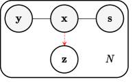
Figure 1: The graphical model that captures the modeling and Markov relations of the CPFSI method and also of the IBSI [11]. The solid arrows represent the generative assumptions, while the dotted red arrows represent the encoding relation between the input $\mathbf{x}$ and the representation $\mathbf{z}$.

CPFSI combines two conflicting goals: Invariant representation learning and representation learning for a downstream task. Specifically, we want to learn a representation $\mathbf{z}$ of the covariates $\mathbf{x}$, with the constraint that $\mathbf{z}$ contains as little information as possible about the sensitive attribute $\mathbf{s}$, i.e., we aim for $\mathbf{z}$ independent of $\mathbf{s}$ or $\mathbf{z}\bot\mathbf{s}$. While a faithful representation $\mathbf{z}$ innately contains much information about $\mathbf{x}$, we additionally ensure good performance on a selected downstream task by rewarding representations that contain sufficient information about $\mathbf{y}$. The covariates, target, and sensitive attribute are observable quantities, while $\mathbf{z}$ is obtained by encoding $\mathbf{x}$ (see Fig. 1). Thus, the training data contains realizations of $\mathbf{x}$, $\mathbf{y}$, and $\mathbf{s}$, which we use to learn our model.

III-A Lagrangian Formulation

We capture the three aims of CPFSI via information-theoretic quantities. Specifically, we measure the invariance of the representation $\mathbf{z}$ w.r.t. the sensitive attribute $\mathbf{s}$ via $I(\mathbf{s;z})$, its faithfulness regarding the covariates $\mathbf{x}$ via $I(\mathbf{x;z|s})$, and its utility for the downstream task via $I(\mathbf{y;z|s})$, respectively, where we condition on $\mathbf{s}$ to avoid conflict with the aim for invariance. With this, the Lagrangian formulation of the multi-objective optimization problem can be stated as follows:

Definition 1 (CPFSI)

In the setting of Fig. 1, the Conditional Privacy-Funnel with Side-Information (CPFSI) Lagrangian problem is

$$\min_{{p(\mathbf{z|x})}}\{\mathcal{L}_{CPFSI}:=I(\mathbf{s;z})-\gamma I(\mathbf{z;x|s})-\beta I(\mathbf{y;z|s})\}$$ (4)

for $\gamma,\beta\geq 0$.

Note that (4) differs from (3) by considering side information via the term $I(\mathbf{y;z|s})$. We thus recover the CPF of [5] by setting $\beta=0$. Using the Markov relations and the chain rule of mutual information, it is easy to show that $I(\mathbf{s;z})=I(\mathbf{z;x})-I(\mathbf{z;x|s})$. Hence, we can rewrite the above objective as

$$\mathcal{L}_{CPFSI}=I(\mathbf{z;x})-\alpha I(\mathbf{z;x|s})-\beta I(\mathbf{y;z|s})$$ (5)

with $\alpha=\gamma+1\geq 1$ and $\beta\geq 0$.

It is simple to relax the latter conditions and require only that $\alpha,\beta\geq 0$. We note that, given an appropriate choice of parameters, the CPFSI, CPF, and CFB are all equivalent to the following objective

$$\mathcal{L}_{FUNCK}:=\\ (1-\delta)I(\mathbf{z;x})+\delta I(\mathbf{s;z})-\gamma I(\mathbf{z;x|s})-\beta I(\mathbf{y;z|s}).$$ (6)

Setting $\delta=1$, we recover (4). For $\delta<1$, the first term antagonizes the reconstruction term $I(\mathbf{z;x|s})$, especially if $\gamma$ is small. Further, by setting $\alpha=0$ with $\beta>1$, (5) reduces to the CFB in (2). While, the case when $0\leq\beta\leq 1$ might have some relevance in applications with weak-supervision, e.g. noisy labels. Thus, (6) describes a family of training objectives that generalize the CPFSI, CFB and CPF and that allows to trade between their respective goals.

III-B Variational Bounds

Similar to [10], we can upper bound the mutual information between $\mathbf{x}$ and $\mathbf{z}$ using the non-negativity of the Kullback-Leibler divergence

$$I(\mathbf{z;x}) =\mathbb{E}_{p(\mathbf{x,z})}\log\frac{{p(\mathbf{z|x})}}{{p(\mathbf{z})}}$$

$$\leq\mathbb{E}_{p(\mathbf{x,z})}\log\frac{{p(\mathbf{z|x})}}{{q(\mathbf{z})}}$$

$$=\mathbb{E}_{p(\mathbf{x,y})}D_{KL}({p(\mathbf{z|x})}\|{q(\mathbf{z})})$$

where ${q(\mathbf{z})}$ is a variational approximation to the marginal distribution ${p(\mathbf{z})}=\mathbb{E}_{p(\mathbf{x})}{p(\mathbf{z|x})}$.

We are looking for lower bounding the remaining mutual information terms. Still using the non-negativity of the Kullback-Leibler divergence, we have

$$I(\mathbf{z;x|s}) =\mathbb{E}_{p(\mathbf{x,s,z})}\log\frac{{p(\mathbf{x|z,s})}}{{p(\mathbf{x|s})}}$$

$$\geq\mathbb{E}_{p(\mathbf{x,s,z})}\log\frac{{q(\mathbf{x|z,s})}}{{p(\mathbf{x|s})}}$$

$$=\mathbb{E}_{{p(\mathbf{x,s})}{p(\mathbf{z|x})}}\left[\log{q(\mathbf{x|z,s})}\right]+H(\mathbf{x|s})$$

where ${q(\mathbf{x|z,s})}$ is a variational approximation to the posterior ${p(\mathbf{x|z,s})}$. Likewise, we have

$$I(\mathbf{y;z|s})\geq\mathbb{E}_{p(\mathbf{s,y,z})}\left[\log{q(\mathbf{y|z,s})}\right]+H(\mathbf{y|s})$$

Analogously to the VAE [19, 20], we can adapt this model for scalable learning and inference. First, we drop from the optimization problem the terms that do not depend on the latent variable $\mathbf{z}$, such as $H(\mathbf{x|s})$ and $H(\mathbf{y|s})$. Second, we parameterize this stochastic model with deep neural networks with parameters $\theta$ and $\phi$ that will be optimized jointly. Specifically, the parameters $\theta$ belong to a stochastic encoder ${p_{\theta}({\mathbf{z|x}})}$, while the parameters $\phi$ belong to the variational approximations to the posteriors: The decoder ${q_{\phi}({\mathbf{x|z,s}})}$ and the predictive posterior ${q_{\phi}({\mathbf{y|z,s}})}$. The use of amortized inference of $\mathbf{z}$ allows exploiting the similarity between inputs to efficiently encode the underlying observations. In addition, we apply the reparameterization trick [19, 20] to $\mathbf{z}$, effectively allowing gradient backpropagation through the stochastic layers. The reparameterization trick consists of assuming that $\mathbf{z}$ can be decomposed into a stochastic part that does not depend on the model parameters, and a deterministic part that depends on the input $\mathbf{x}$. Assuming $\mathbf{z}\sim\mathcal{N}(\mu,\sigma\mathbf{I})$, we would have $z=\mu+\sigma\odot n$ with $\mathbf{n}\sim\mathcal{N}(\mathbf{0},\mathbf{I})$. Finally, we assume that ${p(\mathbf{x,y,s})}$ coincides with the empirical distribution of the dataset $\mathcal{D}$, which contains realizations $x$, $y$, and $s$, and we approximate the expectations over the representation $\mathbf{z}$ with Monte Carlo sampling, effectively replacing all the above expectations with averages.

Based on these considerations, we substitute the Lagrangian in (5) by the variational bound

$$\tilde{\mathcal{L}}_{CPFSI}:=\\ \frac{1}{S|\mathcal{D}|}\sum_{(x,y,s)\in\mathcal{D}}\sum_{z\sim{p_{\theta}({\mathbf{z}|x})}}D_{KL}({p_{\theta}({\mathbf{z}|x})}\|q(\mathbf{z}))\\ \quad-\alpha\log{q_{\phi}({x|z,s})}-\beta\log{q_{\phi}({y|z,s})}$$ (7)

where $|\mathcal{D}|$ is the dataset size and $S$ is the number of samples taken from the posterior ${p_{\theta}({\mathbf{z}|x})}$. The variational bound (7) is minimized over the network parameters $\theta$ and $\phi$.

In practice, we train our models with mini-batch gradient descent, adopt a deep latent Gaussian model with ${q(\mathbf{z})}$ following a standard multivariate normal with zero mean and identity covariance, and use a single sample $z$ from the posterior for training (i.e., $S=1$). The choices for the generative and predictive posteriors depend on the modeled dataset.

We note that our approximation to the objective conditions on the sensitive attribute $\mathbf{s}$ in the predictive posterior, unlike IBSI’s variational approximation in [12, Section 2.2]. This means that our model emphasizes the distinction between $\mathbf{z}$ and $\mathbf{s}$ in the predictor and has the extra feature of allowing interventions in the representation space, allowing for counterfactual predictions.

III-C Semi-supervised Learning

By extending the CPF objective to accept side-information $\mathbf{y}$, we introduced a way to learn latent structures about the input data guided by a supervision signal. This allows the CPFSI method to be adapted to semi-supervised learning or other forms of weak supervision. In this work, we adapted the objective to learn with a few labels with a simple strategy: We have set $\beta=0$ for observations without corresponding target label to obtain an extra loss term for the unsupervised observations. The unsupervised loss is then summed to the supervised loss scaled by $\max(|\mathcal{B}_{u}|/|\mathcal{B}_{s}|,1)$, where $|\mathcal{B}_{u}|$ and $|\mathcal{B}_{s}|$ are the unsupervised and supervised batch sizes, respectively. We note that a semi-supervised version of IBSI could have a similar strategy applied, since its variational approximation in [12] also includes a generative model.

IV Experimental Setup

In this section, we describe the experimental framework used in this study to characterize different instances of the FUNCK family of objectives and other models described above. Specifically, we describe the modeling choices, datasets, implementation and training details, and evaluation procedures.

IV-A Datasets

To provide a more thorough characterization of the underlying trade-offs and study the application of these methods on fairly common and realistic application scenarios, which are often characterized by relatively small amounts of tabular data. The experiments in this work were restricted to four tabular datasets with binary target $\mathbf{y}$ and binary attribute $\mathbf{s}$, namely the Adult, Dutch, Credit, and COMPAS datasets.

The target task in the Adult dataset is predicting if a person’s income larger than $50k. This dataset is one of the most commonly cited datasets in algorithmic fairness work and has 45k observations. The Dutch dataset predicts a binary attribute related with the person’s occupation. Both these datasets consist of census data and gender is the protected or sensitive attribute. The Credit dataset has 30k observations, we predict if the client will miss the payment in the following month, and gender is the sensitive attribute. Finally, the ProPublica COMPAS dataset, the target is recidivism within two years, while race is the sensitive attribute. This dataset has only approx. 6k observations.

We used one-hot encoding for the categorical features and standardized the numerical features for all datasets. Since the Dutch dataset did not contain numerical features, we created one based on target encoding of the age attribute in the training set followed by standard scaling. The numerical and categorical reconstruction losses were balanced using the numerical features’ variance, which are part of the Gaussian NLL loss.

All datasets were split as 18:2:5 for the training, validation, and test set, respectively. We further experimented with other, even smaller datasets (such as the German dataset with 1k observations), but were unable to lean useful representations from them.

IV-B Implementation and Training

Each model was trained on five different seeds. Each seed determines the model’s initial weights and selects a different split of a dataset, such that each replica is trained and evaluated on disjoint splits of the data. In total, we present the results of over 6000 trained models.

IV-B1 Models

We performed experiments on the variational approximations of IBSI [12] and different instances of the FUNCK family of objectives described in II and in Section III. These are the CPF [5], CFB [5], and CFPSI (Ours). For semi-supervised learning, we performed experiments on a semi-supervised version of the CPFSI and the Variational Fair Autoencoder (VFAE), proposed in [13]. All models were implemented with similar architectural choices. Both the encoder and decoder are feed-forward neural networks with ReLU activation functions, while the classifier is a logistic layer from the representation to the target attribute. Regarding IBSI, we did not follow the exact implementation from [12]. Instead, to enable a fair comparison between the objectives (and to avoid being confounded by effects due to their approximations), we implemented IBSI using similar approximations as our other models, essentially following [10].

IV-B2 Training

All models were trained for a maximum of 200 epochs using the Adam optimizer, learning rate of $0.001$, and batches of (at most) size 256. We reduced the learning rate when the validation loss demonstrated no improvements for at most 10 epochs. We also stopped training early after 20 epochs without improvements.

IV-B3 $\alpha,\beta$-tradeoff

All losses were weighted by two terms ($\alpha$ and $\beta$) that controlled the reconstruction and classification losses, respectively. The KL term was implicitly controlled by the total magnitude of both terms. These loss hyperparameters ranged from 1 to 1024 and were generated from the sequence $2^{2k},k=0,\ldots,5$. The CFB and CPF models had $\alpha$ and $\beta$ to zero, respectively. For IBSI (1), the $\alpha$ ranged between 0 and 1.

IV-B4 Semi-supervision

The level of supervision ranged from 4 to 256 labels per class in semi-supervised experiments. The reconstruction term weight was set to 1 to all semi-supervised experiments, while the weighting target cross-entropy term varied.

IV-C Evaluating Representations

One of the main goals of this work was to evaluate the learned encoders by way of their generated representations, $\mathbf{z}$. These were in turn evaluated in terms of classification error, different notions of invariance (a.k.a. ”fairness” or ”privacy”), and reconstruction error (fidelity or faithfulness to the input). All evaluated models were picked using the best validation loss, while all reported results are obtained from the test set’s representations.

Algorithm 1 describes broadly the evaluation procedure. Using a similar approach to [13], we trained a Logistic Regression (LR) and Random Forest (RF) to predict either the target or sensitive attribute from $z$. The latter was done to measure, linearly and non-linearly, the information content left by the encoders. In other words, these estimators were used as measurement instruments for the fairness and privacy of $z$. To control for overfitting on the test set, we repeated the evaluation five times on different splits of the test set and reported in the figures the median of these measurements. All RF predictors used 100 estimators.

Metrics The binary classifiers $f(\cdot)$ were evaluated in terms of accuracy, discrimination [14], and error-gap (See Supplementary Material for results). The reconstruction error of the numerical features was measured in terms of the mean-absolute error (MAE). Specifically, for a dataset $\mathcal{D}=\{(x_{i},y_{i},s_{i})\}_{i=1}^{N}$ the $i$-th observation has binary label $y_{i}$, binary sensitive attributes $s_{i}$, and representation $z_{i}$ of input $x_{i}$; let $N_{C}$ be the number of observation in the dataset when restricted to $C$. The discrimination or statistical parity gap measures independence between a binary classifier $f(\cdot)$ of $y_{i}$ and a sensitive attribute $s_{i}$.

$$\Delta_{disc}:=\left|\frac{\sum_{i:\,s_{i}=0}f(z_{i})}{N_{s=0}}-\frac{\sum_{i:\,s_{i}=1}f(z_{i})}{N_{s=1}}\right|$$

For the representation fidelity, i.e., for evaluating how well $x$ can be reconstructed from $z$, we used Linear and Random Forest regression. The evaluation of the representation’s fidelity to the input was restricted to a single numerical feature. The RF regressor was limited to a maximum depth of 8.

Since all our measurement were obtained from different partitions of each test dataset which were aggregated afterwards, the results’ variability for each model is explained by the different weight’s initialization, different training set splits, and the different configuration for the objectives in terms of $\alpha$ and $\beta$. Baseline values were calculated by adapting the evaluation above to the original dataset without $s$ as a covariate.

Algorithm 1 Representation Evaluation.

  $t\in\{x_{j},y,s\}$;   $z\leftarrow\textsc{Encoder}_{\theta}(x)$;   $metrics\leftarrow\textsc{List}()$

  for $(z_{tr},t_{tr}),(z_{te},t_{te})$ in $\textsc{KFold}(z,t,k=5)$ do

      for Estimator in $[\textsc{LR},\textsc{RF}]$ do

        Estimator.fit$(z_{tr},t_{tr})$

        $metrics\ \texttt{++}\ \textsc{Evaluator}(\textsc{Estimator},z_{te},t_{te}[,s_{te}])$

  return $metrics$

IV-D Fair Classification using the Predictive Posterior

In addition to evaluating the fairness of the latent representation, we also evaluate the learned predictive posterior or binary classifier of the fully and semi-supervised models. To this end, we examined a form of fair classification where we intervene at test time in the observed $\mathbf{s}$. We used this to study the effect on discrimination of counterfactual predictions. However, we do not seek to predict the effect of actual interventions, but only make obtain fairer predictions on observational data without making any assumption about the causal mechanisms to generate the data. Specifically, we explored two straightforwards interventions on $s$: flipping the binary value of $s$, and fixing $s$ to $0.5$. This approach is described in Algorithm 2.

Algorithm 2 Predictive Posterior Evaluation.

  $z\leftarrow\textsc{Encoder}_{\theta}(x)$;  $metrics\leftarrow\textsc{List}()$

  for s’ in $[s,1-s,1/2]$ do

      $metrics\ \texttt{++}\ \textsc{Evaluator}(\textsc{Posterior}_{\phi},z[,s^{\prime}])$

  return $metrics$

V Results

Following the evaluation described above (Section IV-C), we highlight our key findings in the fully and semi-supervised settings. Furthermore, the results are subdivided between the representations’ evaluation in terms of fairness (Section V-A1) and privacy (Section V-A2), and an evaluation of the models’ capabilities for fair classification (See Section V-A3).

In the supplementary material, we provide extra figures for all datasets, different latent-sizes, and replace the fairness evaluation with the error-gap metric.

V-A Full Supervision

V-A1 Representation Fairness

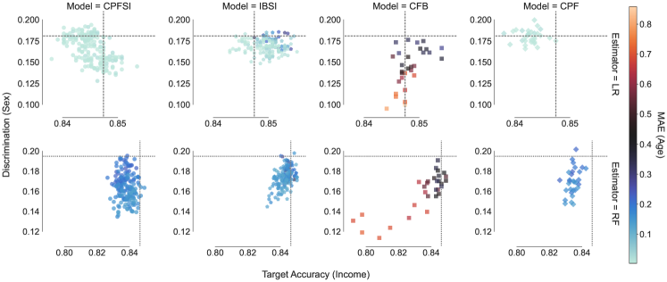
Figure 2: Representation’s fairness for $|\mathbf{z}|=32$ on the Adult dataset. The dashed line marks the estimators – Logistic Regression (top) and Random Forest (bottom) – evaluated on the original dataset. The color scale represents the mean absolute reconstruction error from Linear Regression and Random Forest Regressor of one of a numerical feature of $x$ from $z$.

In Fig. 2, we evaluated different $\alpha$ and $\beta$ configurations to characterize the compromise between discrimination, fidelity, and accuracy in the representations generated from the test set of the Adult dataset. Most methods, including the CPFSI, had configurations that encoded the input data such that it matched or exceeded the baselines accuracies with lower discrimination, which demonstrates the applicability of these techniques in unbiasing data.

A key point to be made is that CFB achieves the lowest discrimination in most datasets. However, this is done at the expense of losing most information about the input, since CFB learns exclusively task-specific representations. In contrast, the CPFSI has both high accuracy and low discrimination while encoding the input data with high fidelity. Hence, the CPFSI learns task-agnostic representations that can be useful in application settings where there are multiple or unknown downstream tasks.

Regarding IBSI’s representations, these can be the most predictive of the target attribute. Nevertheless, this doesn’t occur without penalizing the discrimination more than the CPFSI. This observation is most obvious in the Dutch dataset (see supplementary material). Thus, in comparison to IBSI, CPFSI enables fairer downstream classification from representations faithful to the input and the target. This can be verified both in the linear (LR) and nonlinear (RF) evaluations of the representations.

The remaining results for the Dutch, Credit, and Compas dataset can be found in the supplementary material. Generally, these results were clearer for larger datasets. Similarly to [12], it is harder to differentiate between methods for small datasets, which suggests a clear limitation of these techniques in situations where data collection is too expensive or cumbersome.

V-A2 Representation Privacy

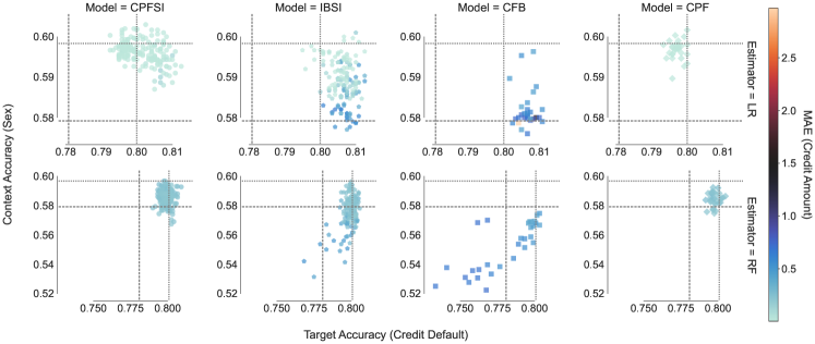
Figure 3: Representation’s privacy for $|\mathbf{z}|=32$ on the Credit dataset. The dashed lines correspond to the baseline of majority classifier, while the dotted lines correspond to the baseline of the row estimator – Logistic Regression (top) and Random Forest (bottom) – on the original dataset. The color scale represents the Linear Regression and Random Forest Regressor reconstruction error of one of the numerical features of $x$ from $z$.

In Fig. 3, we describe the compromise between the accuracies on the target and ”sensitive” attributes on the Credit dataset. All models show that information leakage (i.e., high accuracy on the sensitive attribute) is positively correlated with discrimination. Despite the original intent of privacy-preservation – more precisely privacy-awareness – of objectives like the CPF, the results illustrate that it was actually the methods targeting fair classification that had consistently the lowest predictiveness (leakage) of the sensitive (private) attribute. This result is actually not surprising, and any confusion stems only from the nomenclature of these methods. Since the privacy funnels favors task-agnostic representations where $\mathbf{z}$ carries more information about $\mathbf{x}$, it occurs that the funnel objectives will leak more information about $\mathbf{s}$. Whereas, the information bottleneck objectives favor compressing the information about $\mathbf{x}$ and learn task-specific representations for just $\mathbf{y}$. Likewise, if $\mathbf{y}$ is predictive to $\mathbf{s}$, then, fair classification is only possible if we lose some accuracy. However, this should affect learning to a lesser extent than $\mathbf{x}$ predicting $\mathbf{s}$, since typically $\mathbf{x}$ are high-dimensional feature vectors and more predictive of $\mathbf{s}$ than $\mathbf{y}$. In all cases, however, there is an inherent trade-off between privacy, reconstruction fidelity, and accuracy, that depends on the relation between variables.

Regarding IBSI, we see a conflict between the task-specific objective and the obtained results. On the one hand, the variational bound in [12] forces these models to have a decoder, which encourages learning task-agnostic representations with high fidelity to the input. On the other hand, the range for the Lagrange multipliers in IBSI forces the compressive term – the KL-divergence term – to have a strictly larger weighting than the reconstruction term – the decoder’s cross-entropy. In summary, the approximation and implementation create a discrepancy between the true objective and actual properties of the encoder. However, similar to CPFSI, IBSI generates representations both with high-fidelity and low information leakage.

In the supplementary material, we show how the size of the latent space can influence the information leakage of $\mathbf{s}$. Specifically, we believe that the dimensionality of the latent space affects our models in two ways. First, since we conditioned by simply concatenating $s$ in $z$, the dimensionality of $\mathbf{z}$ controls the relative strength of the conditioning. Second, the dimensionality defines a potential bottleneck in the architecture that directly affects the trade-off between reconstruction fidelity and leakage, and that thus has to be taken into account jointly with the parameters $\alpha$ and $\beta$ of CPFSI (e.g., small latent dimensions enforce stronger compression, reducing leakage and reconstruction fidelity). In other words, we show that if the latent space is too large, then we risk increasing the information leakage about $\mathbf{s}$ while not improving the accuracy considerably.

V-A3 Fair Classification using the Predictive Posterior

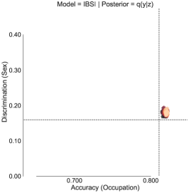
(a)

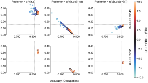
(b)

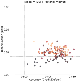
(c)

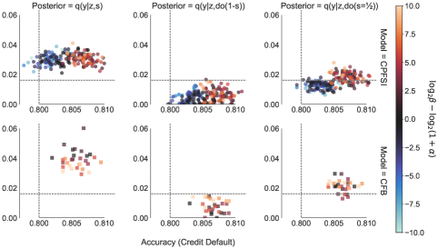
(d)

Figure 4: Comparison between predictive posteriors on the Dutch (top) and Credit (bottom) datasets for different interventions on the sensitive attribute $\mathbf{s}$.

In this set of experiments we perform classification using the learned predictive posterior ${q_{\phi}({\mathbf{y|z,s}})}$ and intervene in the representation space by fixing $\mathbf{s}$ according to two predefined rules (Section 2). Further, one of the interventions on the sensitive attribute also removes the requirement of having the sensitive attribute at test time.

This suggests an alternative approach to fair classification that is new to the best of our knowledge. It consists of finding an invariant representation regarding the protected attributes and a policy to intervene in $\mathbf{s}$ that achieves the most fairness and retains predictive performance. This approach is possible for any conditional predictive posteriors and/or classifiers like the CPFSI, CFB, and the semi-supervised version of the VFAE.

In Fig. 4 we show that intervening on a conditional classification can be useful to obtain fairer outcomes while preserving accuracy. We compare against the variational formulation of IBSI [12], which does not allow this manipulation. In addition, we show that for fair classification in the fully-supervised case, a conditional classifier like the CFB is sufficient and there is no need for CPFSI’s decoder. Our results indicate that the best intervention strategy depends on the dataset, but so far, we could not conclusively trace this dependency to the relation between $\mathbf{y}$ and $\mathbf{s}$. In any case, providing $s=1/2$ to the predictive posterior appears to consistently decrease discrimination while maintaining accuracy, compared to providing the true sensitive label.

V-B Semi-supervision

V-B1 Representation Invariance

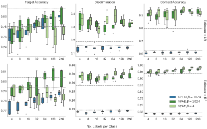
Figure 5: Number of labels’ influence on the representation quality for $\alpha=1$ for each model on the Dutch dataset. The dashed and dotted lines mark the unsupervised (CPF) and fully-supervised baselines, respectively.

This set of results in the semi-supervised setting showcases the potential of CPFSI for invariant representation learning with just a few labels per class. In Fig. 5 on the Dutch dataset, a few labels allow improving target accuracy while preserving the invariance constraint compared to the unsupervised case. In conclusion, a small amount of label helps to find more meaningful invariant representations. In comparison with the semi-supervised version of the VFAE (without the Maximum-Mean Discrepancy (MMD) term enforcing invariance), we see that CPFSI achieves comparable predictive accuracy while maintaining a lower discrimination and information leakage about the sensitive attribute. Furthermore, CPFSI is simpler to implement and train than the hierarchical (semi-supervised) VFAE. Regarding the remaining datasets, we observe that both discrimination and target accuracy results are comparable, but the information leakage is substantially higher for the VFAE.

We conjecture that reason the main reason VFAE achieves higher leakages comes from modeling the variational posterior ${q(\mathbf{z_{1}|x,s})}$. In dealing with this issue, the authors introduced a MMD term in the objective to encourage an invariant marginal posterior ${p(\mathbf{z_{1}|s})}$. We did not observe an added benefit in adding a MMD penalty to the CPFSI Lagrangian. Also, we do not encounter a practical benefit on the added complexity of the VFAE’s hierarchical model.

V-B2 Fair Classification using the Predictive Posterior

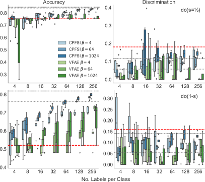
Figure 6: Number of labels’ influence on the predictive posterior quality for $\alpha=1$ and different $\beta$ on the Adult (top) and Dutch (bottom) dataset. The dashed (red) line marks the majority classifier and the Logistic Regression’s discrimination on the original dataset with full-supervision. The dotted and dash-dotted lines mark the fully-supervised results for the interventions $\mathrm{do}(1\!-\!s)$ and $\mathrm{do}(s\!=\!\nicefrac{{1}}{{2}})$, respectively.

Figure 6 illustrates how with just a few labels per class, it is possible to learn a fair classifier with CPFSI. For the Adult dataset (top row) we see that the VFAE can not learn a useful classifier for different $\beta$. Other experiments also verified this without intervening in $s$. Conversely, CPFSI converges to fully-supervised performance with increasing the number of labels per class. For the Dutch dataset (bottom row) the VFAE exhibits lower discrimination at the expense of lower accuracy, in comparison to CPFSI that achieves superior predictive performance overall. For each dataset, we used the best $s$ intervention according to Section V-A3. Further results can be found in the supplementary material.

VI Discussion

Information-theoretic objectives are a concise way to conveniently specify multiple requirements from first principles. In this work, we focused on deep invariant representation learning and characterized the FUNCK family of objectives with desiderata in fairness, privacy, predictive performance, and faithfulness to the input data.

Our results revealed a substantial information leakage by the encoded inputs. This is exacerbated by the fact that there is no privacy guarantee for each individual, given that any observation is at risk of revealing some private information. As mentioned above, the term privacy was used loosely, and we are simply reusing the terminology from previous work.

High representation fidelity is an indication of the usefulness of the representation in undefined downstream tasks, and this is achieved by CPF, CPFSI, and IBSI. While IBSI is targeted at a single task, by applying the chain rule for mutual information to IBSI, the authors of [12] introduced an artifact in the resulting variational bound that encourages high-fidelity representations. In contrast, CFB, which is also specialized to a single task, has representations with high reconstruction error that can be considered useless for an arbitrary downstream task. Nevertheless, the simplicity of the CFB allows for better encoding in terms of fairness and information leakage. We have identified CPFSI as covering the middle ground between these extremes, allowing to trade smoothly between fairness, privacy, predictive performance, and reconstruction fidelity. Further, while we focused on the semi-supervised case, CPFSI can easily be extended towards other weak supervised scenarios or settings where we aim to learn a shared representation that is invariant to some context $\mathbf{s}$. Much like [13], we could also extend our work to the domain adaptation setting. Given the relation of the variational bound with previous work, our method could also provide a weakly supervised alternative to the CFB method. Finally, since our variational decoder depends on the sensitive attribute, CPFSI, CPF, and IBSI are capable of controllable data generation. It was out of the scope of this work to investigate this.

Selecting the desired trade-off between fairness, privacy, predictive performance, and reconstruction fidelity requires setting $\alpha$ and $\beta$. This non-trivial task depends on the user preferences and could the subject of techniques like Bayesian optimization or other approaches to multi-objective optimization.

All models were restricted to a particular approximation and architectural choices in the framework of amortized variational inference parameterized by neural networks. As such, considerations about the objectives must be interpreted carefully, since it is not obvious to what extent statements based on the objective can carry over to the variational bound derived from its Lagrangian. In particular, situations where the sensitive attribute $\mathbf{s}$ and the target $\mathbf{y}$ are correlated, could yield random or degenerate representations regarding $\mathbf{y}$ when training an unsupervised model since removing the influence of $\mathbf{s}$ can also remove all the relevant information in $\mathbf{z}$. While we believe that our approximations to the Lagrangian objectives are flexible enough to be accurate, studying the effect of any these choices is out-of-the scope of this study.

We finally briefly investigate the effect of conditioning on the sensitive attribute $\mathbf{s}$ on predicting the target $\mathbf{y}$. This sets apart our CPFSI, CPF, and CFB [5] from IBSI [12]. On the one hand, since any information in $\mathbf{s}$ that is useful for reconstructing $\mathbf{x}$ or classifying $\mathbf{y}$ is given unaltered to the decoder and predictive posterior, there is no longer the necessity for $\mathbf{z}$ to learn unnecessary information about $\mathbf{s}$ from the input, i.e., conditioning on $\mathbf{s}$ enables a representation $\mathbf{z}$ that is invariant w.r.t. $\mathbf{s}$. On the other hand, a representation $\mathbf{z}$ that is obtained by feeding $\mathbf{s}$ to both variational decoder and predictive posterior may not suffice to achieve satisfactory reconstruction or classification accuracy if the actual decoder and classifier are not provided with the sensitive attribute. Thus, apparently, the trade-off between fairness/invariance, on the one hand , and performance on a downstream task on the other hand appears to be directly affected by whether the variational distributions are conditioned on the sensitive attribute.

To make this intuition precise, we now theoretically investigate the case where we are only interested in classification, i.e., a setting similar to the CFB. Specifically, we compare the following two optimization problems:

$$\min_{\begin{subarray}{c}p(\mathbf{z}|\mathbf{x})\in\mathcal{E}\\ q(\mathbf{y}|\mathbf{z},\mathbf{s})\in\mathcal{C}\end{subarray}}\quad I(\mathbf{z};\mathbf{s})\quad\text{s.t. }\mathbb{E}_{p(\mathbf{s,y,z})}\left[-\log{q(\mathbf{y|z,s})}\right]\leq\varepsilon$$ (8a)

and

$$\min_{\begin{subarray}{c}p(\mathbf{z}|\mathbf{x})\in\mathcal{E}\\ q(\mathbf{y}|\mathbf{z})\in\mathcal{C}\end{subarray}}\quad I(\mathbf{z};\mathbf{s})\quad\text{s.t. }\mathbb{E}_{p(\mathbf{y,z})}\left[-\log{q(\mathbf{y|z})}\right]\leq\varepsilon.$$ (8b)

For the sake of argument, we give the neural network implementing the classifier sufficient expressive power such that it can learn the true posterior, i.e., ${p(\mathbf{y|z,s})},\,{p(\mathbf{y|z})}\in\mathcal{C}$. With this, the above optimization problems simplify to

$$\min_{p(\mathbf{z}|\mathbf{x})\in\mathcal{E}}\quad I(\mathbf{z};\mathbf{s})\quad\text{s.t. }H(\mathbf{y}|\mathbf{z},\mathbf{s})\leq\varepsilon$$ (9a)

and

$$\min_{p(\mathbf{z}|\mathbf{x})\in\mathcal{E}}\quad I(\mathbf{z};\mathbf{s})\quad\text{s.t. }H(\mathbf{y}|\mathbf{z})\leq\varepsilon.$$ (9b)

This is similar to stopping training as soon as the classification error of the predictive posterior on the validation set falls below a threshold.

Since by the fact that $H(\mathbf{y}|\mathbf{z},\mathbf{s})\leq H(\mathbf{y}|\mathbf{z})$ (conditioning reduces entropy), the feasible set $\mathcal{E}$ for the former optimization problem in (9a) is a superset of the feasible set $\mathcal{E}$ of (9b). Hence, conditioning the predictive posterior on the sensitive attribute $\mathbf{s}$ achieves at least as small $I(\mathbf{s};\mathbf{z})$ as not conditioning. At the same time, while $H(\mathbf{y}|\mathbf{z},\mathbf{s})\leq\varepsilon$ does not imply that $H(\mathbf{y}|\mathbf{z})\leq\varepsilon$. Thus, the error probability of a classifier that relies on $\mathbf{z}$ alone and that is not provided with the sensitive attribute $\mathbf{s}$ may be larger for $\mathbf{z}$ obtained from solving (9a) than for $\mathbf{z}$ obtained from solving (9b).

The last statement needs to be qualified: There is no one-to-one correspondence between conditional entropy and error probability, there are only bounds (e.g., [23, 24]). However, we believe that aside from the theoretical argument provided via conditional entropy, the last statement is also plausible from a learning perspective: Optimizing (9b) ensures that $\mathbf{z}$ is useful for classification on its own, at least for a classifier with the same architecture as the variational classifier ${q(\mathbf{y|z})}$. In contrast, the $\mathbf{z}$ obtained by solving (9a) is not necessarily useful on its own, not even for a classifier with the same expressive power as the variational classifier ${q(\mathbf{y|z,s})}$. Information about $\mathbf{y}$ contained in $\mathbf{z}$ may be accessible only with side information $\mathbf{s}$, but not individually. Future work shall study the interplay between conditioning in the predictive posterior(s) and the characteristics of the learned representations in more detail.

VII Conclusion

In an era where data collection is ubiquitous, learning representations that remain both useful and invariant to a nuisance factors of variations still remains a key challenge, specially when learning with almost no supervision. Therefore, we extended the analysis of the VFAE, IBSI, CPF, CFB, and proposed the CPFSI: A new method for invariant representation learning in the semi-supervised setting, which generalizes the recently proposed CPF.

In this regard, the CPFSI demonstrated substantial benefits in learning invariant representations with few labels. We empirically show that with a few labels, it is possible to learn fairer representations and reduce information leakage. Moreover, the CPFSI is also capable of fair classification and achieves lower discrimination than non-conditional models when we intervene on the sensitive attribute. This structural property of our model is one of the main differences between this work and [12]. However, it was also shown that these information-theoretic objectives require careful use in applications that require invariant representations, as private data sharing. It was further demonstrated that the CFB (essentially a conditional version of IBSI) provides a better alternative to the IBSI, if one does not need faithful representation of the input.

While small and tabular datasets are often encountered in industry applications [25], DNNs are most limited when applied to domains with small and tabular dataset [26]. Nonetheless, research in FAccT has seen an increasing number of work that applies DNNs to these domains. While we demonstrated that CPFSI is competitive with previous work across tabular datasets, we also showed many of the limitations of these methods in run-of-the-mill applications like the ones illustrated by the tabular datasets we studied.

Appendix A Full Supervision (All Datasets)

A-A Representations Fairness

In the figures below, the evaluated representations have 32 dimension and the color scale represents the reconstruction error of one numerical feature. The representations were evaluated with linear (LR) and nonlinear (RF) predictors. in adult,dutch,credit,compas

Figure 7: Trade-off between representation fairness, accuracy, and fidelity on the dataset.

A-B Representations Privacy

In the following figures, the evaluated representations have 32 dimension and the color scale represents the reconstruction error of one numerical feature. The representations were evaluated with linear (LR) and nonlinear (RF) predictors. in adult,dutch,credit,compas

Figure 8: Trade-off between representation privacy, accuracy, and fidelity on the dataset.

A-C Fair Classification using the Predictive Posterior

In this set of figures, the LR and RF are linear and nonlinear predictors, respectively. in adult,dutch,credit,compas

(a)

(b)

Figure 9: Fair classification results. Comparison between predictive posteriors for different interventions on $s$ on the dataset.

Appendix B Semi-Supervision (All Datasets)

B-A Representation Fairness & Privacy

In the following figures, the dotted line is the CPFSI’s representation baseline with full supervision. The dashed line is the baseline on the original dataset. All models were trained with $\alpha=1$ and the estimators LR and RF are linear and nonlinear predictors, respectively. in adult,dutch,credit,compas

Figure 10: Semi-supervised results on the dataset.

B-B Fair Classification using the Predictive Posterior

In the figures below, the dashed (red) line marks the majority classifier and the Logistic Regression’s discrimination on the original dataset with full-supervision. The dotted and dash-dotted lines mark the fully-supervised results for the interventions $\mathrm{do}(1\!-\!s)$ and $\mathrm{do}(s\!=\!\nicefrac{{1}}{{2}})$, respectively. All figures in this section show results with $\alpha=1$ and $\beta=1024$. in adult,dutch

Figure 11: Fair classification results on the dataset.

in credit,compas

Figure 12: Fair classification results on the dataset.

Appendix C Latent Space Size

C-A Representations Fairness

In the next figures, the representation were evaluated with linear models and the color scale represents the representation fidelity. in adult,dutch,credit,compas

Figure 13: Trade-off between representation’s fairness, accuracy, size on the dataset.

C-B Representations Privacy

In this section’s figures, the representation were evaluated with linear models and the color scale represents the representation fidelity. in adult,dutch,credit,compas

Figure 14: Trade-off between representation’s privacy, accuracy, and size on the dataset.

C-C Representation Fairness vs. Privacy

In this section, representations were evaluated with linear models (Linear and Logistic Regression) and the color scale represents the target-accuracy. in adult,dutch,credit,compas

Figure 15: Trade-off between error-gap (fairness), context-accuracy (privacy), and target-accuracy on the dataset.

Appendix D Error Gap

The error gap of a binary classifier measures accuracy parity between two subgroups is defined as

$$\Delta_{err}:=\left|\frac{\sum_{i:s_{i}=0}\mathbb{I}(f(z_{i})\neq y_{i})}{N_{s=0}}-\frac{\sum_{i:s_{i}=1}\mathbb{I}(f(z_{i})\neq y_{i})}{N_{s=1}}\right|$$

In the figures below, the color scale represents the target-accuracy and the representations were evaluated with linear estimators. in adult,dutch,credit,compas

Figure 16: Trade-off between error-gap (fairness), context-accuracy (privacy), and target-accuracy on the dataset.

References

- [1] N. Mehrabi, F. Morstatter, N. Saxena, K. Lerman, and A. Galstyan, “A survey on bias and fairness in machine learning,” ACM Comput. Surv., vol. 54, no. 6, Jul. 2021.
- [2] X. Huang, D. Kroening, W. Ruan, J. Sharp, Y. Sun, E. Thamo, M. Wu, and X. Yi, “A survey of safety and trustworthiness of deep neural networks: Verification, testing, adversarial attack and defence, and interpretability,” Computer Science Review, vol. 37, p. 100270, 2020.
- [3] C. Dwork, F. McSherry, K. Nissim, and A. Smith, “Calibrating noise to sensitivity in private data analysis,” in Proc. Third Conf. on Theory of Cryptography (TCC). Berlin, Heidelberg: Springer-Verlag, 2006, p. 265–284.
- [4] A. Makhdoumi, S. Salamatian, N. Fawaz, and M. Médard, “From the information bottleneck to the privacy funnel,” in Proc. IEEE Information Theory Workshop (ITW). IEEE, 2014, pp. 501–505.
- [5] B. Rodríguez-Gálvez, R. Thobaben, and M. Skoglund, “A variational approach to privacy and fairness,” in Proc. IEEE Information Theory Workshop (ITW). IEEE, 2021, pp. 1–6.
- [6] F. Locatello, S. Bauer, M. Lucic, G. Raetsch, S. Gelly, B. Schölkopf, and O. Bachem, “Challenging common assumptions in the unsupervised learning of disentangled representations,” in Proc. Int. Conf. on Machine Learning (ICML), 2019, pp. 4114–4124.
- [7] F. Locatello, M. Tschannen, S. Bauer, G. Rätsch, B. Schölkopf, and O. Bachem, “Disentangling factors of variations using few labels,” in International Conference on Learning Representations, 2020.
- [8] B. C. Geiger and I. S. Fischer, “A comparison of variational bounds for the information bottleneck functional,” Entropy, vol. 22, no. 11, 2020.
- [9] N. Tishby, F. Pereira, and W. Bialek, “The information bottleneck method,” Proc. Allerton Conf. on Communication, Control and Computation, vol. 49, 07 2001.
- [10] A. A. Alemi, I. Fischer, J. V. Dillon, and K. Murphy, “Deep variational information bottleneck,” in Proc. Int. Conf. on Learning Representations (ICLR), 2017.
- [11] G. Chechik and N. Tishby, “Extracting relevant structures with side information,” Advances in Neural Information Processing Systems, vol. 15, 2002.
- [12] D. Moyer, S. Gao, R. Brekelmans, A. Galstyan, and G. Ver Steeg, “Invariant representations without adversarial training,” in Advances in Neural Information Processing Systems, vol. 31, 2018.
- [13] C. Louizos, K. Swersky, Y. Li, M. Welling, and R. Zemel, “The variational fair autoencoder,” 2015.
- [14] R. Zemel, Y. Wu, K. Swersky, T. Pitassi, and C. Dwork, “Learning fair representations,” in Proc. Int. Conf. on Machine Learning (ICML), 2013, p. III–325–III–333.
- [15] H. Edwards and A. Storkey, “Censoring representations with an adversary,” in Proc. Int. Conf. on Learning Representations (ICLR), 2016, pp. 1–14.
- [16] B. Razeghi, F. P. Calmon, D. Gündüz, and S. Voloshynovskiy, “Bottlenecks CLUB: Unifying information-theoretic trade-offs among complexity, leakage, and utility,” 2022.
- [17] E. Creager, D. Madras, J.-H. Jacobsen, M. Weis, K. Swersky, T. Pitassi, and R. Zemel, “Flexibly fair representation learning by disentanglement,” in Proc. Int. Conf. on Machine Learning (ICML), 2019, pp. 1436–1445.
- [18] J. Song, P. Kalluri, A. Grover, S. Zhao, and S. Ermon, “Learning controllable fair representations,” in Proc. Int. Conf. on Artificial Intelligence and Statistics (AISTATS), 2019, pp. 2164–2173.
- [19] D. P. Kingma and M. Welling, “Auto-encoding variational Bayes,” in Proc. Int. Conf. on Learning Representations (ICLR), Banff, AB, Canada, Apr. 2014.
- [20] D. J. Rezende, S. Mohamed, and D. Wierstra, “Stochastic backpropagation and approximate inference in deep generative models,” in Proc. Int. Conf. on Machine Learning (ICML), vol. 32, 2014, pp. 1278–1286.
- [21] N. Tishby and N. Zaslavsky, “Deep learning and the information bottleneck principle,” in Proc. IEEE Information Theory Workshop (ITW), 2015, pp. 1–5.
- [22] A. M. Saxe, Y. Bansal, J. Dapello, M. Advani, A. Kolchinsky, B. D. Tracey, and D. D. Cox, “On the information bottleneck theory of deep learning,” in Proc. Int. Conf. on Learning Representations (ICLR), 2018.
- [23] T. S. Han and S. Verdu, “Generalizing the Fano inequality,” IEEE Transactions on Information Theory, vol. 40, no. 4, pp. 1247–1251, 1994.
- [24] M. Feder and N. Merhav, “Relations between entropy and error probability,” IEEE Transactions on Information Theory, vol. 40, no. 1, pp. 259–266, 1994.
- [25] D. Dua and C. Graff, “UCI machine learning repository,” 2017.
- [26] L. Grinsztajn, E. Oyallon, and G. Varoquaux, “Why do tree-based models still outperform deep learning on typical tabular data?” in Thirty-sixth Conference on Neural Information Processing Systems Datasets and Benchmarks Track, 2022.