The long-term spectral changes of eta Carinae: are they caused by a dissipating occulter as indicated by cmfgen models?

Abstract

Eta Carinae ($\eta$ Car) exhibits a unique set of P Cygni profiles with both broad and narrow components. Over many decades, the spectrum has changed – there has been an increase in observed continuum fluxes and a decrease in Fe ii and H i emission line equivalent widths. The spectrum is evolving towards that of a P Cygni star such as P Cygni itself and HDE 316285. The spectral evolution has been attributed to intrinsic variations such as a decrease in the mass-loss rate of the primary star or differential evolution in a latitudinal-dependent stellar wind. However intrinsic wind changes conflict with three observational results: the steady long-term bolometric luminosity; the repeating X-ray light curve over the binary period; and the constancy of the dust-scattered spectrum from the Homunculus. We extend previous work that showed a secular strengthening of P Cygni absorptions by adding more orbital cycles to overcome temporary instabilities and by examining more atomic transitions. cmfgen modeling of the primary wind shows that a time-decreasing mass-loss rate is not the best explanation for the observations. However, models with a ‘small’ dissipating absorber in our line-of-site can explain both the increase in brightness and changes in the emission and P Cygni absorption profiles. If the spectral evolution is caused by the dissipating circumstellar medium, and not by intrinsic changes in the binary, the dynamical timescale to recover from the Great Eruption is much less than a century, different from previous suggestions.

1 Introduction

The $\eta$ Car spectrum recorded in the 1980s was very unusual for an LBV (or P Cygni) star (Hillier et al., 2001a; Humphreys & Davidson, 1994). It exhibited broad wind lines (FWHM$\sim 800$ km s^-1) of H i, Fe ii, and He i  which are now understood to be associated with the primary stellar wind, although He i is also likely to be influenced by the wind-wind collision (WWC) zone and the radiation of the secondary star. Very prominent narrow emission lines (FWHM$\sim$ 20–80 km s^-1) of H i, He i, Fe ii and [Fe ii], superimposed on the spectrum, arise in the Weigelt clumps (Davidson et al., 1995). Both the Fe ii and [Fe ii] lines exhibited a broad base with similar FWHM values to that of the primary wind lines. The broad [Fe ii] lines are unusual and are not seen in other stars with strong stellar winds at similar excitation regimes (e.g. HDE 316285, Hillier et al., 2001a). They are now understood to originate in the stellar wind, but their strength relative to the stellar continuum has been enhanced by the occulter (Hillier et al., 2001b). The same effect makes the narrow components unexpectedly prominent.

Mehner et al. (2019), using the dusty Homunculus as a calorimeter in the infrared, demonstrated that the binary luminosity has been reasonably constant over the period 1968 to 2018 with possible variations associated with the 5.53-year binary orbit. Yet from 2000 to 2020 the stellar brightness increased by more than a decade in the UV (Gull et al., 2021). The dust in the Homunculus absorbs the bulk of the radiation from the visible into the FUV with subsequent re-emission in the infrared. The pronounced stability of the X-ray light curve over the past five binary cycles (Espinoza Galeas et al., 2021; Corcoran et al., 2017) confirms that the stellar winds and their collision have been stable over the past two decades.

Mehner et al. (2012) reported that the stellar continuum at 3950Å reflected by Weigelt clump D stayed constant over two cycles (1999 to 2010) while the flux of the central star increased more than ten-fold (their Fig. 12).

Damineli et al. (2019) suggested that a dissipating dusty structure that partially occulted the central star and the extended winds would explain the reports by Gull et al. (2009) and by Mehner et al. (2014) that while the central star brightened in the visible and UV, the Weigelt clumps (Weigelt & Ebersberger, 1986) remained at constant flux, leading to an effective decrease in line equivalent widths since the EW is the line flux divided by the continuum inside the slit.

Long-term strength decreases of some broad emission lines have been reported based on both ground-based and STIS observations made by Mehner et al. (2010, 2011, 2012, 2015, 2019); Martin et al. (2021); Davidson et al. (2018). Those authors suggested that the strength decrease might be due to the intrinsic evolution of the central star and that the secular brightness increase could be produced by a decrease in $\eta$ Car’s primary wind density or a decrease in circumstellar extinction. Another suggestion was that the latitude-dependent wind evolves differently in the equator and polar regions (Mehner et al., 2015). A latitude-dependent stellar wind was previously proposed by Smith et al. (2003b), who invoked rotation of the star as the cause. Groh et al. (2012a) showed that these observations are more likely explained by the ionization impact of the hot secondary modifying the primary wind structure. Moreover, the fast-rotator LBVs show S-Doradus instabilities, not seen in slow rotators and not present in $\eta$ Car, suggesting that $\eta$ Car might be a slow rotator, although this is not what is expected in a binary star merger.

The trend in the system’s photometric brightness (Damineli et al., 2019) along with a study of direct versus reflected line emission (Damineli et al., 2021, see also Mehner et al. 2015) – suggested that the long-term weakening of the emission lines could be better explained by a drop in circumstellar extinction along our line-of-sight (LOS) without recourse to intrinsic changes in $\eta$ Car A.

The impact of the dissipating occulter on spectral features is complicated, since both the line and continuum forming regions in $\eta$ Car are extended, and since different spectral lines are formed at different locations in the stellar wind. Thus, we first present a qualitative summary of the impact of an occulter on the intrinsice spectrum, which is complemented by the semi-quantitative cmfgen model described in Sect. 4.

Fig. 1 shows a schematic view of the five main regions contributing to the observed spectrum of $\eta$ Car. Taking advantage of STIS/HST observations makes it possible to disentangle the spectrum of the Weigelt clumps (region C) with their nebular emission lines and reflected continuum (which are relatively small in amplitude) from the central sources. Typical seeing from the ground of 1 to 2 arcsec (2300 to 4600 au) while HST/STIS spatial resolution is 0$\farcs$1 (230 au). The spectrum reflected from the Homunculus (region D) can also be resolved (for example, at the FOS 4 position) even from ground-based observations (Davidson & Humphreys, 1997). The central region is unresolved and is composed of $a)$ the central star plus its inner wind (region A) – the major source of light in the system, the source of both the stellar continuum and the very broad P Cygni spectral features profiles; and $b)$ the outer wind (region B) which contributes with relatively broad lines and some continuum flux. The occulter (region E) partially blocks the wind region but not the Weigelt clumps.

The occulter apparently blocks the central stellar core and part of the extended primary wind. As it dissipates, the contribution from the primary wind increases by a factor $\sim$2 while the core (continuum) increased $\sim$10-fold.

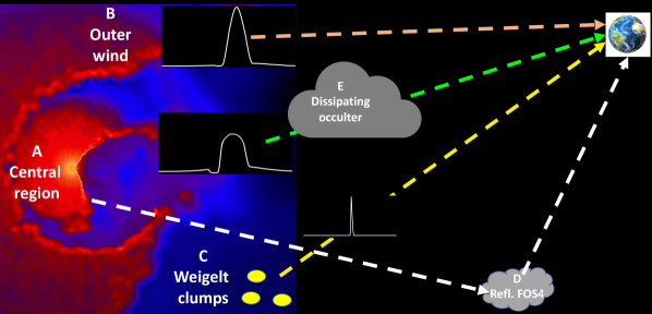
Figure 1: Scheme showing the five main components of the $\eta$ Car spectrum. The $\eta$ Car image is a snapshot from a 3D simulation by Madura et al. (2013). The structures are not to scale.

The FOS 4 region at the SE pole of the Homunculus is located at 4^′′ from the central stellar core (Davidson et al., 2005). This region receives mostly unobstructed light from the central object (see the darker line in the upper plot of Fig. 2), with a spectrum that is typical for an LBV star, with no significant contribution from narrow-line components. Its spectrum was taken with the UVES spectrograph in 2006.5 (seeing-limited, ground-based observations) and has remained very stable since then (see Fig. 4 from Damineli et al. 2021). A coeval spectrum was also taken with UVES in direct view, indicated as the red spectrum in Fig. 2. The year 2006.5 corresponds to the mid-cycle of the $\eta$ Car system ($\phi\,=\,0.52$) and fairly represents its high-excitation phase. The wavelength range was chosen to show lines from representative ionic species. The direct view of the star is attenuated by the (semi-transparent) occulter, which diminishes the flux originating from the central region, increasing the strength of narrow lines relative to the stellar continuum, from the perspective of the observer. Gull et al. (2023) suggest that the occulter is located at $\approx$ 1000 au from the central star and was ejected around 1890.

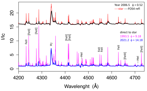
Figure 2: Ground-based (seeing-limited) high-resolution spectra of $\eta$ Car. Upper panel: The thick black line at the top shows the spectrum reflected off the Homunculus at the FOS 4 position, observed in 2006.5. It represents an unobstructed view of the system. H$\alpha$ emission profile in reflected light has been decreasing by a much smaller amount than in direct light and other emission lines have not changed. The thinner red line shows a coeval spectrum in direct view toward the central star (presumably impacted by the occulter). Bottom panel: direct view spectra taken in 1993.5 ( orbital phase 0.18) with the FEROS spectrograph (thin pink line) and 2021.2 (same phase), taken with LCOGT/NRES (thick blue line). A broad base on many of the Fe ii lines is readily apparent. The direct spectrum has evolved towards that reflected at FOS 4, which has evolved by a small amount.

As the occulter dissipates with time, the spectrum becomes more similar to that of the reflected view, as shown by comparing the pink line in the bottom plot of Fig. 2, taken in 1993.5 using ESO/FEROS, with the overplotted blue spectrum taken in 2021.2 with LCOGT/NRES.)

The effect of the occulter on the line strength is strongly dependent on the radial density profile of the line-formation zone plus the size, geometry, and radial opacity profile of the occulter. An approximation of the stellar wind structure can be inferred from the model of Hillier et al. (2001a, see their Fig. 9). Broad Fe ii lines are formed in the outer regions of the primary’s wind. Their intensities relative to the continuum have been decreasing with time at a slower pace than the narrow lines formed in the Weigelt clumps. The broad forbidden [Fe ii] lines are formed at typically larger radii than the permitted Fe ii lines. In addition, their strength (normalized to the continuum) has also decreased by a significant factor from 1993.5 to 2021.2, as indicated in the bottom panel of Fig. 2. During the same period (1993.5–2021.2), the narrow-line fluxes (normalized line strength times the continuum flux) remained constant (Damineli et al., 2021).

Higher energy excitation lines (e.g., He i, N ii and high members of the H i line series) are formed close to the central star, and some of them are entirely covered by the occulter. For instance, the H ${\gamma}$ line shown in Fig. 2 has not significantly changed over the last 28 years, while the EW of H$\alpha$ has decreased by a factor of $\sim$2. High-excitation permitted lines formed behind the occulter would maintain their normalized intensity if there was no emission from outside the occulter. However, the wind region emits both continuum (bound-free and free-free radiation, and electron scattering) plus line emission, and this can veil absorption lines. Further, if the occulter extinction is large enough, the observed spectrum will be dominated by the spectral formation in the region outside the occulter. As the flux from the occulted region increases (when the extinction decreases), the contribution from the central region increasingly dominates, making the absorption lines more visible.

The presence of the hot secondary star complicates this simple scenario, as it affects both the primary wind structure and its ionization (e.g. Mehner et al., 2012, 2011). For most of the orbit, the higher-order Balmer lines do not exhibit a (strong) P Cygni absorption component, which is directly attributable to the influence of the secondary (Groh et al., 2012b). However, strong P Cygni absorption just after periastron (i.e., when the companion is behind the secondary and the trailing arm of the wind-wind collision structure is in the line-of-sight) have been reported by Nielsen et al. (2007) and Mehner et al. (2015).

The goals of this work are $a)$ to report the long-term evolution of the P Cygni absorption components as seen from ground-based spectroscopy; $b)$ to discuss how the strengthening of the absorption components and the weakening of the emission line components compare with models of decreasing mass-loss rate and with a dissipating occulter in front of $\eta$ Car.

This paper is organized as follows. In Sect. 2, we present the sources and general characteristics of our data; in Sect. 3, we present the measurements and their analysis; in Sect. 4, we report cmfgen modeling with normal and enhanced mass-loss rate and two versions of occulter. Sect. 5, we discuss our findings.

2 Data: observations and reduction

Table 1: Observatories

Observ.	telesc.	Res.	5876	6347	8750	10830
	aper.	pow.	#	#	#	#
UVES	8m	90K	1	62	28	-
GMOS	8m	4.4K	22	22	-	-
FEROS	1.5&2.2m	48K	186	169	141	-
OPD	1.6m	22K	25	73	32	140
Hexapod	1.5m	48K	8	-	-	-
CHIRON	1.5m	90K	80	246	-	-
SMARTS	1.5m	40K	91	83	-	-
NRES	1m	48K	102	102	102	-
HERCULES	1m	48K	9	14	8	-
M. Johnston	0.60m	17K	-	5	-	-
P. mcGee	0.35m	11K	1	7	-	-
P. Cacella	0.30m	5.5K	13	-	-	-
K. Harrison	0.28m	10K	-	5	-	-
B. Heatcote	0.28m	16K	10	26	-
T. Bohlsen	0.27m	15K	3	12	-	-
G. Di Scala	0.20m	17K	-	2	-	-
STIS	2.5m	10K	-	-	-	-

Column 1 is the spectrograph/observer name; col. 2 the telescope aperture in meters; col. 3 the most frequent resolving power; col. 4–7 the number of measurements used in this work.

For the modeling, and considering we are interested in looking at the general behavior of line strengths, it is sufficient to have two or more spectra taken at the exact same orbital phase over a time interval long enough to enhance the emission weakening and absorption strengthening effects. For the emission lines, it is already proven that there is a weakening trend in the long-term (Mehner et al., 2015; Damineli et al., 2021). For the P Cygni absorptions, however, the past reports are confined to at most three cycles (Mehner et al., 2015) and are better sampled around periastron. The fluctuations are large even at mid-cycle, so the idea that they are strengthening over many cycles is not completely stabilished. To show this, we require dense monitoring over as many cycles as possible. The most practical quantity to use for such a time series is the equivalent width (EW).

The data used to measure EWs in this work are mainly from the facilities described in Damineli et al. (2021). We list those facilities in Table 1 and, for details, we direct the reader to Sect. 2 of Damineli et al. (2021). In addition to the professional facilities, there are a few observations from amateur astronomers – these also listed in Table 1 and partly described in Teodoro et al. (2016) (also see the Acknowledgments).

Most of the spectra obtained from other authors and observatories were in 1D format (in counts versus $\lambda$), reduced with standard procedures. They are seeing-limited ($>$ 1”), and since most of the signal from the object originates in the central arcsec, these spectra sample similar nebular contamination. Data from ESO/UVES and Gemini/GMOS, downloaded as 2D images from the Treasury Project, were used to extract 1D spectra using all the spatial rows along the slit containing the stellar signal to mimic the worse image quality of the other observations which used a slit (1” wide) or fiber ($\sim$3” diameter). Even in the case of excellent seeing, when some contribution to the signal from the Weigelt clumps could be left outside the slit aperture, they impact only the narrow-line components, and this work is concerned with the broad components, originating in a smaller region. The two HST/STIS 2D spectra were downloaded from MAST site. To avoid as much as possible contamination by the Weigelt clumps in STIS spectro-images, we co-added five rows around the peak of the stellar image (0$\farcs$25-wide). Typical signal-to-noise ratios (S$/$N) of the ground-based spectra range between 60 and 300 in the central region, with the most frequent value $\sim$150. On average, the lowest S$/$N was observed for the P Cygni absorption component of He i $\lambda$10830 line, with S/N$\sim$ 80 to 100 per pixel. This is because we use normal CCDs with very low quantum efficiency at those wavelengths ($\sim$ 1-2%) and a large impact because of fringing and telluric lines. Despite $\eta$ Car being a very bright source at that wavelength, observation of a telluric standard star is required. Other time-consuming procedures are applied in the flat-fielding to maximize the final S/N, demanding a few hours to get a reliable spectrum.

Spectra spanning a wide wavelength range were normalized to unity by dividing them by a high-order polynomial fit through line-free spectral windows representing the stellar continuum. This procedure was mostly used for visualization purposes like that presented in Fig. 2. A linear fit was used for estimating the continuum by adopting line-free regions for spectral ranges shorter than $\sim$ 100Å.

For EWs of absorption components, we fitted a straight line representing the continuum across each spectral line. Two windows were chosen, one at each side of the line, spanning sixteen pixels. For He i $\lambda$5875 the continuum windows are centered at $\lambda$5851 and $\lambda$5930; $\lambda$6329 and $\lambda$6400 for Si ii $\lambda$6347; $\lambda$8722 and $\lambda$8770 for H i $\lambda$8752; $\lambda$10760 and $\lambda$11000 for He i $\lambda$10830. The S$/$N ratio of the continuum was measured inside the two continuum windows. The real S$/$N of the EW is lower for the absorption and higher for the emission, because were measured in the continuum windows.

EWs were measured by direct integration in the area between that line profile and the projected stellar continuum. The uncertainty of individual EW measurements ($\sigma_{\rm EW}$) was evaluated using Eq. (3) from Vollmann & Eversberg (2006), given by:

$$\sigma_{\rm EW}=\sqrt{2}\cdot\left(\frac{\Delta\lambda-\rm{EW}}{\rm{S/N}}\right)$$ (1)

where $\Delta$$\lambda$ is the wavelength interval used to integrate the flux (in Å). Eq. 1 also accounts for the influence of small-scale irregularities and possible faint lines in the continuum window. EW measurements with respective errors are reported in Appendix 2, and presented in Fig. 6.

For our high-quality spectra, the largest uncertainties might not be due to photon statistics, but rather arise from the procedures of continuum flattening and the bias introduced by the nebular contribution which will not be identical for each spectrograph. The only way to evaluate these uncertainties is by comparing the coeval series of measurements taken with different spectrographs. We did this for the epochs for which it was possible compare measurements of at least two spectrographs. Only the EWs from the line Si i $\lambda$6437 had overlaps between different spectrographs that were frequent enough for this procedure. Unfortunately, the EW curve for this line is very complicated, with large variations within a couple of months. The scatter inside each data-sample was larger than the differences between its average curve and the other group used to compare with it. So, no relative shifts were applied for any EW groups.

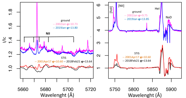
Figure 3: Comparison of spectral evolution obtained from HST/STIS spectra taken at phases 10.60 and 13.64, and ground-based spectra taken at 10.73 and 13.80. The broad emission components show similar weakening in space and ground-based data, as also is the absorption strengthening in He i $\lambda$5875 (right panel). Narrow emission affects more the ground-based spectra but also fills most of the N ii absorption P Cyg components (left panel). N ii $\lambda$5710 is almost free of contamination in space and ground-based spectra, showing similar time-strengthening behavior in both datasets. Extraction in a lower number of rows could lead to less contamination in STIS spectra, but this would have demanded much longer exposures to achieve a high signal-to-noise ratio.

Line strengths were measured as follows: $a)$ the line depth intensity was measured directly at the minimum of the P Cygni absorption component relative to the stellar continuum and reduced by subtracting 1 (negative strength); $b)$ the peak of broad emission lines was deblended from the narrow component by a double Gaussian fit (narrow plus broad components) and the peak of the broad component is the peak of the broader Gaussian. This peak also was subtracted by the continuum (set at 1.0). This method was applied to pairs of 1993.5 and 2021.2 ground-based spectra and 2001.4 and 2018.2 STIS spectra.

3 Results

Previous studies of P Cygni absorption variations on He i $\lambda$6678 line (Mehner et al., 2010, 2012), He i $\lambda$4713 and N ii $\lambda$4601-46743 (Mehner et al., 2015) have been limited to three orbital cycles. Here, we examine a larger number of spectral lines with a denser and longer time-sampling to monitor the spectral evolution in the optical window, using ground-based observations.

The absorption components exhibit four types of variability: a) variability in the depth of the P Cygni absorption components around periastron; b) variations along the orbital cycle due to changes in the distorted shape of the primary star’s wind caused by the WWC cavit – In most of the lines, these variations have a relatively low amplitude when compared to the low-excitation event around periastron; c) episodic low-amplitude variations near mid-cycle, lasting from days to months; d) continuous, smooth, long-term low-amplitude modulation.

The events caused by periastron passage are easily identifiable by the strong peaks in the EW curves – the most noticeable variations start ten days before phase zero and last for about three months – see Fig. 6. These events are characterized by an increase in the radial velocities of the absorbing components beyond the terminal wind speed of the primary star (420 km s^-1; Groh et al., 2012a) - see Fig. 5.

Episodic variations are difficult to identify as they require frequent monitoring of the EW over long time scales (years). They do not show changes in the velocity of the line profiles in absorption at mid-cycle. We identify those sporadic variations by analyzing the time series after subtracting the long-term trend.

Long-term variations in absorption lines can be gleaned by comparing spectra taken at the same phase in high-excitation phases, in different orbital cycles, as such variations are generally larger than the sporadic low-amplitude variations. The long-term increase in the strength of the P Cygni absorption component is easy to see in some lines, such as He i $\lambda$10830, but more difficult in other lines such as He i $\lambda$5875 and H i Pa12 $\lambda$8752.

Our planned modeling of the spectral evolution is based on comparison of line profiles of two spectra taken at the same phase, sufficiently separated in time as to have clear differences. To validate this approach and the selection of the specific dates we follow three steps. First we compare STIS spectra with ground-based spectra to show that they deliver compatible results, at least for the very rare dates when this is feasible. Second, we compare ground-based line profiles of spectra taken at the same phases in different cycles to show that the strengthening of the P Cygni absorption is a general property of of the spectral evolution. Third, we construct long time series of EWs, to see what phases are most repeatable, except for the long term effect.

3.1 Are ground-based spectra comparable to STIS spectra to study long-term spectral evolution?

Although the ground-based spectra have much more nebular contamination than the STIS spectra, both data sets display a similar spectral evolution. This can be shown by comparing the evolution in STIS spectra that were taken at the same phase during the high-excitation state, with the evolution in ground-based spectra, shown in Fig. 3. For this exercise, we use STIS observations that were taken at $\phi\,=\,10.60$ and 13.64. while the almost coeval ground-based spectra were taken at phases 10.7 and 13.80. The exact amount of line variation is not important here. The right panel of Fig. 3 shows that the P Cyg absorption in He i$\lambda$5875 increases with time in both STIS and ground-based spectra while [N ii]$\lambda$5755 and NaD complex decrease. The left panel shows the faint lines of N ii. The group member at $\lambda$5712 shows a small degree of increase with time. The other four members also show the same trend of increase but are contaminated by nebular emissions. We tried to diminish the length of the extraction window to 0$\farcs$1 to improve the situation, slightly reducing the central peak of the $\lambda$5776+5680 blend, but at the expense of decreasing the signal-to-noise ratio. This set of N ii lines was reported by Mehner et al. (2011), who also analyzed a STIS spectrum. They are much more evident than in the spectrum we present here. The reader must take in mind that that spectrum was taken only five months after periastron passage, when the absorption lines are stronger, with a much longer time exposure and adopting a smaller( 0$\farcs$1) extraction window, leaving almost all the nebular contamination outside the slit aperture.

To confirm the trend of strengthening of the absorption in this line, we call attention to the report made by Davidson et al. (2015), who examined another set of N ii lines in the range $\lambda$4601-4643 Å. They were not evident in 2003.3 and 2009.0, but appeared as stronger absorption features in 2014.5. Those lines are stronger than in 2014.5, even in ground-based spectra taken during the 2020 periastron. Such a comparison indicates that ground-based spectra show similar trends to those observed from STIS observations, even in a challenging situation like in the P Cygni absorption of N ii. This study validates our choice for using the ground-based spectra because they comprise many cycles with a better time sampling of the mid-cycle phases.

3.2 Comparison between line profiles taken at the same phase in different orbital cycles

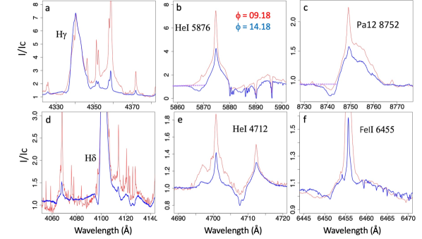
Figure 4: Representative line profiles at $\phi$ =9.18 – June 1993 (thin red lines) and $\phi$ =14.18 – March 2021 (thick blue lines), showing the increase in P Cygni absorption over the 28-year time interval and a decrease of (almost all) emission lines at mid-cycle. Also evident is the dramatic weakening of the narrow nebular lines, and the broad base associated with forbidden and permitted Fe ii lines. For flux-calibrated spectra, see Fig. 2 of Damineli et al. (2021). Horizontal dotted lines in panels $b$ and $c$ indicate the continuum used for EW absorption measurement.

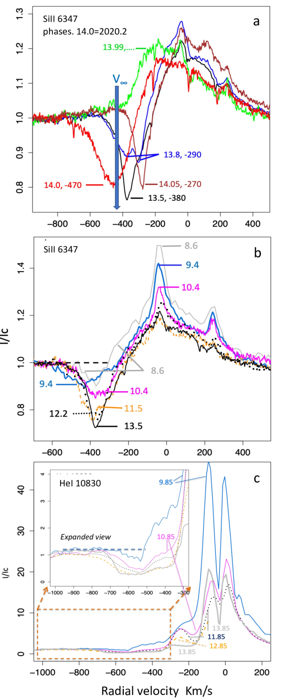
Figure 5: Line profiles of Si ii $\lambda$6347 (panels a and b) and of He i $\lambda$10830 (panel c). The inset in panel b displays an expanded view of the absorption profile. Panel a shows variability around periastron. Panels b and c show high-excitation phases. The horizontal dotted line in the inset indicates the adopted stellar continuum used for EW absorption measurements.

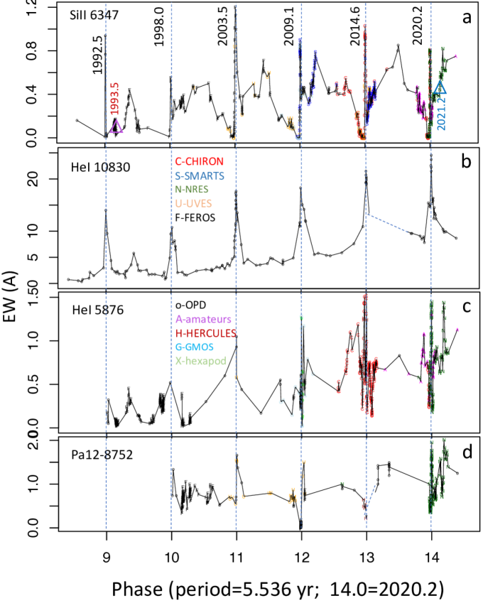
Figure 6: Time series of EWs of the P Cygni component in absorption. a) Si ii $\lambda$6347: this line indicates that variability is complex even at high excitation phases; b) He i $\lambda$10830: strengthens smoothly at high excitation; c)He i $\lambda$5875: although the general trend is of increasing strength, there are occasional oscillations outside of periastron; d) Paschen 12: shows transient variations in the vicinity of periastron. Observations from different facilities are labeled by letters and colors - a zoomed view shows more clearly the letters. The two triangles in the upper panel indicate the dates selected for modeling the spectra - which in reality was replaced by the FOS 4 reflected spectrum which has no narrow lines.

Visual comparison between (a window of) two high-resolution spectra taken 28 years apart (five orbital cycles) are presented at the bottom plot of Fig. 2. The two ground-based spectrographs, ESO/FEROS (at the 1.5$-$m ESO telescope) and LCOGT/NRES (1-m telescope), have equal spectral resolution R $=$ 48,000 and are fiber-fed with projected entrance diameter projected on the sky of $\sim$ 2$\farcs$7. They were taken one year after periastron, the first in June 1993 ($\phi$ $=$ 9.18) and the second in March 2021 ($\phi\,=\,14.18$). At this phase, the spectrum has already recovered from the “low-excitation event”. The 1993 spectrum is representative of what has been called the “$\eta$ Car-like” spectrum.

In the $\phi\,$=$\,9.18$ spectrum, absorption profiles only appeared in lines from very high-excitation levels of the Balmer and Paschen series, in Si ii $\lambda$6347, and in He i lines such as He i $\lambda$4026, He i $\lambda$4712 and He i $\lambda$10830. During cycles 9 and 10, strong absorption components appeared only around periastron passage – see Fig. 5.

The long-term strengthening of P Cygni components affects many other lines. For example, Fig. 4 focuses on line-profile differences at $\phi\,=\,9.18$ and $\phi\,=\,14.18$ for some representative lines. Panel $d$ (bottom left panel) shows that the H$\delta$ line did not exhibit P Cygni absorption at $\phi\,=\,9.18$, but did five orbital cycles later for the same phase. The top-right panel of Fig. 4 $c$ shows that the P Cyg absorption of Pa 12 line - (H i $\lambda$8752) - has strengthened, as was the case for H$\delta$, H$\gamma$, Fe ii $\lambda$6455, He i $\lambda$5875 and He i $\lambda$4712. Panels $b$ and $c$ show a dotted line representing the local stellar continuum used to integrate the EW along the absorption-line profiles.

Some spectral lines, such as Si ii $\lambda$6347 and He i $\lambda$10830, were monitored sufficiently often to allow a comparison of their line profiles over five or six orbital cycles. The top panel of Fig. 5 shows that far from periastron, velocities in the absorption profiles are smaller than the terminal velocity of $\eta$ Car primary’s wind, which is compatible with line formation at smaller radii. From 10 days before to a month after periastron, the profile shows very high speeds, as expected if the trailing arm of the WWC wall passes through our LOS at those times. The middle panel of Fig. 5 shows that the P Cygni component of Si ii $\lambda$6347 at phase 0.4 $-$ 0.6 increases with time. The bottom panel of Fig. 5 shows the same strengthening long-term evolution of He i $\lambda$10830 P Cygni component, in this case at $\phi$ = 0.85. An expanded view of the P Cygni absorption trend is shown in the inset of panel c.

The evolution of these two spectral lines shows that the amplitude of both emission and absorption variations seem to have slowed down in the last three cycles, consistent with the almost complete disappearance of many “circumstellar” absorption lines in the UV (Gull et al., 2021, 2023), and with the disappearance of the blue-shifted narrow absorption of NaD (Pickett et al., 2022).

3.3 EW time series of P Cygni absorption components

The comparison of spectra taken at the same phase in successive cycles is very useful because, in principle, they would be identical if no long-term evolution occurred. However, as we are interested in low-amplitude effects, even minor irregularities in the orbital variations can impact the comparisons. A more panoramic view would be assembling time series in which such irregularities could be identified. The number of spectral lines in which this is possible over five to six cycles is small, especially as only a few lines show an absorption component at mid-cycle. In addition, since the measurements come from different instruments, we had planned to scale the different series in epochs when they are coeval. However, scaling was not necessary in the case of some lines and not possible for others, as seen ahead. The plots of the EW time series (Fig. 6) have the identification of every observational point with a letter indicating its instrumental source - a zoomed view might be necessary to see clearly the individual points.

The EW-curve of Si ii $\lambda$6347 shows an overall long-term increase but with plenty of structures repeated over every orbital cycle (panel $a$ of Fig. 6). We call attention that the mid-cycle maximum does not occur at the exact same phase in every cycle. This exemplifies how careful the choice of dates to examine long-term evolution must be. The crossing of the trailing arm of the WWC causes sharp enhancement of Si ii $\lambda$6347 absorption around periastron passage.

The P Cygni absorption component that has the simplest time variation is that of He i $\lambda$10830, as shown in panel b of Fig. 6. The low scatter of this EW-curve is explained by the large intensity of this feature and, in part, because it is recorded by the same spectrograph (OPD/Coudé) over three decades, although using several different CCD detectors. The EW-curve shows a smooth long-term increase at mid-cycle phases, combined with the usual narrow peaks at periastron.

The He i $\lambda$5875 absorption component strengthens with time, but it exhibits irregularities even at mid-cycle, differently from He i $\lambda$10830 (see the middle panel of Fig. 6). This is due to the contribution of the WWC in this spectral line as shown by Richardson et al. (2016). These variations are even more pronounced at periastron passages and are not strictly periodic. Even so, it is possible to identify a long-term strengthening trend in the mid-cycle from cycle #10 onward. The modulus of the radial centroid velocity of the P Cygni absorption component is $\sim$ 500 km s^-1 at mid-cycle and up to 1000 km s^-1 at periastron – well beyond the terminal speed of the wind – indicating that they are probably produced in the WWC walls and are subject to shock instabilities. This finding aligns with the results from Richardson et al. (2016).

Even though measurements of weak lines are subject to large uncertainties, the absorption component of the H iPa12$\lambda$8752 line also strengthens with time, as shown in the bottom panel of Fig. 6. Since this H i line is formed in the innermost parts of the primary’s wind, the emission contribution from radii outside the occulter is smaller than in lower H i transitions. Studying this spectral line is important because it has a permanent and mostly non-blended absorption component.

Table 2: Sample of Tables A.1 – A.4 in online material

HJD	EW 5875	$\sigma_{\rm{EW}}$	Facility
	(Å)	(Å)
48793.994	0.18	0.09	OPD/Coudé
48830.020	0.07	0.06	OPD/Coudé
48838.996	0.05	0.04	OPD/Coudé
48843.988	0.32	0.06	OPD/Coudé
49063.609	0.05	0.04	ESO/FEROS

HJD	EW 6347	$\sigma_{\rm{EW}}$	Facility
	(Å)	(Å)
47918.500	0.16	0.03	OPD/Coudé
48780.500	0.01	0.00	OPD/Coudé
48793.990	0.94	0.19	OPD/Coudé
48798.500	0.77	0.15	OPD/Coudé
48825.010	0.04	0.01	OPD/Coudé

HJD	EW 10830	$\sigma_{\rm{EW}}$	Facility
	(Å)	(Å)
47613.590	0.72	0.12	OPD/Coudé
47916.730	0.54	0.09	OPD/Coudé
48020.800	0.32	0.05	OPD/Coudé
48059.390	0.79	0.13	OPD/Coudé
48255.760	1.00	0.17	OPD/Coudé

HJD	EW Pa-12	$\sigma_{\rm{EW}}$	Facility
	(Å)	(Å)
50833.750	0.74	0.15	OPD/Coudé
50854.583	1.33	0.20	OPD/Coudé
50946.375	0.74	0.15	OPD/Coudé
51131.815	0.33	0.16	ESO/FEROS
51135.819	0.45	0.23	ESO/FEROS

Note. The first five rows of each table are presented. The full version of the table is available online.

The EW time series provides a robust method to study the long-term strengthening of P Cygni absorption features, which was shown in previous reports (Mehner et al., 2010, 2012, 2015), but were restricted to shorter time intervals. EW time series are important to track the long-term evolution of the P Cygni absorption components. Still, many lines exhibit relatively weak features and/or are severely blended with other spectral components. This is why we rely on line peak/depth variation for modeling purposes.

The general evolution pattern of the observed spectrum in the last 30 years is $a$) a strong weakening of the narrow emission lines; $b$) a general weakening of the broad emission line components by 50% for lines formed up to large radii in the wind (low excitation lines) and less for lines of high excitation transitions, formed close to the central stars; $c$) a general strengthening of P Cygni absorption components. This can be seen for representative lines in Fig. 8 (magenta and green lines) and quantitatively (rows $1$ and $2$) of Table 3. In this table, in addition to the line strength (rows 1 to 6), we present the percent difference between spectra (rows 7 to 12), as indicated in column 1. Negative numbers are produced when the line in the first spectrum is weaker than in the second. Numbers printed in red indicate variations in the contrary sense of observations. Differences smaller than 20% are disregarded.

4 cmfgen modeling

The main goal of this paper is to show that the dissipating occulter modulates the strength of the emission and P Cygni absorption strengths in accordance with the observed long-term spectral evolution of $\eta$ Car. Since only the general trend of the $V$-band extinction is available (Damineli et al., 2019), only the relative line strength is useful, not a time series with every single EW measurement. After a careful examination of the time series in Sect. 3, we chose two ground-based spectra taken in 1993.5 ($\phi$ = 9.18) and in 2021.2 ($\phi$ = 14.18) to represent the ratio of the line-strength variation. Other phases in mid-cycle could be used, but 0.18 is the one for which we have the longest time interval - maximizing the spectral evolution - in addition, at this phase – one year after the periastron – we look to the primary star photosphere in a less-disturbed situation than in others (Madura et al., 2013). The WWC trailing arm has already left our LOS, and the cavity is not wholly occupying our view. Line peaks/depths offer a cleaner way than EWs to measure line strength variations as they are less affected by blend effects on the line wings. We call line strength the peak (or depth) of the broad wind lines above (or below) the stellar continuum. These are the quantities we use to compare with the synthetic models and are reported in Table 3.

4.1 cmfgen model of the present-day unosbtructed wind

We used the cmfgen code to calculate a full wind model following (Hillier et al., 2001a, 2006), with the following parameters:
R_∗ $=$ 240 $R_{\odot}$;
$\dot{M}$ $=$ 3.9 $\times$ 10^-4 $M_{\odot}\,\hbox{yr}^{-1}$;
L $=$ 4 $\times$ 10⁶ $L_{\odot}$; and
N(H)/N(He) $=$ 10
This model is similar to that which fitted the infrared interferometry across the Brackett alpha emission line (see Weigelt et al. 2021 and references therein). The N(H)/N(He) ratio was increased from 5 to 10 to better explain the influence of the occulter on the Fe ii lines. In turn, this required a slight reduction of the mass-loss rate from 5.0 $\times$ 10^-4 $M_{\odot}\,\hbox{yr}^{-1}$ to preserve the H/He i spectrum. When a fixed solar mass fraction for iron is adopted, the Fe ii lines are weaker in the model with a high N(H)/N(He) ratio. Qualitatively, the influence of an occulter on a model with N(H)/N(He) $=$ 10 or 5 is not that different. Allowing for the radiation field of the binary companion (Damineli, 1996; Damineli et al., 1997, 2008) would provide an alternative means of weakening the strength of Fe ii emission lines (Groh et al., 2012a).

The modeling of the unobstructed spectrum is complicated by several factors, including:

1. While we have an estimate of the primary’s luminosity (albeit somewhat uncertain due to the unknown efficiency of the conversion of optical/UV light to IR wavelengths and the luminosity of the companion), we do not have a measurement of the intrinsic optical flux emitted by the system at optical and UV wavelengths.

   

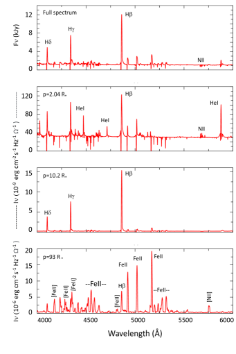
   Figure 7: An illustration of the primary star’s fully integrated spectrum with the specific intensity for different impact parameters, $p$. This parameter is the projected radius inside which the wind is excluded. As can be seen from the figures, the spectra vary strongly with the impact parameter. This variation arises due to radial variations in both ionization and density. In the spectrum for $p\approx 2\,R_{*}$, the He i lines (.e.g., $\lambda 4471$, $\lambda 5876$) line are much stronger than in the stellar spectrum. For $p\approx 10\,R_{*}$ H lines dominate the spectrum, while for $p\approx 90\,R_{*}$, Fe ii and [Fe ii] lines are prevalent. Thus spatial variations in the occulter will have a strong influence on the observed spectrum. Note: If we assume a spherical source, and ignore the occulter, the observed flux is proportional to $\int pI(p)dp$.

2. There is a degeneracy between the mass-loss rate and the H/He ratio, such that similar H and He i spectra can be produced for different mass-loss rates and H/He ratio values (Hillier et al., 2001a). Metal lines, such as He ii, can break the degeneracy, but there are additional difficulties in modeling these lines. For example, in models with a higher H/He ratio, the metal lines are weaker since N(H)/N(Z) is higher (the metals are assumed to have a solar mass fraction).

3. The He i line strengths are most likely affected by the ionizing field of the companion (Nielsen et al., 2007), limiting our ability to use the strength of these lines as constraints. Therefore, in the present modeling, we demanded that the He i lines should be weaker than in the observations.

4. The hotter companion star ionizes the outer wind, affecting the strength of the P Cygni profiles on Balmer lines, with low-series members (such as H$\alpha$) being the most affected. The P Cyg absorption, especially those associated with Fe ii lines, is also affected.

5. The wind is optically thick, so the core radius is challenging to constrain. However, values ranging from 60 to 240 R_⊙ are roughly compatible with the observations. In the present modeling, we adopted 240 R_⊙ since this allowed us to get a reasonable match to the higher Balmer series members without having too much He i emission. Note: At a small core radius, the wind dominates the formation of the optical spectrum, but as we increase the radius, the influence of the wind declines, and the shape of the visual continuum changes.

6. If the primary associated with $\eta$ Car is a fast rotator, there could be significant asymmetries as suggested by (Smith et al., 2003a). However, direct spectra taken of the central star, and those using the reflected light seen at FOS 4 are now much more similar than in the past.

7. The occulter may still be influencing (albeit more weakly than in the past) the ground-based spectra. Ground-based spectra at FOS 4 are also not clean since the spectra did show some evidence of “scattered” emission from the Weigelt clumps (Hillier & Allen, 1992).

The main effect of the complicating factors is that we cannot develop a well-defined model with realistic error bars. Further, the adopted parameters we selected are generally strongly correlated. However, the parameter space of viable models is limited. Even if some spectral lines deviate significantly from observations, this study can produce valid results by looking at the line ratios calculated in different astrophysical scenarios: variable mass-loss-rate, presence or absence of a coronagraphic occulter.

The unobstructed (full wind) model is named as f.w.($\dot{M}_{\rm low}$) in row #3 of Table 3 and is shown as a black line in Fig.8. It is intended to fit the present-day spectrum, which we adopted as that observed in reflection at FOS 4 (green line) - it is very similar to that of 2021.2, except for having less narrow-line contamination and somewhat deeper absorptions. There is a good match to emission lines, except for He i$\lambda$5875. The broad line component of [Fe ii]$\lambda$4815 is in reasonable agreement with the observation. The excess emission at the peak of the FOS 4 spectrum is a reflection from Weigelt clumps. The full wind models produce P Cygni absorptions stronger than observed. This is a problem not solved in this and previous papers dealing with spectral modeling with cmfgen. It may be due to the before-mentioned peculiarities of $\eta$ Car.

4.2 How a mass-loss rate that decreases with time contradicts the observed spectral evolution

To explore the effect of a larger mass-loss rate in the past, as suggested by other authors (seenDavidson et al. 2018 and references therein) trying to explain the decrease in emission line strengths with time, we consider a model with a mass loss rate of 7.8 $\times$ 10^-4 $M_{\odot}\,\hbox{yr}^{-1}$– twice that of the model that fits the present-day spectrum. All other parameters, including the terminal velocity of the wind, remained fixed. However, LBVs typically show simultaneous changes in both the mass-loss rate and $V_{\infty}$. No evolution in $V_{\infty}$ has been observed in the spectral evolution of $\eta$ Car.

This unobstructed model with a 2$\times$ higher mass-loss rate is hereafter denoted by f.w.($\dot{M}_{\rm high}$). In Fig. 8 the line profiles of the 2$\times$ mass-loss-rate are represented by the thick grey line, and the percent difference with the model for the present-day spectrum – f.w.($\dot{M}_{\rm low}$) – is displayed in the $9^{th}$ row of Table 3.

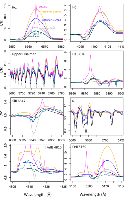
Figure 8: Spectral comparisons between observations and models. Earlier dates are in magenta and later in green. The N ii spectrum was taken with STIS and the others are ground-based. The full wind model (black) is intended to be compared with FOS 4 (unobstructed view) - green - the 2x mass-loss rate (grey) is to be compared with earlier dates; the occulter with 1.6 mag extinction (blue); and the 2.5 mag extinction occulter (orange), both to be compared with earlier dates.

A decrease in mass-loss rate with time mimics the observed decrease in the observed emission-line components of the Hydrogen Balmer but not in the P Cygni components, which are weakening in the model, but remained stable in the observations. There is an acceptable agreement between this mass-loss regime and the 1993.5 spectrum for Fe ii$\lambda$5169, but it predicts a too faint [Fe ii]$\lambda$4815 emission. The emission components in the model f.w.($\dot{M}_{\rm high}$) evolve on the contrary sense to the observations for the lines of He i and N ii. For the absorption lines of Si ii and H i Pa 12, the decreasing mass loss rate also evolves contrary to the observations. Moreover, a decrease in the mass-loss rate is usually accompanied by an increase in $V_{\infty}$, as seen for S Doradus stars (Leitherer et al., 1985; Groh et al., 2009; Hillier et al., 2001a), and it would also change the X-ray light curve contrary to what has been observed in $\eta$ Car (Espinoza-Galeas et al., 2022).

4.3 cmfgen models with obstruction by the occulter

In this sub-section, we explore the effect of an obscuring ”coronagraphic” occulter, which is dissipating or is already dissipated. In general (and assuming the occulter lies outside the spectral formation region) the observed flux is given by

$$F=\frac{1}{d^{2}}\int\int_{\scriptstyle\rm star\&wind}I_{\nu}(x,y)\exp(-\tau_{\nu}(x,y))dxdy$$ (2)

where $I(x,y)$ is the specific intensity of the source and $\exp(-\tau_{\nu}(x,y))$ allows for the effect of extinction. For a single star $I_{\nu}(x,y)$ would be azimuthally symmetric on the sky, but the wind-wind collision zone, and the influence of the radiation field of the secondary, will break this symmetry. The substantial variation of $I_{\nu}$ with the impact parameter $p$ is shown in Fig 7 (which defines the projected internal radius of the excluded wind flux). Unfortunately, for the choice of $\tau_{\nu}(x,y)$ we have a wide degree of freedom. The extinction may not be uniform, and may not be centered on the star. However, for simplicity in the paper we limit ourselves to uniform occulters that are centered on the star.

We aim to compare the spectrum of the occulter model with that of the full wind model. We start with the full wind model and subtract from it the spectrum of the region obliterated by a disk. The amount subtracted is defined by the disk size and extinction. We assume that the disk has already dissipated (zero extinction) so that the extinction in 1993.5 is the magnitude difference measured for the entire object (central stellar core plus the Homunculus). The object in 1993.5 was $\Delta$ V $=$ 1.6 mag fainter than in 2021.2 and hence $A_{V}$ = 1.6 mag (Damineli et al., 2019). We adjusted the radius of the occulter’s disk (r $=$ 22.7 R_star) to produce a good match to the observed H$\alpha$ line profile in 1993.5. The distance of the occulter from the central star cannot be assessed in this work, so we adopted that suggested by Gull et al. (2023): $d$ $\approx$ 1000 au, formed around 1890 in the same ejection event as the Little Homunculus.

The occulter models are intended to fit the spectrum taken in 1993.5. Although the occulter1.6 model did a good job for H$\alpha$, the upper Balmer emission lines and He i$\lambda$ 5875 are fainter than observed in 1993.5, and the P Cygni absorptions are stronger than predicted. Both occulter models are broadly compatible with [Fe ii]$\lambda$4815 but their predictions are too strong for Fe ii$\lambda$5169 as compared with observations on 1993.5.

The impact of the occulter on the spectrum cannot be guessed – it requires a calculation using a realistic model. The complications are many: the occulter is unlikely to be disk causing uniform extinction, and may not be centered on the star. As different transitions originate in different regions of the wind, the impact of the occulter is transition dependent. Further, there is significant free-free emission from the wind which will also be influenced by the occulter.

Table 3: Line strengths: observations versus models

		Emission profiles							Absorption profiles
#	Spectral lines	FeII	H$\alpha$	H$\delta$	FeII	[FeII]	HeI	SiII	H$\delta$	HeI	Pa$-$12	SiII	NII
	observations
		8610	6563	4101	4585	4815	5876	6347	4101	5876	8752	6347	5712
1	1993.5	4.6	61	4.5	0.8	0.8	1.9	0.36	0.00	0.00	$-$0.07	$-$0.05	$-$0.04
2	FOS4	1	31	2.5	0.4	0.4	1.65	0.25	$-$0.20	$-$0.45	$-$0.24	$-$0.21	$-$0.06
	models
3	f.w.($\dot{M}_{\rm low}$)		38	2.7	0.35	0.08	0.95	0.28	$-$0.95	$-$0.50	$-$0.40	$-$0.05	$-$0.32
4	f.w.($\dot{M}_{\rm high}$)		55	4.7	1.00	0.09	0.37	0.22	$-$0.85	$-$0.49	$-$0.55	$-$0.44	$-$0.07
5	occulter1.6		66	3.2	1.25	0.23	0.86	0.21	$-$0.90	$-$0.50	$-$0.46	$-$0.16	$-$0.17
6	occulter2.5		135	4.4	3.5	0.42	0.73	0.45	$-$0.36	$-$0.49	$-$0.20	$-$0.05	$-$0.12
% diff.	comparison
(2$-$1)/2	FOS4:1993.5	$-$360	$-$97	$-$80	$-$100	$-$100	$-$15	$-$44	100	100	71	76	33
(3$-$2)/3	f.w.($\dot{M}_{\rm low}$) :FOS4		18	$-$11	$-$14	$-$900	$-$74	11	79	$-$28	40	$-$320	81
(3$-$4)/3	f.w.($\dot{M}_{\rm low}$):f.w.($\dot{M}_{\rm high}$)		$-$45	$-$74	$-$254	$-$13	61	21	11	2	$-$38	$-$780	78
(3$-$5)/3	f.w.($\dot{M}_{\rm low}$):occulter1.6		$-$74	$-$19	$-$257	$-$188	9	25	5	0	$-$15	$-$220	0
(3$-$6)/3	f.w.($\dot{M}_{\rm low}$):occulter2.5		$-$255	$-$63	$-$900	$-$425	23	$-$61	62	6	50	0	63
(6$-$5)/6	occulter1.6:occulter2.5		$-$640	$-$38	$-$260	$-$83	15	$-$114	60	6	65	69	50

Notes: a) The line strength is defined by ($I/I_{c}-1$) at the line peak or deep, negative $=$ absorption, positive $=$ emission; b)f.w. $=$  full wind; c)$\dot{M}_{\rm low}$ = 3.9 $\times$ 10^-4 $M_{\odot}\,\hbox{yr}^{-1}$, $\dot{M}_{\rm high}$ = 7.8 $\times$ 10^-4 $M_{\odot}\,\hbox{yr}^{-1}$, occulter $=$ f.w.($\dot{M}_{\rm low}$) - see the main text; d) % differences: positive $=$ the second is stronger;, negative $=$ the second is weaker). For N ii we used dates 2001.1 and 2019.1. Red figures indicate line strength ratios against the observed trend.

Between 1993.5 and 2021.2 the central star has increased in brightness by $\Delta\,A_{V}\,$=$\,2.5$ mag, in order we consider a model where we increase the extinction in the core by 2.5 mag, but keep the same sized occulter. However, this model is unacceptable – it delivers a H$\alpha$ line intensity that is quite too strong. Keeping the same extinction, we then diminished the size of the coronagraph, obtaining $I/I_{c}-1\,=\,135$ which is much higher than the observed value 61 in 1993.5, but not absurd. A disk with r = 10 R_star produced a good match to H$\delta$ and the upper Balmer series emission, although H$\alpha$ is still too strong. The Si ii$\lambda$ 6347 is in reasonable agreement for the emission and absorption component. N ii$\lambda$ 5712 came better than in occulter1.6 model (occulter’s extinction $=$ 1.6 mag), but still too strong. No agreement was found for He i$\lambda$ 5875 emission. We call this model occulter2.5. As a general comparison, occulter2.5 produces stronger emission and weaker absorption than occulter1.6 (see row 12 in Table 3 and orange line in Fig. 8).

Future work could combine these two models with a radial profile of extinction, decreasing from the center to the periphery. However, designing a completely different geometry may be necessary, as Gull et al. (2023) shows extended patterns of narrow absorption lines in the UV, and Falcke et al. (1996) reported a knife-edge structure crossing over the central star in the polarization map.

Table 3 offers a global comparison between observations versus models and between models. Row 7 shows observed variations that are negative for the emission profiles (weakening) and positive for absorptions (strengthening). Rows 9 to 11 show differences in models that should follow the same trend as in row 7, if they do not agree with observational trends, they are printed in red. Variations smaller than 20% are disregarded. The occulter models with extinction 1.6 disagree with the observational trend in 2 cases and that with 2.5 magnitudes in one case. The 2x mass-loss rate model performed worse than the occulter models to explain the emission line weakening (four cases). Although a complete comparison over the entire spectrum would be more informative (if we had fine-tunned models), this set of lines representative of high and low excitation energies validates the occulter models for explaining the long-term evolution. Although performing worse than the two cmfgen occulter models, the decreasing mass-loss rate model cannot be completely ruled out on the basis of spectroscopy alone.

5 discussion and conclusions

We have used spectral data taken over 30 years to monitor the long-term evolution of $\eta$ Car’s spectrum. In particular, we have studied EW time-series of P Cygni absorption components of He i $\lambda$5875 He i $\lambda$10830, Si ii $\lambda$6347, and H i Pa12 $\lambda$8752.

Some spectral lines like He i $\lambda$5875 and He i $\lambda$4712 suffer non-periodic fluctuations (Richardson et al., 2015; Mehner et al., 2015) even outside periastron. Our ability to distinguish periodic and sporadic variations from long-term variations is enabled by the large amount of data analyzed and because of the significant spectral evolution that has occurred over the last three decades.

We summarize the observational results from the present work, which support the scenario of a dissipating occulter in front of $\eta$ Car A:

• Absorption P Cygni components of a set of representative lines (e.g.: upper members of the Balmer series, He i $\lambda$5875, He i $\lambda$10830, Si ii $\lambda$6347, N ii $\lambda$5665-5712, H i $\lambda$8752 ) have been strengthening with time.

• P Cygni absorption components are deeper in reflected than in direct light at high excitation phases, indicating that the stellar wind formed close to the central star suffers additional extinction along our LOS (by the occulter).

• As the long-term evolution progresses, emission and absorption lines in direct view become more similar to those reflected in the Homunculus (FOS 4 position), which has decreased much less than in direct light in H$\alpha$ emission and remained constant for other lines.

• Emission lines that are formed at larger radii from the star (e.g., H$\alpha$, Fe ii) show a stronger decrease in their line strength than those formed at smaller radii (e.g., the upper members of the Balmer and Paschen series). Lines formed at very small radii like N ii and to some extent He i suffer much smaller line strength changes because the spectral line and its stellar continuum are confined in the same region and change together.

• The observed constancy of the central star while the brightness of the Homunculus increased by $\sim$1 mag during the 1940s (Thackeray, 1953; O’Connell & S.J., 1956), indicates that the occulter was already in place at that time. The photometric light curve of the stellar core since before that time could be dominated by the occulter’s dissipation.

• The rate of decreasing in the emission line intensity and increasing in the absorption maximum/minimum taken at the same phases (see Fig. 5) seems to be decreasing slowly with time, indicating that the occulter’s dissipation might be already ended or is close to ending. The approaching end of the dissipating process is also hinted by the similarity between the reflected spectrum at FOS 4 and the present-day direct spectrum as shown in Fig. 2.

• Although the occulter models examined in this work did not fit all the spectral lines adequately, their percent differences with the full wind evolve in time in the same sense as in observed spectra taken between 1993.5 and 2021.2 in this set of lines (except for Si ii$\lambda$6347). A refinement of the occulter’s structure is likely to give better agreement with observations.

• The decrease in mass-loss rate as the primary explanation for the spectral evolution of $\eta$ Car is not strongly supported by the cmfgen models. It can be rejected because implies in intrinsic changes in the primary star (i.e., changes in terminal wind speed, in the luminosity, in the X-ray light curve, and in the reflected spectrum, at FOS 4) contrary to observations.

From the Weigelt blob constanc, we know that the occulter provides extinction on scales of less than 0$\farcs$1 and the occulter should have a smaller radius. Given that H$\alpha$ emission peaks around 0$\farcs$01, and Fe ii and [Fe ii] emission at even larger radii, it is not unreasonable to assume that differential reddening could influence the EW of absorption and emission lines in the spectrum of $\eta$ Car, as we have demonstrated in this paper. We speculate that the occulter could be similar to the Weigelt clumps, as it is massive and small and might have formed in the same event. We did not identify narrow emission lines of the occulter, probably because they are at our LOS, differently from the Weigelt clumps which show us their ionized borders. Or it is just an effect of smaller density?

The importance of the occulter has greatly diminished during the lifetime of the HST. Since 1993. The visual and UV brightness has increased by roughly a factor of 10. The increased UV brightness has led to an enhanced ionization of the circumstellar material surrounding $\eta$ Car, and as a consequence the disappearance of many narrow absorption lines (Gull et al., 2023). The increase in visual brightness by a factor of 10 has caused the EW of emission lines arising in the Weiglet blobs to be reduced by a factor of 10, making them much less visible in the ground-based spectra. Broad forbidden lines of Fe ii have also been greatly reduced in strength. As this brightening has occurred, the direct spectrum has become much more similar to that seen in reflected light (Mehner et al., 2015; Damineli et al., 2021). It is possible that the occulter has almost dissipated (at least along our LOS). In principle, the reddening to $\eta$ Car should then approach that of the Weigelt blobs.

If the spectral evolution is due to a circumstellar cause, the photometric light curve must be reviewed. Damineli et al. (2021) claim that the brightening of the star in the last 30 years was due to the decreasing circumstellar extinction. At first glance, the long-term photometric light-curve variability after the 1900s looks contrary to the prediction of a stellar merger (see Fig. 2 of Schneider et al. 2019) since it predicts a slow decrease of bolometric luminosity as compared to the rapid increase in $\eta$ Car brightness in the last 30 years. However, suppose these variations are driven by changes in the circumstellar medium, as suggested by the dissipating occulter. One additional test would be the disappearance of HCN molecular absorption in front of the star, reported by Bordiu & Rizzo (2019) using ALMA.

In that case, the star is much more constant than claimed before and would indicate a dormant LBV, like the other non-S Dor variable LBVs, including P Cygni, HD 316285, and HD 168625. In this context, there is no contradiction between the $\eta$ Car light curve and the binary merger scenario as shown by Schneider et al. (2019). In this scenario, the recovery from the Great Eruption of the 19^th century occurred rapidly, on a timescale of less than a century.

6 Data Availability

The complete versions of Tables 1-4 are available in the online journal in a machine-readable format following the CDS/Vizier standards.

7 Acknowledgments

We thank D.S.C. Damineli for adapting our plots to color-blind people. AD thanks to CNPq (301490/2019-8) and FAPESP (2011/51680-6) for their support. The work of FN is supported by NOIRLab, which is managed by the Association of Universities for Research in Astronomy (AURA) under a cooperative agreement with the National Science Foundation. AFJM is grateful for financial aid from NSERC (Canada). This work is partially based on observations collected with the facilities listed below. DJH gratefully acknowledges support from STScI grants HST-AR-14568.001-A and HST-AR-16131.001-A. CMPR acknowledges support from NATA ATP grant 80NSSC22K0628 and NASA Chandra Theory grant TM2-23003X.

Based on observations collected at the European Southern Observatory, Chile under Prog-IDs: UVES: 60.A-9022(A), 70.D-0607(A), 71.D-0168(A), 072.D-0524(A), 074.D-0141(A), 077.D-0618(A), 380.D-0036(A), 381.D-0004(A),282.D-5073(A, B, C, D, E), 089.D-0024(A), 592.D-0047(A, B, C). The first three programmes were described in Stahl et al. (2005) and the others in Mehner et al. (2015); FEROS (partial list): 00.A-0000(A), 69.D-0378(A),, 69.D-0381(A), 71.D-0554(A),079.D-0564(C), 079.A-9201(A), 081.D-2008(A), 082.A-9208(A), 082.A-9209(A), 082.A-9210(A), 083.D-0589(A), 086.D-0997(A), 087.D-0946(A),089.D-0975(A), 098.A-9007(A). Spectra can be downloaded from the ESO database by using the instrument name (UVES or FEROS) plus the Julian Date provided in the Appendix Tables.

Based on observations made at the Coudé focus of the 1.6-m telescope for the Observatório do Pico dos Dias/LNA (Brazil).

Based in part on data from Mt. John University Observatory: MJUO -University of Canterbury - New Zealand).

Based in part on observations obtained through NOIR Lab (formerly NOAO) allocations of NOAO-09B-153, NOAO-12A-216, NOAO-12B-194, NOAO-13B-328, NOAO-15A-0109, NOAO-18A-0295, NOAO-19B204, NOIRLab-20A-0054, and NOIRLab-21B-0334. This research has used data from the CTIO/SMARTS 1.5m telescope, which is operated as part of the SMARTS Consortium by RECONS (www.recons.org) members Todd Henry, Hodari James, Wei-Chun Jao, and Leonardo Paredes. At the telescope, observations were carried out by Roberto Aviles and Rodrigo.

Based on observations obtained at the international Gemini Observatory, a program of NSF NOIRLab, which is managed by the Association of Universities for Research in Astronomy (AURA) under a cooperative agreement with the National Science Foundation on behalf of the Gemini Observatory partnership: the National Science Foundation (United States), National Research Council (Canada), Agencia Nacional de Investigación y Desarrollo (Chile), Ministerio de Ciencia, Tecnología e Innovación (Argentina), Ministério da Ciência, Tecnologia, Inovações e Comunicações (Brazil), and Korea Astronomy and Space Science Institute (Republic of Korea).

Based on observations with the NASA/ESA Hubble Space Telescope, obtained (from the Data Archive) at the Space Telescope Science Institute, which is operated by the Association of Universities for Research in Astronomy, Inc., under NASA contract NAS 5-26555. These two observations are associated with programmes 8619 and 15067 - PI K. Davidson - link: https://mast.stsci.edu/search/ui/#/hst

The ESO/UVES and Gemini S/GMOS spectra used in this paper were downloaded from the HST Treasury Project archive at http://etacar.umn.edu/.

We acknowledge with thanks the variable star observations from https://www.aavso.org/ contributed by observers worldwide and used in this research.

Appendix A Extended data tables (online material)

Table 4: Equivalent widths of the 5875 Å absorption feature.

HJD	EW 5875	$\sigma_{\rm{EW}}$	Facility
	((Å))	((Å))
48793.994	0.18	0.09	OPD/Coudé
48830.020	0.07	0.06	OPD/Coudé
48838.996	0.05	0.04	OPD/Coudé
48843.988	0.32	0.06	OPD/Coudé
49063.609	0.05	0.04	ESO/FEROS
49063.609	0.10	0.08	ESO/FEROS
49065.609	0.10	0.08	ESO/FEROS
49066.621	0.10	0.08	ESO/FEROS
49067.605	0.10	0.08	ESO/FEROS
49068.609	0.09	0.07	ESO/FEROS
49069.609	0.10	0.08	ESO/FEROS
49071.613	0.10	0.08	ESO/FEROS
49072.613	0.09	0.07	ESO/FEROS
49073.648	0.06	0.05	ESO/FEROS
49074.625	0.09	0.07	ESO/FEROS
49075.574	0.08	0.06	ESO/FEROS
49076.625	0.09	0.07	ESO/FEROS
49077.590	0.08	0.07	ESO/FEROS
49078.613	0.08	0.06	ESO/FEROS
49079.605	0.07	0.06	ESO/FEROS
49080.605	0.06	0.05	ESO/FEROS
49081.609	0.06	0.05	ESO/FEROS
49082.609	0.09	0.07	ESO/FEROS
49083.598	0.04	0.04	ESO/FEROS
49084.598	0.09	0.07	ESO/FEROS
49085.598	0.09	0.07	ESO/FEROS
49086.605	0.05	0.04	ESO/FEROS
49087.602	0.02	0.02	ESO/FEROS
49088.609	0.06	0.05	ESO/FEROS
49089.621	0.07	0.06	ESO/FEROS
49089.621	0.08	0.06	ESO/FEROS
49090.605	0.03	0.03	ESO/FEROS
49095.590	0.07	0.05	ESO/FEROS
49098.625	0.06	0.05	ESO/FEROS
49098.688	0.07	0.06	ESO/FEROS
49100.605	0.07	0.05	ESO/FEROS
49101.605	0.07	0.05	ESO/FEROS
49102.605	0.08	0.06	ESO/FEROS
49104.617	0.06	0.05	ESO/FEROS
49105.605	0.02	0.01	ESO/FEROS
49106.605	0.05	0.04	ESO/FEROS
49108.602	0.04	0.03	ESO/FEROS
49110.684	0.05	0.04	ESO/FEROS
49110.684	0.07	0.06	ESO/FEROS
49112.680	0.02	0.02	ESO/FEROS
49113.578	0.03	0.03	ESO/FEROS
49118.563	0.03	0.02	ESO/FEROS
49120.676	0.04	0.04	ESO/FEROS
49122.527	0.05	0.04	ESO/FEROS
49122.527	0.05	0.04	ESO/FEROS
49123.637	0.05	0.04	ESO/FEROS
49124.539	0.07	0.05	ESO/FEROS
49125.535	0.08	0.07	ESO/FEROS
49127.617	0.06	0.05	ESO/FEROS
49129.543	0.04	0.03	ESO/FEROS
49130.543	0.08	0.06	ESO/FEROS
49132.625	0.08	0.06	ESO/FEROS
49134.625	0.02	0.02	ESO/FEROS
49134.625	0.03	0.02	ESO/FEROS
49137.645	0.07	0.06	ESO/FEROS
49138.590	0.03	0.02	ESO/FEROS
49395.867	0.17	0.09	ESO/FEROS
49408.532	0.24	0.12	ESO/FEROS
49424.523	0.18	0.09	ESO/FEROS
49448.605	0.28	0.06	ESO/FEROS
49467.564	0.37	0.07	ESO/FEROS
49472.599	0.45	0.09	ESO/FEROS
49514.541	0.27	0.05	ESO/FEROS
49520.612	0.27	0.05	ESO/FEROS
49522.539	0.29	0.06	ESO/FEROS
49525.528	0.28	0.06	ESO/FEROS
49527.526	0.32	0.06	ESO/FEROS
49532.520	0.33	0.07	ESO/FEROS
49534.504	0.32	0.06	ESO/FEROS
49751.220	0.14	0.07	OPD/Coudé
49770.240	0.15	0.08	OPD/Coudé
49786.120	0.14	0.07	OPD/Coudé
49786.120	0.14	0.07	OPD/Coudé
49800.240	0.13	0.07	OPD/Coudé
49800.240	0.14	0.07	OPD/Coudé
49821.230	0.10	0.08	OPD/Coudé
49846.040	0.09	0.07	OPD/Coudé
49860.070	0.07	0.06	OPD/Coudé
50120.783	0.05	0.04	ESO/FEROS
50146.869	0.05	0.04	ESO/FEROS
50160.749	0.05	0.04	ESO/FEROS
50174.758	0.10	0.08	ESO/FEROS
50188.813	0.06	0.05	ESO/FEROS
50201.733	0.06	0.05	ESO/FEROS
50238.467	0.13	0.07	ESO/FEROS
50238.484	0.14	0.07	ESO/FEROS
50238.513	0.06	0.05	ESO/FEROS
50242.454	0.09	0.07	ESO/FEROS
50242.471	0.10	0.08	ESO/FEROS
50242.487	0.07	0.06	ESO/FEROS
50244.563	0.06	0.05	ESO/FEROS
50244.581	0.06	0.05	ESO/FEROS
50244.598	0.09	0.08	ESO/FEROS
50449.736	0.29	0.06	ESO/FEROS
50449.757	0.29	0.06	ESO/FEROS
50450.772	0.29	0.06	ESO/FEROS
50450.787	0.31	0.06	ESO/FEROS
50451.692	0.32	0.06	ESO/FEROS
50451.706	0.29	0.06	ESO/FEROS
50451.720	0.32	0.06	ESO/FEROS
50453.719	0.33	0.07	ESO/FEROS
50454.733	0.34	0.07	ESO/FEROS
50455.798	0.28	0.06	ESO/FEROS
50455.825	0.32	0.06	ESO/FEROS
50456.705	0.33	0.07	ESO/FEROS
50456.719	0.37	0.07	ESO/FEROS
50456.733	0.38	0.08	ESO/FEROS
50457.676	0.37	0.07	ESO/FEROS
50457.690	0.33	0.07	ESO/FEROS
50457.703	0.35	0.07	ESO/FEROS
50464.836	0.29	0.06	ESO/FEROS
50464.848	0.32	0.06	ESO/FEROS
50464.857	0.34	0.07	ESO/FEROS
50464.867	0.34	0.07	ESO/FEROS
50472.866	0.30	0.06	ESO/FEROS
50472.876	0.28	0.06	ESO/FEROS
50476.826	0.25	0.05	ESO/FEROS
50476.839	0.24	0.12	ESO/FEROS
50476.851	0.31	0.06	ESO/FEROS
50476.864	0.29	0.06	ESO/FEROS
50472.876	0.28	0.06	ESO/FEROS
50476.826	0.25	0.05	ESO/FEROS
50476.839	0.24	0.12	ESO/FEROS
50476.851	0.31	0.06	ESO/FEROS
50476.864	0.29	0.06	ESO/FEROS
50516.677	0.19	0.10	ESO/FEROS
50516.687	0.29	0.06	ESO/FEROS
50518.615	0.22	0.11	ESO/FEROS
50518.624	0.19	0.10	ESO/FEROS
50518.633	0.19	0.10	ESO/FEROS
50520.655	0.26	0.05	ESO/FEROS
50527.619	0.25	0.05	ESO/FEROS
50527.629	0.25	0.05	ESO/FEROS
50527.640	0.21	0.11	ESO/FEROS
50531.638	0.23	0.11	ESO/FEROS
50531.649	0.20	0.10	ESO/FEROS
50531.659	0.20	0.10	ESO/FEROS
50533.625	0.20	0.10	ESO/FEROS
50533.635	0.17	0.08	ESO/FEROS
50535.669	0.25	0.05	ESO/FEROS
50535.679	0.22	0.11	ESO/FEROS
50535.689	0.29	0.06	ESO/FEROS
50537.651	0.25	0.05	ESO/FEROS
50537.661	0.28	0.06	ESO/FEROS
50537.671	0.25	0.05	ESO/FEROS
50539.660	0.31	0.06	ESO/FEROS
50539.670	0.31	0.06	ESO/FEROS
50541.670	0.25	0.05	ESO/FEROS
50545.654	0.31	0.06	ESO/FEROS
50545.664	0.27	0.05	ESO/FEROS
50547.656	0.37	0.07	ESO/FEROS
50547.666	0.28	0.06	ESO/FEROS
50549.658	0.27	0.05	ESO/FEROS
50549.668	0.19	0.09	ESO/FEROS
50551.673	0.37	0.07	ESO/FEROS
50551.683	0.26	0.05	ESO/FEROS
50553.675	0.23	0.11	ESO/FEROS
50556.579	0.31	0.06	ESO/FEROS
50556.582	0.27	0.05	ESO/FEROS
50556.583	0.25	0.05	ESO/FEROS
50557.603	0.33	0.07	ESO/FEROS
50557.607	0.30	0.06	ESO/FEROS
50559.578	0.26	0.05	ESO/FEROS
50559.579	0.21	0.11	ESO/FEROS
50559.582	0.20	0.10	ESO/FEROS
50561.578	0.33	0.07	ESO/FEROS
50563.581	0.19	0.10	ESO/FEROS
50563.584	0.30	0.06	ESO/FEROS
50563.586	0.33	0.07	ESO/FEROS
50565.574	0.35	0.07	ESO/FEROS
50565.575	0.32	0.06	ESO/FEROS
50762.375	0.52	0.10	OPD/Coudé
51131.815	0.05	0.04	ESO/FEROS
51131.815	0.39	0.08	ESO/FEROS
51131.823	0.36	0.07	ESO/FEROS
51131.826	0.33	0.07	ESO/FEROS
51135.819	0.02	0.02	ESO/FEROS
51142.820	0.06	0.05	ESO/FEROS
51148.820	0.07	0.06	ESO/FEROS
51150.845	0.09	0.07	ESO/FEROS
51153.861	0.10	0.08	ESO/FEROS
51154.868	0.05	0.04	ESO/FEROS
51155.872	0.05	0.04	ESO/FEROS
51156.880	0.04	0.03	ESO/FEROS
51171.708	0.08	0.07	ESO/FEROS
51173.725	0.04	0.03	ESO/FEROS
51175.725	0.05	0.04	ESO/FEROS
51178.869	0.06	0.05	ESO/FEROS
51181.881	0.04	0.04	ESO/FEROS
51183.883	0.02	0.02	ESO/FEROS
51187.884	0.04	0.03	ESO/FEROS
51196.896	0.02	0.02	ESO/FEROS
51373.459	0.05	0.04	ESO/FEROS
51374.481	0.13	0.07	ESO/FEROS
51375.448	0.07	0.05	ESO/FEROS
51376.477	0.06	0.05	ESO/FEROS
51379.459	0.07	0.06	ESO/FEROS
51380.497	0.07	0.05	ESO/FEROS
51381.485	0.08	0.07	ESO/FEROS
51382.476	0.10	0.08	ESO/FEROS
51383.466	0.10	0.08	ESO/FEROS
51384.457	0.06	0.05	ESO/FEROS
51385.479	0.08	0.06	ESO/FEROS
51386.459	0.08	0.06	ESO/FEROS
51387.502	0.09	0.08	ESO/FEROS
51388.463	0.16	0.08	ESO/FEROS
51389.457	0.09	0.07	ESO/FEROS
51390.461	0.06	0.05	ESO/FEROS
51391.496	0.05	0.04	ESO/FEROS
51392.470	0.05	0.04	ESO/FEROS
51393.483	0.11	0.06	ESO/FEROS
51394.471	0.11	0.09	ESO/FEROS
51873.500	0.30	0.06	OPD/Coudé
52459.479	0.60	0.12	OPD/Coudé
52818.375	0.93	0.14	OPD/Coudé
52825.375	1.05	0.16	OPD/Coudé
52825.505	0.58	0.12	ESO/UVES
52987.375	0.44	0.09	OPD/Coudé
53583.375	0.17	0.08	OPD/Coudé
54191.440	0.55	0.11	OPD/Coudé
54191.442	0.50	0.10	OPD/Coudé
54208.500	0.30	0.06	Gemini S/GMOS
54281.500	0.32	0.06	Gemini S/GMOS
54550.500	0.15	0.07	Gemini S/GMOS
54601.024	0.33	0.07	ESO/FEROS
54601.524	0.34	0.07	ESO/FEROS
54601.524	0.36	0.07	ESO/FEROS
54653.963	0.47	0.09	Gemini S/GMOS
54778.500	0.40	0.08	Gemini S/GMOS
54797.500	0.41	0.08	Gemini S/GMOS
54818.500	0.33	0.07	Gemini S/GMOS
54821.830	0.44	0.09	ESO/FEROS
54821.834	0.34	0.07	ESO/FEROS
54821.835	0.35	0.07	ESO/FEROS
54821.840	0.24	0.12	ESO/FEROS
54821.844	0.35	0.07	ESO/FEROS
54821.848	0.29	0.06	ESO/FEROS
54822.868	0.26	0.05	ESO/FEROS
54822.869	0.37	0.07	ESO/FEROS
54822.871	0.32	0.06	ESO/FEROS
54822.873	0.30	0.06	ESO/FEROS
54823.792	0.40	0.08	ESO/FEROS
54823.793	0.34	0.07	ESO/FEROS
54823.797	0.31	0.06	ESO/FEROS
54824.815	0.30	0.06	ESO/FEROS
54824.816	0.28	0.06	ESO/FEROS
54824.818	0.34	0.07	ESO/FEROS
54824.821	0.37	0.07	ESO/FEROS
54825.500	0.39	0.08	Gemini S/GMOS
54825.797	0.29	0.06	ESO/FEROS
54825.798	0.30	0.06	ESO/FEROS
54825.800	0.22	0.11	ESO/FEROS
54825.802	0.29	0.06	ESO/FEROS
54827.867	0.27	0.05	ESO/FEROS
54827.868	0.29	0.06	ESO/FEROS
54827.869	0.33	0.07	ESO/FEROS
54827.871	0.23	0.11	ESO/FEROS
54828.867	0.31	0.06	ESO/FEROS
54829.867	0.40	0.08	ESO/FEROS
54829.868	0.34	0.07	ESO/FEROS
54829.869	0.32	0.06	ESO/FEROS
54829.871	0.38	0.08	ESO/FEROS
54830.872	0.36	0.07	ESO/FEROS
54830.873	0.32	0.06	ESO/FEROS
54830.875	0.32	0.06	ESO/FEROS
54830.876	0.38	0.08	ESO/FEROS
54831.500	0.44	0.09	Gemini S/GMOS
54831.873	0.42	0.08	ESO/FEROS
54831.874	0.32	0.06	ESO/FEROS
54831.875	0.39	0.08	ESO/FEROS
54831.877	0.36	0.07	ESO/FEROS
54832.870	0.37	0.07	ESO/FEROS
54832.871	0.43	0.09	ESO/FEROS
54832.872	0.47	0.09	ESO/FEROS
54832.874	0.44	0.09	ESO/FEROS
54833.866	0.53	0.11	ESO/FEROS
54833.867	0.46	0.09	ESO/FEROS
54833.869	0.42	0.08	ESO/FEROS
54833.870	0.39	0.08	ESO/FEROS
54834.879	0.59	0.12	ESO/FEROS
54834.880	0.51	0.10	ESO/FEROS
54834.882	0.50	0.10	ESO/FEROS
54834.883	0.54	0.11	ESO/FEROS
54835.375	0.61	0.12	OPD/Coudé
54835.500	0.56	0.11	Gemini S/GMOS
54840.500	1.14	0.17	Gemini S/GMOS
54843.500	1.28	0.19	Gemini S/GMOS
54845.856	1.26	0.19	ESO/Hexapod
54851.720	0.64	0.13	ESO/Hexapod
54852.500	0.22	0.11	Gemini S/GMOS
54852.500	0.40	0.08	Gemini S/GMOS
54855.500	0.11	0.05	Gemini S/GMOS
54860.500	0.02	0.02	Gemini S/GMOS
54867.500	0.03	0.02	Gemini S/GMOS
54874.738	0.12	0.06	ESO/Hexapod
54877.721	0.14	0.07	ESO/Hexapod
54881.500	0.19	0.09	Gemini S/GMOS
54882.725	0.32	0.06	ESO/Hexapod
54887.688	0.39	0.08	ESO/Hexapod
54891.687	0.50	0.10	ESO/Hexapod
54896.716	0.65	0.13	ESO/Hexapod
54907.500	1.17	0.18	Gemini S/GMOS
54949.500	0.37	0.07	Gemini S/GMOS
54953.599	0.51	0.10	ESO/FEROS
54953.600	0.49	0.10	ESO/FEROS
54953.602	0.50	0.10	ESO/FEROS
54955.585	0.54	0.11	ESO/FEROS
54955.587	0.45	0.09	ESO/FEROS
54955.588	0.54	0.11	ESO/FEROS
54955.588	0.52	0.10	ESO/FEROS
55036.500	0.79	0.12	Gemini S/GMOS
55204.500	0.62	0.12	Gemini S/GMOS
55989.692	0.42	0.08	CTIO/Chiron
55993.755	0.46	0.09	CTIO/Chiron
56001.729	0.53	0.11	CTIO/Chiron
56013.689	0.42	0.08	CTIO/Chiron
56221.888	0.66	0.13	CTIO/Chiron
56236.844	0.66	0.13	CTIO/Chiron
56238.867	0.63	0.13	CTIO/Chiron
56248.812	0.70	0.14	CTIO/Chiron
56254.880	0.74	0.08	CTIO/Chiron
56260.781	0.78	0.12	CTIO/Chiron
56275.818	0.89	0.13	CTIO/Chiron
56289.797	0.87	0.13	CTIO/Chiron
56361.647	1.10	0.17	CTIO/Chiron
56401.591	1.04	0.16	CTIO/Chiron
56417.592	0.89	0.13	CTIO/Chiron
56607.843	1.19	0.18	CTIO/Chiron
56612.865	1.07	0.16	CTIO/Chiron
56656.703	0.76	0.11	CTIO/Chiron
56659.709	0.64	0.13	CTIO/Chiron
56664.675	0.63	0.13	CTIO/Chiron
56670.783	0.71	0.14	CTIO/Chiron
56672.838	0.76	0.11	CTIO/Chiron
56677.760	0.81	0.12	CTIO/Chiron
56687.709	0.73	0.15	CTIO/Chiron
56690.692	0.72	0.14	CTIO/Chiron
56697.727	0.72	0.14	CTIO/Chiron
56710.670	0.65	0.13	CTIO/Chiron
56712.694	0.57	0.11	CTIO/Chiron
56718.712	0.74	0.11	CTIO/Chiron
56725.571	0.70	0.14	CTIO/Chiron
56729.562	0.71	0.14	CTIO/Chiron
56732.606	0.39	0.08	CTIO/Chiron
56739.549	0.22	0.11	CTIO/Chiron
56746.520	0.28	0.06	CTIO/Chiron
56750.542	0.32	0.06	CTIO/Chiron
56754.554	0.43	0.09	CTIO/Chiron
56765.590	0.72	0.14	CTIO/Chiron
56766.546	0.79	0.12	CTIO/Chiron
56767.512	0.82	0.12	CTIO/Chiron
56774.547	0.88	0.13	CTIO/Chiron
56781.474	1.03	0.15	CTIO/Chiron
56787.500	1.26	0.19	MJUO/Hercules
56788.500	1.24	0.19	MJUO/Hercules
56791.553	1.25	0.19	CTIO/Chiron
56795.509	1.34	0.20	CTIO/Chiron
56800.464	1.44	0.22	CTIO/Chiron
56801.500	1.43	0.21	CTIO/Chiron
56803.529	1.51	0.23	CTIO/Chiron
56810.484	1.43	0.21	CTIO/Chiron
56818.506	0.63	0.13	CTIO/Chiron
56819.529	0.56	0.11	CTIO/Chiron
56822.500	0.80	0.12	MJUO/Hercules
56823.540	0.51	0.10	CTIO/Chiron
56824.500	0.85	0.13	MJUO/Hercules
56824.518	0.52	0.10	CTIO/Chiron
56827.500	0.88	0.13	MJUO/Hercules
56828.500	0.89	0.13	MJUO/Hercules
56829.503	0.62	0.12	CTIO/Chiron
56832.502	0.85	0.13	CTIO/Chiron
56835.535	0.56	0.11	CTIO/Chiron
56836.498	0.54	0.11	CTIO/Chiron
56850.510	0.80	0.12	CTIO/Chiron
56851.985	0.61	0.12	SASER/TB
56855.458	0.68	0.14	CTIO/Chiron
56855.500	1.07	0.16	MJUO/Hercules
56857.453	0.85	0.13	CTIO/Chiron
56858.452	0.87	0.13	CTIO/Chiron
56859.465	0.94	0.14	CTIO/Chiron
56863.465	1.31	0.20	CTIO/Chiron
56864.467	1.52	0.23	CTIO/Chiron
56866.511	1.49	0.22	CTIO/Chiron
56867.464	1.60	0.24	CTIO/Chiron
56870.455	0.99	0.15	CTIO/Chiron
56872.463	0.75	0.11	CTIO/Chiron
56873.463	0.67	0.13	CTIO/Chiron
56874.454	0.51	0.10	CTIO/Chiron
56875.500	1.24	0.19	MJUO/Hercules
56878.482	0.34	0.07	CTIO/Chiron
56879.466	0.36	0.07	CTIO/Chiron
56880.466	0.36	0.07	CTIO/Chiron
56881.465	0.36	0.07	CTIO/Chiron
56882.461	0.29	0.06	CTIO/Chiron
56883.465	0.29	0.06	CTIO/Chiron
56885.462	0.26	0.05	CTIO/Chiron
56886.469	0.22	0.11	CTIO/Chiron
56887.460	0.18	0.09	CTIO/Chiron
56887.460	0.18	0.09	CTIO/Chiron
56941.907	0.61	0.12	CTIO/Chiron
56942.907	0.66	0.13	CTIO/Chiron
56944.897	0.69	0.14	CTIO/Chiron
56950.875	0.63	0.13	CTIO/Chiron
56952.865	0.71	0.14	CTIO/Chiron
56953.880	0.72	0.14	CTIO/Chiron
56954.831	0.74	0.11	CTIO/Chiron
56955.861	0.71	0.14	CTIO/Chiron
56956.874	0.67	0.13	CTIO/Chiron
56957.890	0.69	0.14	CTIO/Chiron
56958.864	0.72	0.14	CTIO/Chiron
56959.847	0.74	0.11	CTIO/Chiron
56961.848	0.73	0.15	CTIO/Chiron
56964.865	0.73	0.15	CTIO/Chiron
56965.862	0.70	0.14	CTIO/Chiron
56968.867	0.75	0.11	CTIO/Chiron
56969.863	0.70	0.14	CTIO/Chiron
56972.881	0.64	0.13	CTIO/Chiron
56974.847	0.61	0.12	CTIO/Chiron
56979.839	0.61	0.12	CTIO/Chiron
56980.806	0.56	0.11	CTIO/Chiron
56984.820	0.55	0.11	CTIO/Chiron
56985.828	0.55	0.11	CTIO/Chiron
56986.872	0.53	0.11	CTIO/Chiron
56988.794	0.49	0.10	CTIO/Chiron
56990.764	0.50	0.10	CTIO/Chiron
56992.781	0.48	0.10	CTIO/Chiron
56994.817	0.42	0.08	CTIO/Chiron
56996.852	0.40	0.08	CTIO/Chiron
56998.805	0.41	0.08	CTIO/Chiron
57000.837	0.37	0.07	CTIO/Chiron
57007.853	0.34	0.07	CTIO/Chiron
57008.739	0.34	0.07	CTIO/Chiron
57009.749	0.33	0.07	CTIO/Chiron
57012.817	0.34	0.07	CTIO/Chiron
57014.738	0.35	0.07	CTIO/Chiron
57015.766	0.34	0.07	CTIO/Chiron
57016.796	0.30	0.06	CTIO/Chiron
57018.779	0.31	0.06	CTIO/Chiron
57021.836	0.30	0.06	CTIO/Chiron
57022.752	0.30	0.06	CTIO/Chiron
57025.828	0.32	0.06	CTIO/Chiron
57026.700	0.26	0.05	CTIO/Chiron
57032.818	0.18	0.09	CTIO/Chiron
57035.724	0.20	0.10	CTIO/Chiron
57038.852	0.17	0.08	CTIO/Chiron
57039.834	0.14	0.07	CTIO/Chiron
57040.712	0.15	0.07	CTIO/Chiron
57043.846	0.15	0.08	CTIO/Chiron
57046.685	0.17	0.09	CTIO/Chiron
57047.685	0.17	0.08	CTIO/Chiron
57048.810	0.33	0.07	CTIO/Chiron
57050.732	0.21	0.10	CTIO/Chiron
57051.847	0.45	0.09	CTIO/Chiron
57060.663	0.49	0.10	CTIO/Chiron
57061.851	0.47	0.09	CTIO/Chiron
57062.697	0.43	0.09	CTIO/Chiron
57063.735	0.50	0.10	CTIO/Chiron
57064.776	0.48	0.10	CTIO/Chiron
57068.771	0.53	0.11	CTIO/Chiron
57070.647	0.58	0.12	CTIO/Chiron
57074.800	0.65	0.13	CTIO/Chiron
57075.700	0.64	0.13	CTIO/Chiron
57078.899	0.73	0.15	CTIO/Chiron
57083.662	0.74	0.11	CTIO/Chiron
57088.642	0.69	0.14	CTIO/Chiron
57091.593	0.73	0.15	CTIO/Chiron
57092.723	0.71	0.14	CTIO/Chiron
57093.711	0.69	0.14	CTIO/Chiron
57095.800	0.71	0.14	CTIO/Chiron
57097.696	0.68	0.14	CTIO/Chiron
57104.561	0.58	0.12	CTIO/Chiron
57115.749	0.54	0.11	CTIO/Chiron
57118.557	0.56	0.11	CTIO/Chiron
57120.539	0.68	0.14	CTIO/Chiron
57124.499	0.67	0.13	CTIO/Chiron
57125.524	0.68	0.14	CTIO/Chiron
57127.619	0.65	0.13	CTIO/Chiron
57130.544	0.68	0.14	CTIO/Chiron
57132.516	0.66	0.13	CTIO/Chiron
57144.693	0.74	0.11	CTIO/Chiron
57145.627	0.66	0.13	CTIO/Chiron
57147.629	0.76	0.11	CTIO/Chiron
57152.591	0.71	0.14	CTIO/Chiron
57155.575	0.73	0.15	CTIO/Chiron
57161.553	0.71	0.14	CTIO/Chiron
57164.551	0.73	0.15	CTIO/Chiron
57166.533	0.75	0.11	CTIO/Chiron
57174.594	0.79	0.12	CTIO/Chiron
57177.490	0.74	0.11	CTIO/Chiron
57181.449	0.73	0.15	CTIO/Chiron
57185.503	0.75	0.11	CTIO/Chiron
57189.503	0.73	0.15	CTIO/Chiron
57191.461	0.69	0.14	CTIO/Chiron
57443.957	0.67	0.13	SASER/TB
57887.486	0.83	0.13	OPD/Coudé
58186.045	0.62	0.12	SASER/PMG
58502.447	0.58	0.12	LCOGT/NRES
58557.060	0.53	0.11	SASER/PMG
58574.933	0.75	0.11	SASER/DBH
58584.073	0.74	0.11	SASER/PMG
58602.886	0.84	0.13	SASER/PMG
58609.981	0.82	0.12	SASER/PMG
58614.934	0.90	0.14	SASER/DBH
58618.875	0.82	0.12	SASER/DBH
58622.886	0.90	0.14	SASER/DBH
58625.010	0.87	0.13	SASER/PMG
58650.935	1.08	0.16	SASER/DBH
58658.870	1.07	0.16	SASER/DBH
58668.898	0.87	0.13	SASER/PMG
58684.885	0.73	0.15	SASER/PMG
58693.882	0.71	0.14	SASER/PMG
58757.254	0.76	0.11	SASER/PMG
58777.866	0.67	0.13	CTIO/Chiron
58782.882	0.70	0.14	CTIO/Chiron
58785.874	0.73	0.15	CTIO/Chiron
58800.859	0.64	0.13	CTIO/Chiron
58803.840	0.49	0.10	CTIO/Chiron
58805.831	0.44	0.09	CTIO/Chiron
58806.134	0.32	0.06	SASER/PMG
58809.861	0.33	0.07	CTIO/Chiron
58812.863	0.27	0.05	CTIO/Chiron
58814.857	0.28	0.06	CTIO/Chiron
58817.861	0.25	0.05	CTIO/Chiron
58820.801	0.29	0.06	LCOGT/NRES
58820.810	0.24	0.12	CTIO/Chiron
58822.813	0.27	0.05	CTIO/Chiron
58824.794	0.31	0.06	CTIO/Chiron
58827.790	0.40	0.08	LCOGT/NRES
58827.860	0.36	0.07	CTIO/Chiron
58828.097	0.38	0.08	SASER/PMG
58829.753	0.40	0.08	LCOGT/NRES
58830.821	0.33	0.07	CTIO/Chiron
58832.859	0.36	0.07	CTIO/Chiron
58833.793	0.47	0.09	LCOGT/NRES
58834.840	0.42	0.08	CTIO/Chiron
58836.810	0.50	0.10	LCOGT/NRES
58836.817	0.41	0.08	CTIO/Chiron
58839.524	0.45	0.09	LCOGT/NRES
58841.495	0.43	0.09	LCOGT/NRES
58843.506	0.47	0.09	LCOGT/NRES
58845.524	0.46	0.09	LCOGT/NRES
58847.497	0.51	0.10	LCOGT/NRES
58848.720	0.56	0.11	LCOGT/NRES
58851.498	0.63	0.13	LCOGT/NRES
58851.758	0.62	0.12	LCOGT/NRES
58854.790	0.64	0.13	LCOGT/NRES
58857.026	0.65	0.13	SASER/PMG
58857.786	0.70	0.14	LCOGT/NRES
58858.717	0.76	0.11	LCOGT/NRES
58859.717	0.72	0.14	LCOGT/NRES
58860.479	0.69	0.14	LCOGT/NRES
58860.857	0.63	0.13	LCOGT/NRES
58861.812	0.67	0.13	LCOGT/NRES
58862.750	0.69	0.14	LCOGT/NRES
58863.700	0.70	0.14	LCOGT/NRES
58866.836	0.75	0.11	LCOGT/NRES
58869.840	0.74	0.11	LCOGT/NRES
58871.798	0.86	0.13	LCOGT/NRES
58874.381	0.82	0.12	LCOGT/NRES
58876.853	0.95	0.14	LCOGT/NRES
58877.502	0.99	0.15	LCOGT/NRES
58878.541	0.98	0.15	LCOGT/NRES
58880.847	1.03	0.15	LCOGT/NRES
58882.837	1.07	0.16	LCOGT/NRES
58883.807	1.08	0.16	LCOGT/NRES
58884.598	1.26	0.19	LCOGT/NRES
58884.798	1.15	0.17	LCOGT/NRES
58884.998	1.30	0.20	SASER/PMG
58885.496	1.29	0.19	LCOGT/NRES
58885.687	1.31	0.20	LCOGT/NRES
58886.823	1.39	0.21	LCOGT/NRES
58887.705	1.41	0.21	LCOGT/NRES
58888.533	1.41	0.21	LCOGT/NRES
58888.671	1.35	0.20	LCOGT/NRES
58889.750	1.45	0.22	LCOGT/NRES
58890.788	1.33	0.20	LCOGT/NRES
58891.646	1.27	0.19	LCOGT/NRES
58892.810	1.09	0.16	LCOGT/NRES
58893.511	0.98	0.15	LCOGT/NRES
58893.796	1.04	0.16	LCOGT/NRES
58894.807	0.89	0.13	LCOGT/NRES
58896.550	0.62	0.12	LCOGT/NRES
58896.851	0.60	0.12	LCOGT/NRES
58898.386	0.44	0.09	LCOGT/NRES
58898.691	0.40	0.08	LCOGT/NRES
58899.795	0.39	0.08	LCOGT/NRES
58900.786	0.38	0.08	LCOGT/NRES
58901.847	0.37	0.07	LCOGT/NRES
58903.715	0.35	0.07	LCOGT/NRES
58904.702	0.31	0.06	LCOGT/NRES
58906.798	0.25	0.05	LCOGT/NRES
58908.725	0.26	0.05	LCOGT/NRES
58910.612	0.23	0.12	LCOGT/NRES
58912.813	0.18	0.09	LCOGT/NRES
58914.638	0.22	0.11	LCOGT/NRES
58916.669	0.21	0.11	LCOGT/NRES
58918.680	0.24	0.05	LCOGT/NRES
58920.736	0.25	0.05	LCOGT/NRES
58922.732	0.24	0.12	LCOGT/NRES
58924.651	0.25	0.05	LCOGT/NRES
58927.501	0.24	0.12	LCOGT/NRES
58928.494	0.25	0.05	LCOGT/NRES
58930.462	0.28	0.06	LCOGT/NRES
58931.260	0.31	0.06	LCOGT/NRES
58933.260	0.38	0.08	LCOGT/NRES
58935.439	0.59	0.12	SASER/DBH
58937.493	0.70	0.14	SASER/PC
58939.495	0.58	0.12	SASER/DBH
58944.427	0.60	0.12	SASER/DBH
58947.947	0.75	0.11	SASER/DBH
58948.886	0.64	0.13	SASER/DBH
58948.903	0.70	0.14	SASER/DBH
58955.988	0.83	0.12	SASER/DBH
58958.375	0.82	0.12	OPD/Coudé
58959.939	0.75	0.11	SASER/DBH
58964.968	0.78	0.12	SASER/TB
58985.375	0.80	0.12	OPD/Coudé
58987.945	0.87	0.13	SASER/DBH
58991.202	0.74	0.11	LCOGT/NRES
59000.200	0.76	0.11	LCOGT/NRES
59006.320	0.77	0.11	LCOGT/NRES
59020.279	0.88	0.13	LCOGT/NRES
59025.226	0.89	0.13	LCOGT/NRES
59035.243	0.79	0.12	LCOGT/NRES
59039.231	0.79	0.12	LCOGT/NRES
59051.219	0.93	0.14	LCOGT/NRES
59152.598	0.63	0.13	LCOGT/NRES
59155.597	0.65	0.13	LCOGT/NRES
59174.559	0.81	0.12	LCOGT/NRES
59206.510	0.80	0.12	LCOGT/NRES
59210.459	0.82	0.12	LCOGT/NRES
59216.451	0.84	0.13	LCOGT/NRES
59222.481	0.81	0.12	LCOGT/NRES
59228.494	0.78	0.12	LCOGT/NRES
59236.565	0.65	0.13	LCOGT/NRES
59252.611	1.12	0.17	LCOGT/NRES
59258.620	1.33	0.20	LCOGT/NRES
59265.552	1.44	0.22	LCOGT/NRES
59277.447	1.38	0.21	LCOGT/NRES
59290.389	1.26	0.19	LCOGT/NRES
59304.434	1.00	0.15	LCOGT/NRES
59305.302	1.01	0.15	LCOGT/NRES
59322.344	0.87	0.13	LCOGT/NRES
59337.432	0.85	0.13	LCOGT/NRES
59359.382	0.91	0.14	LCOGT/NRES
59379.274	0.86	0.13	LCOGT/NRES
59406.205	0.86	0.13	LCOGT/NRES
59697.976	1.13	0.12	SASER/BH

Table 5: Equivalent widths of the 6347 Å absorption feature.

HJD	EW 6347	$\sigma_{\rm{EW}}$	Facility
	((Å))	((Å))
47918.500	0.16	0.03	OPD/Coudé
48780.500	0.01	0.00	OPD/Coudé
48793.990	0.94	0.19	OPD/Coudé
48798.500	0.77	0.15	OPD/Coudé
48825.010	0.04	0.01	OPD/Coudé
48830.010	0.03	0.01	OPD/Coudé
48838.300	0.01	0.00	OPD/Coudé
48843.990	0.02	0.00	OPD/Coudé
49063.100	0.12	0.02	OPD/Coudé
49063.109	0.11	0.02	ESO/FEROS
49065.109	0.14	0.03	ESO/FEROS
49066.120	0.13	0.03	ESO/FEROS
49067.100	0.10	0.02	ESO/FEROS
49068.100	0.13	0.03	ESO/FEROS
49069.100	0.11	0.02	ESO/FEROS
49070.100	0.09	0.02	ESO/FEROS
49071.110	0.09	0.02	ESO/FEROS
49072.110	0.10	0.02	ESO/FEROS
49073.140	0.08	0.02	ESO/FEROS
49074.120	0.08	0.02	ESO/FEROS
49075.070	0.07	0.01	ESO/FEROS
49076.120	0.10	0.02	ESO/FEROS
49077.080	0.08	0.02	ESO/FEROS
49078.110	0.07	0.01	ESO/FEROS
49079.100	0.08	0.02	ESO/FEROS
49080.100	0.08	0.02	ESO/FEROS
49081.100	0.07	0.01	ESO/FEROS
49082.100	0.08	0.02	ESO/FEROS
49083.090	0.08	0.02	ESO/FEROS
49084.090	0.08	0.02	ESO/FEROS
49085.090	0.05	0.01	ESO/FEROS
49086.100	0.07	0.01	ESO/FEROS
49087.100	0.08	0.02	ESO/FEROS
49088.100	0.10	0.02	ESO/FEROS
49089.120	0.11	0.02	ESO/FEROS
49089.120	0.10	0.02	ESO/FEROS
49090.100	0.09	0.02	ESO/FEROS
49091.120	0.15	0.03	ESO/FEROS
49095.080	0.13	0.03	ESO/FEROS
49098.120	0.15	0.03	ESO/FEROS
49098.180	0.15	0.03	ESO/FEROS
49100.100	0.15	0.03	ESO/FEROS
49101.100	0.16	0.03	ESO/FEROS
49102.100	0.16	0.03	ESO/FEROS
49103.100	0.15	0.03	ESO/FEROS
49103.230	0.14	0.03	ESO/FEROS
49104.110	0.13	0.03	ESO/FEROS
49105.100	0.15	0.03	ESO/FEROS
49106.100	0.17	0.03	ESO/FEROS
49107.100	0.14	0.03	ESO/FEROS
49108.100	0.13	0.03	ESO/FEROS
49109.100	0.13	0.03	ESO/FEROS
49110.180	0.14	0.03	ESO/FEROS
49110.180	0.06	0.01	ESO/FEROS
49111.180	0.17	0.03	ESO/FEROS
49112.170	0.11	0.02	ESO/FEROS
49113.070	0.12	0.02	ESO/FEROS
49114.170	0.16	0.03	ESO/FEROS
49118.060	0.11	0.02	ESO/FEROS
49120.170	0.08	0.02	ESO/FEROS
49121.050	0.08	0.02	ESO/FEROS
49122.020	0.11	0.02	ESO/FEROS
49123.130	0.07	0.01	ESO/FEROS
49124.030	0.08	0.02	ESO/FEROS
49125.030	0.05	0.01	ESO/FEROS
49127.110	0.09	0.02	ESO/FEROS
49128.030	0.06	0.01	ESO/FEROS
49129.040	0.06	0.01	ESO/FEROS
49130.040	0.06	0.01	ESO/FEROS
49132.040	0.05	0.01	ESO/FEROS
49134.120	0.03	0.01	ESO/FEROS
49135.120	0.03	0.01	ESO/FEROS
49137.144	0.06	0.01	ESO/FEROS
49138.080	0.02	0.00	ESO/FEROS
49139.140	0.03	0.01	ESO/FEROS
49395.370	0.09	0.02	ESO/FEROS
49408.030	0.10	0.02	ESO/FEROS
49424.020	0.17	0.03	ESO/FEROS
49448.100	0.22	0.04	ESO/FEROS
49472.100	0.28	0.06	ESO/FEROS
49514.040	0.30	0.06	ESO/FEROS
49520.110	0.30	0.06	ESO/FEROS
49522.040	0.31	0.06	ESO/FEROS
49525.030	0.36	0.07	ESO/FEROS
49530.410	0.37	0.07	ESO/FEROS
49532.040	0.38	0.08	ESO/FEROS
49534.000	0.38	0.08	ESO/FEROS
49549.410	0.44	0.09	ESO/FEROS
49727.000	0.25	0.05	ESO/FEROS
49751.220	0.18	0.04	OPD/Coudé
49770.240	0.09	0.02	OPD/Coudé
49786.120	0.06	0.01	OPD/Coudé
49786.500	0.13	0.03	OPD/Coudé
49800.240	0.10	0.02	OPD/Coudé
49821.230	0.16	0.03	OPD/Coudé
49836.050	0.11	0.02	OPD/Coudé
49846.040	0.09	0.02	OPD/Coudé
49860.070	0.05	0.01	OPD/Coudé
49861.410	0.08	0.02	OPD/Coudé
50120.280	0.09	0.02	ESO/FEROS
50794.500	0.01	0.00	ESO/FEROS
50804.260	0.07	0.01	ESO/FEROS
50833.400	0.55	0.11	ESO/FEROS
50834.500	0.52	0.10	ESO/FEROS
50843.220	0.44	0.09	ESO/FEROS
50847.300	0.37	0.07	ESO/FEROS
50878.120	0.24	0.05	ESO/FEROS
50892.150	0.17	0.03	ESO/FEROS
50919.300	0.20	0.04	ESO/FEROS
50942.300	0.34	0.07	ESO/FEROS
51004.500	0.26	0.05	ESO/FEROS
51131.323	0.33	0.07	ESO/FEROS
51135.320	0.34	0.07	ESO/FEROS
51142.320	0.30	0.06	ESO/FEROS
51148.320	0.27	0.05	ESO/FEROS
51150.350	0.29	0.06	ESO/FEROS
51154.370	0.30	0.06	ESO/FEROS
51155.370	0.29	0.06	ESO/FEROS
51156.370	0.28	0.06	ESO/FEROS
51173.225	0.32	0.06	ESO/FEROS
51175.225	0.32	0.06	ESO/FEROS
51178.370	0.34	0.07	ESO/FEROS
51181.380	0.35	0.07	ESO/FEROS
51183.383	0.32	0.06	ESO/FEROS
51187.383	0.37	0.07	ESO/FEROS
51196.396	0.37	0.07	ESO/FEROS
51226.500	0.32	0.06	ESO/FEROS
51231.070	0.39	0.08	ESO/FEROS
51247.180	0.27	0.05	ESO/FEROS
51291.069	0.24	0.05	ESO/FEROS
51291.075	0.24	0.05	ESO/FEROS
51530.299	0.48	0.10	OPD/Coudé
51532.352	0.47	0.09	OPD/Coudé
51533.293	0.46	0.09	ESO/UVES
51594.400	0.41	0.08	ESO/FEROS
51654.049	0.46	0.09	ESO/FEROS
52017.330	0.50	0.10	ESO/FEROS
52067.000	0.34	0.07	ESO/FEROS
52067.500	0.38	0.08	ESO/FEROS
52068.500	0.35	0.07	ESO/FEROS
52075.885	0.36	0.07	ESO/FEROS
52077.500	0.38	0.08	ESO/FEROS
52294.600	0.17	0.03	ESO/FEROS
52301.190	0.19	0.04	ESO/FEROS
52458.980	0.22	0.04	ESO/FEROS
52459.500	0.21	0.04	ESO/FEROS
52460.160	0.21	0.04	ESO/FEROS
52615.311	0.08	0.02	ESO/UVES
52620.344	0.09	0.02	ESO/UVES
52683.390	0.10	0.02	OPD/Coudé
52684.128	0.06	0.01	ESO/UVES
52713.500	0.01	0.00	ESO/FEROS
52734.500	0.02	0.00	ESO/FEROS
52773.500	0.01	0.00	ESO/FEROS
52777.120	0.01	0.00	ESO/FEROS
52788.063	0.00	0.00	ESO/UVES
52789.500	0.02	0.00	ESO/FEROS
52792.460	0.01	0.00	ESO/FEROS
52793.986	0.00	0.00	ESO/UVES
52808.000	0.03	0.01	ESO/FEROS
52811.500	0.04	0.01	ESO/FEROS
52812.500	0.04	0.01	ESO/FEROS
52812.730	0.07	0.01	ESO/FEROS
52813.500	0.07	0.01	ESO/FEROS
52814.500	0.09	0.02	ESO/FEROS
52815.500	0.11	0.02	ESO/FEROS
52816.500	0.14	0.03	ESO/FEROS
52817.500	0.19	0.04	ESO/FEROS
52818.500	0.23	0.05	ESO/FEROS
52820.500	0.34	0.07	ESO/FEROS
52821.500	0.41	0.08	ESO/FEROS
52822.500	0.56	0.11	ESO/FEROS
52823.500	0.70	0.14	ESO/FEROS
52824.500	0.79	0.16	ESO/FEROS
52825.005	0.84	0.17	ESO/UVES
52826.500	0.90	0.18	ESO/FEROS
52829.410	1.01	0.20	ESO/FEROS
52840.500	1.20	0.24	ESO/FEROS
52852.470	1.12	0.22	ESO/FEROS
52867.500	0.99	0.20	ESO/FEROS
52904.980	0.60	0.12	ESO/FEROS
52985.500	0.38	0.08	ESO/FEROS
52987.500	0.37	0.07	ESO/FEROS
53049.500	0.28	0.06	ESO/FEROS
53053.000	0.24	0.05	ESO/FEROS
53054.500	0.26	0.05	ESO/FEROS
53055.127	0.21	0.04	ESO/UVES
53066.500	0.22	0.04	OPD/Coudé
53071.840	0.38	0.08	OPD/Coudé
53413.381	0.50	0.10	ESO/UVES
53448.134	0.39	0.08	ESO/UVES
53453.500	0.39	0.08	ESO/FEROS
53454.500	0.38	0.08	ESO/FEROS
53579.000	0.38	0.08	ESO/FEROS
53580.500	0.37	0.07	ESO/FEROS
53718.000	0.71	0.14	ESO/FEROS
53718.500	0.60	0.12	ESO/FEROS
53720.500	0.63	0.13	ESO/FEROS
53834.108	0.56	0.11	ESO/UVES
53894.014	0.60	0.12	ESO/UVES
53923.500	0.41	0.08	ESO/FEROS
53924.500	0.39	0.08	ESO/FEROS
54190.000	0.18	0.04	OPD/Coudé
54190.530	0.17	0.03	OPD/Coudé
54190.540	0.16	0.03	OPD/Coudé
54278.000	0.19	0.04	ESO/FEROS
54278.490	0.20	0.04	ESO/FEROS
54280.950	0.21	0.04	Gemini S/GMOS
54475.262	0.10	0.02	ESO/UVES
54510.130	0.13	0.03	Gemini S/GMOS
54513.301	0.18	0.04	ESO/UVES
54517.215	0.14	0.03	ESO/UVES
54535.231	0.14	0.03	ESO/UVES
54535.269	0.13	0.03	ESO/UVES
54554.276	0.09	0.02	ESO/UVES
54567.011	0.10	0.02	ESO/UVES
54583.017	0.18	0.04	ESO/UVES
54598.968	0.13	0.03	ESO/UVES
54601.420	0.11	0.02	ESO/FEROS
54601.430	0.09	0.02	ESO/FEROS
54616.029	0.09	0.02	ESO/UVES
54617.096	0.08	0.02	ESO/UVES
54620.960	0.08	0.02	Gemini S/GMOS
54628.982	0.10	0.02	ESO/UVES
54652.990	0.10	0.02	Gemini S/GMOS
54656.028	0.08	0.02	ESO/UVES
54755.864	0.01	0.00	CTIO/Chiron
54779.280	0.00	0.00	Gemini S/GMOS
54784.860	0.00	0.00	CTIO/Chiron
54798.280	0.00	0.00	Gemini S/GMOS
54816.845	0.00	0.00	CTIO/Chiron
54818.807	0.01	0.00	CTIO/Chiron
54819.290	0.00	0.00	Gemini S/GMOS
54819.812	0.01	0.00	CTIO/Chiron
54821.330	0.00	0.00	ESO/FEROS
54821.853	0.01	0.00	CTIO/Chiron
54822.370	0.00	0.00	ESO/FEROS
54823.802	0.01	0.00	CTIO/Chiron
54824.300	0.00	0.00	ESO/FEROS
54824.755	0.00	0.00	CTIO/Chiron
54826.300	0.00	0.00	Gemini S/GMOS
54828.300	0.00	0.00	ESO/FEROS
54829.785	0.00	0.00	CTIO/Chiron
54830.300	0.00	0.00	ESO/FEROS
54831.754	0.01	0.00	CTIO/Chiron
54832.300	0.00	0.00	ESO/FEROS
54832.300	0.00	0.00	Gemini S/GMOS
54834.300	0.00	0.00	ESO/FEROS
54835.270	0.00	0.00	Gemini S/GMOS
54836.739	0.01	0.00	CTIO/Chiron
54836.752	0.01	0.00	CTIO/Chiron
54837.733	0.00	0.00	CTIO/Chiron
54838.758	0.01	0.00	CTIO/Chiron
54839.788	0.00	0.00	CTIO/Chiron
54840.180	0.02	0.00	Gemini S/GMOS
54840.780	0.02	0.00	CTIO/Chiron
54841.360	0.03	0.01	ESO/UVES
54842.775	0.07	0.01	CTIO/Chiron
54843.280	0.14	0.03	Gemini S/GMOS
54843.740	0.16	0.03	OPD/Coudé
54843.774	0.13	0.03	CTIO/Chiron
54844.750	0.19	0.04	OPD/Coudé
54844.777	0.27	0.05	CTIO/Chiron
54845.766	0.29	0.06	CTIO/Chiron
54845.850	0.25	0.05	OPD/Coudé
54845.850	0.23	0.05	OPD/Coudé
54846.180	0.44	0.09	Gemini S/GMOS
54846.771	0.58	0.12	CTIO/Chiron
54848.741	0.75	0.15	CTIO/Chiron
54849.726	0.78	0.16	CTIO/Chiron
54850.734	0.80	0.16	CTIO/Chiron
54851.700	0.82	0.16	OPD/Coudé
54851.719	0.84	0.17	CTIO/Chiron
54851.720	0.85	0.17	OPD/Coudé
54852.742	0.86	0.17	CTIO/Chiron
54853.280	0.83	0.17	Gemini S/GMOS
54853.729	0.80	0.16	CTIO/Chiron
54854.740	0.90	0.18	CTIO/Chiron
54855.320	0.86	0.17	Gemini S/GMOS
54855.736	0.80	0.16	CTIO/Chiron
54857.786	0.79	0.16	CTIO/Chiron
54858.768	0.78	0.16	CTIO/Chiron
54859.775	0.78	0.16	CTIO/Chiron
54860.300	0.84	0.17	Gemini S/GMOS
54861.726	0.76	0.15	CTIO/Chiron
54862.739	0.81	0.16	CTIO/Chiron
54863.759	0.73	0.15	CTIO/Chiron
54864.728	0.74	0.15	CTIO/Chiron
54866.716	0.75	0.15	CTIO/Chiron
54867.200	0.72	0.14	Gemini S/GMOS
54867.249	0.74	0.15	ESO/UVES
54867.707	0.75	0.15	CTIO/Chiron
54871.700	0.65	0.13	OPD/Coudé
54871.720	0.65	0.13	OPD/Coudé
54874.730	0.58	0.12	OPD/Coudé
54874.730	0.58	0.12	OPD/Coudé
54875.651	0.58	0.12	CTIO/Chiron
54877.720	0.44	0.09	OPD/Coudé
54879.660	0.47	0.09	CTIO/Chiron
54881.200	0.40	0.08	Gemini S/GMOS
54882.660	0.37	0.07	OPD/Coudé
54883.680	0.35	0.07	OPD/Coudé
54887.680	0.37	0.07	OPD/Coudé
54891.680	0.42	0.08	OPD/Coudé
54896.710	0.39	0.08	OPD/Coudé
54907.260	0.40	0.08	Gemini S/GMOS
54923.242	0.40	0.08	ESO/UVES
54940.000	0.43	0.09	OPD/Coudé
54940.600	0.43	0.09	OPD/Coudé
54946.078	0.41	0.08	ESO/UVES
54949.040	0.40	0.08	Gemini S/GMOS
54953.100	0.45	0.09	ESO/FEROS
54953.102	0.46	0.09	ESO/FEROS
54955.085	0.46	0.09	ESO/FEROS
54955.087	0.46	0.09	ESO/FEROS
54955.088	0.46	0.09	ESO/FEROS
54987.000	0.41	0.08	OPD/Coudé
54987.410	0.46	0.09	OPD/Coudé
55035.970	0.39	0.08	Gemini S/GMOS
55125.873	0.31	0.06	CTIO/Chiron
55139.848	0.36	0.07	CTIO/Chiron
55140.829	0.36	0.07	CTIO/Chiron
55164.815	0.33	0.07	CTIO/Chiron
55172.210	0.50	0.10	OPD/Coudé
55204.300	0.38	0.08	Gemini S/GMOS
55207.708	0.43	0.09	CTIO/Chiron
55213.760	0.41	0.08	CTIO/Chiron
55226.741	0.52	0.10	CTIO/Chiron
55230.625	0.46	0.09	CTIO/Chiron
55240.647	0.48	0.10	CTIO/Chiron
55250.614	0.53	0.11	CTIO/Chiron
55254.575	0.53	0.11	CTIO/Chiron
55259.603	0.59	0.12	CTIO/Chiron
55270.555	0.47	0.09	CTIO/Chiron
55278.497	0.47	0.09	CTIO/Chiron
55284.533	0.57	0.11	CTIO/Chiron
55293.508	0.64	0.13	CTIO/Chiron
55306.499	0.67	0.13	CTIO/Chiron
55311.518	0.71	0.14	CTIO/Chiron
55314.595	0.64	0.13	CTIO/Chiron
55317.485	0.69	0.14	CTIO/Chiron
55327.461	0.79	0.16	CTIO/Chiron
55335.474	0.75	0.15	CTIO/Chiron
55360.374	0.72	0.14	CTIO/Chiron
55735.000	0.41	0.08	OPD/Coudé
55754.000	0.46	0.09	OPD/Coudé
55755.400	0.44	0.09	OPD/Coudé
55755.402	0.41	0.08	OPD/Coudé
55960.000	0.43	0.09	OPD/Coudé
55989.692	0.49	0.10	CTIO/Chiron
55993.755	0.50	0.10	CTIO/Chiron
56001.729	0.46	0.09	CTIO/Chiron
56013.689	0.40	0.08	CTIO/Chiron
56098.108	0.40	0.08	ESO/FEROS
56221.888	0.40	0.08	CTIO/Chiron
56236.844	0.40	0.08	CTIO/Chiron
56238.867	0.45	0.09	CTIO/Chiron
56248.812	0.46	0.09	CTIO/Chiron
56254.880	0.48	0.10	CTIO/Chiron
56260.781	0.46	0.09	CTIO/Chiron
56275.818	0.55	0.11	CTIO/Chiron
56289.797	0.51	0.10	CTIO/Chiron
56361.647	0.43	0.09	CTIO/Chiron
56401.591	0.43	0.09	CTIO/Chiron
56417.592	0.42	0.08	CTIO/Chiron
56607.843	0.22	0.04	CTIO/Chiron
56612.865	0.18	0.04	CTIO/Chiron
56621.282	0.19	0.04	ESO/UVES
56621.282	0.21	0.04	ESO/UVES
56650.347	0.23	0.05	ESO/UVES
56656.703	0.23	0.05	CTIO/Chiron
56659.709	0.20	0.04	CTIO/Chiron
56664.675	0.18	0.04	CTIO/Chiron
56670.783	0.13	0.03	CTIO/Chiron
56672.838	0.14	0.03	CTIO/Chiron
56677.760	0.12	0.02	CTIO/Chiron
56684.200	0.09	0.02	ESO/UVES
56684.201	0.08	0.02	ESO/UVES
56687.709	0.06	0.01	CTIO/Chiron
56690.692	0.05	0.01	CTIO/Chiron
56697.727	0.02	0.00	CTIO/Chiron
56710.670	0.04	0.01	CTIO/Chiron
56712.165	0.05	0.01	ESO/UVES
56712.166	0.05	0.01	ESO/UVES
56712.694	0.07	0.01	CTIO/Chiron
56718.712	0.05	0.01	CTIO/Chiron
56725.571	0.06	0.01	CTIO/Chiron
56729.562	0.07	0.01	CTIO/Chiron
56732.606	0.07	0.01	CTIO/Chiron
56737.143	0.06	0.01	ESO/UVES
56737.144	0.05	0.01	ESO/UVES
56739.549	0.07	0.01	CTIO/Chiron
56746.520	0.04	0.01	CTIO/Chiron
56750.542	0.03	0.01	CTIO/Chiron
56754.554	0.02	0.00	CTIO/Chiron
56762.997	0.00	0.00	ESO/UVES
56762.997	0.00	0.00	ESO/UVES
56765.590	0.01	0.00	CTIO/Chiron
56766.546	0.01	0.00	CTIO/Chiron
56767.512	0.01	0.00	CTIO/Chiron
56774.547	0.01	0.00	CTIO/Chiron
56781.474	0.03	0.01	CTIO/Chiron
56784.800	0.03	0.01	MJUO/Hercules
56786.800	0.02	0.00	MJUO/Hercules
56787.800	0.02	0.00	MJUO/Hercules
56791.553	0.02	0.00	CTIO/Chiron
56795.509	0.02	0.00	CTIO/Chiron
56800.464	0.00	0.00	CTIO/Chiron
56801.500	0.00	0.00	CTIO/Chiron
56802.999	0.02	0.00	ESO/UVES
56803.000	0.02	0.00	ESO/UVES
56803.049	0.01	0.00	ESO/UVES
56803.049	0.01	0.00	ESO/UVES
56803.107	0.02	0.00	ESO/UVES
56803.529	0.01	0.00	CTIO/Chiron
56803.976	0.03	0.01	ESO/UVES
56803.976	0.02	0.00	ESO/UVES
56810.484	0.01	0.00	CTIO/Chiron
56818.506	0.00	0.00	CTIO/Chiron
56819.529	0.00	0.00	CTIO/Chiron
56821.800	0.00	0.00	MJUO/Hercules
56823.540	0.00	0.00	CTIO/Chiron
56823.800	0.00	0.00	MJUO/Hercules
56824.518	0.00	0.00	CTIO/Chiron
56826.030	0.00	0.00	ESO/UVES
56826.030	0.00	0.00	ESO/UVES
56826.800	0.00	0.00	MJUO/Hercules
56827.800	0.00	0.00	MJUO/Hercules
56829.503	0.00	0.00	CTIO/Chiron
56832.502	0.00	0.00	CTIO/Chiron
56835.535	0.00	0.00	CTIO/Chiron
56836.498	0.00	0.00	CTIO/Chiron
56839.983	0.00	0.00	ESO/UVES
56839.984	0.00	0.00	ESO/UVES
56845.462	0.00	0.00	CTIO/Chiron
56850.510	0.00	0.00	CTIO/Chiron
56854.800	0.00	0.00	MJUO/Hercules
56855.458	0.00	0.00	CTIO/Chiron
56857.453	0.00	0.00	CTIO/Chiron
56858.452	0.00	0.00	CTIO/Chiron
56859.465	0.00	0.00	CTIO/Chiron
56860.994	0.00	0.00	ESO/UVES
56860.995	0.00	0.00	ESO/UVES
56863.465	0.03	0.01	CTIO/Chiron
56864.467	0.09	0.02	CTIO/Chiron
56866.511	0.21	0.04	CTIO/Chiron
56867.464	0.35	0.07	CTIO/Chiron
56867.800	0.43	0.09	MJUO/Hercules
56867.987	0.47	0.09	ESO/UVES
56867.988	0.48	0.10	ESO/UVES
56869.493	0.53	0.11	CTIO/Chiron
56869.800	0.57	0.11	MJUO/Hercules
56870.455	0.59	0.12	CTIO/Chiron
56871.463	0.69	0.14	CTIO/Chiron
56872.463	0.76	0.15	CTIO/Chiron
56873.463	0.86	0.17	CTIO/Chiron
56874.000	0.90	0.18	OPD/Coudé
56874.454	0.92	0.18	CTIO/Chiron
56876.458	1.03	0.21	CTIO/Chiron
56878.482	0.94	0.19	CTIO/Chiron
56879.466	0.95	0.19	CTIO/Chiron
56880.466	0.97	0.19	CTIO/Chiron
56881.465	0.93	0.19	CTIO/Chiron
56882.461	0.94	0.19	CTIO/Chiron
56883.465	0.92	0.18	CTIO/Chiron
56883.800	0.92	0.18	MJUO/Hercules
56885.462	0.86	0.17	CTIO/Chiron
56886.469	0.80	0.16	CTIO/Chiron
56887.460	0.73	0.15	CTIO/SMARTS
56895.800	0.62	0.12	MJUO/Hercules
56896.800	0.57	0.11	MJUO/Hercules
56897.800	0.51	0.10	MJUO/Hercules
56898.800	0.47	0.09	MJUO/Hercules
56899.800	0.43	0.09	MJUO/Hercules
56900.800	0.37	0.07	MJUO/Hercules
56901.800	0.33	0.07	MJUO/Hercules
56902.800	0.32	0.06	MJUO/Hercules
56903.800	0.27	0.05	MJUO/Hercules
56904.800	0.26	0.05	MJUO/Hercules
56905.800	0.25	0.05	MJUO/Hercules
56906.800	0.23	0.05	MJUO/Hercules
56907.800	0.22	0.04	MJUO/Hercules
56908.800	0.21	0.04	MJUO/Hercules
56941.907	0.13	0.03	CTIO/SMARTS
56942.373	0.24	0.05	ESO/UVES
56942.374	0.22	0.04	ESO/UVES
56942.907	0.16	0.03	CTIO/SMARTS
56943.904	0.17	0.03	CTIO/SMARTS
56944.897	0.18	0.04	CTIO/SMARTS
56950.875	0.16	0.03	CTIO/SMARTS
56951.873	0.19	0.04	CTIO/SMARTS
56952.865	0.20	0.04	CTIO/SMARTS
56953.880	0.20	0.04	CTIO/SMARTS
56954.371	0.24	0.05	ESO/UVES
56954.372	0.24	0.05	ESO/UVES
56954.831	0.19	0.04	CTIO/SMARTS
56955.861	0.22	0.04	CTIO/SMARTS
56956.874	0.19	0.04	CTIO/SMARTS
56957.890	0.21	0.04	CTIO/SMARTS
56958.864	0.22	0.04	CTIO/SMARTS
56959.847	0.20	0.04	CTIO/SMARTS
56961.848	0.21	0.04	CTIO/SMARTS
56964.865	0.25	0.05	CTIO/SMARTS
56965.862	0.22	0.04	CTIO/SMARTS
56968.867	0.25	0.05	CTIO/SMARTS
56969.863	0.24	0.05	CTIO/SMARTS
56972.881	0.25	0.05	CTIO/SMARTS
56974.847	0.31	0.06	CTIO/SMARTS
56977.323	0.33	0.07	ESO/UVES
56977.323	0.33	0.07	ESO/UVES
56977.846	0.30	0.06	CTIO/SMARTS
56979.839	0.29	0.06	CTIO/SMARTS
56980.806	0.30	0.06	CTIO/SMARTS
56982.813	0.29	0.06	CTIO/SMARTS
56984.820	0.29	0.06	CTIO/SMARTS
56985.828	0.27	0.05	CTIO/SMARTS
56986.872	0.28	0.06	CTIO/SMARTS
56988.794	0.28	0.06	CTIO/SMARTS
56990.764	0.30	0.06	CTIO/SMARTS
56992.781	0.31	0.06	CTIO/SMARTS
56994.817	0.33	0.07	CTIO/SMARTS
56996.852	0.38	0.08	CTIO/SMARTS
56998.805	0.34	0.07	CTIO/SMARTS
57000.837	0.37	0.07	CTIO/SMARTS
57007.853	0.41	0.08	CTIO/Chiron
57008.739	0.40	0.08	CTIO/Chiron
57009.749	0.40	0.08	CTIO/Chiron
57012.289	0.45	0.09	ESO/UVES
57012.290	0.45	0.09	ESO/UVES
57012.817	0.41	0.08	CTIO/Chiron
57013.811	0.41	0.08	CTIO/SMARTS
57014.738	0.43	0.09	CTIO/SMARTS
57015.766	0.43	0.09	CTIO/SMARTS
57016.796	0.44	0.09	CTIO/SMARTS
57018.779	0.44	0.09	CTIO/SMARTS
57021.836	0.40	0.08	CTIO/SMARTS
57022.752	0.46	0.09	CTIO/SMARTS
57025.828	0.41	0.08	CTIO/SMARTS
57026.700	0.45	0.09	CTIO/Chiron
57027.351	0.45	0.09	ESO/UVES
57027.352	0.44	0.09	ESO/UVES
57030.691	0.41	0.08	CTIO/SMARTS
57032.818	0.41	0.08	CTIO/SMARTS
57035.729	0.35	0.07	CTIO/SMARTS
57037.816	0.31	0.06	CTIO/SMARTS
57038.852	0.29	0.06	CTIO/SMARTS
57039.834	0.33	0.07	CTIO/Chiron
57040.712	0.32	0.06	CTIO/SMARTS
57043.846	0.31	0.06	CTIO/SMARTS
57046.685	0.29	0.06	CTIO/SMARTS
57047.306	0.33	0.07	ESO/UVES
57047.685	0.31	0.06	CTIO/SMARTS
57048.810	0.29	0.06	CTIO/SMARTS
57050.732	0.30	0.06	CTIO/SMARTS
57051.847	0.33	0.07	CTIO/Chiron
57059.790	0.37	0.07	CTIO/Chiron
57060.663	0.37	0.07	CTIO/Chiron
57061.851	0.37	0.07	CTIO/Chiron
57062.697	0.36	0.07	CTIO/Chiron
57063.735	0.37	0.07	CTIO/Chiron
57064.776	0.38	0.08	CTIO/SMARTS
57068.771	0.33	0.07	CTIO/SMARTS
57070.647	0.37	0.07	CTIO/Chiron
57074.800	0.34	0.07	CTIO/Chiron
57075.700	0.35	0.07	CTIO/Chiron
57078.899	0.31	0.06	CTIO/SMARTS
57083.662	0.37	0.07	CTIO/SMARTS
57088.642	0.33	0.07	CTIO/SMARTS
57091.593	0.39	0.08	CTIO/SMARTS
57092.723	0.37	0.07	CTIO/SMARTS
57093.711	0.37	0.07	CTIO/SMARTS
57095.800	0.34	0.07	CTIO/Chiron
57097.696	0.32	0.06	CTIO/Chiron
57104.561	0.36	0.07	CTIO/Chiron
57115.749	0.40	0.08	CTIO/SMARTS
57118.557	0.41	0.08	CTIO/SMARTS
57120.539	0.40	0.08	CTIO/SMARTS
57124.499	0.42	0.08	CTIO/Chiron
57125.524	0.39	0.08	CTIO/Chiron
57127.619	0.41	0.08	CTIO/Chiron
57130.544	0.43	0.09	CTIO/SMARTS
57132.516	0.43	0.09	CTIO/SMARTS
57134.626	0.43	0.09	CTIO/SMARTS
57145.627	0.41	0.08	CTIO/SMARTS
57147.629	0.46	0.09	CTIO/SMARTS
57150.617	0.44	0.09	CTIO/Chiron
57155.575	0.40	0.08	CTIO/SMARTS
57161.553	0.46	0.09	CTIO/SMARTS
57164.551	0.44	0.09	CTIO/SMARTS
57166.534	0.45	0.09	CTIO/SMARTS
57172.521	0.51	0.10	CTIO/SMARTS
57174.594	0.52	0.10	CTIO/Chiron
57177.490	0.48	0.10	CTIO/SMARTS
57181.449	0.44	0.09	CTIO/SMARTS
57185.503	0.38	0.08	CTIO/SMARTS
57189.503	0.39	0.08	CTIO/SMARTS
57191.461	0.36	0.07	CTIO/SMARTS
57194.500	0.39	0.08	CTIO/Chiron
57195.400	0.41	0.08	OPD/Coudé
57212.445	0.43	0.09	CTIO/SMARTS
57553.000	0.62	0.12	ESO/FEROS
57554.451	0.63	0.13	CTIO/Chiron
57732.342	0.65	0.13	OPD/Coudé
57887.463	0.80	0.16	OPD/Coudé
57912.409	0.85	0.17	OPD/Coudé
58097.250	0.50	0.10	OPD/Coudé
58200.600	0.44	0.09	OPD/Coudé
58474.626	0.41	0.08	SASER/PC
58480.996	0.43	0.09	SASER/TB
58485.014	0.47	0.09	SASER/TB
58502.445	0.46	0.09	LCOGT/NRES
58502.452	0.38	0.08	LCOGT/NRES
58502.452	0.35	0.07	CTIO/Chiron
58515.051	0.30	0.06	SASER/PMG
58521.981	0.27	0.05	SASER/TB
58529.006	0.27	0.05	SASER/KH
58534.458	0.27	0.05	OPD/Coudé
58534.740	0.25	0.05	OPD/Coudé
58541.014	0.26	0.05	OPD/Coudé
58545.898	0.25	0.05	SASER/TB
58550.458	0.23	0.05	OPD/Coudé
58554.925	0.33	0.07	SASER/TB
58556.508	0.37	0.07	OPD/Coudé
58557.422	0.39	0.08	SASER/KH
58557.920	0.38	0.08	SASER/KH
58558.422	0.39	0.08	SASER/KH
58558.958	0.38	0.08	SASER/KH
58559.938	0.40	0.08	SASER/DBH
58560.917	0.36	0.07	SASER/KH
58560.974	0.38	0.08	OPD/Coudé
58562.966	0.37	0.07	SASER/TB
58563.970	0.41	0.08	SASER/DBH
58567.981	0.41	0.08	SASER/DBH
58571.955	0.37	0.07	SASER/TB
58573.989	0.31	0.06	SASER/TB
58575.902	0.34	0.07	SASER/DBH
58580.986	0.30	0.06	SASER/TB
58595.902	0.28	0.06	SASER/DBH
58601.944	0.25	0.05	SASER/TB
58602.877	0.27	0.05	SASER/DBH
58602.909	0.25	0.05	SASER/DBH
58603.424	0.26	0.05	OPD/Coudé
58609.945	0.26	0.05	SASER/DBH
58609.960	0.26	0.05	SASER/DBH
58616.911	0.26	0.05	SASER/DBH
58618.880	0.24	0.05	SASER/DBH
58618.990	0.24	0.05	SASER/PMG
58619.943	0.24	0.05	SASER/PMG
58622.918	0.25	0.05	SASER/DBH
58624.891	0.24	0.05	SASER/PMG
58641.875	0.23	0.05	SASER/DBH
58660.895	0.23	0.05	SASER/PMG
58663.406	0.29	0.06	OPD/Coudé
58673.879	0.22	0.04	SASER/PMG
58678.823	0.19	0.04	SASER/DBH
58687.839	0.18	0.04	SASER/MJ
58697.834	0.30	0.06	SASER/MJ
58708.390	0.31	0.06	OPD/Coudé
58708.800	0.33	0.07	SASER/MJ
58708.832	0.32	0.06	SASER/MJ
58740.844	0.26	0.05	SASER/MJ
58772.901	0.18	0.04	CTIO/Chiron
58777.866	0.18	0.04	CTIO/Chiron
58782.882	0.18	0.04	CTIO/Chiron
58785.874	0.17	0.03	CTIO/Chiron
58800.859	0.03	0.01	CTIO/Chiron
58803.850	0.03	0.01	CTIO/Chiron
58805.831	0.01	0.00	CTIO/Chiron
58809.862	0.01	0.00	CTIO/Chiron
58812.863	0.01	0.00	CTIO/Chiron
58814.857	0.01	0.00	CTIO/Chiron
58817.861	0.01	0.00	CTIO/Chiron
58820.799	0.02	0.00	LCOGT/NRES
58820.800	0.03	0.01	ESO/FEROS
58820.803	0.02	0.00	CTIO/Chiron
58820.810	0.01	0.00	CTIO/Chiron
58822.813	0.00	0.00	CTIO/Chiron
58824.795	0.00	0.00	CTIO/Chiron
58827.792	0.00	0.00	CTIO/Chiron
58827.861	0.01	0.00	CTIO/Chiron
58829.755	0.01	0.00	LCOGT/NRES
58830.821	0.01	0.00	CTIO/Chiron
58832.859	0.02	0.00	CTIO/Chiron
58833.795	0.01	0.00	LCOGT/NRES
58834.846	0.01	0.00	CTIO/Chiron
58836.806	0.01	0.00	LCOGT/NRES
58836.817	0.02	0.00	CTIO/Chiron
58839.527	0.01	0.00	LCOGT/NRES
58841.498	0.01	0.00	LCOGT/NRES
58843.509	0.01	0.00	LCOGT/NRES
58845.527	0.01	0.00	LCOGT/NRES
58847.501	0.01	0.00	LCOGT/NRES
58848.725	0.01	0.00	LCOGT/NRES
58851.501	0.01	0.00	LCOGT/NRES
58851.762	0.01	0.00	LCOGT/NRES
58853.837	0.01	0.00	CTIO/Chiron
58853.840	0.01	0.00	LCOGT/NRES
58854.794	0.01	0.00	LCOGT/NRES
58854.813	0.01	0.00	CTIO/Chiron
58855.844	0.01	0.00	CTIO/Chiron
58856.805	0.01	0.00	CTIO/Chiron
58857.790	0.01	0.00	LCOGT/NRES
58857.866	0.00	0.00	CTIO/Chiron
58858.721	0.01	0.00	LCOGT/NRES
58859.721	0.01	0.00	LCOGT/NRES
58860.483	0.01	0.00	LCOGT/NRES
58860.851	0.01	0.00	CTIO/Chiron
58860.861	0.01	0.00	LCOGT/NRES
58861.816	0.01	0.00	LCOGT/NRES
58861.853	0.01	0.00	CTIO/Chiron
58862.755	0.01	0.00	LCOGT/NRES
58862.831	0.01	0.00	CTIO/Chiron
58863.704	0.01	0.00	LCOGT/NRES
58863.870	0.01	0.00	CTIO/Chiron
58864.825	0.01	0.00	CTIO/Chiron
58866.849	0.01	0.00	LCOGT/NRES
58866.865	0.01	0.00	CTIO/Chiron
58867.876	0.01	0.00	CTIO/Chiron
58868.882	0.01	0.00	CTIO/Chiron
58869.845	0.01	0.00	LCOGT/NRES
58871.811	0.01	0.00	LCOGT/NRES
58871.836	0.01	0.00	CTIO/Chiron
58872.819	0.01	0.00	CTIO/Chiron
58872.871	0.02	0.00	LCOGT/NRES
58874.386	0.02	0.00	LCOGT/NRES
58874.798	0.04	0.01	CTIO/Chiron
58875.865	0.03	0.01	CTIO/Chiron
58876.858	0.02	0.00	LCOGT/NRES
58877.507	0.02	0.00	LCOGT/NRES
58878.546	0.02	0.00	LCOGT/NRES
58879.756	0.02	0.00	LCOGT/NRES
58879.817	0.04	0.01	CTIO/Chiron
58880.852	0.04	0.01	LCOGT/NRES
58880.874	0.04	0.01	CTIO/Chiron
58881.864	0.04	0.01	CTIO/Chiron
58882.822	0.04	0.01	CTIO/Chiron
58883.812	0.06	0.01	LCOGT/NRES
58884.600	0.08	0.02	LCOGT/NRES
58884.799	0.08	0.02	CTIO/Chiron
58884.804	0.08	0.02	LCOGT/NRES
58885.501	0.10	0.02	LCOGT/NRES
58885.692	0.06	0.01	LCOGT/NRES
58886.822	0.10	0.02	CTIO/Chiron
58886.829	0.12	0.02	LCOGT/NRES
58887.772	0.17	0.03	LCOGT/NRES
58888.538	0.29	0.06	LCOGT/NRES
58888.676	0.30	0.06	LCOGT/NRES
58888.863	0.28	0.06	CTIO/Chiron
58889.756	0.38	0.08	LCOGT/NRES
58889.864	0.40	0.08	CTIO/Chiron
58890.793	0.51	0.10	LCOGT/NRES
58890.861	0.46	0.09	CTIO/Chiron
58891.652	0.53	0.11	LCOGT/NRES
58891.896	0.53	0.11	CTIO/Chiron
58892.819	0.69	0.14	LCOGT/NRES
58892.851	0.69	0.14	CTIO/Chiron
58893.520	0.69	0.14	LCOGT/NRES
58893.805	0.69	0.14	LCOGT/NRES
58893.824	0.69	0.14	CTIO/Chiron
58894.816	0.78	0.16	LCOGT/NRES
58894.888	0.77	0.15	CTIO/Chiron
58895.792	0.77	0.15	CTIO/Chiron
58896.559	0.79	0.16	LCOGT/NRES
58896.851	0.80	0.16	CTIO/Chiron
58896.854	0.80	0.16	LCOGT/NRES
58897.779	0.81	0.16	CTIO/Chiron
58898.389	0.81	0.16	LCOGT/NRES
58898.700	0.79	0.16	LCOGT/NRES
58898.741	0.79	0.16	CTIO/Chiron
58899.782	0.79	0.16	CTIO/Chiron
58899.804	0.80	0.16	LCOGT/NRES
58900.715	0.80	0.16	CTIO/Chiron
58901.724	0.75	0.15	LCOGT/NRES
58901.724	0.77	0.15	CTIO/Chiron
58902.739	0.70	0.14	LCOGT/NRES
58902.739	0.71	0.14	CTIO/Chiron
58903.744	0.70	0.14	CTIO/Chiron
58904.745	0.63	0.13	LCOGT/NRES
58904.745	0.65	0.13	CTIO/Chiron
58905.720	0.58	0.12	LCOGT/NRES
58905.720	0.60	0.12	CTIO/Chiron
58906.715	0.57	0.11	CTIO/Chiron
58907.733	0.55	0.11	CTIO/Chiron
58908.733	0.48	0.10	CTIO/Chiron
58909.703	0.48	0.10	LCOGT/NRES
58909.703	0.47	0.09	CTIO/Chiron
58910.707	0.45	0.09	CTIO/Chiron
58911.664	0.43	0.09	LCOGT/NRES
58911.664	0.43	0.09	CTIO/Chiron
58912.679	0.36	0.07	CTIO/Chiron
58914.715	0.28	0.06	LCOGT/NRES
58914.715	0.31	0.06	CTIO/Chiron
58915.789	0.26	0.05	CTIO/Chiron
58916.738	0.23	0.05	CTIO/Chiron
58917.759	0.22	0.04	LCOGT/NRES
58917.759	0.22	0.04	CTIO/Chiron
58918.699	0.22	0.04	CTIO/Chiron
58919.685	0.18	0.04	LCOGT/NRES
58919.685	0.18	0.04	CTIO/Chiron
58920.712	0.19	0.04	CTIO/Chiron
58921.718	0.17	0.03	LCOGT/NRES
58921.718	0.18	0.04	CTIO/Chiron
58922.642	0.15	0.03	CTIO/Chiron
58923.632	0.14	0.03	LCOGT/NRES
58923.632	0.14	0.03	CTIO/Chiron
58924.632	0.13	0.03	CTIO/Chiron
58925.603	0.15	0.03	LCOGT/NRES
58925.603	0.14	0.03	CTIO/Chiron
58927.508	0.14	0.03	LCOGT/NRES
58928.510	0.13	0.03	LCOGT/NRES
58930.469	0.12	0.02	LCOGT/NRES
58931.267	0.14	0.03	LCOGT/NRES
58932.455	0.18	0.04	LCOGT/NRES
58932.716	0.17	0.03	OPD/Coudé
58933.266	0.18	0.04	LCOGT/NRES
58936.460	0.18	0.04	SASER/PC
58937.440	0.18	0.04	SASER/PC
58944.427	0.20	0.04	SASER/DBH
58944.427	0.20	0.04	SASER/DBH
58944.442	0.20	0.04	LCOGT/NRES
58944.452	0.22	0.04	SASER/DBH
58946.000	0.20	0.04	LCOGT/NRES
58946.015	0.20	0.04	SASER/TB
58946.015	0.20	0.04	SASER/TB
58946.025	0.20	0.04	LCOGT/NRES
58946.503	0.21	0.04	OPD/Coudé
58946.509	0.22	0.04	OPD/Coudé
58947.928	0.23	0.05	SASER/DBH
58947.946	0.22	0.04	SASER/PMG
58947.947	0.23	0.05	SASER/DBH
58948.058	0.22	0.04	LCOGT/NRES
58948.886	0.24	0.05	SASER/DBH
58948.903	0.23	0.05	SASER/DBH
58948.917	0.23	0.05	SASER/GDS
58949.573	0.23	0.05	OPD/Coudé
58949.578	0.23	0.05	OPD/Coudé
58955.988	0.27	0.05	SASER/DBH
58956.875	0.27	0.05	SASER/GDS
58958.566	0.27	0.05	OPD/Coudé
58958.571	0.27	0.05	OPD/Coudé
58959.915	0.29	0.06	SASER/DBH
58959.915	0.27	0.05	SASER/DBH
58959.915	0.28	0.06	SASER/DBH
58959.939	0.28	0.06	SASER/DBH
58959.939	0.27	0.05	SASER/DBH
58963.958	0.27	0.05	SASER/GDS
58967.327	0.28	0.06	LCOGT/NRES
58986.458	0.34	0.07	OPD/Coudé
58991.208	0.36	0.07	LCOGT/NRES
59000.206	0.37	0.07	LCOGT/NRES
59006.326	0.39	0.08	LCOGT/NRES
59014.263	0.40	0.08	LCOGT/NRES
59020.281	0.40	0.08	LCOGT/NRES
59025.231	0.38	0.08	LCOGT/NRES
59035.248	0.34	0.07	LCOGT/NRES
59039.235	0.35	0.07	LCOGT/NRES
59051.233	0.41	0.08	LCOGT/NRES
59152.600	0.39	0.08	LCOGT/NRES
59155.598	0.39	0.08	LCOGT/NRES
59174.560	0.38	0.08	LCOGT/NRES
59206.513	0.44	0.09	LCOGT/NRES
59210.463	0.48	0.10	LCOGT/NRES
59216.455	0.51	0.10	LCOGT/NRES
59222.485	0.56	0.11	LCOGT/NRES
59228.498	0.60	0.12	LCOGT/NRES
59236.570	0.56	0.11	LCOGT/NRES
59252.616	0.54	0.11	LCOGT/NRES
59258.626	0.58	0.12	LCOGT/NRES
59265.568	0.58	0.12	LCOGT/NRES
59277.454	0.64	0.13	LCOGT/NRES
59290.396	0.82	0.16	LCOGT/NRES
59304.441	0.72	0.14	LCOGT/NRES
59305.309	0.71	0.14	LCOGT/NRES
59322.351	0.64	0.13	LCOGT/NRES
59337.439	0.62	0.12	LCOGT/NRES
59359.389	0.62	0.12	LCOGT/NRES
59379.280	0.62	0.12	LCOGT/NRES
59406.209	0.71	0.14	LCOGT/NRES
59697.965	0.75	0.10	SASER/DBH

Table 6: Equivalent widths of the 10830 Å absorption feature.

HJD	EW 10830	$\sigma_{\rm{EW}}$	Facility
	((Å))	((Å))
47613.590	0.72	0.12	OPD/Coudé
47916.730	0.54	0.09	OPD/Coudé
48020.800	0.32	0.05	OPD/Coudé
48059.390	0.79	0.13	OPD/Coudé
48255.760	1.00	0.17	OPD/Coudé
48285.670	2.15	0.24	OPD/Coudé
48402.410	1.46	0.25	OPD/Coudé
48701.760	3.00	0.33	OPD/Coudé
48776.420	14.00	0.70	OPD/Coudé
48820.400	9.60	0.77	OPD/Coudé
48937.780	4.39	0.48	OPD/Coudé
48959.760	2.84	0.31	OPD/Coudé
49056.830	2.26	0.25	OPD/Coudé
49105.480	2.02	0.34	OPD/Coudé
49136.600	2.36	0.26	OPD/Coudé
49190.400	1.82	0.31	OPD/Coudé
49343.770	1.87	0.32	OPD/Coudé
49385.800	1.11	0.19	OPD/Coudé
49387.560	2.36	0.26	OPD/Coudé
49433.470	2.37	0.26	OPD/Coudé
49561.410	3.55	0.39	OPD/Coudé
49645.810	5.78	0.46	OPD/Coudé
49760.740	3.53	0.39	OPD/Coudé
49797.480	2.46	0.27	OPD/Coudé
49852.430	2.43	0.27	OPD/Coudé
50051.690	2.61	0.29	OPD/Coudé
50109.660	1.70	0.29	OPD/Coudé
50210.410	1.77	0.30	OPD/Coudé
50294.400	1.74	0.30	OPD/Coudé
50536.400	1.43	0.24	OPD/Coudé
50588.500	2.13	0.23	OPD/Coudé
50625.500	0.81	0.14	OPD/Coudé
50653.500	1.07	0.18	OPD/Coudé
50762.500	4.86	0.39	OPD/Coudé
50794.500	9.52	0.76	OPD/Coudé
50834.500	10.70	0.54	OPD/Coudé
50852.500	7.70	0.62	OPD/Coudé
50918.500	8.15	0.65	OPD/Coudé
50941.500	6.46	0.52	OPD/Coudé
50946.500	7.12	0.57	OPD/Coudé
51004.500	2.06	0.35	OPD/Coudé
51151.500	2.17	0.24	OPD/Coudé
51225.500	1.67	0.28	OPD/Coudé
51295.500	1.60	0.27	OPD/Coudé
51593.500	2.41	0.27	OPD/Coudé
51890.500	2.68	0.29	OPD/Coudé
52070.460	2.48	0.27	OPD/Coudé
52071.410	2.76	0.30	OPD/Coudé
52073.500	2.43	0.27	OPD/Coudé
52223.500	3.15	0.35	OPD/Coudé
52323.500	2.98	0.33	OPD/Coudé
52394.500	3.48	0.38	OPD/Coudé
52396.500	3.41	0.38	OPD/Coudé
52475.500	2.78	0.31	OPD/Coudé
52562.500	3.83	0.42	OPD/Coudé
52628.500	3.41	0.38	OPD/Coudé
52713.670	4.67	0.37	OPD/Coudé
52772.510	5.11	0.41	OPD/Coudé
52773.420	6.89	0.55	OPD/Coudé
52775.450	8.16	0.65	OPD/Coudé
52785.500	9.04	0.72	OPD/Coudé
52808.460	10.30	0.52	OPD/Coudé
52813.460	11.14	0.56	OPD/Coudé
52815.440	11.49	0.57	OPD/Coudé
52817.390	14.29	0.71	OPD/Coudé
52819.370	17.32	0.87	OPD/Coudé
52820.390	15.88	0.79	OPD/Coudé
52824.380	16.86	0.84	OPD/Coudé
52825.340	14.52	0.73	OPD/Coudé
52829.470	15.19	0.76	OPD/Coudé
52830.410	17.67	0.88	OPD/Coudé
52863.500	11.95	0.60	OPD/Coudé
52865.500	13.49	0.67	OPD/Coudé
52988.690	7.42	0.59	OPD/Coudé
53064.840	3.85	0.42	OPD/Coudé
53189.390	4.63	0.37	OPD/Coudé
53455.480	3.45	0.38	OPD/Coudé
53578.330	3.57	0.39	OPD/Coudé
53809.470	3.83	0.42	OPD/Coudé
53893.440	4.85	0.39	OPD/Coudé
53959.390	4.75	0.38	OPD/Coudé
54280.430	3.63	0.40	OPD/Coudé
54281.390	4.47	0.36	OPD/Coudé
54282.390	4.06	0.45	OPD/Coudé
54606.410	4.85	0.39	OPD/Coudé
54805.740	11.65	0.58	OPD/Coudé
54807.700	11.00	0.55	OPD/Coudé
54809.700	11.03	0.55	OPD/Coudé
54839.610	18.31	0.92	OPD/Coudé
54880.700	15.12	0.76	OPD/Coudé
54942.470	14.17	0.71	OPD/Coudé
54985.410	12.00	0.60	OPD/Coudé
54989.420	11.89	0.59	OPD/Coudé
55262.460	5.50	0.44	OPD/Coudé
55379.437	5.80	0.46	OPD/Coudé
55634.642	5.40	0.43	OPD/Coudé
55756.395	5.30	0.42	OPD/Coudé
56112.396	5.90	0.47	OPD/Coudé
56489.394	7.60	0.61	OPD/Coudé
56767.430	10.90	0.55	OPD/Coudé
56868.390	19.25	0.96	OPD/Coudé
56869.414	19.36	0.97	OPD/Coudé
56870.374	19.29	0.96	OPD/Coudé
56871.402	21.48	1.07	OPD/Coudé
56872.387	20.76	1.04	OPD/Coudé
56873.388	19.22	0.96	OPD/Coudé
56874.386	18.93	0.95	OPD/Coudé
56875.369	19.74	0.99	OPD/Coudé
56876.393	20.08	1.00	OPD/Coudé
56877.400	20.35	1.02	OPD/Coudé
56971.820	13.22	0.66	OPD/Coudé
58271.400	9.60	0.48	OPD/Coudé
58301.500	9.60	0.48	OPD/Coudé
58556.600	9.10	0.73	OPD/Coudé
58603.491	8.50	0.68	OPD/Coudé
58663.420	8.90	0.71	OPD/Coudé
58682.451	7.83	0.63	OPD/Coudé
58812.500	15.41	0.77	OPD/Coudé
58864.740	14.82	0.74	OPD/Coudé
58864.770	14.70	0.74	OPD/Coudé
58892.640	22.58	1.13	OPD/Coudé
58893.570	23.71	1.19	OPD/Coudé
58894.640	24.58	1.23	OPD/Coudé
58898.520	21.48	1.07	OPD/Coudé
58899.570	22.24	1.11	OPD/Coudé
58932.450	15.36	0.77	OPD/Coudé
58946.450	16.30	0.82	OPD/Coudé
58949.480	15.80	0.79	OPD/Coudé
58958.430	16.29	0.81	OPD/Coudé
58977.530	12.43	0.62	OPD/Coudé
58987.500	14.52	0.73	OPD/Coudé
59000.460	13.47	0.67	OPD/Coudé
59012.500	13.40	0.67	OPD/Coudé
59031.440	13.10	0.66	OPD/Coudé
59052.410	12.33	0.62	OPD/Coudé
59264.600	10.40	0.52	OPD/Coudé
59282.730	10.10	0.51	OPD/Coudé
59296.581	9.83	0.49	OPD/Coudé
59360.558	9.92	0.50	OPD/Coudé
59675.629	8.66	0.35	OPD/Coudé

Table 7: Equivalent widths of the Pa-12 8750 Å absorption feature.

HJD	EW Pa-12	$\sigma_{\rm{EW}}$	Facility
	((Å))	((Å))
50833.750	0.74	0.15	OPD/Coudé
50854.583	1.33	0.20	OPD/Coudé
50946.375	0.74	0.15	OPD/Coudé
51131.815	0.33	0.16	ESO/FEROS
51135.819	0.45	0.23	ESO/FEROS
51135.819	0.54	0.27	ESO/FEROS
51135.822	0.41	0.21	ESO/FEROS
51135.825	0.50	0.25	ESO/FEROS
51142.820	0.46	0.23	ESO/FEROS
51142.820	0.65	0.32	ESO/FEROS
51142.823	0.59	0.29	ESO/FEROS
51148.820	0.70	0.14	ESO/FEROS
51148.820	0.59	0.29	ESO/FEROS
51148.823	0.44	0.22	ESO/FEROS
51150.845	0.58	0.29	ESO/FEROS
51150.845	0.58	0.29	ESO/FEROS
51150.848	0.75	0.15	ESO/FEROS
51153.861	0.69	0.14	ESO/FEROS
51153.861	0.93	0.18	ESO/FEROS
51153.864	0.76	0.15	ESO/FEROS
51153.867	0.59	0.30	ESO/FEROS
51153.870	0.65	0.33	ESO/FEROS
51153.873	0.59	0.29	ESO/FEROS
51153.876	0.83	0.16	ESO/FEROS
51154.868	0.46	0.23	ESO/FEROS
51154.868	0.48	0.24	ESO/FEROS
51155.872	0.68	0.13	ESO/FEROS
51155.872	0.63	0.32	ESO/FEROS
51156.880	0.69	0.14	ESO/FEROS
51156.880	0.81	0.16	ESO/FEROS
51171.708	0.69	0.14	ESO/FEROS
51171.708	0.60	0.30	ESO/FEROS
51173.725	0.68	0.14	ESO/FEROS
51173.725	0.79	0.16	ESO/FEROS
51178.869	0.71	0.14	ESO/FEROS
51178.869	0.80	0.16	ESO/FEROS
51181.881	0.70	0.14	ESO/FEROS
51181.881	0.61	0.30	ESO/FEROS
51183.883	0.77	0.15	ESO/FEROS
51183.883	0.58	0.29	ESO/FEROS
51187.884	0.67	0.13	ESO/FEROS
51187.884	0.59	0.30	ESO/FEROS
51196.896	0.82	0.16	ESO/FEROS
51196.896	0.62	0.31	ESO/FEROS
51247.681	1.05	0.15	ESO/FEROS
51247.696	0.84	0.17	ESO/FEROS
51291.574	0.42	0.21	ESO/FEROS
51291.591	0.70	0.14	ESO/FEROS
51373.459	0.69	0.14	ESO/FEROS
51374.481	0.78	0.16	ESO/FEROS
51375.448	0.99	0.20	ESO/FEROS
51376.477	0.70	0.14	ESO/FEROS
51379.459	0.90	0.18	ESO/FEROS
51380.497	0.85	0.17	ESO/FEROS
51381.485	0.84	0.17	ESO/FEROS
51382.476	0.87	0.17	ESO/FEROS
51383.466	0.81	0.16	ESO/FEROS
51384.457	0.87	0.17	ESO/FEROS
51385.479	0.71	0.14	ESO/FEROS
51386.459	0.75	0.15	ESO/FEROS
51387.502	0.81	0.16	ESO/FEROS
51388.463	0.80	0.16	ESO/FEROS
51389.457	0.86	0.17	ESO/FEROS
51390.461	0.75	0.15	ESO/FEROS
51391.496	0.75	0.15	ESO/FEROS
51392.470	0.88	0.17	ESO/FEROS
51393.483	0.82	0.16	ESO/FEROS
51394.471	0.61	0.31	ESO/FEROS
51532.852	0.96	0.19	ESO/FEROS
51594.910	0.85	0.17	ESO/FEROS
51654.549	0.76	0.15	ESO/FEROS
51873.848	0.70	0.14	ESO/FEROS
51924.748	0.69	0.14	OPD/Coudé
51924.748	0.62	0.31	ESO/FEROS
51924.751	0.57	0.28	ESO/FEROS
51924.755	0.58	0.29	ESO/FEROS
51927.884	0.58	0.29	ESO/FEROS
51927.887	0.79	0.16	ESO/FEROS
51927.890	0.56	0.28	ESO/FEROS
52011.458	0.69	0.14	OPD/Coudé
52011.458	0.94	0.19	ESO/FEROS
52011.460	0.98	0.19	ESO/FEROS
52011.463	0.75	0.15	ESO/FEROS
52011.466	0.72	0.14	ESO/FEROS
52076.377	0.86	0.17	ESO/FEROS
52076.382	0.90	0.18	ESO/FEROS
52076.386	0.90	0.18	ESO/FEROS
52076.394	0.90	0.18	ESO/FEROS
52076.400	0.95	0.19	ESO/FEROS
52301.694	0.52	0.26	OPD/Coudé
52301.694	0.53	0.27	ESO/FEROS
52615.815	0.72	0.14	ESO/UVES
52620.841	0.67	0.13	ESO/UVES
52684.632	0.70	0.14	ESO/UVES
52794.479	0.55	0.28	ESO/UVES
52813.458	0.64	0.32	OPD/Coudé
52816.375	0.71	0.14	OPD/Coudé
52825.512	1.54	0.23	ESO/UVES
52840.416	1.66	0.18	OPD/Coudé
52840.417	1.51	0.23	ESO/UVES
52858.416	1.37	0.20	OPD/Coudé
52987.708	1.03	0.15	OPD/Coudé
53055.635	0.72	0.14	ESO/UVES
53834.612	0.79	0.16	ESO/UVES
53894.521	0.79	0.16	ESO/UVES
53894.521	0.80	0.16	ESO/UVES
54475.768	0.60	0.30	ESO/UVES
54513.804	0.74	0.15	ESO/UVES
54535.779	0.74	0.15	ESO/UVES
54554.782	0.64	0.32	ESO/UVES
54567.509	0.68	0.14	ESO/UVES
54583.522	0.87	0.17	ESO/UVES
54599.463	0.65	0.13	ESO/UVES
54601.524	0.52	0.26	OPD/Coudé
54601.528	0.49	0.25	OPD/Coudé
54617.601	0.71	0.14	ESO/UVES
54629.521	0.72	0.14	ESO/UVES
54656.532	0.63	0.32	ESO/UVES
54821.830	0.00	0.00	ESO/FEROS
54821.834	0.01	0.01	ESO/FEROS
54821.835	0.00	0.00	ESO/FEROS
54821.840	0.01	0.01	ESO/FEROS
54821.844	0.07	0.05	ESO/FEROS
54821.848	0.07	0.05	ESO/FEROS
54822.868	0.03	0.02	ESO/FEROS
54822.869	-0.02	0.02	ESO/FEROS
54822.871	0.04	0.03	ESO/FEROS
54822.873	0.01	0.01	ESO/FEROS
54823.792	0.01	0.01	ESO/FEROS
54823.793	0.03	0.02	ESO/FEROS
54823.795	0.02	0.02	ESO/FEROS
54823.797	0.03	0.02	ESO/FEROS
54824.815	0.05	0.03	ESO/FEROS
54824.816	0.01	0.01	ESO/FEROS
54824.818	0.08	0.05	ESO/FEROS
54824.821	0.02	0.01	ESO/FEROS
54825.797	0.01	0.00	ESO/FEROS
54825.798	0.11	0.05	ESO/FEROS
54825.800	0.00	0.00	ESO/FEROS
54825.802	0.10	0.07	ESO/FEROS
54827.867	0.05	0.04	ESO/FEROS
54827.868	0.04	0.03	ESO/FEROS
54827.869	0.00	0.00	ESO/FEROS
54827.871	0.09	0.06	ESO/FEROS
54829.869	0.03	0.02	ESO/FEROS
54829.871	-0.02	0.02	ESO/FEROS
54830.872	0.03	0.02	ESO/FEROS
54830.873	0.00	0.00	ESO/FEROS
54830.875	0.05	0.03	ESO/FEROS
54830.876	0.00	0.00	ESO/FEROS
54830.876	0.08	0.06	ESO/FEROS
54831.873	0.01	0.01	ESO/FEROS
54831.874	0.04	0.03	ESO/FEROS
54831.875	0.13	0.06	ESO/FEROS
54831.877	0.06	0.04	ESO/FEROS
54832.870	0.11	0.07	ESO/FEROS
54832.871	0.08	0.06	ESO/FEROS
54832.872	0.00	0.00	ESO/FEROS
54832.874	0.04	0.03	ESO/FEROS
54833.866	0.05	0.03	ESO/FEROS
54833.867	0.01	0.01	ESO/FEROS
54833.869	0.10	0.07	ESO/FEROS
54833.870	0.11	0.06	ESO/FEROS
54834.879	0.04	0.03	ESO/FEROS
54834.880	0.12	0.06	ESO/FEROS
54834.882	0.18	0.09	ESO/FEROS
54834.883	0.10	0.07	ESO/FEROS
54867.753	1.18	0.18	ESO/UVES
54923.746	1.50	0.22	ESO/UVES
54946.583	0.77	0.15	ESO/UVES
54953.599	0.63	0.31	ESO/FEROS
54953.600	0.86	0.17	ESO/FEROS
54953.602	0.77	0.15	ESO/FEROS
54955.585	0.79	0.16	ESO/FEROS
54955.587	0.67	0.13	ESO/FEROS
54955.588	0.74	0.15	ESO/FEROS
56113.422	1.00	0.15	LCOGT/NRES
56113.422	0.89	0.18	OPD/Coudé
56113.422	0.95	0.19	OPD/Coudé
56491.427	0.86	0.17	OPD/Coudé
56785.100	0.64	0.32	MJUO/Hercules
56787.000	0.65	0.32	MJUO/Hercules
56788.000	0.49	0.25	MJUO/Hercules
56822.000	0.48	0.24	MJUO/Hercules
56824.000	0.45	0.22	MJUO/Hercules
56827.000	0.45	0.22	MJUO/Hercules
56828.000	0.55	0.28	MJUO/Hercules
56855.000	0.22	0.11	MJUO/Hercules
57230.446	1.00	0.15	OPD/Coudé
57230.446	1.10	0.16	OPD/Coudé
57230.446	1.36	0.20	OPD/Coudé
57230.448	1.42	0.21	OPD/Coudé
57572.375	1.45	0.22	OPD/Coudé
57572.405	1.32	0.20	OPD/Coudé
57572.405	1.40	0.21	OPD/Coudé
57572.407	1.49	0.22	OPD/Coudé
57572.409	1.43	0.21	OPD/Coudé
57572.411	1.44	0.22	OPD/Coudé
57572.413	1.20	0.18	OPD/Coudé
57572.413	1.39	0.21	OPD/Coudé
58827.790	1.00	0.15	LCOGT/NRES
58829.753	0.61	0.30	LCOGT/NRES
58833.793	0.68	0.14	LCOGT/NRES
58836.810	0.52	0.26	LCOGT/NRES
58839.524	0.60	0.30	LCOGT/NRES
58841.495	0.43	0.21	LCOGT/NRES
58843.506	0.50	0.25	LCOGT/NRES
58845.524	0.48	0.24	LCOGT/NRES
58847.497	0.36	0.18	LCOGT/NRES
58848.722	0.43	0.22	LCOGT/NRES
58851.498	0.47	0.23	LCOGT/NRES
58851.758	0.38	0.19	LCOGT/NRES
58854.790	0.35	0.18	LCOGT/NRES
58857.786	0.46	0.23	LCOGT/NRES
58858.717	0.42	0.21	LCOGT/NRES
58859.717	0.54	0.27	LCOGT/NRES
58860.479	0.50	0.25	LCOGT/NRES
58860.857	0.39	0.19	LCOGT/NRES
58861.812	0.44	0.22	LCOGT/NRES
58862.750	0.42	0.21	LCOGT/NRES
58863.700	0.51	0.25	LCOGT/NRES
58866.836	0.35	0.18	LCOGT/NRES
58869.840	0.46	0.23	LCOGT/NRES
58871.798	0.58	0.29	LCOGT/NRES
58872.865	0.59	0.30	LCOGT/NRES
58874.381	0.83	0.17	LCOGT/NRES
58876.853	0.53	0.26	LCOGT/NRES
58877.502	0.64	0.32	LCOGT/NRES
58878.541	0.74	0.15	LCOGT/NRES
58879.751	0.61	0.30	LCOGT/NRES
58880.847	0.62	0.31	LCOGT/NRES
58882.837	0.64	0.32	LCOGT/NRES
58883.807	0.56	0.28	LCOGT/NRES
58884.598	1.57	0.23	LCOGT/NRES
58884.798	0.73	0.15	LCOGT/NRES
58885.496	1.22	0.18	LCOGT/NRES
58885.687	1.06	0.16	LCOGT/NRES
58886.823	1.23	0.18	LCOGT/NRES
58887.705	1.43	0.21	LCOGT/NRES
58888.533	1.77	0.19	LCOGT/NRES
58888.671	1.77	0.19	LCOGT/NRES
58889.750	1.58	0.17	LCOGT/NRES
58890.788	1.40	0.21	LCOGT/NRES
58891.646	1.63	0.18	LCOGT/NRES
58892.810	1.55	0.23	LCOGT/NRES
58893.511	1.67	0.18	LCOGT/NRES
58893.796	1.95	0.20	LCOGT/NRES
58894.807	1.62	0.17	LCOGT/NRES
58896.550	1.62	0.18	LCOGT/NRES
58896.851	1.32	0.18	LCOGT/NRES
58898.386	1.70	0.19	LCOGT/NRES
58898.691	1.59	0.17	LCOGT/NRES
58899.795	1.21	0.18	LCOGT/NRES
58900.786	1.58	0.17	LCOGT/NRES
58901.847	1.39	0.21	LCOGT/NRES
58903.715	1.41	0.21	LCOGT/NRES
58904.702	1.40	0.21	LCOGT/NRES
58906.798	0.91	0.18	LCOGT/NRES
58908.725	1.10	0.16	LCOGT/NRES
58910.612	1.17	0.17	LCOGT/NRES
58912.813	0.94	0.19	LCOGT/NRES
58914.638	0.92	0.18	LCOGT/NRES
58916.669	1.07	0.16	LCOGT/NRES
58918.680	0.74	0.15	LCOGT/NRES
58920.736	0.80	0.16	LCOGT/NRES
58922.732	0.72	0.14	LCOGT/NRES
58924.651	0.74	0.15	LCOGT/NRES
58927.501	0.59	0.29	LCOGT/NRES
58928.494	0.55	0.27	LCOGT/NRES
58930.462	0.53	0.26	LCOGT/NRES
58931.260	0.65	0.33	LCOGT/NRES
58933.260	0.72	0.14	LCOGT/NRES
58987.580	0.89	0.18	OPD/Coudé
58987.580	0.91	0.18	OPD/Coudé
58991.202	0.71	0.14	LCOGT/NRES
59000.200	0.64	0.32	LCOGT/NRES
59000.523	0.84	0.17	OPD/Coudé
59006.320	0.78	0.15	LCOGT/NRES
59014.257	0.65	0.32	LCOGT/NRES
59020.279	0.97	0.19	LCOGT/NRES
59025.226	0.73	0.14	LCOGT/NRES
59035.243	0.67	0.13	LCOGT/NRES
59039.231	1.13	0.17	LCOGT/NRES
59051.219	1.02	0.15	LCOGT/NRES
59152.598	1.51	0.23	LCOGT/NRES
59155.597	1.19	0.18	LCOGT/NRES
59174.559	1.58	0.17	LCOGT/NRES
59206.510	0.78	0.16	LCOGT/NRES
59210.459	0.89	0.18	LCOGT/NRES
59216.451	1.14	0.17	LCOGT/NRES
59222.481	0.71	0.14	LCOGT/NRES
59228.494	1.01	0.15	LCOGT/NRES
59236.565	0.84	0.17	LCOGT/NRES
59252.611	1.16	0.17	LCOGT/NRES
59258.620	1.03	0.15	LCOGT/NRES
59265.552	1.74	0.19	LCOGT/NRES
59277.447	2.01	0.21	LCOGT/NRES
59290.389	1.84	0.19	LCOGT/NRES
59304.434	1.70	0.18	LCOGT/NRES
59305.302	1.68	0.18	LCOGT/NRES
59322.344	1.56	0.23	LCOGT/NRES
59337.432	1.57	0.24	LCOGT/NRES
59359.382	1.76	0.19	LCOGT/NRES
59379.274	1.67	0.18	LCOGT/NRES
59406.205	1.39	0.21	LCOGT/NRES
59703.423	1.25	0.17	OPD/Coudé

References

- Bordiu & Rizzo (2019) Bordiu, C., & Rizzo, J. R. 2019, MNRAS, 490, 1570, doi: 10.1093/mnras/stz2621
- Corcoran et al. (2017) Corcoran, M. F., Liburd, J., Morris, D., et al. 2017, ApJ, 838, 45, doi: 10.3847/1538-4357/aa6347
- Damineli (1996) Damineli, A. 1996, ApJ, 460, L49, doi: 10.1086/309961
- Damineli et al. (1997) Damineli, A., Conti, P. S., & Lopes, D. F. 1997, New A, 2, 107, doi: 10.1016/S1384-1076(97)00008-0
- Damineli et al. (2008) Damineli, A., Hillier, D. J., Corcoran, M. F., et al. 2008, MNRAS, 386, 2330, doi: 10.1111/j.1365-2966.2008.13214.x
- Damineli et al. (2019) Damineli, A., Fernández-Lajús, E., Almeida, L. A., et al. 2019, MNRAS, 484, 1325, doi: 10.1093/mnras/stz067
- Damineli et al. (2021) Damineli, A., Navarete, F., Hillier, D. J., et al. 2021, MNRAS, 505, 963, doi: 10.1093/mnras/stab1398
- Davidson et al. (1995) Davidson, K., Ebbets, D., Weigelt, G., et al. 1995, AJ, 109, 1784, doi: 10.1086/117408
- Davidson & Humphreys (1997) Davidson, K., & Humphreys, R. M. 1997, ARA&A, 35, 1, doi: 10.1146/annurev.astro.35.1.1
- Davidson et al. (2018) Davidson, K., Ishibashi, K., Martin, J. C., & Humphreys, R. M. 2018, ApJ, 858, 109, doi: 10.3847/1538-4357/aabdef
- Davidson et al. (2015) Davidson, K., Mehner, A., Humphreys, R. M., Martin, J. C., & Ishibashi, K. 2015, ApJ, 801, L15, doi: 10.1088/2041-8205/801/1/L15
- Davidson et al. (2005) Davidson, K., Martin, J., Humphreys, R. M., et al. 2005, The Astronomical Journal, 129, 900, doi: 10.1086/427132
- Espinoza Galeas et al. (2021) Espinoza Galeas, D., Corcoran, M. F., Hamaguchi, K., & Russell, C. 2021, in American Astronomical Society Meeting Abstracts, Vol. 53, American Astronomical Society Meeting Abstracts, 204.10
- Espinoza-Galeas et al. (2022) Espinoza-Galeas, D., Corcoran, M. F., Hamaguchi, K., et al. 2022, ApJ, 933, 136, doi: 10.3847/1538-4357/ac69ce
- Falcke et al. (1996) Falcke, H., Davidson, K., Hofmann, K. H., & Weigelt, G. 1996, A&A, 306, L17. https://arxiv.org/abs/astro-ph/9601119
- Groh & Damineli (2004) Groh, J. H., & Damineli, A. 2004, Information Bulletin on Variable Stars, 5492, 1
- Groh et al. (2009) Groh, J. H., Hillier, D. J., Damineli, A., et al. 2009, ApJ, 698, 1698, doi: 10.1088/0004-637X/698/2/1698
- Groh et al. (2012a) Groh, J. H., Hillier, D. J., Madura, T. I., & Weigelt, G. 2012a, MNRAS, 423, 1623, doi: 10.1111/j.1365-2966.2012.20984.x
- Groh et al. (2012b) Groh, J. H., Madura, T. I., Hillier, D. J., Kruip, C. J. H., & Weigelt, G. 2012b, ApJ, 759, L2, doi: 10.1088/2041-8205/759/1/L2
- Gull et al. (2009) Gull, T. R., Nielsen, K. E., Corcoran, M. F., et al. 2009, MNRAS, 396, 1308, doi: 10.1111/j.1365-2966.2009.14854.x
- Gull et al. (2021) Gull, T. R., Navarete, F., Corcoran, M. F., et al. 2021, ApJ, 923, 102, doi: 10.3847/1538-4357/ac22a6
- Gull et al. (2023) Gull, T. R., Hartman, H., Teodoro, M., et al. 2023, arXiv e-prints, arXiv:2305.13216, doi: 10.48550/arXiv.2305.13216
- Hillier & Allen (1992) Hillier, D. J., & Allen, D. A. 1992, A&A, 262, 153
- Hillier et al. (2001a) Hillier, D. J., Davidson, K., Ishibashi, K., & Gull, T. 2001a, ApJ, 553, 837, doi: 10.1086/320948
- Hillier et al. (2001b) Hillier, D. J., Davidson, K., Ishibashi, K., & Gull, T. 2001b, in Astronomical Society of the Pacific Conference Series, Vol. 242, Eta Carinae and Other Mysterious Stars: The Hidden Opportunities of Emission Spectroscopy, ed. T. R. Gull, S. Johannson, & K. Davidson, 15–27
- Hillier et al. (2006) Hillier, D. J., Gull, T., Nielsen, K., et al. 2006, ApJ, 642, 1098, doi: 10.1086/501225
- Humphreys & Davidson (1994) Humphreys, R. M., & Davidson, K. 1994, PASP, 106, 1025, doi: 10.1086/133478
- Leitherer et al. (1985) Leitherer, C., Appenzeller, I., Klare, G., et al. 1985, A&A, 153, 168
- Madura et al. (2013) Madura, T. I., Gull, T. R., Okazaki, A. T., et al. 2013, MNRAS, 436, 3820, doi: 10.1093/mnras/stt1871
- Martin et al. (2021) Martin, J. C., Davidson, K., Humphreys, R. M., & Ishibashi, K. 2021, Research Notes of the American Astronomical Society, 5, 197, doi: 10.3847/2515-5172/ac1fff
- Mehner et al. (2012) Mehner, A., Davidson, K., Humphreys, R. M., et al. 2012, ApJ, 751, 73, doi: 10.1088/0004-637X/751/1/73
- Mehner et al. (2011) Mehner, A., Davidson, K., Martin, J. C., et al. 2011, ApJ, 740, 80, doi: 10.1088/0004-637X/740/2/80
- Mehner et al. (2010) Mehner, A., Davidson, K. K., Humphreys, R. M., et al. 2010, The Astrophysical Journal, 717, L22, doi: 10.1088/2041-8205/717/1/l22
- Mehner et al. (2014) Mehner, A., Ishibashi, K., Whitelock, P., et al. 2014, A&A, 564, A14, doi: 10.1051/0004-6361/201322729
- Mehner et al. (2015) Mehner, A., Davidson, K., Humphreys, R. M., et al. 2015, A&A, 578, A122, doi: 10.1051/0004-6361/201425522
- Mehner et al. (2019) Mehner, A., de Wit, W. J., Asmus, D., et al. 2019, A&A, 630, L6, doi: 10.1051/0004-6361/201936277
- Nielsen et al. (2007) Nielsen, K. E., Corcoran, M. F., Gull, T. R., et al. 2007, ApJ, 660, 669, doi: 10.1086/513006
- O’Connell & S.J. (1956) O’Connell, D., & S.J. 1956, Vistas in Astronomy, 2, 1165, doi: https://doi.org/10.1016/0083-6656(56)90047-2
- Pickett et al. (2022) Pickett, C. S., Richardson, N. D., Gull, T. R., et al. 2022, ApJ, 937, 85, doi: 10.3847/1538-4357/ac898f
- Richardson et al. (2015) Richardson, N. D., Gies, D. R., Gull, T. R., Moffat, A. F. J., & St-Jean, L. 2015, AJ, 150, 109, doi: 10.1088/0004-6256/150/4/109
- Richardson et al. (2016) Richardson, N. D., Madura, T. I., St-Jean, L., et al. 2016, Monthly Notices of the Royal Astronomical Society, 461, 2540, doi: 10.1093/mnras/stw1415
- Schneider et al. (2019) Schneider, F. R. N., Ohlmann, S. T., Podsiadlowski, P., et al. 2019, Nature, 574, 211, doi: 10.1038/s41586-019-1621-5
- Smith et al. (2003a) Smith, N., Davidson, K., Gull, T. R., Ishibashi, K., & Hillier, D. J. 2003a, ApJ, 586, 432, doi: 10.1086/367641
- Smith et al. (2003b) Smith, N., Gehrz, R. D., Hinz, P. M., et al. 2003b, AJ, 125, 1458, doi: 10.1086/346278
- Stahl et al. (2005) Stahl, O., Weis, K., Bomans, D. J., et al. 2005, A&A, 435, 303, doi: 10.1051/0004-6361:20042547
- Teodoro et al. (2016) Teodoro, M., Damineli, A., Heathcote, B., et al. 2016, ApJ, 819, 131, doi: 10.3847/0004-637X/819/2/131
- Thackeray (1953) Thackeray, A. D. 1953, Monthly Notices of the Royal Astronomical Society, 113, 237, doi: 10.1093/mnras/113.2.237
- Vollmann & Eversberg (2006) Vollmann, K., & Eversberg, T. 2006, Astronomische Nachrichten, 327, 862, doi: https://doi.org/10.1002/asna.200610645
- Weigelt & Ebersberger (1986) Weigelt, G., & Ebersberger, J. 1986, A&A, 163, L5
- Weigelt et al. (2021) Weigelt, G., Hofmann, K. H., Schertl, D., et al. 2021, A&A, 652, A140, doi: 10.1051/0004-6361/202141240