#P
Lifted Inference with Linear Order Axiom
Abstract
We consider the task of weighted first-order model counting () used for probabilistic inference in the area of statistical relational learning. Given a formula , domain size and a pair of weight functions, what is the weighted sum of all models of over a domain of size ? It was shown that computing of any logical sentence with at most two logical variables can be done in time polynomial in . However, it was also shown that the task is -complete once we add the third variable, which inspired the search for extensions of the two-variable fragment that would still permit a running time polynomial in . One of such extension is the two-variable fragment with counting quantifiers. In this paper, we prove that adding a linear order axiom (which forces one of the predicates in to introduce a linear ordering of the domain elements in each model of ) on top of the counting quantifiers still permits a computation time polynomial in the domain size. We present a new dynamic programming-based algorithm which can compute with linear order in time polynomial in , thus proving our primary claim.
1 Introduction
The task of probabilistic inference is at the core of many statistical machine learning problems and much effort has been invested into performing inference faster. One of the techniques, aimed mostly at problems from the area of statistical relational learning (Getoor and Taskar, 2007), being lifted inference (Van den Broeck et al., 2021). A very popular way to perform lifted inference is to encode the particular problem as an instance of the weighted first-order model counting () task. It is worth noting that applications of range much wider, making it an interesting research subject in its own right. For instance, it was used to aid in conjecturing recursive formulas in enumerative combinatorics (Barvínek et al., 2021).
Computing in the two-variable fragment of first-order logic (denoted as ) can be done in time polynomial in the domain size, which is also referred to as being domain-liftable (Van den Broeck, 2011). Unfortunately, it was also shown that the same does not hold in where the problem turns out to be -complete in general (Beame et al., 2015). That has inspired a search for extensions of that would still be domain-liftable.
Several new classes have been identified since then. Kazemi et al. (2016) introduced the classes and . Kuusisto and Lutz (2018) extended the two-variable fragment with one functionality axiom and showed such language to still be domain-liftable. That result was later generalized to the two-variable fragment with counting quantifiers () (Kuželka, 2021). Moreover, van Bremen and Kuželka (2021b) proved that extended by the tree axiom is still domain-liftable as well.111Other recent works in lifted inference not directly related to our work presented here are (van Bremen and Kuželka, 2021a), (Malhotra and Serafini, 2022) and (Wang et al., 2022).
Another extension of can be obtained by adding a linear order axiom. Linear order axiom (Libkin, 2004) enforces some relation in the language to introduce a linear (total) ordering on the domain elements. Such a constraint is inexpressible using only two variables, requiring special treatment. This logic fragment has also received some attention from logicians (Charatonik and Witkowski, 2015).
In this paper, we show that extending with a linear order axiom yields another domain-liftable language. We present a new dynamic programming-based algorithm for computing in with linear order. The algorithm’s running time is polynomial in the domain size meaning that with linear order is domain-liftable.
Even though our result is mostly of theoretical interest, we still provide some interesting applications and experiments. Among others, we perform exact inference in a Markov Logic Network (Richardson and Domingos, 2006) on a random graph model similar to the one of Watts and Strogatz (Watts and Strogatz, 1998).
2 Background
Let us now review necessary concepts, definitions and assumptions as well as notation.
We use boldface letters such as k to differentiate vectors from scalar values such as . If we do not name individual vector components such as , then the -th element of k is denoted by . Since our vectors only have non-negative entries, the sum of vector elements, i.e., , always coincides with the -norm. Hence, we use as a shorthand for the sum. We also introduce special name for a vector such that
For a vector with ,
denotes the multinomial coefficient. We make use of one non-trivial identity of multinomial coefficients (Berge, 1971), namely
We also assume the set of natural numbers to contain zero and that . We use to denote the set .
2.1 First-Order Logic
We work with a function-free subset of first-order logic. The language is defined by a finite set of constants , a finite set of variables and a finite set of predicates . If the arity of a predicate is , we also write . An atom has the form where and . A literal is an atom or its negation. A formula is an atom and a literal. More complex formulas may be formed from existing formulas by logical connectives, or by surrounding them with a universal () or an existential () quantifier where . A variable in a formula is called if the formula contains no quantification over . A formula is called a if it contains no free variables. A formula is called ground if it contains no variables.
As is customary in computer science, we adopt the Herbrand semantics (Hinrichs and Genesereth, 2006) with a finite domain. Since we have a finite domain with a one-to-one correspondence to the constant symbols, we denote the domain also with . We denote the Herbrand base by . We use to denote a possible world, i.e., any subset of . When we wish to restrict a possible world to only atoms with a particular predicate , we write .
We work with logical sentences containing at most two variables (the language of ). We assume our sentences to be constant-free. Dealing with constants in lifted inference is a challenge in its own right. Treatment of conditioning on evidence as well as using constants in sentences is available in other literature (Van Den Broeck and Davis, 2012; Van Haaren et al., 2016).
2.2 Weighted Model Counting and Lifted Formulation
Throughout this paper, we study the weighted first-order model counting. We will also make use of its propositional variant, the weighted model counting. Let us formally define both these tasks.
Definition 1.
(Weighted Model Counting) Let be a logical formula over some propositional language . Let denote the Hebrand base of (i.e., the set of all propositional variables). Let and be a pair of weightings assigning a positive and a negative weight to each variable in . We define
Definition 2.
(Weighted First-Order Model Counting) Let be a logical formula over some relational language . Let be the domain size. Let denote the Hebrand base of over the domain . Let be the set of the predicates of the language and let map each atom to its corresponding predicate symbol. Let and be a pair of weightings assigning a positive and a negative weight to each predicate in . We define
Remark 1.
Since for any domain of size , we can define a bijective mapping such that , is defined for an arbitrary domain of size .
2.3 Cells and Domain-Liftability of the Two-Variable Fragment
We will not build on the original proof of domain-liftability of (Van den Broeck, 2011; Van den Broeck, Meert, and Darwiche, 2014), but rather on the more recent one (Beame et al., 2015). Let us review some parts of that proof as we make use of them later in the paper.
An important concept is the one of a cell.
Definition 3.
A cell of a first-order formula is a maximally consistent set of literals formed from atoms in using only a single variable.
We will denote cells as and assume that they are ordered (indexed). Note, however, that the ordering is purely arbitrary.
Example 2.1.
Consider .
Then there are four cells:
It turns out, that if we fix a particular assignment of domain elements to the cells and if we then condition on such evidence, the computation decomposes into mutually independent and symmetric parts, simplifying the computation significantly.
When we say assignment of domain elements to cells, we mean a domain partitioning allowing empty partitions, that is ordered with respect to a chosen cell ordering. Each partition then holds the constants assigned to the cell . Such partitioning can be captured by a vector. We call such a vector a partitioning vector and often shorten the term to a p-vector.
Definition 4.
Let be cells of some logical formula. Let be the number of elements in a domain. A partitioning vector (or a p-vector) of order is any vector such that .
Moreover, conditioning on some cells may immediately lead to an unsatisfiable formula. To avoid unnecessary computation with such cells, we only work with valid cells (van Bremen and Kuželka, 2021a).
Definition 5.
A valid cell of a first-order formula is a cell of and is also a model of .
Example 2.2.
Consider .
Cells setting both and to false are not valid cells of .
Let us now introduce some notation for conditioning on particular (valid) cells. Denote
and define
| (1) | ||||
| (2) |
where and the weights , are the same as , except for the atoms appearing in the cells conditioned on. Their weights are set to one, since their weights are already accounted for in the terms.
2.4 Cardinality Constraints and Counting Quantifiers
can be further generalized to under cardinality constraints (Kuželka, 2021). For a predicate , we may extend the input formula by one or more cardinality constraints of the type , where and . Intuitively, a cardinality constraint is satisfied in if there are exactly ground atoms with predicate in . Similarly for the inequality signs.
Counting quantifiers are a generalization of the traditional existential quantifier. For a variable , we allow usage of a quantifier of the form , where and . Satisfaction of formulas with counting quantifiers is defined naturally, in a similar manner to the satisfaction of cardinality constraints. For example, is satisfied in if there are exactly constants such that .
Kuželka (2021) showed to be a domain-liftable language. That was done by reducing in to in under cardinality constraints and showing that the two-variable fragment with cardinality constraints is also domain-liftable.
2.5 Linear Order Axiom
Assuming logic with equality, we can encode that the predicate enforces a linear ordering on the domain using the following logical sentences (Libkin, 2004):
-
1.
,
-
2.
,
-
3.
,
-
4.
.
The last sentence, expressing transitivity of the relation , is the problematic one as it requires three logical variables. Hence, we will not simply append this axiomatic definition to the input formula but rather make use of a specialized algorithm. However, we must keep the axioms in mind, when constructing cells. Substituting for both and into the axioms above leaves us with (after simplification) a single sentence enforcing reflexivity, i.e., . Only cells adhering to this constraint can be valid.
Throughout this paper, we denote the constraint that a predicate introduces a linear order on the domain as . For easier readability, we also make use of the traditional symbol for the linear order predicate whenever possible. We also prefer the infix notation rather than the prefix one as it is more commonly used together with sign. We also use as a shorthand for .
We often write , where we assume to be some logical sentence in or and one of the predicates of the language of . Let us formalize the model of such a sentence.
Definition 6.
Let be a logical sentence possibly containing binary predicate . A possible world is a model of if and only if is a model of , and satisfies the linear order axioms.
Our usual goal will be to compute of over some domain. In such cases, part of the input will be weightings . Since we are treating as a special predicate that is only supposed to enforce an ordering of domain elements in the models of , we will always assume .
One more consideration should be given to our assumption of having equality in the language. That is not a hard requirement since encoding equality in (or with cardinality constraints) is relatively simple, compared to full first-order logic. For example, we may use the axioms:
-
1.
,
-
2.
Example 2.3.
As a simple example of what the linear order axiom allows us to express, consider the sentence , where
How can we interpret models of ? Due to , the predicate will define a total ordering on the domain, e.g., . Thus, we can think of the domain as a sequence.
The formula then seeks to split that sequence into its beginning (head of the sequence) and its end (tail of the sequence). The predicate denotes the tail of the sequence. Whenever there is a constant, for which is set to true in a model (it is part of the tail), then all constants greater also have set to true. Constants, for which is set to false, then belong to the sequence head.
3 Approach
To prove our main result, we proceed as follows. First, we present a new algorithm based on dynamic programming that computes of a universally quantified sentence in an incremental manner, and it does so in time polynomial in the domain size. Note, that the assumption of universal quantification is not a limiting one, since we can apply the skolemization for to our input sentence before running the algorithm. Second, we show how to adapt the algorithm to compute of a formula , where is a universally quantified sentence. And third, we use the algorithm as a new oracle in the reductions of in to in , thus proving extended by a linear order axiom to be domain-liftable.
3.1 New Algorithm
Our algorithm for computing for an sentence works in an incremental manner. The domain size is inductively enlarged in a similar way as in the domain recursion rule (Van den Broeck, 2011; Kazemi et al., 2016). For each domain size , the for each possible p-vector is computed. The results are tracked in a table which maps possible p-vectors to real numbers (the weighted counts). The results are then reused to compute entries in the table . See Algorithm 1 for details.
Input: An sentence , , weightings
Output:
To compute an entry for a p-vector u, we must find all entries such that and is one of the cells. Intuitively speaking, we will assign the new domain element to the cell , which will extend the existing models with new ground atoms containing the new domain element. The models will be extended by atoms corresponding to the subformula (which, if we are only working with valid cells, are simply the positive literals from ) and by atoms corresponding to the subformula for each cell and each domain element already processed (i.e., ). As we can construct the new models by extending the old, we can also compute the new model weight from the old. The weight update can be seen on Line 7 of Algorithm 1.
To prove correctness of Algorithm 1, we prove that its result is the same as is specified in Equation 3. For better readability, we split the proof into an auxiliary lemma, which proves a particular property of table entries at the end of each iteration , and the actual statement of the algorithm’s correctness.
Lemma 1.
At the end of iteration of the for-loop on lines , it holds that
for any and any p-vector k such that .
Proof.
Let us prove Lemma 1 by induction on the iteration number.
First, consider . When entering the loop for the first time, we have for each cell . Then, for a particular cell selected on Line 5, there are two cases to consider.
The first case is . Then and
Moreover, . Since this is the only scenario where we obtain such and since , we have
The second possibility is that , where . Then and . The new p-vector will also be obtained when the selected cell is and . The resulting will be the same as above. Those values will be summed together (Line 9) and produce
Hence, the lemma holds at the end of the first iteration.
Second, assume the claim holds at the end of iteration . Let us investigate the entry . For now, consider k without any zero entries. Then there are cases that will produce a particular p-vector , namely
For a particular cell and , we have by induction hypothesis:
Following the weight update on Line 7, this value will become
Manipulating the powers and using the property , we obtain
Observe that the product after the multinomial coefficient will be the same for any of the cases outlined above. Hence, the final new table entry is given by
which is consistent with the claim.
The last thing to consider is if there are some zero entries in k. Suppose there are of them and w.l.o.g. assume they are on the positions . Then we obtain a result such that
Denote u the first components of the vector . Note that , since the last entries are all zeros. Hence, even now it holds that
∎
Theorem 1.
Algorithm 1 computes of a universally quantified sentence in prenex normal form. Moreover, it does so in time polynomial in the domain size .
Proof.
By Lemma 1, we have
On Line 13, all those entries are summed together which produces a formula identical to the one in Equation 3.
As for the second part of the claim. The first loop on lines runs in time with respect to . The large loop on lines runs in . The first nested loop (lines ) is again independent of , and the second (lines ) runs in . The final sum on Line 13 also runs in . Overall, we have
which is polynomial in the domain size . ∎
3.2 Enforcing a Linear Order
When adding the linear order axiom to the input sentence , each model of will be with respect to some domain ordering. Assume we find the set of all models for one fixed ordering. Having a domain permutation ,
will be the set of all models with respect to the new domain ordering defined by . Hence, the situation is symmetric for any particular ordering of the domain.
Theorem 2.
Let be a formula of the form , where is a universally quantified sentence and is one of its predicates. Let be a domain over which we want to compute .
If and is a permutation of , such that , then , where application of to a possible world is defined by appropriate substitution of the domain elements in ground atoms. Moreover, .
Proof.
If is a model of , we can partition into two disjoint sets: holding only atoms with the predicate and . defines an ordering of and is then a model of respecting the ordering defined by . Applying the permutation to will define a different domain ordering.
Since there are no constants in , will still be a model of (we simply apply a different substitution to the variables in ). Moreover, since respected the ordering defined by , will respect the new ordering defined by .
Hence is another model of and it must be different from , because defines a different ordering than . ∎
Corollary 1.
To compute , where , we can compute for one ordered domain of size and then multiply the result by the factorial of , since there are different permutations of the domain.
Let us now show that we can compute of a formula for a fixed domain ordering using only slightly modified Algorithm 1. The modified algorithm will take advantage of the fact that when we are processing the -th domain element, it holds that for all already processed domain elements . Hence, when extending the domain by the constant (and consequently, extending the models by atoms containing ), the only difference will be in the models of the subformulas , where . The one constant must be “greater” than the other in the sense of the enforced domain ordering. Thus, we only need to redefine to reflect this. Then, we may prove that with a linear order axiom is domain-liftable in a similar manner to how we proved correctness of Algorithm 1 for alone.
Let us redefine as
| (4) |
Theorem 3.
with values from Equation 4 computes of a universally quantified sentence in prenex normal form on the ordered domain . Moreover, it does so in time polynomial in the domain size .
Proof.
Let us prove the claim by induction on size of the domain.
The base step is analogical to the one in proof of Lemma 1. More generally speaking, for a domain of a constant size ( in Algorithm 1), we may simply ground the problem and compute its without any lifting. Since is a constant with respect to , we won’t exceed the polynomial running time.
The inductive step differs from the one for Lemma 1, but still builds on the same intuition. Now, assume that our algorithm computes with linear order for a domain of size , where the result is stored as the table entries for all p-vectors k such that (the final result would be obtained by summing those entries together). Consider processing of the element . For a particular cell and a p-vector k, adding the new element will again extend the existing models with new atoms. First, atoms corresponding to the subformula will be added, hence the old weight must be multiplied by . Second, atoms corresponding to the subformulas for each cell and each processed element . However, only possible worlds satisfying on top of that, will be models of the input sentence with respect to the fixed domain ordering. That is precisely captured by from Equation 4. Other possible worlds will be assigned zero weight. Hence,
There are more possible p-vectors u and cells such that . Those all correspond to different, mutually independent models whose weights can be added together. Since we are processing all possible p-vectors, those also correspond to the only existing models.
Therefore, at the end of the final iteration, we will have summed up weights of all existing models of size . And since we only substituted one value in the original Algorithm 1, the computation still runs in time polynomial in the domain size. ∎
Theorem 4.
The language of extended by a linear order axiom is domain-liftable.
Proof.
For an input sentence , where is an sentence, start with converting to a prenex normal form with each predicate having arity at most (Grädel, Kolaitis, and Vardi, 1997). Then apply the skolemization for (Van den Broeck, Meert, and Darwiche, 2014) to obtain a sentence of the form , where is a quantifier-free formula.
By Theorem 3, we know that Algorithm 1 computes for one fixed ordering of the domain in time polynomial with respect to the domain size. Once we have that value, we may multiply it by to obtain the overall , as is stated in Corollary 1. The entire computation thus runs in time polynomial in the domain size. ∎
A Worked Example of IncrementalWFOMC
Let us now use another example of splitting a sequence to demonstrate the work of Algorithm 1. Consider the sentence , where is the conjunction of
This time, we model a three-way split of a sequence, differentiating its head, tail and middle. We have already seen the third formula, which defines a property of the sequence tail. The second formula does the same for the head. We also require that for each element, at least one of is set to false. If both were set to true, then one element should be part of both the head and the tail, which is obviously something, we do not want. If they are both set to false, then the element is part of the sequence middle.
Our goal is to compute , where are some weight functions. For more clarity in the computations below, we leave the weights as parameters (except for the predicate, whose weights are fixed to one). We will substitute concrete numbers at the end of our example.
First, we construct valid cells of . There are in total:
Having valid cells, we need to compute the values and . Since we left the input weight functions as parameters, those cannot be specified numerically. Instead, we use the following symbols:
Finally, we can start with the pseudocode. Following the loop on Lines 1–3, we obtain the table as follows:
For the main loop on Lines 4–12, we have and .
-
•
Set .
-
–
Set . Now we iterate over entries in .
First, we have and .
We compute the new weight as
The new p-vector will be .
The old value .
Hence, we will set
Second, we have and .
That will lead to
Third, and . Now, we perform an update
-
–
Set . Again, iterate over entries in .
First, we have and .
We compute the new weight as
The new p-vector already has non-zero value set in , i.e.,
Hence, we will now assign
which we will factor into
We proceed analogically for , leading to
and for , leading to
-
–
After repeating the steps for , we arrive at the complete table with entries:
-
–
-
•
When performing the computation for , we now iterate over entries in . Hence, for each , there will now be six p-vector keys and their respective values to process.
Eventually, we arrive at such that
Per Line 13, the final result is obtained by summing all the values in that are written above.
As is stated in Theorem 3, the obtained value is for one particular ordering of the domain (specifically, the ordering ). Since the result will be the same for any ordering of the domain, multiplying the value by will produce the final value.
Let us now check the obtained result by comparing it to a purely combinatorial solution of the problem. To simplify matters a little, we assume to be working only with the particular ordering , which allows us to disregard the multiplying by .
To find the number of three-way sequence splits, we set all weights to one. For unitary weights, we obtain
Plugging those values into and summing produces
The combinatorial solution may be found, e.g., by using the popular stars and bars method:
As we can see, there are indeed ways to split a particular sequence in this way.
3.3 Domain-Liftability of with Linear Order
in may be reduced to in under cardinality constraints. under cardinality constraints may then be solved by repeated calls to a oracle. As there will only be a polynomial number of such calls in the domain size, it follows that with cardinality constraints and also are domain-liftable (Kuželka, 2021).
Since the domain-liftability proof only relies on a domain-lifted oracle, we may use our new algorithm for computing with linear order as that oracle, leading to our final result.
Theorem 5.
The language of extended by a linear order axiom is domain-liftable.
We omit the proof as it would consist of almost word by word restating of the already available proof on domain-liftability of (Kuželka, 2021) with only cosmetic changes.
3.4 Predecessor Relations
Having enforced a domain ordering using the linear order axiom, we may define more complicated relations. Once we have ordered the domain, a natural question to ask for a constant is: What element is the (immediate) predecessor of ? That question can even be further generalized to: What element is the k-th predecessor of ? In the subsequent paragraphs, we present possible encodings of the predecessor and the predecessor of predecessor relations for WFOMC.
Predecessor Relation
Denote the relation that is the (immediate) predecessor of with respect to a linear ordering of the domain enforced by the predicate . To properly encode , we make use of an auxiliary relation , which defines a specific permutation of the domain elements.
We claim that the predecessor relation can be encoded using the following theory:
| (5) | ||||
| (6) | ||||
| (7) | ||||
| (8) | ||||
| (9) | ||||
| (10) |
Let us investigate the correctness of the encoding. Consider the domain elements to be nodes of a graph and a domain ordering to be the topological ordering. Relations will then add edges to the graph. We provide visualisations for a -element domain.
We start without any relations:
It is obvious that we would like to achieve the situation when our graph looks like
where the edges drawn by a full line correspond to the relation and all of the edges correspond to the relation. Let us now investigate the need for each of the formulas to guarantee such graph structure.
Sentence 5 prohibits loops for and sentences 6 and 7 require to be a bijection. Hence, must be a permutation without fixed points of the domain.222Permutations without fixed points are also known as derangements. Nevertheless, more is needed since various (undesired) structures satisfy that requirement. For instance:
Sentences 9, 10 require that the edges of never go right to left and that there are exactly of them. A graph such as
satisfies such constraints.
Finally, sentence 8 introduces a relationship between and . Whenever is satisfied, so must be . As an immediate consequent, there must be edges of that go left to right (they must go right since loops are prohibited). Moreover, must be a bijection so all of the edges must have different starting node and end node. There is only one way, how to connect the nodes now:
The relation still requires one more edge to be added. It must be , since is the only element for which, in terms of (bijective) functions, we still do not have an image defined, and is the only element which is not yet an image of any other element. Thus, we arrive at our desired graph:
Lemma 2.
The first-order theory along with a linear order enforcing predicate correctly defines the immediate predecessor relation for any domain size . Moreover, the theory has exactly models.
Proof.
By the reasoning above, for any domain size and the domain ordering , the theory has exactly one model such that
Hence, for every element , its predecessor is the element . The element has no predecessor. That is the immediate predecessor relation. It follows from Theorem 2 that defines the predecessor correctly for any domain ordering.
For any domain ordering, has exactly one model. Since there are possible orderings, there are models. ∎
Since we are able to define the predecessor relation, we may extend the linear order axiom to also capture the predecessor property.
Definition 7.
Let be a logical sentence possibly containing binary predicates and . A possible world is a model of if and only if is a model of , and the relation forms the immediate predecessor relation w.r.t. the order .
Theorem 6.
, where is an arbitrary sentence, can be computed in time polynomial in .
Proof.
Before we can use as a part of our algorithm’s input, we need to further encode it using the language of universally quantified with cardinality constraints. The counting quantifiers from sentences 6 and 7 may be reduced to ordinary existential quantifiers by adding a single cardinality constraint (Kuželka, 2021). Afterwards, the sentences need to be skolemized (Van den Broeck, Meert, and Darwiche, 2014). Overall, we end up with the theory
where and are fresh (Skolem) predicates such that and .
Predecessor of the Predecessor
Once we have found the predecessor, we may seek predecessor of that predecessor. Let us denote such relation , i.e., is true if and only if there exists an element such that and are true (with respect to a linear order enforcing predicate ).
Following a similar reasoning as for definition of , we will start by defining a permutation of the domain elements. Now, the permutation will consist of two cycles, one of length and the other of length .
Denote the new relation . Let us start by saying that should be a permutation without fix-points:
| (11) | |||
| (12) | |||
| (13) |
Next, we need to track how many times we go right to left. There should be exactly two transitions like that. Let us enforce that by
| (14) | |||
| (15) |
Obviously, that prohibits more than two cycles but there could still be just one, such as
We will prevent one cycle by differentiating odd and even nodes. We can do that by coloring the nodes with two different colors such that neighboring nodes are colored differently (we will require the relation for that):
| (16) | |||
| (17) | |||
| (18) | |||
| (19) |
When counting the models, we just need to keep in mind that there are two ways how to color the sequence (starting with red or with blue). Hence, the (weighted) model count needs to be divided by in the end.
Having labeled immediate neighbors by different colors, we can enforce that only the same-colored nodes are connected by :
| (20) | |||
| (21) |
Finally, we can relate and same as we did in the case of the predecessor relation:
| (22) | |||
| (23) | |||
| (24) |
And we finally arrive at the desired situation:
Lemma 3.
The first-order theory along with a linear order enforcing predicate correctly defines the immediate predecessor of the immediate predecessor relation for any domain size . Moreover, there are exactly models of the theory.
Proof.
By the reasoning above, for any domain size and the domain ordering , the theory has exactly two models, each being
where if is even and if is odd.
The set is the same as specified in the Proof of Lemma 2. Sets and determine the coloring and these are also the only parts of where the two models of differ.
One model contains atoms such that
where if is even and if is odd.
Analogously, the other model contains atoms such that
where if is even and if is odd.
Hence, every element has the element as the predecessor of its predecessor. It follows from Theorem 2 that defines the predecessor of the predecessor correctly for any domain ordering.
For any domain ordering, has exactly two models. Since there are possible orderings, there are models in total. ∎
Now, we can extend the linear order axiom even further in the same manner as above.
Definition 8.
Let be a logical sentence possibly containing binary predicates , and . A possible world is a model of if and only if is a model of , and the relation forms the immediate predecessor of the immediate predecessor relation w.r.t. the order .
Theorem 7.
, where is an arbitrary sentence, can be computed in time polynomial in .
Proof.
We believe the encoding can be further generalized to the -th predecessor, but we leave that unproven. Although the encoding is theoretically interesting, since we express a problem seemingly requiring three logical variables using only two, it is of little practical interest. Our algorithm’s complexity is exponential in the number of cells and the definition of alone has valid cells (there are Skolem predicates and the coloring may be swapped). For that reason, we also omit any experiments on .
4 Experiments
To check our results empirically, as well as to assess how our approach scales, we implemented the proposed algorithm in the Julia programming language (Bezanson et al., 2017). The implementation follows the algorithmic approach presented in the paper, with one notable exception. Counting quantifiers and cardinality constraints are not handled by repeated calls to a oracle and subsequent polynomial interpolation (Kuželka, 2021). Instead, they are processed by introducing a symbolic variable333Symbolic weights have also been recently used in probabilistic generating circuits Zhang, Juba, and Van den Broeck (2021) in a similar way to ours. for each cardinality constraint and computing the polynomial (that would be interpolated) explicitly in a single run of the algorithm. We made use of the Nemo.jl package (Fieker et al., 2017) for polynomial representation and manipulation.
4.1 Inference in Markov Logic Networks
Using , we can perform exact lifted probabilistic inference over Markov Logic Networks that use the language of with the linear order axiom. We propose one such network over a random graph model similar to the one of Watts and Strogatz. Then, we present inference results for that network obtained by our algorithm.
First, we review necessary background. Then, we describe our graph model. Finally, we present the computed results.
Markov Logic Networks
Markov Logic Networks (abbreviated MLNs) (Richardson and Domingos, 2006) are a popular model from the area of statistical relational learning. An MLN is a set of weighted quantifier-free first-order logic formulas with weights taking on values from the real domain or infinity:
Given a domain , the MLN defines a probability distribution over possible worlds such as
where denote the real-valued (soft) and the -valued (hard) formulas, is the indicator function, is the normalization constant ensuring valid probability values and is the number of substitutions to that produce a grounding satisfied in . The distribution formula is equivalent to the one of a Markov Random Field (Koller and Friedman, 2009). Hence, an MLN along with a domain define a probabilistic graphical model and inference in the MLN is thus inference over that model.
Inference (and also learning) in MLNs is reducible to (Van den Broeck, Meert, and Darwiche, 2014). For each , introduce a new formula , where is a fresh predicate, and for all other predicates . Hard formulas are added to the theory as additional constraints. Denoting the new theory by and a query by , we can compute the inference as
Watts-Strogatz Model
The model of Watts and Strogatz (Watts and Strogatz, 1998) is a procedure for generating a random graph of specific properties.
First, having ordered nodes, each node is connected to (assumed to be an even integer) of its closest neighbors by undirected edges (discarding parallel edges). If the sequence end or beginning are reached, we wrap to the other end.
Second, each edge for each node is rewired with probability . Rewiring of means that node is chosen at random and the edge is changed to .
Our Model
We start constructing our graph model in the same manner as Watts and Strogatz, with . Ergo, we obtain one cyclic chain going over all our domain elements:
However, we do not perform the rewiring. Instead, we simply add additional edges at random. Hence, all nodes will be connected by the chain and, moreover, there will be various shortcuts as well.
Finally, we add a weighted formula saying that friends (friendship is represented by the edges) of smokers also smoke. Intuitively, for large enough weight, our model should prefer those possible worlds where either nobody smokes or everybody does.
Let us now formally state the MLN that we work with:
| (25) | ||||
| (26) | ||||
| (27) | ||||
| (28) | ||||
| (29) | ||||
| (30) | ||||
| (31) | ||||
| (32) | ||||
| (33) | ||||
| (34) | ||||
| (35) | ||||
| (36) |
Senteces 25 through 31 have already been mentioned in the predecessor definition. They define the basic cyclic chain, albeit a directed one. Formula 32 copies all transitions to and 33 makes the edges undirected. Moreover, sentence 34 prohibits loops. Sentence 35 then requires that there are undirected edges in the graph. As all these are hard constraints, every model must define our predefined graph model.
The only soft constraint is sentence 36. By manipulating its weight, we may determine how important it is for the formula to be satisfied in an interpretation.
Inference
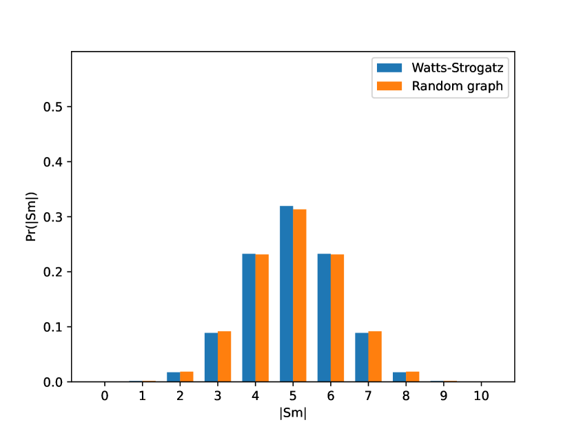
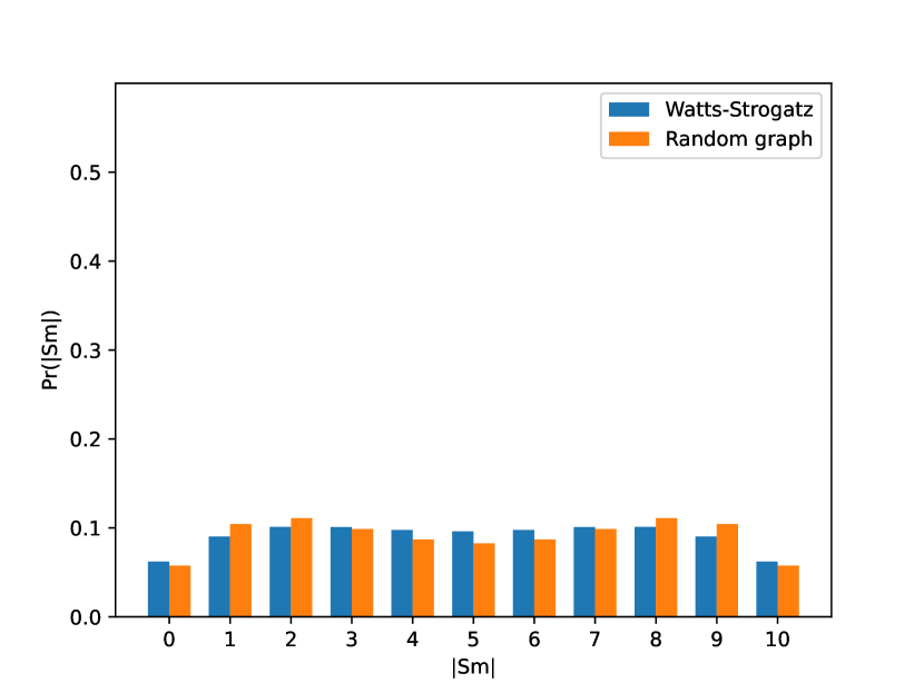
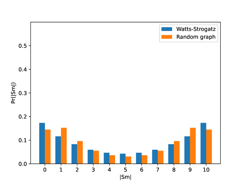
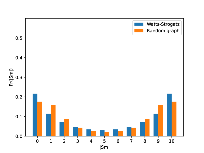
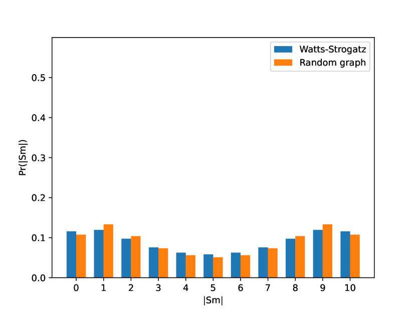
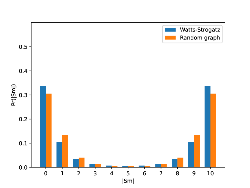
We can use to run exact inference in the MLN described above. We may query the probability that a particular domain member (element) smokes. Obviously, the probability will be the same for any domain member. We will thus combine all of these together and query for the probability of there being exactly smokers, instead.
Denote the theory obtained when we reduce the MLN to . We may answer the query as
To relate our model to others which can be modelled without the linear order axiom, we compare the results to inference over a completely random undirected graph with the same number of edges. Intuitively, completely random graph may form more disconnected components, thus not necessarily preferring the extremes, i.e., either nobody smokes or everybody does. We also keep the parameter relatively small since, for large , even the random graph would likely form just one connected component. The MLN over a random graph is defined as follows:
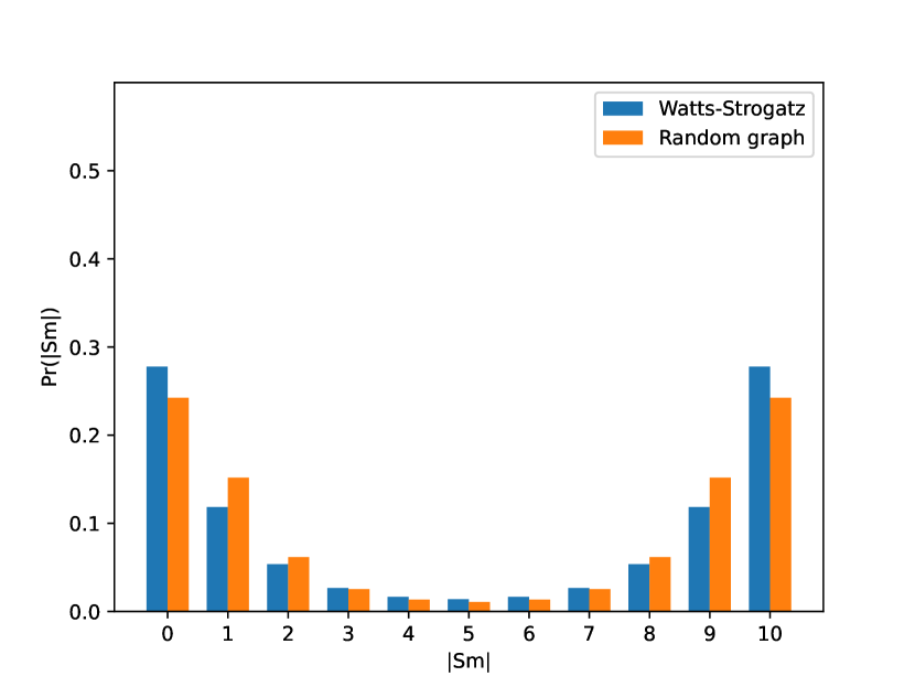
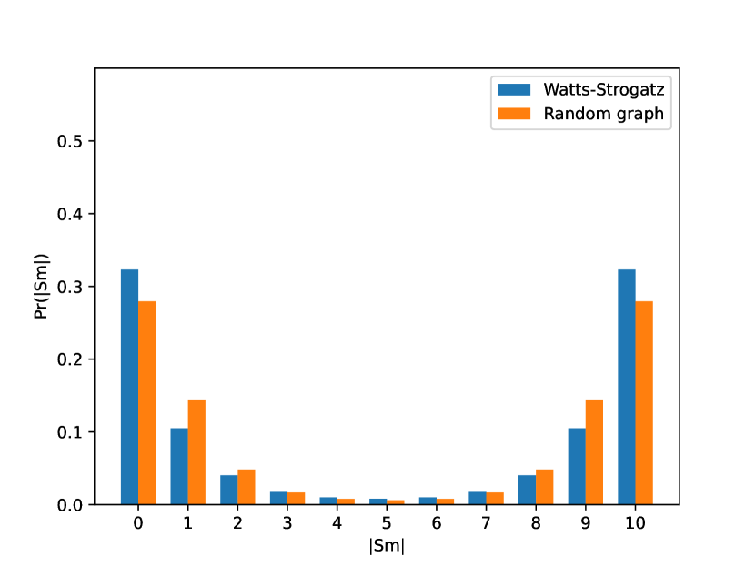
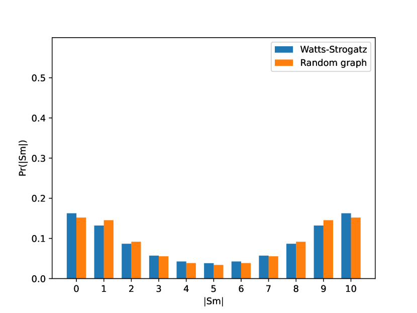
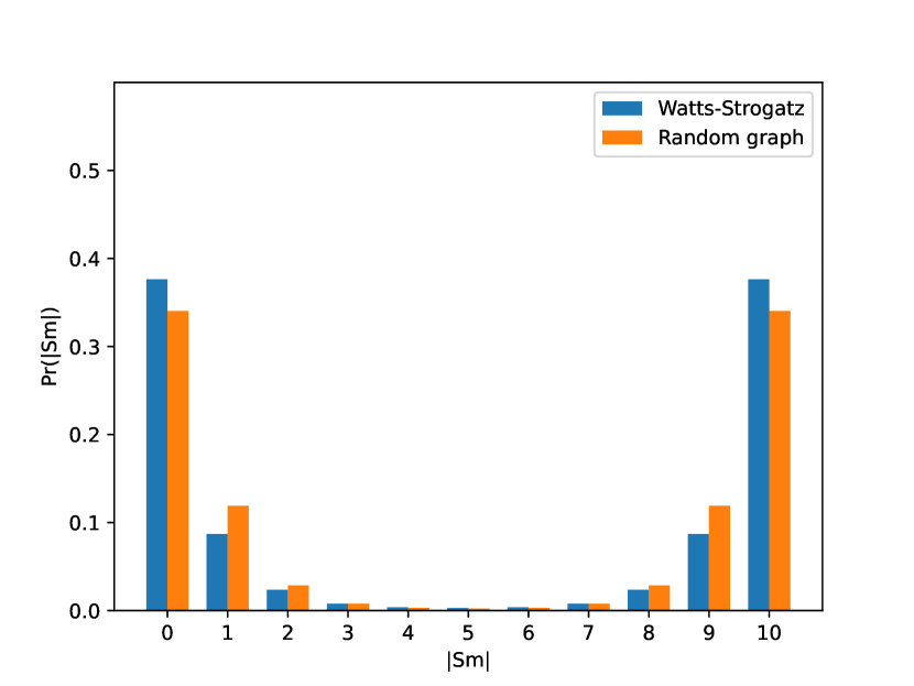
Figures 1, 2 and 3 depict the inference results for a domain size and various weights . The parameter is set to , and , respectively. As one can observe, for smaller , our model approaches the binomial distribution just as the random graph model does. With increasing , the preference for extremes increases as well, and it does so in both models. However, our model clearly prefers the extreme values more, which is consistent with our intuition above.
5 Conclusion
We showed how to compute in with linear order axiom in time polynomial in the domain size. Hence, we showed the language of extended by a linear order to be domain-liftable. The computation can be performed using our new algorithm, .
Acknowledgements
This work was supported by Czech Science Foundation project “Generative Relational Models” (20-19104Y) and partially by the OP VVV project CZ.02.1.01/0.0/0.0/16_019/0000765 “Research Center for Informatics”. JT’s work was also supported by a donation from X-Order Lab.


Appendix A Performance Measurements
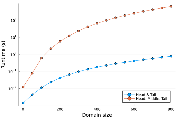
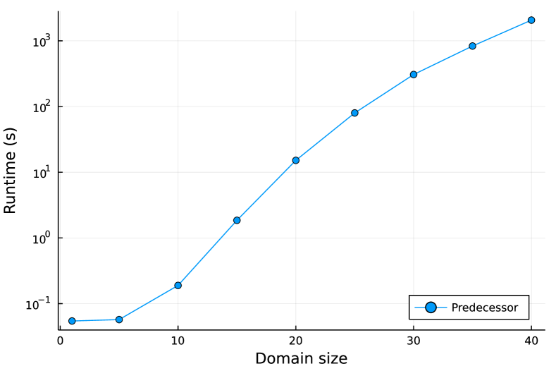
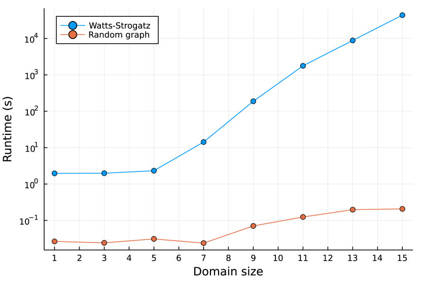
As is already stated above, we implemented in the Julia programming language. Although our implementation is straightforward and without any further optimizations, measuring its execution times still provides us with an intuition about how the algorithm scales to larger domains that are omnipresent in real-world applications. Figure 4 depicts the running times of on a few problems averaged over multiple executions. All experiments were performed in a single thread on a computer with a 64-core AMD EPYC 7742 CPU running at speeds 2.25GHz and 512 GB of RAM.
Figure 4(a) shows execution times for head and tail and head, middle, tail examples. Figure 4(b) depicts the running times on the formula , i.e., only finding the number of possible predecessor relations (of which there are – one for each domain ordering).
Finally, Figure 4(c) depicts execution times of inference on our Watts-Strogatz-like model averaged over various values of . To compute the inference, we resorted to one more implementation trick. Instead of repeatedly computing the probability for each , we turned into a symbolic weight. Thus, we obtained a polynomial in from the computation of . The coefficient for each term of degree then corresponded to the unnormalized probability of . Hence, we were able to compute the entire probability distribution in one call to . The figure depicts running times for those symbolic calls.
References
- Barvínek et al. [2021] Barvínek, J.; van Bremen, T.; Wang, Y.; Železný, F.; and Kuželka, O. 2021. Automatic conjecturing of p-recursions using lifted inference. In Inductive Logic Programming: 30th International Conference, ILP 2021, Virtual Event, October 25–27, 2021, Proceedings, 17–25. Berlin, Heidelberg: Springer-Verlag.
- Beame et al. [2015] Beame, P.; Van den Broeck, G.; Gribkoff, E.; and Suciu, D. 2015. Symmetric weighted first-order model counting. In Proceedings of the 34th ACM SIGMOD-SIGACT-SIGAI Symposium on Principles of Database Systems, PODS ’15, 313–328. New York, NY, USA: Association for Computing Machinery.
- Berge [1971] Berge, C. 1971. Principles of Combinatorics. ISSN. Elsevier Science.
- Bezanson et al. [2017] Bezanson, J.; Edelman, A.; Karpinski, S.; and Shah, V. B. 2017. Julia: A fresh approach to numerical computing. SIAM review 59(1):65–98.
- Charatonik and Witkowski [2015] Charatonik, W., and Witkowski, P. 2015. Two-variable Logic with Counting and a Linear Order. In Kreutzer, S., ed., 24th EACSL Annual Conference on Computer Science Logic (CSL 2015), volume 41 of Leibniz International Proceedings in Informatics (LIPIcs), 631–647. Dagstuhl, Germany: Schloss Dagstuhl–Leibniz-Zentrum fuer Informatik.
- Fieker et al. [2017] Fieker, C.; Hart, W.; Hofmann, T.; and Johansson, F. 2017. Nemo/hecke: Computer algebra and number theory packages for the julia programming language. In Proceedings of the 2017 ACM on International Symposium on Symbolic and Algebraic Computation, ISSAC ’17, 157–164. New York, NY, USA: ACM.
- Getoor and Taskar [2007] Getoor, L., and Taskar, B. 2007. Introduction to statistical relational learning. The MIT Press.
- Grädel, Kolaitis, and Vardi [1997] Grädel, E.; Kolaitis, P. G.; and Vardi, M. Y. 1997. On the decision problem for two-variable first-order logic. Bull. Symb. Log. 3(1):53–69.
- Hinrichs and Genesereth [2006] Hinrichs, T., and Genesereth, M. 2006. Herbrand logic. Technical Report LG-2006-02, Stanford University, Stanford, CA. http://logic.stanford.edu/reports/LG-2006-02.pdf.
- Kazemi et al. [2016] Kazemi, S. M.; Kimmig, A.; Van den Broeck, G.; and Poole, D. 2016. New liftable classes for first-order probabilistic inference. In Proceedings of the 30th International Conference on Neural Information Processing Systems, NIPS’16, 3125–3133. Red Hook, NY, USA: Curran Associates Inc.
- Koller and Friedman [2009] Koller, D., and Friedman, N. 2009. Probabilistic Graphical Models: Principles and Techniques. Adaptive computation and machine learning. MIT Press.
- Kuusisto and Lutz [2018] Kuusisto, A., and Lutz, C. 2018. Weighted model counting beyond two-variable logic. In Proceedings of the 33rd Annual ACM/IEEE Symposium on Logic in Computer Science, LICS 2018, 619–628.
- Kuželka [2021] Kuželka, O. 2021. Weighted first-order model counting in the two-variable fragment with counting quantifiers. Journal of Artificial Intelligence Research 70:1281–1307.
- Libkin [2004] Libkin, L. 2004. Elements of Finite Model Theory. Springer. chapter 1.2, 4.
- Malhotra and Serafini [2022] Malhotra, S., and Serafini, L. 2022. Weighted model counting in with cardinality constraints and counting quantifiers: A closed form formula. In Proceedings of the Thirty-Sixth AAAI Conference on Artificial Intelligence, 5817–5824.
- Richardson and Domingos [2006] Richardson, M., and Domingos, P. 2006. Markov logic networks. Machine Learning 62(1–2):107–136.
- van Bremen and Kuželka [2021a] van Bremen, T., and Kuželka, O. 2021a. Faster lifting for two-variable logic using cell graphs. In de Campos, C., and Maathuis, M. H., eds., Proceedings of the Thirty-Seventh Conference on Uncertainty in Artificial Intelligence, volume 161 of Proceedings of Machine Learning Research, 1393–1402. PMLR.
- van Bremen and Kuželka [2021b] van Bremen, T., and Kuželka, O. 2021b. Lifted Inference with Tree Axioms. In Proceedings of the 18th International Conference on Principles of Knowledge Representation and Reasoning, 599–608.
- Van Den Broeck and Davis [2012] Van Den Broeck, G., and Davis, J. 2012. Conditioning in first-order knowledge compilation and lifted probabilistic inference. In Proceedings of the Twenty-Sixth AAAI Conference on Artificial Intelligence, AAAI’12, 1961–1967. AAAI Press.
- Van den Broeck et al. [2021] Van den Broeck, G.; Kersting, K.; Natarajan, S.; and Poole, D. 2021. An Introduction to Lifted Probabilistic Inference. MIT Press.
- Van den Broeck, Meert, and Darwiche [2014] Van den Broeck, G.; Meert, W.; and Darwiche, A. 2014. Skolemization for weighted first-order model counting. In Proceedings of the Fourteenth International Conference on Principles of Knowledge Representation and Reasoning, KR’14, 111–120. AAAI Press.
- Van den Broeck [2011] Van den Broeck, G. 2011. On the completeness of first-order knowledge compilation for lifted probabilistic inference. In Proceedings of the 24th International Conference on Neural Information Processing Systems, NIPS’11, 1386–1394. Red Hook, NY, USA: Curran Associates Inc.
- Van Haaren et al. [2016] Van Haaren, J.; Van den Broeck, G.; Meert, W.; and Davis, J. 2016. Lifted generative learning of markov logic networks. Machine Learning 103:27–55.
- Wang et al. [2022] Wang, Y.; van Bremen, T.; Wang, Y.; and Kuželka, O. 2022. Domain-lifted sampling for universal two-variable logic and extensions. In Proceedings of the Thirty-Sixth AAAI Conference on Artificial Intelligence, 10070–10079.
- Watts and Strogatz [1998] Watts, D. J., and Strogatz, S. H. 1998. Collective dynamics of ‘small-world’ networks. Nature 393(6684):440–442.
- Zhang, Juba, and Van den Broeck [2021] Zhang, H.; Juba, B.; and Van den Broeck, G. 2021. Probabilistic generating circuits. In International Conference on Machine Learning, 12447–12457. PMLR.