DPM-Solver++: Fast Solver for Guided Sampling of Diffusion Probabilistic Models
Abstract
Diffusion probabilistic models (DPMs) have achieved impressive success in high-resolution image synthesis, especially in recent large-scale text-to-image generation applications. An essential technique for improving the sample quality of DPMs is guided sampling, which usually needs a large guidance scale to obtain the best sample quality. The commonly-used fast sampler for guided sampling is DDIM, a first-order diffusion ODE solver that generally needs 100 to 250 steps for high-quality samples. Although recent works propose dedicated high-order solvers and achieve a further speedup for sampling without guidance, their effectiveness for guided sampling has not been well-tested before. In this work, we demonstrate that previous high-order fast samplers suffer from instability issues, and they even become slower than DDIM when the guidance scale grows large. To further speed up guided sampling, we propose DPM-Solver++, a high-order solver for the guided sampling of DPMs. DPM-Solver++ solves the diffusion ODE with the data prediction model and adopts thresholding methods to keep the solution matches training data distribution. We further propose a multistep variant of DPM-Solver++ to address the instability issue by reducing the effective step size. Experiments show that DPM-Solver++ can generate high-quality samples within only 15 to 20 steps for guided sampling by pixel-space and latent-space DPMs.111Code is available at https://github.com/LuChengTHU/dpm-solver
1 Introduction
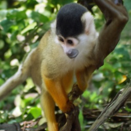
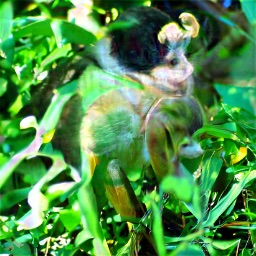
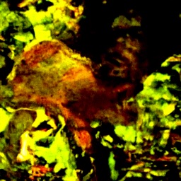
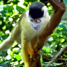
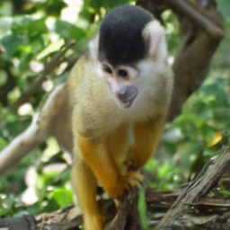
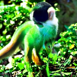
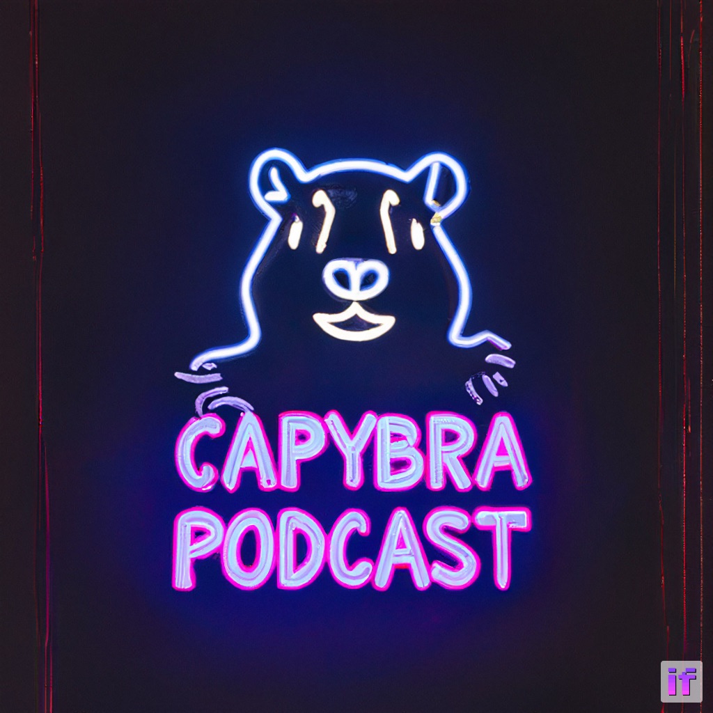
NFE = 10
DPM-Solver++(2M)
(ours)
DDPM
(Ho et al., 2020)

SDE-DPM-Solver++1
(ours)

SDE-DPM-Solver++(2M)
(ours)
NFE = 20
DPM-Solver++(2M)
(ours)
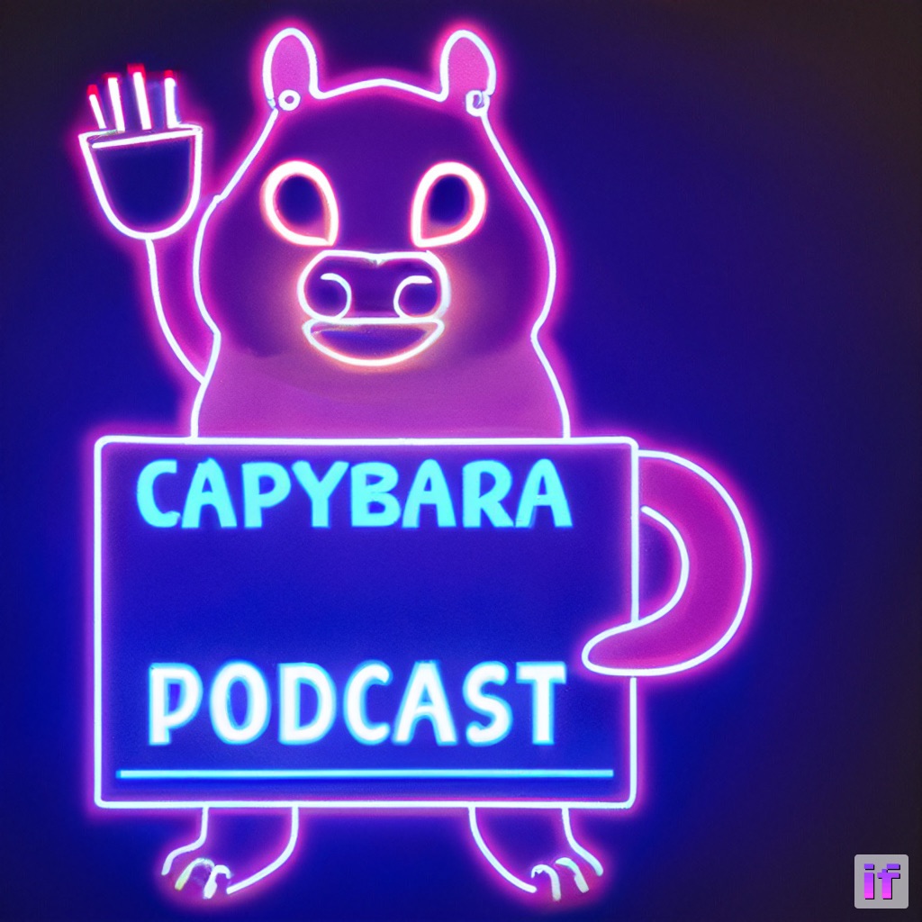
DDPM
(Ho et al., 2020)
SDE-DPM-Solver++1
(ours)
SDE-DPM-Solver++(2M)
(ours)
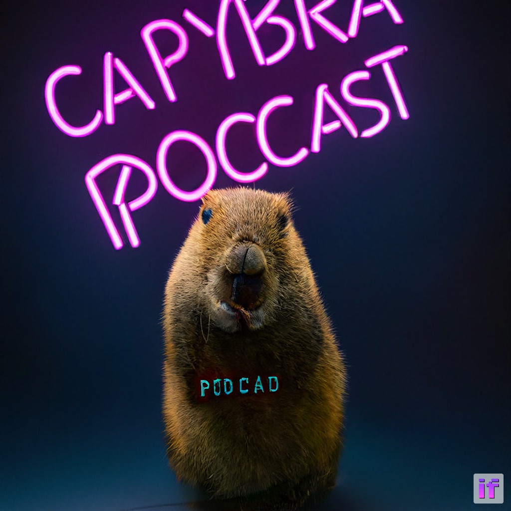
NFE = 50
DPM-Solver++(2M)
(ours)

DDPM
(Ho et al., 2020)
SDE-DPM-Solver++1
(ours)
SDE-DPM-Solver++(2M)
(ours)
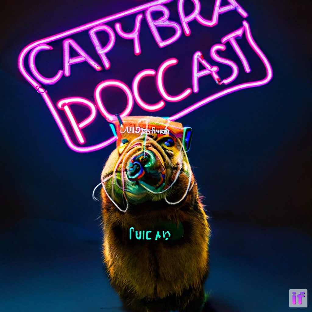
NFE = 100
DPM-Solver++(2M)
(ours)
DDPM
(Ho et al., 2020)
SDE-DPM-Solver++1
(ours)

SDE-DPM-Solver++(2M)
(ours)
Diffusion probabilistic models (DPMs) (Sohl-Dickstein et al., 2015; Ho et al., 2020; Song et al., 2021b) have achieved impressive success on various tasks, such as high-resolution image synthesis (Dhariwal & Nichol, 2021; Ho et al., 2022; Rombach et al., 2022), image editing (Meng et al., 2022; Saharia et al., 2022a; Zhao et al., 2022), text-to-image generation (Nichol et al., 2021; Saharia et al., 2022b; Ramesh et al., 2022; Rombach et al., 2022; Gu et al., 2022), voice synthesis (Liu et al., 2022a; Chen et al., 2021a; b), molecule generation (Xu et al., 2022; Hoogeboom et al., 2022; Wu et al., 2022) and data compression (Theis et al., 2022; Kingma et al., 2021). Compared with other deep generative models such as GANs (Goodfellow et al., 2014) and VAEs (Kingma & Welling, 2014), DPMs can even achieve better sample quality by leveraging an essential technique called guided sampling (Dhariwal & Nichol, 2021; Ho & Salimans, 2021), which uses additional guidance models to improve the sample fidelity and the condition-sample alignment. Through it, DPMs in text-to-image and image-to-image tasks can generate high-resolution photorealistic and artistic images which are highly correlated to the given condition, bringing a new trend in artificial intelligence art painting.
The sampling procedure of DPMs gradually removes the noise from pure Gaussian random variables to obtain clear data, which can be viewed as discretizing either the diffusion SDEs (Ho et al., 2020; Song et al., 2021b) or the diffusion ODEs (Song et al., 2021b; a) defined by a parameterized noise prediction model or data prediction model (Ho et al., 2020; Kingma et al., 2021). Guided sampling of DPMs can also be formalized with such discretizations by combining an unconditional model with a guidance model, where a hyperparameter controls the scale of the guidance model (i.e. guidance scale). The commonly-used method for guided sampling is DDIM (Song et al., 2021a), which is proven as a first-order diffusion ODE solver (Salimans & Ho, 2022; Lu et al., 2022) and it generally needs 100 to 250 steps of large neural network evaluations to converge, which is time-consuming.
Dedicated high-order diffusion ODE solvers (Lu et al., 2022; Zhang & Chen, 2022) can generate high-quality samples in 10 to 20 steps for sampling without guidance. However, their effectiveness for guided sampling has not been carefully examined before. In this work, we demonstrate that previous high-order solvers for DPMs generate unsatisfactory samples for guided sampling, even worse than the simple first-order solver DDIM. We identify two challenges of applying high-order solvers to guided sampling: (1) the large guidance scale narrows the convergence radius of high-order solvers, making them unstable; and (2) the converged solution does not fall into the same range with the original data (a.k.a. “train-test mismatch” (Saharia et al., 2022b)).
Based on the observations, we propose DPM-Solver++, a training-free fast diffusion ODE solver for guided sampling. We find that the parameterization of the DPM critically impacts the solution quality. Subsequently, we solve the diffusion ODE defined by the data prediction model, which predicts the clean data given the noisy ones. We derive a high-order solver for solving the ODE with the data prediction parameterization, and adopt dynamic thresholding methods (Saharia et al., 2022b) to mitigate the train-test mismatch problem. Furthermore, we develop a multistep solver which uses smaller step sizes to address instability.
As shown in Fig. 1, DPM-Solver++ can generate high-quality samples in only 15 steps, which is much faster than all the previous training-free samplers for guided sampling. Our additional experimental results show that DPM-Solver++ can generate high-fidelity samples and almost converge within only 15 to 20 steps, for a wide variety of guided sampling applications, including both pixel-space DPMs and latent-space DPMs.
2 Diffusion Probabilistic Models
In this section, we review diffusion probabilistic models (DPMs) and their sampling methods.
2.1 Fast Sampling for DPMs by Diffusion ODEs
Diffusion Probabilistic Models (DPMs) (Sohl-Dickstein et al., 2015; Ho et al., 2020; Song et al., 2021b) gradually add Gaussian noise to a -dimensional random variable to perturb the corresponding unknown data distribution at time to a simple normal distribution at time for some . The transition distribution at each time satisfies
| (1) |
where and the signal-to-noise-ratio (SNR) is strictly decreasing w.r.t. (Kingma et al., 2021). Eq. (1) can be written as , where .
Parameterization: noise prediction and data prediction
DPMs learn to recover the data based on the noisy input with a sequential denoising procedure. There are two alternative ways to define the model. The noise prediction model attempts to predict the noise from the data , which optimizes the parameter by the following objective (Ho et al., 2020; Song et al., 2021b):
| (2) |
where , , , and is a weighting function. Alternatively, the data prediction model predicts the original data based on the noisy , and its relationship with is given by (Kingma et al., 2021).
Diffusion ODEs
Sampling by DPMs can be implemented by solving the diffusion ODEs (Song et al., 2021b; a; Liu et al., 2022b; Zhang & Chen, 2022; Lu et al., 2022), which is generally faster than other sampling methods. Specifically, sampling by diffusion ODEs need to discretize the following ODE (Song et al., 2021b) with changing from to :
| (3) |
and the equivalent diffusion ODE w.r.t. the data prediction model is
| (4) |
where the coefficients , (Kingma et al., 2021).
2.2 Guided Sampling for DPMs
Guided sampling (Dhariwal & Nichol, 2021; Ho & Salimans, 2021) is a widely-used technique to apply DPMs for conditional sampling, which is useful in text-to-image, image-to-image, and class-to-image applications (Dhariwal & Nichol, 2021; Saharia et al., 2022b; Rombach et al., 2022; Nichol et al., 2021; Ramesh et al., 2022). Given a condition variable , guided sampling defines a conditional noise prediction model . There are two types of guided sampling methods, depending on whether they require a classifier model. Classifier guidance (Dhariwal & Nichol, 2021) leverages a pretrained classifier to define the conditional noise prediction model by:
| (5) |
where is the guidance scale. In practice, a large is usually preferred for improving the condition-sample alignment (Rombach et al., 2022; Saharia et al., 2022b) for guided sampling. Classifier-free guidance (Ho & Salimans, 2021) shares the same parameterized model for the unconditional and conditional noise prediction models, where the input for the unconditional model is a special placeholder . The corresponding conditional model is defined by:
| (6) |
Then, samples can be drawn by solving the ODE (3) with in place of . DDIM (Song et al., 2021a) is a typical solver for guided sampling, which generates samples in a few hundreds of steps.
2.3 Exponential Integrators and High-Order ODE Solvers
It is shown in recent works (Lu et al., 2022; Zhang & Chen, 2022) that ODE solvers based on exponential integrators (Hochbruck & Ostermann, 2010) converge much faster than the traditional solvers for solving the unconditional diffusion ODE (3). Given an initial value at time , Lu et al. (2022) derive the solution of the diffusion ODE (3) at time as:
| (7) |
where the ODE is changed from the time () domain to the log-SNR () domain by the change-of-variables formula. Here, the log-SNR is a strictly decreasing function of with the inverse function , and , are the corresponding change-of-variable forms for . Lu et al. (2022) showed that DDIM is a first-order solver for Eq. (7). They further proposed a high-order solver named “DPM-Solver”, which can generate realistic samples for the unconditional model in only 10-20 steps.
Unfortunately, the outstanding efficiency of existing high-order solvers does not transfer to guided sampling, which we shall discuss soon.
3 Challenges of High-Order Solvers for Guided Sampling
Before developing new fast solvers, we first examine the performance of existing high-order diffusion ODE solvers and highlight the challenges.
The first challenge is the large guidance scale causes high-order solvers to be instable. As shown in Fig. 1, for a large guidance scale and function evaluations, previous high-order diffusion ODE solvers (Lu et al., 2022; Zhang & Chen, 2022; Liu et al., 2022b) produce low-quality images. Their sample quality is even worse than the first-order DDIM. Moreover, the sample quality becomes even worse as the order of the solver gets higher.
Intuitively, large guidance scales may amplify both the output and the derivatives of the model in Eq. (5). The derivatives of the model affect the convergence range of ODE solvers, and the amplification may cause high-order ODE solvers to need much smaller step sizes to converge, and thus the higher-order solvers may perform worse than the first-order solver. Moreover, high-order solvers require high-order derivatives, which are generally more sensitive to the amplifications. This further narrows the convergence radius.
The second challenge is the “train-test mismatch” problem (Saharia et al., 2022b). The data lie in a bounded interval (e.g. for image data). However, the large guidance scale pushes the conditional noise prediction model away from the true noise, which in turns make the sample (i.e. the converged solution of diffusion ODEs) to fall out of the bound. In this case, the generated images are saturated and unnatural (Saharia et al., 2022b).
4 Designing Training-Free Fast Samplers for Guided Sampling
In this section, we design novel high-order diffusion ODE solvers for faster guided sampling. As discussed in Sec. 3, previous high-order solvers have instability and “train-test mismatch” issues for large guidance scales. The “train-test mismatch” issue arises from the ODE itself, and we find the parameterization of the ODE is critical for the converged solution to be bounded. While previous high-order solvers are designed for the noise prediction model , we solve the ODE (4) for the data prediction model , which itself has some advantages and thresholding methods are further available to keep the samples bounded (Ho et al., 2020; Saharia et al., 2022b). We also propose a multistep solver to address the instability issue.
4.1 Designing Solvers by Data Prediction Model
We follow the notations in Lu et al. (2022). Given a sequence decreasing from to and an initial value , the solver aims to iteratively compute a sequence to approximate the exact solution at each time , and the final value is the approximated sample by the diffusion ODE. Denote for .
For solving the diffusion ODE w.r.t. in Eq. (4), we firstly propose a simplified formulation of the exact solution of diffusion ODEs w.r.t. below. Such formulation exactly computes the linear term in Eq. (4) and only remains an exponentially-weighted integral of . Denote as the change-of-variable form of for , we have:
Proposition 4.1 (Exact solution of diffusion ODEs of , proof in Appendix A).
Given an initial value at time , the solution at time of diffusion ODEs in Eq. (4) is:
| (8) |
As the diffusion ODEs in Eq. (3) and Eq.(4) are equivalent, the exact solution formulations in Eq. (7) and Eq. (8) are also equivalent. However, from the prespective of designing ODE solvers, these two formulations are different. Firstly, Eq. (7) exactly computes the linear term , while Eq. (8) exactly computes another the linear term . Moreover, to design ODE solvers, Eq. (7) needs to approximate the integral , while Eq. (8) needs to approximate , and these two integrals are different (recall that ). Therefore, the high-order solvers based on Eq. (7) and Eq. (8) are essentially different. We further propose the general manner for design high-order ODE solvers based on Eq. (8) below.
Given the previous value at time , the aim of our solver is to approximate the exact solution at time . Denote as the -th order total derivatives of w.r.t. logSNR . For , taking the -th Taylor expansion at for w.r.t. and substitute it into Eq. (8) with and , we have
| (9) |
where the integral can be analytically computed by integral-by-parts (detailed in Appendix A). Therefore, to design a -th order ODE solver, we only need to estimate the -th order derivatives for after omitting the high-order error terms, which are well-studied techniques and we discussed in details in Sec. 4.2. A special case is , where the solver is the same as DDIM (Song et al., 2021a), and we discuss in Sec. 6.1.
For , we use a similar technique as DPM-Solver-2 (Lu et al., 2022) to estimate the derivative . Specifically, we introduce an additional intermediate time step between and and combine the function values at and to approximate the derivative, which is the standard manner for singlestep ODE solvers (Atkinson et al., 2011). Overall, we need time steps ( and ) which satisfies . The detailed algorithm is proposed in Algorithm 1, where we combine the previous value at time with the intermediate value at time to compute the value at time .
We name the algorithm as DPM-Solver++(2S), which means that the proposed solver is a second-order singlestep method. We present the theoretical guarantee of the convergence order in Appendix A. For , as discussed in Sec. 3, high-order solvers may be unsuitable for large guidance scales, thus we mainly consider in this work, and leave the solvers for higher orders for future study.
4.2 From Singlestep to Multistep
At each step (from to ), the proposed singlestep solver needs two sequential function evaluations of the neural network . Moreover, the intermediate values are only used once and then discarded. Such method loses the previous information and may be inefficient. In this section, we propose another second-order diffusion ODE solver which uses the previous information at each step.
In general, to approximate the derivatives in Eq. (9) for , there is another mainstream approach (Atkinson et al., 2011): multistep methods (such as Adams–Bashforth methods). Given the previous values at time , multistep methods just reuse the previous values to approximate the high-order derivatives. Multistep methods are empirically more efficient than singlestep methods, especially for limited number of function evaluations. (Atkinson et al., 2011)
We combine the techniques for designing multistep solvers with the Taylor expansions in Eq. (9) and further propose a multistep second-order solver for diffusion ODEs with . The detailed algorithm is proposed in Algorithm 2, where we combine the previous values and to compute the value without additional intermediate values. We name the algorithm as DPM-Solver++(2M), which means that the proposed solver is a second-order multistep solver. We also present a detailed theoretical guarantee of the convergence order, which is stated in Appendix A.
For a fixed budget of the total number of function evaluations, multistep methods can use steps, while -th order singlestep methods can only use no more than steps. Therefore, each step size of multistep methods is around of that of singlestep methods, so the high-order error terms in Eq. (9) of multistep methods may also be smaller than those of singlestep methods. We show in Sec. 7.1 that the multistep methods are slightly better than singlestep methods.
4.3 Combining Thresholding with DPM-Solver++
For distributions of bounded data (such as the image data), thresholding methods (Ho et al., 2020; Saharia et al., 2022b) can push out-of-bound samples inwards and somehow reduce the adverse impact of the large guidance scale. Specifically, thresholding methods define a clipped data prediction model by elementwise clipping the original model within the data bound, which results in better sample quality for large guidance scales (Saharia et al., 2022b). As our proposed DPM-Solver++ is designed for the model, we can straightforwardly combine thresholding methods with DPM-Solver++.
5 Fast Solvers for Diffusion SDEs
Sampling by diffusion models can be alternatively implemented by solving Diffusion SDEs (Song et al., 2021b):
| (10) |
where is the reverse-time Wiener process from to . In this section, we consider the diffusion SDEs w.r.t. log-SNR , and derive the corresponding second-order solvers.
Denote as the corresponding Wiener process w.r.t. . For simplicity, we denote , , , . For VP-type diffusion models (Song et al., 2021b) (i.e. ), we have and . As and (Kingma et al., 2021). the diffusion SDEs w.r.t. is
| (11) | ||||
| (12) |
By applying variation-of-constants formula, we propose the exact solution of diffusion SDEs as following.
Proposition 5.1 (Exact solution of diffusion SDEs, proof in Appendix A).
Given an initial value at time , the solution at time of diffusion SDEs in Eq. (10) is:
| (13) | ||||
| (14) |
Moreover, we can compute the Itô-integral by
| (15) | ||||
| (16) |
where . Thus, we can discretize the integral w.r.t. or to get the corresponding solvers for diffusion SDEs, which is presented below. For simplicity, we denote that .
SDE-DPM-Solver-1
Let . By assuming , we have
| (17) |
SDE-DPM-Solver++1
Let . By assuming , we have
| (18) |
SDE-DPM-Solver-2M
Let . Assume we have a previous solution with its model output at time . Denote . By assuming , we have
| (19) |
SDE-DPM-Solver++(2M)
Let . Assume we have a previous solution with its model output at time . Denote . By assuming , we have
| (20) |
6 Relationship with Other Fast Sampling Methods
In essence, all training-free sampling methods for DPMs can be understood as either discretizing diffusion SDEs (Ho et al., 2020; Song et al., 2021b; Jolicoeur-Martineau et al., 2021; Tachibana et al., 2021; Kong & Ping, 2021; Bao et al., 2022b; Zhang et al., 2022) or discretizing diffusion ODEs (Song et al., 2021b; a; Liu et al., 2022b; Zhang & Chen, 2022; Lu et al., 2022). As DPM-Solver++ is designed for solving diffusion ODEs, in this section, we discuss the relationship between DPM-Solver++ and other diffusion ODE solvers. We further briefly discuss other fast sampling methods for DPMs.
6.1 Comparison with Solvers based on Exponential Integrators
The general version of DDIM with is (Song et al., 2021a)
| (21) |
Previous state-of-the-art fast diffusion ODE solvers (Lu et al., 2022; Zhang & Chen, 2022) leverages exponential integrators to solve diffusion ODEs with noise prediction models . In short, these solvers approximate the exact solution in Eq. (7) and include DDIM (Song et al., 2021a) with as the first-order case. Below we show that the first-order case for DPM-Solver++ is also DDIM.
For , Eq. (9) becomes (after omitting the terms)
Therefore, our proposed DPM-Solver++ is the high-order generalization of DDIM () w.r.t. the data prediction model . To the best of our knowledge, such generalization has not been proposed before. We list the detailed difference between previous high-order solvers based on exponential integrators and DPM-Solver++ in Table 1. We emphasize that although the first-order version of these solvers are equivalent, the high-order versions of these solvers are rather different.
In addition, for DDIM with , it is easy to verify that such a stochastic DDIM is equivalent to SDE-DPM-Solver++1. Therefore, our proposed SDE-DPM-Solver++(2M) is a second-order generalized version of the first-order stochastic DDIM. To the best of our knowledge, such a finding is not revealed in previous works.
6.2 Other Fast Sampling Methods
Samplers based on diffusion SDEs (Ho et al., 2020; Song et al., 2021b; Jolicoeur-Martineau et al., 2021; Tachibana et al., 2021; Kong & Ping, 2021; Bao et al., 2022b; Zhang et al., 2022) generally needs more steps to converge than those based on diffusion ODEs (Lu et al., 2022), because SDEs introduce more randomness and make denoising more difficult. Samplers based on extra training include model distillation (Salimans & Ho, 2022; Luhman & Luhman, 2021), learning reverse process variances (San-Roman et al., 2021; Nichol & Dhariwal, 2021; Bao et al., 2022a), and learning sampling steps (Lam et al., 2021; Watson et al., 2022). However, training-based samplers are hard to scale-up to pre-trained large DPMs (Saharia et al., 2022b; Rombach et al., 2022; Ramesh et al., 2022). There are other fast sampling methods by modifying the original DPMs to a latent space (Vahdat et al., 2021) or with momentum (Dockhorn et al., 2022). In addition, combining DPMs with GANs (Xiao et al., 2022; Wang et al., 2022) improves the sample quality of GANs and sampling speed of DPMs.
7 Experiments
In this section, we show that DPM-Solver++ can speed up both the pixel-space DPMs and the latent-space DPMs for guided sampling. We vary different number of function evaluations (NFE) which is the numebr of calls to the model or , and compare DPM-Solver++ with the previous state-of-the-art fast samplers for DPMs including DPM-Solver (Lu et al., 2022), DEIS (Zhang & Chen, 2022), PNDM (Liu et al., 2022b) and DDIM (Song et al., 2021a). We also convert the discrete-time DPMs to the continuous-time and use these continuous-time solvers. We refer to Appendix C for the detailed implementations and experiment settings.
As previous solvers did not test the performance in guided sampling, we also carefully tune the baseline samplers by ablating the step size schedule (i.e. the choice for the time steps ) and the solver order. We find that
-
•
For the step size schedule, we search the time steps in the following choices: uniform (a widely-used setting in high-resolution image synthesis), uniform (used in (Lu et al., 2022)), uniform split of the power functions of (used in (Zhang & Chen, 2022), detailed in Appendix C), and we find that the best choice is uniform . Thus, we use uniform for the time steps in all of our experiments for all of the solvers.
-
•
We find that for a large guidance scale, the best choice for all the previous solvers is the second-order (i.e. DPM-Solver-2 and DEIS-1). However, for a comprehensive comparison, we run all the orders of previous solvers, including DPM-Solver-2 and DPM-Solver-3; DEIS-1, DEIS-2 and DEIS-3 and choose their best result for each NFE in our comparison.
We run both DPM-Solver++(2S) and DPM-Solver++(2M), and we find that for large guidance scales, the multistep DPM-Solver++(2M) performs better; and for a slightly small guidance scales, the singlestep DPM-Solver++(2S) performs better. We report the best results of DPM-Solver++ and all of the previous samplers in the following sections, the detailed values are listed in Appendix D.
7.1 Pixel-Space DPMs with Guidance
(a) Pixel-space DPM
()
(b) Pixel-space DPM
()
(c) Pixel-space DPM
()
(d) Latent-space DPM
()
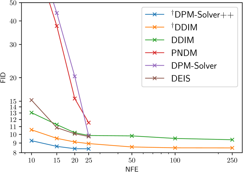
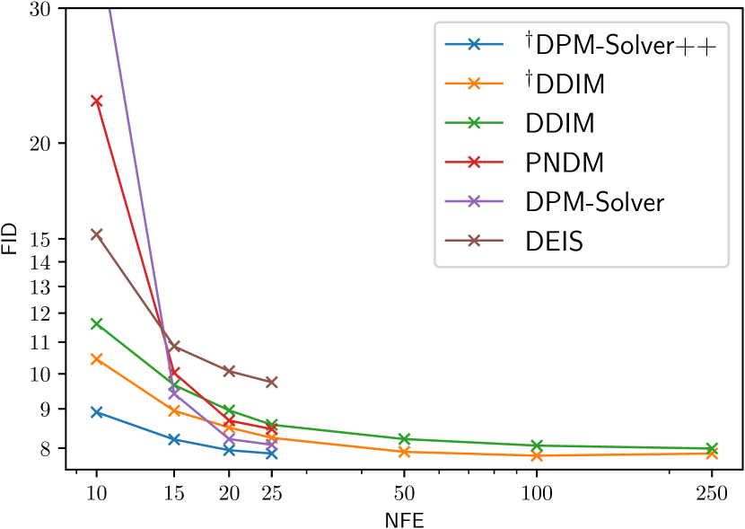
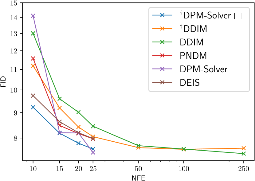
We firstly compare DPM-Solver++ with other samplers for the guided sampling with classifier-guidance on ImageNet 256x256 dataset by the pretrained DPMs(Dhariwal & Nichol, 2021). We measure the sample quality by drawing 10K samples and computing the widely-used FID score (Heusel et al., 2017), where lower FID usually implies better sample quality. We also adopt the dynamic thresholding method (Saharia et al., 2022b) for both DDIM and DPM-Solver++. We vary the guidance scale in 8.0, 4.0 and 2.0, the results are shown in Fig. 4(a-c). We find that for large guidance scales, all the previous high-order samplers (DEIS, PNDM, DPM-Solver) converge slower than the first-order DDIM, which shows that previous high-order samplers are unstable. Instead, DPM-Solver++ achieve the best speedup performance for both large guidance scales and small guidance scales. Especially for large guidance scales, DPM-Solver++ can almost converge within only NFE.
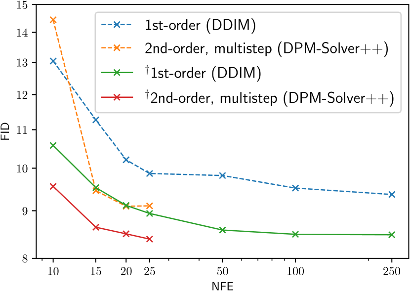
As an ablation, we also compare the singlestep DPM-Solver-2, the singlestep DPM-Solver++(2S) and the multistep DPM-Solver++(2M) to demonstrate the effectiveness of our method. We use a large guidance scale and conduct the following ablations:
-
•
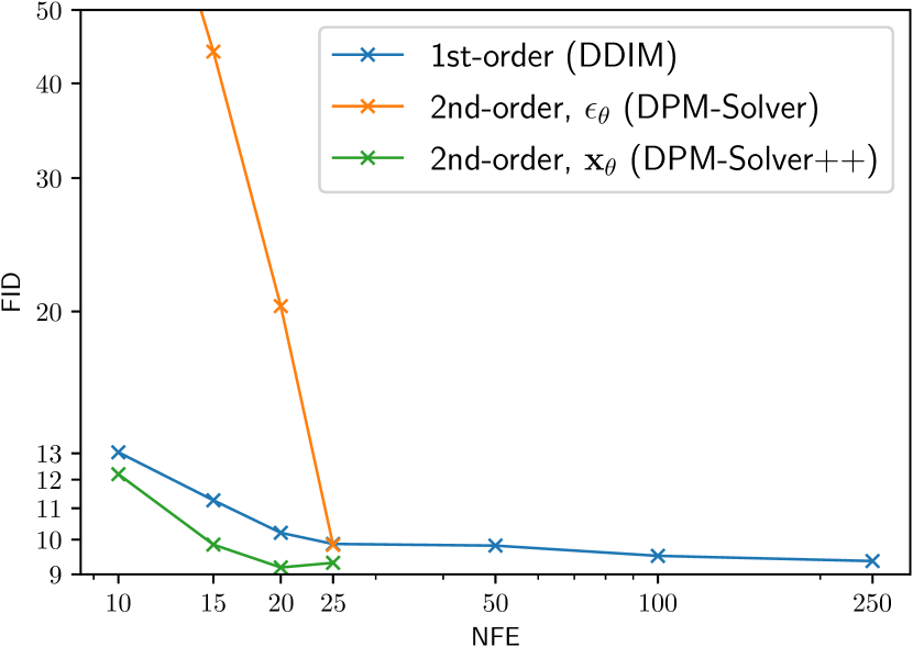
From to : As shown in Fig. 3(a), by simply changing the solver from to (i.e. from DPM-Solver-2 to DPM-Solver++(2S)), the solver can achieve a stable acceleration performance which is faster than the first-order DDIM. Such result indicates that for guided sampling, high-order solvers w.r.t. may be more preferred than those w.r.t. .
-
•
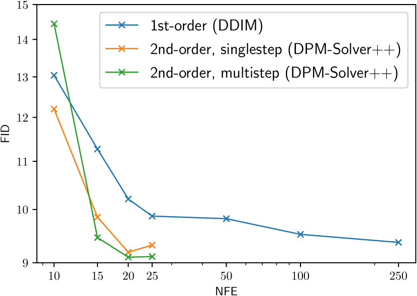
From singlestep to multistep: As show in Fig. 3(b), the multistep DPM-Solver++(2M) converges slightly faster than the singlestep DPM-Solver++(2S), which almost converges in 15 NFE. Such result indicates that for guided sampling with a large guidance scale, multistep methods may be faster than singlestep methods.
-
•
With or without thresholding: We compare the performance of DDIM and DPM-Solver++ with / without thresholding methods in Fig. 3(c). Note that the thresholding method changes the model and thus also changes the converged solutions of diffusion ODEs. Firstly, we find that after using the thresholding method, the diffusion ODE can generate higher quality samples, which is consistent with the conclusion in (Saharia et al., 2022b). Secondly, the sample quality of DPM-Solver++ with thresholding outperforms DPM-Solver++ without thresholding under the same NFE. Moreover, when combined with thresholding, DPM-Solver++ is faster than the first-order DDIM, which shows that DPM-Solver++ can also speed up guided sampling by DPMs with thresholding methods.
7.2 Latent-Space DPMs with Guidance
We also evaluate DPM-Solver++ on the latent-space DPMs (Rombach et al., 2022), which is recently popular among the community due to their official code “stable-diffusion”. We use the default guidance scale in their official code. The latent-space DPMs map the image data with a latent code by training a pair of encoder and decoder, and then train a DPM for the latent code. As the latent code is unbounded, we do not apply the thresholding method.
Specifically, we randomly sample 10K caption-image pairs from the MS-COCO2014 validation dataset and use the captions as conditions to draw 10K images from the pretrained “stable-diffusion” model, and we only draw a single image sample of each caption, following the standard evaluation procedures in (Nichol et al., 2021; Rombach et al., 2022). We find that all the solvers can achieve a FID around 15.0 to 16.0 even within only 10 steps, which is very close to the FID computed by the converged samples reported in the official page of “stable-diffusion”. We believe it is due to the powerful pretrained decoder, which can map a non-converged latent code to a good image sample.
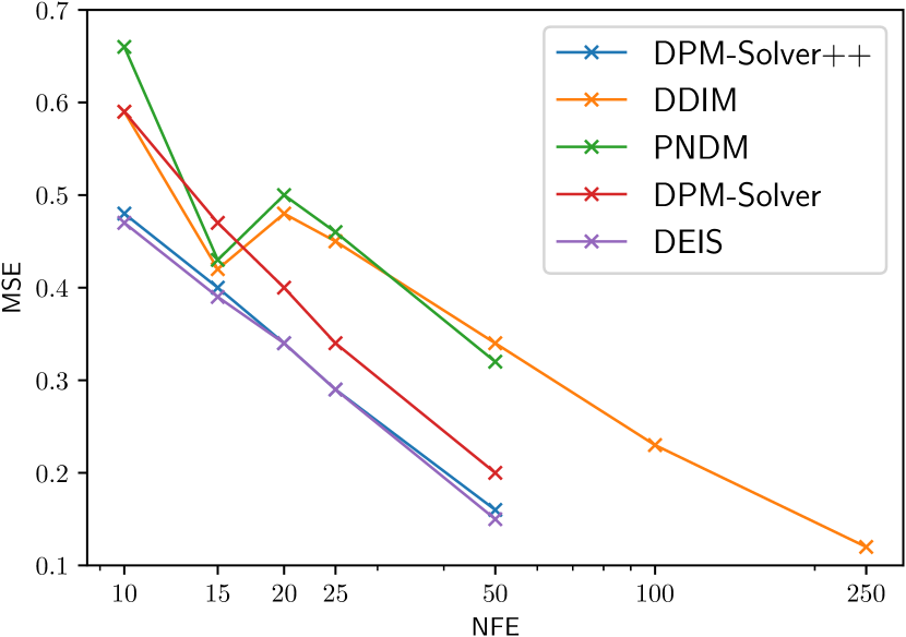
For latent-space DPMs, different diffusion ODE solvers directly affect the convergence speed on the latent space. To further compare different samplers for latent-space DPMs, we directly compare different solvers according to the convergence error on the latent space by the L2-norm between the sampled and the true solution (and the error between them is ). Specifically, we firstly sample 10K noise variables from the standard normal distribution and fix them. Then we sample 10K latent codes by different DPM samplers, starting from the 10K fixed noise variables. As all these solvers can be understood as discretizing diffusion ODEs, we compare the sampled latent codes by the true solution from a 999-step DDIM with samples by different samplers within different NFE, and the results are shown in Fig. 4(d). We find that the supported fast samplers (DDIM and PNDM) in “stable-diffusion” converge much slower than DPM-Solver++ and DEIS, and we find that the second-order multistep DPM-Solver++ and DEIS achieve a quite close speedup on the latent space. Moreover, as “stable-diffusion” by default use PNDM with 50 steps, we find that DPM-Solver++ can achieve a similar convergence error with only 15 to 20 steps. We also present an empirical comparison of the sampled images between different solvers in Appendix D, and we find that DPM-Solver++ can indeed generate quite good image samples within only 15 to 20 steps.
8 Conclusions
We study the problem of accelerating guided sampling of DPMs. We demonstrate that previous high-order solvers based on the noise prediction models are abnormally unstable and generate worse-quality samples than the first-order solver DDIM for guided sampling with large guidance scales. To address this issue and speed up guided sampling, we propose DPM-Solver++, a training-free fast diffusion ODE solver for guided sampling. DPM-Solver++ is based on the diffusion ODE with the data prediction models, which can directly adopt the thresholding methods to stabilize the sampling procedure further. We propose both singlestep and multistep variants of DPM-Solver++. Experiment results show that DPM-Solver++ can generate high-fidelity samples and almost converge within only 15 to 20 steps, applicable for pixel-space and latent-space DPMs.
Ethics Statement
Like other deep generative models such as GANs, DPMs may also be used to generate adverse fake contents (images). The proposed solver can accelerate the guided sampling by DPMs which can further be used for image editing and generate photorealistic fake images. Such influence may further amplify the potential undesirable affects of DPMs for malicious applications.
Reproducibility Statement
Our code is based on the official code of DPM-Solver (Lu et al., 2022) and the pretrained checkpoints in Dhariwal & Nichol (2021) and Stable-Diffusion (Rombach et al., 2022). We will release it after the blind review. In addition, datasets used in experiments are publicly available. Our detailed experiment settings and implementations are listed in Appendix C, and the proof of the solver convergence guarantee are presented in Appendix A.
References
- Atkinson et al. (2011) Kendall Atkinson, Weimin Han, and David E Stewart. Numerical solution of ordinary differential equations, volume 108. John Wiley & Sons, 2011.
- Bao et al. (2022a) Fan Bao, Chongxuan Li, Jiacheng Sun, Jun Zhu, and Bo Zhang. Estimating the optimal covariance with imperfect mean in diffusion probabilistic models. arXiv preprint arXiv:2206.07309, 2022a.
- Bao et al. (2022b) Fan Bao, Chongxuan Li, Jun Zhu, and Bo Zhang. Analytic-DPM: An analytic estimate of the optimal reverse variance in diffusion probabilistic models. In International Conference on Learning Representations, 2022b.
- Chen et al. (2021a) Nanxin Chen, Yu Zhang, Heiga Zen, Ron J. Weiss, Mohammad Norouzi, and William Chan. Wavegrad: Estimating gradients for waveform generation. In International Conference on Learning Representations, 2021a.
- Chen et al. (2021b) Nanxin Chen, Yu Zhang, Heiga Zen, Ron J. Weiss, Mohammad Norouzi, Najim Dehak, and William Chan. Wavegrad 2: Iterative refinement for text-to-speech synthesis. In International Speech Communication Association, pp. 3765–3769, 2021b.
- DeepFloyd (2023) DeepFloyd. If. https://github.com/deep-floyd/IF, 2023.
- Dhariwal & Nichol (2021) Prafulla Dhariwal and Alexander Quinn Nichol. Diffusion models beat GANs on image synthesis. In Advances in Neural Information Processing Systems, volume 34, pp. 8780–8794, 2021.
- Dockhorn et al. (2022) Tim Dockhorn, Arash Vahdat, and Karsten Kreis. Score-based generative modeling with critically-damped Langevin diffusion. In International Conference on Learning Representations, 2022.
- Goodfellow et al. (2014) Ian J. Goodfellow, Jean Pouget-Abadie, Mehdi Mirza, Bing Xu, David Warde-Farley, Sherjil Ozair, Aaron C. Courville, and Yoshua Bengio. Generative adversarial nets. In Advances in Neural Information Processing Systems, volume 27, pp. 2672–2680, 2014.
- Gu et al. (2022) Shuyang Gu, Dong Chen, Jianmin Bao, Fang Wen, Bo Zhang, Dongdong Chen, Lu Yuan, and Baining Guo. Vector quantized diffusion model for text-to-image synthesis. In Proceedings of the IEEE/CVF Conference on Computer Vision and Pattern Recognition, pp. 10696–10706, 2022.
- Heusel et al. (2017) Martin Heusel, Hubert Ramsauer, Thomas Unterthiner, Bernhard Nessler, and Sepp Hochreiter. GANs trained by a two time-scale update rule converge to a local Nash equilibrium. In Isabelle Guyon, Ulrike von Luxburg, Samy Bengio, Hanna M. Wallach, Rob Fergus, S. V. N. Vishwanathan, and Roman Garnett (eds.), Advances in Neural Information Processing Systems, volume 30, pp. 6626–6637, 2017.
- Ho & Salimans (2021) Jonathan Ho and Tim Salimans. Classifier-free diffusion guidance. In NeurIPS 2021 Workshop on Deep Generative Models and Downstream Applications, 2021.
- Ho et al. (2020) Jonathan Ho, Ajay Jain, and Pieter Abbeel. Denoising diffusion probabilistic models. In Advances in Neural Information Processing Systems, volume 33, pp. 6840–6851, 2020.
- Ho et al. (2022) Jonathan Ho, Chitwan Saharia, William Chan, David J Fleet, Mohammad Norouzi, and Tim Salimans. Cascaded diffusion models for high fidelity image generation. Journal of Machine Learning Research, 23(47):1–33, 2022.
- Hochbruck & Ostermann (2010) Marlis Hochbruck and Alexander Ostermann. Exponential integrators. Acta Numerica, 19:209–286, 2010.
- Hoogeboom et al. (2022) Emiel Hoogeboom, Victor Garcia Satorras, Clément Vignac, and Max Welling. Equivariant diffusion for molecule generation in 3D. In International Conference on Machine Learning, pp. 8867–8887. PMLR, 2022.
- Jolicoeur-Martineau et al. (2021) Alexia Jolicoeur-Martineau, Ke Li, Rémi Piché-Taillefer, Tal Kachman, and Ioannis Mitliagkas. Gotta go fast when generating data with score-based models. arXiv preprint arXiv:2105.14080, 2021.
- Kingma & Welling (2014) Diederik P. Kingma and Max Welling. Auto-encoding variational bayes. In International Conference on Learning Representations, 2014.
- Kingma et al. (2021) Diederik P Kingma, Tim Salimans, Ben Poole, and Jonathan Ho. Variational diffusion models. In Advances in Neural Information Processing Systems, 2021.
- Kong & Ping (2021) Zhifeng Kong and Wei Ping. On fast sampling of diffusion probabilistic models. arXiv preprint arXiv:2106.00132, 2021.
- Lam et al. (2021) Max WY Lam, Jun Wang, Rongjie Huang, Dan Su, and Dong Yu. Bilateral denoising diffusion models. arXiv preprint arXiv:2108.11514, 2021.
- Liu et al. (2022a) Jinglin Liu, Chengxi Li, Yi Ren, Feiyang Chen, and Zhou Zhao. Diffsinger: Singing voice synthesis via shallow diffusion mechanism. In Proceedings of the AAAI Conference on Artificial Intelligence, volume 36, pp. 11020–11028, 2022a.
- Liu et al. (2022b) Luping Liu, Yi Ren, Zhijie Lin, and Zhou Zhao. Pseudo numerical methods for diffusion models on manifolds. arXiv preprint arXiv:2202.09778, 2022b.
- Lu et al. (2022) Cheng Lu, Yuhao Zhou, Fan Bao, Jianfei Chen, Chongxuan Li, and Jun Zhu. Dpm-solver: A fast ode solver for diffusion probabilistic model sampling in around 10 steps. arXiv preprint arXiv:2206.00927, 2022.
- Luhman & Luhman (2021) Eric Luhman and Troy Luhman. Knowledge distillation in iterative generative models for improved sampling speed. arXiv preprint arXiv:2101.02388, 2021.
- Meng et al. (2022) Chenlin Meng, Yang Song, Jiaming Song, Jiajun Wu, Jun-Yan Zhu, and Stefano Ermon. SDEdit: Image synthesis and editing with stochastic differential equations. In International Conference on Learning Representations, 2022.
- Nichol et al. (2021) Alex Nichol, Prafulla Dhariwal, Aditya Ramesh, Pranav Shyam, Pamela Mishkin, Bob McGrew, Ilya Sutskever, and Mark Chen. Glide: Towards photorealistic image generation and editing with text-guided diffusion models. arXiv preprint arXiv:2112.10741, 2021.
- Nichol & Dhariwal (2021) Alexander Quinn Nichol and Prafulla Dhariwal. Improved denoising diffusion probabilistic models. In International Conference on Machine Learning, pp. 8162–8171. PMLR, 2021.
- Ramesh et al. (2022) Aditya Ramesh, Prafulla Dhariwal, Alex Nichol, Casey Chu, and Mark Chen. Hierarchical text-conditional image generation with CLIP latents. arXiv preprint arXiv:2204.06125, 2022.
- Rombach et al. (2022) Robin Rombach, Andreas Blattmann, Dominik Lorenz, Patrick Esser, and Björn Ommer. High-resolution image synthesis with latent diffusion models. In Proceedings of the IEEE/CVF Conference on Computer Vision and Pattern Recognition, pp. 10684–10695, 2022.
- Saharia et al. (2022a) Chitwan Saharia, William Chan, Huiwen Chang, Chris Lee, Jonathan Ho, Tim Salimans, David Fleet, and Mohammad Norouzi. Palette: Image-to-image diffusion models. In ACM SIGGRAPH 2022 Conference Proceedings, pp. 1–10, 2022a.
- Saharia et al. (2022b) Chitwan Saharia, William Chan, Saurabh Saxena, Lala Li, Jay Whang, Emily Denton, Seyed Kamyar Seyed Ghasemipour, Burcu Karagol Ayan, S Sara Mahdavi, Rapha Gontijo Lopes, et al. Photorealistic text-to-image diffusion models with deep language understanding. arXiv preprint arXiv:2205.11487, 2022b.
- Salimans & Ho (2022) Tim Salimans and Jonathan Ho. Progressive distillation for fast sampling of diffusion models. In International Conference on Learning Representations, 2022.
- San-Roman et al. (2021) Robin San-Roman, Eliya Nachmani, and Lior Wolf. Noise estimation for generative diffusion models. arXiv preprint arXiv:2104.02600, 2021.
- Sohl-Dickstein et al. (2015) Jascha Sohl-Dickstein, Eric Weiss, Niru Maheswaranathan, and Surya Ganguli. Deep unsupervised learning using nonequilibrium thermodynamics. In International Conference on Machine Learning, pp. 2256–2265. PMLR, 2015.
- Song et al. (2021a) Jiaming Song, Chenlin Meng, and Stefano Ermon. Denoising diffusion implicit models. In International Conference on Learning Representations, 2021a.
- Song et al. (2021b) Yang Song, Jascha Sohl-Dickstein, Diederik P. Kingma, Abhishek Kumar, Stefano Ermon, and Ben Poole. Score-based generative modeling through stochastic differential equations. In International Conference on Learning Representations, 2021b.
- Tachibana et al. (2021) Hideyuki Tachibana, Mocho Go, Muneyoshi Inahara, Yotaro Katayama, and Yotaro Watanabe. Itô-Taylor sampling scheme for denoising diffusion probabilistic models using ideal derivatives. arXiv preprint arXiv:2112.13339, 2021.
- Theis et al. (2022) Lucas Theis, Tim Salimans, Matthew D Hoffman, and Fabian Mentzer. Lossy compression with gaussian diffusion. arXiv preprint arXiv:2206.08889, 2022.
- Vahdat et al. (2021) Arash Vahdat, Karsten Kreis, and Jan Kautz. Score-based generative modeling in latent space. In Advances in Neural Information Processing Systems, volume 34, pp. 11287–11302, 2021.
- Wang et al. (2022) Zhendong Wang, Huangjie Zheng, Pengcheng He, Weizhu Chen, and Mingyuan Zhou. Diffusion-gan: Training gans with diffusion. arXiv preprint arXiv:2206.02262, 2022.
- Watson et al. (2022) Daniel Watson, William Chan, Jonathan Ho, and Mohammad Norouzi. Learning fast samplers for diffusion models by differentiating through sample quality. In International Conference on Learning Representations, 2022.
- Wu et al. (2022) Lemeng Wu, Chengyue Gong, Xingchao Liu, Mao Ye, and Qiang Liu. Diffusion-based molecule generation with informative prior bridges. arXiv preprint arXiv:2209.00865, 2022.
- Xiao et al. (2022) Zhisheng Xiao, Karsten Kreis, and Arash Vahdat. Tackling the generative learning trilemma with denoising diffusion GANs. In International Conference on Learning Representations, 2022.
- Xu et al. (2022) Minkai Xu, Lantao Yu, Yang Song, Chence Shi, Stefano Ermon, and Jian Tang. Geodiff: A geometric diffusion model for molecular conformation generation. arXiv preprint arXiv:2203.02923, 2022.
- Zhang & Chen (2022) Qinsheng Zhang and Yongxin Chen. Fast sampling of diffusion models with exponential integrator. arXiv preprint arXiv:2204.13902, 2022.
- Zhang et al. (2022) Qinsheng Zhang, Molei Tao, and Yongxin Chen. gddim: Generalized denoising diffusion implicit models. arXiv preprint arXiv:2206.05564, 2022.
- Zhao et al. (2022) Min Zhao, Fan Bao, Chongxuan Li, and Jun Zhu. Egsde: Unpaired image-to-image translation via energy-guided stochastic differential equations. arXiv preprint arXiv:2207.06635, 2022.
Appendix A Additional Proofs
A.1 Proof of Proposition 4.1
Taking derivative w.r.t. in Eq. (8) yields
where the last inequality follows from the definitions , .
A.2 Proof of Proposition 5.1
Proof.
For diffusion SDEs w.r.t. the noise prediction model , we have
| (22) | ||||
| (23) | ||||
| (24) |
And for diffusion SDEs w.r.t. the data prediction model , we have
| (25) | ||||
| (26) | ||||
| (27) |
∎
A.3 Derivation of SDE Solvers
SDE-DPM-Solver-1
We have
| (28) | ||||
| (29) |
SDE-DPM-Solver++1
We have
| (30) | ||||
| (31) |
SDE-DPM-Solver-2M
We have
| (32) | |||
| (33) | |||
| (34) |
We can also applying the same approximation as in Lu et al. (2022) by
| (35) |
thus we have
| (36) | |||
| (37) |
SDE-DPM-Solver++2M
We have
| (38) | |||
| (39) | |||
| (40) |
We can also applying the same approximation as in Lu et al. (2022) by
| (41) |
thus we have
| (42) | |||
| (43) |
A.4 Convergence of Algorithms
We make the following assumptions as in Lu et al. (2022) for , i.e.,
-
•
, and exist and are continuous (and hence are bounded).
-
•
The map is -Lipschitz.
-
•
.
We also assume further
-
•
for all .
Then, both algorithms are second-order:
Proposition A.1.
A.4.1 Convergence of Algorithm 1
The convergence proof of this algorithm is similar to that in DPM-Solver-2 (Lu et al., 2022). We give it in this section for completeness.
First, Taylor’s expansion gives
Let , then . Note that
Since is bounded away from zero, and , we know
where . Then, could be estimated as follows.
Thus, as long as is sufficiently small.
A.5 Convergence of Algorithm 2
Following the same line of argument of the convergence proof of Algorithm 1, we can prove the convergence of Algorithm 2. Let . Taylor’s expansion yields
where is a constant depends on . Also note that
Since is bounded away from zero, and , we know
where . Then, could be estimated as follows.
Thus, as long as is sufficiently small and , which can be verified by the Taylor’s expansion.
Appendix B Comparison between DPM-Solver and DPM-Solver++
In this section, we convert DPM-Solver++(2S) to the formulation w.r.t. the noise prediction model and compare it with the second-order DPM-Solver (Lu et al., 2022).
At each step, the second-order DPM-Solver (DPM-Solver-2 (Lu et al., 2022)) has the following updating:
| (44) | ||||
while DPM-Solver++(2S) has the following updating:
| (45) | ||||
Because
we can rewrite DPM-Solver++(2S) w.r.t. the noise prediction model (see Appendix B.1 for details):
| (46) | ||||
Comparing with Eq. 44, we can find that the only difference between DPM-Solver-2 and DPM-Solver++(2S) is that DPM-Solver++(2S) has an additional coefficient at the second term (which is corresponding to approximating the first-order total derivative ). Specifically, we have
As DPM-Solver++(2S) multiplies a smaller coefficient into the error term, the constant before the high-order error term of DPM-Solver++(2S) is smaller than that of DPM-Solver-2. As they both are equivalent to a second-order discretization of the diffusion ODE, a smaller constant before the error term can result in a smaller discretization error and reducing the numerical instabilities (especially for large guidance scales). Therefore, using the data prediction model is a key for stabilizing the sampling, and DPM-Solver++(2S) is more stable than DPM-Solver-2.
B.1 Detailed Derivation
We can rewrite DPM-Solver++(2S) by:
and
and
so we have
Appendix C Implementation Details
C.1 Converting Discrete-Time DPMs to Continuous-Time
Discrete-time DPMs (Ho et al., 2020) train the noise prediction model at fixed time steps and the noise prediction model is parameterized by for , where each is corresponding to the value at time . In practice, these discrete-time DPMs usually choose uniform time steps between , thus , for . The smallest time is .
Moreover, for the widely-used DDPM (Ho et al., 2020), we usually choose a sequence which is defined by either linear schedule (Ho et al., 2020) or cosine schedule (Nichol & Dhariwal, 2021). After obtained the sequence, the noise schedule is defined by
| (47) |
where each is corresponding to the continuous-time , i.e. . To generalize the discrete to the continuous version, we use a linear interpolation for the function . Specifically, for each , we define
| (48) |
Therefore, we can obtain a continuous-time noise schedule defined for all , and the std and the logSNR . Moreover, the logSNR is strictly decreasing for , thus the change-of-variable for is still valid.
In practice, we usually have and , thus the smallest time is . Therefore, we solve the diffusion ODEs from time to time to get our final sample. Such sampling can reduce the first-order discrete-time DDIM solver when using a uniform time step.
C.2 Ablating Time Steps
Previous DEIS only tuned on low-resolutional data CIFAR-10, which may be not suitable for high-resolutional data such as ImageNet 256x256 and large guidance scales for guided sampling. For a fair comparison with the baseline samplers, we firstly do ablation study for the time steps with the pretrained DPMs (Dhariwal & Nichol, 2021) on ImageNet 256x256 and vary the classifier guidance scale. In our experiments, we tune the time step schedule according to their power function choices. Specifically, let and , the time steps satisfies
where is a hyperparameter. Following Zhang & Chen (2022), we search in by DEIS, and the results are shown in Table 2. We find that for all guidance scales, the best setting is , i.e. the uniform for time steps. We further compare uniform and uniform and find that the uniform time step schedule is still the best choice. Therefore, in all of our experiments, we use the uniform for evaluations.
| Method Guidance scale | 8.0 | 7.0 | 6.0 | 5.0 | 4.0 | 3.0 | 2.0 | 1.0 | 0.0 |
|---|---|---|---|---|---|---|---|---|---|
| DDIM | 13.04 | 12.38 | 11.81 | 11.55 | 11.62 | 11.95 | 13.01 | 16.35 | 29.33 |
| DEIS-2, = 1 | 19.12 | 14.83 | 12.39 | 10.94 | 10.13 | 9.76 | 9.74 | 11.01 | 20.34 |
| DEIS-2, = 2 | 33.37 | 24.66 | 18.03 | 13.57 | 11.16 | 10.54 | 10.88 | 13.67 | 26.26 |
| DEIS-2, = 3 | 55.69 | 44.01 | 33.04 | 24.50 | 18.66 | 16.35 | 16.87 | 21.91 | 38.41 |
| DEIS-3, = 1 | 66.81 | 48.71 | 33.89 | 22.56 | 15.84 | 11.96 | 10.18 | 10.19 | 18.70 |
| DEIS-3, = 2 | 34.51 | 25.42 | 18.52 | 13.68 | 11.20 | 10.46 | 10.75 | 13.36 | 25.59 |
| DEIS-3, = 3 | 56.49 | 44.51 | 33.34 | 24.68 | 18.72 | 16.38 | 16.79 | 21.76 | 38.02 |
C.3 Experiment Settings
We use uniform time step schedule for all experiments. Particularly, as DPM-Solver (Lu et al., 2022) is designed for uniform (the intermediate time steps are a half of the step size w.r.t. ), we also convert the intermediate time steps to ensure all the time steps are uniform . We find that such conversion can improve the sample quality of both the singlestep DPM-Solver the singlestep DPM-Solver++.
We run NFE in 10, 15, 20, 25 for the high-order solvers and additional 50, 100, 250 for DDIM. For all experiments, we solver diffusion ODEs from to with the interpolation of noise schedule detailed in Appendix C.1. For DEIS, we use the “t-AB-” methods for , which is the fastest method in their original paper, and we name them as DEIS-, respectively.
For the sampled image in Fig. 6, we use the prompt “A beautiful castle beside a waterfall in the woods, by Josef Thoma, matte painting, trending on artstation HQ”.
Appendix D Experiment Details
We list all the detailed experimental results in this section.
| Guidance Scale | Thresholding | Sampling Method NFE | 10 | 15 | 20 | 25 | 50 | 100 | 250 |
| 8.0 | No | DDIM (Song et al., 2021a) | 13.04 | 11.27 | 10.21 | 9.87 | 9.82 | 9.52 | 9.37 |
| PNDM (Liu et al., 2022b) | 99.80 | 37.59 | 15.50 | 11.54 | |||||
| DPM-Solver-2 (Lu et al., 2022) | 114.62 | 44.05 | 20.33 | 9.84 | |||||
| DPM-Solver-3 (Lu et al., 2022) | 164.74 | 91.59 | 64.11 | 29.40 | |||||
| DEIS-1 (Zhang & Chen, 2022) | 15.20 | 10.86 | 10.26 | 10.01 | |||||
| DEIS-2 (Zhang & Chen, 2022) | 19.12 | 11.37 | 10.08 | 9.75 | |||||
| DEIS-3 (Zhang & Chen, 2022) | 66.86 | 24.48 | 12.98 | 10.87 | |||||
| DPM-Solver++(S) (ours) | 12.20 | 9.85 | 9.19 | 9.32 | |||||
| DPM-Solver++(M) (ours) | 14.44 | 9.46 | 9.10 | 9.11 | |||||
| Yes | DDIM (Song et al., 2021a) | 10.58 | 9.53 | 9.12 | 8.94 | 8.58 | 8.49 | 8.48 | |
| DPM-Solver++(S) (ours) | 9.26 | 8.93 | 8.40 | 8.63 | |||||
| DPM-Solver++(M) (ours) | 9.56 | 8.64 | 8.50 | 8.39 | |||||
| 4.0 | No | DDIM (Song et al., 2021a) | 11.62 | 9.67 | 8.96 | 8.58 | 8.22 | 8.06 | 7.99 |
| PNDM (Liu et al., 2022b) | 22.71 | 10.03 | 8.69 | 8.47 | |||||
| DPM-Solver-2 (Lu et al., 2022) | 37.68 | 9.42 | 8.22 | 8.08 | |||||
| DPM-Solver-3 (Lu et al., 2022) | 74.97 | 15.65 | 9.99 | 8.15 | |||||
| DEIS-1 (Zhang & Chen, 2022) | 10.55 | 9.47 | 8.88 | 8.65 | |||||
| DEIS-2 (Zhang & Chen, 2022) | 10.13 | 9.09 | 8.68 | 8.45 | |||||
| DEIS-3 (Zhang & Chen, 2022) | 15.84 | 9.25 | 8.63 | 8.43 | |||||
| DPM-Solver++(S) (ours) | 9.08 | 8.51 | 8.00 | 8.07 | |||||
| DPM-Solver++(M) (ours) | 8.98 | 8.26 | 8.06 | 8.06 | |||||
| Yes | DDIM (Song et al., 2021a) | 10.45 | 8.95 | 8.51 | 8.25 | 7.91 | 7.82 | 7.87 | |
| DPM-Solver++(S) (ours) | 8.94 | 8.26 | 7.95 | 7.87 | |||||
| DPM-Solver++(M) (ours) | 8.91 | 8.21 | 7.99 | 7.96 | |||||
| 2.0 | No | DDIM (Song et al., 2021a) | 13.01 | 9.60 | 9.02 | 8.45 | 7.72 | 7.60 | 7.44 |
| PNDM (Liu et al., 2022b) | 11.58 | 8.48 | 8.17 | 7.97 | |||||
| DPM-Solver-2 (Lu et al., 2022) | 14.12 | 8.20 | 8.59 | 7.48 | |||||
| DPM-Solver-3 (Lu et al., 2022) | 21.06 | 8.57 | 8.19 | 7.85 | |||||
| DEIS-1 (Zhang & Chen, 2022) | 10.40 | 9.11 | 8.52 | 8.21 | |||||
| DEIS-2 (Zhang & Chen, 2022) | 9.74 | 8.80 | 8.28 | 8.06 | |||||
| DEIS-3 (Zhang & Chen, 2022) | 10.18 | 8.63 | 8.20 | 7.98 | |||||
| DPM-Solver++(S) (ours) | 9.18 | 8.17 | 7.77 | 7.56 | |||||
| DPM-Solver++(M) (ours) | 9.19 | 8.47 | 8.17 | 8.07 | |||||
| Yes | DDIM (Song et al., 2021a) | 11.19 | 9.20 | 8.42 | 8.05 | 7.65 | 7.59 | 7.63 | |
| DPM-Solver++(S) (ours) | 9.23 | 8.18 | 7.81 | 7.60 | |||||
| DPM-Solver++(M) (ours) | 9.28 | 8.56 | 8.28 | 8.18 |
| Guidance Scale | Thresholding | Sampling Method NFE | 10 | 15 | 20 | 25 | 50 | 100 | 250 |
| 7.5 | No | DDIM (Song et al., 2021a) | 0.59 | 0.42 | 0.48 | 0.45 | 0.34 | 0.23 | 0.12 |
| PNDM (Liu et al., 2022b) | 0.66 | 0.43 | 0.50 | 0.46 | 0.32 | ||||
| DPM-Solver-2 (Lu et al., 2022) | 0.66 | 0.47 | 0.40 | 0.34 | 0.20 | ||||
| DPM-Solver-3 (Lu et al., 2022) | 0.59 | 0.48 | 0.43 | 0.37 | 0.23 | ||||
| DEIS-1 (Zhang & Chen, 2022) | 0.47 | 0.39 | 0.34 | 0.29 | 0.16 | ||||
| DEIS-2 (Zhang & Chen, 2022) | 0.48 | 0.40 | 0.34 | 0.29 | 0.15 | ||||
| DEIS-3 (Zhang & Chen, 2022) | 0.57 | 0.45 | 0.38 | 0.34 | 0.19 | ||||
| DPM-Solver++(S) (ours) | 0.48 | 0.41 | 0.36 | 0.32 | 0.19 | ||||
| DPM-Solver++(M) (ours) | 0.49 | 0.40 | 0.34 | 0.29 | 0.16 | ||||
| 15.0 | No | DDIM (Song et al., 2021a) | 0.83 | 0.78 | 0.71 | 0.67 | |||
| PNDM (Liu et al., 2022b) | 0.99 | 0.87 | 0.79 | 0.75 | |||||
| DPM-Solver-2 (Lu et al., 2022) | 1.13 | 1.08 | 0.96 | 0.86 | |||||
| DEIS-1 (Zhang & Chen, 2022) | 0.84 | 0.72 | 0.64 | 0.58 | |||||
| DEIS-2 (Zhang & Chen, 2022) | 0.87 | 0.76 | 0.68 | 0.63 | |||||
| DEIS-3 (Zhang & Chen, 2022) | 1.06 | 0.88 | 0.78 | 0.73 | |||||
| DPM-Solver++(S) (ours) | 0.88 | 0.75 | 0.68 | 0.61 | |||||
| DPM-Solver++(M) (ours) | 0.84 | 0.72 | 0.64 | 0.58 |
DPM-Solver-2
(, singelstep)
DPM-Solver++(2S)
(, singlestep)
DPM-Solver++(2M)
(, multistep, thresholdin)


NFE = 10
DPM-Solver++(2M)
(ours)
DDPM
(Ho et al., 2020)
SDE-DPM-Solver++1
(ours)
SDE-DPM-Solver++(2M)
(ours)
NFE = 20
DPM-Solver++(2M)
(ours)
DDPM
(Ho et al., 2020)
SDE-DPM-Solver++1
(ours)
SDE-DPM-Solver++(2M)
(ours)
NFE = 50
DPM-Solver++(2M)
(ours)
DDPM
(Ho et al., 2020)
SDE-DPM-Solver++1
(ours)
SDE-DPM-Solver++(2M)
(ours)
NFE = 100
DPM-Solver++(2M)
(ours)
DDPM
(Ho et al., 2020)
SDE-DPM-Solver++1
(ours)
SDE-DPM-Solver++(2M)
(ours)