Simultaneous CTEQ-TEA extraction of PDFs and SMEFT parameters from jet and $t{\bar{t}}$ data

Abstract

Recasting phenomenological Lagrangians in terms of SM effective field theory (SMEFT) provides a valuable means of connecting potential BSM physics at momenta well above the electroweak scale to experimental signatures at lower energies. In this work we jointly fit the Wilson coefficients of SMEFT operators as well as the PDFs in an extension of the CT18 global analysis framework, obtaining self-consistent constraints to possible BSM physics effects. Global fits are boosted with machine-learning techniques in the form of neural networks to ensure efficient scans of the full PDF+SMEFT parameter space. We focus on several operators relevant for top-quark pair and jet production at hadron colliders and obtain constraints on the Wilson coefficients with Lagrange Multiplier scans. We find mild correlations between the extracted Wilson coefficients, PDFs, and other QCD parameters, and see indications that these correlations may become more prominent in future analyses based on data of higher precision. This work serves as a new platform for joint analyses of SM and BSM physics based on the CTEQ-TEA framework.

1 Introduction

The lack of unambiguous evidence at the LHC for new fundamental particles beyond the Standard Model (BSM) suggests that the energy scale associated with possible nonstandard interactions may be beyond the direct reach of contemporary hadron colliders. This possibility suggests a complementary need to search for possible indirect BSM signatures which might be realized in non-resonant deviations from SM predictions. Assuming the typical BSM energy scale to be much larger than the electroweak scale, deviations from the SM can be parametrized phenomenologically using the framework of SM effective field theory (SMEFT) Weinberg:1978kz ; Buchmuller:1985jz ; Leung:1984ni , in which the presence of novel interactions or degrees-of-freedom is encoded in operators of dimension greater than $4$; these operators are then associated with corresponding Wilson coefficients and are suppressed by the UV scale characterizing the BSM physics.

With the end of Run 2, the Large Hadron Collider (LHC) has now accumulated data with an integrated luminosity of about 150 ${\rm fb}^{-1}$, allowing for an extensive battery of precision tests of the SM. Although this already represents a voluminous data set, the LHC is expected to produce an $\sim$order-of-magnitude more data over the coming decade. Getting the most from these data requires that both SM and SMEFT theoretical predictions be calculated with an accuracy and precision comparable to that of the experimental data. To that end, production rates at hadron colliders can be calculated via collinear factorization, whereby partonic matrix elements, which may involve nonstandard interactions, are convoluted with the parton distribution functions (PDFs). However, the PDFs used in the theoretical predictions are conventionally fitted by assuming the absence of BSM. As a consequence, effects of BSM physics may inadvertently be absorbed into the fitted PDFs, such that using general-purpose PDFs may lead to various statistical and other biases in BSM searches. In principle, one might hope to avoid such complications by limiting the energy of experimental data sets in PDF fits used for BSM searches to below a threshold thus minimizing the contamination from possible BSM with the price of removal of many PDF sensitive data 2112.11266 . To more systematically exploit the full range of high-energy data for SMEFT-based BSM hypothesis testing, it is necessary to combine experimental measurements and theoretical predictions in a consistent analysis framework. Such an approach is intended to minimize potential bias while maximizing the sensitivity to the BSM scenarios encoded in the SMEFT matrix elements. Thus, one possible solution in this direction involves extending PDF analyses to joint fits of both PDFs and BSM matrix elements as pioneered in an earlier study by the CTEQ collaboration hep-ph/0303013 and developed later in Refs. 1902.03048 ; 1905.05215 ; 2104.02723 ; 2110.13204 ; 2111.10431 ; 2201.07240 ; 2203.13923 . In addition to avoiding statistical biases due to the use of frozen PDFs in SMEFT-based BSM fits, simultaneous SMEFT-PDF global analyses can shed light on the complicated correlations that may potentially exist among the PDF parameters, SMEFT Wilson coefficients, and between members of each of these sets.

One avenue to extracting information from a simultaneous fit of PDFs and BSM is the method of Lagrange Multiplier (LM) scans hep-ph/0008191 ; hep-ph/0101051 . The uncertainties of any input parameters or derived variables can be determined from the behavior of the profiled log-likelihood function ($\chi^{2}$) as a function of the prescribed variable, without any assumptions about the behavior of the $\chi^{2}$ in the neighborhood of the global minimum. However, the LM method is less used especially for fits with a large number of degrees of freedoms, since it requires a detailed scan of the parameter space and is computationally expensive. Fortunately, it was demonstrated that this drawback can be overcome using machine learning in the form of neural networks (NNs) in Ref. 2201.06586 . The profile of the $\chi^{2}$ in the PDF parameter space can be modeled by NNs, which ensures efficient scans of the PDF parameter space with almost no time cost. In this paper we further develop the framework to include key input parameters of the SM, the mass of the top-quark, the strong coupling constant, and, importantly, the Wilson coefficients in a specific realization of the SMEFT expansion, up to dimension-$6$, in addition to the usual PDF parameters. We derive constraints on coefficients of a series of dimension-$6$ operators related to top-quark pair and jets production with a similar setup to the CT18 global analysis 1912.10053 of SM QCD but with extended data sets and theory predictions.

The paper is organized as follows. Given its central place to this analysis, we first present the essential theoretical details and methodology of the simultaneous SMEFT-PDF calculation in Section 2. In Section 3, we describe the architectures of the NNs used in this work, followed by its validation. In Section 4, we list the experimental data of top-quark pair production and jet production that are used in this work. Results of Lagrange multiplier scans for Wilson coefficients associated with the top-quark pair production and the jet production are shown in Section 5 and Section 6 respectively. We include discussions on the tolerance criteria and correlations of parameters in Section 7. Finally, we conclude in Section 8.

2 Theoretical calculations

The effects of new physics can be described as effective interactions in the framework of standard model effective field theory. This section will firstly describe the SMEFT operators used in our work. Then we state the theoretical calculations of the modified top-quark pair and jet production. Theoretical calculations on the other DIS and Drell-Yan (DY) processes are not affected by the effective interactions considered in this work and are the same as in the CT18 global analyses of SM QCD.

2.1 Top-quark pair and jet production within SMEFT

In SMEFT the deviations with respect to the SM can be parametrized using a basis of higher-dimensional operators constructed from the SM fields and gauge symmetries Weinberg:1978kz ; Buchmuller:1985jz . The full Lagrangian thus consists of the SM Lagrangian and additional terms expanded in $\Lambda$,

$$\mathcal{L}_{\mathrm{SMEFT}}=\mathcal{L}_{\mathrm{SM}}+\sum_{i}\frac{C_{i}O_{i}^{(6)}}{\Lambda^{2}}+\dots,$$ (1)

where $\Lambda$ is the matching scale usually chosen as the energy scale of new physics, and is well above the electroweak scale. $O_{i}^{(6)}$ are the dimension-6 operators, and $C_{i}$ are the respective Wilson coefficients which contain information about the ultraviolet (UV) theory. We do not consider operators of dimension-7 and higher of which contributions are suppressed for the processes of interests.

Due to the large number of potential operators of higher dimension relative to the available data, it is typically necessary to impose a number of symmetries and other constraints to simplify the full SMEFT parameter space. Following Refs. 1412.7166 ; 1412.5594 ; 1802.07237 ; 1901.05965 ; 1910.03606 ; 2008.11743 , we impose a $U(2)_{Q}\times U(2)_{u}\times U(2)_{d}$ flavor symmetry among the left-handed quark doublets, right-handed up-type quarks singlets and right-handed down-type quarks singlets of the first and second generation. For top-quark pair production, this flavor symmetry leads to 14 independent four-quark operators and 8 independent operators with two heavy quarks and bosons 1910.03606 . In this work, we only focus on the following four typical operators.

$$O_{tu}^{1} = \sum_{i=1}^{2}\left(\bar{t}\gamma_{\mu}t\right)\left(\bar{u}_{i}\gamma^{\mu}u_{i}\right)\,,$$ (2)

$$O_{td}^{1} = \sum_{i=1}^{3}\left(\bar{t}\gamma^{\mu}t\right)\left(\bar{d}_{i}\gamma_{\mu}d_{i}\right)\,,$$

$$O_{tG} = ig_{s}(\bar{Q}_{L,3}\tau^{\mu\nu}T^{A}t)\tilde{\varphi}G_{\mu\nu}^{A}+\text{h.c.}\,,$$

$$O_{tq}^{8} = \sum_{i=1}^{2}(\bar{Q}_{i}\gamma_{\mu}T^{A}Q_{i})(\bar{t}\gamma^{\mu}T^{A}t)\,,$$

where $u_{i},d_{i}$ are the right-handed quarks and $Q_{i}$ is the left-handed quark doublet of the $i^{\mathit{th}}$ generation, and $t$ is the right-handed top quark. In addition, $T^{A}$ is the Gell-Mann matrix; $\tau^{\mu\nu}=\frac{1}{2}(\gamma^{\mu}\gamma^{\nu}-\gamma^{\nu}\gamma^{\mu})$; $\varphi$ is the Higgs doublet; $G^{A}_{\mu\nu}$ is the gluon field strength tensor; and $g_{s}$ is the strong coupling. It is assumed that $C_{tu}^{1}=C_{td}^{1}$ and all Wilson coefficients are taken to be real throughout this work.

In Sec. 6, we also study quark contact interactions in the chiral basis relevant for jet production; in general, these are Eichten:1983hw ; Eichten:1984eu ; Chiappetta:1990jd ; 1201.6510 ; 1204.4773

$$O_{1} =2\pi\left(\sum_{i=1}^{3}\bar{q}_{Li}\gamma_{\mu}q_{Li}\right)\left(\sum_{j=1}^{3}\bar{q}_{Lj}\gamma^{\mu}q_{Lj}\right)\,,$$

$$O_{3} =2\pi\left(\sum_{i=1}^{3}\bar{q}_{Li}\gamma_{\mu}q_{Li}\right)\left(\sum_{j=1}^{3}\bar{q}_{Rj}\gamma^{\mu}q_{Rj}\right)\,,$$ (3)

$$O_{5} =2\pi\left(\sum_{i=1}^{3}\bar{q}_{Ri}\gamma_{\mu}q_{Ri}\right)\left(\sum_{j=1}^{3}\bar{q}_{Rj}\gamma^{\mu}q_{Rj}\right)\,,$$

where $i,j$ are generation indices and $q_{L(R)}$ denotes left(right)-handed quark field of either up or down type. Here, the factor of $2\pi$ is due to the convention used in studies of models of quark compositeness. Aside from quark-compositeness models, these interactions may arise from various kinds of BSM scenarios, such as $Z^{\prime}$ models. The relative sizes of the corresponding Wilson coefficients depend on the details of the UV-complete models. In this work, it is assumed that the quark contact interactions are purely left-handed, and hence, only $C_{1}\neq 0$, such that the Wilson coefficients for the latter two operators of Eq. (2.1) are taken to be zero, $C_{3}=C_{5}=0$. Also, all currents involving these operators are assumed to be diagonal and universal in flavor space to suppress tree-level flavor-changing neutral currents (FCNC).

2.2 Theoretical computations

If the associated Wilson coefficients are nonzero, the SMEFT operators discussed in Sec. 2.1 above have the potential to affect the total and differential cross sections computed in typical PDF analysis. Assuming these Wilson coefficients, $C_{i}$, are input parameters, we can write their contribution to the cross sections for some arbitrary observable, $\hat{O}$, as

$$\frac{d\sigma}{d\hat{O}}=\frac{d\sigma_{\mathrm{SM}}}{d\hat{O}}+\sum_{i}\frac{d\tilde{\sigma}_{i}}{d\hat{O}}\frac{C_{i}}{\Lambda^{2}}+\sum_{i,j}\frac{d\tilde{\sigma}_{ij}}{d\hat{O}}\frac{C_{i}C_{j}}{\Lambda^{4}},$$ (4)

where $\sigma_{\mathrm{SM}}$ represents the purely SM contributions, and the second term is due to interference between SM amplitudes and those generated by dimension-6 operator matrix elements. For the Wilson coefficients $C^{1}_{tu}$ and $C^{1}_{td}$ considered in this work, we note that the interference term begins to contribute only at next-to-leading order (NLO) in QCD and beyond. Lastly, the third term in Eq. (4) arises from squared amplitudes generated by the various dimension-6 operators and can rival the interference contributions, despite the suppression from higher powers of $\Lambda$. In fact, SMEFT contributions to cross sections depend on $C(\mu_{c})/\Lambda^{2}$ in its entirety, where $C(\mu_{c})$ is the Wilson coefficient evaluated at an arbitrary matching scale, $\mu_{c}$. The scale $\mu_{c}$ does not necessarily equal $\Lambda$ and usually is chosen to be close to the hard scale of the process to account for RG running effects. In our calculations, we set $\mu_{c}\!=\!1$ TeV following conventions used in previous literature. We present constraints for the full quantity $C(\mu_{c})/\Lambda^{2}$ which can be interpreted in terms of new physics at an arbitrary scale $\Lambda$ if it is much larger than the hard scale(s) of the process. Further details of the theoretical calculations for different observables in top-quark pair and jet production are summarized in Table. 1 and will be explained further below.

observable	$\mu_{0}$	SM QCD	SM EW	SMEFT QCD	th. unc.
${t\bar{t}}$ total	$m_{t}$	NNLO+NNLL	no	NLO	$\mu_{F,R}$ var.
${t\bar{t}}$ $p_{T}$ dist.	${m_{T}/2}$	NNLO	NLO	NLO	$\mu_{F,R}$ var.
${t\bar{t}}$ $m_{t\bar{t}}$ dist.	${H_{T}/4}$	NNLO(+NLP)	NLO	NLO	$\mu_{F,R}$ var.
${t\bar{t}}$ 2D dist.	${H_{T}/4}$	NNLO	no	NLO	no
inc. jet	$p_{T,j}$	NNLO	NLO	NLO	0.5% uncor.
dijet	$m_{jj}$	NNLO	NLO	NLO	0.5% uncor

Table 1: Ingredients of theoretical calculations for different observables in top-quark pair and jet production, including the nominal scale choice, orders of perturbative calculations, and treatment of theoretical uncertainties.

We summarize calculations for the SM contributions and additional contributions from BSM separately, namely the first term and last two terms in Eq. (4). The total cross sections for top-quark pair production in the SM are calculated with Top++ v2.0 1112.5675 ; 1303.6254 program. These predictions thus include corrections at next-to-next-to-leading order (NNLO) and soft-gluon resummation at next-to-next-to-leading logarithmic (NNLL) accuracy in QCD. Dependence of the total cross sections on the top-quark mass are also included exactly. On the other hand, we have not included EW corrections for the total cross sections, as the effects of these corrections are much smaller than the experimental uncertainties on the relevant data.

For SM distributions involving top-quark pair production at the LHC, we use results calculated at NNLO in QCD 1606.03350 ; 1704.08551 and implemented in the fastNLO interface hep-ph/0609285 ; 1109.1310 . The dependence of NNLO predictions on the top-quark mass is approximated by multiplicative factors derived from NLO predictions calculated via MadGraph5_aMC@NLO 1405.0301 , since the fastNLO tables at NNLO are only available for a fixed top-quark mass. While $\mathrm{EW}$ corrections are not available for double-differential cross sections, they have been evaluated for $p_{T}$ and $m_{t\bar{t}}$ distributions in Ref. 1705.04105 , where all LO EW [$\mathcal{O}(\alpha_{s}\alpha)$, $\mathcal{O}(\alpha^{2})$] and NLO EW [$\mathcal{O}(\alpha_{s}^{2}\alpha)$, $\mathcal{O}(\alpha_{s}\alpha^{2})$, $\mathcal{O}(\alpha^{3})$] corrections have been considered. We include these $\mathrm{EW}$ corrections multiplicatively on top of the NNLO QCD predictions using bin-specific K-factors. Moreover, for distributions in terms of the invariant mass of the top-quark pair close to threshold, there exist higher-order Coulomb corrections from QCD which are potentially large 0804.1014 ; 0812.0919 . These have been resummed to all orders in QCD at the next-to-leading power (NLP) accuracy Ju:2019mqc , and can change the cross sections significantly, for instance in the first kinematic bin of $m_{t\bar{t}}$ distributions measured at the LHC 13 TeV. In our variant fits, we therefore include these soft-gluon resummed corrections as calculated for theoretical predictions in Ref. Ju:2019mqc ; we conservatively assign 50% of these corrections as an additional uncertainty to account for this effect.

In our nominal calculations, the dynamical renormalization and factorization scales always take the same value, $\mu_{R}=\mu_{F}\equiv\mu_{0}$. For top-quark pair production, the nominal scale $\mu_{0}$ is set to 1606.03350

$$\mu_{0} = m_{t}\quad\text{for the total cross section},$$

$$\mu_{0} = \frac{m_{T,t}}{2}\quad\text{for the $p_{T,t}$ distribution, }$$

$$\mu_{0} = \frac{H_{T}}{4}\equiv\frac{1}{4}(m_{T,t}+m_{T,\bar{t}})\quad\text{for the $m_{t\bar{t}}$ and $(1/\sigma)d^{2}\sigma/dp_{T,t}dy_{t}$ distributions,}$$

where $m_{T,t}\equiv\sqrt{m_{t}^{2}+p_{T,t}^{2}}$ and $m_{T,\bar{t}}\equiv\sqrt{m_{t}^{2}+p_{T,\bar{t}}^{2}}$ are the transverse masses of the top quark and anti-quark. The theoretical/perturbative uncertainties for SM predictions of top-quark pair production are estimated by varying the renormalization or factorization scale $\mu_{R}=\xi_{R}\mu_{0}$, $\mu_{F}=\xi_{F}\mu_{0}$ by a factor of 2 up and down. To be specific, the renormalization and factorization scale uncertainties $\delta_{\mu_{R}}$ and $\delta_{\mu_{F}}$ for arbitrary observable $\hat{O}$ are defined as

$$\delta_{\mu_{R}}(\hat{O}) \equiv \frac{\hat{O}(\xi_{R}=2,\xi_{F}=1)-\hat{O}(\xi_{R}=1/2,\xi_{F}=1)}{2\hat{O}(\xi_{R}=1,\xi_{F}=1)}\,,$$ (5)

$$\delta_{\mu_{F}}(\hat{O}) \equiv \frac{\hat{O}(\xi_{R}=1,\xi_{F}=2)-\hat{O}(\xi_{R}=1,\xi_{F}=1/2)}{2\hat{O}(\xi_{R}=1,\xi_{F}=1)}\,.$$ (6)

The scale uncertainties are assumed to be fully correlated among different bins of the same observable, and are included in the fit by introducing two nuisance parameters for each observable, similar to the experimental systematic uncertainties. These nuisance parameters are not included in the published CT18 analysis where the theoretical uncertainties in top production are probed by exploring different choices of the central scale.

Contributions to the cross sections from EFT operators are calculated at NLO in QCD using MadGraph5_aMC@NLO 1405.0301 together with NLO implementations of EFT models 2008.11743 . We further link the calculations to the PineAPPL interface christopher_schwan_2022_6394794 ; 2008.12789 to generate the necessary interpolation tables. For each observable we need to generate several tables in order to reconstruct full dependence of the cross sections on all the Wilson coefficients. By doing so, we can calculate the BSM contributions exactly and efficiently for arbitrary choices of the Wilson coefficients and PDFs. We have not considered theoretical uncertainties or scale variations of these contributions from new physics for simplicity. Such effects are sub-leading but may change our final results of the extracted Wilson coefficients slightly; this merits further study in future analyses.

SM cross sections for jet production have been calculated to NNLO accuracy in QCD for limited selections of PDFs. We first use the fastNLO tables hep-ph/0609285 at NLO in QCD to compute cross sections for any prescribed PDFs, and then apply NNLO/NLO point-by-point $K$-factors calculated by the NNLOJET 1611.01460 ; 1807.03692 ; 1801.06415 program. The fastNLO tables at NLO are generated using the NLOJet++ hep-ph/0110315 ; hep-ph/0307268 package. $\mathrm{EW}$ corrections to jet production at hadron colliders from Ref. 1210.0438 are also included on top of the NNLO QCD predictions, again using multiplicative schemes.

For inclusive jet production, the nominal renormalization and factorization scales are set to the transverse momentum of the individual jet, $p_{T,j}$. For dijet production, the nominal scale is set to the invariant mass of the dijet system $m_{jj}$. For both inclusive jet and dijet production, a 0.5% uncorrelated theory uncertainty is assumed for each bin to account for statistical fluctuations in Monte Carlo calculations of the NNLO cross sections as well as residual perturbative uncertainties as done in the CT18 analyses.

Contributions to jet production from quark contact interactions are calculated at NLO in QCD by CIJet framework 1101.4611 ; 1301.7263 . We note that this program provides an interpolations interface with pre-calculated tables, ensuring fast computations with arbitrary PDFs. An interface to xFitter 2206.12465 is also available. As with top-quark pair production, we have not assigned theoretical uncertainties for possible BSM contributions on similar grounds; again, we reserve this aspect for future study.

3 Describing log-likelihood functions with neural networks

In this section, we describe our use of neural networks (NNs) and machine learning techniques to model the profile of the log-likelihood function ($\chi^{2}$) in the multi-dimensional parameter space of the combined SMEFT-PDF analysis. This new and improved approach has a range of validity beyond the quadratic approximation commonly used in single $\chi^{2}$-minimization studies based on the Hessian method and ensures efficient scans of the full parameter space. The $\chi^{2}$ values are calculated for the full set of experimental data included in our global analyses, where the perturbative QCD accuracy of the associated theoretical predictions is consistently at NNLO (NLO) for the separate SM (SMEFT) contributions. Following a brief introduction to the configuration and settings of the NNs used in this study, we validate their performance through several comparisons between the original, “true” $\chi^{2}$ and the predictions obtained by NNs post-training. We also include a short introduction to the method of LM scans for completeness, which will be used in later sections.

3.1 The log-likelihood function

The quality of the agreement between experimental measurements and the corresponding theoretical predictions for a given set of SM, SMEFT and PDF parameters, $\{a_{\ell}\}$, is quantified by the $\chi^{2}$ function, which is given by hep-ph/0201195

$$\chi^{2}(\{a_{\ell}\},\{\lambda\})=\sum_{k=1}^{N_{\operatorname{pt}}}\frac{1}{s_{k}^{2}}\left(D_{k}-T_{k}(\{a_{\ell}\})-\sum_{\alpha=1}^{N_{\lambda}}\beta_{k,\alpha}\lambda_{\alpha}\right)^{2}+\sum_{\alpha=1}^{N_{\lambda}}\lambda_{\alpha}^{2},$$ (7)

$N_{\operatorname{pt}}$ is the number of data points, $s^{2}_{k}$ are the total uncorrelated uncertainties obtained by adding statistical and uncorrelated systematic uncertainties in quadrature, $D_{k}$ are the central values of the experimental measurements, and $T_{k}$ are the corresponding theoretical prediction which depend on $\{a_{\ell}\}$. $\beta_{k,\alpha}$ are the correlated systematic uncertainties on the $k^{\mathit{th}}$ datum from each of $\alpha$ sources. We assume the nuisance parameters, $\lambda_{\alpha}$, respect a standard normal distribution.

By minimizing $\chi^{2}(\{a_{\ell}\},\{\lambda\})$ with respect to the nuisance parameters, we get the profiled $\chi^{2}$ function,

$$\chi^{2}(\{a_{\ell}\},\{\hat{\lambda}\})=\sum_{i,j=1}^{N_{\operatorname{pt}}}\big{(}T_{i}(\{a_{\ell}\})-D_{i}\big{)}[\operatorname{cov}^{-1}]_{ij}\big{(}T_{j}(\{a_{\ell}\})-D_{j}\big{)}\ ,$$ (8)

where $\operatorname{cov}^{-1}$ is the inverse of the covariance matrix

$$(\mathrm{cov})_{ij}\equiv s_{i}^{2}\delta_{ij}+\sum_{\alpha=1}^{N_{\lambda}}\beta_{i,\alpha}\beta_{j,\alpha}\ .$$ (9)

The experimental systematic errors are usually expressed as relative errors, $\sigma_{i,\alpha}$, with respect to the data. Correlated systematic errors are then calculated as $\sigma_{i,\alpha}T_{i}$ (known as the ‘t’ definition 1211.5142 ) instead of $\sigma_{i,\alpha}D_{i}$ in order to avoid D’Agostini bias 0912.2276 . As mentioned earlier, we include theoretical uncertainties into the covariance matrix of Eq. (9) as well, assuming these to be fully correlated (uncorrelated) for top-quark pair (jet) production, by using the ‘t’ definition.

3.2 Neural network architecture and training

The NNs in this paper are constructed following the guidance provided in Ref. 2201.06586 , now extended to include the SM pQCD parameters and SMEFT coefficients, in addition to the initial-scale PDFs at discrete values, $f_{i}(x_{l})$; for the latter, we assume the CT18 parametric forms in the present study. Note that, in this approach, we use PDF values as direct inputs to the NNs rather than the PDF parameter themselves as explained in the Appendix of Ref. 2201.06586 . The inputs at the outermost layer of the NN are then $m_{t}$, $\alpha_{s}(M_{Z})$, values of the PDFs at finite $x_{l}$, and the SMEFT Wilson coefficients, which are associated with the $\chi^{2}$ of individual data set as target functions. Of these, there are 45 experimental data sets considered in this analysis with individual $\chi^{2}$ modeled using slightly different setups of NNs as summarized in Table. 2. For the 32 data sets involving DIS and DY processes, the only change with respect to the proposal in Ref. 2201.06586 is to include the strong coupling on top of the PDF values as an additional input at the primary layer of the NN. Beyond DIS and DY, there are also 7 jet production data sets; for these, we add another hidden layer (for 3 in total) to the architecture as well two more inputs, the strong coupling constant, $\alpha_{s}$, and the jet-related Wilson coefficient, $C_{1}$, associated with Eq. (2.1). The introduction of this additional layer improves the performance of the NNs significantly due to the quartic dependence of $\chi^{2}$ on the Wilson coefficients. For the 6 remaining top-quark pair sets, we add one final input node for the top-quark pole mass, $m_{t}$. As for the jet data, we again consider only a single Wilson coefficient at a time (among $C_{tu}^{1}$, $C_{tq}^{8}$ and $C_{tG}$) for simplicity; extending this calculation to include all three top-associated coefficients simultaneously is straightforward — we reserve this for future work, pending the availability of additional data.

An example of the architecture of our NNs is shown in Fig. 1, where the inputs in the form of initial-scale PDF values, $f_{i}(x_{l})$, together with $\alpha_{s}$, $m_{t}$ and the aforementioned Wilson coefficients, are explicitly shown. The PDFs, $f_{i}(x_{l},Q_{0})$, are evaluated at an initial scale of $Q_{0}\!=\!1.295$ GeV and with the momentum fraction, $x_{l}$, selected among 14 different values from $3.3\times 10^{-5}$ to 0.831, and $i\in\{g,u,d,\bar{u},\bar{d},s\}$ — i.e., running over the gluon and all light-quark flavors. We note that our assumption of the CT18 parametrization results in a symmetric strange sea, $s\!=\!\bar{s}$, at $Q\!=\!Q_{0}$. We also stress that the $x_{l}$-grid chosen for sampling the PDFs, which in total produces 84 values of $f_{i}(x_{l})$, is more than sufficient to fully describe the PDFs’ shape and normalization as parametrized in CT18, given that this fit involved 28 free PDF parameters. In the end, these finite PDF values, when taken together with $\alpha_{s}$ for DIS and DY, another single SMEFT Wilson coefficient for the jet and top data, as well as $m_{t}$ for top-pair production, collectively lead to NNs with input layers consisting of 85, 86, or 87 nodes for DIS/DY, jet production, or $t\bar{t}$ experiments, respectively. The three hidden layers consist of 60, 40, and 40 nodes, respectively, with different activation functions as shown in Tab. 2. Moreover, the $\chi^{2}$ likelihood function given as the final output is constrained to be positive-definite by requiring weights to be strictly positive in the last layer.

Process (No. of data sets)	Inputs	Architecture	Activation functions for each layer	No. of total params.
$t\bar{t}$ production (6)	{PDFs, $\alpha_{s}$, $m_{t}$, $C_{tu}^{1}$ ($C_{tq}^{8}$, $C_{tG}$)}	87-60-40-40-1	$\tanh$, $(x^{2}+2)$, $(x^{2}+2)$, linear	9401
jet production (7)	{PDFs, $\alpha_{s}$, $C_{1}$}	86-60-40-40-1	$\tanh$, $(x^{2}+2)$, $(x^{2}+2)$, linear	9341
Others (32)	{PDFs, $\alpha_{s}$}	85-60-40-1	$\tanh$, $(x^{2}+2)$, linear	7641

Table 2: A summary of the different NN architectures used in this paper for the various processes considered. A total of 45 NNs have been constructed in our nominal fit.

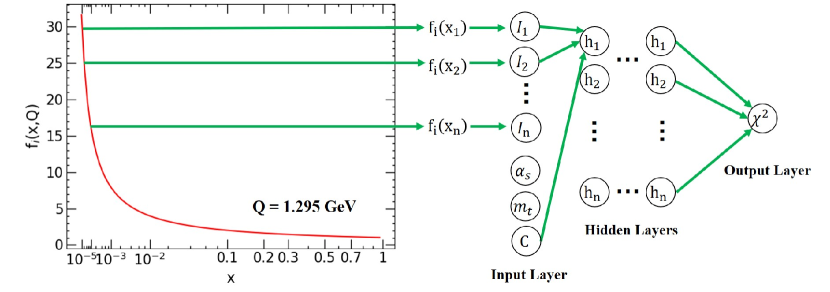
Figure 1: An example of the architecture of NNs adapted in this work, taking $\chi^{2}$ as the target function. Inputs to the NN include the flavor-dependent PDFs at discrete values of $x$ (e.g., $x_{l}\!\in\![0,1])$; pQCD parameters, namely, the top-quark mass, $m_{t}$, and strong coupling constant, $\alpha_{s}$; and the SMEFT Wilson coefficients.

A training sample consisting of 12000 PDF replicas with different $\alpha_{s}$ values, and associated inputs of $m_{t}$, $C_{1}$, and one of $\{C_{tu}^{1},C_{tq}^{8}$, $C_{tG}\}$ is generated. The $\alpha_{s}$, $m_{t}$, $C_{1}$, and $\{C_{tu}^{1},C_{tq}^{8}$, $C_{tG}\}$ values are generated randomly from uniform distributions defined over reasonably-chosen domains of interest. Details on the generation of PDF replicas are described in Ref. 2201.06586 . We compute the $\chi^{2}$ of all the data sets for each of the replicas according to the theoretical choices described above. We train each NN for 12 hours on a single CPU-core (2.4 GHz) which is sufficient to obtain the necessary accuracy, as we discuss below.

3.3 Validating the neural network

The accuracy of the prescribed NNs used in this study has already been validated thoroughly in Ref. 2201.06586 when using only PDF values as inputs at the first layer. We generate an independent 4000-replica test sample to validate the performance of the NN so as to prevent over-training and crosscheck the statistical agreement of predictions based on the NN output with the true parametric shape of the underlying $\chi^{2}$ function. In the end, we find equally good performance for all data sets considered in this work using the updated architecture outlined above with the additional SM parameters and SMEFT inputs. For example, we consider the data sets involving top-quark pair production and define $\chi^{2}_{t\bar{t}}$ to be the sum of the individual $\chi^{2}$ values for each of the 5 data sets used in our nominal fit as summarized in Tab. 3. In Fig. 2, we show histograms based on the 4000 PDF replicas in the test sample giving the ratio of the $\chi^{2}_{t\bar{t}}$ prediction from the trained NNs to the true value from direct computation. We note that the $\chi^{2}$ predicted for the full data set is obtained by summing the respective outputs of the NNs. The resulting distribution is then normalized to the total number of the replicas included in the test sample. Post-training, the NN predictions agree with the true $\chi^{2}$ calculation to much better than sub-percent accuracy — within 4 per-mille; the deviations from $\chi^{2}_{\mathrm{NN}}/\chi^{2}\!=\!1$ exhibit an approximately Gaussian distribution.

In Fig. 3, we show the ratio of the $\chi^{2}_{t\bar{t}}$ prediction based on the NN output to its true value for each of the PDF replicas in the test sample, in this case plotted against select SM parameters and the true $\chi^{2}$; namely, every PDF replica is associated with a corresponding value of $\alpha_{s}$, $m_{t}$ and $C_{tu}^{1}$, and the associated $\chi^{2}_{t\bar{t}}$. While there is an a sub-permille shift in the direction of $\chi^{2}_{\mathrm{NN}}\!>\!\chi^{2}$ as well as extremely soft oscillations in the $m_{t}$ plot, the panels in Fig. 3 otherwise reveal no significant dependence of the $\chi^{2}_{\mathrm{NN}}/\chi^{2}$ ratio upon the input parameters. This behavior confirms that the NNs indeed reproduce the local dependence of the likelihood function on the SM parameters introduced in this study, with no evidence of systematic, parameter-dependent deviations from the true $\chi^{2}$. The distribution of $\chi^{2}_{t\bar{t}}$ for the 4000-replica training set is bounded within [40, 330] $\chi^{2}$-units, and the absolute deviations of the NN predictions are generally within 0.1 unit, especially when close to the global minimum. This level of agreement is sufficiently accurate for a global analysis.

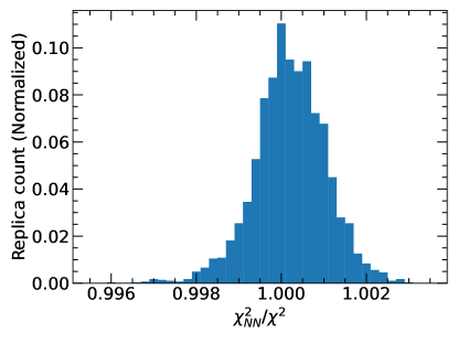
Figure 2: A histogram giving the ratio of $\chi^{2}_{t\bar{t}}$ as predicted by NNs to the true value from direct calculation for all 4000 PDF replicas in the test sample. The distribution is normalized to the total number of the replicas included in the test sample.

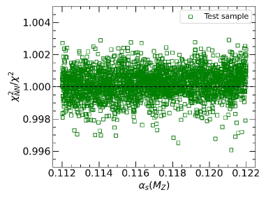
((a))

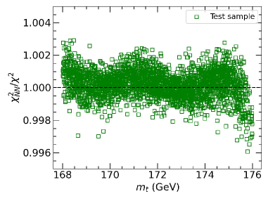
((b))

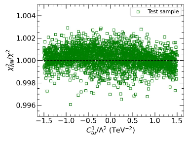
((c))

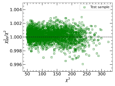
((d))

Figure 3: The ratio of the $\chi^{2}_{t\bar{t}}$ prediction by NNs to its truth for each of the PDF replica in the test sample, distributed in the variable $\alpha_{s}$, $m_{t}$, $C_{tu}^{1}$ and $\chi^{2}_{t\bar{t}}$, respectively.

3.4 Method of LM scans

The Lagrange multiplier (LM) method hep-ph/0008191 ; hep-ph/0101051 is a robust approach for estimating the uncertainty of any dependent variable $X(\{a_{\ell}\})$, where $\{a_{\ell}\}$ represent the free parameters in the global analysis as before. In this method, the $\chi^{2}$ of the global fit is modified by introducing the derived variable, $X(\{a_{\ell}\})$, of the underlying fit parameters as a LM constraint. The new function to be minimized in the global fit is then given by the sum of two parts,

$$\Psi\left(\lambda,\left\{a_{\ell}\right\}\right)\equiv\chi^{2}\left(\left\{a_{\ell}\right\}\right)+\lambda X\left(\left\{a_{\ell}\right\}\right),$$ (10)

where $\lambda$ is the Lagrange multiplier, which can be continuously varied. For each value of $\lambda$, one can determine a set of $\{a_{\ell}\}$, $X(\{a_{\ell}\})$ and $\chi^{2}(\{a_{\ell}\})$ by minimizing $\Psi$, such that the corresponding $\chi^{2}(\{a_{\ell}\})$ then represents the lowest possible $\chi^{2}$ for the corresponding value of the $X(\{a_{\ell}\})$. The best-fit value of $X(\{a_{\ell}\})$ and the global minimum, $\chi^{2}_{min}$, correspond to the choice $\lambda$ = 0 in Eq. (10). By repeating the minimization for different values of $\lambda$, one can determine sets of $\{a_{\ell}\}$, $X(\{a_{\ell}\})$ and $\chi^{2}(\{a_{\ell}\})$. With this information, it is possible to determine the profiled $\chi^{2}$ as a function of the variable $X$, and the PDF uncertainty of $X$ at the 90% CL may be evaluated against a tolerance criteria, $\Delta\chi^{2}\!+\!P\!\leq\!100$, following the CT18 default analysis. The penalty term $P$, called the Tier-2 penalty 1709.04922 , is introduced to ensure the tolerance is saturated as soon as any data set shows disagreement at the 90% CL. We point out that in the special case in which $X(\{a_{\ell}\})$ is simply taken to be one of the input parameters, $a_{\ell}$, of the global fit, the LM scan is equivalent to repeating the fit with one of $a_{\ell}$ systematically fixed to different values.

The correlation between two dependent variables, $X_{1}(\{a_{\ell}\})$ and $X_{2}(\{a_{\ell}\})$, can be assessed with two-dimensional (2D) LM scans 2201.06586 , which can be achieved by simultaneously introducing both $X_{1}(\{a\})$ and $X_{2}(\{a\})$ via Lagrange multipliers. The new function to be minimized in this case is a straightforward generalization of Eq. (10), becoming

$$\Psi\left(\lambda_{1},\lambda_{2},\left\{a_{\ell}\right\}\right)\equiv\chi^{2}\left(\left\{a_{\ell}\right\}\right)+\lambda_{1}{X_{1}}\left(\left\{a_{\ell}\right\}\right)+\lambda_{2}{X_{2}}\left(\left\{a_{\ell}\right\}\right),$$ (11)

where $\lambda_{1}$ and $\lambda_{2}$ are the specified LM constants as before. One can determine the profiled $\chi^{2}$ as a function of the variables $X_{1}$ and $X_{2}$. The resulting 2D manifold for $\Delta\chi^{2}$ in the plane of $X_{1}$ vs. $X_{2}$ can be read as a traditional contour plot, quantifying the correlation between $X_{1}$ and $X_{2}$.

4 Experimental data

In this section, we briefly summarize the relevant experimental data sets in our simultaneous global analysis of QCD and SMEFT. We start with the CT18 NNLO fit as a baseline by including all 39 default data sets from this study, consisting of DIS and DY as well as top-quark pair and jet production. We then include several additional LHC experiments at 8 and 13 TeV — specifically, distributions from top-quark pair and jet production; we also incorporate total cross section data for top-quark pair production at both the Tevatron and LHC. BSM scenarios parametrized through SMEFT are directly constrained in particular by the 13 data sets on top-quark pair and jet production as summarized in Tab. 3. Additional detail regarding the other 32 data sets on DIS and DY production can be found in Ref. 1912.10053 . In Tab. 3, sets marked with a star (dagger) are included in our nominal PDF+SMEFT fits of top-quark pair (jet) production data. We further summarize key aspects of these experiments, including their respective kinematical coverages, in the subsections below.

Experiments	$\sqrt{s}$(TeV)	$\mathcal{L}(\text{fb}^{-1})$	observable		$N_{\text{pt}}$
∗† LHC(Tevatron)	7/8/13(1.96)	—	$t\bar{t}$ total cross section	1309.7570 ; 1406.5375 ; 1208.2671 ; 1603.02303 ; ATLAS-tot-13 ; 1611.04040	8
∗† ATLAS $t\bar{t}$	8	20.3	1D dis. in $p_{T,t}$ or $m_{t\bar{t}}$	1511.04716	15
∗† CMS $t\bar{t}$	8	19.7	2D dis. in $p_{T,t}$ and $y_{t}$	1703.01630	16
CMS $t\bar{t}$	8	19.7	1D dis. in $m_{t\bar{t}}$	1505.04480	7
∗† ATLAS $t\bar{t}$	13	36	1D dis. in $m_{t\bar{t}}$	1908.07305	7
∗† CMS $t\bar{t}$	13	35.9	1D dis. in $m_{t\bar{t}}$	1811.06625	7
∗† CDF II inc. jet	1.96	1.13	2D dis. in $p_{T}$ and $y$	0807.2204	72
∗† D0 II inc. jet	1.96	0.7	2D dis. in $p_{T}$ and $y$	0802.2400	110
∗† ATLAS inc. jet	7	4.5	2D dis. in $p_{T}$ and $y$	1410.8857	140
∗† CMS inc. jet	7	5	2D dis. in $p_{T}$ and $y$	1406.0324	158
∗ CMS inc. jet	8	19.7	2D dis. in $p_{T}$ and $y$	1609.05331	185
† CMS dijet	8	19.7	3D dis. in $p_{T}^{ave.}$, $y_{b}$ and $y^{*}$	1705.02628	122
† CMS inc. jet	13	36.3	2D dis. in $p_{T}$ and $y$	2111.10431	78

Table 3: Experimental data sets on top-quark pair and jets production included in the global analyses. $N_{\text{pt}}$ indicates the total number of data points in each data set. The data sets marked with star (dagger) are included in our nominal fits for study of SMEFT in top-quark pair (jet) production. Other data sets on DIS and DY productions are the same as in CT18 analyses and are not shown here for simplicity.

4.1 Top-quark pair production

The ATLAS and CMS collaborations at the LHC have measured differential cross sections for top-quark pair production in several kinematic variables at ${\sqrt{s}}=8$ TeV. With the exception of ATLAS, we avoid including multiple distributions from the same experiment due to the complicated and hard-to-control statistical correlations which would exist among these data sets. For ATLAS, however, we include one-dimensional distributions in both the invariant mass of the top-quark pair, $d\sigma/dm_{t\bar{t}}$, and the transverse momentum of the top quark, $d\sigma/dp_{T,t}$, corresponding to an integrated luminosity of $\mathcal{L}\!=\!20.3\,\mathrm{fb}^{-1}$ 1511.04716 ; this results in 8 and 7 data points, respectively. For CMS, with $\mathcal{L}\!=\!19.7\,\mathrm{fb}^{-1}$ of integrated luminosity, we nominally fit the normalized double-differential cross section, $(1/\sigma)\times d^{2}\sigma\big{/}dp_{T,t}\,dy_{t}$ 1703.01630 . These data sets were included in the CT18 fit as Exp. ID# 580 and 573, respectively. As mentioned earlier, in our variant fit the CMS measurement of the normalized differential cross section, $(1/\sigma)\times d\sigma/dm_{t\bar{t}}$ 1505.04480 , is used instead. We also note that the kinematic reach of these data was restricted to $p_{T,t}\!<\!600$ GeV and $m_{t\bar{t}}\!<\!1600$ GeV.

For $\sqrt{s}\!=\!13$ TeV, we select the distribution on $m_{t\bar{t}}$ on the logic that the large $m_{t\bar{t}}$ region is more sensitive to BSM physics. In this case, the ATLAS data we fit 1908.07305 were collected in 2015 and 2016 with $\mathcal{L}\!=\!36$ $\text{fb}^{-1}$ in the lepton+jet decay channel of the top-quark pair. For CMS 1811.06625 , the data were collected in 2016, corresponding to an integrated luminosity of 35.9 $\text{fb}^{-1}$ in the dilepton decay channel. The two collaborations provide measurements based on the same binning scheme over $m_{t\bar{t}}$ with bin edges located at $[300,380,470,620,820,1100,1500,2500]~{}\text{GeV}$; this therefore results in $N_{\mathrm{pt}}\!=\!7$ for both experiments.

Lastly, we have also taken into account measurements of the $t\bar{t}$ total cross section from the Tevatron and LHC (for the latter, with $\sqrt{s}\!=\!7,8,13$ TeV), leading to a combined total of 8 more data points. To be specific, we include the data from CDF and D0 at $\sqrt{s}=1.96$ TeV 1309.7570 ; ATLAS 1406.5375 ($e\mu$ channel) and CMS 1208.2671 (dilepton channel) at $\sqrt{s}=7$ TeV; ATLAS 1406.5375 ($e\mu$) and CMS 1603.02303 ($e\mu$) at $\sqrt{s}=8$ TeV; and ATLAS ATLAS-tot-13 ($e\mu$) and CMS 1611.04040 ($e\mu$) at $\sqrt{s}=13$ TeV. The precision of these measurements ranges from 2% for ATLAS at 13 TeV to 8% for D0.

4.2 Inclusive jet and dijet production

For inclusive jet production we include data on the double-differential cross section in the transverse momentum and rapidity of the jet, $d^{2}\sigma/(dp_{T}\,dy)$, as measured by the CDF and D0 experiments during Run-II of the Tevatron. The CDF experiment measured the inclusive jet cross section in $p\bar{p}$ collisions at $\sqrt{s}=1.96$ TeV with data corresponding to an integrated luminosity of $1.13~{}\text{fb}^{-1}$ 0807.2204 . This measurement used the cone-based midpoint jet-clustering algorithm in the jet rapidity region of $|y|<2.1$, with a cone radius $R\equiv\sqrt{(\Delta y)^{2}+(\Delta\phi)^{2}}=0.7$ in rapidity $y$ and azimuthal angle $\phi$, resulting in 72 data points in total. Meanwhile, the D0 experiment collected a data sample at a center-of-mass-energy of $\sqrt{s}=1.96$ TeV, corresponding to an integrated luminosity of 0.70 $\text{fb}^{-1}$ 0802.2400 . Cross sections on inclusive jet production with jet transverse momenta from 50 to 600 GeV and jet rapidities of up to 2.4 were divided into 110 bins. Again, the midpoint jet algorithm with radius $R=0.7$ was adopted.

For ATLAS, measurements of inclusive jet production at $\sqrt{s}=7$ TeV based on the anti-$k_{T}$ jet algorithm 0802.1189 with radius $R=0.6$ are included in our fit, where these data have an integrated luminosity of 4.5 $\text{fb}^{-1}$ 1410.8857 . This set covers a jet rapidity range of $0\leq|y|\leq 3.0$ and associated transverse momentum range of $74\leq p_{T}\leq 1992$ GeV, for a total of 140 data points. For CMS, we fit inclusive jet data measured at $\sqrt{s}=7$ TeV 1406.0324 , 8 TeV 1609.05331 and 13 TeV 2111.10431 , with these corresponding to $\mathcal{L}\!=\!5$, 19.7 and 36.3 $\text{fb}^{-1}$, respectively. The 7 TeV set contains 158 data points, covering a phase-space region with jet transverse momentum 56 $\leq p_{T}\leq$ 1327 GeV, and rapidity $0\leq|y|\leq 3.0$. For the 8 TeV data, there are a total of 185 points, in this case covering transverse momenta 74 $\leq p_{T}\leq$ 2500 GeV and jet rapidities over $0\leq|y|\leq 3.0$. Finally, the 13 TeV data set involves 78 points, covering a phase space region with jet transverse momentum from 97 GeV up to 3.1 TeV and rapidity $|y|\leq 2.0$. We stress that the CMS 8 TeV jet data are only used in the variant SMEFT fit for jet production. In our nominal fit, however, we instead use the CMS dijet measurements recorded at 8 TeV 1705.02628 . These measurements provide 122 data points on the triple-differential cross section, which is dependent on the average transverse momentum of the two leading jets, $p_{T,\text{avg}}\equiv(p_{T,1}+p_{T,2})/2$; half of their rapidity separation, $y^{*}\equiv|y_{1}-y_{2}|/2$; and the rapidity of the dijet system, $y_{b}\equiv|y_{1}+y_{2}|/2$. In this case, the average transverse momentum can reach 1600 GeV in the central rapidity region, and we point out that, for all CMS measurements, we select those data which were measured using the anti-$k_{T}$ algorithm with a jet radius $R=0.7$.

5 LM scans with top-quark pair production

In this section, we investigate the determination of the top-associated SMEFT Wilson coefficients [corresponding to the operators of Eq. (2)] in our combined analysis with PDF degrees-of-freedom; we quantify constraints on the SMEFT coefficients via LM scans as discussed in Sec. 3.4. Before doing this, however, we first examine the impact of our fitted data on the purely SM input parameters, namely, the top-quark mass, $m_{t}$, and the strong coupling constant, $\alpha_{s}(M_{Z})$, given that these quantities are strongly correlated with top-quark pair production. We note that the other default data sets for jet production and DIS/DY are always included in our global analyses as well, although these information do not impose as direct constraints, particularly with respect to $m_{t}$.

5.1 Impact of strong coupling and top-quark mass

We first carry out a series of LM scans on a joint fit of PDFs, $m_{t}$ and $\alpha_{s}(M_{Z})$ — without considering SMEFT contributions. In Fig. 4 (a) and (b), we show the profiled $\chi^{2}$ as a function of $\alpha_{s}(M_{Z})$ and $m_{t}$, respectively. The black-solid line(s) represent the change, $\Delta\chi^{2}$, in the global likelihood function relative to the best fit, $\Delta\chi^{2}\!=\!0$, whereas the various colorful dot, dash and dot-dash curves represent the contributions to $\Delta\chi^{2}$ from individual experimental data sets. We find that both the global and individual experimental $\Delta\chi^{2}$ curves show an almost quadratic dependence on the variables in the neighborhood of the global minimum.

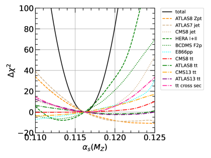
((a))

((b))

Figure 4: LM scans on $\alpha_{s}(M_{Z})$ (left panel) and $m_{t}$ (right panel). The black-solid lines represent the total $\Delta\chi^{2}$ of the global fit. The dotted, dashed, and dot-dashed curves represent the contributions to $\Delta\chi^{2}$ from individual experimental data sets.

In Fig. 4 (a) for $\alpha_{s}(M_{Z})$, we see that, as expected, the combined HERA DIS data stand out as providing an especially important constraint due to both the high experimental precision and large volume of data for this set. The LM scans predict a value of $\alpha_{s}(M_{Z})=0.1162$, which is slightly smaller than, but consistent with, the world average of $\alpha_{s}(M_{Z})=0.1179\pm 0.001$ Workman:2022 . These results on $\alpha_{s}(M_{Z})$ are also consistent with those reported in the CT18 analysis and serve as a crosscheck on the accuracy of our new approach based on NNs. Meanwhile, in Fig. 4 (b) the LM scans over $m_{t}$ show that the $t\bar{t}$ data offer the dominant constraint(s), again as expected. The LM scans predict a central value and uncertainty of $m_{t}=172.58$ GeV, which is slightly larger than the world average of $m_{t}=172.4\pm 0.7$ GeV Workman:2022 from measurements of cross sections; still, up to uncertainties, these values are nicely consistent. We find that both the CMS 8 and 13 TeV $t\bar{t}$ data prefer a smaller value of $m_{t}$ compared to the ATLAS $t\bar{t}$ data, which prefer larger $m_{t}$, much as was reported in Ref. 1904.05237 , which attributed these preferences as mainly coming from constraints provided by the first kinematic bin of the $m_{t\bar{t}}$ distribution close to the threshold region. A detailed study on determination of the top-quark mass will be presented elsewhere.

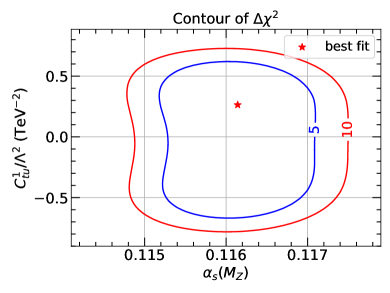
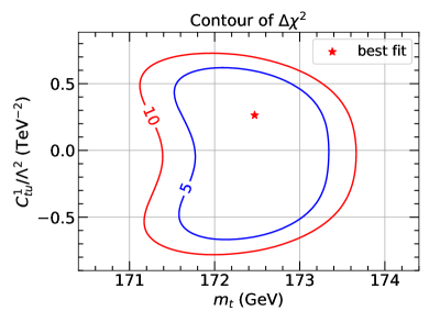
Figure 5: Contour plot of $\Delta\chi^{2}$ in the plane of $C^{1}_{tu}$ vs. $\alpha_{s}(M_{Z})$ [left] and $C^{1}_{tu}$ vs. $m_{t}$ [right], as determined according to the 2D LM scan technique of Eq. (11) and surrounding text.

$\chi^{2}$ (nominal)	tot. cross sect.	CMS 8	ATLAS 8	CMS 13	ATLAS 13	global
all free	5.08	16.70	11.41	14.24	4.73	4278.62
$m_{t}$ fixed	5.09	16.76	11.30	14.30	4.71	4278.63
$\alpha_{s}$ fixed	6.13	17.27	9.85	15.96	4.13	4297.38
$\alpha_{s}$ and $m_{t}$ fixed	6.91	16.52	10.95	15.06	4.47	4297.97
all fixed	6.90	16.49	11.03	14.62	4.96	4298.03

Table 4: Central values of $\chi^{2}$ for the individual $t\bar{t}$ data sets as well as the full global fit assuming various fixing conditions on the parameters $\alpha_{s}(M_{Z})$, $m_{t}$, and $C_{tu}^{1}$.

Following these preliminaries on the purely SM fits, we now move to joint SMEFT/SM fits, taking $C^{1}_{tu}$ as a first example. A priori, it is possible that significant parametric correlations might exist among the PDF and SM input parameters illustrated above and the SMEFT operator coefficients. To investigate this potential interplay, we simultaneously consider the Wilson coefficient and $\alpha_{s}(M_{Z})$ or $m_{t}$ in the two panels of Fig. 5, showing the contours of $\Delta\chi^{2}$ in the plane of $C^{1}_{tu}$ vs. $\alpha_{s}(M_{Z})$ (left panel) and $C^{1}_{tu}$ vs. $m_{t}$ (right) based on the 2D LM scans of Eq. (11). Here, the blue and red contours represent $\Delta\chi^{2}=$ 5 and 10, respectively. For the fitted data set, we find only very minimal correlations between $C^{1}_{tu}$ and $\alpha_{s}(M_{Z})$ or $m_{t}$, consistent with the SM, corresponding to $C^{1}_{tu}=0$. In fact, the best-fit values of $\alpha_{s}(M_{Z})$ and $m_{t}$ are almost identical (and well within a small $\Delta\chi^{2}$ interval) to those shown in Fig. 4, which corresponded to fitting without SMEFT contributions. We note that the shapes of the contours are mildly asymmetric because of the non-quadratic dependence of $\chi^{2}$ on the underlying parameters. These conclusions also hold for the other top-associated Wilson coefficients of Eq. (2).

To further disentangle possible correlations among the SM/EFT input parameters impacting the description of the $t\bar{t}$ data, we perform a series of global fits with either $\alpha_{s}(M_{Z})$ fixed to 0.118 or $m_{t}$ fixed to 172.5 GeV, with both of these fixed, or with $C^{1}_{tu}$ fixed to 0. The resulting $\chi^{2}$ values under these scenarios for the various individual $t\bar{t}$ data sets as well as the total at the global minimum are summarized in Tab. 4. The total $\chi^{2}$ is elevated by about 18 units if $\alpha_{s}(M_{Z})$ is fixed to 0.118, consistent with results shown in Fig. 4, while it changes by less than one unit when fixing $m_{t}$ or $C^{1}_{tu}$ as call be deduced from the “all fixed” scenario of Tab. 4. The $\chi^{2}$ of individual $t\bar{t}$ data sets only change slightly with shifts in opposing directions depending on the specific data set. The sum of $\chi^{2}$ from all $t\bar{t}$ data sets varies within 2 units as a consequence.

We conclude that varying $\alpha_{s}(M_{Z})$ and $m_{t}$ away from their respective world averages has little impact on extractions of SMEFT Wilson coefficients, provided these variations remain within present uncertainties. Below, we present LM scans to further explore constraints on the SMEFT coefficients; for these, we perform joint fits of PDFs and Wilson coefficients only, fixing $\alpha_{s}(M_{Z})=0.118$ and $m_{t}=172.5$ GeV. Lastly, we have also checked the impact of the resummed Coulomb corrections mentioned in Sec. 2, and we find these corrections have a negligible effect upon determinations of the Wilson coefficients.

5.2 Four-quark and gluonic operators

We first show results for the four-quark operators, $O_{tu}^{1}$ and $O_{td}^{1}$. We perform LM scans on a single effective Wilson coefficient, assuming $C_{tu}^{1}=C_{td}^{1}$, with all other SMEFT coefficients set to zero as discussed earlier. The profiled $\chi^{2}$ as a function of $C_{tu}^{1}$ is shown in Fig. 6. We find that both the global $\Delta\chi^{2}$ and the $\Delta\chi^{2}$ curves for individual experiments show a predominantly quartic dependence on $C_{tu}^{1}$, which is expected since the interference between the SM and the SMEFT operators, $O_{tu}^{1}$ and $O_{td}^{1}$, starts at NLO in QCD.

In the left panel of Fig. 6 we present the nominal calculation — i.e., with default scale choices and uncertainties as discussed in Sec. 2.2 — finding that the 13 TeV CMS $t\bar{t}$ data impose the strongest constraint under this scenario, showing the most rapid growth in $\Delta\chi^{2}$, especially for larger values of $|C_{tu}^{1}|$. Intriguingly, the 13 TeV ATLAS $t\bar{t}$ data suggest a tiny preference for nonzero $|C_{tu}^{1}/\Lambda^{2}|$, with a $\sim\!2$-unit $\Delta\chi^{2}$ dip in the neighborhood of $|C_{tu}^{1}/\Lambda^{2}|\!\sim\!(0.5-0.6)$ TeV^-2 relative to the zero-SMEFT baseline; this, coupled with the comparatively slow growth in $\Delta\chi^{2}$ seen for the other $t\bar{t}$ sets, has the effect of broadening the total uncertainty allowed for this SMEFT Wilson coefficient. Still, the uncertainty range is mostly determined by the penalty term of this data set. The LM scans ultimately predict a result of $C_{tu}^{1}/\Lambda^{2}=0.14^{+0.61}_{-0.97}$ TeV^-2 at 90% CL, which is consistent with the SM. Analogously, in the right panel we show the corresponding results determined without theoretical scale-choice uncertainties. We find that the behaviors of both global $\Delta\chi^{2}$ and individual experimental $\Delta\chi^{2}$ are very similar to those shown in the left panel, but with a modest increase in the takeoff of $\Delta\chi^{2}$, particularly in the tails of the profiled experiments. This implies a slight reduction in the uncertainties for $C_{tu}^{1}/\Lambda^{2}$, as is to be expected. In addition to Fig. 6, we also perform LM scans on $C_{tu}^{1}$ under the scenario that the PDF parameters are fixed to values at the global minimum. This leads to $C_{tu}^{1}/\Lambda^{2}=0.14^{+0.60}_{-0.95}$ TeV^-2 at 90% CL, which is very close to the results with the nominal setup, indicating that correlations between the PDFs and $C_{tu}^{1}$ are indeed weak when fitted to present data.

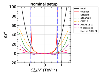
((a))

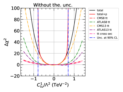
((b))

Figure 6: LM scans on $C_{tu}^{1}/\Lambda^{2}$ ($=\!C_{td}^{1}/\Lambda^{2}$) under the nominal fit (left panel) as well as excluding theoretical scale-choice uncertainties (right panel). The solid black and red lines represent $\Delta\chi^{2}$ and $\Delta\chi^{2}+P$, respectively. The dot-dashed curves represent the contributions to $\Delta\chi^{2}$ from individual experimental data sets. The blue vertical dot-dashed lines indicate the 90% CL uncertainties as determined by requiring $\Delta\chi^{2}+P=100$.

In Fig. 7, we compare the gluon PDF, $g(x,Q_{0})$, at $Q_{0}$ = 1.295 GeV determined by fitting with and without BSM SMEFT contributions from the inclusion of $O_{tu}^{1}\!=\!O_{td}^{1}$. We also show the $g$-PDF determined without theoretical uncertainties as also explored in Fig. 6. In the left panel, the blue and red solid lines represent the central values of the gluon PDF determined with [SM+$C^{1}_{tu}$] and without [SM] nonzero SMEFT contributions, respectively. The green-solid line represents the central value of the $g$-PDF when determined in the presence of nonzero SMEFT but without theoretical uncertainties. The PDF uncertainties at 68% CL are shown as hatched areas in the various relevant colors. We find that the fitted gluon PDFs obtained with and without BSM as parametrized by SMEFT are almost indistinguishable in terms of both the central value and uncertainty. We note a very slight upward shift in the central value of the PDF, and corresponding $\sim\!7\%$ reduction in the uncertainty, for $x\!\sim\!0.02$ once theoretical uncertainties are removed. In addition, a slight downward shift in the central gluon PDF, of relative magnitude $\lesssim\!5\%$ and with a $\sim\!10\%$ narrowing of the uncertainty, occurs near $x\!\sim\!0.5$. As a companion plot, in the right panel of Fig. 7 we show the relative PDF uncertainties at 68% CL for each of the curves discussed above, now normalized to the nominal SM fit so as to more clearly illustrate the effect on the size of the PDF errors of incorporating SMEFT coefficients and (not) including theoretical uncertainties.

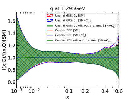
((a))

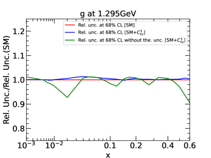
((b))

Figure 7: The gluon PDFs, $g(x,Q)$, determined by fitting with and without BSM contributions from $O_{tu}^{1}$ and $O_{td}^{1}$ at $Q=1.295$ GeV are shown in the left panel. The blue and red solid lines represent the central values determined by fitting with and without SMEFT contributions respectively, and the green solid line represents the central value determined by fitting with SMEFT contributions and without theoretical uncertainties. The PDF uncertainties at 68% CL are shown through hatched areas with relevant colors. The relative uncertainties are shown in the right panel with the same colors.

We next turn our focus to another of the four-quark operators of Eq. 2, $O_{tq}^{8}$. In Fig. 8 we show the results of LM scans on $C_{tq}^{8}$. As before, in the left panel we show the result of the calculation based on our nominal fit configuration, in this case finding strong constraints from the 8 and 13 TeV CMS data as well as the total $t\bar{t}$ cross section measurements. In the nominal fit, we treat PDF parameters and EFT coefficients on the same footing and thus consistently obtain bounds on EFT coefficients with PDF uncertainties inside the framework of CT18. As had been the case for $C_{tu}^{1}$, there is a very small hint of a preference for a nonzero SMEFT Wilson coefficient from both the 8 and 13 TeV ATLAS data, but these largely lie at values suppressed by the penalty term of the likelihood function, which again plays a decisive role in the full uncertainty on $C_{tq}^{8}/\Lambda^{2}$. The LM scans predict a result of $C_{tq}^{8}/\Lambda^{2}=-0.80^{+2.58}_{-2.38}$ TeV^-2 at 90% CL. In the right panel of Fig. 8, the PDF parameters are fixed to their values at the global minimum. Hence, the PDF uncertainties are not included in the bounds on EFT coefficients. The LM scans predict a result of $C_{tq}^{8}/\Lambda^{2}=-0.80^{+2.48}_{-2.35}$ TeV^-2 at 90% CL with uncertainties slightly smaller than those shown in the left panel. As before, this suggests only very mild correlations between SMEFT and PDF parameters at the current time, but with a mild possibility of slightly underestimating the full uncertainty on SMEFT Wilson coefficients in analyses with fixed PDF degrees-of-freedom.

The SMEFiT collaboration presents a global interpretation of Higgs, diboson, and top-quark production and decay measurements from the LHC in the framework of the SMEFT 2105.00006 . The 95% CL bound associated with the one-parameter EFT fits for $C_{tq}^{8}/\Lambda^{2}$ is [-0.483, 0.393] TeV^-2. In our PDF fixed case, the 95% CL bound determined with the same parameter-fitting criterion as Ref. 2105.00006 is [-2.285, 0.701] TeV^-2, which is slightly weaker than the SMEFiT result. The main reason for this is that the SMEFiT study included more experimental data sets with larger luminosity. In this work, we only consider 5 data sets involving top-quark pair production, amounting to a total integrated luminosity of $\mathcal{L}\!\sim$111.9 fb^-1. The total number of top quark-pair sets included in the SMEFiT study is 9, and the total integrated luminosity is $\sim\!193$ fb^-1. Also relevant is the fact that the scale uncertainties on the $t\bar{t}$ production cross sections were not considered in Ref. 2105.00006 .

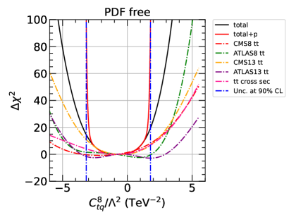
((a)) PDF free

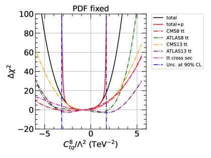
((b)) PDF fixed

Figure 8: LM scans on $C_{tq}^{8}/\Lambda^{2}$ with the PDF parameters allowed to free vary (left panel) or fixed at the global minimum (right panel).

In Fig. 9, we compare gluon PDFs at $Q_{0}$ = 1.295 GeV as determined by fits with and without the freely-varying SMEFT contributions from $O_{tq}^{8}$. The PDF uncertainties at 68% CL are shown through hatched areas with relevant colors. In the left panel, we find that the PDFs from the two fits are almost indistinguishable for both the central value and the uncertainty region. A negligible upward shift smaller than 1% on the central value can be seen in the endpoint regions of $x\lesssim 3\times 10^{-3}$ and $x\gtrsim 0.5$ after including possible BSM contributions via the SMEFT coefficient. In the right panel, the size of the relative PDF uncertainty is modestly enlarged at the $\sim\!5\%$ level around $x\!\sim\!0.03$ following the inclusion the fitted SMEFT coefficient.

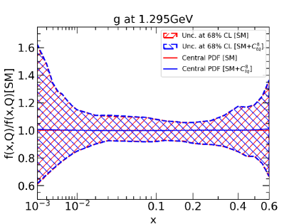
((a))

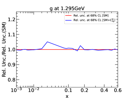
((b))

Figure 9: The $g$ PDFs determined by fitting with and without SMEFT contributions from $O_{tq}^{8}$ at $Q_{0}=1.295$ GeV are shown in the left panel. The blue and red solid lines represent the central values determined by fitting with and without BSM contributions, respectively. The PDF uncertainties at the 68% CL are shown through hatched areas in the relevant colors. The relative 68%-level uncertainties, normalized to the purely SM scenario, are shown in the right panel in matching colors.

Lastly, we also consider the other top-relevant (gluonic) operator, $O_{tG}$, showing in Fig. 10 the analogous LM scan results on $C_{tG}$. For the nominal setup, given in the left panel, we find that the constraint from the total cross section measurements predominate among the various fitted experiments; as before, the uncertainty on $C_{tG}/\Lambda^{2}$ mostly comes from the penalty term of this data set, such that the LM scans predict a result of $C_{tG}/\Lambda^{2}=-0.10^{+0.26}_{-0.30}$ TeV^-2 at 90% CL. In the right panel, the PDF parameters are fixed to their values at the global minimum. The result in this case, $C_{tG}/\Lambda^{2}=-0.10^{+0.25}_{-0.30}$ TeV^-2 at 90% CL, is again closely to that obtained under the nominal setup. This once again indicates a weak correlation between PDFs and $C_{tG}$ in the global fit. We also note that, unlike the corresponding LM scans for $C^{1}_{tu}/\Lambda^{2}$ and $C^{8}_{tq}/\Lambda^{2}$ shown earlier, $\Delta\chi^{2}$ mostly grows monotonically away from the $C\!=\!0$ SM scenario, with minima of only extremely shallow depth for, e.g., the 8 and 13 TeV ATLAS $t\bar{t}$ experiments. The SMEFiT collaboration reports a 95% CL bound on $C_{tG}/\Lambda^{2}$ of [0.006, 0.107] TeV^-2 from the one-parameter EFT fits 2105.00006 . In our case when using the same criterion for the PDF fixed case, we obtain a bound of [-0.255, 0.052] TeV^-2 at 95% CL, which is again weaker for the reasons summarized before.

We summarize the results we obtain for all three Wilson coefficients under different fitted assumptions in Tab. 5. In Fig. 11, we compare $g$ PDFs at $Q_{0}$ = 1.295 GeV determined by fitting with and without SMEFT contributions from $O_{tG}$, finding that these fits are essentially indistinguishable. We therefore conclude that, at present, SMEFT-PDF correlations in the $t\bar{t}$ sector are effectively absent for $O^{1}_{tu}$ (=$O^{1}_{td}$) and $O_{tG}$, while nonzero but very weak for the octet operator, $O^{8}_{tq}$.

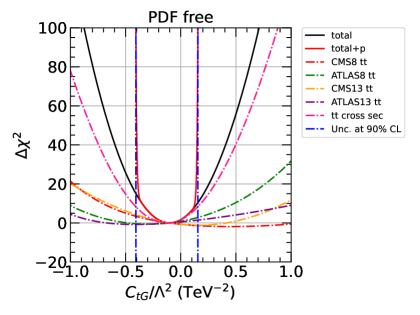
((a))

((b))

Figure 10: LM scans over $C_{tG}/\Lambda^{2}$ with the PDF parameters freely varying (left panel) or fixed to their best-fit values (right panel).

TeV-2	nominal	PDF fixed	no the. unc.
$C_{tu}^{1}/\Lambda^{2}$	$0.14^{+0.61}_{-0.97}$	$0.14^{+0.60}_{-0.95}$	$0.14^{+0.57}_{-0.92}$
$C_{tq}^{8}/\Lambda^{2}$	$-0.80^{+2.58}_{-2.38}$	$-0.80^{+2.48}_{-2.35}$	-
$C_{tG}/\Lambda^{2}$	$-0.10^{+0.26}_{-0.30}$	$-0.10^{+0.25}_{-0.30}$	-

Table 5: Constraints on new physics at 90% CL.

((a))

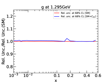
((b))

Figure 11: The $g$-PDFs determined by fitting with and without SMEFT contributions via $O_{tG}$ at $Q_{0}=1.295$ GeV are shown in the left panel. The blue and red solid lines represent the central values determined by fitting with and without BSM contributions respectively. The PDF uncertainties at 68% CL are shown through hatched areas with the corresponding colors. The relative uncertainties at 68% CL are shown in the right panel, normalized to the SM curve.

We evaluate the constraints on the Wilson coefficients from each $t\bar{t}$ experiment by repeating the global fit, retaining only a single data set at a time. The results of this procedure are listed in Tab. 6. The second column shows the results obtained through the full data set fitted under nominal settings. For $C_{tu}^{1}/\Lambda^{2}$, given in the first row, the CMS 13 TeV data the give strongest constraint, consistent with the $\Delta\chi^{2}$ profiles shown in Fig. 6. In addition, the ATLAS 8 and 13 TeV data both prefer a positive $C_{tu}^{1}/\Lambda^{2}$. For $C_{tq}^{8}/\Lambda^{2}$ (second row), the total cross section measurements and the CMS 13 TeV data give the strongest constraints. The ATLAS 8 and 13 TeV data both prefer a positive $C_{tq}^{8}/\Lambda^{2}$, in contrast to the other three data sets, which all prefer negative values. Finally, for $C_{tG}/\Lambda^{2}$, appearing in the last row, the total cross section measurements predominate over the other data sets. Both the 8 and 13 TeV ATLAS data prefer negative values of $C_{tG}/\Lambda^{2}$, while both the CMS 8 and 13 TeV data prefer positive ones.

TeV-2	nominal	tot. cross sect.	CMS 8	ATLAS 8	CMS 13	ATLAS 13
$C_{tu}^{1}/\Lambda^{2}$	$0.14^{+0.61}_{-0.97}$	$0.0^{+1.84}_{-1.84}$	$0.01^{+1.33}_{-1.39}$	$0.35^{+0.71}_{-1.46}$	$-0.05^{+0.76}_{-0.75}$	$0.54^{+0.58}_{-1.72}$
$C_{tq}^{8}/\Lambda^{2}$	$-0.80^{+2.58}_{-2.38}$	$-0.81^{+2.59}_{-3.40}$	$-2.16^{+3.74}_{-3.51}$	$0.92^{+1.88}_{-5.85}$	$-0.57^{+2.71}_{-2.58}$	$1.72^{+2.07}_{-6.16}$
$C_{tG}/\Lambda^{2}$	$-0.10^{+0.26}_{-0.30}$	$-0.13^{+0.28}_{-0.28}$	$0.43^{+1.45}_{-1.02}$	$-0.28^{+0.82}_{-0.79}$	$0.12^{+0.75}_{-0.78}$	$-0.38^{+1.30}_{-0.74}$

Table 6: Constraints on the SMEFT Wilson coefficients at the 90% CL from the individual $t\bar{t}$ data sets examined in this study.

We further study the interplay between the Wilson coefficients relevant for $O_{tq}^{8}$ and $O_{tG}$. In this case, the new NNs are built by adding both $C_{tq}^{8}/\Lambda^{2}$ and $C_{tG}/\Lambda^{2}$ into the input layer. With the new NNs, an association between {PDFs, $C_{tq}^{8}/\Lambda^{2}$, $C_{tG}/\Lambda^{2}$} and $\chi^{2}$ is constructed. The interference between $O_{tq}^{8}$ and $O_{tG}$ is not considered here for simplicity. We test the possible correlations between $C_{tq}^{8}$ and $C_{tG}$ through simultaneous fits of PDFs, $C_{tq}^{8}$, and $C_{tG}$. We perform 2D LM scans on $C_{tq}^{8}$ and $C_{tG}$, and the results are shown in Fig. 12. The blue and red contours represent surfaces of constant $\Delta\chi^{2}=5$ and 10, respectively. In the left panel, the shape of the contours shows a moderate correlation between $C_{tq}^{8}$ and $C_{tG}$. In the right panel, the PDF parameters are fixed to their values at the global minimum. The contours are slightly narrower than those shown in the left panel, which indicates weak correlations between SMEFT and PDF parameters. For the current framework, in principle we can carry out a global marginalised analysis with more Wilson coefficients (for instance, tens of parameters) fitted simultaneously, since the current NNs already have many more inputs than this. Furthermore, the dependence of the $\chi^{2}$ on the EFT coefficients is much simpler in general. It is also possible to proceed along the lines of Ref. 2211.02058 ; namely, separating different combinations of EFT coefficients in $\chi^{2}$, and constructing and training a NN for each of the resulting terms.

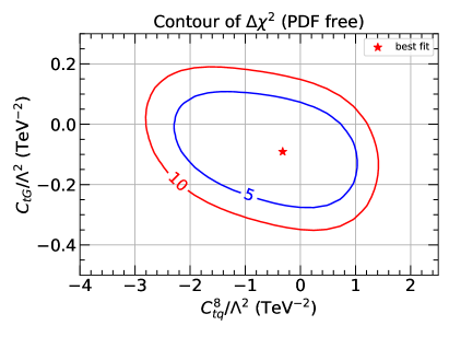
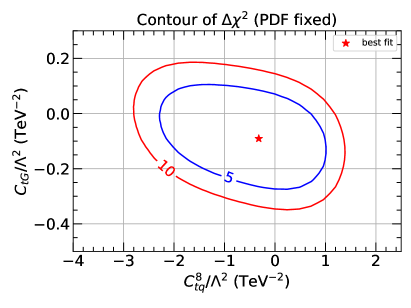
Figure 12: Contour plot of $\Delta\chi^{2}$ on the plane of $C_{tq}^{8}/\Lambda^{2}$ vs. $C_{tG}/\Lambda^{2}$ with the PDF parameters freely varying (left panel) or fixed to their best-fit values (right).

6 LM scans with jet production

Following the exploration of $t\bar{t}$ data and top-associated SMEFT operators in the section above, we now turn our attention to the determination of the Wilson coefficient $C_{1}$ from Eq. (2.1) via LM scans with a special focus on jet production measurements. In addition, we study the interplay between the Wilson coefficients primarily associated with jet production ($C_{1}$) and the top-associated Wilson coefficient most correlated with the gluon PDF ($C_{tG}$).

6.1 Contact interactions

For the additional studies shown below, we include 6 jet production data sets in our nominal fits as indicated in Tab. 3, including 3D distributions from the CMS 8 TeV dijet measurement and 2D distributions from the CMS 13 TeV inclusive jet measurement. In a variant fit, the CMS 8 TeV dijet data are replaced by corresponding data on inclusive jet production. Furthermore, we include all top-quark pair production experiments used in the nominal fits of Sec. 5 above as well as the other 32 baseline DIS/DY data sets, such the fits here represent the fullest accumulation of data considered in this work. We note, however, that these other experiments do not directly constrain the contact-interaction Wilson coefficient, $C_{1}$. In keeping with our nominal choices, the values of $\alpha_{s}(M_{Z})$ and $m_{t}$ are set to their respective world averages, $\alpha_{s}(M_{Z})=0.118$ and $m_{t}=172.5$ GeV. Also, contributions from the other Wilson coefficients associated with top production are not included here unless otherwise specified.

The results of the LM scans over $C_{1}$ according to our nominal setup are shown in Fig. 13, where the left panel shows the CMS 13 TeV inclusive jet data and CMS 8 TeV dijet data to have the tightest constraint, in addition to exhibiting a more subtle nonlinear dependence on $C_{1}/\Lambda^{2}$ as one moves away from the best fit. As in the previous section, the uncertainty range is mostly determined by the penalty term of these two leading data sets. In comparison, the sensitivity of the other jet data to $C_{1}$ is much weaker. Much as expected, there are almost no constraints from the data sets on top-quark pair production. The LM scans predict $C_{1}/\Lambda^{2}=-0.0015^{+0.0033}_{-0.0014}$ TeV^-2 at 90% CL, consistent with the SM. In the right panel, the PDF parameters are fixed to their values at the global minimum. We find that the behaviors of both global $\Delta\chi^{2}$ and individual $\Delta\chi^{2}$ are very similar to that shown in the left panel. The LM scans predict a result of $C_{1}/\Lambda^{2}=-0.0015^{+0.0024}_{-0.0014}$ TeV^-2 at 90% CL which has smaller uncertainties comparing with including PDF variations.

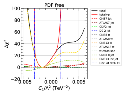
((a))

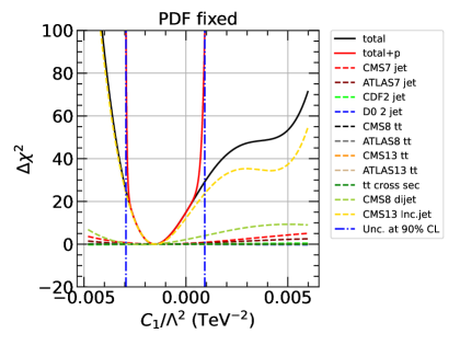
((b))

Figure 13: LM scans over $C_{1}/\Lambda^{2}$ in our nominal setup allowing the PDF parameters to freely float (left panel) or be fixed at the global minimum (right panel).

The total values of $\chi^{2}$, as well as those for individual jet data sets, are listed in Tab. 7 for the global minimum determined with and without the BSM SMEFT contributions. We find that the inclusion of SMEFT contributions causes the global $\chi^{2}$ to diminish by 13.7 units. Of this, the individual $\chi^{2}$ values for the CMS 8 TeV dijet data and 13 TeV inclusive jet data are reduced by 5.2 and 8.8 units, respectively, which is consistent with the left panel of Fig. 13. Meanwhile, the individual $\chi^{2}$ values of the other jet data sets are largely unaltered. Despite this apparent insensitivity, these experiments are important nonetheless for pinning down uncertainties in the gluon PDF and thus reducing correlations between the Wilson coefficient and PDFs in the global analyses. Notably, in the right panel of Fig. 13, we see evidence of somewhat more significant PDF-SMEFT correlations, a feature which can be deduced by comparing the dependence of the $\Delta\chi^{2}$ profiles on $C_{1}/\Lambda^{2}$; in particular, the size and shape of the $\Delta\chi^{2}$ curves for the CMS 8 TeV dijet and 13 TeV inclusive jet experiments are noticeably modified near $C_{1}/\Lambda^{2}\!\sim\!0.001\!$ TeV^-2 once PDF parameters are frozen in the right panel. These modifications lead to a moderate increase in the growth of $\Delta\chi^{2}$ at higher $C_{1}/\Lambda^{2}$ and a corresponding underestimate in the Wilson coefficient when not simultaneously fitted alongside the PDFs.

$\chi^{2}$ (nominal)	D0	CDF	ATLAS 7	CMS 7	CMS 8	CMS 13	global
$C_{1}=0$	112.91	113.35	198.90	203.95	184.15	119.55	4388.93
$C_{1}$ free	113.21	113.01	198.29	204.77	178.96	110.77	4375.23

Table 7: The total $\chi^{2}$ and the $\chi^{2}$ for individual jet experiments at the global minimum determined with and without SMEFT contributions parametrized by $C_{1}$.

It has been suggested 1101.4611 that contact interactions might be constrained by dijet or inclusive jet production. Apart from a modified energy dependence, contact interactions may also induce a different angular distribution in dijet production relative to purely SM predictions. To explore this point, we compare constraints from the CMS 8 TeV dijet and inclusive jet data directly. They are from the same data sample and differ only by the experimental observable. We perform LM scans on $C_{1}$ with the inclusion of either the CMS 8 TeV dijet or inclusive jet data respectively, meanwhile excluding the CMS 13 TeV inclusive jet data in the fit. The results of doing this are shown in Fig. 14. For the case of the CMS 8 TeV dijet data, in the left panel, we find that the CMS 8 TeV data together with the CMS and ATLAS 7 TeV jet data give the leading constraint. It predicts a result of $C_{1}/\Lambda^{2}=-0.0022^{+0.0187}_{-0.0054}$ TeV^-2 at 90% CL that has larger uncertainties than the result determined with our nominal setup, which is expected since the CMS 13 TeV jet data are not included here. In the right panel, we show the corresponding results for the CMS 8 TeV inclusive jet data. The LM scans predict $C_{1}/\Lambda^{2}=-0.0009^{+0.0138}_{-0.0045}$ TeV^-2 at 90% CL, that is, with reduced uncertainties relative to those determined from the CMS dijet data. By themselves, however, the CMS 8 TeV inclusive data prefer a larger value of $C_{1}/\Lambda^{2}\approx 0.008$ TeV^-2, with $\chi^{2}$ lowered by about 10 units relative to the global minimum.

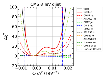
((a))

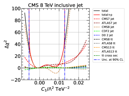
((b))

Figure 14: LM scans on $C_{1}/\Lambda^{2}$ with the inclusion of the CMS 8 TeV dijet data (left panel) or CMS 8 TeV inclusive jet data (right panel).

The results on the two CMS 8 TeV jet data are listed in Tab. 8. We also show the results from LM scans on $C_{1}$ with inclusion of only the CMS 13 TeV jet data for comparison. Note that, in all cases, the 7 TeV jet data, as well as the jet data from the Tevatron, are included in the fit. We further compare results obtained by fixing the PDF parameters to their values at the respective global minimum. The CMS 13 TeV jet data give the strongest constraint, more so than the two 8 TeV data, which is consistent with Fig. 13. Spuriously, the uncertainties on $C_{1}$ can be reduced significantly if the PDF parameters are fixed, as is seen, e.g., for the fit with CMS 13 TeV data alone.

TeV-2	nominal	CMS 8 dijet	CMS 8 jet	CMS 13 jet
PDF free	$-0.0015^{+0.0033}_{-0.0014}$	$-0.0022^{+0.0187}_{-0.0054}$	$-0.0009^{+0.0138}_{-0.0045}$	$-0.0013^{+0.0059}_{-0.0016}$
PDF fixed	$-0.0015^{+0.0024}_{-0.0014}$	$-0.0022^{+0.0180}_{-0.0051}$	$-0.0009^{+0.0131}_{-0.0049}$	$-0.0013^{+0.0026}_{-0.0015}$

Table 8: Constraints on $C_{1}/\Lambda^{2}$ in ${\rm TeV}^{-2}$ at 90% CL with individual data set on jet production.

In Fig. 15, we compare the gluon PDFs at $Q_{0}=1.295$ GeV determined by fitting with and without SMEFT. In the left panel, we find almost no change for $x<0.1$, and an upward shift smaller than 2% around $x\sim 0.3$, due to the active inclusion of SMEFT. In addition, a slight downward shift on both the central value and the uncertainty region can be found in the region of $x>0.5$. In the right panel, the relative PDF uncertainties are shown to slightly increase in the regions of $x\sim 0.25$ and $x\gtrsim 0.4$ for the combined PDF+SMEFT analysis. We conclude from Fig. 15 that $C_{1}$ is moderately correlated with the gluon PDF at large $x$.

((a))

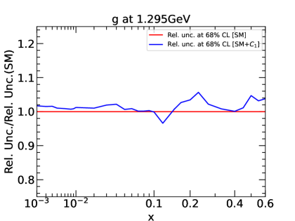
((b))

Figure 15: The gluon PDFs $g(x,Q)$, as determined by fitting with and without SMEFT contributions at $Q_{0}=1.295$ GeV, are shown in the left panel. The blue and red solid lines represent the central values determined by fitting with and without SMEFT contributions, respectively. The PDF uncertainties at 68% CL are indicated by hatched areas in the relevant colors. The relative uncertainties are shown in the right panel the same colors, normalized to the SM calculation.

6.2 Interplay with top-quark production

It is interesting and important to study the interplay between the Wilson coefficients relevant for jet production and those for top-quark pair production in the global analysis. It is reasonable to expect some level of correlations between these since both jet and top-quark pair production are ostensibly sensitive to the gluon PDF. In this subsection we test these possible correlations through simultaneous fits of PDFs, $C_{1}$, and $C_{tG}$. Specifically, we perform a series of LM scans on the individual coefficients by fixing either $C_{1}$, $C_{tG}$, or neither, with the fitted results for these coefficients summarized in Tab. 9. In the first column, both $C_{1}$ and $C_{tG}$ are free, whereas in the second and third columns, either $C_{1}$ or $C_{tG}$ is fixed to 0. We find that the best-fit value and uncertainty on both coefficients are practically unchanged when fixing either one coefficient or the other. This indicates no direct correlation between $C_{1}$ and $C_{tG}$, and is reinforced by the corresponding 2D LM scans in Fig. 16. In Fig. 16, which explicitly plots the 2D LM scans correlating $C_{1}$ and $C_{tG}$, the blue and red contours represent surfaces of constant $\Delta\chi^{2}=5$ and $10$, respectively. In the left panel, the very weak correlation between $C_{1}$ and $C_{tG}$ is realized in the robust rotational symmetry of the contour plot, especially in light of the fact that neither SMEFT coefficient exhibited particularly strong correlation with the gluon PDF in the studies shown above. In the right panel, the PDF parameters are fixed to their values at the global minimum. The contours are slightly smaller than those shown in the left panel, which indicates weak correlations between SMEFT and PDF parameters.

TeV-2	$C_{1}$, $C_{tG}$ free	fix $C_{1}$	fix $C_{tG}$
$C_{1}/\Lambda^{2}$	$-0.0015^{+0.0033}_{-0.0014}$	0	$-0.0015^{+0.0033}_{-0.0014}$
$C_{tG}/\Lambda^{2}$	$-0.120^{+0.248}_{-0.309}$	$-0.117^{+0.247}_{-0.309}$	0

Table 9: Constraints on $C_{1}/\Lambda^{2}$ and $C_{tG}/\Lambda^{2}$ at 90% CL from fits in which the SMEFT coefficients are fixed or allowed to freely vary.

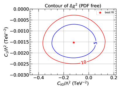
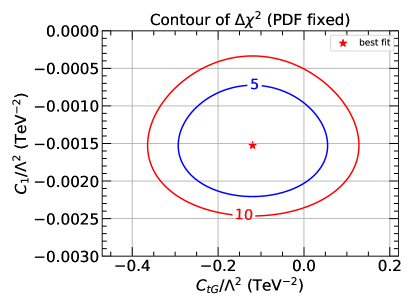
Figure 16: Contour plot of $\Delta\chi^{2}$ on the plane of $C_{tG}/\Lambda^{2}$ vs. $C_{1}/\Lambda^{2}$ with the PDF parameters freely varying (left panel) or fixed to their best-fit values (right).

In Fig. 17, we compare gluon PDFs at $Q_{0}=1.295$ GeV determined by fitting with and without SMEFT contributions from $O_{1}$ and $O_{tG}$. The impact on the gluon PDFs are mostly at large $x$. In the left panel, a slight upward shifts on both the central value and uncertainty region can be found in the region of $x\sim 0.3$ from SMEFT. A slight downward shift, smaller than 5%, on the central value can similarly be seen near $x\sim 0.6$. In the right panel, the relative uncertainties at 68% CL are shown, normalized for comparison as before. We find that relative uncertainties are slightly enhanced when fitting SMEFT for $x\sim 0.01$, $x\sim 0.2$, and $x\gtrsim 0.4$; while the $x$ dependence revealed in this case is somewhat different, these enhancements do not exceed in size those seen when fitting $C_{1}$ or $C_{tG}$ separately

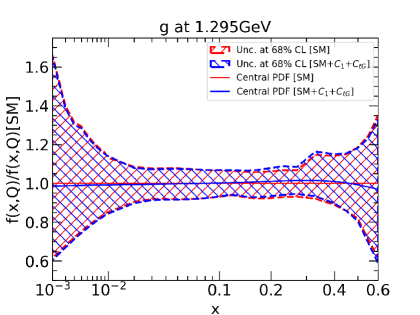
((a))

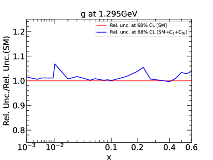
((b))

Figure 17: The gluon PDF determined by fitting with and without SMEFT contributions from both $O_{1}$ and $O_{tG}$ at $Q_{0}=1.295$ GeV is shown in the left panel. The blue and red solid lines represent the central values determined by fitting with and without SMEFT contributions, respectively. The PDF uncertainties at the 68% CL are shown via hatched areas in the corresponding colors. The relative uncertainties at 68% CL are shown in the right panel, normalized as in previous plots.

7 Discussion

Following the detailed presentation of the various combined PDF+SMEFT fits shown above, in the present section we briefly discuss a number topics which are particularly central to these joint fits and their interpretation. These issues include further discussion of correlations between the Wilson coefficients and PDFs (Sec. 7.1) as well as the question of any dependence on the assumed statistical procedure (Sec. 7.2), for which we present several comparisons.

7.1 Correlations between PDFs and SMEFT

Through the fitted PDFs and LM scans examined in the previous sections, we have seen evidence of mild correlations between the extracted SMEFT coefficients and PDFs in joint fits of these quantities. We observe PDF-SMEFT correlations as shifts in the PDF uncertainties once global fits are expanded to include freely-fitted SMEFT Wilson coefficients, such as the $C_{1}$ operator associated with contact interactions probed by jet production. Such correlations become more evident under scenarios in which the SMEFT coefficients deviate more significantly from the pure, $C\!=\!0$, SM context. This can be seen in the left panel of Fig. 18, in which we again plot the fitted gluon PDF, normalized to the SM CT18 NNLO baseline as in Fig. 15, but now including two additional fits in which $C_{1}$ is fixed at the extrema of its 90% uncertainty interval, resulting in the two additional dashed-black curves. While correlations remain relatively modest, it is noteworthy that the deviations of the fitted gluon from the purely SM PDF fits under these larger $C\!\neq\!0$ scenarios can rise to an appreciable fraction of the SM gluon PDF uncertainty, especially for $x\!\gtrsim\!0.1$ and above. It is reasonable to expect potentially significant correlations between, e.g., the gluon PDF and SMEFT coefficients, especially when these quantities are fitted to individual data sets, as both top-quark pair and jet production are generally thought to be sensitive to both. In a realistic global analysis, however, the gluon PDF is constrained by a diverse collection of experiments with unique pulls on the PDFs and their underlying $x$ dependence; these fitted experiments include a variety of data sets other than $t\bar{t}$ or jet production, such as DIS measured at high precision. Moreover, even among the jet measurements we include, there are distinct center-of-mass energies and various distributions in $y$, $p_{T}$, and $m_{t\bar{t}}$, each of which may differently probe the gluon PDF. These considerations have the effect of diluting the correlations between the PDF pulls of individual data sets and the preferences of the full fit for specific SMEFT coefficients. On the other hand, this point underscores the importance of extracting PDFs through a global analysis with data sets spanning a wide range of energies in various channels.

The statements above are made on the basis of our analysis of contemporary hadronic data; in principle, however, the mild correlations we find may grow in strength with greater experimental precision at the HL-LHC or other future experiments. We therefore explore this potential for enhanced correlations between PDFs and Wilson coefficients at future runs of the LHC. To maximize the likelihood of obtaining strong correlations, we take an extreme case of only keeping the most sensitive data among all the top-quark pair and jet production sets explored in this work. This corresponds to the total cross section measurements for top-quark pair production as well as the CMS 13 TeV measurement of inclusive jet production. For the former, we then perform LM scans on the Wilson coefficient $C_{tG}$ in global fits in which these $t\bar{t}$ data are overweighted by a multiplicative weight factor placed on their associated $\chi^{2}$; this overweighting is statistically equivalent to an overall reduction in the uncorrelated uncertainty of the $t\bar{t}$ cross sections, thereby mimicking future improvements in both experimental precision and theoretical accuracy. The final uncertainties on $C_{tG}$ are determined with the criterion $\Delta\chi^{2}=2.706$ for simplicity, under separate scenarios in which the PDFs are either frozen at their global minima or allowed to float freely. The ratio of the uncertainties on the SMEFT coefficients for the fits with fixed or free PDFs can be interpreted as an indication of the degree to which $C_{tG}$ might be correlated with the PDFs, which we trace as a function of total the precision of the $t\bar{t}$ data (i.e., the “Weight” on the data). We carry out identical scans on the Wilson coefficient $C_{1}$, in this case, placing the additional weight on the individual $\chi^{2}$ of the inclusive jet data, rather than the $t\bar{t}$.

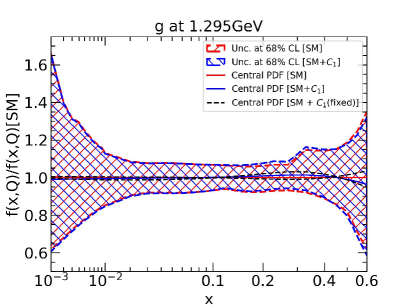
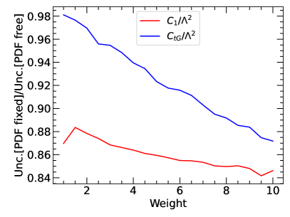
Figure 18: At left, we plot the gluon PDF ratio analogous to Fig. 15 (left), now including two additional fits (dashed-black) in which the $C_{1}$ SMEFT coefficient is fixed to the extremal values allowed within a 90% CL. In the right panel, we plot the ratio of the uncertainties determined with the PDF parameters fixed at the global minimum to the uncertainties determined with the PDF parameters free for $C_{1}/\Lambda^{2}$ and $C_{tG}/\Lambda^{2}$.

In Fig. 18 (right), we show the ratios described above as functions of the chosen Weight for both $C_{tG}$ and $C_{1}$. Specifically, the ratio starts at 0.98 (0.87) for $\mathrm{Weight}\!=\!1$, and decreases to approximately 0.87 (0.84) near $\mathrm{Weight}\!=\!10$ for $C_{tG}$ ($C_{1}$). We thus find that the uncertainty ratio for $C_{1}$ is always smaller than the corresponding ratio for $C_{tG}$, indicating stronger correlations with the fitted PDFs and a greater underestimate in the uncertainty for this SMEFT coefficient when PDFs are not simultaneously fitted; this is true for all Weights considered on these leading experiments. At the same time, it is noteworthy that the $\mathrm{Weight}\!=\!10$ overweighting of the $t\bar{t}$ data leads to a more rapid relative increase in the size of the PDF-SMEFT correlations than the corresponding shift found for $C_{1}$ and the jet data. We note that taking $\mathrm{Weight}\!=\!10$ may be interpreted in terms of a corresponding reduction in the total uncorrelated uncertainties for the fitted jet and $t\bar{t}$ experiments. Assuming the Weight to be an overall prefactor on the contribution to $\chi^{2}$ from a given experimental data set, $\mathrm{Weight}\!=\!10$ then corresponds to a reduction in the total uncorrelated (statistical and uncorrelated systematic) uncertainty by a factor of $\sqrt{10}\!\approx\!3$. For comparison, the optimistic-scenario PDF projections of Ref AbdulKhalek:2018rok assumed improvements by a factor of 2-3 in systematic uncertainties at HL-LHC as well as $\mathcal{L}\!=\!3\,\mathrm{ab}^{-1}$ data sets at ATLAS — more than an order-of-magnitude increase in aggregated statistics. Thus, the $\approx\!10\%$ under-estimate in $C_{tG}/\Lambda^{2}$ shown in Fig. 18 (right) for $\mathrm{Weight}\!\sim\!7$ reflects the enhanced correlations which might reasonably be expected at HL-LHC under optimistic performance scenarios. We conclude that the correlations between the PDFs and SMEFT coefficients become stronger with increasing precision as expected — a general observation that must inform future studies. These projections are based on extrapolations starting from these particular $t\bar{t}$ and inclusive jet data; future experiments with higher initial precision may steepen the trajectories shown in Fig. 18 as uncertainties shrink. These potential correlations can be further enhanced when using a realistic tolerance criterion, which can only be studied with actual data rather than estimated via this simplified reweighting procedure.

7.2 Impact of different tolerance criteria

In this study, uncertainties on the PDFs and Wilson coefficients were determined according to the same tolerance criterion (1) as in the CT18 global analyses, namely, with $\Delta\chi^{2}+P=100$ at the 90% CL. With this criterion, both the change in the global $\chi^{2}$ and disagreements among individual data sets were considered at the same time. In contrast, the MSTW 0901.0002 family of analyses employ a dynamical tolerance criterion (2) in determinations of both PDF and parametric QCD uncertainties. Though broadly similar, the use of dynamical tolerance somewhat differs from the CT18 criterion: namely, variation in the global $\chi^{2}$ is not included in the dynamical tolerance, which instead differently normalizes the $\chi^{2}$ values of individual data sets at the global minimum. We emphasize that it is important to introduce the tolerance factors for a global analysis with many different data sets in order to account for possible tensions among the fitted experiments. In experimental analyses using fewer data sets, the usual parameter-fitting criterion (3) is always used with uncertainties at the 90% CL determined by requiring $\Delta\chi^{2}=2.706$. We note that there is also the so-called PDF profiling method (4) to fit input parameters together with PDFs through a series of nuisance parameters 1810.03639 ; 1906.10127 using Hessian PDFs from the global analyses. This is approximately equivalent to performing a global fit with reduced weights for the data sets used in the original PDF sets, when combining with the criterion of $\Delta\chi^{2}=2.706$. We compare the extracted Wilson coefficients using the four (1-4) criteria noted above in Fig. 19. In the last scenario, the $\chi^{2}$ of data sets other than the top-quark pair (jet) production have been divided by a factor of 10, the average tolerance at 68% CL, when included into the global $\chi^{2}$ in the fit of Wilson coefficients associated with top-quark pair (jet) production.

In Fig. 19, we plot the central values and uncertainties at 90% CL for each of the various Wilson coefficients fitted in this study. It can be seen that the CT18 and MSTW criteria show comparable results on the uncertainty range, as similarly observed in Ref. 2203.05506 for PDF uncertainties. The uncertainties from the CT18 criterion can be either slightly larger or smaller than those governed by the MSTW criterion, depending on the Wilson coefficients considered. The uncertainties determined with the usual parameter-fitting criterion are smaller by about a factor of 2 in the case of the Wilson coefficients associated with top-quark pair production. For the extraction of the contact-interaction coefficient, $C_{1}$, the dependence of the uncertainty on the tolerance criterion is even larger, where the uncertainty from the parameter-fitting criterion is smaller by a factor of 5. The SM ($C_{1}=0$) is excluded already if using the uncertainty estimated from the parameter-fitting criterion indicating the failure of such a criterion in the global analyses with large number of data sets. Results using the criterion with reduced weights applied to the data sets with minimal sensitivity show almost no difference with respect to the ones without reweighting.

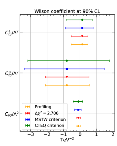
((a))

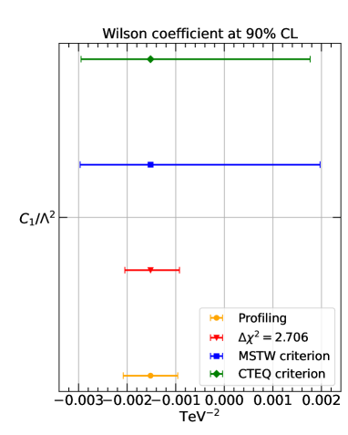
((b))

Figure 19: Constraints on the Wilson coefficients with different tolerance criteria. The marks and error bars respectively indicate the central values and uncertainties at 90% CL. The results with different tolerance criteria are shown with relevant colors.

Finally, we compare our results for the Wilson coefficients to those of previous studies. The ATLAS collaboration reports a 95% CL bound on $C_{tG}/\Lambda^{2}$ of [-0.52, 0.15] TeV^-2 using the transverse momentum distribution of the top quark measured at LHC 13 TeV in the hadronic decay channel with an integrated luminosity of 139 fb^-1 2202.12134 . Our nominal 90% CL bound is $[-0.40,0.16]$ TeV^-2, which is comparable with the ATLAS result. In addition, the ATLAS collaboration reports a 95% CL bound on $C_{tq}^{8}/\Lambda^{2}$ of [-0.64, 0.12] TeV^-2. Our nominal 90% CL bound is $[-3.2,1.8]$ TeV^-2, which is much weaker than the ATLAS result. There are two main reasons for this. First, we use the default CT18 tolerance rather than the parameter-fitting criterion. When using the criterion of $\Delta\chi^{2}=1.96^{2}$, we obtain a bound at 95% CL of [-2.28, 0.72] TeV^-2. Second, the ATLAS constraints are based on the transverse momentum distribution of the top quark. That in general leads to stronger constraints on the Wilson coefficient $C_{tq}^{8}/\Lambda^{2}$ than that found when using the $m_{t\bar{t}}$ distribution of the top-quark pair. For instance, in our study and the SMEFiT study of Ref. 2105.00006 , both of which use the $m_{t\bar{t}}$ distribution, the bounds on $C_{tq}^{8}/\Lambda^{2}$ are much weaker than the bounds on $C_{tG}/\Lambda^{2}$. Meanwhile in the ATLAS measurement, the bounds on $C_{tq}^{8}/\Lambda^{2}$ and $C_{tG}/\Lambda^{2}$ are comparable. In another analysis from CMS of inclusive jet production at 13 TeV (corresponding to the same data included in this work), a 95% CL result of $C_{1}/\Lambda^{2}\in[-0.0013,-0.0001]$ TeV^-2 was reported based on a joint fit of PDFs and contact interactions. In comparison, our nominal result of $[-0.0029,0.0018]$ TeV^-2 at the 90% CL is compatible considering the different criterion used.

8 Summary

SMEFT model-independently parametrizes BSM physics as might typically be formulated via phenomenological Lagrangians in the ultraviolet; this in turn provides a systematically-improvable framework for connecting BSM far above the electroweak scale to empirical consequences at lower energies — at the LHC or other facilities. Problematically, SMEFT-based BSM searches often involve the same collider data as those fitted in studies of proton PDFs, which are also core inputs to the SM theory predictions for BSM search baselines. To understand the extent to which this might introduce statistical bias into extractions of SMEFT coefficients, we perform a joint PDF+SMEFT fit based on an extension of the CT18 global analysis, and obtain a self-consistent determination of the possible BSM effects. The global analyses in this work are boosted with supervised machine learning techniques in the form of multi-layer perceptron neural networks to ensure efficient scans of the full PDF+SMEFT parameter space. To be specific, we compute $\chi^{2}$ profiles for all parameters, including the PDFs, strong coupling, $\alpha_{s}$, top-quark mass, $m_{t\bar{t}}$, and the SMEFT Wilson coefficients, finding these can be learned efficiently and with high fidelity by the neural network.

In this study, we focused on several SMEFT operators that are relevant for top-quark pair and jet production at hadron colliders. Regarding top-quark production, for the Wilson coefficients of the four-quark color-singlet and octet and gluonic operators, we obtain $C_{tu}^{1}/\Lambda^{2}=C_{td}^{1}/\Lambda^{2}=0.14^{+0.61}_{-0.97}$ TeV^-2, $C_{tq}^{8}/\Lambda^{2}=-0.80^{+2.58}_{-2.38}$ TeV^-2 and $C_{tG}/\Lambda^{2}=-0.10^{+0.26}_{-0.30}$ TeV^-2, respectively, at the 90% CL using the default CT tolerance. For jet production, we get $C_{1}/\Lambda^{2}=-0.0015^{+0.0033}_{-0.0014}$ TeV^-2 at 90% CL for the four-quark contact interactions. We find mild correlations between the extracted Wilson coefficients and PDFs, particularly, the gluon PDF at very high $x$, as well as other QCD parameters like the strong coupling and top-quark mass. While we investigated the effects of the combined PDF+SMEFT analyses on other PDF flavors, we generally found the impact in these cases to be much smaller than that observed for the gluon; simultaneous fits of additional SMEFT operators probed by other data sets may alter this picture, which we reserve for forthcoming studies. Though presently mild, we also find that these correlations between SMEFT coefficients and PDFs may grow significantly with higher precision in $t\bar{t}$ and jet production, as might be achievable at HL-LHC.

We have also examined the dependence of the Wilson coefficient uncertainties on the statistical criteria used in joint fits. We showed that, in the context of global analyses with a variety of experimental data, the CT18 and MSTW tolerance criteria result in similar uncertainties while the parameter-fitting and profiling criteria give much smaller uncertainties. This work serves as a new basis for joint analyses of SM and BSM in the setting of the CTEQ-TEA framework. In addition to being generalizable with additional machine-learning developments, this approach may also be regularly updated with new data from the LHC and other experiments, and a systematic study on SMEFT operators relevant for DY production and DIS processes is underway.

- (1) S. Weinberg, Phenomenological Lagrangians, Physica A 96 (1979), no. 1-2 327–340.
- (2) W. Buchmuller and D. Wyler, Effective Lagrangian Analysis of New Interactions and Flavor Conservation, Nucl. Phys. B 268 (1986) 621–653.
- (3) C. N. Leung, S. T. Love, and S. Rao, Low-Energy Manifestations of a New Interaction Scale: Operator Analysis, Z. Phys. C 31 (1986) 433.
- (4) ATLAS Collaboration, G. Aad et al., Determination of the parton distribution functions of the proton using diverse ATLAS data from collisions at , 8 and 13 TeV, Eur. Phys. J. C 82 (2022), no. 5 438, [arXiv:2112.11266].
- (5) D. Stump, J. Huston, J. Pumplin, W.-K. Tung, H. L. Lai, S. Kuhlmann, and J. F. Owens, Inclusive jet production, parton distributions, and the search for new physics, JHEP 10 (2003) 046, [hep-ph/0303013].
- (6) ZEUS Collaboration, H. Abramowicz et al., Limits on contact interactions and leptoquarks at HERA, Phys. Rev. D 99 (2019), no. 9 092006, [arXiv:1902.03048].
- (7) S. Carrazza, C. Degrande, S. Iranipour, J. Rojo, and M. Ubiali, Can New Physics hide inside the proton?, Phys. Rev. Lett. 123 (2019), no. 13 132001, [arXiv:1905.05215].
- (8) A. Greljo, S. Iranipour, Z. Kassabov, M. Madigan, J. Moore, J. Rojo, M. Ubiali, and C. Voisey, Parton distributions in the SMEFT from high-energy Drell-Yan tails, JHEP 07 (2021) 122, [arXiv:2104.02723].
- (9) M. Madigan and J. Moore, Parton Distributions in the SMEFT from high-energy Drell-Yan tails, PoS EPS-HEP2021 (2022) 424, [arXiv:2110.13204].
- (10) CMS Collaboration, A. Tumasyan et al., Measurement and QCD analysis of double-differential inclusive jet cross sections in proton-proton collisions at = 13 TeV, JHEP 02 (2022) 142, [arXiv:2111.10431].
- (11) S. Iranipour and M. Ubiali, A new generation of simultaneous fits to LHC data using deep learning, JHEP 05 (2022) 032, [arXiv:2201.07240].
- (12) S. Amoroso et al., Snowmass 2021 whitepaper: Proton structure at the precision frontier, arXiv:2203.13923.
- (13) J. Pumplin, D. R. Stump, and W. K. Tung, Multivariate fitting and the error matrix in global analysis of data, Phys. Rev. D 65 (2001) 014011, [hep-ph/0008191].
- (14) D. Stump, J. Pumplin, R. Brock, D. Casey, J. Huston, J. Kalk, H. L. Lai, and W. K. Tung, Uncertainties of predictions from parton distribution functions. 1. The Lagrange multiplier method, Phys. Rev. D 65 (2001) 014012, [hep-ph/0101051].
- (15) D. Liu, C. Sun, and J. Gao, Machine learning of log-likelihood functions in global analysis of parton distributions, arXiv:2201.06586.
- (16) T.-J. Hou et al., New CTEQ global analysis of quantum chromodynamics with high-precision data from the LHC, Phys. Rev. D 103 (2021), no. 1 014013, [arXiv:1912.10053].
- (17) G. Durieux, F. Maltoni, and C. Zhang, Global approach to top-quark flavor-changing interactions, Phys. Rev. D 91 (2015), no. 7 074017, [arXiv:1412.7166].
- (18) C. Degrande, F. Maltoni, J. Wang, and C. Zhang, Automatic computations at next-to-leading order in QCD for top-quark flavor-changing neutral processes, Phys. Rev. D 91 (2015) 034024, [arXiv:1412.5594].
- (19) D. Barducci et al., Interpreting top-quark LHC measurements in the standard-model effective field theory, arXiv:1802.07237.
- (20) N. P. Hartland, F. Maltoni, E. R. Nocera, J. Rojo, E. Slade, E. Vryonidou, and C. Zhang, A Monte Carlo global analysis of the Standard Model Effective Field Theory: the top quark sector, JHEP 04 (2019) 100, [arXiv:1901.05965].
- (21) I. Brivio, S. Bruggisser, F. Maltoni, R. Moutafis, T. Plehn, E. Vryonidou, S. Westhoff, and C. Zhang, O new physics, where art thou? A global search in the top sector, JHEP 02 (2020) 131, [arXiv:1910.03606].
- (22) C. Degrande, G. Durieux, F. Maltoni, K. Mimasu, E. Vryonidou, and C. Zhang, Automated one-loop computations in the standard model effective field theory, Phys. Rev. D 103 (2021), no. 9 096024, [arXiv:2008.11743].
- (23) E. Eichten, K. D. Lane, and M. E. Peskin, New Tests for Quark and Lepton Substructure, Phys. Rev. Lett. 50 (1983) 811–814.
- (24) E. Eichten, I. Hinchliffe, K. D. Lane, and C. Quigg, Super Collider Physics, Rev. Mod. Phys. 56 (1984) 579–707. [Addendum: Rev.Mod.Phys. 58, 1065–1073 (1986)].
- (25) P. Chiappetta and M. Perrottet, Possible bounds on compositeness from inclusive one jet production in large hadron colliders, Phys. Lett. B 253 (1991) 489–493.
- (26) O. Domenech, A. Pomarol, and J. Serra, Probing the SM with Dijets at the LHC, Phys. Rev. D 85 (2012) 074030, [arXiv:1201.6510].
- (27) J. Gao, C. S. Li, and C. P. Yuan, NLO QCD Corrections to dijet Production via Quark Contact Interactions, JHEP 07 (2012) 037, [arXiv:1204.4773].
- (28) M. Czakon and A. Mitov, Top++: A Program for the Calculation of the Top-Pair Cross-Section at Hadron Colliders, Comput. Phys. Commun. 185 (2014) 2930, [arXiv:1112.5675].
- (29) M. Czakon, P. Fiedler, and A. Mitov, Total Top-Quark Pair-Production Cross Section at Hadron Colliders Through , Phys. Rev. Lett. 110 (2013) 252004, [arXiv:1303.6254].
- (30) M. Czakon, D. Heymes, and A. Mitov, Dynamical scales for multi-TeV top-pair production at the LHC, JHEP 04 (2017) 071, [arXiv:1606.03350].
- (31) M. Czakon, D. Heymes, and A. Mitov, fastNLO tables for NNLO top-quark pair differential distributions, arXiv:1704.08551.
- (32) T. Kluge, K. Rabbertz, and M. Wobisch, FastNLO: Fast pQCD calculations for PDF fits, in 14th International Workshop on Deep Inelastic Scattering, pp. 483–486, 9, 2006. hep-ph/0609285.
- (33) fastNLO Collaboration, M. Wobisch, D. Britzger, T. Kluge, K. Rabbertz, and F. Stober, Theory-Data Comparisons for Jet Measurements in Hadron-Induced Processes, arXiv:1109.1310.
- (34) J. Alwall, R. Frederix, S. Frixione, V. Hirschi, F. Maltoni, O. Mattelaer, H. S. Shao, T. Stelzer, P. Torrielli, and M. Zaro, The automated computation of tree-level and next-to-leading order differential cross sections, and their matching to parton shower simulations, JHEP 07 (2014) 079, [arXiv:1405.0301].
- (35) M. Czakon, D. Heymes, A. Mitov, D. Pagani, I. Tsinikos, and M. Zaro, Top-pair production at the LHC through NNLO QCD and NLO EW, JHEP 10 (2017) 186, [arXiv:1705.04105].
- (36) K. Hagiwara, Y. Sumino, and H. Yokoya, Bound-state Effects on Top Quark Production at Hadron Colliders, Phys. Lett. B 666 (2008) 71–76, [arXiv:0804.1014].
- (37) Y. Kiyo, J. H. Kuhn, S. Moch, M. Steinhauser, and P. Uwer, Top-quark pair production near threshold at LHC, Eur. Phys. J. C 60 (2009) 375–386, [arXiv:0812.0919].
- (38) W.-L. Ju, G. Wang, X. Wang, X. Xu, Y. Xu, and L. L. Yang, Invariant-mass distribution of top-quark pairs and top-quark mass determination, Chin. Phys. C 44 (2020), no. 9 091001, [arXiv:1908.02179].
- (39) C. Schwan, N3pdf/pineappl: v0.5.2, Mar., 2022.
- (40) S. Carrazza, E. R. Nocera, C. Schwan, and M. Zaro, PineAPPL: combining EW and QCD corrections for fast evaluation of LHC processes, JHEP 12 (2020) 108, [arXiv:2008.12789].
- (41) J. Currie, E. W. N. Glover, and J. Pires, Next-to-Next-to Leading Order QCD Predictions for Single Jet Inclusive Production at the LHC, Phys. Rev. Lett. 118 (2017), no. 7 072002, [arXiv:1611.01460].
- (42) J. Currie, A. Gehrmann-De Ridder, T. Gehrmann, E. W. N. Glover, A. Huss, and J. a. Pires, Infrared sensitivity of single jet inclusive production at hadron colliders, JHEP 10 (2018) 155, [arXiv:1807.03692].
- (43) T. Gehrmann et al., Jet cross sections and transverse momentum distributions with NNLOJET, PoS RADCOR2017 (2018) 074, [arXiv:1801.06415].
- (44) Z. Nagy, Three jet cross-sections in hadron hadron collisions at next-to-leading order, Phys. Rev. Lett. 88 (2002) 122003, [hep-ph/0110315].
- (45) Z. Nagy, Next-to-leading order calculation of three jet observables in hadron hadron collision, Phys. Rev. D 68 (2003) 094002, [hep-ph/0307268].
- (46) S. Dittmaier, A. Huss, and C. Speckner, Weak radiative corrections to dijet production at hadron colliders, JHEP 11 (2012) 095, [arXiv:1210.0438].
- (47) J. Gao, C. S. Li, J. Wang, H. X. Zhu, and C. P. Yuan, Next-to-leading QCD effect to the quark compositeness search at the LHC, Phys. Rev. Lett. 106 (2011) 142001, [arXiv:1101.4611].
- (48) J. Gao, CIJET: A program for computation of jet cross sections induced by quark contact interactions at hadron colliders, Comput. Phys. Commun. 184 (2013) 2362–2366, [arXiv:1301.7263].
- (49) xFitter Collaboration, H. Abdolmaleki et al., xFitter: An Open Source QCD Analysis Framework. A resource and reference document for the Snowmass study, 6, 2022. arXiv:2206.12465.
- (50) J. Pumplin, D. R. Stump, J. Huston, H. L. Lai, P. M. Nadolsky, and W. K. Tung, New generation of parton distributions with uncertainties from global QCD analysis, JHEP 07 (2002) 012, [hep-ph/0201195].
- (51) R. D. Ball et al., Parton Distribution Benchmarking with LHC Data, JHEP 04 (2013) 125, [arXiv:1211.5142].
- (52) NNPDF Collaboration, R. D. Ball, L. Del Debbio, S. Forte, A. Guffanti, J. I. Latorre, J. Rojo, and M. Ubiali, Fitting Parton Distribution Data with Multiplicative Normalization Uncertainties, JHEP 05 (2010) 075, [arXiv:0912.2276].
- (53) J. Gao, L. Harland-Lang, and J. Rojo, The Structure of the Proton in the LHC Precision Era, Phys. Rept. 742 (2018) 1–121, [arXiv:1709.04922].
- (54) CDF, D0 Collaboration, T. A. Aaltonen et al., Combination of Measurements of the Top-Quark Pair Production Cross Section from the Tevatron Collider, Phys. Rev. D 89 (2014), no. 7 072001, [arXiv:1309.7570].
- (55) ATLAS Collaboration, G. Aad et al., Measurement of the production cross-section using events with b-tagged jets in pp collisions at = 7 and 8 with the ATLAS detector, Eur. Phys. J. C 74 (2014), no. 10 3109, [arXiv:1406.5375]. [Addendum: Eur.Phys.J.C 76, 642 (2016)].
- (56) CMS Collaboration, S. Chatrchyan et al., Measurement of the Production Cross Section in the Dilepton Channel in Collisions at TeV, JHEP 11 (2012) 067, [arXiv:1208.2671].
- (57) CMS Collaboration, V. Khachatryan et al., Measurement of the t-tbar production cross section in the e-mu channel in proton-proton collisions at sqrt(s) = 7 and 8 TeV, JHEP 08 (2016) 029, [arXiv:1603.02303].
- (58) ATLAS Collaboration, Measurement of the production cross-section and lepton differential distributions in dilepton events from collisions at TeV with the ATLAS detector, .
- (59) CMS Collaboration, V. Khachatryan et al., Measurement of the production cross section using events in the e final state in pp collisions at 13 TeV, Eur. Phys. J. C 77 (2017) 172, [arXiv:1611.04040].
- (60) ATLAS Collaboration, G. Aad et al., Measurements of top-quark pair differential cross-sections in the lepton+jets channel in collisions at TeV using the ATLAS detector, Eur. Phys. J. C 76 (2016), no. 10 538, [arXiv:1511.04716].
- (61) CMS Collaboration, A. M. Sirunyan et al., Measurement of double-differential cross sections for top quark pair production in pp collisions at TeV and impact on parton distribution functions, Eur. Phys. J. C 77 (2017), no. 7 459, [arXiv:1703.01630].
- (62) CMS Collaboration, V. Khachatryan et al., Measurement of the differential cross section for top quark pair production in pp collisions at , Eur. Phys. J. C 75 (2015), no. 11 542, [arXiv:1505.04480].
- (63) ATLAS Collaboration, G. Aad et al., Measurements of top-quark pair differential and double-differential cross-sections in the +jets channel with collisions at TeV using the ATLAS detector, Eur. Phys. J. C 79 (2019), no. 12 1028, [arXiv:1908.07305]. [Erratum: Eur.Phys.J.C 80, 1092 (2020)].
- (64) CMS Collaboration, A. M. Sirunyan et al., Measurements of differential cross sections in proton-proton collisions at 13 TeV using events containing two leptons, JHEP 02 (2019) 149, [arXiv:1811.06625].
- (65) CDF Collaboration, T. Aaltonen et al., Measurement of the Inclusive Jet Cross Section at the Fermilab Tevatron p anti-p Collider Using a Cone-Based Jet Algorithm, Phys. Rev. D 78 (2008) 052006, [arXiv:0807.2204]. [Erratum: Phys.Rev.D 79, 119902 (2009)].
- (66) D0 Collaboration, V. M. Abazov et al., Measurement of the inclusive jet cross-section in collisions at =1.96-TeV, Phys. Rev. Lett. 101 (2008) 062001, [arXiv:0802.2400].
- (67) ATLAS Collaboration, G. Aad et al., Measurement of the inclusive jet cross-section in proton-proton collisions at TeV using 4.5 fb -1 of data with the ATLAS detector, JHEP 02 (2015) 153, [arXiv:1410.8857]. [Erratum: JHEP 09, 141 (2015)].
- (68) CMS Collaboration, S. Chatrchyan et al., Measurement of the Ratio of Inclusive Jet Cross Sections using the Anti- Algorithm with Radius Parameters R=0.5 and 0.7 in pp Collisions at TeV, Phys. Rev. D 90 (2014), no. 7 072006, [arXiv:1406.0324].
- (69) CMS Collaboration, V. Khachatryan et al., Measurement and QCD analysis of double-differential inclusive jet cross sections in pp collisions at TeV and cross section ratios to 2.76 and 7 TeV, JHEP 03 (2017) 156, [arXiv:1609.05331].
- (70) CMS Collaboration, A. M. Sirunyan et al., Measurement of the triple-differential dijet cross section in proton-proton collisions at and constraints on parton distribution functions, Eur. Phys. J. C 77 (2017), no. 11 746, [arXiv:1705.02628].
- (71) M. Cacciari, G. P. Salam, and G. Soyez, The anti- jet clustering algorithm, JHEP 04 (2008) 063, [arXiv:0802.1189].
- (72) Particle Data Group Collaboration, R. Workman et al., Review of Particle Physics, . to be published (2022).
- (73) CMS Collaboration, A. M. Sirunyan et al., Measurement of normalised multi-differential cross sections in pp collisions at TeV, and simultaneous determination of the strong coupling strength, top quark pole mass, and parton distribution functions, Eur. Phys. J. C 80 (2020), no. 7 658, [arXiv:1904.05237].
- (74) SMEFiT Collaboration, J. J. Ethier, G. Magni, F. Maltoni, L. Mantani, E. R. Nocera, J. Rojo, E. Slade, E. Vryonidou, and C. Zhang, Combined SMEFT interpretation of Higgs, diboson, and top quark data from the LHC, JHEP 11 (2021) 089, [arXiv:2105.00006].
- (75) R. Gomez Ambrosio, J. ter Hoeve, M. Madigan, J. Rojo, and V. Sanz, Unbinned multivariate observables for global SMEFT analyses from machine learning, arXiv:2211.02058.
- (76) R. Abdul Khalek, S. Bailey, J. Gao, L. Harland-Lang, and J. Rojo, Towards Ultimate Parton Distributions at the High-Luminosity LHC, Eur. Phys. J. C 78 (2018), no. 11 962, [arXiv:1810.03639].
- (77) A. D. Martin, W. J. Stirling, R. S. Thorne, and G. Watt, Parton distributions for the LHC, Eur. Phys. J. C 63 (2009) 189–285, [arXiv:0901.0002].
- (78) R. Abdul Khalek, S. Bailey, J. Gao, L. Harland-Lang, and J. Rojo, Towards Ultimate Parton Distributions at the High-Luminosity LHC, Eur. Phys. J. C 78 (2018), no. 11 962, [arXiv:1810.03639].
- (79) R. Abdul Khalek, S. Bailey, J. Gao, L. Harland-Lang, and J. Rojo, Probing Proton Structure at the Large Hadron electron Collider, SciPost Phys. 7 (2019), no. 4 051, [arXiv:1906.10127].
- (80) R. D. Ball et al., The PDF4LHC21 combination of global PDF fits for the LHC Run III, arXiv:2203.05506.
- (81) ATLAS Collaboration, G. Aad et al., Measurements of differential cross-sections in top-quark pair events with a high transverse momentum top quark and limits on beyond the Standard Model contributions to top-quark pair production with the ATLAS detector at = 13 TeV, JHEP 06 (2022) 063, [arXiv:2202.12134].