A group from a map and orbit equivalence.

Abstract

In two papers published in 1979, R. Bowen and C. Series defined a dynamical system from a Fuchsian group, acting on the hyperbolic plane $\mathbb{H}^{2}$. The dynamics is given by a map on $S^{1}$ which is, in particular, an expanding piecewise homeomorphism of the circle. In this paper we consider a reverse question: which dynamical conditions for an expanding piecewise homeomorphism of $S^{1}$ are sufficient for the map to be a “Bowen-Series-type” map (see below) for some group $G$ and which groups can occur? We give a partial answer to these questions.

1 Introduction

In this paper we introduce a class of discontinuous expanding piecewise homeomorphisms of the circle. Such a map $\Phi:S^{1}\rightarrow S^{1}$ is given by a finite partition of the circle so that the restriction of $\Phi$ to each partition interval is an expanding homeomorphism onto its image. The class of maps we consider is motivated by two related questions:
- Can we construct a group $G_{\Phi}$ from such a map $\Phi$?
- Which groups can be obtained?

The groups that can possibly be constructed are naturally subgroups of $\textrm{Homeo}(S^{1})$ which is well known for having many different classes of subgroups. Since the possible groups $G_{\Phi}$ and the map $\Phi$ act on the same space, $S^{1}$, it is natural to compare the two actions and the best possible situation is when the two actions are “orbit equivalent”. This means that the orbits of $\Phi$ and of $G_{\Phi}$ are the same, modulo possibly finitely many exceptions. In such cases we say that the map $\Phi$ is a Bowen-Series-type map for the group $G_{\Phi}$.

This program is a reverse problem of a beautiful construction initiated by R. Bowen and C. Series in the late 70’s in [B] and [BS], where they discovered a striking relationship between some groups and some dynamics. The Bowen-Series construction starts with a Fuchsian group $G$ given by an action on $\mathbb{H}^{2}$ with specific properties and they obtained a particular map $\Phi_{BS}:S^{1}\rightarrow S^{1}$, where $S^{1}$ is the boundary $\partial\mathbb{H}^{2}$. Some variations of this construction has been studied by Adler-Flato in [AF] and more recently in [AKM]. The maps $\Phi_{BS}$ satisfy very strong properties:
- They are piecewise Möbius maps,
- orbit equivalent to the $G$-action on $S^{1}$,
- expanding Markov maps.

The idea of the Bowen-Series construction has been revisited in [L] for hyperbolic surface groups, in the geometric group theory context, i.e. the group is given combinatorially by a presentation $P=\langle X;R\rangle$, i.e. a set of generators and relations. The presentations belong to a particular class called “geometric”, meaning that the associated Cayley 2-complex is planar. The classical presentations of surface groups are geometric in this sense as well as the presentations obtained from [AF]. This construction starts with a geometric presentation $P$ and defines a map $\Phi_{P}:S^{1}\rightarrow S^{1}$ that is an expanging piecewise homeomorphism and the circle is the Gromov boundary of the group $G$ (see [Gr]). The maps $\Phi_{P}$ and $\Phi_{BS}$ are different, i.e non conjugated, even in the cases they can be compared, i.e. for the classical presentations. But they satisfy the same two main features: the orbit equivalence and the Markov properties. The map $\Phi_{P}$ satisfies an additional property relating the group and the dynamics: the volume entropy of the presentation $P$ (see [GH]) equals the topological entropy of $\Phi_{P}$(see [AKM]). The construction of more maps from a geometric presentation $P$ of a surface group has been generalized in [AJLM2] by defining a multiparameter family of maps and an entropy stability result has been obtained for all maps in this familly.

The problem we consider in this paper is a converse question:
How particular are the maps obtained from a surface group presentation among piecewise homeomorphisms of the circle?
We obtain a partial answer to this general question. Here a map is given as a piecewise homeomorphism of the circle $\Phi$ and one goal is to find dynamical conditions on $\Phi$ that allow first to construct a group from the map and then to analyse which groups could be obtained. Each map $\Phi$, being a piecewise homeomorphisms of the circle, is given by a finite partition of $S^{1}$. It will soon becomes clear that the number of partition intervals has to be even. A point at the boundary of two partition intervals is called a cutting point, at such points the map is not continuous. The map is expanding means that each partition interval is mapped onto an interval that contains it compactly thus the map is surjective and not globally injective.

This class of maps is thus very different from the well known class of piecewise homeomorphisms, the classical “interval exchange transformations” (see W. Veech [V] and H. Masur [M] for instance) that are piecewise isometries.

The conditions we found on the map $\Phi$ are explained in §2, they can be expressed roughly as:

$\bullet$ A Strong Expansivity condition (SE): each partition interval is mapped to an interval that contains it and intersects all but one partition interval.

$\bullet$ An Eventual Coincidence condition (EC): the left and right orbits of each cutting point coincide after some well defined iterate.

$\bullet$ The conditions (E+) and (E-) that control the left and right orbits of the cutting points before the coincidence.

Finally we do not restrict to maps $\Phi$ satisfying a Markov property, as in [BS], [AF], [L], [AJLM], which would be too restrictive. We replace it by a weaker condition which quantifies the expansivity property:

$\bullet$ The Constant Slope conditions (CS): the map is conjugate to a piecewise affine map with constant slope ($\lambda>1$). Under this set of conditions our main result is:

Theorem.

Let $\Phi:S^{1}\rightarrow S^{1}$ be a piecewise orientation preserving homeomorphism satisfying the conditions: $\rm(SE),(EC),(E+),(E-),(CS)$. Then there exists a discrete subgroup $G_{\Phi}$ of ${\rm Homeo}^{+}(S^{1})$ such that:

1. $G_{\Phi}$ and $\Phi$ are orbit equivalent.

2. $G_{\Phi}$ is a surface group, for an orientable compact closed hyperbolic surface.

The set of maps satisfying the above conditions is not empty. Indeed if a surface group for an orientable surface has a geometric presentation $P$ where all the relations have even length (for instance the classical presentation) then the map $\Phi_{P}$ of [L] satisfies the conditions of the Theorem. For the same set of presentations the multiparameter family $\Phi_{\Theta}$ defined in [AJLM2] satisfies the conditions of the Theorem for an open set of parameters (see Lemma 1). On an other hand the set of conditions of the Theorem is not optimal (see Remark 1).

The strategy of proof has several steps. The first one is to analyse the dynamical properties of the map $\Phi$ (see §2 and §3). Then we construct a group $G_{X_{\Phi}}$, as a subgroup of ${\rm Homeo}^{+}(S^{1})$, by producing a generating set $X_{\Phi}$ from the map $\Phi$ (see §3). This step exhibits many choices for the generating set $X_{\Phi}$ and is more delicate than it first appears.

The next step is to prove that the group $G_{X_{\Phi}}$, as an abstract group, is hyperbolic in the sense of M. Gromov (see [Gr] or [GdlH]) and does not depend on the choices of the generating sets $X_{\Phi}$. This is obtained by showing that $G_{X_{\Phi}}$ acts geometrically on a hyperbolic metric space. This step is technical (see §4 and §5). It requires to construct a hyperbolic space and a geometric action on it from the only data we have: the map.

The hyperbolic space is obtained by a general dynamical construction inspired by one due to P. Haissinsky and K. Pilgrim [HP] (see §4). The hyperbolicity is a consequence of the expansivity, as in [HP], and the boundary of the space is $S^{1}$. We adapt the construction and define a new space, suited to the maps $\Phi$, specially the condition (EC), in order to define a group action on the space.

This step is new, it defines a class of “dynamical spaces” in the context of groups. The construction of an action of the group on this metric space is also new. In both cases, the space and the action are defined only from the dynamics of the map (see §5).

At this point the group $G_{\Phi}$ is hyperbolic with boundary $S^{1}$ and does not depend on the particular choices of the generators $X_{\Phi}$. A result of E. Freden [F] implies that the group is a discrete convergence group, as defined by F. Gehring and G.Martin [GM] and thus it satisfies the conditions of the geometrisation theorem of P. Tukia [T], D. Gabai [G] and A. Casson-D. Jungreis [CJ]. The conclusion is that $G_{\Phi}$ is virtually a Fuchsian group. One more step shows that, with our assumptions, $G_{\Phi}$ is torsion free and, by H. Zieschang [Zi], it is a surface group.

Proving that the group $G_{\Phi}$ and the map $\Phi$ are orbit equivalent follows a similar strategy as in [BS] (see §6).

In the appendix (see §7), we give a direct proof that $G_{\Phi}$ is a surface group, without using the geometrisation theorems of Tukia, Gabai and Casson-Jungreis. All the hard work has, in fact, been done before: the geometric action constructed in §5 is extended to a free, co-compact action on a 2-disc.

With the results of this paper we obtain a partial answer to our general question. The conditions (E+) and (E-) are not optimal (see Remark 1) and finding better conditions is a challenge for futur works. The construction of the group from the map has revealed some surprises. For instance obtaining group relations, as in Theorem 1, show how delicate it is for a set of generators to verify some relations. This is specially difficult with our assumptions giving, at best, diffeomorphisms of classe $C^{1}$. The construction also indicates that groups that are not surface groups could possibly appear with different choices in the constructions. Which groups could possibly appear in our construction is an interesting question. Another surprise is the relationship between the length of an element, for the specific generators constructed in §3, with the growth property of that element (see Proposition 11 and Corollary 4).

The condition (EC) is central in our approach, it seems to be a new dynamical condition and is interesting in its own right. The class of discontinuous maps satisfying a condition (EC) is much larger than the one studied here.

The relationship between the growth properties of the map and of the group has not been considered in this paper. The work in [AJLM2] goes in that direction for all maps obtained from a geometric presentation. From that result, it turns out that the numbers $\lambda>1$ appearing in the condition (CS) are limited, they are algebraic integers. This property is satisfied for our maps satisfying the conditions (EC) and ($\textrm{E}_{\pm}$). In addition the logarithm of that number is the topological entropy of the map and is equal to the volume entropy of the obtained presentation of the group (see Corollary 3).

Aknowledgements: This work was partially supported by FAPESP (2016/24707-4). We thanks the hospitality of our research institutes: I2M in Marseille and DM-UFSCar in São Carlos, Brazil. We thanks the French-Uruguayan laboratory (IFUMI) in Montevideo where this work has been completed. The authors would like to thank P. Haissinsky and M. Boileau for their interest in this work and some comments on an earlier versions of the paper. We would like to thank the anonymous referee of a previous version who pointed out a gap in one argument. Closing this gap has proved to be very interesting, for this work and possibly others.

2 A class of piecewise homeomorphisms on $S^{1}$

We define in this section the class of maps that will be considered throughout the paper.
A map $\Phi:S^{1}\rightarrow S^{1}$ is a piecewise orientation preserving homeomorphism of the circle if there is a finite partition of $S^{1}$:

$$S^{1}=\bigcup_{j=1}^{M}I_{j}\textrm{, where each }I_{j}\textrm{ is half open,}$$ (1)

so that and $\Phi_{j}:=\Phi_{|_{I_{j}}}$ is an orientation preserving homeomorphism onto its image and each $I_{j}$ is maximal. We require further that the number of partition intervals is even: $M=2N$.

2.1 The class of maps

To state the next properties of the maps in our class, we introduce some notations.
Let $\zeta,\iota,\delta,\gamma$ be permutations of $\{1,\dots,2N\}$, such that:

• $\zeta$ is a cyclic permutation of order $2N$,

• $\iota$ is a fixed point free involution, i.e. for all $j\in\{1,\dots,2N\}$, $\iota(j)\neq j$ and $\iota^{2}=\textrm{id}$,
  such that: $\iota(j)\neq\zeta^{\pm 1}(j),\forall j\in\{1,\dots,2N\}$.
  This implies that $N>1$ and, to avoid special cases, we assume for the rest of the paper, that $N\geq 4$.

• From the permutations $\zeta$ and $\iota$ we define: $\gamma:=\zeta^{-1}\iota$ and $\delta:=\zeta\;\iota$.

Geometrically $\zeta$ is the permutation that realizes the adjacency permutation of the intervals $\{I_{1},\dots,I_{{2N}}\}$ along a given positive orientation of $S^{1}$. By convention $I_{{\zeta(j)}}$ is the interval that is adjacent to $I_{j}$ in the positive direction.
The interval $I_{{\iota(j)}}$ is an interval that is not $I_{j}$ and is not adjacent to $I_{j}$. The two intervals $I_{{\gamma(j)}}$ and $I_{{\delta(j)}}$ are the intervals adjacent to $I{{}_{\iota(j)}}$ (see Figure 1).

From now on we assume that all the cycles of $\gamma$ (and $\delta$ see Lemma 2 bellow), in its cycle decomposition, have a length $\ell[j]$ even and larger than $4$, i.e:

$$\ell[j]\textrm{ is even and }k(j)=\ell[j]/2\geq 2\textrm{, for all }j\in\{1,\dots,2N\}.$$ (2)

The map $\Phi:S^{1}\rightarrow S^{1}$ satisfies the following set of conditions.
Using the permutations above, $\Phi$ satisfies the Strong Expansivity condition if:
(SE)

$\forall j\in\{1,\dots,2N\}$, $\Phi(I_{j})\bigcap I_{k}=\emptyset\Leftrightarrow k=\iota(j)$, (see Figure 1).

This condition has some immediate consequences:
(I) $\Phi(I_{j})\bigcap I_{k}=I_{k}$, $\forall k\neq\iota(j),\gamma(j),\delta(j)$,
(II) The map $\Phi$ has an expanding fixed point in the interior of each $I_{j}$.
This is immediate from the definition of $\iota$ and (I), since $I_{j}\subset\Phi(I_{j})$.
(III) The map is surjective, non injective and each point $z\in S^{1}$ has $2N-1$ or $2N-2$ pre-images.

To fix the notations we write each interval $I_{j}:=[z_{j},z_{\zeta(j)})$, the points $z_{j}\in S^{1}$ are called the cutting points of $\Phi$. The map $\Phi$ is not continuous at each $z_{j}$.

Figure 1: Condition (SE)

The next condition makes the map $\Phi$ really particular, it is called the Eventual Coincidence condition:
(EC)      $\forall j\in\{1,\dots,2N\}$ and $\forall n\geq k(j)-1$, where $k(j)\geq 2$ is given by (2):

$\Phi^{n}(\Phi_{\zeta^{-1}(j)}(z_{j}))=\Phi^{n}(\Phi_{j}(z_{j})).$

In other words, each cutting point has a priori two different orbits, one from the positive side and one from the negative side of the point. The condition (EC) says that after $k(j)$ iterates these two orbits coincide. By (1) each $I_{j}:=[z_{j},z_{\zeta(j)})$ is half open, the notation $\Phi_{\zeta^{-1}(j)}(z_{j})$ is well defined by continuity on the left of $z_{j}$ of $\Phi_{\zeta^{-1}(j)}$.

The next set of conditions on the map gives some control on the first $k(j)-1$ iterates of the cutting points $z_{j}$, namely: For all $j\in\{1,\dots,2N\}$ and all $0\leq m\leq k(j)-2$:
(E+)

$\Phi^{m}(\Phi_{j}(z_{j}))\in I_{{}_{\delta^{m+1}(j)}}$,

(E-)

$\Phi^{m}(\Phi_{\zeta^{-1}(j)}(z_{j}))\in I_{{}_{\gamma^{m+1}(\zeta^{-1}(j))}}$.

These two conditions are interpreted as follows:
Consider (E+), for $m=0$ this is condition (SE) since $\Phi_{j}(z_{j})\in I_{\delta(j)}$, (see Figure 1). Then $\Phi_{j}(z_{j})$ is near the cutting point $z_{\delta(j)}$ in $I_{\delta(j)}$, since $\Phi(\Phi_{j}(z_{j}))\in I_{\delta^{2}(j)}$ (by $m=1$) and $I_{\delta^{2}(j)}$ is the interval containing $\Phi_{\delta(j)}(z_{\delta(j)})$ (by $m=0$ for $z_{\delta(j)}$ ) and so on up to $m=k(j)-2$.

The last condition quantifies the expansivity property of the map. It is not absolutely necessary but simplifies many arguments, it is called the Constant Slope condition:

(CS) $\Phi$ is topologically conjugate to a piecewise affine map $\tilde{\Phi}$ with constant slope $\lambda>1$.

The following result is a combination of several statements in [AJLM2] (see Theorem A and Lemma 5.1). It implies that the set of piecewise homeomorphisms of the circle satisfying the conditions (SE), (EC), (E-), (E+), (CS) is non empty.

Lemma 1.

Let $S$ be a closed compact orientable surface of negative Euler characteristic, and let $P=<X,R>$ be a geometric presentation of the fundamental group $G=\pi_{1}(S)$ (see [L]) so that all the relations in $R$ have even length. Then, in the Bowen-Series like family of maps $\Phi_{P,\Theta}$ defined in [AJLM2], there is an open set of parameters $\Theta$ so that the corresponding maps satisfies the conditions (SE), (EC), (E-), (E+),(CS). The parameters $\Theta$ belong to a product of $2N$ intervals, where 2N is the number of generators. In particular, for the same set of presentations the map $\Phi_{P}$ defined in [L] satisfy these properties.

Remark 1.

By the previous result the set of piecewise orientation preserving homeomorphisms satisfying the conditions (SE), (EC), (E+), (E-), (CS) is non empty and there is a familly of such maps for each orientable surface and each geometric presentation with even length relations. For the maps $\Phi_{P}$ constructed in [L] the proof of these properties is a direct check. In particular the constant slope condition (CS) is obtained using the Markov property satisfied by $\Phi_{P}$ via a standard Perron-Frobenius argument. In the more general cases of the family $\Phi_{P,\Theta}$ defined in [AJLM2], the constant slope condition is one statement of the main theorem of that paper.

If the presentation $P$ of the surface group $G$ is geometric and has some relations with odd length then the constructions in [L] apply but not those in [B] and [BS]. For these presentations, some conditions similar but different to (E+) and (E-) are satisfied. When the presentation $P$ has some relations of length 3, a condition weaker than (SE) is satisfied (see Lemma 5.2 in [L]). In all these cases the condition (CS) is satisfied and a condition similar to (EC) is satisfied fo some integers $k$. The condition (EC) is crutial in this paper and is not satisfied by all possible maps constructed via the general Bowen-Series-like strategy as in [AJLM2]. In particular it is not satisfied by the original map in [BS]. The set of conditions considered in this paper is thus non optimal to obtain a complete answer to our general question.

2.2 Elementary properties of the permutations $\delta$ and $\gamma$

The combinatorics of our class of maps is mainly encoded via the permutations $\delta$ and $\gamma$. For the rest of the work we need to understand, in particular, the cycle structure of these permutations. These cycles will appear everywhere. In this paragraph we point out some elementary properties of these permutations.

Lemma 2.

The permutations $\gamma$ and $\delta$ are conjugated, more precisely $\gamma=\iota^{-1}\delta^{-1}\iota.$

Proof.

Since $\delta$ and $\delta^{-1}$ are conjugated and $\iota^{-1}\delta^{-1}\iota=\iota(\iota\zeta^{-1})\iota=\zeta^{-1}\iota=\gamma,$ then $\delta$ and $\gamma$ are conjugated. ∎

To simplify the notations we will sometimes use: $\overline{j}:=\iota(j)$.

The two permutations $\gamma$ and $\delta$ have the same cycle structure. We obtain $\gamma$ from $\delta^{-1}$ by changing $j$ to $\overline{j}$ on its cycles. The cycle of $\gamma$ that contains $\overline{j}$ and the cycle of $\delta$ that contains $j$ have the same length. We denote this number by $\ell[j]$.

Lemma 3.

The integers $\zeta^{-1}(j)$, $\overline{j}$ and $\overline{\delta^{m-1}(j)}$ belong to the same cycle of $\gamma$ of length $\ell[j]$, for all $j\in\{1,\dots,2N\}$ and $0<m\leq\ell[j]$.

Proof.

From the definitions of $\iota,\;\gamma,\;\delta$ and Lemma 2, we have: $\gamma(\overline{j})=\zeta^{-1}\iota(\iota(j))=\zeta^{-1}(j)$ and $\overline{\delta^{m-1}(j)}=\iota(\delta^{m}\delta^{-1}(j))=(\iota\delta^{m}\iota^{-1})\zeta^{-1}(j)=\gamma^{-m}(\zeta^{-1}(j)).$ ∎

Lemma 4.

If $1\leq m\leq\ell[\overline{j}],$ then $\zeta(\gamma^{m}(j))=\overline{\gamma^{m-1}(j)}$. In particular if $\ell[\overline{j}]$ is even and $k(\overline{j})=\ell[\overline{j}]/2$ then $\zeta(\overline{\delta^{k(\overline{j})-1}\zeta(j)})=\overline{\gamma^{k(\overline{j})-1}(j)}.$

Proof.

Notice that $\zeta(\gamma^{m}(j))=\zeta\gamma(\gamma^{m-1}(j))=\zeta(\zeta^{-1}\iota)(\gamma^{m-1}(j))=\overline{\gamma^{m-1}(j)}$, and suppose that $\ell[\overline{j}]$ is even and let $k(\overline{j})=\ell[\overline{j}]/2$. From the first part of this Lemma, to obtain $\zeta(\overline{\delta^{k(\overline{j})-1}\zeta(j)})=\overline{\gamma^{k(\overline{j})-1}(j)}$, it is enough to show that $\overline{\delta^{k(\overline{j})-1}\zeta(j)}=\gamma^{k(\overline{j})}(j)$. In fact, by Lemma 2 and the definition of $\delta$ we have: $\gamma^{k(\overline{j})}(j)=\iota^{-1}\delta^{-k(\overline{j})}\iota(j)=\overline{\delta^{k(\overline{j})}\iota(j)}=\overline{\delta^{k(\overline{j})-1}\delta\iota(j)}=\overline{\delta^{k(\overline{j})-1}\zeta(j)}$. ∎

Lemma 5.

$\gamma(\overline{\delta^{m}(j)})=\overline{\delta^{m-1}(j)}$ and $\delta(\overline{\gamma^{m}(\zeta^{-1}(j))})=\overline{\gamma^{m-1}(\zeta^{-1}(j))}$, for $m=1,\dots,\ell[\overline{j}]$.

Proof.

In fact, by Lemma 4 and $\iota,\gamma,\delta$, we have: $\gamma(\overline{\delta^{m}(j)})=\zeta^{-1}\iota(\iota\delta^{m}(j))=\zeta^{-1}\delta(\delta^{m-1}(j))=\zeta^{-1}\zeta(\overline{\delta^{m-1}(j)})=\overline{\delta^{m-1}(j)},$ $\textrm{and }\;\delta(\overline{\gamma^{m}(\zeta^{-1}(j))})=\zeta\iota(\iota\gamma^{m}(\zeta^{-1}(j)))=\zeta\gamma(\gamma^{m-1}(\zeta^{-1}(j)))=\overline{\gamma^{m-1}(\zeta^{-1}(j)))}.$ ∎

3 Construction of a group from the map $\Phi$

In this section we construct a familly of subgroups of ${\rm Diffeo}^{+}(S^{1})$, from any map $\Phi$ in the class defined in §2.1, with $2N$ partition intervals. The diffeomorphisms we can construct with our assumptions, in particular the condition (CS), are of class $C^{1}$. The strategy is to define a set of $N$ elements in ${\rm Diffeo}^{+}(S^{1})$ using the particular properties of the map $\Phi$ and then we consider the group generated by this specific set of diffeomorphisms. The construction is highly non unique and one goal is to make the choices as explicit as possible. The first step is a “toy model” construction which is essencially a connect-the-dot argument for a set of $N$ diffeomorphisms constructed from $\Phi$. In the next step we use the conditions (EC), (E+), (E-) in a crucial way. Each diffeomorphism obtained in the first step is replaced by a parametrized familly. The new set of diffeomorphisms satisfy some “partial” equalities among specific compositions of the diffeomorphisms, imposed by the map $\Phi$ via the conditions (EC) and (E+), (E-) for each cutting point. The partial equalities, i.e. equalities restricted to an open set, are candidates to become some relations in ${\rm Diffeo}^{+}(S^{1})$, i.e. global equalities among some compositions. Observe that if we were working with analytic diffeomorphisms then a local equality would impose a global one. But we can only work in the class $C^{1}$ and thus obtaining a global equality from a local one requires much more work. The next step is a delicate “tuning” of the diffeomorphims within the families above. The idea is to adjust the parameters introduced in the previous step, in order that each partial equality becomes global, defining the expected set of relations in ${\rm Diffeo}^{+}(S^{1})$. The set of elements in ${\rm Diffeo}^{+}(S^{1})$ obtained in this section is used as a set of generators for an, a priori, familly of groups (see Theorem 1). This family of groups is the main object studied in the remaining parts of the paper. The parameters in the families above are rather explicit from the various choices made during the construction. One of the goal in the remaining parts of the paper will be to check that the abstract groups obtained do not really depend on these choices.

3.1 A toy model construction of diffeomorphisms from $\Phi$

By condition (CS) we replace our initial piecewise homeomorphism $\Phi$ by the piecewise affine map $\widetilde{\Phi}$ with constant slope $\lambda>1$, where $\widetilde{\Phi}=g^{-1}\circ\Phi\circ g$, for $g\in\textrm{Homeo}^{+}(S^{1})$. The piecewise affine map $\widetilde{\Phi}$ is defined by a partition: $S^{1}=\bigcup_{j=1}^{2N}\widetilde{I}_{j}$, where:

$\widetilde{I}_{j}=[\tilde{z}_{j},\tilde{z}_{\zeta(j)}):=g^{-1}(I_{j})\textrm{ and }\widetilde{\Phi}_{j}:=\widetilde{\Phi}_{|_{\widetilde{I}_{j}}},\textrm{ for }j\in\{1,\dots,2N\}.$

Lemma 6.

Assume $\Phi:S^{1}\rightarrow S^{1}$ is a piecewise homeomorphism of $S^{1}$ satisfying the conditions $\rm(SE)$ and $\rm(CS)$ with slope $\lambda>1$. For each $j\in\{1,\dots,2N\}$, using the notations above, there is a class of diffeomorphisms $[f_{j}]\subset{\rm Diff}^{+}(S^{1})$ such that:

• For each $f_{j}\in[f_{j}]$, $(f_{j})_{|\widetilde{I_{j}}}=\widetilde{\Phi}_{j}$ and $(f_{j})_{|\widetilde{\Phi}_{{\iota(j)}}(\widetilde{I}_{\iota(j)})}=(\widetilde{\Phi}_{\iota(j)})^{-1}_{|\widetilde{\Phi}_{{\iota(j)}}(\widetilde{I}_{\iota(j)})}$,

• $f_{j}$ is a hyperbolic Möbius like diffeomorphism, i.e. with one attractive and one repelling fixed point and one pair of neutral points, i.e. with derivative one.

• $(f_{j})^{-1}=f_{\iota(j)}$.

Proof.

Since the intervals $I_{j}$ and $\Phi(I_{\iota(j)})$ are disjoint by condition (SE), then $\widetilde{I}_{j}$ and $\widetilde{\Phi}_{{\iota(j)}}(\widetilde{I}_{\iota(j)})$ are disjoint and the condition (1) has no constraints.
By condition (CS) the slope of $\widetilde{\Phi}$ in $\widetilde{I}_{j}$ and $\widetilde{I}_{\iota(j)}$ is $\lambda$, then $(f_{j})_{|\widetilde{I}_{j}}$ is affine of slope $\lambda$ and $(f_{j})_{|\widetilde{\Phi}({\widetilde{I}_{\iota(j)}})}$ is affine of slope $\lambda^{-1}$. The map $f_{j}$ is defined on $\widetilde{I}_{j}\bigcup\widetilde{\Phi}_{\iota(j)}(\widetilde{I}_{\iota(j)})$, it remains to define it on the complementary intervals:

$$S^{1}-(\widetilde{I}_{j}\bigcup\widetilde{\Phi}_{\iota(j)}(\widetilde{I}_{\iota(j)}))=L_{j}\bigcup R_{j},$$ (3)

where $L_{j}:=[\widetilde{\Phi}_{\iota(j)}(\tilde{z}_{{}_{\delta(j)}}),\tilde{z}_{{}_{j}}]$ and $R_{j}:=[\tilde{z}_{{}_{\zeta(j)}},\widetilde{\Phi}_{\iota(j)}(\tilde{z}_{{}_{\iota(j)}})]$ (see Figure 2).
The existence of the diffeomorphism $f_{j}$ is a “differentiable connect-the-dots” construction. The constraints are the images of the extreme points:

$f_{j}(\partial\widetilde{I}_{j})=\partial\widetilde{\Phi}_{j}(\widetilde{I}_{j})\textrm{ and }f_{j}(\partial\widetilde{\Phi}_{\iota(j)}(\widetilde{I}_{\iota(j)}))=\partial\widetilde{I}_{\iota(j)},$

together with the derivatives at these points which are, respectively $\lambda$ and $\lambda^{-1}$.

Figure 2: The connect-the-dot construction of $f_{j}\in{\rm Diff}^{+}(S^{1})$

The connect the dot construction is simple enougth and we could stop here. We give more precisions that will be needed latter in the construction. Let $X$ and $Y$ be two disjoint intervals of $S^{1}$, we denote $\partial^{\pm}X$ the two boundary points of $X$, where the indices $\pm$ refer to the orientation of the interval. Let $\textrm{Diff}^{+}(X,Y)$ be the space of orientation preserving diffeomorphisms from $X$ to $Y$. Let $\alpha,\beta\in\mathbb{R}$ and $\differential g$ be the derivative of $g$, we define:

$$\begin{array}[]{l}\textrm{Diff}_{\alpha,\beta}^{+}(X,Y)=\{g\in\textrm{Diff}^{+}(X,Y);\differential g(\partial^{-}X)=\alpha>0,\differential g(\partial^{+}X)=\beta>0\},\\ \textrm{ if }\alpha\neq\beta:\textrm{Diff}_{\alpha,\beta}^{(mon)}(X,Y):=\{g\in\textrm{Diff}_{\alpha,\beta}^{+}(X,Y);\differential g\textrm{ is monotone}\}.\end{array}$$ (4)

We define $f_{j}$ on the two intervals $L_{j}$ and $R_{j}$. The image of these intervals are, by condition (1), respectively: $R_{\iota(j)}$ and $L_{\iota(j)}$.
Since $f_{j}$ is required to be a diffeomorphism, the derivative $\differential f_{j}$ varies continuously from $\lambda>1$ to $\lambda^{-1}<1$ along $R_{j}$ and from $\lambda^{-1}<1$ to $\lambda>1$ on $L_{j}$. In other words:

${f_{j}}_{|R_{j}}\in\textrm{Diff}_{\lambda,\lambda^{-1}}^{+}(R_{j},L_{\iota(j)})$ and ${f_{j}}_{|L_{j}}\in\textrm{Diff}_{\lambda^{-1},\lambda,}^{+}(L_{j};R_{\iota(j)})$.

Thus $f_{j}$ is highly non unique. By the intermediate values theorem and $\lambda>1$ there is at least one point with derivative one, i.e. a neutral point, in each interval $L_{j}$ and $R_{j}$.

Condition (2) requires the existence of exactly one neutral point $N_{j}^{+}$ in $R_{j}$ and one neutral point $N_{j}^{-}$ in $L_{j}$. This is the simplest situation, it is realized if the derivative varies monotonically in $R_{j}$ and $L_{j}$, in other words:

${f_{j}}_{|R_{j}}\in\textrm{Diff}_{\lambda,\lambda^{-1}}^{(mon)}(R_{j},L_{\iota(j)})$ and ${f_{j}}_{|L_{j}}\in\textrm{Diff}_{\lambda^{-1},\lambda,}^{(mon)}(L_{j};R_{\iota(j)})$.

By condition (SE), see (II), the map $f_{j}$ has exactly two fixed points, one expanding in $\widetilde{I}_{j}$ and one contracting in $\widetilde{I}_{\iota(j)}$. Therefore, with the above choices, condition (2) of the Lemma is satisfied for $f_{j}$ and $f_{\iota(j)}$.
Let us denote by $\{f_{j}\}$ the subset of ${\rm Diff}^{+}(S^{1})$ satisfying conditions (1) and (2). Fixing $f_{j}\in\{f_{j}\}$, by construction we have $f_{j}^{-1}\in\{f_{\iota(j)}\}$. Therefore the pair $f_{j}$, $f_{j}^{-1}$ satisfies the condition (3) of Lemma 6. ∎

We denote $[f_{j}]$ the subset of ${\rm Diff}^{+}(S^{1})$ satisfying (1), (2), (3) of Lemma 6.

3.2 Dynamical properties of $\Phi$

From now on the map $\Phi$ satisfies all the ruling conditions of §2.1, i.e. the conditions (SE), (EC), (E+), (E-), (CS), they are crutial for the next important result.

Lemma 7.

Let $\Phi:S^{1}\rightarrow S^{1}$ be a piecewise homeomorphism satisfying conditions $\rm(SE),\,(EC),\,(E+),\,(E-),\,(CS)$. Then there exists a maximal neigborhood $V_{j}$ of the cutting point $z_{j}$, for all $j\in\{1,\dots,2N\}$, such that $\Phi^{k(j)}|_{V_{j}}$ is continuous and conjugate to an affine diffeomorphism $\widetilde{\Phi}^{k(j)}|_{\widetilde{V}_{j}}$ with slope $\lambda^{k(j)}$. The number $\lambda>1$ is given by condition (CS) and $k(j)$ is the integer of condition (EC) for the cutting point $z_{j}$. The neighborhood $\widetilde{V}_{j}$ of $\widetilde{z}_{j}$ is the image of $V_{j}$ under $g^{-1}\in{\rm Homeo}^{+}(S^{1})$ that conjugates $\Phi$ to $\widetilde{\Phi}$.

Proof.

As in the previous proof, we replace the piecewise homeomorphism $\Phi$ by the piecewise affine map $\widetilde{\Phi}$ with constant slope $\lambda>1$, using condition (CS) and the conjugacy given by $g\in\textrm{Homeo}^{+}(S^{1})$.
Let $Z_{j}^{k(j)}\in S^{1}$ be the point defined by condition (EC) for the cutting point $\widetilde{z}_{j}$, i.e.:

$Z_{j}^{k(j)}=\widetilde{\Phi}^{k(j)-1}(\widetilde{\Phi}_{\zeta^{-1}(j)}(\widetilde{z}_{j}))=\widetilde{\Phi}^{k(j)-1}(\widetilde{\Phi}_{j}(\widetilde{z}_{j})).$

Suppose that $Z_{j}^{k(j)}\in\widetilde{I}_{a_{j}}$, for some $a_{j}\in\{1,\dots,2N\}$.
Consider the pre-image of the point $Z_{j}^{k(j)}$ from the left and the right, along the orbits of the cutting point $\widetilde{z}_{j}$. Namely we consider the points:

$Z_{\delta^{k(j)-1}(j)}=\widetilde{\Phi}^{k(j)-2}(\widetilde{\Phi}_{j}(\widetilde{z}_{j}))\in\widetilde{I}_{\delta^{k(j)-1}(j)}\textrm{ by (E+) }$,

$Z_{\gamma^{k(j)-1}(\zeta^{-1}(j))}=\widetilde{\Phi}^{k(j)-2}(\widetilde{\Phi}_{\zeta^{-1}(j)}(\widetilde{z}_{j}))\in\widetilde{I}_{\gamma^{k(j)-1}(\zeta^{-1}(j))}\textrm{ by (E-) }.$

In order to simplify the notations let us define (see Figure 3):

$$\begin{array}[]{c}c_{j}:=\gamma^{k(j)-1}(\zeta^{-1}(j)),\;d_{j}:=\delta^{k(j)-1}(j),\\ J_{c_{j}}:=[\tilde{z}_{c_{j}},Z_{c_{j}}]\subset I_{c_{j}},\;J_{d_{j}}:=[Z_{d_{j}},\tilde{z}_{\zeta(d_{j})}]\subset I_{d_{j}},\end{array}$$ (5)

From condition (EC) and the definitions above we obtain:

$\widetilde{\Phi}_{c_{j}}(J_{c_{j}})\cap\widetilde{\Phi}_{d_{j}}(J_{d_{j}})=Z_{j}^{k(j)}$ and $\widetilde{\Phi}_{c_{j}}(J_{c_{j}})\cup\widetilde{\Phi}_{d_{j}}(J_{d_{j}})$ is connected.

Define the ($\widetilde{\Phi}^{k(j)-1}$)-preimages of $J_{c_{j}}$ and $J_{d_{j}}$ along the two orbits of $\widetilde{z}_{j}$, i.e. the left and the right orbits. These preimages belong respectively to the intervals $\widetilde{I}_{j}$ and $\widetilde{I}_{\zeta^{-1}(j)}$ and we obtain:

$$V_{j}^{c_{j}}=[\widetilde{\Phi}^{-k(j)+1}(\widetilde{z}_{c_{j}}),\widetilde{z}_{j}]\subset\widetilde{I}_{\zeta^{-1}(j)}\textrm{ and }V_{j}^{d_{j}}=[\widetilde{z}_{j},\widetilde{\Phi}^{-k(j)+1}(\widetilde{z}_{\zeta(d_{j})})]\subset\widetilde{I}_{j}.$$ (6)

We define a neighborhood of the cutting point $\widetilde{z}_{j}$ by $\widetilde{V}_{j}:=V_{j}^{c_{j}}\cup V_{j}^{d_{j}}.$

Figure 3: The neighborhood $\widetilde{V}_{j}$ and its image by $\widetilde{\Phi}^{k(j)}$

By condition (EC), $\widetilde{\Phi}^{k(j)}$ is continuous on $\widetilde{V}_{j}$ and:
$\widetilde{\Phi}^{k(j)}(\widetilde{V}_{j})=\widetilde{\Phi}_{c_{j}}(J_{c_{j}})\cup\widetilde{\Phi}_{d_{j}}(J_{d_{j}})=[\widetilde{\Phi}_{c_{j}}(\widetilde{z}_{c_{j}}),\widetilde{\Phi}_{d_{j}}(\widetilde{z}_{\zeta(d_{j})})].$ It satisfies, by condition (SE), the following property (see Figure 3):

$$\widetilde{\Phi}^{k(j)}(\widetilde{V}_{j})\cap\widetilde{I}_{k}\neq\emptyset,\forall k\neq\overline{c_{j}},\overline{d_{j}}.$$ (7)

By Lemma 4, the indices $\overline{c_{j}}$ and $\overline{d_{j}}$ in condition (7) are adjacent with: $\zeta(\overline{d_{j}})=\overline{c_{j}}$. From Lemma 3, the cycles containing $j$ and $\overline{c_{j}}$ are the same and thus $k(\overline{c_{j}})=k(j)$.

The map $\widetilde{\Phi}^{k(j)}|_{\widetilde{V}_{j}}$ is affine of slope $\lambda^{k(j)}$. Indeed, by definition of $V_{j}^{c_{j}}$, $V_{j}^{d_{j}}$ and conditions ($\textrm{E}\pm$), the following properties are satisfied:

$\forall z\in V_{j}^{d_{j}}:\widetilde{\Phi}^{m}(z)\in\tilde{I}_{\delta^{m}(j)}\textrm{ and }\forall z\in V_{j}^{c_{j}}:\widetilde{\Phi}^{m}(z)\in\tilde{I}_{\gamma^{m}(\zeta^{-1}(j))},\textrm{ for }m=1,\dots,k(j)-1.$

Then we obtain:

$$\begin{array}[]{c}\widetilde{\Phi}^{k(j)}(z)=\widetilde{\Phi}_{\delta^{k(j)-1}(j)}\circ\dots\circ\widetilde{\Phi}_{\delta(j)}\circ\widetilde{\Phi}_{j}(z),\forall z\in V_{j}^{d_{j}}\textrm{ and }\\ \widetilde{\Phi}^{k(j)}(z)=\widetilde{\Phi}_{\gamma^{k(j)-1}(\zeta^{-1}(j))}\circ\dots\circ\widetilde{\Phi}_{\gamma(\zeta^{-1}(j))}\circ\widetilde{\Phi}_{\zeta^{-1}(j)}(z),\forall z\in V_{j}^{c_{j}}.\end{array}$$ (8)

Thus, $\widetilde{\Phi}^{k(j)}(z)$ is affine of slope $\lambda^{k(j)}$ for $z\in V_{j}^{c_{j}}\cup V_{j}^{d_{j}}=\widetilde{V}_{j}$, as a composition of $k(j)$ affine maps, each of slope $\lambda$, on each side. The definition of the intervals $J_{d_{j}}$ and $J_{c_{j}}$ in (5) implies that in the above composition, $\widetilde{\Phi}_{\delta^{k(j)-1}(j)}$ and $\widetilde{\Phi}_{\gamma^{k(j)-1}(\zeta^{-1}(j))}$ are affine of slope $\lambda$ and these intervals are the maximal with that property for the composition (8). This completes the proof of the maximality property. The neighborhood $V_{j}$ of the Lemma is then simply: $V_{j}=g(\widetilde{V}_{j})$, where $g$ conjugates $\Phi$ with $\widetilde{\Phi}$. ∎

3.3 Affine extensions

In this subsection we extend the construction of the diffeomorphisms in the classe $[f_{j}]$ given by Lemma 6. The idea for these extensions comes from the properties (EC), ($\textrm{E}\pm$) and the expressions in (8) that are expected to become some partial equalities.
The first step is to enlarge the intervals on which the diffeomorphisms constructed in Lemma 6 are affine. To that end we consider a collection of neighborhoods: $\nu_{j}=\nu_{j}(\widetilde{z}_{j})$ of the cutting points $\widetilde{z}_{j}$ for all $j\in\{1,\dots,2N\}$. These neighborhoods are choosen small enough to satisfy: $\quad\nu_{j}\subset\widetilde{I}_{j}\cup\widetilde{I}_{\zeta^{-1}(j)}$ with $\nu_{j}\cap\nu_{\zeta(j)}=\emptyset$ and $\nu_{j}\cap\nu_{\zeta^{-1}(j)}=\emptyset$.
We define the $\lambda$-affine extension $\widetilde{\Phi}^{\nu}_{j}$ of $\widetilde{\Phi}_{j}$ which is a $\lambda$-affine map on the interval:

$$I^{\nu}_{j}:=\widetilde{I}_{j}\cup\nu_{j}\cup\nu_{\zeta(j)},\textrm{ satisfying: }(\widetilde{\Phi}^{\nu}_{j})_{|I^{\nu}_{j}}\textrm{ is }\lambda\textrm{- affine and }(\widetilde{\Phi}^{\nu}_{j})_{|\widetilde{I}_{j}}=(\widetilde{\Phi}_{j})_{|\widetilde{I}_{j}}.$$ (9)

Proposition 1.

If $\Phi$ satisfies the ruling conditions then there are small enough neighborhoods $\nu_{j}$ for all $j\in\{1,\dots,2N\}$ so that the $\lambda$-affine extensions $\widetilde{\Phi}^{\nu}_{j}$ satisfy:

$\widetilde{\Phi}^{\nu}_{j}(\nu_{j})\subset\widetilde{I}_{\delta(j)}\setminus\nu_{\delta(j)}$ and $\widetilde{\Phi}^{\nu}_{j}(\nu_{\zeta(j)})\subset\widetilde{I}_{\gamma(j)}\setminus\nu_{\iota(j)}$ for all $j\in\{1,\dots,2N\}$.

Proof.

From condition (SE): $\widetilde{\Phi}_{j}(\widetilde{z}_{j})\in\widetilde{I}_{\delta(j)}$ and $\widetilde{\Phi}_{j}(\widetilde{z}_{\zeta(j)})\in\widetilde{I}_{\gamma(j)}$. The $\lambda$-affine extension $\widetilde{\Phi}^{\nu}_{j}$ is continuous at $\widetilde{z}_{j}$ and $\widetilde{z}_{\zeta(j)}$. Thus if the neighborhoods $\nu_{j},\nu_{\zeta(j)},\nu_{\delta(j)},\nu_{\iota(j)}$ are sufficiently small then the conditions of the Proposition are satisfied by continuity. ∎

If all the neighborhoods $\nu_{j}$ are small enougth for Proposition 1 to apply then the sets $S^{1}\setminus(I^{\nu}_{j}\cup\widetilde{\Phi}^{\nu}_{\iota(j)}(I^{\nu}_{\iota(j)}))$ and $S^{1}\setminus(I^{\nu}_{\iota(j)}\cup\widetilde{\Phi}^{\nu}_{j}(I^{\nu}_{j}))$ are non empty and each one has two connected components:

$$S^{1}\setminus(I^{\nu}_{j}\cup\widetilde{\Phi}^{\nu}_{\iota(j)}(I^{\nu}_{\iota(j)}))=L^{\nu}_{j}\cup R^{\nu}_{j}\textrm{ and }S^{1}\setminus(I^{\nu}_{\iota(j)}\cup\widetilde{\Phi}^{\nu}_{j}(I^{\nu}_{j}))=L^{\nu}_{\iota(j)}\cup R^{\nu}_{\iota(j)}.$$ (10)

If all the neighborhoods $\nu_{j}$ are small enough for the intervals in (10) to be non empty, then we define the following family of diffeomorphisms for $j\in\{1,\dots,2N\}$:

$[f^{\nu}_{j}]\subset\rm{Diff}^{+}(S^{1})$, “parametrised” by $\nu:=\left\{\nu_{j}:j\in\{1,\dots,2N\}\right\}$ such that:

$$\begin{array}[]{l}\textrm{[i] }(f^{\nu}_{j})_{|I^{\nu}_{j}}:=(\widetilde{\Phi}^{\nu}_{j})_{|I^{\nu}_{j}}\textrm{ and }(f^{\nu}_{j})_{|\widetilde{\Phi}^{\nu}_{\iota(j)}(I^{\nu}_{\iota(j)})}:=(\widetilde{\Phi}^{\nu}_{\iota(j)})^{-1}_{|\widetilde{\Phi}^{\nu}_{\iota(j)}(I^{\nu}_{\iota(j)})},\\[7.65005pt] \textrm{[ii] }(f^{\nu}_{j})_{|L^{\nu}_{j}}\in\rm{Diff}^{(mon)}_{\lambda^{-1},\lambda}(L^{\nu}_{j};R^{\nu}_{\iota(j)})\textrm{ and }(f^{\nu}_{j})_{|R^{\nu}_{j}}\in\rm{Diff}^{(mon)}_{\lambda,\lambda^{-1}}(R^{\nu}_{j};L^{\nu}_{\iota(j)}),\\[6.75pt] \textrm{[iii] }(f^{\nu}_{j})^{-1}:=f^{\nu}_{\iota(j)}.\end{array}$$ (11)

The diffeomorphisms in the class $[f^{\nu}_{j}]$ are similar but different to the class $[f_{j}]$ of Lemma 6. They are affine on larger intervals and the diffeomorphisms $f^{\nu}_{j}$ and $f^{\nu}_{\zeta^{\pm 1}(j)}$ are affine on a common interval: $\nu_{\zeta(j)}$ or $\nu_{j}$ respectively.

Lemma 8.

Let $\Phi$ satisfies the ruling assumptions: (SE), (EC), (E+), (E-), (CS), and $\tilde{V}=\{\widetilde{V}_{j}:j\in\{1,\dots,2N\}\}$ be the set of neighborhoods of Lemma 7. Then, for all $j$:

1. $\widetilde{V}_{j}$ satisfies Proposition 1: $\widetilde{\Phi}^{\tilde{V}}_{j}(\widetilde{V}_{j})\subset\widetilde{I}_{\delta(j)}\setminus\widetilde{V}_{\delta(j)}$ and $\widetilde{\Phi}^{\tilde{V}}_{j}(\widetilde{V}_{\zeta(j)})\subset\widetilde{I}_{\gamma(j)}\setminus\widetilde{V}_{\iota(j)}$, and

2. $\left(\widetilde{\Phi}^{\tilde{V}}_{\delta^{k(j)-1}(j)}\circ\dots\circ\widetilde{\Phi}^{\tilde{V}}_{\delta(j)}\circ\widetilde{\Phi}^{\tilde{V}}_{j}\right)_{|\widetilde{V}_{j}}=\left(\widetilde{\Phi}^{\tilde{V}}_{\gamma^{k(j)-1}(\zeta^{-1}(j))}\circ\dots\circ\widetilde{\Phi}^{\tilde{V}}_{\gamma(\zeta^{-1}(j))}\circ\widetilde{\Phi}^{\tilde{V}}_{\zeta^{-1}(j)}\right)_{|\widetilde{V}_{j}}$,
   where $k(j)$ is the integer of condition (EC) at the cutting point $\widetilde{z}_{j}$.

Proof.

From the proof of Lemma 7, the conditions (7) are satisfied for the neighborhoods $\widetilde{V}_{j}$. To simplify the formulation we consider the situation where $k(j)=3$. Conditions (7) and (SE) implies, in particular that:

$\widetilde{\Phi}^{3}(\widetilde{V}_{j})\subset\widetilde{\Phi}_{\delta^{2}(j)}(\widetilde{I}_{\delta^{2}(j)})$ and symmetrically $\widetilde{\Phi}^{3}(\widetilde{V}_{j})\subset\widetilde{\Phi}_{\gamma^{2}(\zeta^{-1}(j))}(\widetilde{I}_{\gamma^{2}(\zeta^{-1}(j))})$. Thus:

$\widetilde{\Phi}_{\delta^{2}(j)}^{-1}\left(\widetilde{\Phi}^{3}(\widetilde{V}_{j})\right)\subset\widetilde{I}_{\delta^{2}(j)}$ and $\widetilde{\Phi}_{\gamma^{2}(\zeta^{-1}(j))}^{-1}\left(\widetilde{\Phi}^{3}(\widetilde{V}_{j})\right)\subset\widetilde{I}_{\gamma^{2}(\zeta^{-1}(j))}$.

We focus on one side, for instance the $\delta(j)$-side. The inclusion is in fact more restrictive:

$\widetilde{\Phi}_{\delta^{2}(j)}^{-1}\left(\widetilde{\Phi}^{3}(\widetilde{V}_{j})\right)=\left[\alpha;\widetilde{z}_{\zeta(\delta^{2}(j))}\right]\subset\widetilde{I}_{\delta^{2}(j)}$ and $\alpha$ satisfies: $\alpha>\widetilde{\Phi}_{\delta(j)}(\widetilde{z}_{\delta(j)})\subset\widetilde{I}_{\delta^{2}(j)}$. Indeed, by condition (E+) for the cutting point $\widetilde{z}_{\delta(j)}$, we have:
$\widetilde{\Phi}_{\delta^{2}(j)}(\widetilde{\Phi}_{\delta(j)}(\widetilde{z}_{\delta(j)}))\in\widetilde{I}_{\overline{\gamma^{2}}(\zeta^{-1}(j))}$ and $\widetilde{\Phi}_{\delta^{2}(j)}(\alpha)\notin\widetilde{I}_{\overline{\gamma^{2}}(\zeta^{-1}(j))}$, by (7). This implies:
$\widetilde{\Phi}_{\delta^{2}(j)}^{-1}\left(\widetilde{\Phi}^{3}(\widetilde{V}_{j})\right)\subset\widetilde{\Phi}_{\delta(j)}(\widetilde{I}_{\delta(j)})\cap\widetilde{I}_{\delta^{2}(j)}$ and thus we obtain $\widetilde{\Phi}_{\delta(j)}^{-1}\circ\widetilde{\Phi}_{\delta^{2}(j)}^{-1}\left(\widetilde{\Phi}^{3}(\widetilde{V}_{j})\right)\subset\widetilde{I}_{\delta(j)}.$ The map $\widetilde{\Phi}_{\delta(j)}^{-1}\circ\widetilde{\Phi}_{\delta^{2}(j)}^{-1}\circ\widetilde{\Phi}^{3}_{|\widetilde{V}_{j}}$ is defined from $\widetilde{V}_{j}$ to $\widetilde{I}_{\delta(j)}$. It is an affine map of slope $\lambda$ since $\widetilde{\Phi}_{\delta(j)}^{-1}$ and $\widetilde{\Phi}_{\delta^{2}(j)}^{-1}$ are affine of slope $\lambda^{-1}$ and $\widetilde{\Phi}^{3}_{|\widetilde{V}_{j}}$ is affine of slope $\lambda^{3}$ by Lemma 7. By definition of the $\lambda$-affine extension $\widetilde{\Phi}^{\nu}_{j}$ with $\nu=\tilde{V}$ in (9) and, since:
$\widetilde{\Phi}_{\delta(j)}^{-1}\circ\widetilde{\Phi}_{\delta^{2}(j)}^{-1}\circ\widetilde{\Phi}^{3}_{|\widetilde{V}_{j}\cap\tilde{I}_{j}}={\widetilde{\Phi_{j}}}_{{|\widetilde{V}}_{j}\cap\tilde{I}_{j}}$, we obtain $\widetilde{\Phi}^{\tilde{V}}_{j}(\widetilde{V}_{j})=\widetilde{\Phi}_{\delta(j)}^{-1}\circ\widetilde{\Phi}_{\delta^{2}(j)}^{-1}\circ\widetilde{\Phi}^{3}(\widetilde{V}_{j})\subset\widetilde{I}_{\delta(j)}$, this is a part of the result (a) in the Lemma.
We apply the same arguments to the neighborhood $\widetilde{V}_{\delta(j)}$ and we obtain:

$\widetilde{\Phi}^{\tilde{V}}_{\delta(j)}(\widetilde{V}_{\delta(j)})\subset\widetilde{I}_{\delta^{2}(j)}$ and $\widetilde{\Phi}^{\tilde{V}}_{\delta^{2}(j)}\circ\widetilde{\Phi}^{\tilde{V}}_{\delta(j)}(\widetilde{V}_{\delta(j)})\subset\widetilde{I}_{\overline{\gamma^{2}}(\zeta^{-1}(j))}$.

The last inclusion comes from Lemma 5 for $k(j)=3$: $\delta^{3}(j)=\overline{\gamma^{2}}(\zeta^{-1}(j))$.
Hence, we obtain that: $\widetilde{\Phi}^{\tilde{V}}_{\delta(j)}(\widetilde{V}_{\delta(j)})$ and $\widetilde{\Phi}^{\tilde{V}}_{\delta(j)}\circ\widetilde{\Phi}^{\tilde{V}}_{j}(\widetilde{V}_{j})$ are two disjoint sub-intervals of $\widetilde{I}_{\delta^{2}(j)}$ and then $\widetilde{V}_{\delta(j)}\cap\widetilde{\Phi}^{V}_{j}(\widetilde{V}_{j})=\emptyset$.

This completes the proof of condition (a) for the $\delta$-side in the case $k(j)=3$. For the $\gamma$-side we replace condition (E+) by (E-) and use the same arguments. The general argument, for any $k(j)$, is the same with more compositions.

The neighborhoods $\widetilde{V}_{j}=V_{j}^{c_{j}}\cup V_{j}^{d_{j}}$ in the proof of Lemma 7 satisfy (8). Moreover, by definition of the $\lambda$-affine extension $\widetilde{\Phi}^{\tilde{V}}_{j}$ on the interval $I^{\tilde{V}}_{j}$ in (9), the two maps $\widetilde{\Phi}^{\tilde{V}}_{j}$ and $\widetilde{\Phi}^{\tilde{V}}_{\zeta^{-1}(j)}$ are $\lambda$-affine on $\widetilde{V}_{j}$ with:
$\widetilde{\Phi}^{\tilde{V}}_{j}(\widetilde{V}_{j})\subset\widetilde{I}_{\delta(j)}\setminus\widetilde{V}_{\delta(j)}$ and $\widetilde{\Phi}^{\tilde{V}}_{\zeta^{-1}(j)}(\widetilde{V}_{j})\subset\widetilde{I}_{\gamma(\zeta^{-1}(j))}\setminus\widetilde{V}_{\iota(\zeta^{-1}(j))}$, from item (a).
Hence, as in Lemma 7, both compositions in (b) are affine of slope $\lambda^{k(j)}$ and by (EC) they are equal on $\{\tilde{z}_{j}\}=V_{j}^{c_{j}}\cap V_{j}^{d_{j}}$. Thus we obtain the equality (b). ∎

3.4 A parametrised extension family from $\Phi$

The goal of this paragraph is to extend further, in a parametrised way, the set of neighborhoods $\nu=\{\nu_{j}:j=1,\dots,2N\}$ used in the family $f^{\nu}_{j}$ in (11). The next step will be to adjust the parameters in the collection of diffeomorphisms so that the local equalities of condition (b) in Lemma 8 become global equalities in $\textrm{Diff}^{+}(S^{1})$.
We first enlarge the collection of neighborhoods, from $\widetilde{V}_{j}$ to $W_{j}$, on which the diffeomorphisms are affine. Recall the definition of $\widetilde{V}_{j}$ via the left and right preimages of the intervals: $J_{c_{j}}:=[\widetilde{z}_{c_{j}},Z_{c_{j}}]\subset\widetilde{I}_{c_{j}}$ and $J_{d_{j}}:=[Z_{d_{j}},\widetilde{z}_{\zeta(d_{j})}]\subset\widetilde{V}_{d_{j}}$, given in (5).

Consider the intervals: $J^{\prime}_{c_{j}}:=[\partial^{-}(I_{c_{j}}^{\tilde{V}});Z_{c_{j}}]$ and $J^{\prime}_{d_{j}}:=[Z_{d_{j}};\partial^{+}(I_{d_{j}}^{\tilde{V}})]$, they satisfy:

$$\begin{array}[]{l}\textrm{[i] }I^{\tilde{V}}_{c_{j}}\supset J^{\prime}_{c_{j}}\supset J_{c_{j}}\textrm{ and }\tilde{I}^{V}_{d_{j}}\supset J^{\prime}_{d_{j}}\supset J_{d_{j}},\\ \textrm{[ii] }\widetilde{\Phi}^{\tilde{V}}_{c_{j}}(J^{\prime}_{c_{j}})\cap\widetilde{\Phi}^{\tilde{V}}_{d_{j}}(J^{\prime}_{d_{j}})=Z_{j}^{k(j)}\textrm{ by condition (EC) }.\end{array}$$ (12)

Let ${\cal W}_{j}:=\widetilde{\Phi}^{\tilde{V}}_{c_{j}}(J^{\prime}_{c_{j}})\cup\widetilde{\Phi}^{V}_{d_{j}}(J^{\prime}_{d_{j}})$, then from Lemma 8, exactly as in (7), it satisfy:

$${\cal W}_{j}\cap{I}^{\tilde{V}}_{k}\neq\emptyset,\textrm{ for all }k\neq\overline{c_{j}},\overline{d_{j}}\textrm{ and }j\in\{1,\dots,2N\}.$$ (13)

The neighborhood $\widetilde{V}_{j}$ was defined as the preimages of the intervals $J_{c_{j}}$ and $J_{d_{j}}$ along the orbit of the cutting point $\tilde{z_{j}}$. We do the same for the intervals $J^{\prime}_{c_{j}}$ and $J^{\prime}_{d_{j}}$. The various preimages of $J^{\prime}_{c_{j}}$ and $J^{\prime}_{d_{j}}$ under $\widetilde{\Phi}$ are well defined, for instance:

$J^{\prime}_{d_{j}}\subset\widetilde{\Phi}_{\delta^{k(j)-2}}(\widetilde{I}_{\delta^{k(j)-2}})$ and thus $(\widetilde{\Phi}_{\delta^{k(j)-2}})^{-1}(J^{\prime}_{d_{j}})\subset\widetilde{I}_{\delta^{k(j)-2}}$.

We consider the $\widetilde{\Phi}^{k(j)-1}$ pre-image of $J^{\prime}_{d_{j}}$ and $J^{\prime}_{c_{j}}$ along the two orbits of $\widetilde{z}_{j}$ exactly as in (6), and we define:

$$\begin{array}[]{l}W_{j}^{-}:=\Big{[}\widetilde{\Phi}^{-k(j)+1}\Big{(}\partial^{-}(I_{c_{j}}^{\tilde{V}})\Big{)};\widetilde{z}_{j}\Big{]}\subset\widetilde{I}_{\zeta^{-1}(j)},\,W_{j}^{+}:=\Big{[}\widetilde{z}_{j};\widetilde{\Phi}^{-k(j)+1}\Big{(}\partial^{+}(I_{d_{j}}^{\tilde{V}})\Big{)}\Big{]}\subset\widetilde{I}_{j}\\ \hskip 142.26378pt\,\textrm{ and }\;W_{j}:=W_{j}^{-}\cup W_{j}^{+}\supset\widetilde{V}_{j}.\end{array}$$ (14)

There are several $\lambda$-affine extensions replacing $I^{V}_{j}$, namely:

$$\begin{array}[]{l}I^{W^{1,0}}_{j}:=W_{j}\cup\widetilde{I}_{j}\cup\widetilde{V}_{\zeta(j)};\quad I^{W^{0,1}}_{j}:=\widetilde{V}_{j}\cup\widetilde{I}_{j}\cup W_{\zeta(j)};\quad I^{W^{1,1}}_{j}:=W_{j}\cup\widetilde{I}_{j}\cup W_{\zeta(j)}.\end{array}$$ (15)

We denote the various $\lambda$-affine extensions, as in (9), by $\widetilde{\Phi}^{W^{*}}_{j}$, where $*$ stands for any pair in $\{(0,0),(0,1),(1,0),(1,1)\}$, and $W_{j}^{(0,0)}=\widetilde{V}_{j}$ as a convention.

The enlargement operation: $\widetilde{V}_{j}\rightarrow W_{j}$ defined above can be iterated by replacing the intervals $I^{\tilde{V}}_{j}$ in definition (14) by any of the intervals $I^{W^{*}}_{j}$. This iteration can be done “p” times on the left (-) and “q” times on the right (+). More precisely, consider the recursive definition for each $j=1,\dots,2N:$

$$\begin{array}[]{l}W_{j}^{0,0}=\widetilde{V}_{j},\textrm{ and }W_{j}^{p,q}:=\Big{[}\widetilde{\Phi}^{-k(j)+1}\Big{(}\partial^{-}(W_{c_{j}}^{p-1,q^{\prime}})\Big{)};\widetilde{\Phi}^{-k(j)+1}\Big{(}\partial^{+}(W_{\zeta(d_{j})}^{p^{\prime},q-1})\Big{)}\Big{]},\\ \textrm{for }p,q>0\textrm{ and }p^{\prime}\leq p-1,q^{\prime}\leq q-1.\end{array}$$ (16)

This iterated enlargement defines a family of neigborhoods parametrised by the indices $(p,q)$ (see Figure 4). We define a $\lambda$-affine extensions $\widetilde{\Phi}^{W^{*}}_{j}$, for each set of neighborhoods in: $W^{*}=\{W^{p_{j},q_{j}}_{j},j\in\{1,\dots,2N\},\;p_{j}\geq 0,\;q_{j}\geq 0\}$, on the interval:

$$I^{p,q}_{j}:=I^{W^{p,q}}_{j}:=W^{p,q^{\prime}}_{j}\cup\widetilde{I}_{j}\cup W^{p^{\prime},q}_{\zeta(j)}.$$ (17)

The following result is a version of Lemma 8 for the neighorhoods $W_{j}^{*}$.

Proposition 2.

For the intervals $I^{p,q}_{j}$ and the extensions $\widetilde{\Phi}^{W^{*}}_{j}$ defined above, and all pair of finite integers $(p,q)\in\mathbb{N}\times\mathbb{N}$ and $j\in\{1,\dots,2N\}$ the following properties are satisfied:

1. $\widetilde{\Phi}^{(p,q)}_{j}(W^{p,q}_{j})\subset\widetilde{I}_{\delta(j)}\setminus W^{p,q}_{\delta(j)}$ and $\widetilde{\Phi}^{(p,q)}_{j}(W^{p,q}_{\zeta(j)})\subset\widetilde{I}_{\gamma(j)}\setminus W^{p,q}_{\iota(j)}$,

2. $\left(\widetilde{\Phi}^{{W^{*}}}_{\delta^{k(j)-1}(j)}\circ\dots\circ\widetilde{\Phi}^{{W^{*}}}_{\delta(j)}\circ\widetilde{\Phi}^{{W^{*}}}_{j}\right)|_{{W^{p,q}_{j}}}=\left(\widetilde{\Phi}^{{W^{*}}}_{\gamma^{k(j)-1}(\zeta^{-1}(j))}\circ\dots\circ\widetilde{\Phi}^{{W^{*}}}_{\gamma(\zeta^{-1}(j))}\circ\widetilde{\Phi}^{{W^{*}}}_{\zeta^{-1}(j)}\right)_{|_{W^{p,q}_{j}}}.$

Proof.

For $(p,q)=(0,0)$ the Proposition is Lemma 8, whose proof is based on the property (7). We observed that the condition (13) is exactly (7) when $\widetilde{V}_{j}$ is replaced by $W_{j}=W_{j}^{1,1}$ as given in (16). The condition (13) can be expressed as:
$(\widetilde{\Phi}^{{W^{*}}})^{k(j)}(W^{1,1}_{j})\cap\tilde{I}_{k}\neq\emptyset,\textrm{ for all }k\neq\overline{c_{j}},\overline{d_{j}},$ in this case $*=(1,1)$. This is the first step of an induction giving, with an abuse of notations:

$$(\widetilde{\Phi}^{{W^{*}}})^{k(j)}(W^{p,q}_{j})\cap\tilde{I}_{k}\neq\emptyset,\textrm{ for all }k\neq\overline{c_{j}},\overline{d_{j}},\textrm{ and all finite }(p,q).$$ (18)

The arguments in the proof of Lemma 8 are now used inductively, using (18) in place of (7) with no new difficulties. ∎

3.5 Generators and relations from $\Phi$

The family of diffeomorphisms $[f^{\nu}_{j}]$ defined in (11) requires the collection of neighborhoods $\{\nu_{j}\}$ to satisfy the conditions of Proposition 1. This is exactly part (a) in Lemma 8 (resp. Proposition 2) for the collection of neighborhoods $\{\tilde{V}_{j}\}$ (resp. $\{W^{*}_{j}\}$ ).
Therefore the set of diffeomorphisms $\{f^{W^{*}}_{j};j\in\{1,\dots,2N\}\}$ obtained from the neighborhoods $\{W^{*}_{j}\}$ is well defined. In the previous notation, the set of “parameters” is hidden in the symbol $*$, it represents $*=\{(p_{j},q_{j})\in\mathbb{N}\times\mathbb{N};j\in\{1,\dots,2N\}\}$. The goal is to “adjust” these “parameters” in the familly $\{f^{W^{*}}_{j}\}$ so that the “partial” equalities in Proposition 2-(b) become global, i.e. equalities in $\textrm{Diff}^{+}(S^{1})$.
There are two main steps in the adjustment process:

• To adapt the collection of parameters $\{(p_{j},q_{j})\}$ and thus the collection of neighborhoods $W^{p_{j},q_{j}}_{j}$ in a coherent way in each cycle of the permutation $\delta$.

• To adjust, in a coherent way, the non affine parts. This means that particular choices have to be made in the various spaces: ${\rm Diff}^{(mon)}_{\lambda^{-1},\lambda}(L^{W}_{j},R^{W}_{\iota(j)})$ and ${\rm Diff}^{(mon)}_{\lambda,\lambda^{-1}}(R^{W}_{j},L^{W}_{\iota(j)})$ defined in (4).

The diffeomorphism $f^{W^{*}}_{j}$ is affine of slope $\lambda$ on an interval $I^{p_{j},q_{\zeta(j)}}_{j}$ defined in (17) and is affine of slope $\lambda^{-1}$ on an interval $\widetilde{\Phi}^{W^{*}}_{\iota(j)}(I^{p_{\iota(j)},q_{\delta(j)}}_{\iota(j)})$. The complementary intervals are defined by (10), for $j=1,\dots,2N$:

$$\begin{array}[]{l}S^{1}\setminus\{I^{p_{j},q_{\zeta(j)}}_{j}\cup\widetilde{\Phi}^{W^{*}}_{\iota(j)}(I^{p_{\iota(j)},q_{\delta(j)}}_{\iota(j)})\}=L^{q_{\delta(j)},p_{j}}_{j}\cup R^{{q_{\zeta(j)},p_{\iota(j)}}}_{j}.\end{array}$$ (19)

The next result is a key step, it is an equality among some of the “variation intervals”, the $R^{*}_{j}$ or $L^{*}_{j}$, when the indices $(p,q)$ satisfy some conditions.

Lemma 9.

With the above notations, the following equalities, among variation intervals around the cutting point $\widetilde{z}_{j}$ are satisfied, for $a,b,m,n\geq 1$:

1. $R^{a,b}_{\zeta^{-1}(j)}=(\widetilde{\Phi}^{W^{*}}_{j})^{-1}\circ(\widetilde{\Phi}^{W^{*}}_{\delta(j)})^{-1}\circ\dots\circ(\widetilde{\Phi}^{W^{*}}_{\delta^{k(j)-2}(j)})^{-1}\Big{[}R^{a-1,b-1}_{\delta^{k(j)-1}(j)}\Big{]}$,

2. $L^{m,n}_{j}=(\widetilde{\Phi}^{W^{*}}_{\zeta^{-1}(j)})^{-1}\circ(\widetilde{\Phi}^{W^{*}}_{\gamma(\zeta^{-1}(j))})^{-1}\circ\dots\circ(\widetilde{\Phi}^{W^{*}}_{\gamma^{k(j)-2}(\zeta^{-1}(j))})^{-1}\Big{[}L^{m-1,n-1}_{\gamma^{k(j)-1}(\zeta^{-1}(j))}\Big{]}.$

Proof.

As in the proof of Lemma 8, we focus on the case $k(j)=3$ and on one of the two symmetric equalities. For simplicity we use the parameters $(p,q)$ only when it is necessary for the formulation, otherwise the indices are replaced by a “*”, the important indices will be bolded, Figure 4 should help.

Figure 4: Variation interval equalities for $k(j)=3$, with $\iota(j)=\overline{j}$ and $\zeta^{\pm 1}(j)=j\pm 1$

By definition (see (19)), the variation interval $R^{\mathbb{a,b}}_{\zeta^{-1}(j)}$ appearing in equality (a) is between $W^{p,\mathbb{a}}_{j}\textrm{ and }\Phi^{W^{*}}_{\iota(\zeta^{-1}(j))}[W^{\mathbb{b},q}_{\iota(\zeta^{-1}(j))}]$, see Figure 4, thus:

$$R^{\mathbb{a,b}}_{\zeta^{-1}(j)}=[\partial^{+}(W^{p,\mathbb{a}}_{j}),\partial^{-}(\Phi^{W^{*}}_{\iota(\zeta^{-1})(j)}[W^{\mathbb{b},q}_{\iota(\zeta^{-1}(j))})].$$ (20)

These three intervals, by definition, are contained in $I^{p,*}_{j}$ and belong to the domain of definition of $\Phi^{p,*}_{j}.$ The image of $W^{p,\mathbb{a}}_{j}$ under $\Phi^{p,*}_{j}$ is contained in $\widetilde{I}_{\delta(j)}$ by Proposition 2-(a) and thus in the domaine of definition of $\Phi^{W^{*}}_{\delta(j)}$. From the recursive definition of $W^{p,\mathbb{a}}_{j}$ in (16) we obtain $\Phi^{W^{*}}_{\delta(j)}\circ\Phi^{p,*}_{j}\left[W^{p,\mathbb{a}}_{j}\right]\subset I^{*,\mathbb{a-1}}_{\delta^{2}(j)}$ and, in particular:

$$\partial^{+}\Big{(}\Phi^{W^{*}}_{\delta(j)}\circ\Phi^{p,*}_{j}\left[W^{p,\mathbb{a}}_{j}\right]\Big{)}=\partial^{+}\Big{(}I^{*,\mathbb{a-1}}_{\delta^{2}(j)}\Big{)}.$$ (21)

The image by the same map of the other interval: $\Phi^{W^{*}}_{\delta(j)}\circ\Phi^{p,*}_{j}\left[\Phi^{W^{*}}_{\iota(\zeta^{-1})(j)}[W^{\mathbb{b},q}_{\iota(\zeta^{-1}(j))}]\right]$ is one side of the equality (b) in Proposition 2 for $W^{\mathbb{b},q}_{\iota(\zeta^{-1}(j))}$, it gives:
$\Phi^{W^{*}}_{\delta(j)}\circ\Phi^{p,*}_{j}\circ\Phi^{W^{*}}_{\iota(\zeta^{-1}(j))}[W^{\mathbb{b},q}_{\iota(\zeta^{-1}(j))}]=\Phi^{W^{*}}_{\iota(\delta^{2}(j))}\circ\Phi^{W^{*}}_{\gamma^{2}(\zeta^{-1}(j))}\circ\Phi^{W^{*}}_{\gamma(\zeta^{-1}(j))}[W^{\mathbb{b},q}_{\iota(\zeta^{-1}(j))}].$
From (16) on $W^{\mathbb{b},q}_{\iota(\zeta^{-1}(j))}$ we have: $\Phi^{W^{*}}_{\gamma^{2}(\zeta^{-1}(j))}\circ\Phi^{W^{*}}_{\gamma(\zeta^{-1}(j))}[W^{\mathbb{b},q}_{\iota(\zeta^{-1}(j))}]\subset I^{\mathbb{b-1},q}_{\iota(\delta^{2}(j))}$ and in particular: $\partial^{-}\Big{(}\Phi^{W^{*}}_{\gamma^{2}(\zeta^{-1}(j))}\circ\Phi^{W^{*}}_{\gamma(\zeta^{-1}(j))}[W^{\mathbb{b},q}_{\iota(\zeta^{-1}(j))}]\Big{)}=\partial^{-}\Big{(}I^{\mathbb{b-1},q}_{\iota(\delta^{2}(j))}\Big{)}$. Applying $\Phi^{W^{*}}_{\iota(\delta^{2}(j))}$ on both sides of this equality gives:

$$\partial^{-}\Big{(}\Phi^{W^{*}}_{\iota(\delta^{2}(j))}\circ\Phi^{W^{*}}_{\gamma^{2}(\zeta^{-1}(j))}\circ\Phi^{W^{*}}_{\gamma(\zeta^{-1}(j))}[W^{\mathbb{b},q}_{\iota(\zeta^{-1}(j))}]\Big{)}=\partial^{-}\Big{(}\Phi^{W^{*}}_{\iota(\delta^{2}(j))}[I^{\mathbb{b-1},q}_{\iota(\delta^{2}(j))}]\Big{)}.$$ (22)

Hence, from (20), (21) and (22) we obtain:

$\Phi^{W^{*}}_{\delta(j)}\circ\Phi^{p,*}_{j}(R^{\mathbb{a,b}}_{\zeta^{-1}(j)})=[\partial^{+}\Big{(}I^{*,\mathbb{a-1}}_{\delta^{2}(j)}\Big{)},\partial^{-}\Big{(}\Phi^{W^{*}}_{\iota(\delta^{2}(j))}[I^{\mathbb{b-1},q}_{\iota(\delta^{2}(j))}]\Big{)}]=R^{\mathbb{a-1,b-1}}_{\delta^{2}(j)},$

which is another formulation of the equality (a) in the case $k(j)=3$. The equality (b) of the Lemma is obtained exactly by the same arguments on the other side of the neighborhood $W^{*}_{j}$. The general case, for any $k(j)$, is obtained with the same arguments using $k(j)-1$ and $k(j)$ compositions instead of 2 and 3 as above. ∎

The following Lemma is stated in terms of the diffeomophisms $f^{W^{*}}_{i}$ given by (11) for the neighborhoods $W_{i}^{p_{i},q_{i}}$ of $\widetilde{z}_{i}$ defined in (16), for $i=1,\dots,2N$.

Lemma 10.

For each cutting point $\widetilde{z}_{j}$ of $\widetilde{\Phi}$ there exist a collection of parameters $(p_{i},q_{i})$, for $i$ and $j$ in the same cycle of $\delta$ (resp. $i$ and $\zeta^{-1}(j)$ in the same cycle of $\gamma$) and there is a partition of $S^{1}$ into $4k(j)$ intervals:

$$S^{1}=A_{0}\bigcup A_{k(j)}\bigcup_{m=1}^{k(j)-1}A_{m}^{\pm}\bigcup_{m=1}^{k(j)}D_{m}^{\pm},$$

on which the two compositions:

$\Psi^{+}_{j}:=f^{W^{*}}_{\delta^{k(j)-1}(j)}\circ\dots\circ f^{W^{*}}_{\delta(j)}\circ f^{W^{*}}_{j}\;$ and $\;\Psi^{-}_{j}:=f^{W^{*}}_{\gamma^{k(j)-1}(\zeta^{-1}(j))}\circ\dots\circ f^{W^{*}}_{\gamma(\zeta^{-1}(j))}\circ f^{W^{*}}_{\zeta^{-1}(j)}$,

satisfy the following properties:

• $(\Psi^{+}_{j})_{|A_{m}^{\pm}}=(\Psi^{-}_{j})_{|A_{m}^{\pm}}$, are affine maps of slope $\lambda^{k(j)-2m}$ for each $m\in\{0,\dots,k(j)\}$.

• The derivatives of $\Psi^{+}_{j}$ and $\Psi^{-}_{j}$ vary monotonically between $\lambda^{k(j)-2(m-1)}$ and $\lambda^{k(j)-2m}$ on $D^{+}_{m}$ and between $\lambda^{k(j)-2m}$ and $\lambda^{k(j)-2(m-1)}$ on $D^{-}_{m}$, for each $m\in\{1,\dots,k(j)\}$.

Proof.

Fix $j\in\{1,\dots,2N\}$ and consider the situation with $k(j)=3$ which simplifies the computations.

Figure 5: The partition of Lemma 10.

$\bullet$(i) Let $A_{0}:=W^{p,p}_{j}$ for some integer $p\geq 1$ large enough.

The definition of the diffeomorphisms $f^{W^{*}}_{i}$ in (11)-[i] and the equality (b) in Proposition 2 imply that $(\Psi^{+}_{j})_{|W^{p,p}_{j}}=(\Psi^{-}_{j})_{|W^{p,p}_{j}}$ and is affine of slope $\lambda^{k(j)}$ for all $p$. This is property (a) for $m=0$.

By applying Proposition 2-(b) to the neighborhood $W^{p,p}_{\iota(\gamma^{2}(\zeta^{-1}(j)))}$, we obtain:

$(\widetilde{\Phi}^{W^{*}}_{\overline{j}}\circ\widetilde{\Phi}^{W^{*}}_{\overline{\delta}(j)}\circ\widetilde{\Phi}^{W^{*}}_{\overline{\delta^{2}}(j)})_{|W^{p,p}_{\overline{\gamma^{2}}(\zeta^{-1}(j))}}=(\widetilde{\Phi}^{W^{*}}_{\overline{\zeta^{-1}}(j)}\circ\widetilde{\Phi}^{W^{*}}_{\overline{\gamma}(\zeta^{-1}(j))}\circ\widetilde{\Phi}^{W^{*}}_{\overline{\gamma^{2}}(\zeta^{-1}(j))})_{|W^{p,p}_{\overline{\gamma^{2}}(\zeta^{-1}(j))}}$

is affine of slope $\lambda^{3}$, with the notation $\overline{m}=\iota(m)$.

$\bullet$(ii) Let $A_{3}:=\widetilde{\Phi}^{W^{*}}_{\overline{j}}\circ\widetilde{\Phi}^{W^{*}}_{\overline{\delta}(j)}\circ\widetilde{\Phi}^{W^{*}}_{\overline{\delta^{2}}(j)}\Big{(}W^{p,p}_{\overline{\gamma^{2}}(\zeta^{-1}(j))}\Big{)}.$

By definition (11)-[i]/[iii] of the diffeomorphisms $f^{W^{*}}_{i}$, we obtain that $(\Psi^{+}_{j})_{|A_{3}}=(\Psi^{-}_{j})_{|A_{3}}$ is affine of slope $\lambda^{-3}$. This is condition (a) for $m=3$.

We define the partition and prove the Lemma on the positive side of the neighborhood $W_{j}^{p,p}$, see Figure 5.

From the two equalities in Lemma 9 we choose:

$\bullet$(iii) Let $D_{1}^{+}:=R^{p,p}_{\zeta^{-1}(j)}=(\widetilde{\Phi}^{W^{*}}_{j})^{-1}\circ(\widetilde{\Phi}^{W^{*}}_{\delta(j)})^{-1}\Big{[}R^{p-1,p-1}_{\delta^{2}(j)}\Big{]}.$

From definition (19) of the “variation intervals” $R^{p,p}_{*}$, the choice (iii) implies several other choices for other intervals $W^{*,*}_{i}$, for instance: $W^{p,p}_{\delta(j)}$ and $W^{p,p}_{\iota(\zeta^{-1}(j))}$.

Let us compute the derivatives of $\Psi^{+}_{j}$ and $\Psi^{-}_{j}$, in the case $k(j)=3$, via the chain rule:

$$\begin{array}[]{l}\differential\Psi^{+}_{j}(z)=\differential f^{W^{*}}_{\delta^{2}(j)}\Big{(}f^{W^{*}}_{\delta(j)}\circ f^{W^{*}}_{j}(z)\Big{)}.\differential f^{W^{*}}_{\delta(j)}\Big{(}f^{W^{*}}_{j}(z)\Big{)}.\differential f^{W^{*}}_{j}(z),\\ \differential\Psi^{-}_{j}(z)=\differential f^{W^{*}}_{\gamma^{2}(\zeta^{-1}(j))}\Big{(}f^{W^{*}}_{\gamma(\zeta^{-1}(j))}\circ f^{W^{*}}_{\zeta^{-1}(j)}(z)\Big{)}.\differential f^{W^{*}}_{\gamma(\zeta^{-1}(j))}\Big{(}f^{W^{*}}_{\zeta^{-1}(j)}(z)\Big{)}.\differential f^{W^{*}}_{\zeta^{-1}(j)}(z).\end{array}$$ (23)

Claim. In $D_{1}^{+}$ the derivatives $\differential\Psi^{+}_{j}$ and $\differential\Psi^{-}_{j}$ vary monotonically between $\lambda^{3}$ and $\lambda$.

Indeed, by definition of $D_{1}^{+}$ and (11)[ii], the first factor of $\differential\Psi^{+}_{j}(z)$ and the last factor of $\differential\Psi^{-}_{j}(z)$ in (23) vary monotonically between $\lambda$ and $\lambda^{-1}$. The two other factors in $\differential\Psi^{\pm}_{j}(z)$ are constant equal to $\lambda$. This is condition (b) for $m=1$.

$\bullet$(iv) Let $A_{1}^{+}:=\widetilde{\Phi}^{W^{*}}_{\iota(\zeta^{-1}(j))}[W^{p,p}_{\iota(\zeta^{-1}(j))}]$.

The first index $p$ is given by the previous choice in (i), the second one is a free choice.
On $A_{1}^{+}$ the map $\Psi^{+}_{j}$ is affine of slope $\lambda$. Indeed, from (11) and Proposition 2 we have $A_{1}^{+}\subset\widetilde{I}_{j}$ and $\widetilde{\Phi}^{W^{*}}_{j}(A_{1}^{+})\subset\widetilde{I}_{\delta(j)}$ thus $\differential f^{W^{*}}_{j}(z)$ and $\differential f^{W^{*}}_{\delta(j)}\Big{(}f^{W^{*}}_{j}(z)\Big{)}$ are constant equal to $\lambda$. On the other hand, from (18), if $z\in A_{1}^{+}$ then the factor $\differential f^{W^{*}}_{\delta^{2}(j)}\Big{(}f^{W^{*}}_{\delta(j)}\circ f^{W^{*}}_{j}(z)\Big{)}$ is constant equal to $\lambda^{-1}$.
For $\Psi^{-}_{j}$ note, in (23), that $f^{W^{*}}_{\zeta^{-1}(j)}$ is affine of slope $\lambda^{-1}$ on $A_{1}^{+}\subset\widetilde{I}_{j}$, and from (11) and Proposition 2, the other factors:

$\differential f^{W^{*}}_{\gamma(\zeta^{-1}(j))}\Big{(}f^{W^{*}}_{\zeta^{-1}(j)}(z)\Big{)}\;$ and $\;\differential f^{W^{*}}_{\gamma^{2}(\zeta^{-1}(j))}\Big{(}f^{W^{*}}_{\gamma(\zeta^{-1}(j))}\circ f^{W^{*}}_{\zeta^{-1}(j)}(z)\Big{)},$

are both constant equal to $\lambda$. This implies that $\Psi^{+}_{j}$ and $\Psi^{-}_{j}$ are affine of slope $\lambda$.

To obtain the equality: ${\Psi^{+}_{j}}_{|A_{1}^{+}}={\Psi^{-}_{j}}_{|A_{1}^{+}}$, we apply the equality in Proposition 2(b) to $W^{p,p}_{\iota(\zeta^{-1}(j))}$, it gives:

$\widetilde{\Phi}^{W^{*}}_{\delta(j)}\circ\widetilde{\Phi}^{W^{*}}_{j}\circ\widetilde{\Phi}^{W^{*}}_{\iota(\zeta^{-1}(j))}\Big{(}W^{p,p}_{\iota(\zeta^{-1}(j))}\Big{)}=\widetilde{\Phi}^{W^{*}}_{\iota(\delta^{2}(j))}\circ\widetilde{\Phi}^{W^{*}}_{\gamma^{2}(\zeta^{-1}(j))}\circ\widetilde{\Phi}^{W^{*}}_{\gamma(\zeta^{-1}(j))}\Big{(}W^{p,p}_{\iota(\zeta^{-1}(j))}\Big{)}.$

By applying each composition $\Psi^{+}_{j}$ and $\Psi^{-}_{j}$ to the interval $A_{1}^{+}=\widetilde{\Phi}^{W^{*}}_{\iota(\zeta^{-1}(j))}[W^{p,p}_{\iota(\zeta^{-1}(j))}]$, a direct computation using the above equality gives:

${\Psi^{-}_{j}}(A_{1}^{+})={\Psi^{+}_{j}}(A_{1}^{+})=\widetilde{\Phi}^{W^{*}}_{\gamma^{2}(\zeta^{-1}(j))}\circ\widetilde{\Phi}^{W^{*}}_{\gamma(\zeta^{-1}(j))}[W^{p,p}_{\iota(\zeta^{-1}(j))}].$

This is condition (a) for $m=1$.

$\bullet$(v) Let $A_{2}^{+}:=\widetilde{\Phi}^{W^{*}}_{\iota(\zeta^{-1}(j))}\circ\widetilde{\Phi}^{W^{*}}_{\iota(\gamma(\zeta^{-1}(j)))}[W^{p,p}_{\iota(\gamma(\zeta^{-1}(j)))}]$.

By applying to $A_{2}^{+}$ the same arguments used in (iv), we obtain condition (a) for $m=2.$

The intervals between $A_{1}^{+}$ and $A_{2}^{+}$ are the images of two variation intervals. An equality of these intervals holds if the corresponding parameters are coherent with Lemma 9. This equality is expressed as follows:

$\bullet$(vi) Let $D^{+}_{2}:=(\widetilde{\Phi}^{W^{*}}_{j})^{-1}[R^{p-1,p-1}_{\delta(j)}]=\widetilde{\Phi}^{W^{*}}_{\iota(\zeta^{-1}(j))}[R^{p,p}_{\gamma(\zeta^{-1}(j))}]$.

This is a variation interval equality obtained from the one on the positive side of the neighborhood $W^{p,p}_{\iota(\zeta^{-1}(j))}$ for which the indices $(p,p)$ are choosen to be coherent with the choice (v) and the choice $R^{p,p}_{\gamma(\zeta^{-1}(j))}$, i.e. $(\widetilde{\Phi}^{W^{*}}_{\iota(\zeta^{-1}(j))})^{-1}\circ(\widetilde{\Phi}^{W^{*}}_{j})^{-1}[R^{p-1,p-1}_{\delta(j)}]=R^{p,p}_{\gamma(\zeta^{-1}(j))}$.

The equality in (vi) is obtained from the above one by applying $\widetilde{\Phi}^{W^{*}}_{\iota(\zeta^{-1}(j))}$ on both sides.

The arguments to prove condition (b) for $m=2$ on this interval $D^{+}_{2}$ are exactly the same as for $D^{+}_{1}$. We apply the chain rule and check that only one term in the product varies monotonically between $\lambda$ and $\lambda^{-1}$, the other terms being constant. The derivative thus varies monotonically in total between $\lambda$ and $\lambda^{-1}$.

The last interval along the (+) side, for this case $k(j)=3$, is also an interval on which a variation interval equality is satisfied:

$\bullet$(vii) Let $D^{+}_{3}:=R^{p-1,p-1}_{j}=\widetilde{\Phi}^{W^{*}}_{\iota(\zeta^{-1}(j))}\circ\widetilde{\Phi}^{W^{*}}_{\iota(\gamma(\zeta^{-1}(j)))}[R^{p,p}_{\gamma^{2}(\zeta^{-1}(j))}]$.

On this interval, the arguments above to prove condition (b) apply. The choice of the indices $(p,p)$ and $(p-1,p-1)$ comes from Lemma 9. The derivatives vary monotonically for one term in each product and the derivative vary globaly between $\lambda^{-1}$ and $\lambda^{-3}$. This is condition (b) for $m=3$.

This completes the arguments on the positive side of the neighborhood $W^{p,p}_{j}$. The arguments are the same on the negative side, where the intervals are defined symmetrically, replacing $R$ by $L$, $j$ by $\zeta^{-1}(j)$, $\gamma$ by $\delta$ and for the type $A$ intervals we consider the various images of the corresponding $W$-interval on the respective extension.

The choices of the parameters $(p_{i},q_{i})$ in the above arguments are non unique and are simply a coherence of the indices with respect to the shift property of Lemma 9.

For the general case, i.e. with any $k(j)$, the arguments requires more compositions and each step is the same. ∎

The variation interval equalities of Lemma 9 are central to define the partition of Lemma 10. For these equalities the “enlargement” process defined by replacing the neighborhoods $\widetilde{V_{j}}$ by $W^{p,q}_{j}$ in the definition (11) of $f^{W^{*}}_{j}$ is crucial, it allows many choices, in each cycle of the permutations $\delta$ or $\gamma$. By Lemma 10 the compositions $\Psi^{+}_{j}$ and $\Psi^{-}_{j}$ are equal except possibly on the intervals $D_{m}^{\pm}$.

In order to obtain a global equality for each of these compositions we have to “adjust” the various $f^{W^{*}}_{i}$ on the intervals of type $D$ in the partition of Lemma 10.

Theorem 1.

Let $\Phi$ be a piecewise homeomorphism of $S^{1}$ satisfying the ruling assumptions: (SE), (EC), (E+), (E-), (CS) and let $[f^{W^{*}}_{j}]\subset{\rm Diff}^{+}(S^{1})$ be the class of diffeomorphisms defined in (11) from the enlargement operations above. There is a choice of the diffeomorphisms: $\{\varphi_{j}\in[f^{W^{*}}_{j}]:j\in\{1,\dots,2N\}\}$ so that each cutting point $z_{j}$ of $\Phi$ defines an equality in ${\rm Diff}^{+}(S^{1})$, called a cutting point relation:

(CP)

$\varphi_{\delta^{k(j)-1}(j)}\circ\dots\circ\varphi_{\delta(j)}\circ\varphi_{j}=\varphi_{\gamma^{k(j)-1}(\zeta^{-1}(j))}\circ\dots\circ\varphi_{\gamma(\zeta^{-1}(j))}\circ\varphi_{\zeta^{-1}(j)}.$

Proof.

We fix a cutting point $\widetilde{z}_{j}$ of $\widetilde{\Phi}$ and the parameters $(p_{i},q_{i})$ for $i$ and $j$ in the same cycle of $\delta$ (resp. $i$ and $\zeta^{-1}(j)$ in the same cycle of $\gamma$) given by Lemma 10.

From the partition of $S^{1}$ and the properties of Lemma 10, the equality of the two compositions $\Psi^{+}_{j}$ and $\Psi^{-}_{j}$ is satisfied in all the intervals of “type” $A$. The equality will be global, i.e. on $S^{1}$ if $\Psi^{+}_{j}$ and $\Psi^{-}_{j}$ agree on each intervals $D_{m}^{\pm}$ of Lemma 10. For this, we need to fix the various diffeomorphisms in their respective variation intervals, i.e. on the intervals $R^{p,q}_{i}$ and $L^{p^{\prime},q^{\prime}}_{i}$ given by (19). Let us consider for instance the interval $D_{1}^{-}$. From Lemma 9 we have to choose appropriate diffeomorphisms:
$\varphi_{j}\in[f^{W^{*}}_{j}]$ and $\varphi_{\gamma^{k(j)-1}(\zeta^{-1}(j))}\in[f^{W^{*}}_{\gamma^{k(j)-1}(\zeta^{-1}(j))}]$ in the variation intervals (19) so that the following diagram is commutative:

(28)

The pair of lower indices of $L$ (resp. $R$) appearing in these equalities belong to the same cycle of $\delta$ and are at “distance” $k(j)$ in the cycle. Moreover, the two intervals of type $L$ (resp. $R$) above are related by an affine map of slope $\lambda^{k(j)-1}$, by Lemma 9.
If we fixe: $(\varphi_{j})_{|L^{p,p}_{j}}\in{\rm Diff}^{(mon)}_{\lambda^{-1},\lambda}\Big{(}L^{p,p}_{j};R^{p,p}_{\iota(j)}\Big{)}$, then we have to define:

$(\varphi_{\gamma^{k(j)-1}(\zeta^{-1}(j))})_{|L^{p-1,p-1}_{\gamma^{k(j)-1}(\zeta^{-1}(j))}}\in{\rm Diff}^{(mon)}_{\lambda^{-1},\lambda}\Big{(}L^{p-1,p-1}_{\gamma^{k(j)-1}(\zeta^{-1}(j))};R^{p-1,p-1}_{\iota(\gamma^{k(j)-1}(\zeta^{-1}(j)))}\Big{)}$

so that the diagram (28) commutes. The simplest possible choice for $(\varphi_{j})_{|L^{p,p}_{j}}$ is when the derivative varies linearly. With this choice and Lemma 9, we choose:
$(\varphi_{\gamma^{k(j)-1}(\zeta^{-1}(j))})_{|L^{p-1,p-1}_{\gamma^{k(j)-1}(\zeta^{-1}(j))}}$ so that the derivative vary also linearly.
The equality of the two compositions on $D^{-}_{1}$ is satisfied for this choice. Indeed, by Lemma 10-(b), the derivative of the two compositions vary between the same values and linearly on the same interval.

Note that if the derivative varies linearly on the interval $L^{p,p}_{j}$, the linearity is not satisfied for the inverse map. But fixing the map in some $\rm{Diff}^{(mon)}_{\lambda^{-1},\lambda}(X;Y)$, fixes the inverse map on $\rm{Diff}^{(mon)}_{\lambda,\lambda^{-1}}(Y;X)$. Thus for each variation interval that appears in the intervals $D_{m}^{\pm}$ of the partition in Lemma 10, a coherent choice exists so that the equality of the two compositions holds on each $D_{m}^{\pm}$.
For all these choices, the equality of the two compositions holds on $S^{1}$. This is a cutting point relation (CP) associated to the cutting point $\widetilde{z_{j}}$.

- If the permutation $\delta$ has one cycle then the proof of the Theorem is complete.

- If the permutation $\delta$ has more than one cycle. We apply the previous arguments for one cycle of $\delta$, say associated to the cutting point $\widetilde{z_{j}}$, as a step 1.
This step 1 fixes the indices $(p_{i},q_{i})$ of the neighborhoods $W^{*}_{i}$ in the cycle of $\delta(j)$. It also fixes the various $\varphi_{i}\in\textrm{Diff}^{+}(S^{1})$ in their respective variation intervals $R^{*}_{i}$ and $L^{*}_{i}$, according to the partition of Lemma 10, for all $i$ in the cycle of $\delta(j)$.
Observe that the intervals of type $A$ appearing in the partition of Lemma 10 are various images of all the intervals $W^{*}_{i}$ for $i$ in the cycle of $\delta(j)$. Thus if two cycles are disjoint the corresponding intervals $W^{*}$ are disjoint.
Since $\delta$ has more than one cycle then at least one index is so that $j$ and $\zeta(j)$ belong to different cycles. The second step is for the cycle of $\delta(\zeta(j))$. There are two different compositions $\Psi_{j}^{\pm}$ and $\Psi_{\zeta(j)}^{\pm}$ of length $k(j)$ and $k(\zeta(j))$ and two partitions of $S^{1}$ given by Lemma 10. These two partitions have two variation intervals in common:
$L_{j}^{p,p}$ and $R_{j}^{p-1,p-1}$, where the upper indices are fixed in step 1. Recall that during the proofs of Lemma 9 and 10 some of the indices $(p_{i},q_{i})$ are fixed by previous choices and other are free. In the present situation, for instance, the variation interval $R_{j}^{p-1,p-1}$ is fixed at step 1. This implies, for the partition associated to the cycle $\delta(\zeta(j))$, that the interval $A_{0}=W_{\zeta(j)}^{\alpha,p-1}$ where $\alpha$ is a free choice. From Lemma 9 and the proof of Lemma 10 the two variation intervals $L_{j}^{p,p}$ and $R_{j}^{p-1,p-1}$ are related respectively with:

$L_{\gamma^{k(j)-1}(\zeta^{-1}(j))}^{p-1,p-1}$ and $R_{\gamma^{k(j)-1}(\zeta^{-1}(j))}^{p,p}$ for the cycle $\delta(j)$, and

$L_{\delta^{k(\zeta(j))-1}(\zeta(j))}^{p+1,p+1}$ and $R_{\delta^{k(\zeta(j))-1}(\zeta(j))}^{p-2,p-2}$ for the cycle $\delta(\zeta(j))$.

Since the cycles $\delta(j)$ and $\delta(\zeta(j))$ are disjoint, the observation above implies that the last two intervals have not been fixed at step one for the cycle $\delta(j)$. The step 2 thus fixes the indices of the intervals $W_{i}^{p_{i},q_{i}}$ for $i$ in the cycle of $\delta(\zeta(j))$, in order that the partition of Lemma 10 is satisfied. This fixes the corresponding variation intervals. The diffeomorphisms $\varphi_{i}$ are fixed, as in step one, in each of the variation interval appearing as intervals of type $D_{m}^{\pm}$. The upper indices are at least $p-2$ after step 2.

We apply the same construction for each of the finitely many cycles. If the initial index $p$ is larger than the number $P(\delta)$ of cycles then, after $P(\delta)$ steps, all the upper indices are positive and we obtain a cutting point relation (CP) associated to each cutting point. From a group theoretic point of view, the relations (CP) for cutting points in the same cycle of $\delta$ are conjugated. Thus the number of non conjugate relations (CP) is the number $P(\delta)$ of cycles of $\delta$. ∎

Definition 1.

Let $\Phi$ be a piecewise homeomorphism of $S^{1}$ satisfying the ruling assumptions (SE), (EC), (E+), (E-), (CS). We define $G_{X_{\Phi}}$ the subgroup of ${\rm Diff}^{+}(S^{1})$ generated by the set of diffeomorphisms: $X_{\Phi}=\{\varphi_{j}\in[f^{W^{*}}_{j}];j\in\{1,\dots,2N\}\}$ given by Theorem 1. These generators verify, in particular, all the cutting point relations (CP).

There are many choices in the constructions leading to Theorem 1:
- The parameters: $(p_{i},q_{i})$ in Lemma 10, for $i$ and $j$ in the same cycle of $\delta$.
- The $2k(j)$ choices in the various spaces ${\rm Diff}^{(mon)}_{\lambda^{-1},\lambda}(X;X^{\prime})$ and ${\rm Diff}^{(mon)}_{\lambda,\lambda^{-1}}(Y,Y^{\prime})$ in the proof of Theorem 1, for each cycle of the permutation $\delta$ giving the relations (CP).
There are thus, a priori, many different groups in Definition 1.

4 Some metric spaces associated to $\Phi$

The groups $G_{X_{\Phi}}$ of Definition 1 are obtained, with many choices, from the map $\Phi$. The classical strategy to study the geometry of such groups is via a geometric action on a well chosen metric space. Unfortunately no “natural” metric space is given here so we have to construct one from the given data, i.e. the dynamics of the map $\Phi$.
This is the goal of this section: define a metric space suited to the class of the maps $\Phi$ of section $\S$2.
The construction of an action will be given in the next section and, as for the metric space, it is not given a priori so it will be constructed from the available data, the map $\Phi$. In the following we will not distinguish between the maps $\Phi$ and $\widetilde{\Phi}$ as well as between the partition intervals $I_{j}$ and $\widetilde{I}_{j}$.

4.1 A first space: $\Gamma^{0}_{\Phi}$

The first space we consider is directly inspired by one constructed by P. Haissinsky and K. Pilgrim [HP] (see also [H18]) in the context of coarse expanding conformal maps. In these papers, the authors use the dynamics of a map $F$ on a compact metric space $Y$. They construct a graph out of a sequence of coverings of the space $Y$ by open sets obtained from one covering by the sequence of pre-image coverings. They prove that if the map is “expanding”, in a topological sense, then the resulting space is Gromov hyperbolic with boundary the space $Y$.

We use the same idea where the space is $S^{1}$ and the dynamics is given by $\Phi$.
We replace their coverings by our partition and their sequence of pre-image coverings by the sequence of pre-image partitions. In order to fit with this description we use a partition by closed intervals, so that adjacent intervals do intersect in the simplest possible way, i.e. points. With our previous description we consider the initial partition: $S^{1}=\bigcup_{j=1}^{2N}I_{j},\textrm{ with }I_{j}=[z_{j},z_{\zeta(j)}]$, keeping the same notation for simplicity. Thus, each interval $I_{j}$ intersects the two adjacent intervals $I_{\zeta^{\pm 1}(j)}$ exactly at a cutting points.
We define the graph $\Gamma^{0}_{\Phi}$ by an iterative process (see Figure 6):

$\bullet$ Level 0: A base vertex $v_{0}$ is defined.
$\bullet$ Level 1:
(a) To each interval $I_{j}$ of the partition is associated a vertex $v_{j}$.
(b) $v_{0}$ is connected to $v_{j}$ by an edge.
(c) $v_{j}$ is connected to $v_{k}$ if $I_{j}\neq I_{k}$ and $I_{j}\cap I_{k}\neq\emptyset$.
$\bullet$ Level 2:
(a) A vertex $v_{j_{1},j_{2}}$ is defined for each non empty connected component (that is not a point) of $I_{j_{1},j_{2}}:=I_{j_{1}}\cap\Phi^{-1}(I_{j_{2}})$. This notation is unambiguous since $\Phi^{-1}(I_{j_{2}})$ has at most one connected components in $I_{j_{1}}$.
(b) $v_{j_{1}}$ is connected to $v_{j_{1},j_{2}}$ by an edge.
(c) $v_{j_{1},j_{2}}$ is connected to $v_{j^{\prime}_{1},j^{\prime}_{2}}$ if $I_{j_{1},j_{2}}\neq I_{j^{\prime}_{1},j^{\prime}_{2}}$ and $I_{j_{1},j_{2}}\cap I_{j^{\prime}_{1},j^{\prime}_{2}}\neq\emptyset$.

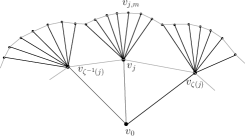
Figure 6: The first levels of the graph $\Gamma^{0}_{\Phi}$

$\bullet$ Level k:
(a) We repeat level 2 by iteration, i.e. we consider a sequence of intervals
$\{I_{j_{1}};I_{j_{1},j_{2}};\dots;I_{j_{1},j_{2},\dots,j_{k}};\dots\}$ such that:

$I_{j_{1},j_{2},\dots,j_{k}}:=I_{j_{1},j_{2},\dots,j_{k-1}}\cap\Phi^{-k+1}(I_{j_{k}})\neq\emptyset.$

Notice that if the sequence $j_{1},j_{2},\dots,j_{k}$ defines an interval of level $k$ then $j_{i+1}\neq\overline{j_{i}}$, for $1\leq i\leq k-1$, from condition (SE).
(b) A vertex $v_{j_{1},j_{2},\dots,j_{k}}$ is associated to the interval $I_{j_{1},j_{2},\dots,j_{k}}$,
(c) $v_{j_{1},j_{2},\dots,j_{k}}$ is connected to $v_{j_{1},j_{2},\dots,j_{k-1}}$ by an edge,
(d) $v_{j_{1},j_{2},\dots,j_{k}}$ is connected to $v_{j^{\prime}_{1},j^{\prime}_{2},\dots,j^{\prime}_{k}}$ if:

$I_{j^{\prime}_{1},j^{\prime}_{2},\dots,j^{\prime}_{k}}\neq I_{j_{1},j_{2},\dots,j_{k}}$ and $I_{j_{1},j_{2},\dots,j_{k}}\cap I_{j^{\prime}_{1},j^{\prime}_{2},\dots,j^{\prime}_{k}}\neq\emptyset$

.

Lemma 11.

If $\Phi$ is a piecewise homeomorphism of $S^{1}$ satisfying the condition (SE) then the graph $\Gamma^{0}_{\Phi}$, endowed with the combinatorial metric (each edge has length one), is Gromov hyperbolic with boundary $S^{1}$.

Proof.

We adapt word for word the proof in [HP]. Indeed, the essential ingredients for the proof in [HP] are the facts that each vertex is associated to a connected component of the pre-image cover with two properties:

$\bullet$ Each component has a uniformly bounded number of pre-images.
In our case, each interval has at most $2N-1$ pre-images.

$\bullet$ The size of each connected component goes to zero when the level goes to infinity.
In our case, the size of the intervals $I_{j_{1},j_{2},\dots,j_{k}}$ in the sequence of pre-images goes to zero when $k$ goes to infinity by the expansivity property (SE).

In fact a much weaker expansivity property than our condition (SE) would be enough to conclude that the graph is hyperbolic. Observe that the distance of any vertex to the base vertex is simply the level $k$ and the edge connecting $v_{j_{1},j_{2},\dots,j_{k}}$ to $v_{j^{\prime}_{1},j^{\prime}_{2},\dots,j^{\prime}_{k}}$, if any, belongs to the sphere of radius $k$ centered at the base vertex. By this observation and our definition of the edges, each sphere of radius $k$ centered at the based vertex is homeomorphic to $S^{1}$. Therefore the limit space when $k$ goes to infinity is homeomorphic to $S^{1}$ and the Gromov boundary $\partial\Gamma^{0}_{\Phi}$ is homeomorphic to $S^{1}$. ∎

4.2 The dynamical graph $\Gamma_{\Phi}$

Consider the tree $T_{\Phi}$ obtained from $\Gamma^{0}_{\Phi}$ by removing the edges on the spheres. We define on $T_{\Phi}$ an equivalence relation that identifies some vertices on some of the spheres using the specific properties (EC), (E+), (E-) of the map $\Phi$.

For $T_{\Phi}$ we use the same definitions for the intervals and vertices of Level 0, Level 1: a), b), Level 2: a), b) and Level k: a), b), c) as in $\Gamma^{0}_{\Phi}$.

Labeling the edges: The edge defined by $(v_{j_{1},j_{2},\dots,j_{k-1}},\,v_{j_{1},j_{2},\dots,j_{k}})$ is labelled by a symbol $\Psi_{j_{k}}$ and the reverse edge, the same edge but read from $v_{j_{1},j_{2},\dots,j_{k}}$, is labelled $\Psi_{\overline{j_{k}}}$.

We define a quotient map: Two vertices of $T_{\Phi}$ are identified if they belong to the same level $k>1$, we denote them $v_{j_{1},j_{2},\dots,j_{k}}$ and $v_{l_{1},l_{2},\dots,l_{k}}$, and:

• There is an integer $0\leq r<k-1$ such that:

  • $I_{j_{1},\dots,j_{i}}=I_{l_{1},\dots,l_{i}}$ as intervals in $S^{1}$, for $i=1,\dots,r$ (if $r=0$ the vertex is $v_{0}$).

  • For all $1\leq p<k-r$, the intervals $I_{j_{1},\dots,j_{r},j_{r+1},...,j_{r+p}}$ and $I_{l_{1},\dots,l_{r},l_{r+1},...l_{r+p}}$ are adjacent in the cyclique ordering of $S^{1}$ and:
    $\Phi^{r+m}(I_{j_{1},\dots,j_{r+p}})\cap\Phi^{r+m}(I_{l_{1},\dots,l_{r+p}})=\emptyset$ for all $0\leq m<p$.

• At level $k$, the intervals $I_{j_{1},\dots,j_{k}}$ and $I_{l_{1},\dots,l_{k}}$ are adjacent and:

  • $\Phi^{m}(I_{j_{1},\dots,j_{k}})\bigcap\Phi^{m}(I_{l_{1},\dots,l_{k}})=\emptyset$, for all $r<m<k$ and:
    $\Phi^{k}(I_{j_{1},\dots,j_{k}})\bigcap\Phi^{k}(I_{l_{1},\dots,l_{k}})=$ one point,

  • $\Phi^{k}(I_{j_{1},\dots,j_{k}})\bigcup\Phi^{k}(I_{l_{1},\dots,l_{k}})=$ a non degenerate interval.

Definition 2.

The dynamical graph is defined by $\Gamma_{\Phi}:=T_{\Phi}/\sim_{\Phi}$, where $\sim_{\Phi}$ is the following relation:

• Two vertices $v_{j_{1},j_{2},\dots,j_{k}}$ and $v_{l_{1},l_{2},\dots,l_{k}}$ of $T_{\Phi}$ are related if the conditions (a) and (b) above are satisfied.

• Two edges, connecting vertices from some level $m$ to level $m+1$, with the same label and starting from an identified vertex at level $m$ are identified to an edge labeled with the common label.

Lemma 12.

If $\Phi$ is a piecewise homeomorphism of $S^{1}$ satisfying the conditions (SE) and (EC), (E+), (E-) then the dynamical graph $\Gamma_{\Phi}$ is well defined.

Proof.

Let us start the study of the relation $\sim_{\Phi}$ when $r=0$ in condition (a). Condition (a2) means, in particular, that the two intervals $I_{j_{1}}$ and $I_{l_{1}}$ are adjacent, so they have a cutting point $z$ in common. Also, the $k-1$ first intervals in the sequence, up to $I_{j_{1},\dots,j_{k-1}}$ and $I_{l_{1},\dots,l_{k-1}}$ are adjacent with disjoint $\Phi^{m}$ images for $m<k-1$, by conditions (E+), (E-). The condition (b1) says that the $\Phi^{k}$ images of $I_{j_{1},\dots,j_{k}}$ and $I_{l_{1},\dots,l_{k}}$ have one point in common. This point has to be the $\Phi^{k}$ image of a cutting point $z$. By the eventual coincidence condition (EC) on $\Phi$, there is indeed an integer $k(z)$ for each cutting point, so that the two orbits of $z$ coincide after $k(z)$ iterates. Therefore condition (b1) is satisfied for this iterate $k(z)$ and such a condition is satisfied for each cutting point and therefore for each pair of adjacent intervals. Since $\Phi$ is a piecewise orientation preserving homeomorphism then condition (b2) is satisfied for the same iterate $k(z)$.

When $r>0$, for each pair of adjacent intervals $I_{j_{1},\dots,j_{r},j_{r+1}}$ and $I_{j_{1},\dots,j_{r},l_{r+1}}$ as in condition (a2), the $\Phi^{r}$ image of these intervals is as above, i.e. adjacent of level 1. Thus there is an integer $k$ for which conditions (b1) and (b2) are satisfied. The identification in Definition 2-(v) is well defined and occurs at each level after some minimal level:
$k_{0}={\rm min}\{k(j)|j=1,\dots,2N\}$, where the $k(j)$’s are the integers of condition (EC).

1) If the point $Z=\Phi^{k}(I_{j_{1},\dots,j_{k}})\bigcap\Phi^{k}(I_{l_{1},\dots,l_{k}})$ in condition (b1) is a cutting point then all edges starting from the identified vertex at level $k$ have different label and the identification (e) does not happen.

2) If, on the other hand, $Z=\Phi^{k}(I_{j_{1},\dots,j_{k}})\bigcap\Phi^{k}(I_{l_{1},\dots,l_{k}})$ belongs to the interior of an interval, say $I_{\alpha}$, then there is a sub-interval $I_{j_{1},\dots,j_{k},\alpha}$ of $I_{j_{1},\dots,j_{k}}$ and an edge labeled $\Psi_{\alpha}$ connecting $v_{j_{1},\dots,j_{k}}$ to $v_{j_{1},\dots,j_{k},\alpha}$ and similarly an edge, labeled $\Psi_{\alpha}$, connecting $v_{l_{1},\dots,l_{k}}$ to $v_{l_{1},\dots,l_{k},\alpha}$ in $T_{\Phi}$. The identification of the two vertices: $v_{j_{1},\dots,j_{k}}$ and $v_{l_{1},\dots,l_{k}}$ by $\sim_{\Phi}$ at level $k$ implies that two edges labelled $\Psi_{\alpha}$ start from the new vertex $\tilde{v}$. The identification in Definition 2(e) identifies these two edges to a single edge, connecting $\tilde{v}$ to $\tilde{v}^{1}$ at level $k+1$ with label $\Psi_{\alpha}$. This identification is well defined at level $k+1$.
The identification of type (e) is then applied inductively on each level following $k+1$. At level $k+2$, if the image $\Phi(Z)$ is a cutting point then, as in case 1), the identification of type (e) stops, i.e. the edges starting from $\tilde{v}^{1}$ have different label and no identification of type (e) occur. If $\Phi(Z)$ belongs to the interior of an interval $I_{\beta}$ then, as in case 2), two edges with label $\Psi_{\beta}$ start at $\tilde{v}^{1}$ and a new identification of type (e) occurs. The inductive identification of type (e), starting at $\tilde{v}$, depends only on the orbit $\Phi^{m}(Z)$:
- If, for some $m\geq 0$, $\Phi^{m}(Z)$ is a cutting point then the identification starting at level $k$ at $\tilde{v}$ stops at level $k+m$, as in case 1).
- If $\Phi^{m}(Z)$ is not a cutting point for all $m\geq 0$ then the identification of type (e) starting at $\tilde{v}$ does not stop and is well defined for each level $k+m$.
The dynamical graph $\Gamma_{\Phi}$ is well defined from the map $\Phi$. ∎

It is interesting to observe that the identification of type (e) is essentially a Stallings folding [Sta].

Lemma 13.

If the map $\Phi$ satisfies the ruling assumptions: (SE), (EC), (E$\pm$), (CS) then every vertex $w\neq v_{0}$ in the dynamical graph $\Gamma_{\Phi}$ of Definition 2 is identified with an interval $I_{w}$ of $S^{1}$. This interval could be of the following types:

1. $I_{w}=I_{j_{1},\dots,j_{k}}$,

2. $I_{w}=I_{j^{1}_{1},\dots,j^{1}_{k}}\bigcup I_{j^{2}_{1},\dots,j^{2}_{k}}...\bigcup I_{j^{n}_{1},\dots,j^{n}_{k}}$, for some integer $n=n(k,\Phi)$. The intervals $I_{j^{i}_{1},\dots,j^{i}_{k}}$ belong to the same level $k$ and are pairewise adjacent along $S^{1}$.

Proof.

From the proof of Lemma 12, if the vertex $w$ of $\Gamma_{\Phi}$ comes from a single vertex in $T_{\Phi}$ then it is associated to an interval of the form $I_{j_{1},\dots,j_{k}}$, this is an interval of type (i).
Otherwise $w$ comes from the identification of two vertices $v_{j_{1},j_{2},\dots,j_{k}}$ and $v_{l_{1},l_{2},\dots,l_{k}}$ satisfying conditions (a) and (b). The associated intervals in $T_{\Phi}$ are of the form: $I_{j_{1},\dots,j_{k}}$ and $I_{l_{1},\dots,l_{k}}$. They are adjacent along $S^{1}$ by condition (b), therefore $I_{w}:=I_{j_{1},\dots,j_{k}}\bigcup I_{l_{1},\dots,l_{k}}$ is an interval, associated to $w$ by the identification (v), it is called of type (ii-v). It occurs at a level $k\geq k_{0}$, where $k_{0}=min\{k(j),j=1,\dots,2N\}$.

At level $k+1$, if the case 2) in the proof of Lemma 12 is satisfied, there is an identification of type (e) of the vertices $v_{j_{1},j_{2},\dots,j_{k},\alpha}$ and $v_{l_{1},l_{2},\dots,l_{k},\alpha}$. The corresponding intervals in $T_{\Phi}$, i.e. $I_{j_{1},j_{2},\dots,j_{k},\alpha}$ and $I_{l_{1},l_{2},\dots,l_{k},\alpha}$ are adjacent along $S^{1}$ thus
$I_{w}:=I_{j_{1},j_{2},\dots,j_{k},\alpha}\bigcup I_{l_{1},l_{2},\dots,l_{k},\alpha}$ is an interval, associated to the vertex $w$ obtained by the identification of type (ii-e).

Let us observe that the neighborhood: $\widetilde{V}_{j}=V_{j}^{c_{j}}\cup V_{j}^{d_{j}}$ in the proof of Lemma 7 is exactly an interval of the form: $I_{w}:=I_{j_{1},\dots,j_{k}}\cup I_{l_{1},\dots,l_{k}}$, i.e. of type (ii-v) at level $k(j)$.

It turns out that the identifications of type (ii-v) and (ii-e), as described above, can interact. This happens in the following situations:
An identification of type (ii-e) occurs if $Z=\Phi^{k(j)}(z_{j})\in\textrm{int}(I_{\alpha})$ for some $\alpha$. Assume that $Z=\Phi^{k(j)}(z_{j})\in V_{\alpha}\cap I_{\alpha}$, where $V_{\alpha}$ is the neighborhood of the cutting point $z_{\alpha}$ described above. An identification of type (ii-e) occurs at level $k(j)+1$ and, by condition (E+), $\Phi^{m}(Z)\in I_{\delta^{m}(\alpha)}$ for $m\leq k(\alpha)-1$. This implies that $\Phi^{m}(Z)$ is not a cutting point for all $m\leq k(\alpha)-1$. By condition 2) in the proof of Lemma 12 an identification of type (ii-e) occur from level $k(j)+1$ up to level $k(j)+k(\alpha)-1$. At level $k(j)+k(\alpha)$ an identification of type (ii-e) and of type (ii-v) occur at the same level.
In this case, three intervals of the tree $T_{\Phi}$ are involved:

$I_{j_{1},...,j_{k(j)},\alpha^{\prime},...\alpha^{\prime}_{k(\alpha)}}$, $I_{j_{1},...,j_{k(j)},\alpha,...\alpha_{k(\alpha)}}$, $I_{l_{1},...,l_{k(j)},\alpha,...\alpha_{k(\alpha)}}$, where $\alpha^{\prime}=\zeta^{-1}(\alpha)$.

As in the previous cases, these intervals are pairewise adjacent along $S^{1}$ and the identification of both types (ii-e) and (ii-v) is associated to the union:
$I_{w}:=I_{j_{1},...,j_{k(j)},\alpha^{\prime},...\alpha^{\prime}_{k(\alpha)}}\bigcup I_{j_{1},...,j_{k(j)},\alpha,...\alpha_{k(\alpha)}}\bigcup I_{l_{1},...,l_{k(j)},\alpha,...\alpha_{k(\alpha)}}$, this is an interval.

For the next levels, the two cases 1) or 2) in the proof of Lemma 12 might occur, depending on the orbits of each cutting points, i.e. $z_{j}$ and $z_{\alpha}$.

The phenomenon described above, where two identifications of type (ii-e) and (ii-v) arise for the same vertex, can possibly occur at any level large enough. The intervals in $T_{\Phi}$ that are involved are pairewise adjacent, as above, and the union of these interval is an interval. The number $n_{m}$ of these intervals depends on the map $\Phi$ via the orbits of the cutting points and on the level $m$.

From the proof of Lemma 12 there is a difference between the vertices of type (ii) obtained after an identification of type (v) or type (e) in Definition 2. A vertex obtained by an identification of type (v) has two incoming edges, i.e. from level $k-1$ to level $k$. A vertex obtained by an identification of type (e) has only one incoming edge, as the vertices of type (i). If necessary, we will mark the difference by denoting the corresponding vertices or intervals of type (ii-v) or type (ii-e). ∎

Proposition 3.

If $\Phi$ and $\Phi^{\prime}$ are two piecewise homeomorphisms of $S^{1}$ with the same combinatorics, i.e. the same permutations $\zeta$ and $\iota$, the same properties (SE), (EC), (E+), (E-), (CS) with the same slope, then the graphs $\Gamma_{\Phi}$ and $\Gamma_{\Phi^{\prime}}$ are homeomorphic.

Proof.

Since the combinatorics are the same, all the combinatorial data used in the constructions: $k(j)$, $\gamma$ and $\delta$ are the same for $\Phi$ and $\Phi^{\prime}$. The identification of type (ii-v) defines vertices with two incoming edges, and $2N-2$ outgoing edges, by condition (7) in the proof of Lemma 7. The vertices of types (i) and (ii-e) have one incoming edge and $2N-1$ out going edges by condition (SE). The identifications process could be quite different for different maps but each resulting vertex has the same structure, even as a labeled graph. Therefore the two graphs are homeomorphic. ∎

Lemma 14.

Let $\Phi:S^{1}\rightarrow S^{1}$ satisfying the conditions (SE), (EC), (E+), (E-), (CS) then there exists $\Phi^{\prime}:S^{1}\rightarrow S^{1}$ with the same combinatorics as $\Phi$ so that the identifications of type (ii) in Lemma 13 are all 2 to 1.

Proof.

The idea is to change the map $\Phi$ by changing the cutting points while preserving the combinatorics. We replace $\Phi$ by the affine map $\widetilde{\Phi}$ via the conjugacy of condition (CS), the combinatorics are evidently the same. Consider the neighborhood $\widetilde{V}_{j}$ of Lemma 7 and the $\lambda$-affine extension $\widetilde{\Phi}_{j}^{\tilde{V}}$ of Lemma 8. Lemma 8 (a) implies:
$\widetilde{\Phi}_{j}^{\tilde{V}}(V_{j})\subset\tilde{I}_{\delta(j)}\setminus\widetilde{V}_{\delta(j)}$ and conditions (E$\pm$), together with the definition of $V_{j}$ give:

$$\widetilde{\Phi}^{m}(\widetilde{\Phi}_{j}^{\tilde{V}}(\widetilde{V}_{j}))\in\tilde{I}_{\delta^{m+1}(j)}\textrm{ and }\widetilde{\Phi}^{m}(\widetilde{\Phi}_{\zeta^{-1}}^{\tilde{V}}(\widetilde{V}_{j}))\in\tilde{I}_{\gamma^{m+1}(\zeta^{-1})},\textrm{ for }0\leq m\leq k(j)-2.$$ (29)

The condition (EC) gives $Z=\widetilde{\Phi}^{k(j)}(\tilde{z}_{j})\in\tilde{I}_{\alpha}$, for some $\alpha\in\{1,\dots,2N\}$. Consider the fixed point $p^{\alpha}\in\tilde{I}_{\alpha}$ of $\widetilde{\Phi}_{\alpha}$, given by condition (SE). The definition of the involution $\iota$ and condition (SE) implies that the fixed point $p^{\alpha}$ belongs to the subinterval $I_{\alpha,\alpha}$ which is disjoint from $I_{\alpha,\delta(\alpha)}\cup I_{\alpha,\gamma(\alpha)}$. By definition of the intervals $V_{j}$ in Lemma 7 we obtain: $p^{\alpha}\notin V_{\alpha}\cup V_{\zeta(\alpha)}$.

If $Z=p^{\alpha}$ then we do not change the cutting point $z_{j}$.

If $Z\neq p^{\alpha}$ then either $p^{\alpha}\in\widetilde{\Phi}^{k(j)}(V_{j}^{+})$ for $V_{j}^{+}:=\widetilde{V}_{j}\cap\widetilde{I}_{j}$ or $p^{\alpha}\in\widetilde{\Phi}^{k(j)}(V_{j}^{-})$ for $V_{j}^{-}:=\widetilde{V}_{j}\cap\widetilde{I}_{\zeta^{-1}(j)}$. Assume, for instance, that $p^{\alpha}\in\widetilde{\Phi}^{k(j)}(V_{j}^{+})$ and let $p^{\alpha}_{j}=\widetilde{\Phi}^{-k(j)}(p^{\alpha})\in V_{j}^{+}\subset\tilde{I}_{j}$, the other case is symmetric. The goal is to transform the map $\widetilde{\Phi}$ to $\Phi^{\prime}$ so that $p^{\alpha}_{j}$ is the new cutting point. Since $p^{\alpha}_{j}\in V_{j}^{+}\subset\tilde{I}_{j}$ we define $\Phi^{\prime}_{j}=\widetilde{\Phi}_{j}$ on the interval $[p^{\alpha}_{j},\tilde{z}_{\zeta(j)})$. We define the map $\Phi^{\prime}_{\zeta^{-1}(j)}$ by the $\lambda$-affine extension of $\widetilde{\Phi}_{\zeta^{-1}(j)}$, i.e. from the interval $[\tilde{z}_{\zeta^{-1}(j)},\tilde{z}_{j})$ to $[\tilde{z}_{\zeta^{-1}(j)},p^{\alpha}_{j})$ as in (9). We apply the same construction for each cutting point. The permutations $\zeta$ and $\iota$ as well as all the $k(j)$ are the same for $\Phi^{\prime}$ as for $\Phi$. The properties in (29), coming from Lemma 8(a) and (E$\pm$) for $\Phi$, imply that the conditions (E$\pm$) are satisfied by $\Phi^{\prime}$. The condition (EC) is satisfied by $\Phi^{\prime}$ from the equality (b) in Lemma 8. Condition (CS), with slope $\lambda$ is satisfied by $\Phi^{\prime}$ by construction. The two maps $\Phi$ and $\Phi^{\prime}$ have thus the same combinatorics.

The choice of the new cutting point $p^{\alpha}_{j}$ of $\Phi^{\prime}$ implies that $Z^{\prime}=\Phi^{\prime k(j)}(p^{\alpha}_{j})=p^{\alpha}$ which is fixed by $\Phi^{\prime}$ since $\Phi^{\prime}=\widetilde{\Phi}$ outside the set $\bigcup V_{j}$ and we observed that $p^{\alpha}\notin V_{\alpha}\cup V_{\zeta(\alpha)}$. Therefore we obtain: $\Phi^{\prime m}(Z^{\prime})=p^{\alpha}$ for all $m\geq 0$ and thus this orbit is always outside the set $\bigcup V_{j}$. By the proof of Lemma 13, the identifications of type (ii-e) occur at all levels after level $k(j)$ and do not interact with identifications of type (ii-v). Therefore the identifications of type (ii) in Lemma 13 are all with two intervals, i.e. are 2 to 1. ∎

Remark 2.

All the cutting points of the new map $\Phi^{\prime}$ are pre-periodic and thus the map satisfies a Markov property.

Lemma 15.

The two graphs $\Gamma_{\Phi^{\prime}}$ and $\Gamma^{0}_{\Phi^{\prime}}$, endowed with the combinatorial metric (every edge has length one), are quasi-isometric.

Proof.

Let us denote by $d_{\Gamma_{\Phi^{\prime}}^{0}}$ and $d_{\Gamma_{\Phi^{\prime}}}$ the combinatorial distances in $\Gamma_{\Phi^{\prime}}^{0}$ and $\Gamma_{\Phi^{\prime}}$. The two sets of vertices $V(\Gamma_{\Phi^{\prime}}^{0})$ and $V(\Gamma_{\Phi^{\prime}})$ are related by a map:
${\cal V}:V(\Gamma_{\Phi^{\prime}}^{0})\rightarrow V(\Gamma_{\Phi^{\prime}})$ which is induced by the relation $\sim_{\Phi}$ of Definition 2 and is at most 2 to 1 by Lemma 14. Each vertex $v\in V(\Gamma_{\Phi^{\prime}}^{0})\setminus\{v_{0}\}$ is identified with an interval $I_{v}:=I_{j_{1},\dots,j_{k}}$ and thus with a vertex of the tree $T_{\Phi^{\prime}}$. Two vertices of $\Gamma_{\Phi^{\prime}}^{0}$ with the same $\cal{V}$-image correspond to adjacent intervals at the same level $k$, they are at distance one in $\Gamma_{\Phi^{\prime}}^{0}$.

Two vertices connected by an edge on a sphere $S_{p}^{0}$ of radius $p$ centered at the base vertex $v_{0}$ in $\Gamma_{\Phi^{\prime}}^{0}$ are mapped either to a single vertex in the sphere $S_{p}$ of radius $p$, centered at $v_{0}$ in $\Gamma_{\Phi^{\prime}}$ or to two distinct vertices on the same sphere. These two vertices are connected in $\Gamma_{\Phi^{\prime}}$ by a path of length at most $k(j)$, for some $j\in\{1,\dots,2N\}$, where $k(j)$ is the integer in the condition (EC). We define $K_{\Phi^{\prime}}:={\rm max}\{k(j)|j=1,\dots,2N\}$ then we obtain:

$d_{\Gamma_{\Phi^{\prime}}}({\cal V}(v^{0}_{\alpha}),{\cal V}(v^{0}_{\beta}))\leq K_{\Phi^{\prime}}.d_{\Gamma_{\Phi^{\prime}}^{0}}(v^{0}_{\alpha},v^{0}_{\beta})+C$,

for any pair of vertices $(v^{0}_{\alpha},v^{0}_{\beta})$ in $V(\Gamma_{\Phi^{\prime}}^{0})\times V(\Gamma_{\Phi^{\prime}}^{0})$.
Indeed a minimal length path between $v^{0}_{\alpha}$ and $v^{0}_{\beta}$ is a concatenation of some paths along the spheres centered at $v_{0}$ and some paths along rays starting at $v_{0}$. The length of the paths along the rays are preserved by the map ${\cal V}$ and the length of the paths along the spheres are at most expanded by a factor bounded by $K_{\Phi^{\prime}}$. On the other direction, the same observation and the fact that ${\cal V}$ could identify at most two vertices implies:

$d_{\Gamma_{\Phi^{\prime}}}({\cal V}(v^{0}_{\alpha}),{\cal V}(v^{0}_{\beta}))\geq\frac{1}{K_{\Phi^{\prime}}}d_{\Gamma_{\Phi^{\prime}}^{0}}(v^{0}_{\alpha},v^{0}_{\beta})-C$.

∎

Corollary 1.

The graph $\Gamma_{\Phi}$, with the combinatorial distance, is hyperbolic with boundary homeomorphic to $S^{1}$.

Proof.

A metric space quasi-isometric to a Gromov hyperbolic space is Gromov hyperbolic with the same boundary [GdlH]. By Lemmas 11 and 15 the graph $\Gamma_{\Phi^{\prime}}$ is hyperbolic with boundary $S^{1}$. By Proposition 3 the same property is satisfied by $\Gamma_{\Phi}$. ∎

5 An action of $G_{X_{\Phi}}$ on $\Gamma_{\Phi}$

The groups $G_{X_{\Phi}}$ of Definition 1 are the main object of study for the rest of the paper, they are subgroups of $\textrm{Homeo}^{+}(S^{1})$. From Theorem 1, some relations are satisfied among the generators defined in §3, the cutting point relations, but we don’t know if this is the whole set of relations. The main goal is to understand these groups. The classical method to study such groups is via a geometric action on a metric space. The graph $\Gamma_{\Phi}$ of the previous section has been defined for that purpose, it is a hyperbolic metric space that reflects the dynamics of the map $\Phi$. It is a candidate metric space but an action of $G_{X_{\Phi}}$ on $\Gamma_{\Phi}$ has to be defined, via the data we have i.e. the dynamics of the map $\Phi$.

Recall that a geometric action of a group on a metric space is a morphism, acting by isometries that is co-compact and properly discontinuous.
By Lemma 13, each vertex $v\in V(\Gamma_{\Phi})$ is identified with an interval $I_{v}\subset S^{1}$ and each $g\in G_{X_{\Phi}}$ is, in particular, a homeomorphism of $S^{1}$. We need to understand, for each $g\in G_{X_{\Phi}}$ how the interval $g(I_{v})$ is related to some $I_{w}$ for $w\in V(\Gamma_{\Phi})$.
An ideal situation would be that for “all $v$ and all $g$ there is $w$ so that $g(I_{v})=I_{w}$”, we will see immediately that this ideal situation does not happens for all vertices (see Lemma 16). The idea for defining an action is to weaken this ideal situation and to find an interval $I_{w}$ so that $g(I_{v})$ and $I_{w}$ are “close enough”, i.e. to admit a controlled error.

5.1 A preliminary step

Let us describe how the generators $\varphi_{j}\in X_{\Phi}$ of the group do act on the partition intervals $I_{m}$ for all $m\in\{1,\dots,2N\}$, i.e. on the intervals associated to vertices of level 1 in $\Gamma_{\Phi}$. Recall that in this section we do not distinguish between the intervals $I_{j}$ and $\tilde{I_{j}}$.

Lemma 16.

If $\Phi$ is a piecewise homeomorphism of $S^{1}$ satisfying the conditions (SE), (E-), (E+), (EC) and (CS), let $\varphi_{j}\in X_{\Phi}$ be a generator of the group $G_{X_{\Phi}}$ given by Theorem 1. If $I_{m}$ is a partition interval, $m\in\{1,\dots,2N\}$ then $\varphi_{j}(I_{m})$ satisfies one of the following conditions:

1. If $m=j$ then: $\varphi_{j}(I_{j})\cap I_{k}\neq\emptyset$ for all $k\neq\iota(j)$.

2. For all $m\neq j,\zeta^{\pm 1}(j)$ then: $\varphi_{j}(I_{m})=I_{\iota(j),m}$.

3. $\varphi_{j}(I_{\zeta(j)})=I_{\iota(j),\zeta(j)}\cup L_{\iota(j)}$ and $\varphi_{j}(I_{\zeta^{-1}(j)})=I_{\iota(j),\zeta^{-1}(j)}\cup R_{\iota(j)}$,
   where $L_{\iota(j)}$ and $R_{\iota(j)}$ are defined in (3), they satisfy:
   $L_{\iota(j)}\subsetneq I_{\gamma(j)),\gamma^{2}(j),\dots,\gamma^{k(\zeta(j))-1}(j)}$, and $R_{\iota(j)}\subsetneq I_{\delta(j),\delta^{2}(j),\dots,\delta^{k(j)-1}(j)}$,

   where $k(\zeta(j))$ and $k(j)$ are the integers of condition (EC).

Proof.

The proof is a case by case study.

(a) This is simply condition (SE) on the map $\Phi$.

(b) By Lemma 6 and the choices made in Theorem 1, the generators satisfy:
$(\varphi_{j})_{|\widetilde{\Phi}_{\iota(j)}(I_{\iota(j)})}=(\widetilde{\Phi}_{\iota(j)})^{-1}_{|\widetilde{\Phi}_{\iota(j)}(I_{\iota(j)})}$. Condition (SE) implies that: $\widetilde{\Phi}_{\iota(j)}(I_{\iota(j)})\cap I_{m}=I_{m}$, for all $m\neq j,\zeta^{\pm 1}(j)$. Therefore we obtain: $I_{\iota(j)}\cap\widetilde{\Phi}^{-1}_{|I_{\iota(j)}}(I_{m})=\widetilde{\Phi}^{-1}_{|I_{\iota(j)}}(I_{m})$ which reads: $I_{\iota(j),m}=\varphi_{j}(I_{m})$ (see Figure 7).

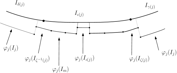
Figure 7: Image of the intervals $I_{m}$ under $\varphi_{j}$

(c) The two situations are symmetric, we restrict to one of them, for instance to $\varphi_{j}(I_{\zeta(j)})$. By condition (SE), applied to $I_{j}$ and $I_{\iota(j)}$, we have:

(i) $\varphi_{j}(I_{j})\cap I_{\gamma(j)}\subsetneq I_{\gamma(j)}$, and (ii) $\varphi_{\iota(j)}(I_{\iota(j)})\cap I_{\zeta(j)}\subsetneq I_{\zeta(j)}$.

By (i) and the continuity of $\varphi_{j}$ we have $L_{\iota(j)}=\varphi_{j}(I_{\zeta(j)})\cap I_{\gamma(j)}\neq\emptyset,$ and by (ii) we have $\varphi_{j}(I_{\zeta(j)})\cap I_{\iota(j)}\neq\emptyset$. On the other hand, by definition of the generators $\varphi_{j}$ and Lemma 6 we have:

$\varphi_{j}(I_{\zeta(j)})\cap I_{\iota(j)}=\widetilde{\Phi}^{-1}_{|I_{\iota(j)}}(I_{\zeta(j)})\cap I_{\iota(j)}=I_{\iota(j),\zeta(j)}.$

Thus, we obtain $\varphi_{j}(I_{\zeta(j)})=I_{\iota(j),\zeta(j)}\cup L_{\iota(j)}$ (see Figure 7).

To complete the proof we verify the properties of the interval $L_{\iota(j)}$ (resp. $R_{\iota(j)}$). With the notations of the cutting points, this interval is:

$L_{\iota(j)}=[\varphi_{j}(z_{\zeta(j)}),z_{\iota(j)}]$ (see Figure 7).

By condition (E+) at $z_{\zeta(j)}$ we have: $\forall i,0\leq i\leq k(\zeta(j))-2:\tilde{\Phi}^{i}(\tilde{\Phi}_{j}(z_{\zeta(j)}))\in I_{\gamma^{i+1}(j)}$. For $i=0$: $\tilde{\Phi}_{j}(z_{\zeta(j)})=\varphi_{j}(z_{\zeta(j)})\in I_{\gamma(j)}$, and for $i=1$: $\tilde{\Phi}(\tilde{\Phi}_{j}(z_{\zeta(j)}))\in I_{\gamma^{2}(j)}$, this last condition means that the $\tilde{\Phi}$ image of the point $\varphi_{j}(z_{\zeta(j)})\in I_{\gamma(j)}$ belongs to the same partition interval as the $\tilde{\Phi}$ image of the cutting point $z_{\iota(j)}$. Therefore the point $\varphi_{j}(z_{\zeta(j)})$ belongs to the interior of the last sub-interval of level 2 of the partition interval $I_{\gamma(j)}$ which is $I_{\gamma(j),\gamma^{2}(j)}$. This implies that: $L_{\iota(j)}\subsetneq I_{\gamma(j),\gamma^{2}(j)}$ which is part of the statement. At this stage we only use the first iterate ($i=1$) in conditions (E+). The proof of (c) is completed by applying the same arguments for all iterates: $i\leq k(\zeta(j))-2$ in condition (E+), we obtain:

$L_{\iota(j)}\subsetneq I_{\gamma(j),\gamma^{2}(j),\dots,\gamma^{k(\zeta(j))-1}(j)}.$

This completes the proof of statement (c) in this case. The symmetric situation in case (c), is obtained by replacing $\zeta$ by $\zeta^{-1}$, $\gamma$ by $\delta$ and condition (E+) by (E-). ∎

5.2 Additional properties of $\Gamma_{\Phi}$

From the proof of Lemma 16, the intervals of level $m\leq k(j)-2$ in the tree $T_{\Phi}$ that are extrem in the interval $I_{j}$, i.e. contain a cutting point, are of the form:

$$I_{j,\delta(j),\dots,\delta^{m}(j)}\textrm{ and }I_{j,\gamma(j),\dots,\gamma^{m}(j)}.$$ (30)

The intervals of type (ii) and level $k(j)$ in the proof of Lemma 13 are thus of the form:

$$I_{\tilde{v}_{j}}:=I_{j,\delta(j),\dots,\delta^{k(j)-1}(j)}\cup I_{\zeta^{-1}(j),\gamma(\zeta^{-1}(j)),\dots,\gamma^{k(j)-1}(\zeta^{-1}(j))},$$ (31)

where the first interval is extrem of level $k(j)$ on the (+) side of $\tilde{z}_{j}$ and the second is extrem on the (-) side of the same cutting point. This interval is of type (ii-v). It contains sub-intervals of level $k(j)+1$ and possibly one with the cutting point $z_{{}_{j}}$ in its interior, as in case 2) in the proof of Lemma 12:

$I_{\tilde{v}_{j},\alpha}:=I_{\zeta^{-1}(j),\gamma(\zeta^{-1}(j)),\dots,\gamma^{k(j)-1}(\zeta^{-1}(j)),\alpha}\cup I_{j,\delta(j),\dots,\delta^{k(j)-1}(j),\alpha}$,

where $\alpha$ satisfies (7), this interval is of type (ii-e).

More generaly, from Definition 2 of the equivalence relation $\sim_{\Phi}$, an interval of type (ii-v) is of the form:

$$I_{\tilde{v}_{\ell,j}}:=I_{\ell,\zeta^{-1}(j),\gamma(\zeta^{-1}(j)),\dots,\gamma^{k(j)-1}(\zeta^{-1}(j))}\cup I_{\ell,j,\delta(j),\dots,\delta^{k(j)-1}(j)},$$ (32)

where $\ell$ is a finite sequence (possibly empty) in $\{1,\dots,2N\}$. The corresponding vertices are denoted: $\tilde{v}_{j}$, $\tilde{v}_{j,\alpha}$ and $\tilde{v}_{\ell,j}$.
The next result induces an additional structure of the graph $\Gamma_{\Phi}$ around each vertex.

Proposition 4.

If the map $\Phi$ satisfies the ruling conditions: (SE), (EC), (E+), (E-) then the set of edges that are incident to a vertex $v\in V(\Gamma_{\Phi})$ admit a natural cyclic ordering induced by the cyclic ordering of the partition intervals $I_{j}$ along $S^{1}$. In addition each vertex has valency $2N$.

Proof.

By definition of $\Gamma_{\Phi}$, the cyclic ordering of the intervals $I_{j}$ along $S^{1}$ defines a cyclic ordering of the vertices of level $1$ and thus a cyclic ordering on the edges incident at $v_{0}$. By Proposition 3 the structure of $\Gamma_{\Phi}$ depends only on the combinatorics of the map $\Phi$. To simplify the arguments we assume that the identification of type (ii) are all 2 to 1, as in Lemma 14.

If $v=v_{j_{1},\dots,j_{t}}\in V(\Gamma_{\Phi})$ is a vertex of type (i) or (ii-e) and level $t\geq 1$:
Then it is connected to one vertex of level $t-1$, i.e. to $v=v_{j_{1},\dots,j_{t-1}}$, and to $2N-1$ vertices of level $t+1$, by condition (SE). At level $t+1$, these vertices $w_{i}$ are ordered by the ordering of the sub-intervals $I_{w_{i}}$ along the interval $I_{v}$ as sub-intervals of $S^{1}$. Recall that the ordering along $S^{1}$ is expressed by the permutation $\zeta$ (see $\S$ 2.1). By condition (SE) these vertices at level $t+1$ are:

$v_{j_{1},\dots,j_{t},{\zeta(\overline{j_{t}})}},\,v_{j_{1},\dots,j_{t},\zeta^{2}(\overline{j_{t}})},\dots,v_{j_{1},\dots,j_{t},\zeta^{2N-1}(\overline{j_{t}})}$.

The edges arriving at these vertices, from $v$, are labelled respectively:

$\Psi_{\zeta(\overline{j_{t}})},\dots,\Psi_{\zeta^{2N-1}(\overline{j_{t}})}$.

The vertex at level $t-1$ is $v_{j_{1},\dots,j_{t-1}}$ and the reverse edge, i.e from $v$ to it, is labelled $\Psi_{\overline{j_{t}}}$. Therefore, the vertices of type (i) or (ii-e) admit a cyclic ordering of the edges induced by the permutation $\zeta$.

If $v$ is a vertex of type (ii-v):
Then, there is $j\in\{1,\dots,2N\}$ and a finite sequence $\ell$ in $\{1,\dots,2N\}$ so that $v$ is identified with an interval $I_{\tilde{v}_{\ell,j}}$ as in (32).

From the equivalence relation $\sim_{\Phi}$, the vertex $v$ has two incoming edges and they are adjacent by Lemma 4. These two edges are labelled, reading from $v$, as:

$\Psi_{\overline{\delta^{k(j)-1}(j)}}\textrm{ and }\Psi_{\overline{\gamma^{k(j)-1}(\zeta^{-1}(j))}}$.

And there are $2N-2$ out-going edges, ordered by the ordering along $S^{1}$. By condition (7) in the proof of Lemma 7, they are labelled as:

$\Psi_{\zeta(\overline{\gamma^{k(j)-1}(\zeta^{-1}(j))})},\dots,\Psi_{\zeta^{2N-2}(\overline{\gamma^{k(j)-1}(\zeta^{-1}(j))})}$.

In all cases, i.e. for the vertices of type (i), (ii-e) or (ii-v), $2N$ edges are incident at $v$ and they are cyclically ordered by the permutation $\zeta$ and thus by the ordering of the intervals along $S^{1}$. ∎

Corollary 2.

Each pair of consecutive edges for the natural cyclic ordering, at any vertex $v$, is associated to exactly one “cutting point” relation of Theorem 1.

Proof.

By the proof of Theorem 1, each “cutting point” relation is associated to a cycle of the permutation $\delta$ or $\gamma$. From the proof of Lemma 16, a cycle of the permutation $\delta$ or $\gamma$ is also associated to the iteration of $\Phi$ via conditions (E+), (E-). In term of the edges in $\Gamma_{\Phi}$, the cycle defines the following loop, given by the sequence of labeled edges:

$\Psi_{\zeta^{-1}(j)},\;\Psi_{\gamma(\zeta^{-1}(j))},\dots,\;\Psi_{\gamma^{k(j)-1}(\zeta^{-1}(j))},\;\Psi_{\overline{\delta^{k(j)-1}(j)}},\dots,\;\Psi_{\overline{\delta(j)}},\;\Psi_{\overline{j}},$

for each $j=1,\dots,2N$. The two edges labeled $\Psi_{\zeta^{-1}(j)}$ and $\Psi_{j}$ are adjacent by definition of $\zeta$. Moreover, since the cycles of the permutations are disjoint, each pair of consecutive edges is associated to exactly one “cutting point” relation. ∎

Remark 3.

Any vertex $v\in V(\Gamma_{\Phi})$ is contained in a compact set ${\cal{C}}_{v}$ defined by the union of the loops associated to the pairs of adjacent edges in Corollary 2 (see Figure 8 for ${\cal{C}}_{v_{0}}$). The extreme points of the compact set ${\cal{C}}_{v_{0}}$ correspond to vertices of type (ii-v), the other vertices are of type (i) according to Lemma 13.

Figure 8: The compact set ${\cal{C}}_{v_{0}}$ in $\Gamma_{\Phi}$

5.3 How the generators do act on the vertices of ${\cal{C}}_{v_{0}}$?

In this part we study the action of each generator $\varphi_{j}$ on the set of intervals corresponding to the vertices of the compact set ${\cal{C}}_{v_{0}}$. Lemma 16 is the first step and most of the arguments are exactly like in its proof. Observe that ${\cal{C}}_{v_{0}}$ is contained in the ball of $\Gamma_{\Phi}$: $\textrm{Ball}(v_{0},K_{\Phi})$ where the radius $K_{\Phi}=\textrm{max}\{k(j):j\in\{1,\dots,2N\}\}$ was defined in the proof of Lemma 15.

Proposition 5.

With the above definitions and notations, the image under $\varphi_{j}$ of the intervals $I_{v}$ of type (i), associated to the vertices in ${\cal{C}}_{v_{0}}$ by Lemma 13, are given by the following cases:

1. If the cutting point $z_{j}$ is a boundary point of $I_{v}$ then, for $0\leq m\leq k(j)-2$:

   1. if $I_{v}=I_{j,\delta(j),\delta^{2}(j),\dots,\delta^{m}(j)}$ then $\varphi_{j}(I_{v})\subset I_{\delta(j),\dots,\delta^{m}(j)}$ with $\varphi_{j}(I_{v})\cap I_{\delta(j),\dots,\delta^{m}(j),\alpha}\neq\emptyset$, for all possible such $\alpha\in\{1,\dots,2N\}$, i.e. all except one,

   2. if $I_{v}=I_{\zeta^{-1}(j),\dots,\gamma^{m}(\zeta^{-1}(j))}$ then $\varphi_{j}(I_{v})=I_{\iota(j),\zeta^{-1}(j),\dots,\gamma^{m}(\zeta^{-1}(j))}\cup R_{\iota(j)}$, where $R_{\iota(j)}$ satisfies the properties (c) in Lemma 16.

2. If $z_{\zeta(j)}$ is a boundary point of $I_{v}$ then, for $0\leq m\leq k(\zeta(j))-2$:

   1. if $I_{v}=I_{j,\gamma(j),\delta^{2}(j),\dots,\gamma^{m}(j)}$ then $\varphi_{j}(I_{v})\subset I_{\gamma(j),\dots,\gamma^{m}(j)}$ with $\varphi_{j}(I_{v})\cap I_{\gamma(j),\dots,\gamma^{m}(j),\alpha}\neq\emptyset$, for all possible such $\alpha\in\{1,\dots,2N\}$, i.e. all except one,

   2. if $I_{v}=I_{\zeta(j),\delta(\zeta(j))\dots,\delta^{m}(\zeta(j))}$ then $\varphi_{j}(I_{v})=I_{\iota(j),\zeta(j),\dots,\delta^{m}\zeta(j)}\cup L_{\iota(j)}$, where $L_{\iota(j)}$ satisfies the properties (c) in Lemma 16.

3. If $I_{v}$ is of type (i) and does not contain $z_{j}$ or $z_{{}_{\zeta(j)}}$ as a boundary point then it has the form: $I_{v}=I_{j_{1},\dots,j_{r}}$ for $j_{1}\neq j$ and $\varphi_{j}(I_{v})=I_{\iota(j),j_{1},\dots,j_{r}}$.

Proof.

Let $v\in V(\Gamma_{\Phi})\cap{\cal{C}}_{v_{0}}$.

1) If the cutting point $z_{j}$ belongs to the boundary of $I_{v}$ and $v$ is a vertex of type (i) according to Lemma 13 then it is given by (30). Let us consider this set of intervals.

(a) If $I_{v}=I_{j,\delta(j),\delta^{2}(j),\dots,\delta^{m}(j)}$.
For $m=1$, the argument in the proof of Lemma 16-(a) implies: $\varphi_{j}(I_{j,\delta(j)})\subset I_{\delta(j)}$ and $\varphi_{j}(I_{j,\delta(j)})\cap I_{\delta(j),\alpha}\neq\emptyset$ for all such possible $\alpha$.
The same argument applies for all $1\leq m\leq k(j)-2$ and we obtain the statement (1-a) in this case.

(b) If $I_{v}=I_{\zeta^{-1}(j),\gamma(\zeta^{-1}(j)),\dots,\gamma^{m}(\zeta^{-1}(j))}$, the arguments in the proof of Lemma 16-(c) apply and we obtain, for all $1\leq m\leq k(j)-2$:

$\varphi_{j}(I_{\zeta^{-1}(j),\gamma(\zeta^{-1}(j)),\gamma^{2}(\zeta^{-1}(j)),\dots,\gamma^{m}(\zeta^{-1}(j))})=I_{\iota(j),\zeta^{-1}(j),\gamma(\zeta^{-1}(j)),\dots,\gamma^{m}(\zeta^{-1}(j))}\cup R_{\iota(j)}$,
where $R_{\iota(j)}\subsetneq I_{\delta(j),\delta^{2}(j),\dots,\delta^{k(j)-1}(j)}$ by Lemma 16-(c).

2) If $z_{j}$ is replaced by $z_{{}_{\zeta(j)}}$ then $\delta(j)$ is replaced by $\gamma(j)$, the condition (E+) is replaced by (E-) and the same arguments apply, by symmetry.

3) If the interval $I_{v}$ of type (i), level $r>1$ and does not contain the cutting points $z_{\zeta(j)}$ or $z_{j}$ then it has the form $I_{j_{1},...,j_{r}}$ with $j_{1}\neq j$ and if $j_{1}=\zeta^{\pm 1}(j)$ then $j_{2}\neq\gamma(j)\textrm{ or }\delta(\zeta^{-1}(j))$. In these cases, the arguments in Lemma 16-(b) apply and $\varphi_{j}(I_{j_{1},...,j_{r}})=I_{\iota(j),j_{1},...,j_{r}}$. ∎

For the next result we consider the intervals of type (ii) of Lemma 13. They are associated to the “extreme points” of the compact ${\cal{C}}_{v_{0}}$ (see Figure 8). At level $k(j)$, around $z_{j}$, they are given by the intervals $I_{\tilde{v}_{j}}$ in (31).

Proposition 6.

With the above definitions and notations the image, under $\varphi_{j}$, of the intervals $I_{\tilde{v}_{m}}$ of type (ii) associated to the vertices in ${\cal{C}}_{v_{0}}$ are given by the following cases:

1. $\varphi_{j}(I_{\tilde{v}_{{}_{j}}})\subset I_{\delta(j),\delta^{2}(j),\dots,\delta^{k(j)-1}(j)}$ (resp. $\varphi_{j}(I_{\tilde{v}_{{}_{\zeta(j)}}})\subset I_{\gamma(j),\gamma^{2}(j),\dots,\gamma^{k(\zeta(j))-1}(j)}$) and it intersects all sub intervals of level $k(j)$ (resp. $k(\zeta(j))$ ), except one.

2. $\varphi_{j}(I_{\tilde{v}_{{}_{l}}})=I_{\iota(j),\tilde{v}_{l}},$ with the notation (32) for $l\notin\{j,\zeta(j)\}.$

Proof.

1) From the definition of the neighborhood $V_{j}$ in Lemma 7, we observe that the interval $I_{\tilde{v}_{j}}$ of (31) satisfies : $V_{j}=I_{\tilde{v}_{j}}$.

The generators $\varphi_{j}$ given by Theorem 1, together with Lemma 8 gives:

$\varphi_{j}(I_{\tilde{v}_{j}})\subset I_{\delta(j)}\setminus I_{\tilde{v}_{\delta(j)}}$.

From the construction of the neighborhood $V_{j}$ in Lemma 7 we obtain:
$\Phi^{m}(\varphi_{j}(I_{\tilde{v}_{j}}))\subset I_{{\delta}^{m+1}(j)}$ for all $m=0,\dots,k(j)-2$, and thus : $\varphi_{j}(I_{\tilde{v}_{j}})\subset I_{\delta(j),\delta^{2}(j),\dots,\delta^{k(j)-1}(j)}$.

For the next iterate of $\Phi$, the condition (7) implies:

$\Phi^{k(j)-1}(\varphi_{j}(I_{\tilde{v}_{j}}))\cap I_{m}\neq\emptyset$ for all $m\neq\overline{\gamma^{k(j)-1}}(\zeta^{-1}(j)),\overline{\delta^{k(j)-1}}(j)$.

We observe that $I_{\tilde{v}_{\delta(j)}}\cap I_{\delta(j)}$ is a subinterval of $I_{\delta(j),\delta^{2}(j),\dots,\delta^{k(j)}(j)}$ of level $k(j)$ and by Lemma 8-(a) we have: $\varphi_{j}(I_{\tilde{v}_{j}})\cap I_{\tilde{v}_{\delta(j)}}=\emptyset$. Therefore $\varphi_{j}(I_{\tilde{v}_{j}})$ intersects all subintervals of level $k(j)$ of $I_{\delta(j),\delta^{2}(j),\dots,\delta^{k(j)-1}(j)}$, except one, i.e. $I_{\tilde{v}_{\delta(j)}}\cap I_{\delta(j)}$.

If $I_{\tilde{v}_{j}}$ is replaced by $I_{\tilde{v}_{{}_{\zeta(j)}}}$ then the same arguments apply by replacing $\delta(j)$ with $\gamma(j)$.

2) For $I_{\tilde{v}_{l}}=I_{\zeta^{-1}(l),\gamma(\zeta^{-1}(l)),\dots,\gamma^{k(l)-1}(\zeta^{-1}(l))}\cup I_{l,\delta(l),\dots,\delta^{k(l)-1}(l)},$ we have

$\varphi_{j}(I_{\zeta^{-1}(l),\gamma(\zeta^{-1}(l)),\dots,\gamma^{k(l)-1}(\zeta^{-1}(l))})=I_{\iota(j),\zeta^{-1}(l),\gamma(\zeta^{-1}(l)),\dots,\gamma^{k(l)-1}(\zeta^{-1}(l))}$

and $\varphi_{j}(I_{l,\delta(l),\dots,\delta^{k(l)-1}(l)})=I_{\iota(j),l,\delta(l),\dots,\delta^{k(l)-1}(l)}$ because $I_{\tilde{v}_{l}}\subset\Phi_{\iota(j)}(I_{\iota(j)})$ and $l\notin\{j,\zeta(j)\}$,

this is the same argument as in case (3) of Proposition 5. Then:
$\varphi_{j}(I_{\tilde{v}_{l}})=I_{\iota(j),\zeta^{-1}(l),\gamma(\zeta^{-1}(l)),\dots,\gamma^{k(l)-1}(\zeta^{-1}(l))}\cup I_{\iota(j),l,\delta(l),\dots,\delta^{k(l)-1}(l)}=I_{\iota(j),\tilde{v}_{l}},$ with the notation (32). ∎

5.4 The action

We define here a map ${\cal A}_{g}:\Gamma_{\Phi}\rightarrow\Gamma_{\Phi}$ for all $g\in G_{X_{\Phi}}$, Lemma 16, Proposition 5 and Proposition 6 are guide lines to this aim. From Lemma 13, each vertex $v\neq v_{0}$ of $\Gamma_{\Phi}$ is identified with an interval $I_{v}$ of $S^{1}$, and each $g\in G_{X_{\Phi}}$ maps $I_{v}$ to $g(I_{v})$, another interval of $S^{1}$. We have to understand how each interval $g(I_{v})$ is related to some interval $I_{w}$, for a vertex $w$ of $\Gamma_{\Phi}$. Lemma 16 implies in particular that we cannot expect: $``g(I_{v})=I_{w}"$ for all intervals $I_{v}$. But it shows that if we allow a “small” error then we can associate to $g(I_{v})$ an interval $I_{w}$. This is one way to interpret Lemma 16 case (c), and its consequences in Proposition 5 cases (1-b) and (2-b).

Definition 3.

Let $G_{X_{\Phi}}$ be a group from Definition 1, and let $\Gamma_{\Phi}$ be the dynamical graph of Definition 2 with vertex set $V(\Gamma_{\Phi})$. For each $v\in V(\Gamma_{\Phi})$, let $I_{v}$ be the interval associated to $v$ by Lemma 13. For each generator $\varphi_{j}\in X_{\Phi}$, $j=1,\dots,2N$, let:
${\cal A}_{\varphi_{j}}:V(\Gamma_{\Phi})\rightarrow V(\Gamma_{\Phi})$ be a map defined as follows:

1. If $v\neq v_{0}$ and $\varphi_{j}(I_{v})$ intersects all partition intervals $I_{k}$ of level one except one, then: ${\cal A}_{\varphi_{j}}(v):=v_{0}$

2. If $v\neq v_{0}$ and there exists $w\in V(\Gamma_{\Phi})$ such that $\varphi_{j}(I_{v})\subseteq I_{w}$ and $\varphi_{j}(I_{v})$ intersects all subintervals $I_{w^{\prime}}\subset I_{w}$ of level one more than $w$, except possibly one, then:
   ${\cal A}_{\varphi_{j}}(v):=w$

3. 1. If $v\neq v_{0}$ and there exists $w\in V(\Gamma_{\Phi})$ a vertex of type (i) or (ii-e) in Lemma 13 such that $I_{w}\subset\varphi_{j}(I_{v})$ and no other $I_{w^{\prime}}$, for $w^{\prime}$ of the same level as $w$ is contained in $\varphi_{j}(I_{v})$ then: ${\cal A}_{\varphi_{j}}(v):=w$

   2. If $v\neq v_{0}$ and there exists $w\in V(\Gamma_{\Phi})$ a vertex of type (ii-v) in Lemma 13 such that $I_{w}\subset\varphi_{j}(I_{v})$ and $\varphi_{j}(I_{v})$ does not contain $I_{w^{\prime}}$ for $w^{\prime}$ of level one less that $w$ then: ${\cal A}_{\varphi_{j}}(v):=w$

4. ${\cal A}_{\varphi_{j}}(v_{0}):=v_{\iota(j)}$

If $g=\varphi_{n_{1}}\circ\dots\circ\varphi_{n_{k}}$ we define ${\cal A}_{{}_{g}}:={\cal A}_{\varphi_{n_{1}}}\circ\dots\circ{\cal A}_{\varphi_{n_{k}}}$.

The goal of this subsection is to show that the map ${\cal A}_{{}_{g}}$ is well defined and can be extended to a map on the graph $\Gamma_{\Phi}$. In particular we need to check that the map ${\cal A}_{{}_{g}}$ does not depend on the expression, in the generators, of the element $g$.

The next subsection will be about proving that this map defines a geometric action. These are the main technical parts of the proof.

The definition of the map ${\cal A}_{g}$ is new and not standard. As a warm up, let us check it is well defined for each generator $\varphi_{j}$ on the vertices of level 1. For this we compute $\varphi_{j}(I_{m})$ for $j\textrm{ and }m\in\{1,\dots,2N\}$. Lemma 16 gives all the possibilities:

$\bullet$ If $m=j$ then, case (a) in Lemma 16 and case (1) of Definition 3 gives: ${\cal A}_{\varphi_{j}}(v_{j})=v_{0}.$
$\bullet$ If $m\neq j,\zeta^{\pm 1}(j)$ then, case (b) of Lemma 16 and case (2) of Definition 3 gives:
${\cal A}_{\varphi_{j}}(v_{m})=v_{\iota(j),m}$.
$\bullet$ If $m=\zeta^{\pm 1}(j)$ then, case (c) of Lemma 16 and case (3-i) of Definition 3 gives:
${\cal A}_{\varphi_{j}}(v_{m})=v_{\iota(j),m}$.

With case (4) of Definition 3, we obtain, for each generator $\varphi_{j}$, that ${\cal A}_{\varphi_{j}}$ maps the ball of radius one centered at $v_{0}$ in $\Gamma_{\Phi}$, to the ball of radius one centered at $v_{\iota(j)}$.

Proposition 7.

The map ${\cal A}_{\varphi_{j}}$ of Definition 3 is well defined for all the vertices in the compact set ${\cal{C}}_{v_{0}}$ of Remark 3, for all $j\in\{1,\dots,2N\}$.

Proof.

We already checked that ${\cal A}_{\varphi_{j}}$ is well defined for the vertices of level $\leq 1$. Let us verify this property for all the vertices in ${\cal{C}}_{v_{0}}$.

1) If $v$ is a vertex of type (i) in ${\cal{C}}_{v_{0}}$, the image of the corresponding interval by $\varphi_{j}$ is given by Proposition 5. For these cases either $v=v_{j_{1},\gamma(j_{1}),\dots,\gamma^{n}(j_{1})}$ or $v=v_{j_{1},\delta(j_{1}),\dots,\delta^{n}(j_{1})}$, for some $j_{1}$ and $n\leq k(j_{1})-2$.

1. If $j_{1}\neq j,\zeta^{\pm 1}(j)$, Proposition 5 case (3) gives: $\varphi_{j}(I_{j_{1},j_{2},\dots,j_{n}})=I_{\iota(j),j_{1},j_{2},\dots,j_{n}}$ and by Definition 3 case (2):
   

   either ${\cal{A}}_{\varphi_{j}}(v)=v_{\iota(j),j_{1},\gamma(j_{1}),\dots,\gamma^{n}(j_{1})}\textrm{ or }{\cal{A}}_{\varphi_{j}}(v)=v_{\iota(j),j_{1},\delta(j_{1}),\dots,\delta^{n}(j_{1})}$.

2. If $j_{1}=j$, then Proposition 5 case (2-a) gives: $\varphi_{j}(I_{j,\gamma(j),\dots,\gamma^{n}(j)})\subset I_{\gamma(j),\dots,\gamma^{n}(j)}$, (resp. by case (1-a): $\varphi_{j}(I_{j,\delta(j),\dots,\delta^{n}(j)})\subset I_{\delta(j),\dots,\delta^{n}(j)}$). In addition $\varphi_{j}(I_{v})$ intersects all subintervals of level $n+1$. By Definition 3 case (2) we obtain:
   

   either ${\cal{A}}_{\varphi_{j}}(v)=v_{\gamma(j),\dots,\gamma^{n}(j)}\textrm{ or }{\cal{A}}_{\varphi_{j}}(v)=v_{\delta(j),\dots,\delta^{n}(j)}$.

3. If $j_{1}=\zeta^{\pm 1}(j)$, for instance $j_{1}=\zeta^{-1}(j)$, Proposition 5 case (1-b) gives:
   

   $\varphi_{j}(I_{v})=I_{\iota(j),\zeta^{-1}(j),\gamma(\zeta^{-1}(j)),\dots,\gamma^{n}(\zeta^{-1}(j))}\cup R_{\iota(j)}$, with $R_{\iota(j)}\subset I_{\delta(j),\dots,\delta^{k(j)-1}(j)}$,

   and there are two different situations:

   1. If $n<k(j)-2$, then $I_{\iota(j),\zeta^{-1}(j),\gamma(\zeta^{-1}(j)),\dots,\gamma^{n}(\zeta^{-1}(j))}$ is an interval of type (i) and level $n+2\leq k(j)-1$ and $R_{\iota(j)}$ is contained in an interval of level $k(j)-1$. Definition 3 case (3-i) gives:

      ${\cal{A}}_{\varphi_{j}}(v)=v_{\iota(j),\zeta^{-1}(j),\gamma(\zeta^{-1}(j)),\dots,\gamma^{n}(\zeta^{-1}(j))}$.

   2. If $n=k(j)-2$, then $I_{\iota(j),\zeta^{-1}(j),\gamma(\zeta^{-1}(j)),\dots,\gamma^{k(j)-2}(\zeta^{-1}(j))}$ is an interval of level $k(j)$ and $R_{\iota(j)}$ is contained in an interval of level $k(j)-1$ and thus does not contain an interval of level $k(j)-1$. Recall that the interval of type (ii) containing the cutting point $z_{\delta(j)}$ is given by (31): $I_{\tilde{v}_{\delta(j)}}=I_{\iota(j),\zeta^{-1}(j),\gamma(\zeta^{-1}(j)),\dots,\gamma^{k(j)-2}(\zeta^{-1}(j))}\cup I_{\delta(j),\dots,\delta^{k(j)}(j)}$.
      By Lemma 8 it satisfies: $\varphi_{j}(I_{\tilde{v}_{j}})\cap I_{\tilde{v}_{\delta(j)}}=\emptyset$, which implies:
      $R_{\iota(j)}\cap I_{\tilde{v}_{\delta(j)}}=I_{\delta(j),\dots,\delta^{k(j)}(j)}$, these equalities together give:

      $\varphi_{j}(I_{v})=I_{\tilde{v}_{\delta(j)}}\cup[R_{\iota(j)}\setminus I_{\delta(j),\dots,\delta^{k(j)}(j)}]$.

      Therefore $\varphi_{j}(I_{v})$ contains the interval of type (ii) $I_{\tilde{v}_{\delta(j)}}$ of level $k(j)$ and does not contain any interval of level $k(j)-1$. Thus, by Definition 3 case (3-ii) we obtain:
      

      ${\cal{A}}_{\varphi_{j}}(v)=v_{\tilde{v}_{\delta(j)}}$.

2) If $v$ is a vertex of type (ii), the image of the corresponding interval under $\varphi_{j}$ is given by Proposition 6, which gives:

1. ${\cal{A}}_{\varphi_{j}}(\tilde{v}_{{}_{j}})=v_{\delta(j),\delta^{2}(j),\dots,\delta^{k(j)-1}(j)}$ and ${\cal{A}}_{\varphi_{j}}(\tilde{v}_{{}_{\zeta(j)}})=v_{\gamma(j),\gamma^{2}(j),\dots,\gamma^{k(\zeta(j))-1}(j)}$, by Proposition 6 case (1) and Definition 3 case (2).

2. ${\cal{A}}_{\varphi_{j}}(\tilde{v}_{{}_{n}})=\tilde{v}_{\iota(j),n}$, for $n\notin\{j,\zeta(j)\},$ by Proposition 6 case (3), Definition 3 case (2).

This completes the case by case proof for all the vertices in ${\cal C}_{v_{0}}$. ∎

Remark 4.

The vertices studied in Proposition 7 are associated to intervals containing a cutting point, either in its boundary or in its interior. There are many other intervals, they are of the form $I_{j_{1},j_{2},\dots,j_{r}}$ where $j_{2}\notin\{\gamma(j_{1}),\delta(j_{1})\}$ or $j_{2}\in\{\gamma(j_{1}),\delta(j_{1})\}$ and
$j_{3}\notin\{\gamma^{2}(j_{1}),\delta^{2}(j_{1})\}$ and so on. Suppose that $v_{j_{1},j_{2},\dots,j_{r}}$ is a vertex associated to such an interval then:

1. If $j_{1}=j$: then ${\cal{A}}_{\varphi_{j}}(v_{j,j_{2},\dots,j_{r}})=v_{j_{2},\dots,j_{r}},$ by the definition of $I_{j_{1},j_{2},\dots,j_{r}}$ and Definition 3 case (2).

2. If $j_{1}\neq j$: then ${\cal{A}}_{\varphi_{j}}(v_{j_{1},j_{2},\dots,j_{r}})=v_{\iota(j),j_{1},j_{2},\dots,j_{r}},$ by the definition of $I_{j_{1},j_{2},\dots,j_{r}}$, and Definition 3 case (2).

The following result is a co-compactness property for the maps ${\cal A}$.

Proposition 8.

For any vertex $v\in V(\Gamma_{\Phi})\setminus\{v_{0}\}$ of level $n$, there exists a group element $g\in G_{X_{\Phi}}$ of length $l\leq n$ so that: ${\cal A}_{g}(v)\in{\cal{C}}_{v_{0}}$.

Proof.

Assume that $v$ is of type (i) and let $I_{v}=I_{j_{1},j_{2},\dots,j_{n}}$. If $I_{v}$ does not contain a cutting point $z_{j_{1}}$ or $z_{\zeta(j_{1})}$ on its boundary, then by Remark 4 case (1), we have: $I_{v}\subset\textrm{int}(I_{j_{1}})$ and $\varphi_{j_{1}}(I_{v})=I_{j_{2},\dots,j_{n}}$ is an interval of type (i) and level $n-1$ and thus: ${\cal A}_{\varphi_{j_{1}}}(v)=v_{j_{2},\dots,j_{n}}$.

If $I_{v}=I_{j_{1},j_{2},\dots,j_{n}}$ is of type (i) and contains $z_{j_{1}}$ or $z_{\zeta(j_{1})}$ on its boundary then $\varphi_{j_{1}}(I_{v})\subset I_{j_{2},\dots,j_{n}}$ and intersects all subintervals of level $n$, as in Proposition 5 case (1-a) and thus: ${\cal A}_{\varphi_{j_{1}}}(v)=v_{j_{2},\dots,j_{n}}$ is a vertex of level $n-1$.

If $I_{v}=I_{j_{1},j_{2},\dots,j_{n}}$ is of type (ii) and does not contain $z_{j_{1}}$ or $z_{\zeta(j_{1})}$ then, as above we obtain: ${\cal A}_{\varphi_{j_{1}}}(v)=v_{j_{2},\dots,j_{n}}$ is a vertex of level $n-1$.

If $I_{v}=I_{j_{1},j_{2},\dots,j_{n}}$ is of type (ii) and contains $z_{j_{1}}$ or $z_{\zeta(j_{1})}$ on its interior then, as in Proposition 6 case (1), $\varphi_{j_{1}}(I_{v})\subset I_{j_{2},\dots,j_{n}}$ and intersects all subintervals of level $n$ maybe except one and thus ${\cal A}_{\varphi_{j_{1}}}(v)=v_{j_{2},\dots,j_{n}}$ is a vertex of level $n-1$.

In all cases, there is a generator $\varphi_{j_{1}}$ so that ${\cal A}_{\varphi_{j_{1}}}(v)$ is a vertex of level $n-1$. By iterating this argument, we obtain a finite sequence of generators: $\varphi_{j_{1}},\varphi_{j_{2}},\dots,\varphi_{j_{m}}$ with $m\leq n-1$ so that: ${\cal A}_{\varphi_{j_{m}}\circ\dots\circ\varphi_{j_{1}}}(v)\in{\cal{C}}_{v_{0}}$. ∎

Let us extend the map ${\cal{A}}_{\varphi_{j}}$, defined on the vertices of $\Gamma_{\Phi}$, to a map on the graph. We denote by $e:=(v,w)$ the edge connecting the vertices $v$ and $w$ in $\Gamma_{\Phi}$.

Proposition 9.

The map ${\cal{A}}_{\varphi_{j}}$ is well defined on the vertex set $V(\Gamma_{\Phi})$. It extends to a well defined map on the set of edges as: ${\cal{A}}_{\varphi_{j}}(v,w):=({\cal{A}}_{\varphi_{j}}(v),{\cal{A}}_{\varphi_{j}}(w))$ and is a bijective isometry, for all $j=1,\dots,2N.$

Proof.

Each map ${\cal{A}}_{\varphi_{j}}$ is well defined on ${\cal C}_{v_{0}}$ by Proposition 7. By Remark 4 and Proposition 8 the maps are well defined on $V(\Gamma_{\Phi})$. It is enough to prove the result for the compact set ${\cal C}_{v_{0}}$.

Let $(v,w)$ be an edge in ${\cal C}_{v_{0}}$, we can assume $v$ is $v_{j_{1},\gamma(j_{1}),\dots,\gamma^{n}(j_{1})}$,
(resp. $v=v_{j_{1},\delta(j_{1}),\dots,\delta^{n}(j_{1})}$), and $w=v_{j_{1},\gamma(j_{1}),\dots,\gamma^{n+1}(j_{1})}$, (resp. $w=v_{j_{1},\delta(j_{1}),\dots,\delta^{n+1}(j_{1})}$), for some $n\leq k(j_{1})-2$.

1) If $n<k(j_{1})-2$ then the two vertices are of type (i) and we compute the image of each vertex by Proposition 7, this gives the following cases:

1. If $j_{1}\neq j$, then by Proposition 7 case (1-a) and (1-(c)-(i)), the image of each vertex gives:

   $({\cal{A}}_{\varphi_{j}}(v),{\cal{A}}_{\varphi_{j}}(w))$ is an edge in ${\cal C}_{v_{\iota(j)}}$.

2. If $j_{1}=j$, then by Proposition 7, case (1-b), the image of each vertex gives:
   

   $({\cal{A}}_{\varphi_{j}}(v),{\cal{A}}_{\varphi_{j}}(w))$ is an edge of ${\cal C}_{v_{\iota(j)}}\cap{\cal C}_{v_{0}}.$

2) If $n=k(j_{1})-2$ then $v$ is of type (i) and $w$ of type (ii).

1. If $j_{1}\notin\{\zeta^{\pm 1}(j),j\}$ then, by Proposition 7, (1-a) for $v$ and case (2-b) for $w$ we obtain:
   

   $({\cal{A}}_{\varphi_{j}}(v),{\cal{A}}_{\varphi_{j}}(w))$ is an edge of ${\cal C}_{v_{\iota(j)}}.$

2. If $j_{1}=j$, then by Proposition 7, case (1-b) for $v$ and case (2-a) for $w$ we obtain:
   

   $({\cal{A}}_{\varphi_{j}}(v),{\cal{A}}_{\varphi_{j}}(w))$ is an edge of ${\cal C}_{v_{\iota(j)}}\cap{\cal C}_{v_{0}}.$

3. If $j_{1}=\zeta^{\pm 1}(j)$, then by Proposition 7 case (1-c-ii) the image of $v$ is of type (ii)

   and by Proposition 7, case (2-a) the image of $w$ is of type (i). In these cases, we obtain:

   $({\cal{A}}_{\varphi_{j}}(v),{\cal{A}}_{\varphi_{j}}(w))$ is an edge of ${\cal C}_{v_{\iota(j)}}\cap{\cal C}_{v_{0}}.$

For all the edges in ${\cal C}_{v_{0}}$, the map ${\cal{A}}_{\varphi_{j}}$ is well defined by ${\cal{A}}_{\varphi_{j}}(v,w):=({\cal{A}}_{\varphi_{j}}(v),{\cal{A}}_{\varphi_{j}}(w))$.

In particular no two edges are mapped to the same one. Therefore each ${\cal{A}}_{\varphi_{j}}$ is a bijective isometry, when restricted to ${\cal C}_{v_{0}}$, for the combinatorial metric on $\Gamma_{\Phi}$. In addition, the map ${\cal{A}}_{\varphi_{j}}$ increases or decreases by one the level of both vertices. The proof for the other compact sets ${\cal C}_{v}$ is the same and thus the map is well defined on $\Gamma_{\Phi}$. ∎

Proposition 10.

For every vertex $v$ of $\Gamma_{\Phi}$, ${\cal{A}}_{\varphi_{j}}({\cal C}_{v})={\cal C}_{{\cal{A}}_{\varphi_{j}}(v)}$ and ${\cal A}_{\varphi_{j}}$ preserves the natural cyclic ordering of the edges given by Proposition 4.

Proof.

From the proof of Proposition 9 we obtain: ${\cal{A}}_{\varphi_{j}}({\cal C}_{v_{0}})={\cal C}_{v_{\iota(j)}}$ and, by Definition 3 case (4) ${\cal{A}}_{\varphi_{j}}(v_{0})=v_{\iota(j)}$. This is the statement for $v=v_{0}$. For the other vertices the proof is the same.

The cyclic ordering of Proposition 4 for the edges in $\Gamma_{\Phi}$ reflects the cyclic ordering of the intervals along the circle, it is given by the cyclic permutation $\zeta$.
Let us consider $(v_{0},v_{k})$ and $(v_{0},v_{\zeta(k)})$ two consecutive edges around $v_{0}$. By Proposition 9, the image under ${\cal{A}}_{\varphi_{j}}$ depends on the value of $k$.
If $k\neq j$ then ${\cal{A}}_{\varphi_{j}}(v_{0},v_{k})=({\cal{A}}_{\varphi_{j}}(v_{0}),{\cal{A}}_{\varphi_{j}}(v_{k}))=(v_{\iota(j)},v_{\iota(j),k})$, and
${\cal{A}}_{\varphi_{j}}(v_{0},v_{\zeta(k)})=(v_{\iota(j)},v_{\iota(j),\zeta(k)})$, these two edges are consecutive at the vertex $v_{\iota(j)}$.
If $k=j$ then the image of the two edges are ${\cal{A}}_{\varphi_{j}}(v_{0},v_{j})=(v_{\iota(j)},v_{0})$ and
${\cal{A}}_{\varphi_{j}}(v_{0},v_{\zeta(j)})=(v_{\iota(j)},v_{\iota(j),\zeta(j)})$, these two edges are consecutive around $v_{\iota(j)}$.
Hence ${\cal{A}}_{\varphi_{j}}$ preserves the cyclic ordering of the edges around $v_{0}$.

The proof for the other vertices is the same. From Proposition 7, Remark 4, Proposition 8 and since each generator $\varphi_{j}$ is orientation preserving, the natural cyclic ordering at each vertex is preserved by the action. By composition, the same is true for each element in $G_{X_{\Phi}}$. ∎

5.5 $G_{X_{\Phi}}$ is a surface group

The lenght of an element $g\in G_{X_{\Phi}}$ is, as usual, the length of the shortest word expressing it in the generating set $X_{\Phi}$.

Proposition 11.

Each element $g\in G_{X_{\Phi}}$ of length $n$ admits a non trivial interval $J_{g}$ so that $g|_{J_{g}}$ is affine with slope $\lambda^{n}$. In addition, if $g$ has more than one expression of length $n$, then two expressions differ by some Cutting Point relations $CP_{z_{j}}$ of Theorem 1 for some $j\in\{1,\dots,2N\}$.

Proof.

Let us consider the collection of integers given by (EC): $\{k(j);j\in\{1,\dots,2N\}\}$, with $K_{0}$ and $K_{\Phi}$ the minimal and maximal values of this set.

We start the proof for the elements $g\in G_{X_{\Phi}}$ of length $n\leq K_{\Phi}$, i.e with an expression: $g=\varphi_{j_{n}}\circ\dots\circ\varphi_{j_{1}}$, satisfying, at least: $\varphi_{j_{i+1}}\neq\varphi_{\overline{j_{i}}}$ for $i=1,\dots,n-1$.

(I) By condition (SE), the map ${\tilde{\Phi}}_{j_{1}}$ can be followed by any ${\tilde{\Phi}}_{k}$, except $k=\iota(j_{1})=\bar{j_{1}}$, for an iterate of length 2. This implies, from the definition of the generators in Definition 1, that for each $j_{2}\neq\bar{j_{1}}$, the element $g=\varphi_{j_{2}}\circ\varphi_{j_{1}}$ admits $J_{g}=I_{j_{1},j_{2}}$ as an interval where $g|_{J_{g}}$ is affine with slope $\lambda^{2}$. This is the maximal possible slope for an element of length 2 in the group $G_{X_{\Phi}}$. Thus this element cannot be expressed with less generators. The case $n=K_{0}$ is described below in (III), we assume here that $K_{0}>2$ and postpone the proof that $g$ has only one expression of length 2 in this case. In addition there cannot be more elements of length 2, starting with $\varphi_{j_{1}}$, since $G_{X_{\Phi}}$ has $2N$ generators and $\varphi_{j_{1}}$ can be followed by any of the $2N-1$ generators different from $\varphi_{\bar{j_{1}}}$ by condition (SE).

(II) For $2<n<K_{0}$ we replace, in the above arguments, condition (SE) by the conditions (E-) and (E+) and we obtain that for all $n<K_{0}$ the element $g=\varphi_{j_{n}}\circ\dots\circ\varphi_{j_{1}}$ is of length $n$ with only restriction that $\varphi_{j_{i+1}}\neq\varphi_{\overline{j_{i}}}$, for all $i=1,\dots,n-1$.
On the graph $\Gamma_{\Phi}$, all the vertices $v$ in the interior of the ball $\textrm{ Ball}(v_{0},K_{0})$ are of type (i) and, on the corresponding interval $I_{v}=I_{j_{1},\dots,j_{n}}$, the map $g|_{I_{j_{1},\dots,j_{n}}}$ is affine with slope $\lambda^{n}$, this is the maximal possible slope for an element of length $n$ and we choose $J_{g}=I_{j_{1},\dots,j_{n}}$.

(III) For $n=K_{0}$ let us consider an integer $j\in\{1,\dots,2N\}$ so that $k(j)=K_{0}$. The element: $g=\varphi_{\delta^{k(j)-1}(j)}\circ\dots\varphi_{\delta(j)}\circ\varphi_{j}$ has, at least, two expressions by Theorem 1.
This element admits an interval $V_{j}$ given by Lemma 7 on which $g|_{V_{j}}$ is affine with slope $\lambda^{n}$. By definition of the generators in Theorem 1, the interval $V_{j}$ might not be maximal with the property that the element is affine of slope $\lambda^{n}$. This interval is also denoted $I_{{\tilde{v}}_{j}}$ in (31) and it is of type (ii) according to Lemma 13. We choose in this case $J_{g}=I_{{\tilde{v}}_{j}}$.
By condition (7) in the proof of Lemma 7, the two expressions of $g$ above can be followed by any $\varphi_{\alpha}$ for $\alpha\notin\{\overline{\gamma^{k(j)-1}(\zeta^{-1}(j))},\overline{\delta^{k(j)-1}(j)}\}$.
The two expressions of $g$, given by the cutting point relation $CP_{z_{j}}$, have length $n$ and have $2N-2$ possible successors, i.e. elements of length $n+1$ with the same beginning, by condition (7). The element $g$ cannot have more than two expressions, by a counting argument as in (I), this also proves that in cases (I) and (II) (when $n<K_{0}$) the expression is unique. The elements $g$ of length less than $K_{0}$ are covered by one of the above cases (II) or (III). In all the cases the interval $J_{g}$ is chosen either as $I_{j_{1},\dots,j_{n}}$ in the cases (i) or $I_{{\tilde{v}}_{j}}$ in cases (ii). In addition, the element $g$ has either exactly one expression of length $n$ (case (i)) or exactly two (in case (ii)). If $K_{0}=K_{\Phi}$ then all the cases in $\textrm{ Ball}(v_{0},K_{\Phi})$ are covered.

(IV) For $K_{0}<n\leq K_{\Phi}$ the arguments above are valid. Let $g:=\varphi_{j_{n}}\circ\dots\circ\varphi_{j_{1}}$, it could happens that $g$ has more than one expressions. By the above arguments, this is possible only if some sub-word of $g$, i.e. an expression of the form: $g_{r}=\varphi_{j_{r+k(j_{r})}}\circ\dots\circ\varphi_{j_{r}}$ is so that the interval $I_{j_{1},\dots,j_{r-1},j_{r},\dots,j_{r+k(j_{r})}}$ is contained in an interval of type (ii) $I_{\tilde{v}_{\ell,j_{r}}}$, given by (32), for some $j_{r}$ so that $k(j_{r})<n$. In this case, the element $g$ admits two expressions that differs by the cutting point relation $CP_{z_{j_{r}}}$ of Theorem 1.
For the intervals, we consider the following cases:

1. If for all possible $j_{r}$ we have $n>r+k(j_{r})$ then $g$ is so that $I_{j_{1},\dots,j_{n}}$ is an interval of type (i) or of type (ii-e) and we choose $J_{g}=I_{j_{1},\dots,j_{n}}$.

2. If there is $j_{r}$ such that $n=r+k(j_{r})$ then $g$ is associated to an interval $I_{\tilde{v}_{\ell,j_{r}}}$ of type (ii-v) (see (32)) and we choose $J_{g}=I_{\tilde{v}_{\ell,j_{r}}}$.

This completes the proof for the elements of length less than $K_{\Phi}$.

(V) For an element $g=\varphi_{j_{n}}\circ\dots\circ\varphi_{j_{1}}$ of length $n>K_{\Phi}$, the initial part of this expression of length $K_{\Phi}$, i.e. $g_{1}=\varphi_{j_{K_{\Phi}}}\circ\dots\circ\varphi_{j_{1}}$ is covered by the previous arguments. Thus there is an interval $J_{g_{1}}$ so that ${g_{1}}_{|J_{g_{1}}}$ is affine with slope $\lambda^{K_{\Phi}}$ and two cases can occur: either $J_{g_{1}}$ is of type (i) (resp. (ii-e)) or of type (ii-v).
If $J_{g_{1}}$ is of type (i) then, by the arguments in (II) above, $g_{1}$ has exactly $2N-1$ possible continuations of length $K_{\Phi}+1$ and $g_{2}=\varphi_{j_{K_{\Phi}+1}}\circ\varphi_{j_{K_{\Phi}}}\circ\dots\circ\varphi_{j_{1}}$ is one of these continuations. The same argument applies to $g_{2}$ and we obtain an interval $J_{g_{2}}\subset J_{g_{1}}$.
If $J_{g_{1}}$ is of type (ii-v) then, by the argument in case (III), $g_{1}$ has exactly $2N-2$ possible continuations of length $K_{\Phi}+1$ and $g_{2}=\varphi_{j_{K_{\Phi}+1}}\circ\varphi_{j_{K_{\Phi}}}\circ\dots\circ\varphi_{j_{1}}$ is one of these continuations. Again the same argument applies to $g_{2}$. In all these cases we obtain an interval $J_{g_{2}}$ so that ${g_{2}}_{|_{J_{g_{2}}}}$ is affine with slope $\lambda^{K_{\Phi}+1}$. The proof of the Proposition is completed by induction. ∎

By combining the various results above we obtain:

Lemma 17.

For all $g\in G_{X_{\Phi}}$, ${\cal A}_{g}:\Gamma_{\Phi}\rightarrow\Gamma_{\Phi}$ is a well defined morphism and the map ${\cal A}:G_{X_{\Phi}}\rightarrow{\rm Aut}(\Gamma_{\Phi})$ defined by ${\cal A}(g):={\cal A}_{g}$ is a geometric action of $G_{X_{\Phi}}$ on $\Gamma_{\Phi}$.

Proof.

Each map ${\cal{A}}_{\varphi_{j}}$ is a bijective isometry on the compact sets ${\cal C}_{0}$ by Proposition 9 and ${\cal{A}}_{\varphi_{j}}({\cal C}_{v})={\cal C}_{{\cal{A}}_{\varphi_{j}}(v)}$ for any ${\cal C}_{v}$ by Proposition 10. Therefore any composition: ${\cal{A}}_{\varphi_{j_{n}}}\circ\dots\circ{\cal{A}}_{\varphi_{j_{1}}}$ is an isometry. By definition, ${\cal{A}}_{\varphi_{j_{n}}}\circ\dots\circ{\cal{A}}_{\varphi_{j_{1}}}={\cal{A}}_{\varphi_{j_{n}}\circ\dots\circ\varphi_{j_{1}}}$ we have to check this map does not depend on the expression of the group element $g=\varphi_{j_{n}}\circ\dots\circ\varphi_{j_{1}}$, i.e. the map is a well defined morphism.

By Proposition 11, the set of relations in $G_{X_{\Phi}}$ for the generating set $X_{\Phi}$ are:

1. The trivial relations: $\varphi_{j}\circ\varphi_{\iota(j)}={\rm Id}$, or

2. the cutting point relations $\mathscr{R}_{z_{j}}$ of Theorem 1, for $j=1,\dots,2N$.

We verify that the map ${\cal{A}}$ respects these relations and, by Proposition 8, it is sufficient to check it on the compact set ${\cal C}_{v_{0}}$.

1) For the trivial relations: by Definition 3 we have ${\cal{A}}_{\varphi_{j}}(v_{0})=v_{\iota(j)}$ and ${\cal{A}}_{\varphi_{\iota(j)}}(v_{\iota(j)})=v_{0}.$ For the other vertices $v\neq v_{0}$ in ${\cal C}_{v_{0}}$ we have either $v=v_{j_{1},\gamma(j_{1}),\dots,\gamma^{n}(j_{1})}$ or $v=v_{j_{1},\delta(j_{1}),\dots,\delta^{n}(j_{1})}$, for $n\leq k(j_{1})-1$. The proof follows from the case by case study in the proofs of Proposition 7 and Proposition 9, we obtain: ${\cal{A}}_{\varphi_{\iota(j)}}\circ{\cal{A}}_{\varphi_{j}}=Id$ is the identity on ${\cal C}_{v_{0}}$ and thus on $\Gamma_{\Phi}$.

2) For the cutting point relations $CP_{z_{j}}$: they are related to several properties of the map $\Phi$ and the space $\Gamma_{\Phi}$. It is associated to each cutting point of the map via the condition (EC), and to the equivalence relation of Definition 2 via the notion of vertices and intervals of type (ii-v) according to Lemma 13. This implies that the cutting point relations are also associated with the “loops”, based at any vertex $v$ by Corollary 2. Recall that the compact sets ${\cal{C}}_{v}$ are defined in Remark 3 as the union of all the loops, based at $v$. By Proposition 10, ${\cal{A}}_{\varphi_{j}}({\cal C}_{v})={\cal C}_{{\cal{A}}_{\varphi_{j}}(v)}$ and ${\cal A}_{\varphi_{j}}$ is a bijective isometry by Proposition 9. This implies, in particular, that each loop, based at $v$ is mapped to a loop, based at ${\cal A}_{\varphi_{j}}(v)$, for all $j$ and all $v$. Thus the map ${\cal A}$ respects all the cutting point relations.

By the Propositions 8 and 10, the map ${\cal{A}}$ is co-compact and thus ${\cal{A}}$ is a well defined, co-compact isometric morphism.

It remains to check that ${\cal{A}}$ is properly discontinuous. The graph $\Gamma_{\Phi}$ is locally compact so a compact set in $\Gamma_{\Phi}$ is contained in a ball of finite radius. If $C_{1}$ and $C_{2}$ are two compact sets in $\Gamma_{\Phi}$ we can assume that $C_{1}$ is contained in a ball of radius $R$ centered at $v_{0}$. By Proposition 8 there are elements $g\in G_{X_{\Phi}}$ so that ${\cal{A}}_{g}(C_{2})\cap C_{1}\neq\emptyset$. These elements have a length, in the generating set $X_{\Phi}$, which is bounded in term of the distance in $\Gamma_{\Phi}$, between $C_{1}$ and $C_{2}$. Thus the set $\{g\in G_{X_{\Phi}}:{\cal{A}}_{g}(C_{2})\cap C_{1}\neq\emptyset\}$ is finite and the action is properly discontinuous. Therefore the map ${\cal A}$ is a geometric action. ∎

As a consequence of the above properties we obtain the following result:

Theorem 2.

Let $\Phi$ be a piecewise orientation preserving homeomorphism on the circle satisfying the conditions: (SE), (E+), (E-), (EC), (CS). Let $G_{\Phi}:=G_{X_{\Phi}}$ be the sub-group of $\textrm{Homeo}^{+}(S^{1})$ given in Definition 1 for one choice of generating set $X_{\Phi}$ then:

1. The group $G_{\Phi}$ is discrete and does not depend on the choice in the generating set $X_{\Phi}$ of Definition 1.

2. The group $G_{\Phi}$ is a Gromov-hyperbolic group with boundary $S^{1}$.

3. The group $G_{\Phi}$ is a surface group, for an orientable surface.

Proof.

(1) The group acts geometrically on a discrete metric space by Lemma 17 so it is a discrete group. The graph $\Gamma_{\Phi}$ and the action of Definition 3 does not depend on the particular generating set $X_{\Phi}$, they only depend on the map $\Phi$.

(2) By Lemma 17 and Corollary 1 the group acts geometrically on a Gromov hyperbolic space with boundary $S^{1}$. Therefore the group is Gromov hyperbolic with boundary $S^{1}$ by the Milnor-Swartz Lemma (see for instance §3 in [GdlH]).

(3) The group is a convergence group by a result of E. Freden [F]. Therefore the conditions of [G], [T] and [CJ] are satisfied and the group $G_{\Phi}$ is virtually a surface group.

In order to complete the proof of the Theorem it suffices to check:

Claim. The group $G_{\Phi}$ is torsion free.

Proof of the Claim. We already observed that each $g\in G_{\Phi}$ has bounded expansion and contraction factors by Proposition 11. This implies, in particular, that the action ${\cal A}_{g}$ is free. Indeed any vertex $v\neq v_{0}$ of $\Gamma_{\Phi}$ is associated to an interval $I_{v}$. We observe that for any $g\in G_{\Phi}$ and any $v$, $g(I_{v})$ satisfies either:
(a) $g(I_{v})\cap I_{v}=\emptyset$ , or
(b) $I_{v}\subset g(I_{v})$.
In the last case $g(I_{v})$ intersects 2N-1 intervals of the same level than $I_{v}$ by Lemma 16. The Definition 3 of the action implies it is free.
We also obtain, by this observation, that each element $g\in G_{\Phi}$ is associated to an interval $I_{v}$ as above on which $g$ is expanding. This expansion property implies that $g^{n}\neq id$ for all $g\in G_{\Phi}$ and all $n$.

By [Zi] a virtual surface group which is torsion free is a surface group, this completes the proof. ∎

Theorem 2 admits several interesting consequences. The first one comes from the main result in [AJLM2]. Recall that the volume entropy $h_{vol}(G,P)$ of a group $G$ with presentation $P$ is the logarithm of the exponential growth rate of the number of elements of length n with respect to the presentation $P$ (see [GH]).

Corollary 3.

If $\Phi:S^{1}\rightarrow S^{1}$ is an oriention preserving piecewise homeomorphism satisfying the conditions (SE), (EC), (E+), (E-) and (CS) of constant $\lambda>1$ then $\lambda$ is an algebraic integer and $log(\lambda)=h_{vol}(G_{\Phi},P)$, for the group $G_{\Phi}$ and the presentation $P$ given by Theorem 1.

This result is an immediate consequence of Theorem 2 together with the main result in [AJLM2]. This is surprising since, the condition (CS), a priori is possible for all $\lambda>1$. This result says that the combination with the conditions (EC), (E+), (E-) forces this number to be an algebraic integer, whithout a dynamical assumption such as a Markov property.
Another surprising consequence of the main theorem is obtained from Lemma 1 and Proposition 11.

Corollary 4.

If $S$ is a compact, closed, orientable hyperbolic surface then the group $G=\pi_{1}(S)$, as a subgroup of ${\rm Diff}^{+}(S^{1})$, admits a set of generators $X$ and the circle $S^{1}$ admits a metric $\rho$ so that each element $g\in G$ of length $n$ with respect to $X$ admits an open interval $U_{g}\subset S^{1}$ so that $g_{|U_{g}}$ is affine of slope $\lambda^{n}$ for the metric $\rho$, where $log(\lambda)=h_{vol}(G,X)$.

This statement is a direct consequence from Theorem 2, Lemma 1, Proposition 11 and Corollary 3. Again this is a surprising property whithin the hyperbolic group world. Indeed the boundary of the group admits a nice metric reflecting the growth property of the group.

6 Orbit equivalence

In this section we complete the proof of the main theorem: the group and the map are orbit equivalent. Let us recall the definition of orbit equivalence, as given in [BS].

Definition 4.

A map $\Phi:S^{1}\rightarrow S^{1}$ and a group $G$ acting on $S^{1}$ are orbit equivalent if, except for a finite number of pairs of points $(x,y)\in S^{1}\times S^{1}$:
$\exists g\in G$ so that $y=g(x)$ if and only if $\exists(m,n)\in\mathbb{N}\times\mathbb{N}$ so that $\Phi^{n}(x)=\Phi^{m}(y)$.

The following result is the first statement of the main Theorem.

Theorem 3.

If $\Phi:S^{1}\rightarrow S^{1}$ is an orientation preserving piecewise homeomorphism satisfying the conditions (SE), (EC), (E$\pm$) and (CS), then the group $G_{X_{\Phi}}$ of Theorem 1 and the map $\widetilde{\Phi}$, conjugated to $\Phi$ by (CS), are orbit equivalent.

Proof.

The arguments in the proof use the piecewise affine map $\widetilde{\Phi}$ conjugate to $\Phi$ by condition (CS) via some $g\in\textrm{Homeo}(S^{1})$. The orbit equivalence is preserved by conjugacy and the above statement is valid for the map $\Phi$ and the group obtained from $G_{\Phi}$ by conjugacy via the same $g$.
One direction of the orbit equivalence is direct from the definition of the map and the group.
$\bullet$ If $\widetilde{\Phi}^{n}(x)=\widetilde{\Phi}^{m}(y)$ then there are two sequences of integers $\{j_{1},\dots,j_{n}\}$ and $\{l_{1},\dots,l_{m}\}$ such that: $\varphi_{j_{n}}\circ\dots\circ\varphi_{j_{1}}(x)=\varphi_{l_{m}}\circ\dots\circ\varphi_{l_{1}}(y).$
This implies that $y=g(x)$ for $g=(\varphi_{l_{m}}\circ\dots\circ\varphi_{l_{1}})^{-1}\circ\varphi_{j_{n}}\circ\dots\circ\varphi_{j_{1}}\in G_{\Phi}$.

$\bullet$ For the other direction we assume $y=g(x)$ and, since $X_{\Phi}=\{\varphi_{1},\dots,\varphi_{2N}\}$ is generating $G_{X_{\Phi}}$, it is sufficient to restrict to $g=\varphi_{j}\in X_{\Phi}$.

Recall that each generator $\varphi_{j}\in X_{\Phi}$ of Definition 1 is, by Lemma 6, a Möbius like diffeomorphism with exactly two neutral points, $N_{j}^{+}$ and $N_{j}^{-}$, i.e. two points with derivative one. By construction, each interval of the partition satisfies:
$\widetilde{I}_{j}=[\widetilde{z}_{j},\widetilde{z}_{\zeta(j)})\subset(N_{j}^{-},N_{j}^{+})$ since $(\varphi_{j})_{|_{I_{j}}}$ is expanding. By the chain rule we have:

$\varphi_{\iota(j)}(N_{\iota(j)}^{-})=N_{j}^{+}\textrm{ and }\varphi_{\iota(j)}(N_{\iota(j)}^{+})=N_{j}^{-}$.

Let us assume $x$ is not a neutral point for $\varphi_{j}$ thus either: $\differential(\varphi_{j}(x))>1$ or $\differential(\varphi_{j}(x))<1$. In the second case $x=\varphi_{j}^{-1}(y)$ and $\differential(\varphi_{j}^{-1})(y)>1$. By this symmetry we assume that $x\in(N_{j}^{-},N_{j}^{+})$. Two cases can arise:

$\textrm{(a) }x\in\widetilde{I}_{j}\hskip 14.22636pt\textrm{ or }\hskip 14.22636pt\textrm{ (b) }x\in(N_{j}^{-},N_{j}^{+})\setminus\widetilde{I}_{j}.$

In case (a) $\varphi_{j}(x)=\widetilde{\Phi}(x)$ and thus $y=\widetilde{\Phi}(x)$ and $(x,y)$ are in the same $\widetilde{\Phi}$-orbit.

In case (b) there is another symmetry:

$x\in(N_{j}^{-},\widetilde{z}_{j})$ or $x\in(\widetilde{z}_{\zeta(j)},N_{j}^{+})$, we assume that $x\in(N_{j}^{-},\widetilde{z}_{j})$.

By definition, the neutral point satisfies: $N_{j}^{-}\in(\varphi_{\iota(j)}(\widetilde{z}_{\delta(j)}),\widetilde{z}_{j})=L_{j},$ and Lemma 16 (c) implies:

$N_{j}^{-}\in L_{j}\subset I_{\zeta^{-1}(j),\gamma(\zeta^{-1}(j)),\dots,\gamma^{k(j)-2}(\zeta^{-1}(j))}\textrm{ and, by symmetry }N_{j}^{+}\in R_{j}.$

The definition of these intervals implies:

$\forall u\in I_{\zeta^{-1}(j),\gamma(\zeta^{-1}(j)),\dots,\gamma^{k(j)-2}(\zeta^{-1}(j))}:\widetilde{\Phi}^{i}(u)\in\widetilde{I}_{\gamma^{i}(\zeta^{-1}(j))},\forall i\in\{0,\dots,k(j)-2\},$

and thus condition (b) implies:

$\widetilde{\Phi}^{i}(x)\in\widetilde{I}_{\gamma^{i}(\zeta^{-1}(j))},\forall i\in\{0,\dots,k(j)-2\}.$

With the same argument we obtain:
$y=\varphi_{j}(x)\in(N_{\iota(j)}^{+},\varphi_{j}(\widetilde{z}_{j}))\subset R_{\iota(j)}$ with $R_{\iota(j)}\subset I_{\delta(j),\dots,\delta^{k(j)-1}(j)}$, and thus:
$\widetilde{\Phi}^{i}(y)\in\widetilde{I}_{\delta^{i+1}(j)},\forall i\in\{0,\dots,k(j)-2\}.$ The $\widetilde{\Phi}$ orbits of $x$ and $y$ satisfy thus:

$$\begin{array}[]{l}\widetilde{\Phi}^{k(j)-1}(y)=\varphi_{\delta^{k(j)-1}(j)}\circ\dots\circ\varphi_{\delta(j)}(y)\textrm{, and}\\ \widetilde{\Phi}^{k(j)-1}(x)=\varphi_{\gamma^{k(j)-2}(\zeta^{-1}(j))}\circ\dots\circ\varphi_{\gamma(\zeta^{-1}(j))}\circ\varphi_{\zeta^{-1}(j)}(x).\end{array}$$ (33)

Recall that each cutting point $z_{j}$ defines a relation $CP_{z_{j}}$ in the group $G_{X_{\Phi}}$:

$\varphi_{\delta^{k(j)-1}(j)}\circ\dots\circ\varphi_{\delta(j)}\circ\varphi_{j}=\varphi_{\gamma^{k(j)-1}(\zeta^{-1}(j))}\circ\dots\circ\varphi_{\gamma(\zeta^{-1}(j))}\circ\varphi_{\zeta^{-1}(j)}$ .

If the relation $CP_{z_{j}}$ is applied to the point $x$ we obtain:

$$\widetilde{\Phi}^{k(j)-1}(\varphi_{j}(x))=\varphi_{\gamma^{k(j)-1}(\zeta^{-1}(j))}[\widetilde{\Phi}^{k(j)-1}(x)].$$ (34)

Indeed, by replacing $y=\varphi_{j}(x)$ in the left hand side of the relation we obtain the first equality in (33) which is the left hand side of (34). The right hand side of (34) is obtained by replacing, in the right hand side of the relation the second equality in (33). Let us denote:

$j_{1}:=\gamma^{k(j)-1}(\zeta^{-1}(j))\in\{1,\dots,2N\}$,   $x_{1}:=\widetilde{\Phi}^{k(j)-1}(x)$ and $\;y_{1}:=\varphi_{j_{1}}(x_{1})$.

The equality (34) implies that an alternative, similar to (a) or (b) above, applies again, more precisely:

$(a_{1})\quad x_{1}\in\widetilde{I}_{j_{1}}\hskip 14.22636pt\textrm{ or }\hskip 14.22636pt(b_{1})\quad x_{1}\notin\widetilde{I}_{j_{1}}.$

In case $(a_{1})$ the equality (34) gives:

$\widetilde{\Phi}^{k(j)-1}(y)=\widetilde{\Phi}[\widetilde{\Phi}^{k(j)-1}(x)]=\widetilde{\Phi}^{k(j)}(x),$

and the orbit equivalence is proved in this case.

In case $(b_{1})$, by derivation, the equality (34) gives:

$$\differential\widetilde{\Phi}^{k(j)-1}(\varphi_{j}(x))=\differential\widetilde{\Phi}^{k(j)-1}(\varphi_{j}(x)).\differential\varphi_{j}(x)=\differential\varphi_{j_{1}}(\widetilde{\Phi}^{k(j)-1}(x)).\differential\widetilde{\Phi}^{k(j)-1}(x)$$ (35)

Recall that $\widetilde{\Phi}$ is affine of slope $\lambda>1$, therefore equality (35) implies:

$\lambda\geqslant d(\varphi_{j})(x)=\differential(\varphi_{j_{1}})(x_{1})>1.$

This means that the alternative (b1) is exactly the same at the point $x_{1}$ than (b) was at the point $x$. This implies, in particular that: $x_{1}\in\widetilde{I}_{\zeta^{-1}(j_{1})}$ and, more precisely:

$x_{1}\in I_{\zeta^{-1}(j_{1}),\gamma(\zeta^{-1}(j_{1})),\dots,\gamma^{k(j_{1})-2}(\zeta^{-1}(j_{1}))}\textrm{ and }y_{1}=\varphi_{j_{1}}(x_{1})\in I_{\delta(j_{1}),\dots,\delta^{k(j_{1})-1}},$

by the same arguments as for the points $x$ and $y$.
The previous arguments thus defines:
$\bullet$ a sequence of integers: $\{j,j_{1},\dots,j_{n},\dots\}$ where each $j_{m}\in\{1,\dots,2N\}$,
$\bullet$ a sequence of points: $x_{n}:=\widetilde{\Phi}^{k(j_{n-1})-1}(x_{n-1})$ and $y_{n}:=\varphi_{j_{n}}(x_{n})$, with the following alternative:

$(a_{n})\quad x_{n}\in\widetilde{I}_{j_{n}}\hskip 14.22636pt\textrm{ or }\hskip 14.22636pt(b_{n})\quad x_{n}\notin\widetilde{I}_{j_{n}}.$

Lemma 18.

With the above notations, if $x\in(N_{j}^{-},\widetilde{z}_{j})$ is such that there is an integer $n_{0}$ so that $x_{n_{0}}\in\widetilde{I}_{j_{n_{0}}}$ then $y_{n_{0}}=\varphi_{j_{n_{0}}}(x_{n_{0}})=\widetilde{\Phi}(x_{n_{0}})$ and there is an integer $K(n_{0})$ such that $\widetilde{\Phi}^{K(n_{0})}(y)=\widetilde{\Phi}^{K(n_{0})+1}(x)$.

Proof.

The situation is the alternative $(a_{n_{0}})$, similar to the initial alternative (a), for the iterate $K(n_{0})=(k(j_{n_{0}})-1)+(k(j_{n_{0}-1})-1)+\dots+(k(j)-1)$. ∎

At this point we need to consider the precise definition of the generators $\varphi_{j}$ as obtained by Theorem 1. In particular, each $\varphi_{j}$ is affine of slope $\lambda$ on the intervals $I_{j}^{W}$ of (17) containing $I_{j}$ and obtained from the neighborhoods $W_{j}^{p,q}$ of each cutting point $\widetilde{z}_{j}$ given by (16).

Recall that the “variation intervals”: $L_{j}^{W}$ and $R_{j}^{W}$ are defined by (19) and that:

$N_{j}^{-}\in L_{j}^{W}$ and $N_{j}^{+}\in R_{j}^{W}$.

The variation intervals satisfy Lemma 9, which is an equality among some variation intervals together with a “shift” property of the parameters $(p,q)$.
In the current argument, we assume in the case (b) that: $x\in(N_{j}^{-},\widetilde{z}_{j})$, in this interval there is another alternative:

(b’) $\;x\in L_{j}^{W}\cap(N_{j}^{-},\widetilde{z}_{j})\;$ or (b”) $\;x\in W_{j}^{p,q}\cap(N_{j}^{-},\widetilde{z}_{j})$.

Proposition 12.

With the above notations, if $x\in W_{j}^{p,q}\cap(N_{j}^{-},\widetilde{z}_{j})$ then there exists an integer $n_{0}(p,q)\geq 1$ so that $x_{n_{0}}\in\widetilde{I}_{j_{n_{0}}}$, which is the alternative ($\textrm{a}_{n_{0}}$).

Proof.

Recall that the intervals $W_{j}^{p,q}$ are defined inductively from $V_{j}$ of Lemma 7 and, in particular $V_{j}=W_{j}^{0,0}$. We prove the Proposition by induction, starting with:
$x\in V_{j}\cap(N_{j}^{-},\widetilde{z}_{j})$. From the definition of $V_{j}$ given in (6) we obtain:

$x_{1}={\tilde{\Phi}}^{k(j)-1}(x)\in\widetilde{I}_{\gamma^{k(j)-1}(\zeta^{-1}(j))}=\widetilde{I}_{j_{1}}$.

This is the alternative (a1) with $n_{0}=1$.
For the induction step we assume: $x\in(W_{j}^{p,q}\setminus W_{j}^{p-1,q-1})\cap(N_{j}^{-},\widetilde{z}_{j})$.
Recall that the proof of Lemma 9 used a “shift” argument for the indices:
$(p,q)\rightarrow(p-1,q-1)$. The same arguments imply that if $x\in W_{j}^{p,q}$ then:

$x_{1}={\tilde{\Phi}}^{k(j)-1}(x)\in W_{j_{1}}^{p-1,q-1}$, with $j_{1}=\gamma^{k(j)-1}(\zeta^{-1}(j))$.

Thus after finitely many steps, depending on $(p,q)$ we obtain:
$x_{m}={\tilde{\Phi}}^{k(j_{m-1})-1}(x_{j_{m-1}})\in W_{j_{m}}^{0,0}=V_{j_{m}}$ and finally: $x_{m+1}={\tilde{\Phi}}^{k(j_{m})-1}(x_{j_{m}})\in\widetilde{I}_{j_{m}}$. ∎

Back to the main argument, it remains to consider the situation where the alternative $(b_{n})$ occurs for all $n\in\mathbb{N}$. This implies, by Lemma 18 and Proposition 12, that $x$ satisfies the alternative (b’), i.e. $x\in L_{j}^{W}\cap(N_{j}^{-},\widetilde{z}_{j})$.

Lemma 19.

Assume that $x$ and $\tilde{x}$ are two points in $L_{j}^{W}\cap(N_{j}^{-},\widetilde{z}_{j})$ such that there is $n_{0}\geqslant 1$ so that $x_{n_{0}}$ satisfies $(a_{n_{0}})$ and $\tilde{x}_{n_{0}}$ satisfies $(b_{n_{0}})$ but $\tilde{x}_{n_{0}+1}$ satisfies $(a_{n_{0}+1})$ then the following inequalities are satisfied: $1<\differential(\varphi_{j})(\tilde{x})<\differential(\varphi_{j})(x)\leq\lambda.$

Proof.

By definition of $\varphi_{j}$ in Theorem 1 and $x,\tilde{x}\in L_{j}^{W}$ then the derivative $\differential(\varphi_{j})$ is strictly increasing in $L_{j}^{W}\cap(N_{j}^{-},\widetilde{z}_{j})$ between 1 and $\lambda>1$. It remains to prove that: $N_{j}^{-}<\tilde{x}<x<\widetilde{z}_{j}.$
From the hypothesis on $\tilde{x}$ and $x$, we have:

$x_{n_{0}}=\widetilde{\Phi}^{k(j_{{}_{n_{0}-1}})-1}(x_{n_{0}-1})\in\widetilde{I}_{j_{n_{0}}}\textrm{ by }(a_{n_{0}}),\textrm{ and }$

$\tilde{x}_{n_{0}}=\widetilde{\Phi}^{k(j_{{}_{n_{0}-1}})-1}(\tilde{x}_{n_{0}-1})\in\widetilde{I}_{\zeta^{-1}(j_{n_{0}})}\textrm{ by }(b_{n_{0}}).$

Therefore $\tilde{x}_{n_{0}}<x_{n_{0}}$ since $\widetilde{I}_{\zeta^{-1}(j_{n_{0}})}$ occurs before $\widetilde{I}_{j_{n_{0}}}$ along the cyclic ordering of $S^{1}$ and thus $\tilde{x}<x$ since the map $\widetilde{\Phi}$ is orientation preserving. ∎

Lemma 20.

If the point $x\in[N_{j}^{-},\widetilde{z}_{j}]$ is such that the alternative $(b_{n})$ occurs for all $n\in\mathbb{N}$ then $x$ is a neutral point, i.e. $x=N_{j}^{-}$.

Proof.

A point $x$ so that the alternative $(b_{n})$ is satisfied for all $n$ is an accumulation point of the sequence $\tilde{x}$ of Lemma 19 when $n_{0}$ goes to infinity. This sequence is decreasing by Lemma 19 and the derivative is strictly decreasing in $[1,\lambda]$. The only accumulation point of this sequence is when the derivative of $\varphi_{j}$ is 1 and thus $x=N_{j}^{-}$. ∎

This completes the proof of Theorem 3 and thus of the main Theorem. ∎

7 Appendix

In this Appendix we give a direct proof of:

Theorem.

The group $G_{\Phi}$ of Definition 1 is a surface group.

This result has been obtained in Theorem 2 of section 5, by using the very strong geometrisation theorem of Tukia [T], Gabai [G] and Casson-Jungreis [CJ]. The proofs of this geometrisation theorem, in one way or another, rely on extending the group action on the circle to an action on a disc. Our approach is not an exception to this general strategy. Here we already have an important ingredient: a geometric action given by Definition 3 on the hyperbolic metric graph $\Gamma_{\Phi}$ of Definition 2. We need to prove that $\Gamma_{\Phi}$ can be embedded in a plane and the action can be extended to a planar action.

We define a 2-complex $\Gamma_{\Phi}^{(2)}$, in analogy with the Cayley 2-complex:

$\bullet$ For each closed path in $\Gamma_{\Phi}$, associated to a cutting point relation $CP_{z_{j}}$ by Corollary 2 (see Figure 8), we define a two disc $\Delta_{z_{j}}$ whose boundary is a polygone with $2.k(j)$ sides, where $k(j)$ is given by condition (EC) at $z_{j}$.

$\bullet$ We glue “isometrically” a disc $\Delta_{z_{j}}$ along a closed path in $\Gamma_{\Phi}$, as above, associated to $CP_{z_{j}}$. Isometrically means that each side of $\Delta_{z_{j}}$ has length one and is glued along the corresponding edge in $\Gamma_{\Phi}$, also of length one. We denote by $\Gamma_{\Phi}^{(2)}$ the 2-complex obtained by gluing all possible such discs. The graph $\Gamma_{\Phi}$ is naturally the 1-skeleton of $\Gamma_{\Phi}^{(2)}$.

Lemma 21.

The 2-complex $\Gamma_{\Phi}^{(2)}$ is homeomorphic to $\mathbb{R}^{2}$.
The action ${\cal{A}}_{g}$, $g\in G_{\Phi}$ extends to a free, co-compact, properly discontinuous action $\widetilde{\cal{A}}_{g}$ of $G_{\Phi}$ on $\Gamma_{\Phi}^{(2)}$.

Proof.

By the Propositions 9 and 10, the action ${\cal{A}}_{g}$ maps the link at a vertex $v\in V(\Gamma_{\Phi})$ to the link at $w={\cal{A}}_{g}(v)$ and this action preserves the cyclic ordering of Proposition 4. This implies, in particular, that adjacent edges at $v$ are mapped to adjacent edges at $w$. Recall that adjacent edges define a relation $CP_{z_{j}}$ by Corollary 2 for some $j\in\{1,\dots,2N\}$. Therefore a closed path $\Pi^{0}$, based at $v$ in $\Gamma_{\Phi}$ associated to a relation $CP_{z_{j}}$ is mapped to a closed path $\widetilde{\Pi^{0}}$, based at $w$, associated to $CP_{z_{j}}$. We extend the action ${\cal{A}}_{g}$ on $\Gamma_{\Phi}$ to an action $\widetilde{\cal{A}}_{g}$ on $\Gamma_{\Phi}^{(2)}$ by declaring that if ${\cal{A}}_{g}(\Pi^{0})=\widetilde{\Pi^{0}}$ then the disc $\Delta_{z_{j}}$ based at $v$ is mapped by $\widetilde{\cal{A}}_{g}$ to the disc $\widetilde{\Delta_{z_{j}}}$ based at $w$.

The set of 2-cells $\Delta_{z_{j}}$ for all $j\in\{1,\dots,2N\}$, glued along each pair of adjacent edges at $v$ in $\Gamma_{\Phi}^{(2)}$, defines a neighborhood of $v$ in $\Gamma_{\Phi}^{(2)}$. This neighborhood is a 2-disc. Indeed, by the natural cyclic ordering of the edges at $v$, exactly two 2-cells are glued along an edge. Observe that the boundary of this neighborhood is a subset of the graph $\Gamma_{\Phi}$ which is precisely the boundary of the compact set ${\cal{C}}_{v}$ of Remark 3. This 2-disc is embedded in $\mathbb{R}^{2}$ and this property is true for each vertex. Thus $\Gamma_{\Phi}^{(2)}$ is homeomorphic to $\mathbb{R}^{2}$, since each point has a neighborhood homeomorphic to a 2-disc and $\Gamma_{\Phi}^{(2)}$ is contractible since any basic loop in $\Gamma_{\Phi}$ bounds a disc in $\Gamma_{\Phi}^{(2)}$.
The extended action $\widetilde{\cal{A}}_{g}$ defined above is co-compact, free, and properly discontinuous, exactly as the action ${\cal{A}}_{g}$ is on $\Gamma_{\Phi}$. ∎

Proof of the Theorem. The quotient of $\Gamma_{\Phi}^{(2)}$ by the action $\widetilde{\cal{A}}_{g}$ is a compact surface since $\Gamma_{\Phi}^{(2)}$ is homeomorphic to $\mathbb{R}^{2}$ and the action is co-compact and free. $\square$

Jérôme Los
I2M (Institut Mathématique de Marseille), Aix-Marseille Université,
CNRS UMR 7373, CMI, 39 rue Joliot Curie, 13013 Marseille, France
jerome.los@univ-amu.fr

Natalia A. Viana Bedoya
Departamento de Matemática, Universidade Federal de São Carlos
Rod. Washington Luis, Km. 235. C.P 676 - 13565-905 São Carlos, SP - Brasil
nvbedoya@ufscar.br

References

- [AKU] A. Abrams, S. Katok, I. Ugarcovici. Flexibility of measure-theoretic entropy of boundary maps associated to Fuchsian groups. Erg. Theo. Dyn. Syst. 42, (2022), 389-401.
- [AKM] R. Adler, A. G. Konheim, M. H. McAndrew. Topological entropy. Trans. Amer. Math. Soc. 114, 309-319, (1965).
- [AF] R. Adler, L. Flatto. Geodesic flows, interval maps, and symbolic dynamics. Bull. Amer. Math. Soc. 25 (1991) No. 2, 229-334.
- [AJLM] L. Alseda, D. Juher, J. Los, F. Manosas, Volume entropy for minimal presentations of surface groups in all ranks. Geom. Dedicata 180: 293-322 (2016).
- [AJLM2] L. Alseda, D. Juher, J. Los, F. Manosas, Entropy stability and Milnor-Thurston invariants for Bowen-Series-like maps. Preprint 2023.
- [B] R. Bowen, Hausdorff dimension of quasi-circles. Publications Mathématiques de L’I.H.É.S. Tome 50, 11-26 (1979)
- [BS] R. Bowen, C. Series, Markov maps associated with fuchsian groups. Publications Mathématiques de L’I.H.É.S. Tome 50, 153-170 (1979)
- [CJ] A. Casson and D. Jungreis, Convergence groups and Seifert fibered 3-manifolds. Invent. Math. 118, no. 3, 441-456 (1994)
- [F] E. Freden, Negatively curved groups have the convergence property I. Ann. Aca. Sci. Fen. Series A. 20, 333-348 (1995)
- [G] D. Gabai, Convergence groups are Fuchsian groups. Ann. of Math. (2) 136, no. 3, 447-510 (1992)
- [Gr] M. Gromov, Hyperbolic Groups, Essays in group theory. Math. Sci. Res. Inst. Publ., 8, 75-263, Springer, New York (1987)
- [GdlH] E. Ghys and P. de la Harpe, Sur les groupes hyperboliques d’après Mikhael Gromov (Bern, 1988), 1-25. Progr. Math., 83, Birkhaäuser Boston, Boston, MA (1990)
- [GM] F. W. Gehring and G. J. Martin, Discrete convergence groups. Complex analysis, I (College Park, Md., 1985-86), 158-167, Lecture Notes in Math., 1275, Springer, Berlin (1987)
- [GH] R. Grigorchuk, P. De la Harpe. On problems related to growth, entropy, and spectrum in group theory. J. Dyna. Control Systems, 3 (1), 51-89, (1997).
- [H18] P. Haïssinsky, Some topological characterization of rational maps and Klainian groups. Dynamical Systems Banach Center Publication, Vol 115 (2018)
- [HP] P. Haïssinsky and K. Pilgrim, Coarse expanding conformal dynamics. Astérisque, 325 (2009)
- [L] J. Los, Volume entropy for surface groups via Bowen-Series-like maps. Journal of Topology 7, 120-154 (2014)
- [M] H. Masur. Interval exchange transformations and measured foliations. Annals of Mathematics, 115 (1), 169-200 (1982)
- [N] J. Nielsen, Abbildungsklassen endlicher ordnung, Acta. Math. 75 (1942), 23-115.
- [Sta] J. R. Stalings, Topology of finite graphs. Invent. Math. 71, pp 551-565 (1983)
- [T] P. Tukia, Homeomorphic conjugates of Fuchsian groups. Journal Für die reine angew. Math. 391, 1-54 (1988)
- [V] W. A. Veech, Gauss measures for transformations in the space of interval exchange maps. Annals of Mathematics, 115 (1), 201-242, (1982)
- [Zi] H. Zieschang, On extension of fundamental group of surfaces and related groups. Bull of the A.M.S, 77, 6, pp 1116-1119 (1971)