Pi theorem formulation of flood mapping

Abstract

While physical phenomena are stated in terms of physical laws that are homogeneous in all dimensions, the mechanisms and patterns of the physical phenomena are independent of the form of the units describing the physical process. Accordingly, across different conditions, the similarity of a process may be captured through a dimensionless reformulation of the physical problem with Buckingham $\Pi$ theorem. Here, we apply Buckingham $\Pi$ theorem for creating dimensionless indices for capturing the similarity of the flood process, and in turn, these indices allow machine learning to map the likelihood of pluvial (flash) flooding over a landscape. In particular, we use these dimensionless predictors with a logistic regression machine learning (ML) model for a probabilistic determination of flood risk. The logistic regression derived flood maps compare well to 2D hydraulic model results that are the basis of the Federal Emergency Management Agency (FEMA) maps. As a result, the indices and logistic regression also provide the potential to expand existing FEMA maps to new (unmapped) areas and a wider spectrum of flood flows and precipitation events. Our results demonstrate that the new dimensionless indices capture the similarity of the flood process across different topographies and climate regions. Consequently, these dimensionless indices may expand observations of flooding (e.g., satellite) to the risk of flooding in new areas, as well as provide a basis for the rapid, real-time estimation of flood risk on a worldwide scale.

I Introduction

Flash flooding is a deadly form of flooding, and a lack of real-time flash flood forecasting has resulted in nearly a hundred annual deaths in the United States alone Cornwall (2021); Ashley and Ashley (2008). While we have sophisticated forecasts of weather, e.g., the High-Resolution Rapid Refresh (HRRR) model Lee et al. (2019), we lack real time flood predictions—in part because existing flood forecasting primarily focuses on the large rivers and streams, while neglecting the small streams and flow paths of flash flooding Cornwall (2021). Modeling all the flow paths at scale is financially and computationally expensive because existing methods typically center around spatially explicit hydraulic models. Hydraulic models (such as HEC-RAS) may be used at the continental scale for detailed risk assessments of flooding Bates et al. (2021); Wing et al. (2017); however, most forecasting efforts with hydraulic models focus on the main river reaches Werner et al. (2013) and do not provide an economical prediction for flood warnings that are rapid and worldwide in coverage. Furthermore, most hydraulic and flood hydrology models originated in a data-limited era with a focus on more detailed process descriptions that are spatially explicit Freeze and Harlan (1969); however, such an approach often is over-parameterized Jakeman and Hornberger (1993)—potentially leading to the issue of equifinality Beven and Freer (2001); Beven (2006). Thus, a hydraulic or hydrology model, once calibrated to one area, is not readily transferred to a new area. Differently, the growth of remote sensing data on a global basis provides the potential of rapid, more accurate, and data-driven flood prediction and mapping based on machine learning (ML) Collins et al. (2022). ML provides this potential by elucidating patterns in data that may be more difficult to find with a more traditional modeling approach.

In hydraulic modeling, Manning’s equation commonly is used for the rapid delineation of flood extents by calculating flood stages based on both a given flow forecast (e.g., the National Water model) and the reach average values for the cross section area, wetted perimeter, and surface area of flow Zheng et al. (2018a). Based on these average values, a rating curve is calculated, and in turn, the rating curve is used to calculate a water surface elevation for a given flow rate Zheng et al. (2018a). Flooding then is mapped as areas where this water surface elevation exceeds the height above nearest drainage (HAND) Scriven et al. (2021). This HAND approach has been applied to high resolution terrain where channel center lines have been automatically extracted Zheng et al. (2018b). While this method is fast, it may disagree with observations because the approach is based on averages that lack the detail typical in hydraulic models Johnson et al. (2019). Even with terrain analysis enhancements to the HAND procedure, the overall result is sensitive to the Manning’s roughness coefficient Garousi-Nejad et al. (2019). Moreover, the HAND approach does not capture all of the smaller flow paths—critical for a watershed-wide prediction of pluvial flood impacts.

Differently, detailed landscape attributes (that are not averages) may be the inputs to an ML approach that provides results in near real time Yan et al. (2018); Rahmati et al. (2020). Past ML approaches have attempted to relate flooding predictions to landscape and geomorphic features including elevation, curvature, topographic wetness index Beven and Kirkby (1979), slope, river density, the drainage distance to the nearest river, the height above nearest drainage, and soil type Bui et al. (2018). These features have been used in conjunction with a binary classifier to predict flooding Manfreda et al. (2014a, b). Such geomorphic and landscape features also have been used to determine flooding using the ML models of random forest (RF), support vector machines (SVM), logistic regression, artificial neural networks (ANNs), support vector regression (SVR), and multi-criteria decision analysis (MCDA) methods such as analytical hierarchy process (ANC) and an analytical network process (ANP) Nachappa et al. (2020); Hosseiny et al. (2020); Rahmati et al. (2020); Giovannettone et al. (2018); Collins et al. (2022). In a further step, flood prediction by an ML process has been facilitated though dimensionless indices based on landscape attributes. These dimensionless indices work well for flood prediction, but the approach could be expanded and further refined by formally linking the derivation of the dimensionless indices to Buckingham $\Pi$ theorem and the governing hydrologic and hydraulic equations Samela et al. (2016).

Buckingham $\Pi$ theorem may be used to reformulate the governing equations of the physical process into a nondimensional context that inserts engineering and science metadata into the ML process Rudolph et al. (1998). This metadata results in the scientific hypothesis being reformulated in a dimensionless context that captures the physical process. Specifically, the dimensionless values provide for physically meaningful combinations of the raw data–akin to a neural network Rudolph et al. (1998). However, the application of Buckingham $\Pi$ theorem is not automatic but requires a careful consideration of the problem physics Porporato (2022). Consequently, there has been little focus on leveraging Buckingham $\Pi$ theorem to enhance the ML process for flood mapping and prediction. Here, we us Buckingham $\Pi$ theorem to capture the similarity of the flood response (across geographies) through a set of hydraulic and hydrologic dimensionless indices, and we demonstrate the potential of these indices with a logistic regression (ML) model that uses the indices to predict flooding across different geographies.

In Section II, we present the use of the Buckingham $\Pi$ theorem to derive indices for capturing the similarity of the flood process based on descriptions for both the flow hydraulics and flood hydrology. We then discuss how the Buckingham $\Pi$ theorem defined flood response is subsumed by a logistic regression ML model. In Section III, we discuss the steps used to process the dimensionless indices from the raw data, such as a digital elevation model (DEM), in a process that includes models for both approximating flow and channel properties. To capture the flood process in detail, we discuss how these indices are defined at different scales: 1) at a point, 2) for smaller local flow paths (e.g., streets), and 3) for larger streams and rivers. In Section IV, we discuss how the indices are used with a logistic regression ML model to predict flood extents. Subsequently, in Section V, we demonstrate the logistic regression model for the mapping of flooding across different regions of the United States, and we discuss how the logistic regression model maps the dimensionless indices to the likelihood of flooding. We also discuss the results and potential next steps in expanding the use of the dimensionless indices in ML.

Table 1: Theory Variables and Parameters^a

Symbol	Description
$A$	Channel cross section area [L2]
$A_{P}$	Cross section area for a parabolic channel profile based on $y_{d}$ and $z_{d}$ [L2]
$A_{T}$	Cross section area for a triangular channel profile based on $y_{d}$ and $z_{d}$ [L2]
$A_{s}$	Surface area of flooding [L2]
$a_{l}$	Contributing area per unit contour length, [L]
$a_{c}$	Contributing area, [L2]
$h$	Water depth in channel [L]
$D_{I}$	Budyko Budyko (1974) dryness index [-]
$f_{h}(t)$	Instantaneous unit hydrograph (IUH), i.e., travel time distribution [1/T]
$g$	Gravitational acceleration [L/T2]
$h$	Water depth (in channel) [L]
$h_{\max}$	Maximum water depth (in channel) during a storm event [L]
$K$	Conveyance, equal to $(1/n)R_{h}^{2/3}A$ [L3/T]
$K_{v}$	Conveyance velocity, equatl to $K/A$ [L/T]
$k_{s}$	Saturated hydraulic conductivity [$L/T$]
$l_{c}$	Channel length along the channel centerline [L]
$n$	Manning’s roughness coefficient [T/L1/3]
$Q$	Flow rate in channel [L3/T]
$q_{d}$	Darcy’s law groundwater flux equal to $KS$ where the hydraulic gradient equals the slope, $S$ [L2/T]
$q_{r}$	Recharge rate (long-term) per unit contour length, equal to $a_{l}r$, [L2/T]
$q_{o}$	Flow of subsurface water (long-term) per unit contour length, see Eq. (11) [L2/T]
$r$	Recharge rate per unit area [L/T]
$R_{h}$	Hydraulic radius, which is channel area divided by wetted perimeter [L]
$S$	Topographic slope at a point [-]
$S_{0}$	Channel bed slope [-]
$S_{f}$	Friction slope [-]
$t$	Time, [T]
$u$	Velocity of flow [L/T]
$\overline{u}$	Average flow velocity over both channel and hillslope areas [L/T]
$u_{c}$	Flow velocity in the channel [L/T]
$u_{h}$	Flow velocity on the hillslope [L/T]
$x$	Distance along the centerline of flow [L]
$x_{c}$	Distance along the channel flow path centerline [L]
$x_{h}$	Distance along the hillsope flow path [L]
$y_{d}$	Horizontal distance from nearest drainage [L]
$z_{w}$	Distance to channel water, i.e., $z_{d}-h_{\max}$ [L]
$z_{d}$	Vertical distance above nearest drainage [L]
$\overline{A}_{b}$	Bed area of the channel, on a reach average basis [L2]
$\overline{A}_{c}$	Channel cross section area, on a reach average basis [L2]
$\overline{R}_{h}$	Hydraulic radius, on a reach average basis [L]
$\overline{V}$	Volume of water in the flooded area, on a reach average basis [L3]
$\overline{w}$	Channel width, on a reach average basis [L3]
$\alpha_{A}$	Cross section area adjustment factor from the average value [-]
$\alpha_{R_{h}}$	Hydraulic radius adjustment factor from the average value [-]
$\alpha_{P}$	Wetted perimeter adjustment factor from the average value (assuming a parabolic cross section) [-]
$\alpha_{T}$	Wetted perimeter adjustment factor from the average value (assuming a triangular cross section [-]
$\pi_{1},...,\pi_{n}$	$\Pi$-theorem terms related to hydraulics; see Eq. (11) [-]
$\Pi_{1},...,\Pi_{n}$	$\Pi$-theorem terms related to hydrology; see Eq. (15) [-]

^a Variables in the text with an overline bar indicate a reach average value (e.g., Zheng et al., 2018a).

II Theory

Flooding occurs in areas that 1) are persistently wet (e.g., wetland areas or areas of flow convergence) and 2) in areas adjacent to rivers, streams, and localized flow paths. The first case (of persistently wet areas) may capture long term and short term climatology that includes impacts from melting snowpack, while the second case may capture the intensity of precipitation that causes flow path expansion. In each case, we consider the fundamental mathematical description of the flooding process, isolate the governing variables, and utilize Buckingham $\Pi$ Theorem to create dimensionless indices that relate the similarity of the flooding process across divergent conditions—in a process akin to using a Moody chart to determine flow regime (e.g., laminar or turbulent) in a pipe (Moody, 1944). As part of Buckingham $\Pi$ Theorem, these indices are presented in the context of a generalized function that we subsume with a logistic regression ML model that relates the dimensionless indices to flood extents.

II.1 Flow Hydraulics

For flooding by flow path expansion, the flow hydraulics are represented by the Saint–Venant equations describing conservation of mass (i.e., continuity) and momentum as follows Chow (1959); Moussa and Bocquillon (2000); Ercan et al. (2014):

$$\frac{\partial A}{\partial t} +\frac{\partial Q}{\partial x}=0$$ (1)

$$\frac{\partial u_{c}}{\partial t} +u_{c}\frac{\partial u_{c}}{\partial x}+g\frac{\partial h}{\partial x}+g(S_{f}-S_{0})=0,$$ (2)

where $t$ is time, $x$ is the spatial coordinate along the channel centerline, $h$ is the water depth, $Q$ is the flow rate, $A$ is the channel cross sectional area, $u_{c}$ is the depth averaged velocity in the $x$ direction of the channel centerline, $g$ is gravitational acceleration, $S_{0}$ is the ground slope of the channel, and $S_{f}$ is the friction slope (Fig. 1). While the Saint-Venant equations described depth averaged flow in 1D, the description applies to the 2D watershed area by applying the equations to the network of 1D flow paths over the watershed. Note that the flow, $Q$, could account for infiltration and exfiltration along the channel length, and in steady state, Eqs. (1) and (2) are the basis of the standard step method of HEC-RAS 1D (Appendix A). The coupled set of equations (1) and (2) is closed by assuming a function for the friction slope (Yang et al., 2019; Ercan et al., 2014), i.e.,

$$S_{f}=\frac{Q|Q|}{K^{2}},$$ (3)

where $K=\frac{1}{n}R_{h}^{2/3}A$ is the conveyance, for which $R_{h}$ is the hydraulic radius, and $n$ is Manning’s roughness coefficient.

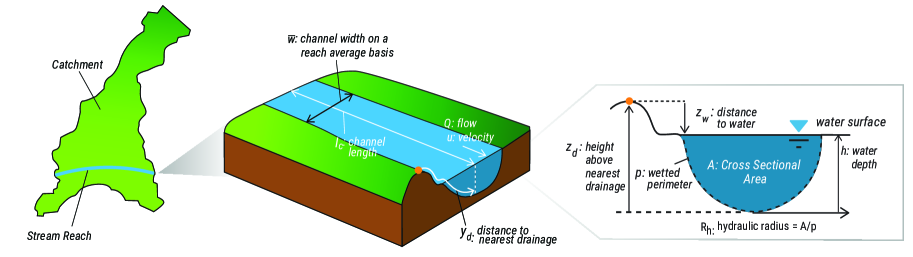
Figure 1: The governing parameters for the flow hydraulics, where at a point, flooding occurs when the distance to water is less than or equal to zero.

For a flood event, equations (1) and (2) determine the maximum water surface depth $h_{\max}$. Any given point is floooded when $h_{\max}$ exceeds the elevation above nearest drainage, $z_{d}$ (Fig. 1). The difference, $h_{\max}-z_{d}$, is the distance to water, $z_{w}$, where a point is flooded when $z_{w}\leq 0$ (Fig. 1). We assume $z_{w}$ is dependent on the following:

1. $Q$ [L³/T], the flow rate, for the flood magnitude constraint,

2. $z_{d}$ [L], the height above the nearest drainage, for constraining the number of flooded points,

3. $K_{v}$ [L/T], the velocity of conveyance (i.e., $K/A$) of flow representing the channel capacity constraint,

4. $A$ [L²], the channel cross sectional area,

5. $gS_{0}$ [L/T²], the slope multiplied by gravity, representing the external force driving the flow downslope.

The velocity, $u_{c}$, and friction slope, $S_{f}$, are not considered as they are derived directly from the listed variables. Furthermore, we are not considering time because flooding is based on the maximum flow and water level height, $Q_{\max}$ and $h_{\max}$, respectively. Hence, the water depth, $z_{w}$, is considered to be the maximum water level during a flood event.

Based on the Saint-Venant equations and the assumed channel geometry, the distance to water is a function of 5 variables, i.e., $z_{w}$ = $f(Q,K_{v},z_{d},A,gS_{0})$, and two dimensions, i.e., length [L] and time [T]. Following Buckingham $\Pi$ theorem, the required number of $\pi$ groups is $6-2=4$, where we have 1 dependent and 5 independent variables. The $\pi$ groups based on the two repeating variables, $K_{v}$ and $A$, are

$$\pi_{1} =\frac{z_{w}}{\sqrt{A}},$$ (4)

$$\pi_{2} =\frac{Q}{K_{v}A},$$ (5)

$$\pi_{3} =\frac{z_{d}}{\sqrt{A}},$$ (6)

$$\pi_{4} =\frac{gS_{0}\sqrt{A}}{K_{v}^{2}},$$ (7)

where the groupings were selected by inspection. This process yields the following dimensionless $\pi$ group relationship:

$$\pi_{1}=f(\pi_{2},\pi_{3},\pi_{4}),$$ (8)

where $\pi_{1}$, the distance to the flood surface, $z_{w}$, normalized by the square root of the channel cross sectional area, $\sqrt{A}$, is a function of the other terms, $\pi_{2}$, $\pi_{3}$, and $\pi_{4}$. The term $\pi_{2}$ represents the ratio of flow to flow capacity, $\pi_{3}$ accounts for how channel geometry (e.g., channel expansion and contraction) impacts flooding, while $\pi_{4}$ represents the flow velocity constrained by the gravitational force over the flow velocity constrained by the frictional force. Note that $\pi_{3}$ does not exist without reference to a stream or river for defining the height above the nearest drainage, $z_{d}$.

II.2 Hydrology

To identify flooding over typically wet areas with a saturated soil, we consider the assumptions of TOPModel (Beven, 2012) where the water table dynamics (from the surface) are considered as a secession of steady states that balance the long term watershed recharge with outflow from the saturated soil layer. Accordingly, the long term recharge (per unit contour length) is given by

$$q_{r} =a_{l}r,$$ (9)

where $q_{r}$ is recharge flow rate (per unit contour length), $a_{l}$ is the contributing area (per unit contour length), and $r$ is the uniform recharge rate (per unit area); see Figure 2. Note $a_{l}$ is equal to the contributing area, $a_{c}$. In steady state, $q_{r}$ is balanced by the outflow governed by Darcy’s law with the hydraulic gradient, $dh/dx$, approximated by the local topographic slope, $S$ Beven (2012), and a hydraulic conductivity that deceases exponentially with the soil depth, i.e.,

$$k_{s}\int_{z_{g}}^{\infty}e^{-\frac{z}{z_{d}}}dz =k_{s}z_{d}e^{-\frac{z_{g}}{z_{d}}},$$ (10)

where $k_{s}$ is the saturated hydraulic conductivity at the surface that decreases exponentially with a decay factor of $1/z_{d}$ (Ducharne, 2009), and $z$ is depth from surface (Fig. 3). Different from TOPModel, we have assumed the decay factor is the reciprocal of the height above nearest drainage for a point. Consequently, the average hydraulic conductivity occurs at the elevation of the nearest drainage flow path. Accordingly, the water table outflow (per unit contour length) is

$$q_{o} =Sk_{s}z_{d}e^{-\frac{z_{g}}{z_{d}}},$$ (11)

where $q_{0}$ is the (per unit contour length) outflow.

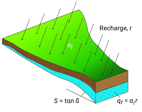
Figure 2: Following TOPModel, the moisture recharge flow per unit contour length, $q_{r}$, is the spatially uniform recharge rate (per unit area), $r$, multiplied by the contributing area per unit contour length, $a_{l}$, and the groundwater table parallels the topographic slope, $S$.

In steady state, the inflow of Eq. (9) equals the outflow of Eq. (11), i.e., $a_{l}r=Sk_{s}z_{d}e^{-\frac{z_{g}}{z_{d}}}$, and after rearranging terms, we retrieve the relationship between two dimensionless terms,

$$\frac{z_{g}}{z_{d}}=-\ln\left[\frac{a_{l}\ r}{z_{d}k_{s}S}\right],$$ (12)

where the depth to groundwater, $z_{g}$, normalized by the height above drainage, $z_{d}$, is equivalent to the natural log of the recharge inflow normalized by the outflow of Darcy’s law with the hydraulic gradient subsumed by the topographic slope, $S$, over a depth equal to the height above nearest drainage (per unit contour length) (Fig. 3).

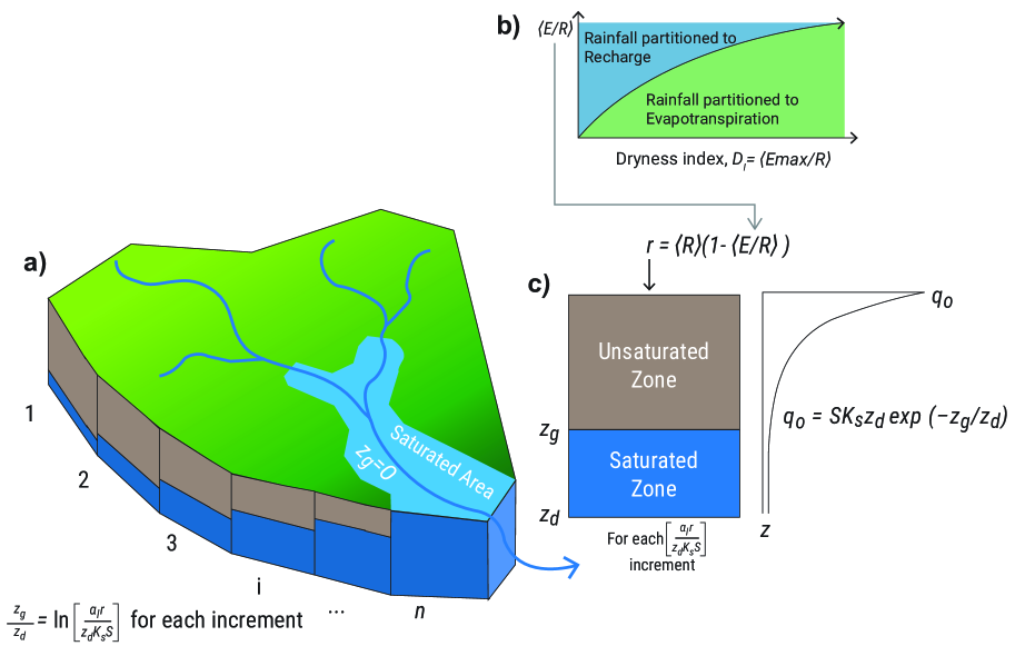
Figure 3: The watershed hydrology for calculating wet saturated areas (prone to flooding) is based on a) the TOPModel assumption of a spatially variable inflow rate derived from the contributing area (per unit contour length), $a_{l}$, multiplied by the watershed recharge rate, $r$, here derived from b) a partition of rainfall to evapotranspiration, $\langle E/R\rangle$, given by the Budyko curve (defined as $\langle E/R\rangle=\{D_{I}[1-\exp(-D_{I})\tanh(1/D_{I})]\}^{0.5}$ (Rodríguez-Iturbe and Porporato, 2004)), that is balanced by c) a water table that parallels the surface slope with soil water lateral transmission, $q_{o}$, that decreases exponentially with depth.

Based on Eq. (12), the distance to the groundwater surface, $z_{g}=f(z_{d},q_{r},q_{d})$, is dependent on (Smith et al., 1987)

1. $z_{d}$ [L], the height above drainage, for constraining the number of flooded points,

2. $q_{r}$ [L²/T], the moisture recharge flux into a point per unit contour length,

3. $q_{d}$ [L/T], the groundwater flux based on Darcy’s law, i.e., $k_{s}S$, assuming the hydraulic gradient, $dh/dx$, is represented by the topographic surface slope, $S$.

Hence, the system consists of 4 variables and 2 dimensions, so the Buckingham $\Pi$ theorem yields two $\Pi$ groups ($4-2=2$). From Eq. (12), these $\Pi$ groups are

$$\Pi_{1} =\frac{z_{g}}{z_{d}},$$ (13)

$$\Pi_{2} =\frac{a_{l}\ r}{z_{d}\ k_{s}\ S},$$ (14)

where we have substituted $q_{r}$ with $a_{l}r$ from Eq. (9) and $q_{d}$ with $k_{s}S$ following the assumption of TOPModel. These $\Pi$ groups provide for the following dimensionless relationship:

$$\Pi_{1}=\ln(\Pi_{2}),$$ (15)

where the natural log function is inferred from inspection of Eq. (12). The term $\ln(\Pi_{2})$ is akin to the topographic wetness index (Beven and Kirkby, 1979); but, differently, the argument of the natural log function, $\Pi_{2}$, is dimensionless and reflects ratio of water accumulation to water outflow from groundwater (per unit countour length).

II.3 From Buckingham $\Pi$ theorem to ML

Following the Buckingham $\Pi$ theorem, flooding is determined by the dimensionless groups $\pi_{1}$ or $\Pi_{1}$ for flooding from channel flow path expansion and in saturated areas (i.e., lakes and depressions), respectively. In both cases, when either $\pi_{1}$ or $\Pi_{1}$ is negative, an area is flooded but when both $\pi_{1}$ and $\Pi_{1}$ are positive an area is not flooded. Thus, the binary result of flooded (e.g., 1) and not flooded (e.g., 0) is found by applying a multidimensional Heaviside function, $\Theta(\cdot,\cdot)$, i.e.,

$$1-\Theta(\Pi_{1},\pi_{1})=1-\Theta[f(\pi_{2},\pi_{3},\pi_{4}),\ln(\Pi_{2})],$$ (16)

for which the Heaviside step function is only 1 if both arguments are positive, the function is right continuous, i.e., $\Theta(0,0)=1$, and the function $f(\pi_{2},\pi_{3},\pi_{4})$ is unknown. Here, we consider that a ML algorithm may subsume the overall function $\Theta(f(\pi_{2},\pi_{3},\pi_{4}),\ln(\Pi_{2}))$. Specifically, we consider the logistic regression for the likelihood (probability of flooding), i.e.,

$$1-\Theta(\Pi_{1},\pi_{1})\approx\Theta[P(\ln[\pi_{2}],\ln[\pi_{3}],\ln[\pi_{4}],\ln[\Pi_{2}])-\epsilon)],$$ (17)

where $P(\ln[\pi_{2}],\ln[\pi_{3}],\ln[\pi_{4}],\ln[\Pi_{2}])$ is the logistic regression probability, the natural log, $\ln[\cdot]$, is applied to all terms because we assume a multiplicative relationship (i.e., addition in log space results in multiplication of the variales), and the discrimination threshold, $\epsilon$, allows for the step function, $\Theta(\cdot)$, to filter the logistic regression probability into flooded (i.e., 1) or not flooded areas (i.e., 0).

Table 2: Data Sources

Data Type	Source	Download URL
Digital Elevation Model (DEM)	USGS Elevation Products (3DEP)	https://apps.nationalmap.gov
Land Use	National Land Cover Database	https://www.mrlc.gov/
Soil Type	NRCSa SSURGO from NRCS	https://www.nrcs.usda.gov/wps/portal/nrcs/main/soils
Hydrography	National Hydrography Dataset (NHD)	https://apps.nationalmap.gov
Watershed Boundaries	USGS Hydrologic Units (HU)	https://apps.nationalmap.gov
Flood Maps	FEMA Risk MAP Program	https://msc.fema.gov/portal/home
Climatology	Daymet	https://daymet.ornl.gov/

^a NRCS is the Natural Resources Conservation Service

III Processing of the Dimensionless Indices

The $\pi$ and $\Pi$ group indices are derived from the values of $a_{l}$, $r$, $z_{d}$, $S$, $S_{o}$, $A$, $R_{h}$, $n$, and $K_{v}$ (Table 1) that are calculated from the raw data of Table 2, which includes digital elevation models (DEMs), land use, soil type, hydrography, watershed boundaries, and climatology, and flood maps. Processing of the raw data is performed using GRASS GIS (Jasiewicz and Metz, 2011). For watersheds in the United States defined by a 12-digit United States Geological Survey (USGS) hydrologic unit code (HUC), the initial data processing steps consists of 1) downloading the relevant data of Table 2, 2) clipping the data to a buffered area around the desired watershed, and 3) hydro-enforcing (i.e., ‘burning‘) the DEM with the stream and river hydrography centerlines. Each HUC 12 watershed is around 100 km² on average and has a corresponding flood extents and hydrology given by the FEMA database listed in Table 2. The data processing first involves transforming the raw data into hydrologic and hydraulic attributes at each point in the watershed.

III.1 Properties at each point

At each point, we calculate the recharge, $r$ (which relates to the watershed climatology), the local topographic slope $S$, the Manning’s roughness coefficient, $n$, the saturated hydraulic conductivity, $k_{s}$, the overland flow velocity, $u$, and the contributing area (for flow), $a_{c}$. For each point, the contributing area of flow, $a_{c}$, (based on the DEM flow direction) is calculated using r.watershed in GRASS GIS (Jasiewicz and Metz, 2011). Over the hydroenforced DEM, the GRASS GIS r.watershed routine calculates the drainage direction and accumulation of grid cells. The accumulation of grid cells is converted to contributing area, $a_{c}$, based on the DEM resolution. Note that the value of the contributing area per unit contour length, $a_{l}$, is equal to the contributing area, $a_{c}$. Most GIS based values are calculated with GRASS GIS (Jasiewicz and Metz, 2011) including the slope at each point, $S$, as well as the roughness coefficient, $n$, based on the land use data (Chow, 1959). Values for the saturated hydraulic conductivity, $k_{s}$, were extracted from the Soil Survey Geographic Database (SSURGO) database and are representative values for the most restrictive soil component (e.g. lowest $k_{s}$ value) in the top five meters.

Climate variables are extracted from the Daymet dataset (Table 2). Annual averages of potential evapotranspiration, $\langle E_{\max}\rangle$, and precipitation, $\langle R\rangle$ are used to define a dryness index $D_{I}=\langle ET_{\max}/R\rangle$. In turn, the dryness index, $D_{I}$, is used with the Budyko curve (defined as $\langle E/R\rangle=\{D_{I}[1-\exp(-D_{I})\tanh(1/D_{I})]\}^{0.5}$ (Rodríguez-Iturbe and Porporato, 2004)) to calculate the rainfall partitioned to evapotranspiration, i.e., $\langle E/R\rangle$ and to runoff, i.e., 1- $\langle E/R\rangle$. Note that this runoff partition includes both the fast surface runoff, as well as the runoff through baseflow. Further, refinement could estimate the baseflow component alone. Finally, the long-term recharge rate is approximated as $r=\langle R\rangle(1-\langle E/R\rangle)$.

For each point, we calculate the conveyance velocity, $K_{v}$, which is the conveyance, $K$, divided by the flow cross-sectional area, $A$. This conveyance velocity at a point, $K_{v}$, is the average of $\frac{1}{n}R_{h}^{2/3}$ (based on Manning’s equation) over all points tributary to a point, multiplied by $\frac{a_{c}^{1/2}}{\overline{a_{c}^{1/2}S^{1/2}}}$, which accounts for the hydraulic radius, $R_{h}$, scaling with the flow convergence, $a_{c}$, normalized by $\overline{a_{c}^{1/2}S^{1/2}}$, which is an average over all points tributary to a point (Maidment et al., 1996). The conveyance velocity calculation follows the velocity calculation for the geomorphological instantaneous unit hydrograph (GIUH) (see Appendix C) for estimating the peak flow for all points over the watershed.

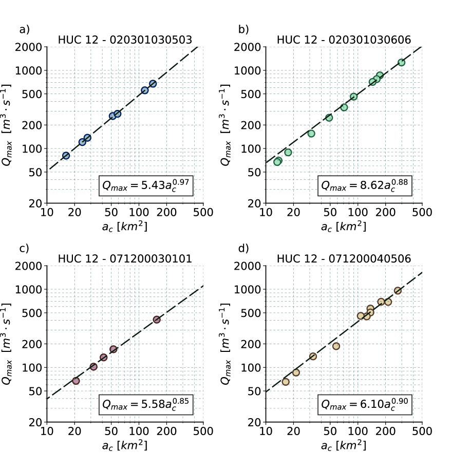
Figure 4: The relationship of peak flow, $Q_{max}$, to contributing area, $a_{c}$. The relationship is based on a series of geomorphological instantaneous unit hydrographs (calculated for each watershed) and a runoff hyetograph based on the NOAA Atlas 14, 100-year rainfall event (Table 4), a rainfall hyetograph given by the 2nd quartile, 50th decile of the NOAA Atlas 14, and runoff calculated with the NRCS-CN method (Table 4).

III.2 Peak flow model

The peak flow feature, $Q$, is derived (for any watershed point) from the effective precipitation (i.e., runoff) hyetograph, $p(\cdot)$, convolved over the instantaneous unit hydrograph (IUH), $f_{h}(\cdot)$, i.e.,

$$Q=\max\left[a_{c}\int_{0}^{t}f_{h}(t-\tau)p(\tau)d\tau\right],$$ (18)

where $Q$ is the maximum flow rate, $a_{c}$ is the (contributing) area of watershed, and $\tau$ is the time from the beginning of the storm. The IUH may be represented by simple conceptual approaches (Nash, 1957), or through a geomorphological theory. Here, geomorphological theory is used to derive the IUH, $f_{h}(t)$, consistent with the Saint-Venant equations considered over the local topography and land use data (see Appendix C).

For any effective precipitation hyetograph, the peak flow is defined through Eq. (18). In turn, the maximum flow roughly may be inferred as function of the contributing area (Nardi et al., 2006; Rigon et al., 2011), i.e.,

$$Q=c_{1}\left(a_{c}\right)^{c_{2}}$$ (19)

where $c_{1}$ and $c_{2}$ are found by fitting the equation to multiple (watershed specific) data points derived from the area and flow relationship of Eq. 18 (Fig. 4).

Accordingly, for each HUC 12 watershed, we divide the watershed into a series of nested watersheds down to an area of around 10 km², and we calculate a series of data points relating contributing area to the maximum flow. Subsequently, we find the parameters $c_{1}$ and $c_{2}$ from the best fit line, and then map the contributing area to the peak flow based on Eq. (19) (Rigon et al., 2011). Generally, a log-linear relationship well describes how the peak flow scales with the contributing area for each HUC 12 watershed (Fig. 4).

III.3 Channel properties and geometry

Modeling of channel proprieties begins with the delineation of the stream and river network. From the point properties, we have defined the accumulation of cells based on the drainage direction over the hydro-enforced DEM. From the flow accumulation and the hydro-enforced DEM, we then extract the stream raster with the GRASS GIS routine r.stream.extract that is given a threshold of cells for defining a stream. Here, we use two thresholds for a local and nonlocal delineation of the flow paths where the local threshold defines the more localized smaller drainage paths, while the nonlocal threshold delineates the major streams and rivers. We use the same thresholds across all watershed types to produce the data on a consistent basis. This consistency provides for reproducibility of the process. We assume the extracted flow paths represent the centerlines of channelized flow.

With the channel centerlines defined at two different scales for local flow paths (e.g., streets) and nonlocal flow paths (e.g., major streams and rivers), we then assume the channel roughness coefficient, $n$, and slope $S_{o}$ are based on the values at the channel centerline (for the respective scale of delineation). The slope at the channel centerline is based on multiplying the stream raster by the local (point) slope raster (to retrieve slope along the channel centerlines) and then averaging the centerline slope over a kernel of 5 grid cells using the GRASS GIS routine r.neighbors. For each channel centerline, the average slope, $S_{o}$, roughness coefficient, $n$, and flow accumulation, $a_{c}$, are mapped to points along the assumed cross-section of the channel by using the GRASS GIS routine r.stream.distance. This mapping links points (along the channel cross section) to the stream centerline based on the drainage direction raster (see Fig. 5). For mapping with r.stream.distance, all values (e.g., accumulation, roughness, and slope) not overlapping the stream centerline are converted to zero. At each point, r.stream.distance subtracts the centerline value (of accumulation, slope, etc.) from the zero value at each point. Subsequently, negative values are made positive and zero values are reverted back to the original values. This results in the centerline value being mapped to the points around the centerline (see Fig. 5). In addition, we use also use r.stream.distance with the original DEM and the drainage direction raster to extract the height above the nearest drainage (HAND), $z_{d}$, and distance from the nearest drainage (DFND), $y_{d}$. See Figure 5.

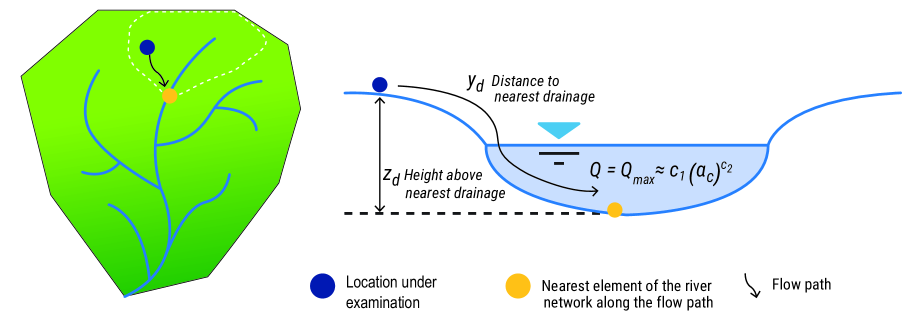
Figure 5: For each flow path centerline, the cross section is based on the drainage flow path to the centerline. Values from the flow-path centerline are mapped (following the drainage direction) to the points along the cross section. The contributing area of the flowpath is at the centerline and these value are converted to flow based on Eq. (19) and in turn mapped to the adjacent cross section points.

The channel cross sectional area and hydraulic radius vary around the reach average values. Accordingly, we calculate the reach average values and then vary the point values around the reach average value. The reach average values are based on an incrementally increasing water depth, $z_{w}$ (Fig. 1), and calculating the water surface area of flooding, $A_{s}$, the channel bed area, $\overline{A}_{b}$, the volume of water in the inundated area, $\overline{V}$, the reach average channel width, $\overline{w}=A_{s}/l_{c}$, where $l_{c}$ is the channel reach length, the reach average cross sectional area, $\overline{A}_{c}=\overline{V}/l_{c}$, and the reach average hydraulic radius, $\overline{R}_{h}=\overline{A}_{c}/(\overline{A}_{b}/l_{c})$, where $\overline{A}_{b}/l_{c}$ is the reach average wetted perimeter (Zheng et al., 2018b; Garousi-Nejad et al., 2019).

At any point in the watershed, the specific channel cross sectional area, $A$, and hydraulic radius, $R_{h}$, are calculated from the reach average values as

$$A =\alpha_{A}\overline{A}_{c},$$ (20)

$$R_{h} =\alpha_{R_{h}}\overline{R}_{h},$$ (21)

where the factors $\alpha_{A}$ and $\alpha_{R_{h}}$ are calculated from the height and distance from drainage values. The factor $\alpha_{A}$ for adjusting the cross sectional area is given by

$$\alpha_{A}=\frac{2y_{d}}{\overline{w}},$$ (22)

which is the ratio of river width (estimated as $2\cdot y_{d}$) to the reach average width, $\overline{w}$. The factor for adjusting the hydraulic radius, $\alpha_{R_{h}}$, is based on both $\alpha_{A}$, and a factor for the wetted perimeter assuming the cross sectional area is approximated by a triangular or parabolic cross section (Appendix B). In turn, the conveyance velocity is calculated at each point as $K_{v}=\frac{1}{n}R_{h}^{2/3}$ where the Manning’s roughness coefficients have been mapped from the nearest stream. Note that the hydraulic radius, $R_{h}$, and cross sectional area, $A$, are defined based on a cross section originating from each point following the flow path to the nearest drainage.

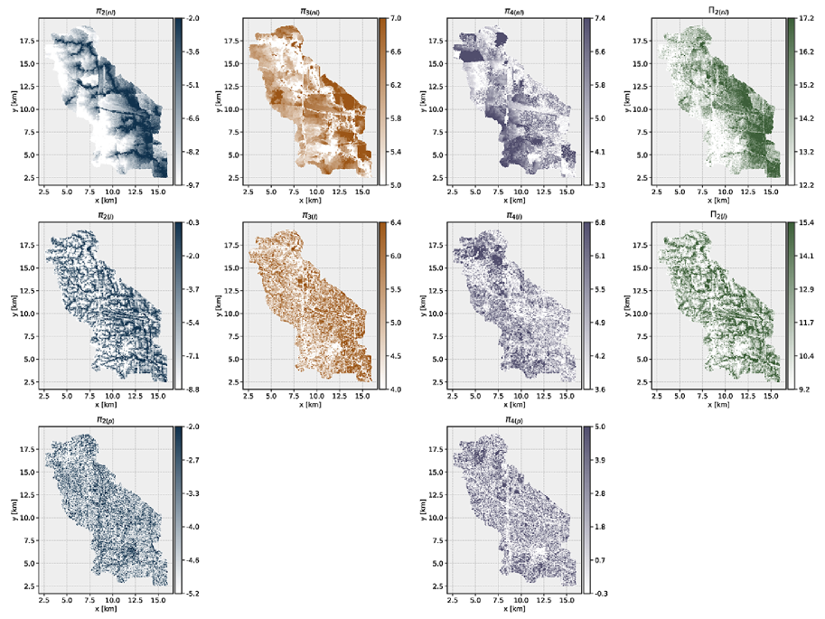
Figure 6: For HUC 071200040403, the dimensionless indices at the different scales of 1) the nonlocal, major streams and rivers with a contributing area greater than 1 sq. mile, i.e., $\pi_{2(nl)}$, $\pi_{3(nl)}$, $\pi_{4(nl)}$, and $\Pi_{2(nl)}$, 2) the localized flow paths (e.g., streets) with a contributing area greater than 0.01 sq. mile, i.e., $\pi_{2(l)}$, $\pi_{3(l)}$, $\pi_{4(l)}$, and $\Pi_{2(l)}$, and at each point, i.e., $\pi_{2(p)}$ and $\pi_{4(p)}$. The $\pi_{2}$ terms are based on flow $Q$ derived from the NOAA Atlas 100-year rainfall event (Table 4), the 2nd quartile, 50th decile of the NOAA Atlas 14 precipitation hyetograph, and the NRCS-CN method for transforming rainfall (see Table 4).

III.4 Indices at different scales

The dimensionless indices $\pi_{2}$, $\pi_{3}$, $\pi_{4}$, and $\Pi_{2}$ are calculated at different scales: 1) at each point, i.e., $\pi_{2(p)}$ and $\pi_{4(p)}$, 2) in relation to localized flow paths (e.g., streets), i.e., $\pi_{2(l)}$, $\pi_{3(l)}$, $\pi_{4(l)}$, and $\Pi_{2(l)}$, and 3) in relation to major streams and rivers that may create a non-localized flooding, i.e., $\pi_{2(nl)}$, $\pi_{3(nl)}$, $\pi_{4(nl)}$, and $\Pi_{2(nl)}$, where $\pi_{3}$ and $\Pi_{2}$ do not exist at a point because the height above drainage is non-existent without reference to a stream (Fig. 6). At a point, $\pi_{2(p)}$ and $\pi_{4(p)}$ are based off of the point values of the variables $Q$, $A$, $k_{v}$, and $S_{o}$, where the channel slope, $S_{o}$ is the local slope, $S$, the cross sectional area $A$ is based on sheet flow depth over a unit width, and $K_{v}$ is the point value; see Section (III.1). We are consistent in generating the indices based off of one constant value of sheet flow depth (as discussed in Section V); however, in the future this could be linked to the intensity of the precipitation event.

The local ($\pi_{2(l)}$, $\pi_{3(l)}$, $\pi_{4(l)}$, $\Pi_{2(l)}$) and nonlocal ($\pi_{2(nl)}$, $\pi_{3(nl)}$, $\pi_{4(nl)}$, $\Pi_{2(nl)}$) indices (based on Eqs. (4) to (7)) are in relation to the channel flow path delineation. The flowpath delineation determines the height above nearest drainage, $z_{d}$, as well as the values of the slope, $S_{o}$, and the roughness coefficient, $n$, which are mapped from the flow path centerline to the surrounding points. In addition, the channel flow paths determine the reach length, $l_{c}$, for the reach average hydraulics that in turn affect the final values of the cross sectional area and the hydraulic radius. Note that the conveyance velocity, $K_{v}$, is not based on assumption for the point value, but is calculated directly from the properties at the channel centerline, i.e., $K_{v}=\frac{1}{n}R_{h}^{2/3}$. The dimensionless indices (at the different scales) have a low correlation, but some of the local and nonlocal features and hydraulic and hydrologic features have a stronger correlation; see Appendix D. The low correlations shown by the indices make them well suited for an ML application (Murphy, 2022).

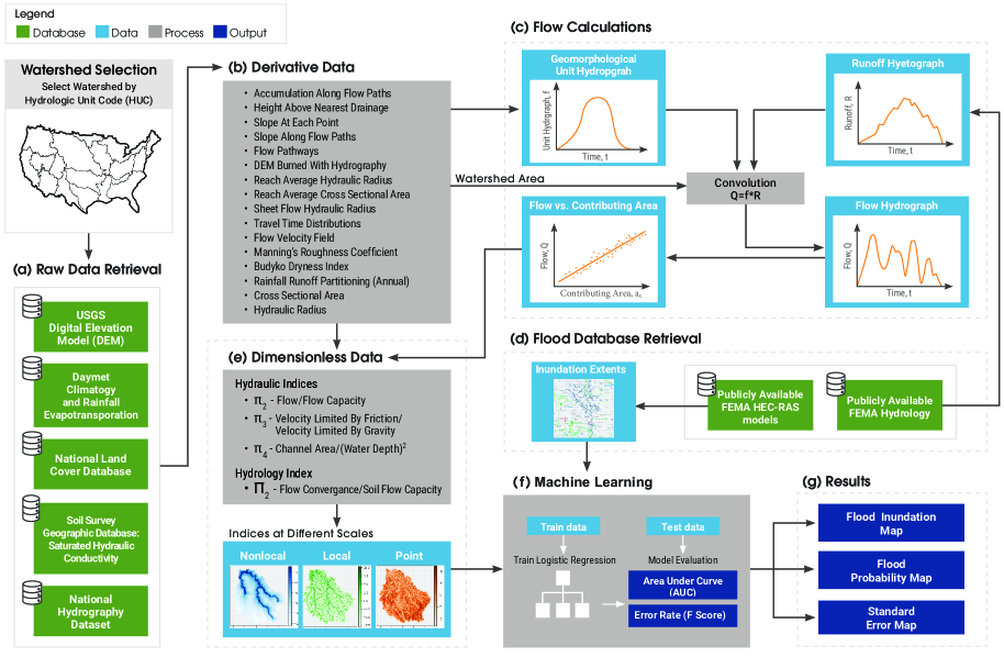
Figure 7: The ML process is constructed for selected HUC 12 watersheds across the United States. For each selected HUC 12 watershed, a) the raw data is retrieved, b) the raw data is processed into derivative data, c) the flood hydrology and extents are downloaded, d) the derivative data and flood hydrology are used to construct a series of geomorphological instantaneous unit hydrographs to relate the peak (maximum) flow to contributing area, e) the flow and derivative data are combined into dimensionless indices that capture the hydraulic and hydrologic similarity of the flooding process, f) the dimensionless data is related to the flood extents by an ML logistic regression model, and g) the logistic regression model produces flood extents, flood probability, and the error in comparison to the original training data.

IV Machine Learning Methodology

The ML algorithm mapped the $\pi_{2}$, $\pi_{3}$, $\pi_{4}$ and $\Pi_{2}$ indices (at different scales) to an output (flood extents) that matched the ground truth (HEC-RAS based flood maps) as faithfully as possible (Hastie et al., 2009). The overall ML process (Fig. 7) consisted of the following steps of 1) dimensionless feature creation and data validation, 2) model development and training, and 3) model deployment and monitoring.

IV.1 Pluvial flooding ground-truth (label) data

The ground-truth observations used for the ML training were taken from HEC-RAS models that were run with a spatially uniform runoff hyetograph applied over a 2D area. These HEC-RAS model results for pluvial flooding were from the FEMA inventory. FEMA manages an existing inventory of stream studies that includes approximately 1.2M miles of fluvial stream studies (Government Accountability Office, 2021). This inventory, though it carries an industry leading standard of care (Wing et al., 2017), is limited in capturing local pluvial hazard risks (Government Accountability Office, 2021). However, since 2019, FEMA has begun to expand the flood hazard data developed per model by including HEC-RAS 2D models with runoff applied over a 2D watershed area. These 2D results provide for a more detailed probabilistic flood risk analyses, and with these models FEMA is moving towards developing more graduated flood risk data nationwide (Technical Mapping Advisory Council, 2020). In this study, we benchmarked the ML training and validation using available FEMA rainfall/runoff input and flood hazard output data from two-dimensional HEC-RAS models.

IV.2 Feature creation, data validation, and model training

In the dimensionless feature creation and data validation step, we checked the raw data quality (e.g., missing values, resolution, etc.), and if the data is of sufficient quality, we processed the raw data into the dimensionless indices (Fig. 7). In turn, the dimensionless indices were stored in a database that was validated for reasonable values of the indices. Furthermore, for model training, we only used data that overlaped with a HEC-RAS 2D model flood maps, which still resulted in trillions of data points for the model development.

The features (i.e., the dimensionless indices) were stored as a tabular dataset where each row (corresponding to one grid area within the watershed) contained multiple columns, with columns respectively containing either the dimensionless features, the geographic location of that grid, or the identification information, e.g., the HUC 12 code. To keep track of feature improvements, the tabular dataset was stored with a versioning system that allowed the data to be rolled back to an earlier version. This versioning provided data provenance and lineage, so model training and performance were tracked and evaluated within the context of the dimensionless features.

Before ML model training, the stored features were validated to confirm stored data matches requirements including but not limited to type, e.g., integers, domain, and values e.g., positive values only for flows, and missing values. These validation steps limited the ML model to a sufficient data quality needed for efficiently training models that provide high quality predictions of flooding. If a feature dataset did not meet the pre-defined requirements, it was rejected and not used for model training. Once the engineered features were computed for the training data, stored, and validated, model development and training on that data can proceed.

Two regions were used for model training and testing, namely four watersheds in the Chicago area (with HUC 12 codes starting with 0712), and four watersheds in New Jersey (with HUC 12 codes starting with 0203). Two combinations of these watersheds were considered for training to evaluate the predictive performance and general applicability of the models across regions (see Table 3). Since there was a spatial dependency of the points in the data, the train-test splits were performed such that entire watersheds were either included or held out from training. In Case 1, all watersheds from the Chicago region were used for training, and each of the four watersheds in New Jersey were used for testing (approximately 50%-50% train-test split). In Case 2, one watershed from Chicago and one from New Jersey are held-out for testing, with the remaining six watersheds used for training (approximately 60%-20% train-test split).

For the ML model, we used logistic regression because its simplicity demonstrated how the indices captured the similarity of flooding across different regions. The inputs to the logistic regression were the dimensionless indices (and not derivative values found from a polynomial expansion). In addition, as mentioned for Eq. (17), we inputted the natural log of the indices into the logistic regression. This logistic regression model was trained to maximize the performance of the algorithm in matching the ground truth data (HEC-RAS based flood maps) (Murphy, 2022). A best match was found by adjusting weights applied to each dimensionless feature (see Appendix E), and in a further step a best fit was achieved by optimizing the probability threshold used to classify points as flooded (class 1) or not flooded (class 0). In turn, the optimal threshold threshold then was used to classify points within the test watersheds. Finally, we deployed the logistic regression model as a service that may be queried for flood extents (given a new hydrology or both a new hydrology and watershed area).

Performance was based on the receiving operator characteristic (ROC) curve of which the performance is often summarized as an area under curve (AUC). We used the ROC and AUC to assess performance because ROC curves are insensitive to class imbalance (Murphy, 2022), which may vary significantly for flooding over different event severities (e.g., 10-year, 100-year return period events). We monitored the AUC of the model to evaluate its performance over different areas (to assess the need for model retraining or improvements). For reference, we also reported the F-score with the recall weighted as twice as important as the precision (i.e., $\beta=2$, see Appendix F); however, note that the differences in the F-score between events was primarily a result of the increasing class imbalance (i.e., there is less flooded area) as the event severity decreases from the 1000-year to the 10-year event.

Table 3: Case Study Performance by Return Period Event

Case I
ML Training	ML Testing	Test AUCa			Test F2-scoreb
HUC 12	HUC 12	10-yr.	100-yr	1000-yr.	10-yr.	100-yr.	1000-yr.
071200030101
071200040403
071200040505
071200040506
	020301030606	0.91	0.93	0.94	0.75	0.82	0.83
	020301030503	0.93	0.9	0.9	0.65	0.74	0.78
	020301030703	0.95	0.86	0.87	0.66	0.67	0.73
	020301030804	0.95	0.85	0.85	0.71	0.67	0.70
Case II
071200030101
071200040403
071200040505
	071200040506	0.88	0.86	0.85	0.56	0.74	0.78
020301030606
	020301030503	0.94	0.9	0.9	0.68	0.76	0.79
020301030703
020301030804

^a ROC curves are displayed in Figure (8).
^b For the F_β-score with $\beta=2$; see Appendix F.

V Application

To showcase how the dimensionless indices capture the similarity of flooding we consider two applications of this methodology 1) we train the ML model (logistic regression) on data from watersheds around the Chicago area (i.e., HUC 12 watersheds beginning with 0712) and then test the model predictive performance on test data from northern New Jersey (i.e., HUC 12 watersheds beginning with 0203) and 2) we train the ML model on a combination of the Chicago and New Jersey watersheds with one hold out watershed (from each region) for testing (see Table 3). The purpose is to demonstrate how an ML model from one region of the country captures the flooding from a completely different region as a result of the power of the dimensionless indices in capturing the similarity of the flood process. Towards this end, for each case considered, we have created three ML (logistic regression) models for the 10-year, 100-year, and 1000-year events, respectively. The performance of the ML model is based on its performance on the test watersheds as assessed by the ROC curve and AUC.

For the watersheds in the case studies (Table 3), the underlying ground-truth flood maps are extracted from HEC-RAS 2D models that were run with a 24-hour storm for the 10-year, 100-year, and 1000-year events with the hydrology of Table 4. More specifically, the HEC-RAS 2D model results for depth are converted to a binary inundation flood map (Fig. 7) that is used to either train the ML model or to validate the ML model for test watersheds (Table 3). The hydrology of Table 4 is the basis for the runoff hyetographs extracted from the HEC-RAS 2D models that in turn is used to calculate the peak flow for the dimensionless indices (Fig. 7). In addition, for the case studies, the dimensionless indices were created assuming thresholds of 0.01 mi² and 1 mi² for the local and nonlocal delineation of the flow paths from digital elevation maps at a 1/9th arc-second resolution (which was the best available resolution available from the USGS at the time of this study). For the generation of the conveyance velocity at a point, we assumed a sheet flow depth of 0.01 in calculating the hydraulic radius $R_{h}$ (see Section III.1).

Table 4: Watershed Hydrology^a

	Rainfall (inches)				Runoff (inches)
HUC 12	10-yr.	100-yr	1000-yr.	Curve Numberb	10-yr.	100-yr	1000-yr.
071200030101	3.9	6.01	8.86	76	1.66	3.39	5.94
071200040403	4.38	7.19	11.24	86	2.89	5.55	9.5
071200040505	4.26	6.83	10.33	86	2.78	5.2	8.6
071200040506	4.36	7.12	10.99	88	3.06	5.71	9.51
020301030606	5.20	8.58	13.35	84	3.45	6.65	11.31
020301030503	5.17	8.47	13.09	82	3.22	6.51	10.78
020301030703	5.04	8.38	13.16	79	2.84	5.86	10.43
020301030804	5.11	8.53	13.44	82	3.18	6.36	11.12

^a Analysis based on NOAA Atlas 14 precip. hyetograph for 2nd quartile, 50th decile event.
^b The rainfall runoff transformation is based on the NRCS-CN method with an initial abstraction ratio of 0.2.

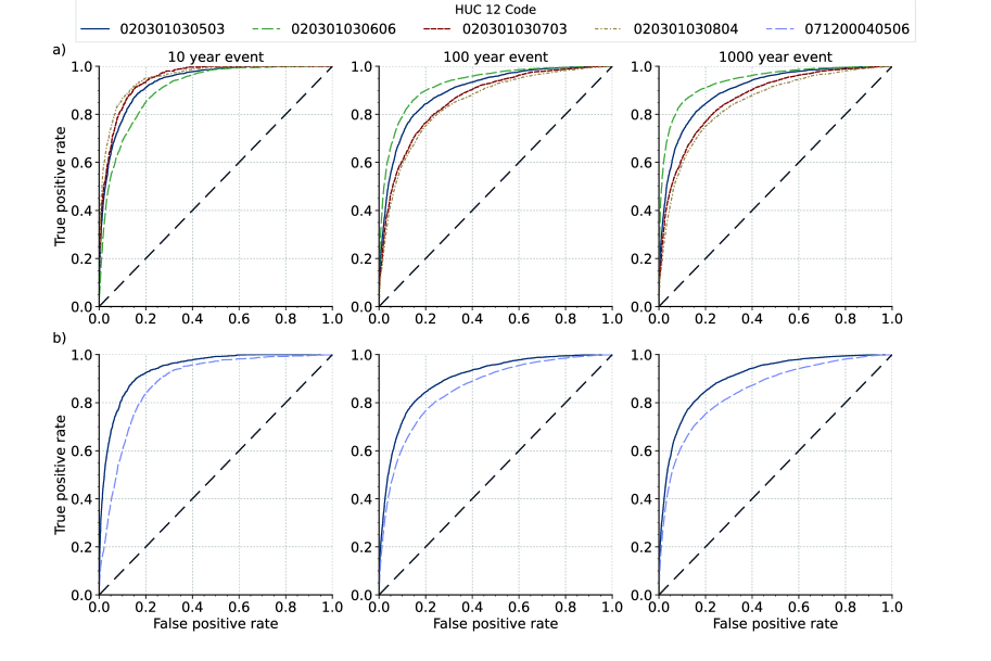
Figure 8: ROC curves for a) case I and b) case II of Table 3.

The ML model performs well based on the AUC scores of Table 3. Generally, an AUC score of 0.8 to 0.9 is considered excellent discrimination, while an AUC score greater than 0.9 is considered outstanding (Hosmer Jr et al., 2013). For reference, an AUC score of 0.5 provides no discrimination between flooded and non-flooded areas and is no better than a random guess. Across all events (e.g., 10-year, 100-year, and 1000-year), the average AUC scores are 0.9 and 0.89 for Cases I and II, respectively (Table 3). Categorically, the average AUC scores for the respective cases I and II are 0.93 and 0.91 for the 10-year event, 0.88 and 0.88 for the 100-year event, and 0.89 and 0.88 for the 1000-year event. Each of these AUC scores is associated with an ROC curve relating the trade-off between the ML model true positive rate and false positive rate (Fig. 8).

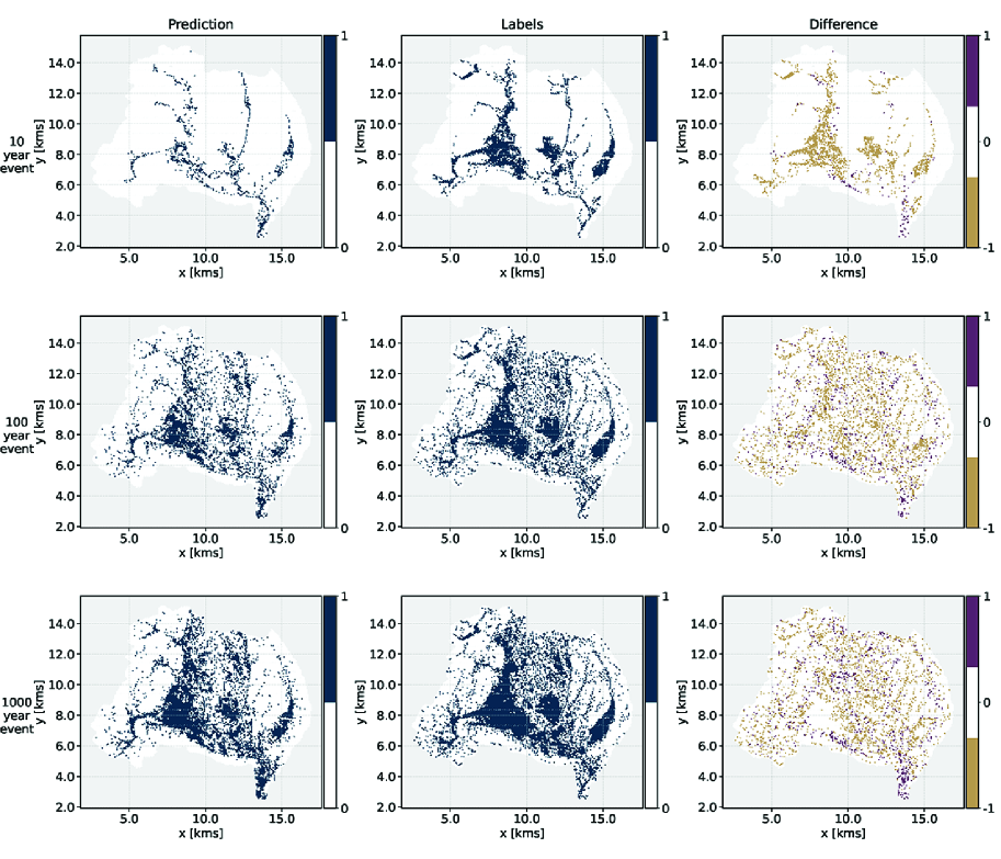
Figure 9: For the Case I test HUC 12 watershed of 020301030804, the ML predictions versus the HEC-RAS generated flood maps (labels) for different return period events, where the discrimination threshold (probability above which a point is flooded) for the 10-year, 1000-year, and 1000-year events are 0.822, 0.604, and 0.54, respectively.

For the test watersheds, Figs. 9 and 10 show the ML prediction of flooding in comparison to the ground-truth (labels) derived from HEC-RAS 2D inundation extents. Note that the ML logistic regression model outputs a probability distribution for the likelihood of flooding. This likelihood of flooding is evaluated at certain discrimination (probability) threshold, above which a point is mapped as flooded and below which a point is mapped as non-flooded. Accordingly, the ML model results may be tuned based on whether one desires a more conservative result that overpredicts potential flooding, or less conservative result that underpredicts potential flooding, but that is less likely to have false positives (i.e., predicting flooding where non should occur). For the given discrimination thresholds of Figs. 9 and 10, the ML model tends to underpredict the extents of flooding, though by lowering the discrimination threshold, these results could be reversed to a slight overprediction. Nevertheless, the ML model (logistic regression) generally captures the networked pattern of flash flooding as calculated by the HEC-RAS 2D models (i.e., the ground-truth labels of Figs. 9 and 10).

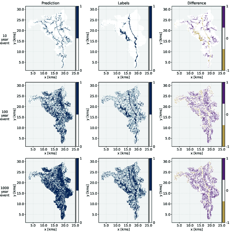
Figure 10: For the Case II test HUC 12 watershed of 071200040506, the ML predictions versus the HEC-RAS generated flood maps (labels) for different return period events, where the discrimination threshold (probability above which a point is flooded) for the 10-year, 1000-year, and 1000-year events are 0.832, 0.606, and 0.553, respectively.

For the discrimination thresholds shown in Figs. 9 and 10, the average F-scores for the test watersheds are 0.66, 0.74 and 0.77 for the 10-year, 100-year, and 1000-year events, respectively. The F-score is based on weighting the recall as twice as important as the precision (i.e., $\beta=2$ based on (Murphy, 2022, p. 171)); see Appendix F. The recall is weighted more heavily than precision because the goal is to assess the ability of the ML model to detect flooding while being less concerned with a more conservative answer with more false positives (that slightly overpredicts flooding). While the F-scores indicate that the ML model for the 10-year event could improve the most in performance, the lower F-score is primarily the result of the greater class imbalance for the 10-year event (i.e., there is much less flooded area in comparison to the non-flooded areas) (Murphy, 2022, see Eq. 5.31). It is evident that class imbalance impacts the F-score for the 10-year event because the ROC curves and AUC scores are relatively similar between the different events (Fig. 8). Generally, across all events, model performance would improve by detecting more of the flooded areas as shown by Figs. 9 and 10.

V.1 Discussion

The ML model predictions on the test watersheds (on which the model was not trained) produces test AUC scores of around 0.9 or greater. This result is comparable and exceeds previous ML model efforts that primarily focused on riverine flooding (e.g., Manfreda et al., 2014a; Samela et al., 2016). Differently, this work not only develop dimensionless indices, but also explores how these indices capture the similarity of the flooding process by allowing a simple ML model that is trained in one geographic region (i.e., Chicago) to capture flooding in a completely different geographic region (i.e., New Jersey). Moreover, to demonstrate the dimensionless indices potential in capturing the similarity of the flooding process, we used the logistic regression because it is simple and explainable. The logistic regression is a a one node, single layer neural network. Conversely, the multiple nodes and layers of a full neural network would make it difficult to assess the performance of the dimensionless indices in isolation of the ML model complexity. Furthermore, the indices alone are the inputs into the logistic regression, i.e.,there is no polynomial expansion of these indices, as is common in many ML applications.

The dimensionless indices when coupled to the ML model allow for a rapid prediction of pluvial (flash flood) extents. The processing of the dimensionless data takes about 2 hours for a DEM resolution of 1/9 arc-second (approximately 3-meter) and about 3 hours for a DEM resolution of 1-meter; however, this processing must only be done once. Once the derivative data (Fig. 7) is created, it is combined with new hydrology (i.e., runoff hyetographs) in seconds, and new ML results (based on new hydrology) are produced in minutes. Thus, with this ML approach, the runoff hyetographs from the latest weather forecasts (e.g., from the HRRR model) rapidly could be transformed into maps that inform flash flood warnings–a vast improvement on the current warnings that generally are given on a regional basis without specificity. This lack of specificity makes it difficult to truly understand the best actions for preserving life and maintaining safety during a flash flood warning.

Within the respective ML models for the 10-year, 100-year, and 1000-year events, there is a significant variation in the hydrology of the watersheds of around $\pm$ 1 inch (Table 4). Even though the hydrology varies, the ML models perform reasonably well because this hydrology is directly used to calculate the flow over the entire watershed. Flow is then embedded in the $\pi_{2}$ term. As we selected the logistic regression, all of the $\pi$ and $\Pi$ terms are weighted and added together to create a single sum that determines the logistic regression probability. Consequently, we needed three separate models in this study to cover a range of effective precipitation, as indexed by a return period. A decision tree based ML model could allow for one model where based on the $\pi_{2}$ term (that accounts for flow), the other terms could different thresholds for then discriminating flooded and non-flooded areas. In other words, the decision tree could partition the range of values for $\pi_{2}$ into several increments, where for each increment there are different thresholds for $\pi_{3}$, $\pi_{4}$ and $\Pi_{2}$ for determining flooding. Intuitively, the different decision points (for indices $\pi_{3}$, $\pi_{4}$ and $\Pi_{2}$) would reflect that the physical behavior of flooding is different for low flows versus high flow events.

While we have defined the dimensionless indices based on Buckingham $\Pi$ theorem, the definition of $\pi$ and $\Pi$ terms is not unique. Different formulations of the $\pi$ and $\Pi$ terms are equally valid under the Buckingham $\Pi$ theorem, and future work could explore and quantify how different formulations of the dimensionless indices relate to the similarity of the flooding process. Additionally, the processing of the data to create the $\pi$ and $\Pi$ terms could be improved, as here we performed a first attempt at creating the data to demonstrate the theory. Improvements, could include but are not limited to 1) better resolving the overall rate of groundwater recharge, $r$, 2) exploring the optimal thresholds for delineating flow paths at different scales for capturing the flood process (e.g., (Sangireddy et al., 2016)), 3) refining the estimated depth of sheet flow, which here was estimated as 0.01 meters globally (for example, the sheet flow depth could be related to the runoff hyetograph intensities), 4) refining the calculations for the channel cross sectional area and slope, and 5) resolving the reach average hydraulics at a subwatershed level within each HUC 12 watershed. Currently, the data processing calculates the reach average hydraulics for the entire HUC 12 watershed, and then varies the hydraulic attributes around these average hydraulics.

In this work, we have performed preliminary analysis of how changing the thresholds for delineating flow paths alters the performance of the logistic regression model. Specifically, we decreased the contributing area threshold for the nonlocal flow paths from 1 sq. mile to 0.2 sq. mile. The resulting performance change is in terms of the percent change in the F-score (Table 5). Generally, there is an overall performance decrease with the most significant performance decreases occurring for the 10-year event (Table 5). The 10-year event has the most dramatic performance decrease because most of the flooding for a 10-year event is centered around the major rivers and streams, and a lower nonlocal threshold (of 0.2 sq. miles) does not well define major rivers and streams. The significance of the change (Table 5 demonstrates that importance of optimizing the thresholds for flow path delineation in relation to ML model performance.

Though the similarity indices capture the likelihood of flooding in the Chicago area and in turn map flooding in northern New Jersey, further work is warranted in exploring this approach across a wide range of geographies and climate types. A detailed study could explore the similarity of flooding across different hydroclimatic and topographic regions. Potentially, in terms of ML model performance it could be advantageous to have ML models (based off of the dimensionless indices) that are specific to certain regions as characterized by generic climatic and topographic attributes (e.g., average slope). Additional work also could explore how the dimensionless indices could be expanded to capture riverine flooding and account for structures that control flooding, e.g., levees.

Some of the techniques from this study could improve the traditional regression analysis for estimating stream flow. Specifically, the geomorphological instantaneous unit hydrograph (GIUH) when convolved with a runoff hyetograph provides a watershed wide signature of the flow versus the contributing area (e.g., Fig. 4). With the GIUH relying on data that is readily available at a continental and even a world wide scale (e.g., DEM, landuse, etc.), it could be beneficial to integrate the GIUH attributes into the traditional regressiona analysis for streamflow (Capesius and Stephens, 2009). The performance of the ML model, which leverages the GIUH, shows that the GIUH has promise in estimating flow over regional areas. In particular, the log-linear relationship between contributing area and flow (Fig. 4) could be a factor in future regression analysis.

Table 5: Change in F-score with the nonlocal threshold (NL)

Case I - NL threshold decreased by 0.8 mi.2
ML Testing	Test F2-scoreb
HUC 12	10-yr.	100-yr.	1000-yr.
020301030606	-3.1%	0%	0%
020301030503	-3.6%	0%	-0.6%
020301030703	-10.1%	4.4%	-8.3%
020301030804	-8.1%	3.5%	-7.6%
Case II - NL Threshold decreased by 0.8 mi.2
071200040506	-9.5%	0%	0.6%
020301030503	-1%	-1.3%	-0.6%

^a ROC curves are displayed in Figure (8).
^b For the F_β-score with $\beta=2$; see Appendix F.

VI Concluding Remarks

By reformulating a physical problem into a dimensionless context with Buckingham $\Pi$ theorem, we may capture the similarity of a process (such as flooding and other natural hazards) across different environments and conditions. Through following Buckingham $\Pi$ theorem, we have formulated dimensionless indices that capture the similarity of the flash flood process, and we have calculated these indices from readily available raw data such as DEMs and land use maps. Future work could improve the methods for calculating these indices for capturing flood similarity. We have used these indices with a logistic regression ML model, and subsequently, have shown that over two different regions of the United States, the same values of these indices correspond to the a similiar likelihood of flooding, as defined by HEC-RAS 2D model runs. If the ML model is trained on actual observations (e.g., satellite), then an ML model prediction could be the basis for calibrating detailed hydraulic models such as HEC-RAS. Consequently, the logistic regression may use these indices to predict flooding in new areas and for new hydrology (i.e., forecast inputs). For a given weather forecast, this approach could provide the foundation for the rapid forecasting and mapping of pluvial flood hazard. Such a forecast of flood risk would involve mapping the dimensionless indices to flood hazard over a wide range of conditions. Accordingly future work will both examine how this approach scales across different regions and topographies, as well as adapting this approach to other flooding mechanisms such as riverine flooding and coastal flooding. We also anticipate that this approach will find general utility in assessing different geohazard risks.

Appendix A HEC-RAS 1D Standard Step

The Saint-Venant equations reduce down to the standard step approach of HEC-RAS 1D by assuming a steady state condition and integrating over the channel flow direction, $x$. In steady state, i.e, $\partial/\partial_{t}=0$, the continuity and momentum equations simplifies to

$$\frac{\partial Q}{\partial x} =0$$ (23)

$$\frac{1}{2}\frac{d(u_{c}^{2})}{dx} +g\frac{dh}{dx}+g(S_{f}-S)=0.$$ (24)

This steady-state momentum equation then may be integrated over the $x$ direction to retrieve

$$\frac{u_{c}^{2}}{2g}+h+(S_{f}+S_{0})\Delta x=Constant,$$ (25)

which is the Bernoulli equation that is the basis of the HEC-RAS 1D Standard Step solution for gradually varied flow (Chow, 1959, p. 267).

Appendix B Hydraulic Radius Adjustment factor

The hydraulic radius is the cross sectional area divided by the wetted perimeter. Accordingly, the factor adjusting the hydraulic radius, $\alpha_{R_{h}}$, is the factor for adjusting the cross sectional area, $\alpha_{A}$ (see Eq. (22)), multiplied by a factor for adjusting the wetter perimeter. Here, the wetted perimeter factor is a weighted combination of the factors for a triangular cross section, $\alpha_{T}$, and a parabolic cross section, $\alpha_{P}$, i.e.,

$$\alpha_{R_{h}}= \left\{\begin{array}[]{lll}\alpha_{T}\alpha_{A}&&A<A_{T}\\ \alpha_{T}\alpha_{A}\frac{A-A_{T}}{A_{P}-A_{T}}+\alpha_{P}\alpha_{A}\left(1-\frac{A-A_{T}}{A_{P}-A_{T}}\right)&A_{T}\leq&A<A_{P}\\ \alpha_{P}\alpha_{A}&A_{P}\leq&A\end{array}\right.$$ (29)

where the overall factor varies linearly depending on how the cross sectional area, $A$, compares to an assumed triangular cross section, $A_{T}=y_{d}\cdot z_{d}$, and parabolic cross section, $A_{P}=\frac{2}{3}2y_{d}\cdot z_{d}$–both calculated based on the distance from drainage, $y_{d}$, and height above drainage, $z_{d}$. The wetter perimeter factors for the triangular cross section, $\alpha_{T}$, and parabolic cross section, $\alpha_{P}$, respectively are (Chow, 1959)

$$\alpha_{T} =\frac{2z_{d}\sqrt{\frac{\overline{w}}{z_{d}}+1}}{2z_{d}\sqrt{\frac{2y_{d}}{z_{d}}+1}}$$ (30)

$$\alpha_{P} =\frac{\overline{w}+\frac{8z_{d}^{2}}{3\overline{w}}}{2y_{d}+\frac{8z_{d}^{2}}{3\cdot 2y_{d}}},$$ (31)

where the factor is the wetted perimeter based on the reach average width, $\overline{w}$, divided by the wetted perimeter based on the channel width (estimated as $2\cdot y_{d}$).

Appendix C Instantaneous Unit Hydrograph (IUH)

Following geomorophological theory, the IUH is consistent with both topography and the Saint-Venant equations without the inertial terms (assuming the Froude number is much smaller than 1) where the continuity and momentum equations have been merged into a diffusive wave equation Fan and Li (2006); Rigon et al. (2016), i.e.,

$$\frac{\partial Q(t,x)}{\partial t}+u_{c}\frac{\partial Q(t,x)}{\partial x}=D\frac{\partial^{2}Q(t,x)}{\partial t^{2}},$$ (32)

where $u_{c}$ is the channel velocity, and $D$ is a hydrodynamical diffusion coefficient. In accordance with Eq. (32), the IUH of travel times dependent on distance from the outlet generally is (Rinaldo et al., 1991; D’Odorico and Rigon, 2003)

$$f_{h}(t|x)=\frac{x}{\sqrt{4\pi Dt^{3}}}e^{-\frac{(x-ut)^{2}}{4Dt}},$$ (33)

which represents the probability density function of travel times when ‘particles’ of water are subject to a unidimensional Brownian motion super-imposed to deterministic dynamics of advection. Eq. (33) also may be interpreted as the solution to Kolmogorov’s backward equation (D’Odorico and Rigon, 2003). In the limit of zero diffusion, i.e., $D\rightarrow 0$, Eq. 33 becomes

$$f_{h}(t|x)=\delta\left(t-\frac{x}{u}\right),$$ (34)

where the Dirac delta function, $\delta(\cdot)$, is evaluated following the property discussed in (Au and Tam, 1999; Bartlett et al., 2015).

The IUH is found integrating the conditional probability distribution, $f_{h}(t|x)$ over the generalized width function, $W(x)$,i.e.,

$$f_{h}(t)=\int_{0}^{L}f_{h}(t|x)W(x)dx,$$ (35)

where the width function $W(x)$, is the probability distribution of the distances, $x$ (measured along the network), between any point in the basin and the outlet (Shreve, 1969; Gupta and Mesa, 1988; Kirkby, 1986; Brutsaert, 2005). Though $f_{h}(t|x)$ could be based on either Eqs. (33) or (34); in this work, we use the simpler form of Eq. (34). To account for both hillslope and channel velocities, the distance, $x$ is a rescaled measure given by

$$x=x_{c}+\frac{u_{c}}{u_{h}}x_{h},$$ (36)

where $x_{c}$ is the drainage path distance in the channel, $x_{h}$ is the drainage path distance along the hillslope, and $u_{c}$ and $u_{h}$ respectively are the channel and hillslope velocities.

The hillslope and channel velocities are averages (for the respective areas) based on an overall velocity field for that accounts for drainage area convergence and slope at each point, i.e. (Maidment et al., 1996),

$$u=\overline{u}\frac{\left(S\ a_{c}\right)^{0.5}}{\overline{\left(S\ a_{c}\right)^{0.5}}},$$ (37)

where $S$ is the local topographic slope, $a_{c}$ is the contributing area at a point, $\overline{u}$ is the average velocity, $u$ is the velocity based on Manning’s equation assuming an open surface, $\overline{\left(S\ a_{c}\right)^{0.5}}$ is the average of the numerator, and $0.5$ coefficients are based on (Maidment et al., 1996). Different from (Maidment et al., 1996), the averages are over all points tributary (i.e.,upstream) of a point and not over all points in the watershed. As the averages impact the increase in hydraulic radius, it is realistic to consider the hydraulic radius to be dependent on the upstream points rather than all points in a watershed.

Appendix D Correlation of the dimensionless indices

For the respective 1 sq. mile and 0.2 square mile nonlocal flow path delineation thresholds, Fig. 11 displays the correlation matrices for the dimensionless indices at the different scales of 1) at each point, i.e. $\pi_{2(p)}$ and $\pi_{4(p)}$, 2) in relation to localized flow paths (e.g., streets), i.e., $\pi_{2(l)}$, $\pi_{3(l)}$, $\pi_{4(l)}$, and $\Pi_{2(l)}$, and 3) in relation to major streams and rivers that may create a non-localized flooding, i.e., $\pi_{2(nl)}$, $\pi_{3(nl)}$, $\pi_{4(nl)}$, and $\Pi_{2(nl)}$. Generally, the correlations are quite low with the exception of some of the local and nonlocal features showing a strong correlation among the same index. As is evident from comparing the panels of Fig. 11, the correlations decrease by increasing the magnitude between the thresholds (of contributing area) for defining flow paths at the local and nonlocal scales respectively. In addition, the hydology and hydraulic indices correlate, as would be expected; however the hydrology captures depressional storage (e.g., lakes and wetlands) that are not necessarily captured by the hydraulic indices.

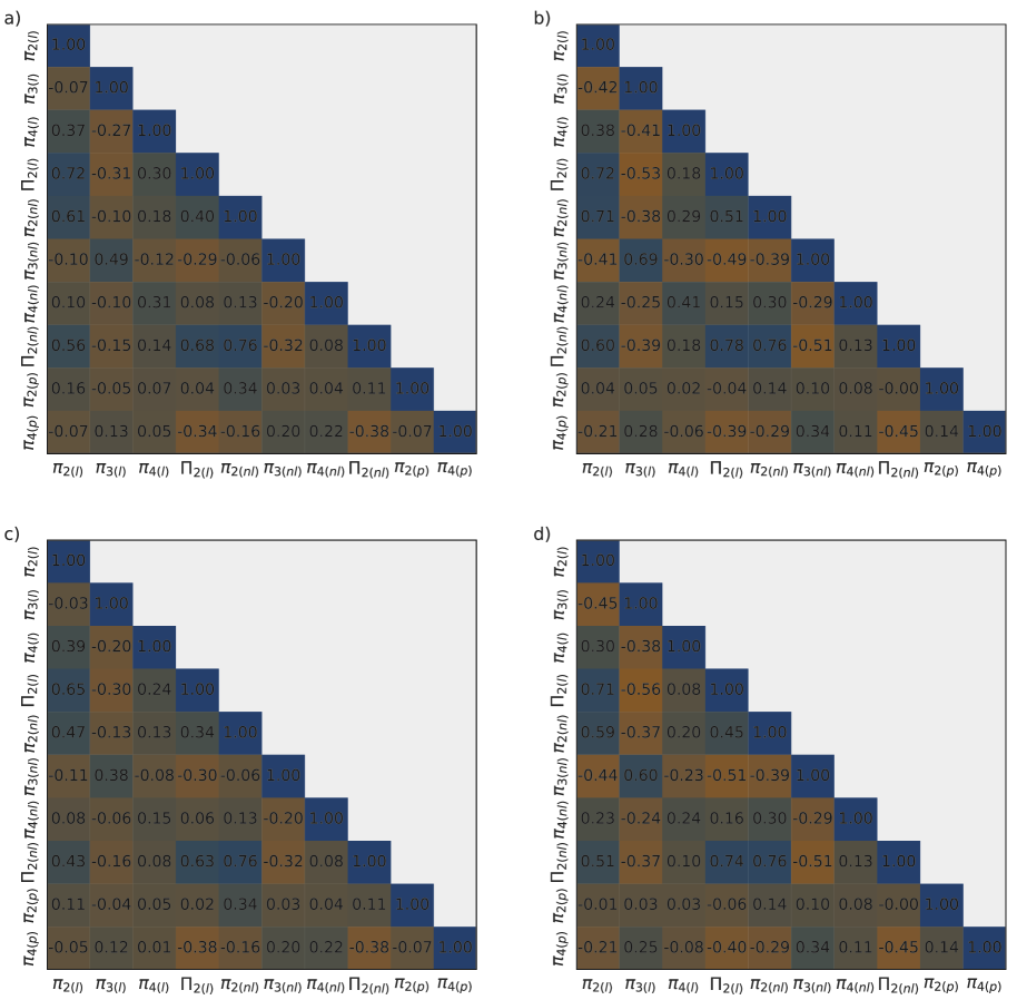
Figure 11: The correlation matrices of the indices for nonlocal flow paths originating at 0.2 sq. miles in the a) Chicago area and b) the northern New Jersey watersheds, and for nonlocal flow paths originating at 1 sq. mile in the c) Chicago area and d) northern New Jersey watersheds. All cases are based on the 100-year event, and the local flow paths originating at a contributing area of 0.01 sq. miles. The Chicago watersheds are HUCs 071200030101, 071200040403, 071200040505, and 071200040506, and the northern New Jersey watersheds are HUCs 020301030606, 020301030503, 020301030703, and 020301030804.

Appendix E Logistic regression algorithm

For flood extent prediction, We use the logistic regression model, a subset of the Generalized Linear Models (GLM) class. GLMs allow the response variable (i.e., the prediction), in this case probability of flooding, to have arbitrary distributions, and an arbitrary function of the response variable, called the link function, to vary linearly with the features or predictors. GLMs consist of three elements (Nelder and Wedderburn, 1972): 1) An exponential family of probability distributions e.g., Gaussian, Poisson, 2) A linear predictor $\eta=\vec{X}\vec{\beta}$, which is a linear combination of unknown parameters (i.e., weights), $\vec{\beta}$, with the feature vector (of dimensionless indices), $\vec{X}$, and 3) A link function, $g(\eta)$, such that $E(y|\vec{X})=\mu=g^{-1}(\eta)$, where $E(y|\vec{X})$ refers to the expectation of the response variable $y$ conditional on the feature vector, $\vec{X}$.

For the logistic regression, the link function is both the logit function and is the logistic distribution quantile function, i.e.,

$$g(\mu)=\text{ln}\left(\frac{p}{1-p}\right)=\vec{X}\vec{\beta},$$ (38)

where for a binary response (represented by a Bernoulli distribution), the expectation, $E(y|\vec{X})=\mu$, is equal to the probability, $p$, of an outcome of 1, i.e., $\mu=p$.

Accordingly, by inverting link function of Eq. (38), we retrieve the logistic function, i.e.,

$$p(\vec{X})=\frac{1}{1+e^{-\vec{X}\vec{\beta}}},$$ (39)

which provides the probability of an outcome based on the parameter weights $\vec{\beta}$ and features vector $\vec{X}$. Thus, for the dimensionless indices (i.e., features) of a given point, $\vec{X}_{m}$ (in a series indexed by $m$), the probability of an outcome of 1 is $p_{m}=p(\vec{X}_{m})$ where $p(\cdot)$ is given by Eq. (39). The probability of the outcome from $p(\vec{X}_{m})$ then is tuned (by adjusting the parameters $\vec{\beta}$) such that it aligns with the probability of flooded and not flooded observations, as described by a Bernoulli distribution i.e., $F(k;p)=p_{k}^{k}(1-p_{k})^{1-k}$ for $k\in\{0,1\}$, where $k=1$ and $k=0$, for flooded and non-flooded points, respectively.

The ML training, tunes the unknown parameters, $\vec{\beta}$, such that the logistic regression prediction best matches a given set of observations. For a set of observations (i.e., ground truth data), $Y$, the best fit to the data is found by maximizing the likelihood function $\mathcal{L}(\vec{\beta}|Y)$, i.e.,

$$\mathcal{L}(\vec{\beta}|Y)=\prod_{Y_{m}=1}p_{m}\prod_{Y_{m}=0}(1-p_{m})$$ (40)

where $p_{m}=p(\vec{X}_{m})$ based on Eq. (39), $m$ is an index for each grid cell (or geographic point) over the watershed, $Y_{m}=1$ when an observation is flooded, $Y_{m}=0$ when an observation is not flooded, and $\mathcal{L}$ describes the joint probability of the ground truth data as a function of the parameters $\vec{\beta}$. The optimal set of parameters is found by setting $\hat{\vec{\beta}}=\text{argmax}_{\vec{\beta}}\mathcal{L}(\vec{\beta}|Y)$.

Appendix F F-score

Binary classification produces predictions of true positives (TP), true negatives (TN), false positives (FP), and false negatives (FN). A successful statistical inference model maximizes TP and TN relative to TP and TN. These four categories (i.e., TP, TN, FP, and FN) are preferred over raw accuracy for imbalanced datasets such as flood datasets where, in most cases, dry areas exceed flooded areas in extent. The raw accuracy is calculated as

$$\text{accuracy}=\frac{\text{TP}+\text{TN}}{\text{All data points}}=\frac{\text{TP}+\text{TN}}{\text{TP}+\text{TN}+\text{FP}+\text{FN}}.$$ (41)

Basing model performance on the raw accuracy of Equation 41 is inappropriate for imbalance data because it allows for models to perform poorly on the minority class. For example, if a geospatial dataset is 5% flooded by extent, one can train a model with 95% accuracy by predicting all pixels as dry.

The F-score is an improvement on raw accuracy for imbalanced data. Once the model is trained, it is evaluated by calculating the F-score on the test set, which weights recall as $\beta>0$ more significant than precision, i.e., (Murphy, 2022)

$$F_{\beta}=\frac{1}{\frac{1}{1+\beta^{2}}\frac{1}{P}+\frac{\beta^{2}}{1+\beta^{2}}\frac{1}{R}},$$ (42)

where $P$ is written as

$$P=\frac{\text{TP}}{\text{TP}+\text{FP}},$$ (43)

and $R$ is written as

$$R=\frac{\text{TP}}{\text{TP}+\text{FN}}.$$ (44)

When the precision and recall are equally weighted, i.e., $\beta=1$, then we retrieve the F₁-score that is the harmonic mean of the precision, $P$, and recall, $R$, i.e.,

$$F_{1}=\frac{2\,P\,R}{P+R}.$$ (45)

Equations 43 and 44 both have TP in their numerators and denominators which suggests that the F score prioritizes the positive class over the negative one. This is appropriate when the imbalance in the data is in the negative class’ favor; this is when the positive class is in the minority. More intuitively, the recall, $R$, also may be thought of as a ’hit rate’, i.e., the fraction of predictions that capture flooding accurately in comparison to the assumed ground truth data, while 1 minus the precision, $1-P$, may be though of as a ’false alarm rate’, i.e., the fraction of predictions that falsely predicted flooding in comparison to the assumed ground truth data.