Optimal Covariance Steering for Discrete-Time Linear Stochastic Systems

Abstract

In this paper, we study the optimal control problem for steering the state covariance of a discrete-time linear stochastic system over a finite time horizon. First, we establish the existence and uniqueness of the optimal control law for a quadratic cost function. Then, we show the separation of the optimal mean and the covariance steering problems. We also develop efficient computational methods for solving for the optimal control law, which is identified as the solution to a semi-definite program. The effectiveness of the proposed approach is demonstrated through numerical examples. In the process, we also obtain some novel theoretical results for a matrix Riccati difference equation, which may be of independent interest.

I Introduction

In recent years, the need to quantify and control the uncertainty in physical systems has prompted a burgeoning interest in studying the evolution of the distribution of the trajectories of stochastic systems. A special case of this point of view is covariance control, the earliest research of which can be traced back to a series of articles from 1985 onward on the assignability of the state covariance via state feedback over an infinite time horizon [1, 2, 3, 4, 5]. The optimal control that assigns a prescribed stationary state covariance with minimum control energy was developed in [6]. More recent studies address the problem of optimally steering the state covariance of a linear stochastic system over a finite time horizon [7, 8, 9, 10, 11]. For discrete-time optimal covariance steering, the approach taken by most state-of-the-art current work involves three steps: 1) reformulate the problem as an optimization problem in an augmented state space that includes the entire history of the state; 2) relax the non-convex constraints to convex constraints for a tractable convex optimization problem; 3) solve the convex optimization problem numerically to approximate the optimal control. One of the reasons for the above approach is that when chance constraints on the sample paths of the input and the state are imposed, the state-mean and state-covariance constraints are coupled, which makes it difficult to find the optimal control analytically [7, 8, 10]. When there are no chance constraints, the desired terminal covariance can be replaced with a soft constraint on the Wasserstein distance between the desired and the actual terminal Gaussian distributions, which can be solved using a randomized state feedback control in terms of a (convex) semi-definite programming (SDP) [12]. Finite-horizon covariance control has also been applied to a model-predictive-control setting [13, 14], in which at each time step an optimal covariance steering problem is solved in a receding-horizon fashion.

In addition to controlling the first two moments of the state of a stochastic system, it is also possible to steer the entire state distribution using optimization techniques [15]. The continuous-time counterpart for finite-horizon covariance steering is investigated in [16, 17, 18, 19, 20]. By quantifying the uncertainty directly, covariance control theory can be applied to various practical scenarios, such as spacecraft landing [21], spacecraft trajectory optimization [22], vehicle path planning [23, 14], and aircraft motion planning [24].

Despite the success in finding an approximate solution to the optimal covariance steering problem using convex optimization, little is known regarding fundamental questions, such as the existence and uniqueness of the optimal control. Additionally, very little is known regarding the conservativeness of the approximate solution compared to the optimal control, if one exists. In this paper, we provide answers to these questions for the discrete-time covariance steering case.

The contributions of this work can be summarized as follows: We first establish an analytic result on the existence and uniqueness of the optimal control law for steering the state covariance of a discrete-time linear stochastic system with respect to a quadratic cost function. Some interesting properties of a matrix Riccati difference equation are derived in the process. Then, in the absence of any constraints, we demonstrate that the optimal state mean and covariance can be controlled independently. Next, we show that the optimal control law can be computed via a problem reformulation as an SDP using a lossless convex relaxation. In other words, it is shown that the optimal solution to the SDP problem also solves the original non-convex covariance steering problem. Lastly, we compare the results from the SDP formulation and from the direct application of Newton’s method through a numerical example. To the best of our knowledge, this is the first work to analyze the existence and uniqueness of the optimal control for steering the state covariance to any given terminal value in discrete time and to show that the optimal control can be solved exactly.

The rest of the paper is organized as follows. The discrete-time covariance steering problem considered in this paper is formulated in Section II. The existence and uniqueness of the optimal control as well as the separation of the optimal mean and covariance steering problems are shown in Section III. The methods for computing the optimal control are provided in Section IV. A numerical example is presented in Section V. For conciseness and ease of exposition, most of the proofs and auxiliary results are given in the Appendices.

II Problem Formulation

Consider the linear time-varying stochastic system corrupted by noise,

$$x_{k+1}=A_{k}x_{k}+B_{k}u_{k}+D_{k}w_{k},\quad k=0,1,\dots,N-1,$$ (1)

where $x_{k}\in\mathbb{R}^{n}$ is the state, $u_{k}\in\mathbb{R}^{p}$ is the control input at time step $k$, $w_{k}\in\mathbb{R}^{q}$ is the square integrable noise independent of $x_{k}$ and $u_{k}$, such that $\mathbb{E}\left[w_{k}\right]=0$ and $\mathbb{E}\left[w_{k}w_{k}^{\mbox{\tiny\sf T}}\right]=I_{n}$, and $A_{k}\in\mathbb{R}^{n\times n}$, $B_{k}\in\mathbb{R}^{n\times p}$, and $D_{k}\in\mathbb{R}^{n\times q}$ are the coefficient matrices.

Assumption 1.

For all $k=0,1,\dots,N-1$, the matrix $A_{k}$ is invertible.

With Assumption 1, we can define the state transition matrix $\Phi_{A}(k,\ell)$ from time $\ell$ to $k$ as

$$\Phi_{A}(k,\ell)\triangleq\begin{cases}A_{k-1}A_{k-2}\cdots A_{\ell},&0\leq\ell<k\leq N,\\ I_{n},&0\leq\ell=k\leq N,\\ A_{k}^{-1}A_{k+1}^{-1}\cdots A_{\ell-1}^{-1},&0\leq k<\ell\leq N.\end{cases}$$

The reachability Gramian $G(k,\ell)$ of system (1) from time $\ell$ to $k$ is defined as

$$G(k,\ell)\triangleq\begin{cases}\sum_{i=\ell}^{k-1}\Phi_{A}(k,i+1)B_{i}B_{i}^{\mbox{\tiny\sf T}}\Phi_{A}(k,i+1)^{\mbox{\tiny\sf T}},&0\leq\ell<k\leq N,\\ 0_{n\times n},&0\leq\ell=k\leq N,\\ -\sum_{i=k}^{\ell-1}\Phi_{A}(k,i+1)B_{i}B_{i}^{\mbox{\tiny\sf T}}\Phi_{A}(k,i+1)^{\mbox{\tiny\sf T}},&0\leq k<\ell\leq N.\end{cases}$$

Assumption 2.

System (1) is controllable from time $0$ to $N$. That is, the reachability Gramian $G(N,0)\succ 0$.

The initial state $x_{0}$ and the desired terminal state $x_{N}$ are characterized by their mean and their covariance matrices given by

$$\mathbb{E}\left[x_{0}\right]=\bar{\mu}_{0},\quad \mathbb{E}\big{[}(x_{0}-\bar{\mu}_{0})(x_{0}-\bar{\mu}_{0})^{\mbox{\tiny\sf T}}\big{]}=\bar{\Sigma}_{0}\succ 0,$$ (2a)

$$\mathbb{E}\left[x_{N}\right]=\bar{\mu}_{N},\quad \mathbb{E}\big{[}(x_{N}-\bar{\mu}_{N})(x_{N}-\bar{\mu}_{N})^{\mbox{\tiny\sf T}}\big{]}=\bar{\Sigma}_{N}\succ D_{N-1}D_{N-1}^{\mbox{\tiny\sf T}}.$$ (2b)

A control input $\{u_{k}\}_{k=0}^{N-1}$, is said to be admissible if each $u_{k}$ depends only on $k$ and, perhaps, on the past history of the states $x_{0}$, $x_{1}$, $\dots$, $x_{k}$, such that the desired boundary constraints (2) are satisfied. Without loss of generality, we may assume that the desired terminal state mean is $\bar{\mu}_{N}=0$. In this case, we introduce a cost functional defined by

$$J\triangleq\mathbb{E}\left[\sum_{k=0}^{N-1}x_{k}^{\mbox{\tiny\sf T}}Q_{k}x_{k}+u_{k}^{\mbox{\tiny\sf T}}R_{k}u_{k}\right],$$ (3)

where $Q_{k}\succeq 0$ and $R_{k}\succ 0$ are matrices of dimensions $n\times n$ and $p\times p$, respectively. The problem is to determine the optimal admissible control $u_{k}^{*}$ that minimizes the quadratic cost (3) subject to the initial and terminal state constraints (2).

III Existence and Uniqueness of the Optimal Control

The main theorem on the existence and uniqueness of the optimal control is summarized below.

Theorem 1.

Let $\bar{\Sigma}_{0}\succ 0$ and $\bar{\Sigma}_{N}\succ D_{N-1}D_{N-1}^{\mbox{\tiny\sf T}}$. Under Assumptions 1 and 2, the unique optimal control law that solves the covariance steering problem for system (1) is given, for all $k=0,1,\dots,N-1$, by

$$u^{*}_{k} =-\big{(}R_{k}+B_{k}^{\mbox{\tiny\sf T}}\Pi_{k+1}B_{k}\big{)}^{-1}B_{k}^{\mbox{\tiny\sf T}}\Pi_{k+1}A_{k}x_{k}-\big{(}R_{k}+B_{k}^{\mbox{\tiny\sf T}}\Pi_{k+1}B_{k}\big{)}^{-1}B_{k}^{\mbox{\tiny\sf T}}\Phi_{\bar{A}}(N,k+1)^{\mbox{\tiny\sf T}}$$ (4)

$$\hskip 28.45274pt\times\left(\sum_{i=0}^{N-1}\Phi_{\bar{A}}(N,i+1)B_{i}\big{(}R_{i}+B_{i}^{\mbox{\tiny\sf T}}\Pi_{i+1}B_{i}\big{)}^{-1}B_{i}^{\mbox{\tiny\sf T}}\Phi_{\bar{A}}(N,i+1)^{\mbox{\tiny\sf T}}\right)^{-1}\Big{(}\Phi_{\bar{A}}(N,0)\bar{\mu}_{0}-\bar{\mu}_{N}\Big{)},$$

where $\Pi_{k}$ is the unique solution of the coupled matrix difference equations

$$\Pi_{k}=A_{k}^{\mbox{\tiny\sf T}}\Pi_{k+1}\big{(}I_{n}+B_{k}R_{k}^{-1}B_{k}^{\mbox{\tiny\sf T}}\Pi_{k+1}\big{)}^{-1}A_{k}+Q_{k},$$ (5a)

$$\Sigma_{k+1}=\big{(}I_{n}+B_{k}R_{k}^{-1}B_{k}^{\mbox{\tiny\sf T}}\Pi_{k+1}\big{)}^{-1}A_{k}\Sigma_{k}A_{k}^{\mbox{\tiny\sf T}}\big{(}I_{n}+\Pi_{k+1}B_{k}R_{k}^{-1}B_{k}^{\mbox{\tiny\sf T}}\big{)}^{-1}+D_{k}D_{k}^{\mbox{\tiny\sf T}},$$ (5b)

$$\Sigma_{0}=\bar{\Sigma}_{0},\quad\Sigma_{N}=\bar{\Sigma}_{N},$$ (5c)

and, for all $k=0,1,\dots,N-1$, satisfies $R_{k}+B_{k}^{\mbox{\tiny\sf T}}\Pi_{k+1}B_{k}\succ 0$, and where $\Phi_{\bar{A}}(\ell,s)$ is the state transition matrix of

$$\bar{A}_{k}\triangleq\big{(}I_{n}+B_{k}R_{k}^{-1}B_{k}^{\mbox{\tiny\sf T}}\Pi_{k+1}\big{)}^{-1}A_{k},\quad k=0,1,\dots,N-1,$$ (6)

from time $s$ to $\ell$, which is defined by

$$\Phi_{\bar{A}}(\ell,s)\triangleq\begin{cases}\bar{A}_{\ell-1}\bar{A}_{\ell-2}\cdots\bar{A}_{s},&0\leq s<\ell\leq N,\\ I_{n},&0\leq s=\ell\leq N,\\ \bar{A}_{\ell}^{-1}\bar{A}_{\ell+1}^{-1}\cdots\bar{A}_{s-1}^{-1},&0\leq\ell<s\leq N.\end{cases}$$ (7)

The corresponding optimal process is given by

$$x_{k+1}^{*} =\big{(}I_{n}+B_{k}R_{k}^{-1}B_{k}^{\mbox{\tiny\sf T}}\Pi_{k+1}\big{)}^{-1}A_{k}x_{k}^{*}-B_{k}\big{(}R_{k}+B_{k}^{\mbox{\tiny\sf T}}\Pi_{k+1}B_{k}\big{)}^{-1}B_{k}^{\mbox{\tiny\sf T}}\Phi_{\bar{A}}(N,k+1)^{\mbox{\tiny\sf T}}$$

$$\hskip 28.45274pt\times\left(\sum_{i=0}^{N-1}\Phi_{\bar{A}}(N,i+1)B_{i}\big{(}R_{i}+B_{i}^{\mbox{\tiny\sf T}}\Pi_{i+1}B_{i}\big{)}^{-1}B_{i}^{\mbox{\tiny\sf T}}\Phi_{\bar{A}}(N,i+1)^{\mbox{\tiny\sf T}}\right)^{-1}\Big{(}\Phi_{\bar{A}}(N,0)\bar{\mu}_{0}-\bar{\mu}_{N}\Big{)}$$

$$\hskip 227.62204pt+D_{k}w_{k},\qquad k=0,1,\dots,N-1.$$ (8)

Property 1.

For all $k=0,1,\dots,N-1$, the matrix $R_{k}+B_{k}^{\mbox{\tiny\sf T}}\Pi_{k+1}B_{k}\succ 0$.

At this point, it suffices to note that Property 1 does not follow immediately from $R_{k}\succ 0$, since $\Pi_{k+1}$ is not necessarily positive semi-definite. Necessary and sufficient conditions for Property 1 to hold are provided by Theorem 2 in Section III-B.

Remark 1.

Since $R_{k}\succ 0$, Property 1 implies that, for all $k=0,1,\dots,N-1$, the matrix $I_{n}+B_{k}R_{k}^{-1}B_{k}^{\mbox{\tiny\sf T}}\Pi_{k+1}$ is invertible according to the Sherman–Morrison–Woodbury formula [25].

Remark 2.

In light of (5b), it is clear that, under Assumption 1 and Property 1, if $\Sigma_{0}\succ 0$, then, for all $k=0,1,\dots,N-1$, $\Sigma_{k+1}\succ D_{k}D_{k}^{\mbox{\tiny\sf T}}$.

Remark 3.

In the continuous-time case, when $D(t)D(t)^{\mbox{\tiny\sf T}}\equiv\kappa B(t)R^{-1}(t)B(t)^{\mbox{\tiny\sf T}}$ for some $\kappa>0$, there exists a closed-form solution of $\Pi(0)$ for the continuous-time counterpart of the coupled matrix equations (5) [16, 18]. In the discrete-time case, however, there may not be a closed-form solution for $\Pi_{0}$ even when $D_{k}D_{k}^{\mbox{\tiny\sf T}}\equiv B_{k}R_{k}^{-1}B_{k}^{\mbox{\tiny\sf T}}$. Interestingly, a closed-form solution exists for the discrete-time maximum entropy optimal density control problem [26].

The rest of this section is dedicated to proving Theorem 1 and the separation of mean and covariance steering problems, for which several intermediate results are needed. First, we show that (4) is a candidate optimal control law, provided the coupled matrix difference equations (5) admit a solution that satisfies Property 1. Then, we give a necessary and sufficient condition for the Riccati difference equation (5a) to have a unique solution. Next, we present necessary and sufficient conditions for the solution of (5a) to satisfy Property 1. After that, we show the existence and uniqueness of the solution to the coupled equations (5), which completes the proof of Theorem 1. Finally, we show the separation of mean and covariance steering.

III-A Candidate Optimal Control

A candidate optimal control law is derived using a “completion of squares” argument. To this end, let $\Pi_{0}$, $\Pi_{1}$, $\dots$, $\Pi_{N}\in\mathbb{R}^{n\times n}$ be symmetric matrices, and let $\psi_{0}$, $\psi_{1}$, $\dots$, $\psi_{N}\in\mathbb{R}^{n}$. In view of (2), the expected values $\mathbb{E}\big{[}x_{0}^{\mbox{\tiny\sf T}}\Pi_{0}x_{0}\big{]}$, $\mathbb{E}\big{[}x_{N}^{\mbox{\tiny\sf T}}\Pi_{N}x_{N}\big{]}$, $\mathbb{E}\big{[}\psi_{0}^{\mbox{\tiny\sf T}}x_{0}\big{]}$, and $\mathbb{E}\big{[}\psi_{N}^{\mbox{\tiny\sf T}}x_{N}\big{]}$ are independent of the control. Then, the cost function (3) can be equivalently written as

$$J =\mathbb{E}\left[\sum_{k=0}^{N-1}x_{k}^{\mbox{\tiny\sf T}}Q_{k}x_{k}+u_{k}^{\mbox{\tiny\sf T}}R_{k}u_{k}\right]+\mathbb{E}\big{[}x_{N}^{\mbox{\tiny\sf T}}\Pi_{N}x_{N}-x_{0}^{\mbox{\tiny\sf T}}\Pi_{0}x_{0}+2\psi_{N}^{\mbox{\tiny\sf T}}x_{N}-2\psi_{0}^{\mbox{\tiny\sf T}}x_{0}\big{]}$$

$$=\mathbb{E}\left[\sum_{k=0}^{N-1}x_{k}^{\mbox{\tiny\sf T}}Q_{k}x_{k}+u_{k}^{\mbox{\tiny\sf T}}R_{k}u_{k}+x_{k+1}^{\mbox{\tiny\sf T}}\Pi_{k+1}x_{k+1}-x_{k}^{\mbox{\tiny\sf T}}\Pi_{k}x_{k}+2\psi_{k+1}^{\mbox{\tiny\sf T}}x_{k+1}-2\psi_{k}^{\mbox{\tiny\sf T}}x_{k}\right]$$

$$=\mathbb{E}\Bigg{[}\sum_{k=0}^{N-1}x_{k}^{\mbox{\tiny\sf T}}Q_{k}x_{k}+u_{k}^{\mbox{\tiny\sf T}}R_{k}u_{k}+\big{(}x_{k}^{\mbox{\tiny\sf T}}A_{k}^{\mbox{\tiny\sf T}}+u_{k}^{\mbox{\tiny\sf T}}B_{k}^{\mbox{\tiny\sf T}}\big{)}\Pi_{k+1}\big{(}A_{k}x_{k}+B_{k}u_{k}\big{)}$$

$$\hskip 128.0374pt+w_{k}^{\mbox{\tiny\sf T}}D_{k}^{\mbox{\tiny\sf T}}\Pi_{k+1}D_{k}w_{k}-x_{k}^{\mbox{\tiny\sf T}}\Pi_{k}x_{k}+2\psi_{k+1}^{\mbox{\tiny\sf T}}\big{(}A_{k}x_{k}+B_{k}u_{k}\big{)}-2\psi_{k}^{\mbox{\tiny\sf T}}x_{k}\Bigg{]}$$

$$=\mathbb{E}\left[\sum_{k=0}^{N-1}x_{k}^{\mbox{\tiny\sf T}}\big{(}Q_{k}+A_{k}^{\mbox{\tiny\sf T}}\Pi_{k+1}A_{k}-\Pi_{k}\big{)}x_{k}+u_{k}^{\mbox{\tiny\sf T}}\big{(}R_{k}+B_{k}^{\mbox{\tiny\sf T}}\Pi_{k+1}B_{k}\big{)}u_{k}\right]\!+\sum_{k=0}^{N-1}\operatorname{trace}\big{(}\Pi_{k+1}D_{k}D_{k}^{\mbox{\tiny\sf T}}\big{)}$$

$$\hskip 42.67912pt+\mathbb{E}\left[\sum_{k=0}^{N-1}x_{k}^{\mbox{\tiny\sf T}}A_{k}^{\mbox{\tiny\sf T}}\Pi_{k+1}B_{k}u_{k}+u_{k}^{\mbox{\tiny\sf T}}B_{k}^{\mbox{\tiny\sf T}}\Pi_{k+1}A_{k}x_{k}+2\psi_{k+1}^{\mbox{\tiny\sf T}}A_{k}x_{k}+2\psi_{k+1}^{\mbox{\tiny\sf T}}B_{k}u_{k}-2\psi_{k}^{\mbox{\tiny\sf T}}x_{k}\right].$$

Define the matrix $S_{k}\triangleq R_{k}+B_{k}^{\mbox{\tiny\sf T}}\Pi_{k+1}B_{k}$. Then, we have

$$J =\mathbb{E}\left[\sum_{k=0}^{N-1}\big{(}u_{k}^{\mbox{\tiny\sf T}}+x_{k}^{\mbox{\tiny\sf T}}A_{k}^{\mbox{\tiny\sf T}}\Pi_{k+1}B_{k}S_{k}^{-1}+\psi_{k+1}^{\mbox{\tiny\sf T}}B_{k}S_{k}^{-1}\big{)}S_{k}\big{(}u_{k}+S_{k}^{-1}B_{k}^{\mbox{\tiny\sf T}}\Pi_{k+1}A_{k}x_{k}+S_{k}^{-1}B_{k}^{\mbox{\tiny\sf T}}\psi_{k+1}\big{)}\right]$$

$$\hskip 56.9055pt+\mathbb{E}\left[\sum_{k=0}^{N-1}x_{k}^{\mbox{\tiny\sf T}}\big{(}Q_{k}+A_{k}^{\mbox{\tiny\sf T}}\Pi_{k+1}A_{k}-\Pi_{k}-A_{k}^{\mbox{\tiny\sf T}}\Pi_{k+1}B_{k}S_{k}^{-1}B_{k}^{\mbox{\tiny\sf T}}\Pi_{k+1}A_{k}\big{)}x_{k}\right]$$

$$\hskip 56.9055pt+\mathbb{E}\left[\sum_{k=0}^{N-1}2\Big{(}\psi_{k+1}^{\mbox{\tiny\sf T}}\big{(}I_{n}+B_{k}R_{k}^{-1}B_{k}^{\mbox{\tiny\sf T}}\Pi_{k+1}\big{)}^{-1}A_{k}-\psi_{k}^{\mbox{\tiny\sf T}}\Big{)}x_{k}\right]$$

$$\hskip 56.9055pt+\sum_{k=0}^{N-1}\Big{[}\operatorname{trace}\big{(}\Pi_{k+1}D_{k}D_{k}^{\mbox{\tiny\sf T}}\big{)}-\psi_{k+1}^{\mbox{\tiny\sf T}}B_{k}S_{k}^{-1}B_{k}^{\mbox{\tiny\sf T}}\psi_{k+1}\Big{]}.$$

To this end, let $\Pi_{k}$ satisfy the difference equation (5a) and let $\psi_{k}$ satisfy the difference equation

$$\psi_{k}=A_{k}^{\mbox{\tiny\sf T}}\big{(}I_{n}+\Pi_{k+1}B_{k}R_{k}^{-1}B_{k}^{\mbox{\tiny\sf T}}\big{)}^{-1}\psi_{k+1}.$$ (9)

Then, we obtain

$$J =\mathbb{E}\left[\sum_{k=0}^{N-1}\big{(}u_{k}^{\mbox{\tiny\sf T}}+x_{k}^{\mbox{\tiny\sf T}}A_{k}^{\mbox{\tiny\sf T}}\Pi_{k+1}B_{k}S_{k}^{-1}+\psi_{k+1}^{\mbox{\tiny\sf T}}B_{k}S_{k}^{-1}\big{)}S_{k}\big{(}u_{k}+S_{k}^{-1}B_{k}^{\mbox{\tiny\sf T}}\Pi_{k+1}A_{k}x_{k}+S_{k}^{-1}B_{k}^{\mbox{\tiny\sf T}}\psi_{k+1}\big{)}\right]$$

$$\hskip 199.16928pt+\sum_{k=0}^{N-1}\Big{[}\operatorname{trace}\big{(}\Pi_{k+1}D_{k}D_{k}^{\mbox{\tiny\sf T}}\big{)}-\psi_{k+1}^{\mbox{\tiny\sf T}}B_{k}S_{k}^{-1}B_{k}^{\mbox{\tiny\sf T}}\psi_{k+1}\Big{]}.$$

Since $\sum_{k=0}^{N-1}\big{[}\operatorname{trace}\big{(}\Pi_{k+1}D_{k}D_{k}^{\mbox{\tiny\sf T}}\big{)}-\psi_{k+1}^{\mbox{\tiny\sf T}}B_{k}S_{k}^{-1}B_{k}^{\mbox{\tiny\sf T}}\psi_{k+1}\big{]}$ is independent of the control, a candidate optimal control is given by

$$u^{*}_{k}=-\big{(}R_{k}+B_{k}^{\mbox{\tiny\sf T}}\Pi_{k+1}B_{k}\big{)}^{-1}B_{k}^{\mbox{\tiny\sf T}}\Pi_{k+1}A_{k}x_{k}-\big{(}R_{k}+B_{k}^{\mbox{\tiny\sf T}}\Pi_{k+1}B_{k}\big{)}^{-1}B_{k}^{\mbox{\tiny\sf T}}\psi_{k+1},\quad k=0,1,\dots,N-1,$$ (10)

provided that $S_{k}\succ 0$, that is, Property 1 holds.

Hence, for all $k=0,1,\dots,N-1$, the corresponding optimal process is given by

$$x_{k+1}^{*}=\big{(}I_{n}+B_{k}R_{k}^{-1}B_{k}^{\mbox{\tiny\sf T}}\Pi_{k+1}\big{)}^{-1}A_{k}x_{k}^{*}-B_{k}\big{(}R_{k}+B_{k}^{\mbox{\tiny\sf T}}\Pi_{k+1}B_{k}\big{)}^{-1}B_{k}^{\mbox{\tiny\sf T}}\psi_{k+1}+D_{k}w_{k}.$$ (11)

Let $\mu_{k}\triangleq\mathbb{E}[x_{k}^{*}]$ be the state mean at time $k=0,1,\dots,N$, which satisfies the difference equation

$$\mu_{k+1}=\big{(}I_{n}+B_{k}R_{k}^{-1}B_{k}^{\mbox{\tiny\sf T}}\Pi_{k+1}\big{)}^{-1}A_{k}\mu_{k}-B_{k}\big{(}R_{k}+B_{k}^{\mbox{\tiny\sf T}}\Pi_{k+1}B_{k}\big{)}^{-1}B_{k}^{\mbox{\tiny\sf T}}\psi_{k+1}$$ (12)

with boundary conditions $\mu_{0}=\bar{\mu}_{0}$ and $\mu_{N}=\bar{\mu}_{N}$.

In light of (9) and (6), we can rewrite equation (12) as

$$\mu_{k+1}=\bar{A}_{k}\mu_{k}-B_{k}\big{(}R_{k}+B_{k}^{\mbox{\tiny\sf T}}\Pi_{k+1}B_{k}\big{)}^{-1}B_{k}^{\mbox{\tiny\sf T}}\Phi_{\bar{A}}(N,k+1)^{\mbox{\tiny\sf T}}\psi_{N}.$$

From the above equation and the boundary conditions $\mu_{0}=\bar{\mu}_{0}$ and $\mu_{N}=\bar{\mu}_{N}$, we obtain

$$\bar{\mu}_{N}=\Phi_{\bar{A}}(N,0)\bar{\mu}_{0}-\sum_{i=0}^{N-1}\Phi_{\bar{A}}(N,i+1)B_{i}\big{(}R_{i}+B_{i}^{\mbox{\tiny\sf T}}\Pi_{i+1}B_{i}\big{)}^{-1}B_{i}^{\mbox{\tiny\sf T}}\Phi_{\bar{A}}(N,i+1)^{\mbox{\tiny\sf T}}\psi_{N}.$$ (13)

To proceed, we make use of the fact that

$$\sum_{i=0}^{N-1}\Phi_{\bar{A}}(N,i+1)B_{i}\big{(}R_{i}+B_{i}^{\mbox{\tiny\sf T}}\Pi_{i+1}B_{i}\big{)}^{-1}B_{i}^{\mbox{\tiny\sf T}}\Phi_{\bar{A}}(N,i+1)^{\mbox{\tiny\sf T}}\succ 0,$$ (14)

which is proven as Lemma 2 in Appendix A. From equations (13) and (14) we obtain

$$\psi_{N}=\left(\sum_{i=0}^{N-1}\Phi_{\bar{A}}(N,i+1)B_{i}\big{(}R_{i}+B_{i}^{\mbox{\tiny\sf T}}\Pi_{i+1}B_{i}\big{)}^{-1}B_{i}^{\mbox{\tiny\sf T}}\Phi_{\bar{A}}(N,i+1)^{\mbox{\tiny\sf T}}\right)^{-1}\Big{(}\Phi_{\bar{A}}(N,0)\bar{\mu}_{0}-\bar{\mu}_{N}\Big{)}.$$

It then follows from (9) and the above equation that

$$\psi_{k+1}=$$

$$\Phi_{\bar{A}}(N,k+1)^{\mbox{\tiny\sf T}}\left(\sum_{i=0}^{N-1}\Phi_{\bar{A}}(N,i+1)B_{i}\big{(}R_{i}+B_{i}^{\mbox{\tiny\sf T}}\Pi_{i+1}B_{i}\big{)}^{-1}B_{i}^{\mbox{\tiny\sf T}}\Phi_{\bar{A}}(N,i+1)^{\mbox{\tiny\sf T}}\right)^{-1}\Big{(}\Phi_{\bar{A}}(N,0)\bar{\mu}_{0}-\bar{\mu}_{N}\Big{)}.$$ (15)

Plugging (III-A) into (10) and (11) yields (4) and (1), respectively.

It is clear from (11) and (12) that

$$x_{k+1}^{*}-\mu_{k+1}=\big{(}I_{n}+B_{k}R_{k}^{-1}B_{k}^{\mbox{\tiny\sf T}}\Pi_{k+1}\big{)}^{-1}A_{k}(x_{k}^{*}-\mu_{k})+D_{k}w_{k}.$$

Therefore, the state covariance $\Sigma_{k}\triangleq\mathbb{E}\big{[}(x_{k}^{*}-\mu_{k})(x_{k}^{*}-\mu_{k})^{\mbox{\tiny\sf T}}\big{]}$ at time $k=0,1,\dots,N$ satisfies the difference equation (5b) and the boundary conditions (5c).

We have thus shown the following result.

Proposition 1.

Assume there exist $\Pi_{k},\Sigma_{k}\in\mathbb{R}^{n\times n}$ such that, for $k=0,1,\dots,N-1$, Property 1 and the coupled equations (5) hold. Then, the state feedback control $u^{*}$ given by (4) is optimal for the covariance steering problem. Furthermore, if there exists a unique solution to the coupled equations (5), then, the optimal control $u^{*}$ is unique. The corresponding optimal process is given by (1).

Since $R_{k}\succ 0$ can always be absorbed into $B_{k}$ by defining $\hat{B}_{k}\triangleq B_{k}R_{k}^{-\frac{1}{2}}$, without loss of generality and for the sake of notational simplicity, for the rest of the proof of Theorem 1 we assume $R_{k}\equiv I_{p}$.

III-B Riccati Difference Equation

In this section, we give a necessary and sufficient condition for the unique solution $\Pi_{k}$ of the Riccati difference equation (5a) to exist from time $0$ to $N$. A stronger condition for the solution of (5a) to also satisfy Property 1 is provided as well.

To this end, let

$$M_{k}\triangleq\begin{bmatrix}A_{k}+B_{k}B_{k}^{\mbox{\tiny\sf T}}A_{k}^{-\mbox{\tiny\sf T}}Q_{k}&-B_{k}B_{k}^{\mbox{\tiny\sf T}}A_{k}^{-\mbox{\tiny\sf T}}\\ -A_{k}^{-\mbox{\tiny\sf T}}Q_{k}&A_{k}^{-\mbox{\tiny\sf T}}\end{bmatrix}\triangleq\begin{bmatrix}M_{k,1}&M_{k,2}\\ M_{k,3}&M_{k,4}\end{bmatrix},\quad k=0,1,\dots,N-1.$$ (16)

It can be checked that $M_{k}$ is invertible, as $A_{k}^{-\mbox{\tiny\sf T}}$ and its Schur complement $A_{k}+B_{k}B_{k}^{\mbox{\tiny\sf T}}A_{k}^{-\mbox{\tiny\sf T}}Q_{k}-B_{k}B_{k}^{\mbox{\tiny\sf T}}A_{k}^{-\mbox{\tiny\sf T}}A_{k}^{\mbox{\tiny\sf T}}A_{k}^{-\mbox{\tiny\sf T}}Q_{k}=A_{k}$ in $M_{k}$ are invertible. The state transition matrix of $M_{k}$ from time $s$ to $k$ is denoted by

$$\Phi_{M}(k,s)\triangleq\begin{bmatrix}\Phi_{11}(k,s)&\Phi_{12}(k,s)\\ \Phi_{21}(k,s)&\Phi_{22}(k,s)\end{bmatrix}\triangleq\begin{cases}M_{k-1}M_{k-2}\cdots M_{s},&0\leq s<k\leq N,\\ I_{2n},&0\leq s=k\leq N,\\ M_{k}^{-1}M_{k+1}^{-1}\cdots M_{s-1}^{-1},&0\leq k<s\leq N.\end{cases}$$ (17)

First, we give the condition for the existence of a solution to the matrix equation (5a).

Proposition 2.

Suppose Assumption 1 holds. Given an initial condition $\Pi_{0}$, (5a) has a solution from time $0$ to $N$ if and only if, for all $k=0,1,\dots,N$, the matrix $\Phi_{11}(k,0)+\Phi_{12}(k,0)\Pi_{0}$ is invertible. In this case, the unique solution of (5a) is given by

$$\Pi_{k}=\!\Big{(}\Phi_{21}(k,0)+\Phi_{22}(k,0)\Pi_{0}\Big{)}\!\Big{(}\Phi_{11}(k,0)+\Phi_{12}(k,0)\Pi_{0}\Big{)}^{-1}.$$ (18)

Proof.

The proof of Proposition 2 is given in Appendix B.  

Corollary 1.

Under Assumption 1, suppose the condition in Proposition 2 holds so that (5a) admits a solution $\Pi_{k}$ from time $0$ to $N$. Then, for all $\ell=0,1,\dots,N$,

$$\Pi_{k}=\!\Big{(}\Phi_{21}(k,\ell)+\Phi_{22}(k,\ell)\Pi_{\ell}\Big{)}\!\Big{(}\Phi_{11}(k,\ell)+\Phi_{12}(k,\ell)\Pi_{\ell}\Big{)}^{-1}.$$ (19)

Proof.

The proof of Corollary 1 is given in Appendix B.  

A number of necessary and sufficient conditions for the solution of the matrix Riccati difference equation (5a) to exist and to satisfy Property 1 are summarized below.

For the sake of notational simplicity, define, for all $k=0,1,\dots,N-1$, the matrices $L_{k}\triangleq\Phi_{11}(k,0)^{-1}A_{k}^{-1}B_{k}$, $T_{k}\triangleq I_{p}+B_{k}^{\mbox{\tiny\sf T}}A_{k}^{-\mbox{\tiny\sf T}}\big{(}Q_{k}-\Phi_{21}(k,0)\Phi_{11}(k,0)^{-1}\big{)}A_{k}^{-1}B_{k}\succ 0$, and

$$U_{k} \triangleq\begin{bmatrix}T_{k}&0&0&0\\ 0&T_{k-1}&0&0\\ 0&0&\ddots&0\\ 0&0&0&T_{0}\end{bmatrix}-\begin{bmatrix}L_{k}^{\mbox{\tiny\sf T}}\\ L_{k-1}^{\mbox{\tiny\sf T}}\\ \vdots\\ L_{0}^{\mbox{\tiny\sf T}}\end{bmatrix}\Pi_{0}\begin{bmatrix}L_{k}&L_{k-1}&\cdots&L_{0}\end{bmatrix}.$$

Theorem 2.

Under Assumption 1, the following statements are equivalent.

1. From time $0$ to $N$, the solution $\Pi_{k}$ of (5a) exists and satisfies Property 1 (respectively, exists).

2. For all $k=0,1,\dots,N-1$, $I_{p}+B_{k}^{\mbox{\tiny\sf T}}\Pi_{k+1}B_{k}\succ 0$ (respectively, is invertible).

3. For all $k=0,1,\dots,N-1$, $I_{p}-B_{k}^{\mbox{\tiny\sf T}}A_{k}^{-\mbox{\tiny\sf T}}\big{(}\Pi_{k}-Q_{k}\big{)}A_{k}^{-1}B_{k}\succ 0$ (respectively, is invertible).

4. For all $k=1,2,\dots,N-1$, $U_{0},U_{k}/U_{k-1}\succ 0$ (respectively, are invertible).

5. For all $k=0,1,\dots,N-1$, $U_{k}\succ 0$ (respectively, is invertible).

6. $U_{N-1}\succ 0$ (respectively, is invertible).

7. For all $k=0,1,\dots,N$, the eigenvalues of $I_{n}+\Phi_{11}(k,0)^{-1}\Phi_{12}(k,0)\Pi_{0}$ are positive (respectively, are nonzero).

8. All eigenvalues of $I_{n}+\Phi_{11}(N,0)^{-1}\Phi_{12}(N,0)\Pi_{0}$ are positive (respectively, are nonzero).

Under Assumptions 1 and 2, any of the above statements is also equivalent to the statement that

$$\Pi_{0}+\Phi_{12}(N,0)^{-1}\Phi_{11}(N,0)\prec 0~{}~{}\text{(respectively, is invertible)}.$$

Proof.

The proof of Theorem 2 is given in Appendix D.  

III-C Existence and Uniqueness of the Solution

In this section, we show that the solution of the coupled matrix difference equations (5) exists and it is unique. First, we need an alternative expression for the state transition matrix of $\bar{A}_{k}$ defined by (7) in Theorem 1.

Proposition 3.

Under Assumption 1, suppose the condition in Proposition 2 holds so that (5a) admits a solution $\Pi_{k}$ from time $0$ to $N$. For all $s,k=0,1,\dots,N$, the state transition matrix of $\bar{A}_{k}$ is given by

$$\Phi_{\bar{A}}(k,s)=\Phi_{11}(k,s)+\Phi_{12}(k,s)\Pi_{s}.$$ (20)

Proof.

The proof of Proposition 3 is given in Appendix E.  

The solution of the covariance equation (5b) is given as follows.

Proposition 4.

Under Assumptions 1 and 2, suppose $\Pi_{0}\prec-\Phi_{12}(N,0)^{-1}\Phi_{11}(N,0)$. Given $\Sigma_{0}=\bar{\Sigma}_{0}\succeq 0$, then, the solution $\Sigma_{k}$ of (5b) from time $0$ to $N$ is given by,

$$\Sigma_{k+1}=\Phi_{\bar{A}}(k+1,0)\bar{\Sigma}_{0}\Phi_{\bar{A}}(k+1,0)^{\mbox{\tiny\sf T}}+\sum_{i=0}^{k}\Phi_{\bar{A}}(k+1,i+1)D_{i}D_{i}^{\mbox{\tiny\sf T}}\Phi_{\bar{A}}(k+1,i+1)^{\mbox{\tiny\sf T}},$$ (21)

where $\Phi_{\bar{A}}(k,s)$ is given by (20) and $\Pi_{k}$ is given by (18). In particular,

$$\lim_{\Pi_{0}\to-\Phi_{12}(N,0)^{-1}\Phi_{11}(N,0)}\Sigma_{N}=D_{N-1}D_{N-1}^{\mbox{\tiny\sf T}}.$$

If $\bar{\Sigma}_{0}\succ 0$, then $\lim_{\Pi_{0}\to-\infty}\Sigma_{N}=+\infty$.

Proof.

Clearly, (21) is the solution of (5b). From Lemma 11 in Appendix D, as

$$\Pi_{0}\to-\Phi_{12}(N,0)^{-1}\Phi_{11}(N,0),$$

then $\Pi_{N}\to+\infty$. From (6), $\bar{A}_{N-1}\to 0_{n\times n}$. Thus, for all $i=0,1,\dots,N-1$, $\Phi_{\bar{A}}(N,i)\to 0_{n\times n}$. It follows that $\Sigma_{N}\to D_{N-1}D_{N-1}^{\mbox{\tiny\sf T}}$. On the other hand, since $\Phi_{12}(N,0)$ is invertible, and in view of (20), as $\Pi_{0}\to-\infty$, then it follows that $\Phi_{\bar{A}}(N,0)\to\infty$. When $\bar{\Sigma}_{0}\succ 0$, as $\Phi_{\bar{A}}(N,0)\to\infty$, then it follows that $\Sigma_{N}\to+\infty$.  

Proposition 4 can be used to provide an explicit map from $\Pi_{0}$ to $\Sigma_{N}$ for the coupled matrix difference equations (5a) and (5b) with $\Sigma_{0}=\bar{\Sigma}_{0}\succ 0$. Specifically, from (21) we can write

$$\Sigma_{N} =\Phi_{\bar{A}}(N,0)\bar{\Sigma}_{0}\Phi_{\bar{A}}(N,0)^{\mbox{\tiny\sf T}}+\sum_{i=0}^{N-1}\Phi_{\bar{A}}(N,i+1)D_{i}D_{i}^{\mbox{\tiny\sf T}}\Phi_{\bar{A}}(N,i+1)^{\mbox{\tiny\sf T}}$$

$$=\Phi_{\bar{A}}(N,0)\bigg{[}\bar{\Sigma}_{0}+\sum_{i=0}^{N-1}\Phi_{\bar{A}}(0,i+1)D_{i}D_{i}^{\mbox{\tiny\sf T}}\Phi_{\bar{A}}(0,i+1)^{\mbox{\tiny\sf T}}\bigg{]}\Phi_{\bar{A}}(N,0)^{\mbox{\tiny\sf T}}.$$ (22)

Define the sets $\mathcal{P}\triangleq\big{\{}\Pi\in\mathbb{R}^{n\times n}\,|\,\Pi=\Pi^{\mbox{\tiny\sf T}}\prec-\Phi_{12}(N,0)^{-1}\Phi_{11}(N,0)\big{\}}$ and $\mathcal{R}\triangleq\big{\{}\Sigma\in\mathbb{R}^{n\times n}\,|\,\Sigma=\Sigma^{\mbox{\tiny\sf T}}\succ D_{N-1}D_{N-1}^{\mbox{\tiny\sf T}}\big{\}}$. In light of (III-C) and (20), let $f:\mathcal{P}\to\mathcal{R}$ be defined by $\Sigma_{N}=f(\Pi_{0})$, where

$$f(\Pi_{0})=\Big{(}\Phi_{11}(N,0)+\Phi_{12}(N,0)\Pi_{0}\Big{)}\bigg{[}\bar{\Sigma}_{0}+\sum_{i=0}^{N-1}\Big{(}\Phi_{11}(i+1,0)+\Phi_{12}(i+1,0)\Pi_{0}\Big{)}^{-1}D_{i}D_{i}^{\mbox{\tiny\sf T}}\\ \times\Big{(}\Phi_{11}(i+1,0)^{\mbox{\tiny\sf T}}+\Pi_{0}\Phi_{12}(i+1,0)^{\mbox{\tiny\sf T}}\Big{)}^{-1}\bigg{]}\Big{(}\Phi_{11}(N,0)^{\mbox{\tiny\sf T}}+\Pi_{0}\Phi_{12}(N,0)^{\mbox{\tiny\sf T}}\Big{)}.$$ (23)

Similarly to [20], when $n>1$, the map $f$ may not be monotone in the Loewner order; however, when $n=1$, $f$ is monotonically decreasing.

To this end, let us compute the Jacobian of the map $f$ defined by (23). For notational simplicity, we will use the notation $\Phi_{ij}^{k,0}\triangleq\Phi_{ij}(k,0)$, where $i,j\in\{1,2\}$ and let $\Delta\Pi_{0}$ denote a small increment in $\Pi_{0}$. Then, from [27] we can write

$$\Big{(}\Phi_{11}^{i+1,0}+\Phi_{12}^{i+1,0}\Pi_{0}+\Phi_{12}^{i+1,0}\Delta\Pi_{0}\Big{)}^{-1}=\Big{(}\Phi_{11}^{i+1,0}+\Phi_{12}^{i+1,0}\Pi_{0}\Big{)}^{-1}\\ -\Big{(}\Phi_{11}^{i+1,0}+\Phi_{12}^{i+1,0}\Pi_{0}\Big{)}^{-1}\Phi_{12}^{i+1,0}\Delta\Pi_{0}\Big{(}\Phi_{11}^{i+1,0}+\Phi_{12}^{i+1,0}\Pi_{0}\Big{)}^{-1}+O\Big{(}\big{\|}\Delta\Pi_{0}\big{\|}^{2}\Big{)}.$$

After collecting all the first order terms of $\Delta\Pi_{0}$, we obtain

$$f\big{(}\Pi_{0}+\Delta\Pi_{0}\big{)}-f\big{(}\Pi_{0}\big{)}=O\Big{(}\big{\|}\Delta\Pi_{0}\big{\|}^{2}\Big{)}+\Phi_{12}^{N,0}\Delta\Pi_{0}\bigg{[}\bar{\Sigma}_{0}+\sum_{i=0}^{N-1}P_{i}\bigg{]}\Big{(}\big{(}\Phi_{11}^{N,0}\big{)}^{\mbox{\tiny\sf T}}+\Pi_{0}\big{(}\Phi_{12}^{N,0}\big{)}^{\mbox{\tiny\sf T}}\Big{)}$$

$$\hskip 56.9055pt+\Big{(}\Phi_{11}^{N,0}+\Phi_{12}^{N,0}\Pi_{0}\Big{)}\bigg{[}\bar{\Sigma}_{0}+\sum_{i=0}^{N-1}P_{i}\bigg{]}\Delta\Pi_{0}\big{(}\Phi_{12}^{N,0}\big{)}^{\mbox{\tiny\sf T}}$$

$$\hskip 56.9055pt-\Big{(}\Phi_{11}^{N,0}+\Phi_{12}^{N,0}\Pi_{0}\Big{)}\Bigg{[}\sum_{i=0}^{N-1}\bigg{[}\Big{(}\Phi_{11}^{i+1,0}+\Phi_{12}^{i+1,0}\Pi_{0}\Big{)}^{-1}\Phi_{12}^{i+1,0}\Delta\Pi_{0}P_{i}$$

$$\hskip 85.35826pt+P_{i}\Delta\Pi_{0}\big{(}\Phi_{12}^{i+1,0}\big{)}^{\mbox{\tiny\sf T}}\Big{(}\big{(}\Phi_{11}^{i+1,0}\big{)}^{\mbox{\tiny\sf T}}+\Pi_{0}\big{(}\Phi_{12}^{i+1,0}\big{)}^{\mbox{\tiny\sf T}}\Big{)}^{-1}\bigg{]}\Bigg{]}\Big{(}\big{(}\Phi_{11}^{N,0}\big{)}^{\mbox{\tiny\sf T}}+\Pi_{0}\big{(}\Phi_{12}^{N,0}\big{)}^{\mbox{\tiny\sf T}}\Big{)},$$

where $P_{i}\triangleq\Big{(}\Phi_{11}^{i+1,0}+\Phi_{12}^{i+1,0}\Pi_{0}\Big{)}^{-1}D_{i}D_{i}^{\mbox{\tiny\sf T}}\Big{(}\big{(}\Phi_{11}^{i+1,0}\big{)}^{\mbox{\tiny\sf T}}+\Pi_{0}\big{(}\Phi_{12}^{i+1,0}\big{)}^{\mbox{\tiny\sf T}}\Big{)}^{-1}\!\succeq 0$.

For notational simplicity, let $\Phi_{\bar{A}}^{N,0}\triangleq\Phi_{\bar{A}}(N,0)=\Phi_{11}(N,0)+\Phi_{12}(N,0)\Pi_{0}$, and, for $k=0,1,\dots,N$, let

$$W_{k,0}\triangleq\Big{(}I_{n}+\Phi_{11}(k,0)^{-1}\Phi_{12}(k,0)\Pi_{0}\Big{)}^{-1}\Phi_{11}(k,0)^{-1}\Phi_{12}(k,0)\preceq 0.$$ (24)

Then, we have

$$f\big{(}\Pi_{0}+\Delta\Pi_{0}\big{)}-f\big{(}\Pi_{0}\big{)}=O\Big{(}\big{\|}\Delta\Pi_{0}\big{\|}^{2}\Big{)}+\Phi_{\bar{A}}^{N,0}\bigg{[}W_{N,0}\Delta\Pi_{0}\bar{\Sigma}_{0}+\bar{\Sigma}_{0}\Delta\Pi_{0}W_{N,0}\\ +\sum_{i=0}^{N-1}\Big{[}\big{(}W_{N,0}-W_{i+1,0}\big{)}\Delta\Pi_{0}P_{i}+P_{i}\Delta\Pi_{0}\big{(}W_{N,0}-W_{i+1,0}\big{)}\Big{]}\bigg{]}\big{(}\Phi_{\bar{A}}^{N,0}\big{)}^{\mbox{\tiny\sf T}}.$$ (25)

In the sequel, let $\otimes$ denote the Kronecker product. Given an $n\times n$ matrix $H=[h_{ij}]$, its vectorized version is $\operatorname{vec}(H)\triangleq[h_{11}\enspace\dots\enspace h_{n1}\enspace h_{12}\enspace\dots\enspace h_{n2}\enspace\dots\enspace h_{1n}\enspace\dots\enspace h_{nn}]^{\mbox{\tiny\sf T}}$. Define the map $\bar{f}:\big{\{}\operatorname{vec}(\Pi_{0})\in\mathbb{R}^{n^{2}}\,\big{|}\,\Pi_{0}\in\mathcal{P}\big{\}}\to\big{\{}\operatorname{vec}(\Sigma_{N})\in\mathbb{R}^{n^{2}}\,\big{|}\,\Sigma_{N}\in\mathcal{R}\big{\}}$ such that

$$\bar{f}\big{(}\operatorname{vec}(\Pi_{0})\big{)}=\operatorname{vec}\big{(}f(\Pi_{0})\big{)},$$

where $f$ is defined in (23). It follows from vectorizing both sides of (25) that

$$\bar{f}\big{(}\operatorname{vec}(\Pi_{0})+\operatorname{vec}(\Delta\Pi_{0})\big{)}-\bar{f}\big{(}\operatorname{vec}(\Pi_{0})\big{)}=\partial\bar{f}\big{(}\operatorname{vec}(\Pi_{0})\big{)}\operatorname{vec}\big{(}\Delta\Pi_{0}\big{)}+O\Big{(}\big{\|}\Delta\Pi_{0}\big{\|}^{2}\Big{)},$$

where,

$$\partial\bar{f}\big{(}\operatorname{vec}(\Pi_{0})\big{)}=\Phi_{\bar{A}}^{N,0}\otimes\Phi_{\bar{A}}^{N,0}\bigg{[}\bar{\Sigma}_{0}\otimes W_{N,0}+W_{N,0}\otimes\bar{\Sigma}_{0}\\ +\sum_{i=0}^{N-1}\Big{[}P_{i}\otimes\big{(}W_{N,0}-W_{i+1,0}\big{)}+\big{(}W_{N,0}-W_{i+1,0}\big{)}\otimes P_{i}\Big{]}\bigg{]}.$$ (26)

Thus, $\partial\bar{f}\big{(}\operatorname{vec}(\Pi_{0})\big{)}$ is the Jacobian of the map $\bar{f}$ at $\operatorname{vec}(\Pi_{0})$.

Finally, we are ready to show the existence and uniqueness of the solution to the coupled matrix difference equations (5).

Proposition 5.

For any given $\bar{\Sigma}_{0}\succ 0$, the map $f$ defined by (23) is a homeomorphism. Thus, for any $\Sigma_{N}\in\mathcal{R}$, there exists a unique $\Pi_{0}\in\mathcal{P}$ such that $\Sigma_{N}=f(\Pi_{0})$.

Proof.

Clearly, $\partial\bar{f}\big{(}\operatorname{vec}(\Pi_{0})\big{)}$ is continuous in $\operatorname{vec}(\Pi_{0})$. First, we show that, for each $\Pi_{0}\in\mathcal{P}$, $\partial\bar{f}\big{(}\operatorname{vec}(\Pi_{0})\big{)}$ is nonsingular. Since $\Phi_{\bar{A}}^{N,0}\otimes\Phi_{\bar{A}}^{N,0}$ is nonsingular, it suffices to show that the term in the large square brackets of (26), that is,

$$S\triangleq\bar{\Sigma}_{0}\otimes W_{N,0}+W_{N,0}\otimes\bar{\Sigma}_{0}+\sum_{i=0}^{N-1}\Big{[}P_{i}\otimes\big{(}W_{N,0}-W_{i+1,0}\big{)}+\big{(}W_{N,0}-W_{i+1,0}\big{)}\otimes P_{i}\Big{]}$$

is nonsingular. From Lemma 5 and Corollary 3 in Appendix C, $\Phi_{11}(N,0)$ and $\Phi_{12}(N,0)$ are invertible, it follows from (24) that $W_{N,0}=\Big{(}\Phi_{12}(N,0)^{-1}\Phi_{11}(N,0)+\Pi_{0}\Big{)}^{-1}$. Since $\Pi_{0}\in\mathcal{P}$, we have $W_{N,0}\prec 0$. From Lemma 13 in Appendix E, it follows that, for all $i=0,1,\dots,N-1$, $W_{N,0}-W_{i+1,0}\preceq 0$. One can readily check that $S$ is symmetric, because $\bar{\Sigma}_{0}\succ 0$, $W_{N,0}\prec 0$, $P_{i}\succeq 0$, and $W_{N,0}-W_{i+1,0}\preceq 0$ are all symmetric. Let $X\neq 0$ be an $n\times n$ matrix. Then,

$$\operatorname{vec}(X)^{\mbox{\tiny\sf T}}S\operatorname{vec}(X)$$

$$=\operatorname{vec}(X)^{\mbox{\tiny\sf T}}\operatorname{vec}\bigg{(}W_{N,0}X\bar{\Sigma}_{0}+\bar{\Sigma}_{0}XW_{N,0}$$

$$\hskip 142.26378pt+\sum_{i=0}^{N-1}\Big{[}\big{(}W_{N,0}-W_{i+1,0}\big{)}XP_{i}+P_{i}X\big{(}W_{N,0}-W_{i+1,0}\big{)}\Big{]}\bigg{)}$$

$$=\operatorname{trace}\bigg{(}X^{\mbox{\tiny\sf T}}W_{N,0}X\bar{\Sigma}_{0}+X^{\mbox{\tiny\sf T}}\bar{\Sigma}_{0}XW_{N,0}$$

$$\hskip 142.26378pt+\sum_{i=0}^{N-1}\Big{[}X^{\mbox{\tiny\sf T}}\big{(}W_{N,0}-W_{i+1,0}\big{)}XP_{i}+X^{\mbox{\tiny\sf T}}P_{i}X\big{(}W_{N,0}-W_{i+1,0}\big{)}\Big{]}\bigg{)}$$

$$\leq\operatorname{trace}\Big{(}\bar{\Sigma}_{0}^{\frac{1}{2}}X^{\mbox{\tiny\sf T}}W_{N,0}X\bar{\Sigma}_{0}^{\frac{1}{2}}+\bar{\Sigma}_{0}^{\frac{1}{2}}XW_{N,0}X^{\mbox{\tiny\sf T}}\bar{\Sigma}_{0}^{\frac{1}{2}}\Big{)}<0.$$

Thus, $S\prec 0$. Therefore, $\partial\bar{f}\big{(}\operatorname{vec}(\Pi_{0})\big{)}$ is nonsingular at each $\operatorname{vec}(\Pi_{0})$ in the domain of $\bar{f}$.

Next, we show that the map $f$ is proper, that is, for any compact subset $\mathcal{K}\subseteq\mathcal{R}$, the inverse image $f^{-1}(\mathcal{K})\subseteq\mathcal{P}$ is compact. Since $f$ is continuous and $\mathcal{K}$ is closed, the inverse image $f^{-1}(\mathcal{K})$ is also closed. Since $\mathcal{K}$ is bounded in $\mathbb{R}^{n\times n}$, in view of (23), the set

$$\Big{\{}\Big{(}\Phi_{11}^{N,0}+\Phi_{12}^{N,0}\Pi_{0}\Big{)}\bar{\Sigma}_{0}\Big{(}\big{(}\Phi_{11}^{N,0}\big{)}^{\mbox{\tiny\sf T}}+\Pi_{0}\big{(}\Phi_{12}^{N,0}\big{)}^{\mbox{\tiny\sf T}}\Big{)}\,\Big{|}\,\Pi_{0}\in f^{-1}(\mathcal{K})\Big{\}}$$

is also bounded in $\mathbb{R}^{n\times n}$. Since $\bar{\Sigma}_{0}$ and $\Phi_{12}^{N,0}$ are invertible, $f^{-1}(\mathcal{K})$ is bounded in $\mathbb{R}^{n\times n}$. Therefore, $f^{-1}(\mathcal{K})$ is compact, and thus $f$ is proper. Since the set $\mathcal{R}$ is convex, it is simply connected [28]. From Hadamard’s global inverse function theorem [28], $f$ is a homeomorphism.  

III-D Separation of Mean and Covariance Steering

In this section, we establish the independence of the optimal mean steering and covariance steering problems.

Theorem 3.

The optimal control (4) can be written in the form

$$u_{k}^{*}=K_{k}\big{(}x_{k}^{*}-\mu_{k}\big{)}+v_{k},$$ (27)

where $K_{k}=-\big{(}R_{k}+B_{k}^{\mbox{\tiny\sf T}}\Pi_{k+1}B_{k}\big{)}^{-1}B_{k}^{\mbox{\tiny\sf T}}\Pi_{k+1}A_{k}$ is the state feedback matrix, $\mu_{k}\triangleq\mathbb{E}[x_{k}^{*}]$ is the optimal state mean given by

$$\mu_{k}=\Big{(}\Phi_{11}(k,0)-\Phi_{12}(k,0)\Phi_{12}(N,0)^{-1}\Phi_{11}(N,0)\Big{)}\bar{\mu}_{0}+\Phi_{12}(k,0)\Phi_{12}(N,0)^{-1}\bar{\mu}_{N},$$ (28)

and $v_{k}$ is the feed-forward control term given by

$$v_{k}=-R_{k}^{-1}B_{k}^{\mbox{\tiny\sf T}}\Big{(}\Phi_{21}(k+1,0)-\Phi_{22}(k+1,0)\Phi_{12}(N,0)^{-1}\Phi_{11}(N,0)\Big{)}\bar{\mu}_{0}\\ -R_{k}^{-1}B_{k}^{\mbox{\tiny\sf T}}\Phi_{22}(k+1,0)\Phi_{12}(N,0)^{-1}\bar{\mu}_{N}.$$ (29)

Proof.

First, let

$$\bar{B}_{k}\triangleq B_{k}\big{(}R_{k}+B_{k}^{\mbox{\tiny\sf T}}\Pi_{k+1}B_{k}\big{)}^{-\frac{1}{2}}.$$ (30)

The reachability Gramian $\bar{G}(k,s)$ of the pair $\big{\{}\big{(}\bar{A}_{i},\bar{B}_{i}\big{)}\,\big{|}\,i=s,s\pm 1,\dots,k\big{\}}$ from time $s$ to $k$ is

$$\bar{G}(k,s)\triangleq\begin{cases}\sum_{i=s}^{k-1}\Phi_{\bar{A}}(k,i+1)\bar{B}_{i}\bar{B}_{i}^{\mbox{\tiny\sf T}}\Phi_{\bar{A}}(k,i+1)^{\mbox{\tiny\sf T}},&0\leq s<k\leq N,\\ 0_{n\times n},&0\leq s=k\leq N,\\ -\sum_{i=k}^{s-1}\Phi_{\bar{A}}(k,i+1)\bar{B}_{i}\bar{B}_{i}^{\mbox{\tiny\sf T}}\Phi_{\bar{A}}(k,i+1)^{\mbox{\tiny\sf T}},&0\leq k<s\leq N.\end{cases}$$

From Lemma 14 in Appendix E, it follows that $\bar{G}(k,s)=-\Phi_{12}(k,s)\Phi_{\bar{A}}(k,s)^{\mbox{\tiny\sf T}}$.

In light of (4) and (27), we have

$$K_{k}=-\big{(}R_{k}+B_{k}^{\mbox{\tiny\sf T}}\Pi_{k+1}B_{k}\big{)}^{-1}B_{k}^{\mbox{\tiny\sf T}}\Pi_{k+1}A_{k}.$$ (31)

Now, we show (28). It follows from (12) that

$$\mu_{k}=\Phi_{\bar{A}}(k,0)\bar{\mu}_{0}-\sum_{i=0}^{k-1}\Phi_{\bar{A}}(k,i+1)B_{i}\big{(}R_{i}+B_{i}^{\mbox{\tiny\sf T}}\Pi_{i+1}B_{i}\big{)}^{-1}B_{i}^{\mbox{\tiny\sf T}}\psi_{i+1}$$

$$=\Phi_{\bar{A}}(k,0)\bar{\mu}_{0}+\bar{G}(k,0)\Phi_{\bar{A}}(N,k)^{\mbox{\tiny\sf T}}\bar{G}(N,0)^{-1}\Big{(}\bar{\mu}_{N}-\Phi_{\bar{A}}(N,0)\bar{\mu}_{0}\Big{)}\quad$$ by (III-A)

$$=\Phi_{\bar{A}}(k,0)\bar{\mu}_{0}+\bar{G}(k,0)\Phi_{\bar{A}}(0,k)^{\mbox{\tiny\sf T}}\Phi_{\bar{A}}(N,0)^{\mbox{\tiny\sf T}}\bar{G}(N,0)^{-1}\Big{(}\bar{\mu}_{N}-\Phi_{\bar{A}}(N,0)\bar{\mu}_{0}\Big{)}$$

$$=\Phi_{\bar{A}}(k,0)\bar{\mu}_{0}+\Phi_{12}(k,0)\Phi_{12}(N,0)^{-1}\Big{(}\bar{\mu}_{N}-\Phi_{\bar{A}}(N,0)\bar{\mu}_{0}\Big{)}\quad$$ by (53)

$$=\Big{(}\Phi_{11}(k,0)+\Phi_{12}(k,0)\Pi_{0}-\Phi_{12}(k,0)\Phi_{12}(N,0)^{-1}\Phi_{11}(N,0)$$

$$\hskip 28.45274pt-\Phi_{12}(k,0)\Phi_{12}(N,0)^{-1}\Phi_{12}(N,0)\Pi_{0}\Big{)}\bar{\mu}_{0}+\Phi_{12}(k,0)\Phi_{12}(N,0)^{-1}\bar{\mu}_{N}\quad$$ by (20)

$$=\Big{(}\Phi_{11}(k,0)-\Phi_{12}(k,0)\Phi_{12}(N,0)^{-1}\Phi_{11}(N,0)\Big{)}\bar{\mu}_{0}+\Phi_{12}(k,0)\Phi_{12}(N,0)^{-1}\bar{\mu}_{N}.$$

Next, we show (29). In view of (4), (27), (28), and (53), we obtain

$$v_{k}=K_{k}\mu_{k}+\big{(}R_{k}+B_{k}^{\mbox{\tiny\sf T}}\Pi_{k+1}B_{k}\big{)}^{-1}B_{k}^{\mbox{\tiny\sf T}}\Phi_{\bar{A}}(N,k+1)^{\mbox{\tiny\sf T}}\bar{G}(N,0)^{-1}\Big{(}\bar{\mu}_{N}-\Phi_{\bar{A}}(N,0)\bar{\mu}_{0}\Big{)}$$

$$=K_{k}\Big{(}\Phi_{11}(k,0)-\Phi_{12}(k,0)\Phi_{12}(N,0)^{-1}\Phi_{11}(N,0)\Big{)}\bar{\mu}_{0}+K_{k}\Phi_{12}(k,0)\Phi_{12}(N,0)^{-1}\bar{\mu}_{N}$$

$$\hskip 28.45274pt-\big{(}R_{k}+B_{k}^{\mbox{\tiny\sf T}}\Pi_{k+1}B_{k}\big{)}^{-1}B_{k}^{\mbox{\tiny\sf T}}\Phi_{\bar{A}}(N,k+1)^{\mbox{\tiny\sf T}}\Phi_{\bar{A}}(0,N)^{\mbox{\tiny\sf T}}\Phi_{12}(N,0)^{-1}\Big{(}\bar{\mu}_{N}-\Phi_{\bar{A}}(N,0)\bar{\mu}_{0}\Big{)}$$

$$=\Big{[}K_{k}\Big{(}\Phi_{11}(k,0)-\Phi_{12}(k,0)\Phi_{12}(N,0)^{-1}\Phi_{11}(N,0)\Big{)}$$

$$\hskip 56.9055pt+\big{(}R_{k}+B_{k}^{\mbox{\tiny\sf T}}\Pi_{k+1}B_{k}\big{)}^{-1}B_{k}^{\mbox{\tiny\sf T}}\Phi_{\bar{A}}(0,k+1)^{\mbox{\tiny\sf T}}\Phi_{12}(N,0)^{-1}\Phi_{\bar{A}}(N,0)\Big{]}\bar{\mu}_{0}$$

$$\hskip 28.45274pt+\Big{[}K_{k}\Phi_{12}(k,0)\Phi_{12}(N,0)^{-1}-\big{(}R_{k}+B_{k}^{\mbox{\tiny\sf T}}\Pi_{k+1}B_{k}\big{)}^{-1}B_{k}^{\mbox{\tiny\sf T}}\Phi_{\bar{A}}(0,k+1)^{\mbox{\tiny\sf T}}\Phi_{12}(N,0)^{-1}\Big{]}\bar{\mu}_{N}.$$

Since $\Phi_{M}(k,0)=M_{k}^{-1}\Phi_{M}(k+1,0)$, it follows from (39), after replacing $B_{k}B_{k}^{\mbox{\tiny\sf T}}$ with $B_{k}R_{k}^{-1}B_{k}^{\mbox{\tiny\sf T}}$, that

$$\Phi_{11}(k,0) =A_{k}^{-1}\Phi_{11}(k+1,0)+A_{k}^{-1}B_{k}R_{k}^{-1}B_{k}^{\mbox{\tiny\sf T}}\Phi_{21}(k+1,0),$$ (32a)

$$\Phi_{12}(k,0) =A_{k}^{-1}\Phi_{12}(k+1,0)+A_{k}^{-1}B_{k}R_{k}^{-1}B_{k}^{\mbox{\tiny\sf T}}\Phi_{22}(k+1,0).$$ (32b)

In $v_{k}$, the coefficient matrix for $\bar{\mu}_{N}$ is

$$K_{k}\Phi_{12}(k,0)\Phi_{12}(N,0)^{-1}-\big{(}R_{k}+B_{k}^{\mbox{\tiny\sf T}}\Pi_{k+1}B_{k}\big{)}^{-1}B_{k}^{\mbox{\tiny\sf T}}\Phi_{\bar{A}}(0,k+1)^{\mbox{\tiny\sf T}}\Phi_{12}(N,0)^{-1}$$

$$=-\big{(}R_{k}+B_{k}^{\mbox{\tiny\sf T}}\Pi_{k+1}B_{k}\big{)}^{-1}B_{k}^{\mbox{\tiny\sf T}}\Big{(}\Pi_{k+1}A_{k}\Phi_{12}(k,0)+\Phi_{\bar{A}}(0,k+1)^{\mbox{\tiny\sf T}}\Big{)}\Phi_{12}(N,0)^{-1}\quad$$ by (31)

$$=-\big{(}R_{k}+B_{k}^{\mbox{\tiny\sf T}}\Pi_{k+1}B_{k}\big{)}^{-1}B_{k}^{\mbox{\tiny\sf T}}\Big{(}\Pi_{k+1}\Phi_{12}(k+1,0)+\Pi_{k+1}B_{k}R_{k}^{-1}B_{k}^{\mbox{\tiny\sf T}}\Phi_{22}(k+1,0)$$

$$\hskip 113.81102pt+\Phi_{11}(0,k+1)^{\mbox{\tiny\sf T}}+\Pi_{k+1}\Phi_{12}(0,k+1)^{\mbox{\tiny\sf T}}\Big{)}\Phi_{12}(N,0)^{-1}\quad$$ by (32b), (20)

$$=-\big{(}R_{k}+B_{k}^{\mbox{\tiny\sf T}}\Pi_{k+1}B_{k}\big{)}^{-1}B_{k}^{\mbox{\tiny\sf T}}\big{(}\Pi_{k+1}B_{k}R_{k}^{-1}B_{k}^{\mbox{\tiny\sf T}}+I_{n}\big{)}\Phi_{22}(k+1,0)\Phi_{12}(N,0)^{-1}\quad$$ by (46a), (45)

$$=-\big{(}R_{k}+B_{k}^{\mbox{\tiny\sf T}}\Pi_{k+1}B_{k}\big{)}^{-1}\big{(}B_{k}^{\mbox{\tiny\sf T}}\Pi_{k+1}B_{k}R_{k}^{-1}+I_{n}\big{)}B_{k}^{\mbox{\tiny\sf T}}\Phi_{22}(k+1,0)\Phi_{12}(N,0)^{-1}$$

$$=-R_{k}^{-1}B_{k}^{\mbox{\tiny\sf T}}\Phi_{22}(k+1,0)\Phi_{12}(N,0)^{-1}.$$

In $v_{k}$, the coefficient matrix for $\bar{\mu}_{0}$ is

$$K_{k}\Big{(}\Phi_{11}(k,0)-\Phi_{12}(k,0)\Phi_{12}(N,0)^{-1}\Phi_{11}(N,0)\Big{)}$$

$$\hskip 28.45274pt+\big{(}R_{k}+B_{k}^{\mbox{\tiny\sf T}}\Pi_{k+1}B_{k}\big{)}^{-1}B_{k}^{\mbox{\tiny\sf T}}\Phi_{\bar{A}}(0,k+1)^{\mbox{\tiny\sf T}}\Phi_{12}(N,0)^{-1}\Phi_{\bar{A}}(N,0)$$

$$=-\big{(}R_{k}+B_{k}^{\mbox{\tiny\sf T}}\Pi_{k+1}B_{k}\big{)}^{-1}B_{k}^{\mbox{\tiny\sf T}}\Pi_{k+1}\Big{(}\Phi_{11}(k+1,0)-\Phi_{12}(k+1,0)\Phi_{12}(N,0)^{-1}\Phi_{11}(N,0)\Big{)}$$

$$\hskip 14.22636pt-\big{(}R_{k}+B_{k}^{\mbox{\tiny\sf T}}\Pi_{k+1}B_{k}\big{)}^{-1}B_{k}^{\mbox{\tiny\sf T}}\Pi_{k+1}B_{k}R_{k}^{-1}B_{k}^{\mbox{\tiny\sf T}}\Big{(}\Phi_{21}(k+1,0)-\Phi_{22}(k+1,0)\Phi_{12}(N,0)^{-1}\Phi_{11}(N,0)\Big{)}$$

$$\hskip 14.22636pt+\big{(}R_{k}+B_{k}^{\mbox{\tiny\sf T}}\Pi_{k+1}B_{k}\big{)}^{-1}B_{k}^{\mbox{\tiny\sf T}}\Big{(}\Phi_{11}(0,k+1)^{\mbox{\tiny\sf T}}+\Pi_{k+1}\Phi_{12}(0,k+1)^{\mbox{\tiny\sf T}}\Big{)}\Phi_{12}(N,0)^{-1}$$

$$\hskip 213.39566pt\times\Big{(}\Phi_{11}(N,0)+\Phi_{12}(N,0)\Pi_{0}\Big{)}\quad\text{by \eqref{eqn:K-k}, \eqref{eqn:phi-k-k+1-0}, \eqref{eqn:phi-AB-pi-Q}}$$

$$=-\big{(}R_{k}+B_{k}^{\mbox{\tiny\sf T}}\Pi_{k+1}B_{k}\big{)}^{-1}B_{k}^{\mbox{\tiny\sf T}}\Pi_{k+1}\Big{(}\Phi_{11}(k+1,0)+\Phi_{12}(k+1,0)\Pi_{0}\Big{)}$$

$$\hskip 14.22636pt-\big{(}R_{k}+B_{k}^{\mbox{\tiny\sf T}}\Pi_{k+1}B_{k}\big{)}^{-1}B_{k}^{\mbox{\tiny\sf T}}\Pi_{k+1}B_{k}R_{k}^{-1}B_{k}^{\mbox{\tiny\sf T}}\Big{(}\Phi_{21}(k+1,0)-\Phi_{22}(k+1,0)\Phi_{12}(N,0)^{-1}\Phi_{11}(N,0)\Big{)}$$

$$\hskip 14.22636pt+\big{(}R_{k}+B_{k}^{\mbox{\tiny\sf T}}\Pi_{k+1}B_{k}\big{)}^{-1}B_{k}^{\mbox{\tiny\sf T}}\Phi_{22}(k+1,0)\Big{(}\Phi_{12}(N,0)^{-1}\Phi_{11}(N,0)+\Pi_{0}\Big{)}\quad\text{by \eqref{eqn:phi-12-equiv}, \eqref{eqn:phi-11-22}}$$

$$=-\big{(}R_{k}+B_{k}^{\mbox{\tiny\sf T}}\Pi_{k+1}B_{k}\big{)}^{-1}B_{k}^{\mbox{\tiny\sf T}}\Pi_{k+1}B_{k}R_{k}^{-1}B_{k}^{\mbox{\tiny\sf T}}\Big{(}\Phi_{21}(k+1,0)-\Phi_{22}(k+1,0)\Phi_{12}(N,0)^{-1}\Phi_{11}(N,0)\Big{)}$$

$$\hskip 14.22636pt-\big{(}R_{k}+B_{k}^{\mbox{\tiny\sf T}}\Pi_{k+1}B_{k}\big{)}^{-1}B_{k}^{\mbox{\tiny\sf T}}\Big{(}\Phi_{21}(k+1,0)-\Phi_{22}(k+1,0)\Phi_{12}(N,0)^{-1}\Phi_{11}(N,0)\Big{)}\quad\text{by \eqref{sol:pi-Q-0}}$$

$$=-\big{(}R_{k}+B_{k}^{\mbox{\tiny\sf T}}\Pi_{k+1}B_{k}\big{)}^{-1}\big{(}B_{k}^{\mbox{\tiny\sf T}}\Pi_{k+1}B_{k}R_{k}^{-1}+I_{n}\big{)}B_{k}^{\mbox{\tiny\sf T}}$$

$$\hskip 170.71652pt\times\Big{(}\Phi_{21}(k+1,0)-\Phi_{22}(k+1,0)\Phi_{12}(N,0)^{-1}\Phi_{11}(N,0)\Big{)}$$

$$=-R_{k}^{-1}B_{k}^{\mbox{\tiny\sf T}}\Big{(}\Phi_{21}(k+1,0)-\Phi_{22}(k+1,0)\Phi_{12}(N,0)^{-1}\Phi_{11}(N,0)\Big{)}.$$

Thus, (29) holds.  

Remark 4.

Note that in the optimal control (27) the state feedback matrix $K_{k}$ depends on $\Pi_{k+1}$, which is determined solely by the initial and terminal state covariances. On the other hand, the state mean dynamics $\mu_{k}$ and the feed-forward control term $v_{k}$ are determined solely by the initial and terminal state means.

IV Computation of the Optimal Control

In this section, we propose two numerical algorithms to solve for the optimal control law of the optimal covariance steering problem formulated in Section II. The first algorithm adopts Newton’s root finding method to compute $\Pi_{0}$ by exploiting the map $f$ given by (23) and its Jacobian, given by (26). The second algorithm recasts the optimal covariance steering problem as a convex optimization problem, specifically, a semi-define program (SDP). It is shown that this convex relaxation is lossless, in the sense that the optimal solution to the SDP problem also solves the original non-convex covariance steering problem.

IV-A Newton’s Method

In this section, we describe an approach based on Newton’s root-finding method for solving the optimal covariance control problem.

The first step is to absorb $R_{k}\succ 0$ into $B_{k}$ by defining, for $k=0,1,\dots,N-1$, $\hat{B}_{k}\triangleq B_{k}R_{k}^{-\frac{1}{2}}$ and $\hat{R}_{k}\equiv I_{p}$. For ease of notation, we will substitute $B_{k}$ and $R_{k}$ below with $\hat{B}_{k}$ and $\hat{R}_{k}$, respectively. The second step is, for $i,j=1,2$ and $k=0,1,\dots,N-1$, to determine the coefficient matrices $\Phi_{ij}(k+1,0)$ and $\Phi_{ij}(N,k)$ from (17). The third step is to compute $\Pi_{0}$ using Newton’s method. That is, starting from an initial guess of $\Pi_{0,0}\in\mathcal{P}$, iterate the equation

$$\operatorname{vec}\big{(}\Pi_{0,i+1}\big{)}=\operatorname{vec}\big{(}\Pi_{0,i}\big{)}-\Big{[}\partial\bar{f}\big{(}\operatorname{vec}(\Pi_{0,i})\big{)}\Big{]}^{-1}\Big{[}\bar{f}\big{(}\operatorname{vec}(\Pi_{0,i})\big{)}-\operatorname{vec}\big{(}\bar{\Sigma}_{N}\big{)}\Big{]},\quad i=0,1,\dots,$$

where $\Pi_{0,i}$ denotes the value of $\Pi_{0}$ at the $i$th iteration of the Newton’s method. This iteration should be terminated when $\big{\|}\bar{f}\big{(}\operatorname{vec}(\Pi_{0,i})\big{)}-\operatorname{vec}\big{(}\bar{\Sigma}_{N}\big{)}\big{\|}$ is sufficiently small. The fourth step is, for $k=0,1,\dots,N-1$, to calculate $\Pi_{k+1}$ via (18) and $\Phi_{\bar{A}}(N,k)$ via either (7) or (20). The last step is to find the optimal control $u^{*}_{k}$ using (4).

IV-B Lossless Convex Relaxation

In this section, we develop an SDP-based formulation for solving the optimal covariance control problem. From Theorem 3, it follows that it suffices to search over feedback control laws of the form $u_{k}=K_{k}(x_{k}-\mu_{k})+v_{k}$, where $K_{k}\in\mathbb{R}^{p\times n}$ is the state feedback matrix and $v_{k}$ is the feed-forward term. The resulting dynamics of the state mean and covariance are $\mu_{k+1}=A_{k}\mu_{k}+B_{k}v_{k}$ and $\Sigma_{k+1}=(A_{k}+B_{k}K_{k})\Sigma_{k}(A_{k}+B_{k}K_{k})^{\mbox{\tiny\sf T}}+D_{k}D_{k}^{\mbox{\tiny\sf T}}$, respectively. With this controller structure and some standard manipulations [7], the cost function (3) becomes

$$J=\sum_{k=0}^{N-1}{\operatorname{trace}\big{(}Q_{k}\Sigma_{k}\big{)}+\mu_{k}Q_{k}\mu_{k}+\operatorname{trace}\big{(}R_{k}K_{k}\Sigma_{k}K_{k}^{\mbox{\tiny\sf T}}\big{)}+v_{k}R_{k}v_{k}^{\mbox{\tiny\sf T}}}.$$

Employing the transformation $U_{k}\triangleq K_{k}\Sigma_{k}$ [29], the optimal covariance control problem can be written in an equivalent form as follows:

$$\min_{\Sigma_{k},U_{k},\mu_{k},v_{k}}\quad J=\sum_{k=0}^{N-1}{\operatorname{trace}\big{(}Q_{k}\Sigma_{k}\big{)}+\operatorname{trace}\big{(}R_{k}U_{k}\Sigma_{k}^{-1}U_{k}^{\mbox{\tiny\sf T}}\big{)}+\mu_{k}^{\mbox{\tiny\sf T}}Q_{k}\mu_{k}+v_{k}^{\mbox{\tiny\sf T}}R_{k}v_{k}},$$ (33a)

such that, for all $$k=0,1,\dots,N-1,\hskip 25.60747pt$$

$$\mu_{k+1} =A_{k}\mu_{k}+B_{k}v_{k},\quad$$ (33b)

$$A_{k}\Sigma_{k}A_{k}^{\mbox{\tiny\sf T}} +B_{k}U_{k}A_{k}^{\mbox{\tiny\sf T}}+A_{k}U_{k}^{\mbox{\tiny\sf T}}B_{k}^{\mbox{\tiny\sf T}}+B_{k}U_{k}\Sigma_{k}^{-1}U_{k}^{\mbox{\tiny\sf T}}B_{k}^{\mbox{\tiny\sf T}}+D_{k}D_{k}^{\mbox{\tiny\sf T}}-\Sigma_{k+1}=0,$$ (33c)

with boundary conditions $\mu_{0}=\bar{\mu}_{0}$, $\mu_{N}=\bar{\mu}_{N}$, $\Sigma_{0}=\bar{\Sigma}_{0}$, $\Sigma_{N}=\bar{\Sigma}_{N}$. The optimization variables are $\Sigma_{1}$, $\Sigma_{2}$, $\dots$, $\Sigma_{N-1}$, $U_{0}$, $U_{1}$, $\dots$, $U_{N-1}$, $v_{0}$, $v_{1}$, $\dots$, $v_{N-1}$, $\mu_{1}$, $\mu_{2}$, $\dots$, $\mu_{N-1}$, whereas $\mu_{0}$, $\mu_{N}$, $\Sigma_{0}$, and $\Sigma_{N}$ are given.

The cost function (33a) can be further decomposed into $J=J_{\Sigma}(\Sigma_{k},U_{k})+J_{\mu}(\mu_{k},v_{k})$, where

$$J_{\Sigma}\triangleq\sum_{k=0}^{N-1}{\operatorname{trace}\big{(}Q_{k}\Sigma_{k}\big{)}+\operatorname{trace}\big{(}R_{k}U_{k}\Sigma_{k}^{-1}U_{k}^{\mbox{\tiny\sf T}}\big{)}},$$

$$J_{\mu}\triangleq\sum_{k=0}^{N-1}{\mu_{k}^{\mbox{\tiny\sf T}}Q_{k}\mu_{k}+v_{k}^{\mbox{\tiny\sf T}}R_{k}v_{k}}.$$

Since there is no coupling, the two optimization problems of $J_{\mu}$ and $J_{\Sigma}$ can be treated separately. The optimization of $J_{\mu}$ subject to the constraint (33b) is trivial and can even be solved analytically [30]. We, therefore, focus solely on the optimization of $J_{\Sigma}$ subject to (33c). This problem is non-convex because of the nonlinear term $U_{k}\Sigma_{k}^{-1}U_{k}^{\mbox{\tiny\sf T}}$ appearing in both the cost function (33a) and the constraint (33c). To this end, we propose the following relaxation:

$$\min_{\Sigma_{k},U_{k},Y_{k}}\quad \bar{J}_{\Sigma}=\sum_{k=0}^{N-1}{\operatorname{trace}\big{(}Q_{k}\Sigma_{k}\big{)}+\operatorname{trace}\big{(}R_{k}Y_{k}\big{)}},$$ (34a)

such that, for all $$k=0,1,\dots,N-1,\hskip 25.60747pt$$

$$C_{k}\triangleq U_{k}\Sigma_{k}^{-1}U_{k}^{\mbox{\tiny\sf T}}-Y_{k}\preceq 0,$$ (34b)

$$G_{k}\triangleq A_{k}\Sigma_{k}A_{k}^{\mbox{\tiny\sf T}}+B_{k}U_{k}A_{k}^{\mbox{\tiny\sf T}}+A_{k}U_{k}^{\mbox{\tiny\sf T}}B_{k}^{\mbox{\tiny\sf T}}+B_{k}Y_{k}B_{k}^{\mbox{\tiny\sf T}}+D_{k}D_{k}^{\mbox{\tiny\sf T}}-\Sigma_{k+1}=0.$$ (34c)

The optimization problem (34) is convex, since the constraint (34b) can be written using the Schur complement as a linear matrix inequality

$$\begin{bmatrix}\Sigma_{k}&U_{k}^{\mbox{\tiny\sf T}}\\ U_{k}&Y_{k}\end{bmatrix}\succeq 0,$$

while constraint (34c) is linear with respect to all decision variables. In the rest of this section, we show that this convex relaxation is lossless. To do so, we first present the following result.

Lemma 1.

Let $A$ and $B$ be $n\times n$ symmetric matrices with $A\succeq 0$, $B\preceq 0$, and $\operatorname{trace}(AB)=0$. If $B$ has at least one nonzero eigenvalue, then, $A$ is singular.

Proof.

Since $A\succeq 0$ and $B\preceq 0$, the product $AB$ has only non-positive eigenvalues $\lambda_{i}\leq 0$, where, for $i=1,2,\dots,n$, $\lambda_{i}\in\operatorname{spec}(AB)$ [25]. It follows from $\operatorname{trace}(AB)=0=\sum_{i=1}^{n}\lambda_{i}$ that $\operatorname{spec}(AB)=\{0\}$. Now we assume $A\succ 0$. Since the matrix $AB$ is similar to $A^{\frac{1}{2}}BA^{\frac{1}{2}}$, we have $\operatorname{spec}(AB)=\operatorname{spec}\big{(}A^{\frac{1}{2}}BA^{\frac{1}{2}}\big{)}=\{0\}$. Furthermore, $B$ is congruent to $A^{\frac{1}{2}}BA^{\frac{1}{2}}$, and thus both matrices have the same number of zero and nonzero eigenvalues. It follows that all eigenvalues of $B$ are zero, which is a contradiction. Therefore, $A$ has to be singular.  

Theorem 4.

The optimal solution to the relaxed problem (34) satisfies, for all $k=0,1,\dots,N-1$, $C_{k}=0$.

Proof.

Using the Lagrange multipliers $M_{k}$ and $\Lambda_{k}$ for the constraints in $C_{k}$ and $G_{k}$, respectively, we define a Lagrangian function as

$$\mathcal{L}(\Sigma_{k},U_{k},Y_{k},M_{k},\Lambda_{k})=\bar{J}_{\Sigma}+\sum_{k=0}^{N-1}{\operatorname{trace}\big{(}M_{k}^{\mbox{\tiny\sf T}}C_{k}\big{)}+\operatorname{trace}\big{(}\Lambda_{k}^{\mbox{\tiny\sf T}}G_{k}\big{)}}.$$

The first-order optimality conditions are

$$\frac{\partial\mathcal{L}}{\partial\Sigma_{k}}=Q_{k}-\Sigma_{k}^{-1}U_{k}^{\mbox{\tiny\sf T}}M_{k}U_{k}\Sigma_{k}^{-1}+A_{k}^{\mbox{\tiny\sf T}}\Lambda_{k}A_{k}-\Lambda_{k-1}=0,$$ (35a)

$$\frac{\partial\mathcal{L}}{\partial U_{k}}=2M_{k}U_{k}\Sigma_{k}^{-1}+2B_{k}^{\mbox{\tiny\sf T}}\Lambda_{k}A_{k}=0,$$ (35b)

$$\frac{\partial\mathcal{L}}{\partial Y_{k}}=R_{k}-M_{k}+B_{k}^{\mbox{\tiny\sf T}}\Lambda_{k}B_{k}=0,$$ (35c)

$$G_{k}=0,$$ (35d)

$$C_{k}\preceq 0,$$ (35e)

$$M_{k}\succeq 0,$$ (35f)

$$\operatorname{trace}\big{(}M_{k}^{\mbox{\tiny\sf T}}C_{k}\big{)}=0.$$ (35g)

Note that we can choose $\Lambda_{k}$ to be symmetric because of the symmetry of the constraint (34b), while $M_{k}$ is symmetric by definition. Next, we prove that the optimal solution to problem (34) satisfies, for all $k$, $C_{k}=0$. To this end, assume that, for some $k$, $C_{k}$ has at least one nonzero eigenvalue. In light of Lemma 1 and the complementary slackness condition (35g), it follows that $M_{k}$ has to be singular. The optimality condition (35b) can be rewritten as

$$B_{k}^{\mbox{\tiny\sf T}}\Lambda_{k}=-M_{k}U_{k}\Sigma_{k}^{-1}A_{k}^{-1}.$$

Substituting the above equation into (35c) yields

$$R_{k}=M_{k}\big{(}I_{p}+U_{k}\Sigma_{k}^{-1}A_{k}^{-1}B_{k}\big{)}.$$ (36)

Calculating the determinants of both sides of (36), yields

$$\det(R_{k})=\det(M_{k})\det\big{(}I_{p}+U_{k}\Sigma_{k}^{-1}A_{k}^{-1}B_{k}\big{)}=0.$$

This clearly contradicts the fact that $R_{k}\succ 0$. Therefore, at the optimal solution to problem (34), the matrix $C_{k}$ has all its eigenvalues equal to zero. Since $C_{k}\preceq 0$, it follows that, for all $k=0,1,\ldots,N-1$, $C_{k}=0$. The final step to conclude this proof is to show that the KKT conditions (35) for the relaxed problem (34) are sufficient for optimality, or in other words, the duality gap for problem (34) is zero. In view of Slater’s condition [31], it suffices to find some strictly feasible values of $\Sigma_{k}$, $U_{k}$, and $Y_{k}$, such that, for all $k=0,1,\ldots,N-1$, $C_{k}\prec 0$ and $G_{k}=0$. To construct such a set of strictly feasible values, consider a new system, where the noise coefficient matrices $D_{k}$ are replaced with $\bar{D}_{k}$ such that, for some arbitrarily small $\varepsilon>0$, $\bar{D}_{k}\bar{D}_{k}^{\mbox{\tiny\sf T}}=D_{k}D_{k}^{\mbox{\tiny\sf T}}+\varepsilon B_{k}B_{k}^{\mbox{\tiny\sf T}}$. The covariance propagation equation for the new system is

$$\Sigma_{k+1}=A_{k}\Sigma_{k}A_{k}^{\mbox{\tiny\sf T}}+B_{k}U_{k}A_{k}^{\mbox{\tiny\sf T}}+A_{k}U_{k}^{\mbox{\tiny\sf T}}B_{k}^{\mbox{\tiny\sf T}}+B_{k}U_{k}\Sigma_{k}^{-1}U_{k}^{\mbox{\tiny\sf T}}B_{k}^{\mbox{\tiny\sf T}}+D_{k}D_{k}^{\mbox{\tiny\sf T}}+\varepsilon B_{k}B_{k}^{\mbox{\tiny\sf T}}.$$ (37)

From the controllability of the original system, it follows that the new system is controllable as well. It follows immediately from Theorem 1 that there exists a control sequence $U_{k}$ that drives the new system to the desired terminal covariance $\bar{\Sigma}_{N}$, as long as $\bar{\Sigma}_{N}\succ D_{N-1}D_{N-1}^{\mbox{\tiny\sf T}}+\varepsilon B_{N-1}B_{N-1}^{\mbox{\tiny\sf T}}$, which holds for a sufficiently small $\varepsilon$. It is not difficult to see that for this control sequence $U_{k}$, the resulting covariance sequence $\Sigma_{k}$ of the new system, and the sequence $Y_{k}=U_{k}\Sigma_{k}^{-1}U_{k}^{\mbox{\tiny\sf T}}+\varepsilon I_{p}$ are strictly feasible values for the constraints (34b) and (34c) of the relaxed problem, since $U_{k}\Sigma_{k}^{-1}U_{k}^{\mbox{\tiny\sf T}}-Y_{k}=-\varepsilon I_{p}\prec 0$, and

$$\Sigma_{k+1}=A_{k}\Sigma_{k}A_{k}^{\mbox{\tiny\sf T}}+B_{k}U_{k}A_{k}^{\mbox{\tiny\sf T}}+A_{k}U_{k}^{\mbox{\tiny\sf T}}B_{k}^{\mbox{\tiny\sf T}}+B_{k}\big{(}U_{k}\Sigma_{k}^{-1}U_{k}^{\mbox{\tiny\sf T}}+\varepsilon I_{p}\big{)}B_{k}^{\mbox{\tiny\sf T}}+D_{k}D_{k}^{\mbox{\tiny\sf T}}$$

is the same as equation (37). Clearly, for these values, the constraints in the relaxed problem (34) are strictly satisfied. Thus, strong duality holds for the relaxed problem.  

Corollary 2.

The optimal solution to the convex problem (34) is also the optimal solution to the covariance steering sub-problem of the problem (33).

V Numerical Example

In this section, we use a two-dimensional system to illustrate our theoretical results. Specifically, we consider a linear time-invariant system over a horizon of $N=30$ steps, and we seek to design a feedback controller to steer all trajectories with initial conditions distributed according to a given Gaussian distribution to another given final Gaussian distribution within the time horizon. It is assumed that the state-space matrices are given by

$$A=\begin{bmatrix}1&0.2\\ 0&1\end{bmatrix},\qquad B=\begin{bmatrix}0.02\\ 0.2\end{bmatrix},\qquad D=\begin{bmatrix}0.4&0\\ 0.4&0.6\end{bmatrix}.$$

The boundary conditions and cost function parameters are

$$\bar{\Sigma}_{0} =\begin{bmatrix}5&-1\\ -1&1\end{bmatrix},\hskip 5.69054pt\bar{\Sigma}_{N}=\begin{bmatrix}0.5&-0.4\\ -0.4&2\end{bmatrix},\hskip 5.69054pt\bar{\mu}_{0}=\begin{bmatrix}30\\ -5\end{bmatrix},\hskip 5.69054pt\bar{\mu}_{N}=\begin{bmatrix}0\\ 0\end{bmatrix},\hskip 5.69054ptQ_{k}\equiv 0.5I_{2},\hskip 5.69054ptR_{k}\equiv 1.$$

We compute the optimal controller using both approaches in Section IV. Namely, we first compute the optimal control using Newton’s method, as described in Section IV-A. Ten sample paths along with their mean and their covariance ellipses are shown in Figure 1(a), where the initial and target state means (respectively, the initial and target three-standard-deviation tolerance regions) are marked with red dots (respectively, red ellipses), and the optimal state mean (respectively, the optimal three-standard-deviation tolerance region) at each time step is marked with a black dash (respectively, a blue ellipse). Then, using the SDP method described in Section IV-B, we also solve the corresponding optimization problem using YALMIP and MOSEK. The optimal solution is shown in Figure 1(b), where ten sample paths of the optimal process are plotted, along with the optimal state mean and three-standard-deviation ellipses.

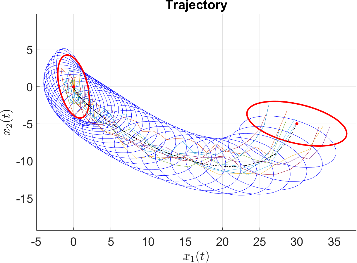
(a) Newton’s method.

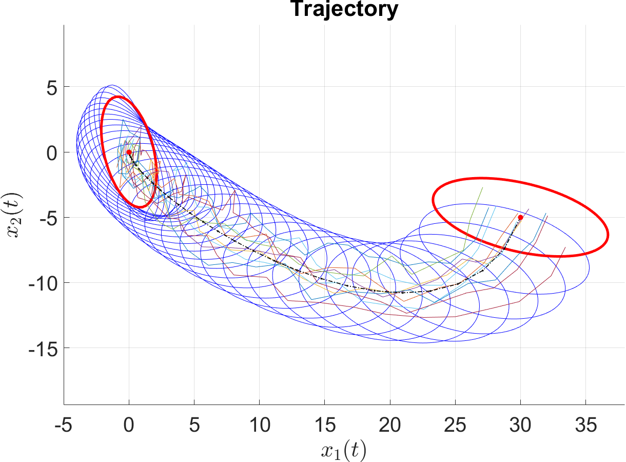
(b) SDP with lossless convex relaxation.

Figure 1: Ten sample paths with the optimal state mean and three-standard-deviation tolerance region.

As expected, the two solutions are identical. For random systems of higher dimensions and longer time horizons, it is observed that Newton’s method is very sensitive to the initialization and does not scale well, and the SDP method is more scalable before it runs out of memory.

VI Concluding Remarks

We have established the existence and uniqueness of the optimal control for the covariance steering of a discrete-time linear stochastic system. We have also shown the separation of the optimal mean and covariance steering problems, and have demonstrated that the exact covariance steering problem can be recast as a convex semi-definite programming problem, which can be solved efficiently using standard convex solvers. In the process, we have investigated various properties of a matrix Riccati difference equation that shows up in the solution for the optimal control. In the future, we would like to study the optimal covariance steering problem for stochastic systems subject to multiplicative noise and chance constraints, and to develop efficient data-driven algorithms for estimating the noise covariance in real-life engineering problems.

Appendix A

Lemma 2.

Suppose Assumption 1, Assumption 2, and Property 1 hold. Then,

$$\sum_{i=0}^{N-1}\Phi_{\bar{A}}(N,i+1)B_{i}\big{(}R_{i}+B_{i}^{\mbox{\tiny\sf T}}\Pi_{i+1}B_{i}\big{)}^{-1}B_{i}^{\mbox{\tiny\sf T}}\Phi_{\bar{A}}(N,i+1)^{\mbox{\tiny\sf T}}\succ 0.$$

Proof.

It is clear that

$$\sum_{i=0}^{N-1}\Phi_{\bar{A}}(N,i+1)B_{i}\big{(}R_{i}+B_{i}^{\mbox{\tiny\sf T}}\Pi_{i+1}B_{i}\big{)}^{-1}B_{i}^{\mbox{\tiny\sf T}}\Phi_{\bar{A}}(N,i+1)^{\mbox{\tiny\sf T}}=\Xi\Lambda\Xi^{\mbox{\tiny\sf T}},$$

where $\Xi\triangleq\big{[}B_{N-1}\qquad\bar{A}_{N-1}B_{N-2}\qquad\cdots\qquad\bar{A}_{N-1}\bar{A}_{N-2}\cdots\bar{A}_{1}B_{0}\big{]}$ and

$$\Lambda\triangleq\operatorname{blkdiag}\!\Big{[}\!\big{(}R_{N-1}+B_{N-1}^{\mbox{\tiny\sf T}}\Pi_{N}B_{N-1}\big{)}^{-1},\big{(}R_{N-2}+B_{N-2}^{\mbox{\tiny\sf T}}\Pi_{N-1}B_{N-2}\big{)}^{-1},\dots,\big{(}R_{0}+B_{0}^{\mbox{\tiny\sf T}}\Pi_{1}B_{0}\big{)}^{-1}\Big{]}.$$

From Property 1, $\Lambda\succ 0$. Thus, it suffices to show that ${\rm rank\;}\Xi=n$. From Assumption 2, the reachability Gramian $G(N,0)\succ 0$. From the Woodbury formula [25], we can write $\bar{A}_{k}=A_{k}+B_{k}F_{k}$ for some $F_{k}\in\mathbb{R}^{p\times n}$. It follows that

$$\operatorname{range}\Xi=\operatorname{range}\Big{[}B_{N-1}\qquad A_{N-1}B_{N-2}\qquad\cdots\qquad A_{N-1}A_{N-2}\cdots A_{1}B_{0}\Big{]}=\mathbb{R}^{n}.$$

Therefore, ${\rm rank\;}\Xi=n$.  

Appendix B

In this appendix, we give the proofs of Proposition 2 and Corollary 1 in Section III-B, along with some related results that are used later to prove Theorem 2. We start with a result that helps us establish the uniqueness of the solution to the Riccati difference equation (5a).

Proposition 6.

If, for a given initial condition $\Pi_{0}$, equation (5a) has a solution from time $0$ to $N$, then, this solution is unique.

Proof.

Let $\mathcal{S}_{n}$ be the set of $n\times n$ symmetric matrices. In view of (5a), it suffices to show that the map $g:\{\Pi\,|\,\Pi\in\mathcal{S}_{n},~{}I_{n}+BB^{\mbox{\tiny\sf T}}\Pi~{}\text{is invertible}\}\to\mathcal{S}_{n}$ with $B\in\mathbb{R}^{n\times p}$, defined by

$$g:\Pi\mapsto\Pi\big{(}I_{n}+BB^{\mbox{\tiny\sf T}}\Pi\big{)}^{-1},$$

is injective.

Suppose $H=g(\Pi)$ for some $\Pi$. If $H$ is invertible, then $\Pi$ must be invertible. It follows that $H=\big{(}\Pi^{-1}+BB^{\mbox{\tiny\sf T}}\big{)}^{-1}$. Then, $\Pi=\big{(}H^{-1}-BB^{\mbox{\tiny\sf T}}\big{)}^{-1}$ is unique.

If $H$ is singular, then any $\Pi$ that satisfies $H=g(\Pi)$ must be singular. Moreover, for any such $\Pi$, we have $\ker H=\ker\Pi$, since, for some $z\in\mathbb{R}^{n}$, $z^{\mbox{\tiny\sf T}}H=0$ if and only if $z^{\mbox{\tiny\sf T}}\Pi=0$. Hence, we can quotient out the common kernel of $H$ and $\Pi$. Since $H,\Pi\in\mathcal{S}_{n}$, there exists an $n\times n$ orthogonal matrix $V\triangleq[\bar{V}\enspace\tilde{V}]$ such that

$$H=\begin{bmatrix}\bar{V}&\tilde{V}\end{bmatrix}\begin{bmatrix}\bar{\Lambda}&0\\ 0&0\end{bmatrix}\begin{bmatrix}\bar{V}^{\mbox{\tiny\sf T}}\\ \tilde{V}^{\mbox{\tiny\sf T}}\end{bmatrix},\quad\Pi=\begin{bmatrix}\bar{V}&\tilde{V}\end{bmatrix}\begin{bmatrix}\bar{\Pi}&0\\ 0&0\end{bmatrix}\begin{bmatrix}\bar{V}^{\mbox{\tiny\sf T}}\\ \tilde{V}^{\mbox{\tiny\sf T}}\end{bmatrix},$$

where $\ker H=\ker\Pi=\operatorname{range}\tilde{V}$ and $\bar{\Lambda}$ is an $r\times r$ diagonal matrix. It can be checked that $\bar{\Lambda}=\bar{\Pi}\big{(}I_{r}+T\bar{\Pi}\big{)}^{-1}$, where $T$ is the $r$th leading principal submatrix (that is, the upper-left $r\times r$ submatrix) of $V^{\mbox{\tiny\sf T}}BB^{\mbox{\tiny\sf T}}V$. Since $\bar{\Pi}$ is invertible by construction, we have $\bar{\Lambda}=\big{(}\bar{\Pi}^{-1}+T\big{)}^{-1}$. Thus, $\bar{\Pi}$ is unique. It follows immediately that $\Pi$ is also unique.  

We are now ready to provide the proof of Proposition 2.

Proof of Proposition 2.

(Sufficiency) Suppose, for all $k=0,1,\dots,N$, the matrix $\Phi_{11}(k,0)+\Phi_{12}(k,0)\Pi_{0}$ is invertible. We will show that the matrix $\Pi_{k}$ given by (18) is a solution of (5a). Since $\Phi_{M}(k+1,0)=M_{k}\Phi_{M}(k,0)$, it follows that

$$\begin{bmatrix}\Phi_{11}(k,0)+\Phi_{12}(k,0)\Pi_{0}\\ \Phi_{21}(k,0)+\Phi_{22}(k,0)\Pi_{0}\end{bmatrix}=M_{k}^{-1}\begin{bmatrix}\Phi_{11}(k+1,0)+\Phi_{12}(k+1,0)\Pi_{0}\\ \Phi_{21}(k+1,0)+\Phi_{22}(k+1,0)\Pi_{0}\end{bmatrix}.$$ (38)

Moreover, we can compute that

$$M_{k}^{-1}=\begin{bmatrix}A_{k}^{-1}&A_{k}^{-1}B_{k}B_{k}^{\mbox{\tiny\sf T}}\\ Q_{k}A_{k}^{-1}&A_{k}^{\mbox{\tiny\sf T}}+Q_{k}A_{k}^{-1}B_{k}B_{k}^{\mbox{\tiny\sf T}}\end{bmatrix}.$$ (39)

Putting (38) and (39) together, it can be checked that the $\Pi_{k}$ given by (18) satisfies (5a).

(Necessity) Suppose (5a) has a solution from time $0$ to $N$, denoted by $\Pi_{k}$. From Proposition 6, the solution is unique. Clearly, $\Phi_{11}(0,0)+\Phi_{12}(0,0)\Pi_{0}=I_{n}$ is invertible. Assume that there exists $0\leq k\leq N-1$ such that, for all $i=0,1,\dots,k$, the matrix $\Phi_{11}(i,0)+\Phi_{12}(i,0)\Pi_{0}$ is invertible, but the matrix $\Phi_{11}(k+1,0)+\Phi_{12}(k+1,0)\Pi_{0}$ is singular. In view of the proof for sufficiency, the unique solution of (5a) up to time $k$ is given by (18). From (5a), and since $A_{k}$ is invertible and $\Pi_{k}$ is symmetric,

$$\Pi_{k} =A_{k}^{\mbox{\tiny\sf T}}\Pi_{k+1}\big{(}I_{n}+B_{k}B_{k}^{\mbox{\tiny\sf T}}\Pi_{k+1}\big{)}^{-1}A_{k}+Q_{k}$$

$$=\Big{(}A_{k}^{\mbox{\tiny\sf T}}\Pi_{k+1}+Q_{k}\big{(}A_{k}^{-1}+A_{k}^{-1}B_{k}B_{k}^{\mbox{\tiny\sf T}}\Pi_{k+1}\big{)}\Big{)}\Big{(}A_{k}^{-1}+A_{k}^{-1}B_{k}B_{k}^{\mbox{\tiny\sf T}}\Pi_{k+1}\Big{)}^{-1}$$

$$=\Big{(}A_{k}^{-\mbox{\tiny\sf T}}+\Pi_{k+1}B_{k}B_{k}^{\mbox{\tiny\sf T}}A_{k}^{-\mbox{\tiny\sf T}}\Big{)}^{-1}\Big{(}\Pi_{k+1}A_{k}+\big{(}A_{k}^{-\mbox{\tiny\sf T}}+\Pi_{k+1}B_{k}B_{k}^{\mbox{\tiny\sf T}}A_{k}^{-\mbox{\tiny\sf T}}\big{)}Q_{k}\Big{)}.$$

From (18) and (38),

$$\Pi_{k} =\Big{(}\Phi_{21}(k,0)+\Phi_{22}(k,0)\Pi_{0}\Big{)}\Big{(}\Phi_{11}(k,0)+\Phi_{12}(k,0)\Pi_{0}\Big{)}^{-1}$$

$$=\Big{(}Q_{k}A_{k}^{-1}\Big{[}\Phi_{11}(k+1,0)+\Phi_{12}(k+1,0)\Pi_{0}\Big{]}$$

$$\hskip 56.9055pt+\big{(}A_{k}^{\mbox{\tiny\sf T}}+Q_{k}A_{k}^{-1}B_{k}B_{k}^{\mbox{\tiny\sf T}}\big{)}\Big{[}\Phi_{21}(k+1,0)+\Phi_{22}(k+1,0)\Pi_{0}\Big{]}\Big{)}$$

$$\hskip 17.07164pt\times\Big{(}A_{k}^{-1}\Big{[}\Phi_{11}(k+1,0)+\Phi_{12}(k+1,0)\Pi_{0}\Big{]}$$

$$\hskip 56.9055pt+A_{k}^{-1}B_{k}B_{k}^{\mbox{\tiny\sf T}}\Big{[}\Phi_{21}(k+1,0)+\Phi_{22}(k+1,0)\Pi_{0}\Big{]}\Big{)}^{-1}.$$

Equating the above two equations and canceling out the common terms yield

$$\Phi_{21}(k+1,0)+\Phi_{22}(k+1,0)\Pi_{0}=\Pi_{k+1}\Big{(}\Phi_{11}(k+1,0)+\Phi_{12}(k+1,0)\Pi_{0}\Big{)}.$$

There exists $\Pi_{k+1}$ such that the above equation holds if and only if

$$0\neq\ker\Big{(}\Phi_{11}(k+1,0)+\Phi_{12}(k+1,0)\Pi_{0}\Big{)}\subseteq\ker\Big{(}\Phi_{21}(k+1,0)+\Phi_{22}(k+1,0)\Pi_{0}\Big{)}.$$

It follows that there exists $\xi\in\mathbb{R}^{n}$ with $\xi\neq 0$ such that the right-hand side of (38) times $\xi$ equals zero. However, the left-hand side of (38) times $\xi$ is nonzero, since $\Phi_{11}(k,0)+\Phi_{12}(k,0)\Pi_{0}$ is invertible. We have thus reached a contradiction.  

Proof of Corollary 1.

We will prove (19) by induction. For $\ell=0$, we know that (19) holds because of (18). Assume that, for $\ell=i$, where $i\leq N-1$, (19) holds. It can be checked that $\Phi_{M}(k,i)=\Phi_{M}(k,i+1)M_{i}$ regardless of $i<k$ or $i\geq k$. Then, we have

$$\Pi_{k}=\Big{(}\Phi_{21}(k,i)+\Phi_{22}(k,i)\Pi_{i}\Big{)}\Big{(}\Phi_{11}(k,i)+\Phi_{12}(k,i)\Pi_{i}\Big{)}^{-1}$$

$$=\Big{(}\Phi_{21}(k,i+1)\big{(}A_{i}-B_{i}B_{i}^{\mbox{\tiny\sf T}}A_{i}^{-\mbox{\tiny\sf T}}(\Pi_{i}-Q_{i})\big{)}+\Phi_{22}(k,i+1)\big{(}A_{i}^{-\mbox{\tiny\sf T}}(\Pi_{i}-Q_{i})\big{)}\Big{)}$$

$$\hskip 56.9055pt\times\Big{(}\Phi_{11}(k,i+1)\big{(}A_{i}-B_{i}B_{i}^{\mbox{\tiny\sf T}}A_{i}^{-\mbox{\tiny\sf T}}(\Pi_{i}-Q_{i})\big{)}+\Phi_{12}(k,i+1)\big{(}A_{i}^{-\mbox{\tiny\sf T}}(\Pi_{i}-Q_{i})\big{)}\Big{)}^{-1}$$

$$=\Big{(}\Phi_{21}(k,i+1)+\Phi_{22}(k,i+1)\Pi_{i+1}\Big{)}\Big{(}I_{n}+B_{i}B_{i}^{\mbox{\tiny\sf T}}\Pi_{i+1}\Big{)}^{-1}$$

$$\hskip 56.9055pt\times\Big{(}I_{n}+B_{i}B_{i}^{\mbox{\tiny\sf T}}\Pi_{i+1}\Big{)}\Big{(}\Phi_{11}(k,i+1)+\Phi_{12}(k,i+1)\Pi_{i+1}\Big{)}^{-1}$$

$$=\Big{(}\Phi_{21}(k,i+1)+\Phi_{22}(k,i+1)\Pi_{i+1}\Big{)}\Big{(}\Phi_{11}(k,i+1)+\Phi_{12}(k,i+1)\Pi_{i+1}\Big{)}^{-1}.$$

Thus, for $\ell=i+1$, (19) holds.  

The following auxiliary result is used to show the monotonicity of the solution to (5a) and of the matrix $W_{k,0}$ defined by (24).

Lemma 3.

Let $X\succ 0$ be a $j\times j$ matrix, written as

$$X\triangleq\begin{bmatrix}X_{1}&X_{2}\\ X_{2}^{\mbox{\tiny\sf T}}&X_{4}\end{bmatrix}\succ 0,$$

where $X_{1}$ is an $i\times i$ matrix for some $i<j$. Let $Y$ be an $i\times i$ symmetric matrix. Then,

$$X^{-1}=\begin{bmatrix}X_{1}&X_{2}\\ X_{2}^{\mbox{\tiny\sf T}}&X_{4}\end{bmatrix}^{-1}\succ~{}(\text{respectively},\,\succeq)\begin{bmatrix}Y&0\\ 0&0\end{bmatrix}\quad\iff\quad X_{1}^{-1}\succ~{}(\text{respectively},\,\succeq)~{}Y.$$

Proof.

The fact of $X\succ 0$ implies that $X_{1}\succ 0$ and its Schur complement $X/X_{1}\triangleq X_{4}-X_{2}^{\mbox{\tiny\sf T}}X_{1}^{-1}X_{2}\succ 0$ [25]. Using the expression for $X^{-1}$, we get

$$Z\triangleq X^{-1}-\begin{bmatrix}Y&0\\ 0&0\end{bmatrix}=\begin{bmatrix}X_{1}^{-1}+X_{1}^{-1}X_{2}(X/X_{1})^{-1}X_{2}^{\mbox{\tiny\sf T}}X_{1}^{-1}-Y&-X_{1}^{-1}X_{2}(X/X_{1})^{-1}\\ -(X/X_{1})^{-1}X_{2}^{\mbox{\tiny\sf T}}X_{1}^{-1}&(X/X_{1})^{-1}\end{bmatrix}.$$

We can check that the Schur complement of $(X/X_{1})^{-1}$ in $Z$ is $X_{1}^{-1}-Y$. Since $(X/X_{1})^{-1}\succ 0$, it follows that $Z\succ 0$ (respectively, $Z\succeq 0$) if and only if the Schur complement $X_{1}^{-1}-Y\succ 0$ (respectively, $X_{1}^{-1}-Y\succeq 0$).  

The next result on the monotonicity of the solution to (5a) is used to establish the invertibility of $\Phi_{11}$ in Lemma 5.

Proposition 7.

Let $P_{k}^{1}$ and $P_{k}^{2}$ be the respective solutions to the following Riccati difference equations

$$P_{k}^{1} =A_{k}^{\mbox{\tiny\sf T}}P_{k+1}^{1}\big{(}I_{n}+\Upsilon_{k}P_{k+1}^{1}\big{)}^{-1}A_{k}+\Omega_{k},\quad P_{0}^{1}=0_{n\times n},$$

$$P_{k}^{2} =A_{k}^{\mbox{\tiny\sf T}}P_{k+1}^{2}\big{(}I_{n}+\Gamma_{k}P_{k+1}^{2}\big{)}^{-1}A_{k}+Q_{k},\quad P_{0}^{2}=0_{n\times n},$$

where $A_{k}$ is invertible and $\Upsilon_{k},\Gamma_{k},\Omega_{k},Q_{k}\succeq 0$ over the maximal integer time intervals of existence of the respective solutions $P_{k}^{1}$ and $P_{k}^{2}$. Let $\mathcal{I}\subseteq\mathbb{Z}$ denote the common integer time intervals of existence of $P_{k}^{1}$ and $P_{k}^{2}$. If, for all $k\in\mathcal{I}$, $\Omega_{k}\succeq Q_{k}$ and $\Upsilon_{k}\preceq\Gamma_{k}$, then,

$$P_{k}^{1}\succeq P_{k}^{2}\succeq 0,\quad k\in\mathcal{I},~{}k\leq 0,$$ (40a)

$$P_{k}^{1}\preceq P_{k}^{2}\preceq 0,\quad k\in\mathcal{I},~{}k\geq 0.$$ (40b)

Proof.

For the case $k\leq 0$, (40a) follows directly from [32]. We will prove (40b) by induction. To this end, $P_{0}^{1}=P_{0}^{2}=0$, thus, for $k=0$, (40b) holds. Assume, for $k=i\geq 0$, (40b) holds. We will show that, for $k=i+1\in\mathcal{I}$, (40b) also holds. Since $\Omega_{i}\succeq Q_{i}$, we have

$$P_{i+1}^{1}\big{(}I_{n}+\Upsilon_{i}P_{i+1}^{1}\big{)}^{-1}\preceq P_{i+1}^{2}\big{(}I_{n}+\Gamma_{i}P_{i+1}^{2}\big{)}^{-1}\preceq 0.$$ (41)

Let $z\in\ker P_{i+1}^{1}$, that is, $P_{i+1}^{1}z=0$. Since $P_{i+1}^{1}$ is symmetric, it follows that $z^{\mbox{\tiny\sf T}}P_{i+1}^{1}=0$. In light of (41), we have $0=z^{\mbox{\tiny\sf T}}P_{i+1}^{1}\big{(}I_{n}+\Upsilon_{i}P_{i+1}^{1}\big{)}^{-1}z\leq z^{\mbox{\tiny\sf T}}P_{i+1}^{2}\big{(}I_{n}+\Gamma_{i}P_{i+1}^{2}\big{)}^{-1}z\leq 0$. Hence, $z^{\mbox{\tiny\sf T}}P_{i+1}^{2}\big{(}I_{n}+\Gamma_{i}P_{i+1}^{2}\big{)}^{-1}z=0$. Since $P_{i+1}^{2}\big{(}I_{n}+\Gamma_{i}P_{i+1}^{2}\big{)}^{-1}\preceq 0$, it must be true that $z^{\mbox{\tiny\sf T}}P_{i+1}^{2}\big{(}I_{n}+\Gamma_{i}P_{i+1}^{2}\big{)}^{-1}=0$. Since $\big{(}I_{n}+\Gamma_{i}P_{i+1}^{2}\big{)}^{-1}$ is invertible, it follows that $z^{\mbox{\tiny\sf T}}P_{i+1}^{2}=0$. Since $P_{i+1}^{2}$ is symmetric, we have $z\in\ker P_{i+1}^{2}$. It follows that $\ker P_{i+1}^{1}\subseteq\ker P_{i+1}^{2}$.

If $P_{i+1}^{1}$ and $P_{i+1}^{2}$ are invertible, it follows that $\Big{(}\big{(}P_{i+1}^{1}\big{)}^{-1}+\Upsilon_{i}\Big{)}^{-1}\preceq\Big{(}\big{(}P_{i+1}^{2}\big{)}^{-1}+\Gamma_{i}\Big{)}^{-1}\prec 0$. Hence, $\big{(}P_{i+1}^{2}\big{)}^{-1}+\Gamma_{i}\preceq\big{(}P_{i+1}^{1}\big{)}^{-1}+\Upsilon_{i}\prec 0$. Since $\Gamma_{k}\succeq\Upsilon_{k}\succeq 0$, it follows that $\big{(}P_{i+1}^{2}\big{)}^{-1}\preceq\big{(}P_{i+1}^{1}\big{)}^{-1}\prec 0$. Thus, we have $P_{i+1}^{1}\preceq P_{i+1}^{2}\prec 0$.

Without loss of generality, assume $P_{i+1}^{1}$ and $P_{i+1}^{2}$ are singular and $\ker P_{i+1}^{1}$ is a proper subset of $\ker P_{i+1}^{2}$. The cases when $P_{i+1}^{1}$ is invertible and $P_{i+1}^{2}$ is singular or when $\ker P_{i+1}^{1}=\ker P_{i+1}^{2}$ can be proved in a similar way. Since $\ker P_{i+1}^{1}\subseteq\ker P_{i+1}^{2}$, there exists an $n\times n$ orthogonal matrix $U\triangleq[\bar{U}\enspace\tilde{U}]$ such that

$$P_{i+1}^{1}=\begin{bmatrix}\bar{U}&\tilde{U}\end{bmatrix}\begin{bmatrix}\bar{P}^{1}&0\\ 0&0\end{bmatrix}\begin{bmatrix}\bar{U}^{\mbox{\tiny\sf T}}\\ \tilde{U}^{\mbox{\tiny\sf T}}\end{bmatrix},\quad P_{i+1}^{2}=\begin{bmatrix}\bar{U}&\tilde{U}\end{bmatrix}\begin{bmatrix}\bar{P}^{2}&0\\ 0&0\end{bmatrix}\begin{bmatrix}\bar{U}^{\mbox{\tiny\sf T}}\\ \tilde{U}^{\mbox{\tiny\sf T}}\end{bmatrix},$$

where $\ker P_{i+1}^{1}=\operatorname{range}\tilde{U}$ and $\bar{P}^{1}$ is an $r\times r$ diagonal matrix. It suffices to show that $\bar{P}^{1}\preceq\bar{P}^{2}\preceq 0$.

Since $\ker P_{i+1}^{1}\neq\ker P_{i+1}^{2}$, there exists an $r\times r$ orthogonal matrix $V\triangleq[\hat{V}\enspace\tilde{V}]$ such that

$$\bar{P}^{2}=\begin{bmatrix}\hat{V}&\tilde{V}\end{bmatrix}\begin{bmatrix}\hat{P}^{2}&0\\ 0&0\end{bmatrix}\begin{bmatrix}\hat{V}^{\mbox{\tiny\sf T}}\\ \tilde{V}^{\mbox{\tiny\sf T}}\end{bmatrix},$$

where $\ker\bar{P}^{2}=\operatorname{range}\tilde{V}$ and $\hat{P}^{2}$ is an $\rho\times\rho$ diagonal matrix. To this end, it suffices to show that

$$V^{\mbox{\tiny\sf T}}\bar{P}^{1}V\preceq\begin{bmatrix}\hat{P}^{2}&0\\ 0&0\end{bmatrix}\preceq 0.$$

Multiplying (41) by $U^{\mbox{\tiny\sf T}}$ on the left and by $U$ on the right yields the matrix inequality

$$\Big{(}\big{(}\bar{P}^{1}\big{)}^{-1}+\bar{\Upsilon}\Big{)}^{-1}=\bar{P}^{1}\big{(}I_{r}+\bar{\Upsilon}\bar{P}^{1}\big{)}^{-1}\preceq\bar{P}^{2}\big{(}I_{r}+\bar{\Gamma}\bar{P}^{2}\big{)}^{-1}\preceq 0,$$ (42)

where $\bar{\Upsilon}$ and $\bar{\Gamma}$ are the $r$th leading principal submatrices of $U^{\mbox{\tiny\sf T}}\Upsilon_{i}U$ and $U^{\mbox{\tiny\sf T}}\Gamma_{i}U$, respectively. Multiplying (42) by $V^{\mbox{\tiny\sf T}}$ on the left and by $V$ on the right yields

$$\Big{(}V^{\mbox{\tiny\sf T}}\big{(}\bar{P}^{1}\big{)}^{-1}V+V^{\mbox{\tiny\sf T}}\bar{\Upsilon}V\Big{)}^{-1}\preceq\begin{bmatrix}\Big{(}\big{(}\hat{P}^{2}\big{)}^{-1}+\hat{\Gamma}\Big{)}^{-1}&0\\ 0&0\end{bmatrix}\preceq 0,$$ (43)

where $\hat{\Gamma}$ is the $\rho$th leading principal submatrix of $V^{\mbox{\tiny\sf T}}\bar{\Gamma}V$. Let

$$V^{\mbox{\tiny\sf T}}\big{(}\bar{P}^{1}\big{)}^{-1}V\triangleq\begin{bmatrix}\hat{Z}&\hat{Z}_{2}\\ \hat{Z}_{2}^{\mbox{\tiny\sf T}}&\hat{Z}_{4}\end{bmatrix},\quad V^{\mbox{\tiny\sf T}}\bar{\Upsilon}V\triangleq\begin{bmatrix}\hat{\Upsilon}&\hat{\Upsilon}_{2}\\ \hat{\Upsilon}_{2}^{\mbox{\tiny\sf T}}&\hat{\Upsilon}_{4}\end{bmatrix}.$$

Since $\Big{(}V^{\mbox{\tiny\sf T}}\big{(}\bar{P}^{1}\big{)}^{-1}V+V^{\mbox{\tiny\sf T}}\bar{\Upsilon}V\Big{)}^{-1}\prec 0$, the matrix inequality (43) and Lemma 3 imply that

$$\big{(}\hat{Z}+\hat{\Upsilon}\big{)}^{-1}\preceq\Big{(}\big{(}\hat{P}^{2}\big{)}^{-1}+\hat{\Gamma}\Big{)}^{-1}\prec 0.$$

It follows that $\big{(}\hat{P}^{2}\big{)}^{-1}+\hat{\Gamma}\preceq\hat{Z}+\hat{\Upsilon}\prec 0$. Since $\hat{\Gamma}\succeq\hat{\Upsilon}\succeq 0$, it follows that $\big{(}\hat{P}^{2}\big{)}^{-1}\preceq\hat{Z}\prec 0$. Thus, we have $\hat{Z}^{-1}\preceq\hat{P}^{2}\prec 0$. The fact that $\Big{(}V^{\mbox{\tiny\sf T}}\big{(}\bar{P}^{1}\big{)}^{-1}V+V^{\mbox{\tiny\sf T}}\bar{\Upsilon}V\Big{)}^{-1}\prec 0$ implies that $V^{\mbox{\tiny\sf T}}\bar{P}^{1}V\prec 0$. It then follows from Lemma 3 that

$$V^{\mbox{\tiny\sf T}}\bar{P}^{1}V=\begin{bmatrix}\hat{Z}&\hat{Z}_{2}\\ \hat{Z}_{2}^{\mbox{\tiny\sf T}}&\hat{Z}_{4}\end{bmatrix}^{-1}\preceq\begin{bmatrix}\hat{P}^{2}&0\\ 0&0\end{bmatrix}\preceq 0.$$

This completes the proof.  

Appendix C

In this appendix, we present some useful properties of the state transition matrix $\Phi_{M}$ defined by (17). These properties are used to prove Theorem 1, Theorem 2, and Theorem 3.

Let

$$\Phi_{M}(k,s)^{-1}=\Phi_{M}(s,k)\triangleq\begin{bmatrix}\Phi_{11}(s,k)&\Phi_{12}(s,k)\\ \Phi_{21}(s,k)&\Phi_{22}(s,k)\end{bmatrix}.$$

Lemma 4.

If, for all $k\in\mathbb{Z}$, $A_{k}$ is invertible, then, for all $k,s\in\mathbb{Z}$,

$$\Phi_{12}(k,s)^{\mbox{\tiny\sf T}}\Phi_{22}(k,s) =\Phi_{22}(k,s)^{\mbox{\tiny\sf T}}\Phi_{12}(k,s),$$ (44a)

$$\Phi_{21}(k,s)^{\mbox{\tiny\sf T}}\Phi_{11}(k,s) =\Phi_{11}(k,s)^{\mbox{\tiny\sf T}}\Phi_{21}(k,s),$$ (44b)

$$\Phi_{12}(k,s)\Phi_{11}(k,s)^{\mbox{\tiny\sf T}} =\Phi_{11}(k,s)\Phi_{12}(k,s)^{\mbox{\tiny\sf T}},$$ (44c)

$$\Phi_{21}(k,s)\Phi_{22}(k,s)^{\mbox{\tiny\sf T}} =\Phi_{22}(k,s)\Phi_{21}(k,s)^{\mbox{\tiny\sf T}},$$ (44d)

$$\Phi_{11}(k,s)^{\mbox{\tiny\sf T}}\Phi_{22}(k,s) -\Phi_{21}(k,s)^{\mbox{\tiny\sf T}}\Phi_{12}(k,s)=I_{n},$$ (44e)

$$\Phi_{11}(k,s)\Phi_{22}(k,s)^{\mbox{\tiny\sf T}} -\Phi_{12}(k,s)\Phi_{21}(k,s)^{\mbox{\tiny\sf T}}=I_{n}.$$ (44f)

Proof.

When $s=k$, $\Phi_{11}(s,s)=\Phi_{22}(s,s)=I_{n}$ and $\Phi_{12}(s,s)=\Phi_{21}(s,s)=0$. Clearly, for $s=k$, Lemma 4 holds. Let

$$\bar{J}\triangleq\begin{bmatrix}0&I_{n}\\ -I_{n}&0\end{bmatrix}.$$

It can be checked that $M_{k}^{\mbox{\tiny\sf T}}\bar{J}M_{k}=\bar{J}=M_{k}\bar{J}M_{k}^{\mbox{\tiny\sf T}}$.

When $s<k$, $\Phi_{M}(k,s)=M_{k-1}\Phi_{M}(k-1,s)$. It follows immediately that $\Phi_{M}(k,s)^{\mbox{\tiny\sf T}}\bar{J}\Phi_{M}(k,s)=\Phi_{M}(k-1,s)^{\mbox{\tiny\sf T}}M_{k-1}^{\mbox{\tiny\sf T}}\bar{J}M_{k-1}\Phi_{M}(k-1,s)=\Phi_{M}(k-1,s)^{\mbox{\tiny\sf T}}\bar{J}\Phi_{M}(k-1,s)$. Since, for all $s<k$, the above equation holds, by induction, we have $\Phi_{M}(k,s)^{\mbox{\tiny\sf T}}\bar{J}\Phi_{M}(k,s)=\Phi_{M}(s,s)^{\mbox{\tiny\sf T}}\bar{J}\Phi_{M}(s,s)=\bar{J}$. Similarly,

$$\Phi_{M}(k,s)\bar{J}\Phi_{M}(k,s)^{\mbox{\tiny\sf T}} =M_{k-1}\Phi_{M}(k-1,s)\bar{J}\Phi_{M}(k-1,s)^{\mbox{\tiny\sf T}}M_{k-1}^{\mbox{\tiny\sf T}}$$

$$=M_{k-1}\cdots M_{s}\Phi_{M}(s,s)\bar{J}\Phi_{M}(s,s)^{\mbox{\tiny\sf T}}M_{s}^{\mbox{\tiny\sf T}}\cdots M_{k-1}^{\mbox{\tiny\sf T}}=\bar{J}.$$

Thus, for $s<k$, Lemma 4 holds. Similarly, it can be shown that, for $s>k$, Lemma 4 holds.  

The next result establishes the invertibility of $\Phi_{11}$.

Lemma 5.

If, for all $k\in\mathbb{Z}$, $A_{k}$ is invertible, then, for all $k,s\in\mathbb{Z}$, $\Phi_{11}(k,s)$ and $\Phi_{22}(k,s)$ are invertible. In particular,

$$\Phi_{11}(k,s) =\Phi_{22}(s,k)^{\mbox{\tiny\sf T}}$$ (45)

$$=\Big{(}\Phi_{11}(s,k)-\Phi_{12}(s,k)\Phi_{22}(s,k)^{-1}\Phi_{21}(s,k)\Big{)}^{-1}$$

$$=\Big{(}\Phi_{22}(k,s)^{\mbox{\tiny\sf T}}-\Phi_{12}(k,s)^{\mbox{\tiny\sf T}}\Phi_{11}(k,s)^{-\mbox{\tiny\sf T}}\Phi_{21}(k,s)^{\mbox{\tiny\sf T}}\Big{)}^{-1}.$$

Proof.

First, we show that $\Phi_{11}(k,s)$ is invertible. Let $\Pi_{k}$ be the solution to (5a) with $\Pi_{0}=0_{n\times n}$, and let $\mathcal{I}_{0}\subseteq\mathbb{Z}$ be the maximal integer time interval of existence of $\Pi_{k}$. Let $\bar{\Pi}_{k}$ be the solution to (5a) when $Q_{k}\equiv 0_{n\times n}$ and $\bar{\Pi}_{0}=0_{n\times n}$. Clearly, we have, for all $k\in\mathbb{Z}$, $\bar{\Pi}_{k}\equiv 0_{n\times n}$. Let $\hat{\Pi}_{k}$ be the solution to (5a) when $B_{k}\equiv 0_{n\times n}$ and $\hat{\Pi}_{0}=0_{n\times n}$. Since when $B_{k}\equiv 0_{n\times n}$, (5a) is a linear matrix equation, it follows that, for all $k\in\mathbb{Z}$, the solution $\hat{\Pi}_{k}$ exists. Moreover, it is easy to see that, for $k<0$, $\hat{\Pi}_{k}\succeq 0$, and, for $k>0$, $\hat{\Pi}_{k}\preceq 0$.

From the monotonicity of the matrix Riccati difference equation in Proposition 7, we have

$$0\equiv\bar{\Pi}_{k}\preceq\Pi_{k}\preceq\hat{\Pi}_{k},\quad k\in\mathcal{I}_{0},~{}k\leq 0,$$

$$\hat{\Pi}_{k}\preceq\Pi_{k}\preceq\bar{\Pi}_{k}\equiv 0,\quad k\in\mathcal{I}_{0},~{}k\geq 0.$$

Hence, $\Pi_{k}$ has no finite escape time and $\mathcal{I}_{0}=\mathbb{Z}$. From Proposition 2, for all $k\in\mathbb{Z}$, $\Phi_{11}(k,0)$ is invertible. A similar argument shows that, for all $k,s\in\mathbb{Z}$, $\Phi_{11}(k,s)$ is invertible.

Next, we show that $\Phi_{11}(k,s)=\Phi_{22}(s,k)^{\mbox{\tiny\sf T}}$. From (44f) and (44c), it follows that

$$\Phi_{11}(k,s)^{-1} =\Phi_{22}(k,s)^{\mbox{\tiny\sf T}}-\Phi_{11}(k,s)^{-1}\Phi_{12}(k,s)\Phi_{21}(k,s)^{\mbox{\tiny\sf T}}$$

$$=\Phi_{22}(k,s)^{\mbox{\tiny\sf T}}-\Phi_{12}(k,s)^{\mbox{\tiny\sf T}}\Phi_{11}(k,s)^{-\mbox{\tiny\sf T}}\Phi_{21}(k,s)^{\mbox{\tiny\sf T}}.$$

Since $\Phi_{11}(k,s)$ is invertible, the Schur complement of block $\Phi_{11}(k,s)$ in the matrix $\Phi_{M}(k,s)$ is given by $\Phi_{22}(k,s)-\Phi_{21}(k,s)\Phi_{11}(k,s)^{-1}\Phi_{12}(k,s)=\Phi_{22}(s,k)^{-1}$. Therefore, we have $\Phi_{11}(k,s)=\Phi_{22}(s,k)^{\mbox{\tiny\sf T}}$. The other equality can be shown analogously.  

Lemma 6.

If, for all $k\in\mathbb{Z}$, $A_{k}$ is invertible, then, for all $k,s\in\mathbb{Z}$,

$$\Phi_{12}(k,s) =-\Phi_{12}(s,k)^{\mbox{\tiny\sf T}},$$ (46a)

$$\Phi_{21}(k,s) =-\Phi_{21}(s,k)^{\mbox{\tiny\sf T}}.$$ (46b)

Proof.

It follows from equation (44c) and Lemma 5 that

$$\Phi_{12}(k,s)=\Phi_{11}(k,s)\Phi_{12}(k,s)^{\mbox{\tiny\sf T}}\Phi_{11}(k,s)^{-\mbox{\tiny\sf T}}=\Phi_{22}(s,k)^{\mbox{\tiny\sf T}}\Phi_{12}(k,s)^{\mbox{\tiny\sf T}}\Phi_{11}(k,s)^{-\mbox{\tiny\sf T}}.$$

Since $\Phi_{M}(k,s)\Phi_{M}(s,k)=I_{2n}$, we have $\Phi_{11}(k,s)\Phi_{12}(s,k)+\Phi_{12}(k,s)\Phi_{22}(s,k)=0$. Thus,

$$-\Phi_{12}(s,k)^{\mbox{\tiny\sf T}}=\Phi_{22}(s,k)^{\mbox{\tiny\sf T}}\Phi_{12}(k,s)^{\mbox{\tiny\sf T}}\Phi_{11}(k,s)^{-\mbox{\tiny\sf T}}=\Phi_{12}(k,s).$$

Similarly, it follows from equation (44d) and Lemma 5 that

$$\Phi_{21}(k,s)=\Phi_{22}(k,s)\Phi_{21}(k,s)^{\mbox{\tiny\sf T}}\Phi_{22}(k,s)^{-\mbox{\tiny\sf T}}=\Phi_{11}(s,k)^{\mbox{\tiny\sf T}}\Phi_{21}(k,s)^{\mbox{\tiny\sf T}}\Phi_{22}(k,s)^{-\mbox{\tiny\sf T}}.$$

Since $\Phi_{21}(k,s)\Phi_{11}(s,k)+\Phi_{22}(k,s)\Phi_{21}(s,k)=0$, it follows that

$$-\Phi_{21}(s,k)^{\mbox{\tiny\sf T}}=\Phi_{11}(s,k)^{\mbox{\tiny\sf T}}\Phi_{21}(k,s)^{\mbox{\tiny\sf T}}\Phi_{22}(k,s)^{-\mbox{\tiny\sf T}}=\Phi_{21}(k,s).$$

This completes the proof.  

Lemma 7.

Under Assumption 1, for all $k=0,1,\dots,N$,

$$\Phi_{21}(k,0)\Phi_{11}(k,0)^{-1}=\Phi_{11}(k,0)^{-\mbox{\tiny\sf T}}\Phi_{21}(k,0)^{\mbox{\tiny\sf T}}\preceq 0.$$

Proof.

From (44b), we have $\Phi_{21}(k,s)^{\mbox{\tiny\sf T}}\Phi_{11}(k,s)=\Phi_{11}(k,s)^{\mbox{\tiny\sf T}}\Phi_{21}(k,s)$. From Lemma 5, $\Phi_{11}(k,s)$ is invertible. It follows that $\Phi_{21}(k,0)\Phi_{11}(k,0)^{-1}=\Phi_{11}(k,0)^{-\mbox{\tiny\sf T}}\Phi_{21}(k,0)^{\mbox{\tiny\sf T}}$.

Now, we show $\Phi_{21}(k,0)\Phi_{11}(k,0)^{-1}\preceq 0$ by induction. When $k=0$, $\Phi_{21}(0,0)\Phi_{11}(0,0)^{-1}=0$. For $k=i$, assume $\Phi_{21}(i,0)\Phi_{11}(i,0)^{-1}\preceq 0$. It follows from $\Phi_{M}(i+1,0)=M_{i}\Phi_{M}(i,0)$ that

$$\Phi_{11}(i+1,0) =A_{i}\Phi_{11}(i,0)+B_{i}B_{i}^{\mbox{\tiny\sf T}}A_{i}^{-\mbox{\tiny\sf T}}\big{(}Q_{i}-\Phi_{21}(i,0)\Phi_{11}(i,0)^{-1}\big{)}\Phi_{11}(i,0),$$ (47a)

$$\Phi_{21}(i+1,0) =-A_{i}^{-\mbox{\tiny\sf T}}\big{(}Q_{i}-\Phi_{21}(i,0)\Phi_{11}(i,0)^{-1}\big{)}\Phi_{11}(i,0).$$ (47b)

Thus, from (47), we have

$$\Phi_{11}(i+1,0)^{\mbox{\tiny\sf T}}\Phi_{21}(i+1,0)=-\Phi_{11}(i,0)^{\mbox{\tiny\sf T}}\big{(}Q_{i}-\Phi_{21}(i,0)\Phi_{11}(i,0)^{-1}\big{)}\Phi_{11}(i,0)$$

$$\hskip 11.38109pt-\Phi_{11}(i,0)^{\mbox{\tiny\sf T}}\big{(}Q_{i}-\Phi_{21}(i,0)\Phi_{11}(i,0)^{-1}\big{)}A_{i}^{-1}B_{i}B_{i}^{\mbox{\tiny\sf T}}A_{i}^{-\mbox{\tiny\sf T}}\big{(}Q_{i}-\Phi_{21}(i,0)\Phi_{11}(i,0)^{-1}\big{)}\Phi_{11}(i,0).$$

Since $\Phi_{21}(i,0)\Phi_{11}(i,0)^{-1}\preceq 0$ and $Q_{i}\succeq 0$, it follows that $\Phi_{11}(i+1,0)^{\mbox{\tiny\sf T}}\Phi_{21}(i+1,0)\preceq 0$. Therefore, it is clear that $\Phi_{21}(i+1,0)\Phi_{11}(i+1,0)^{-1}\preceq 0$.  

The next result plays a critical role in showing Theorem 2 and the positive definiteness of $-\Phi_{11}(N,0)^{-1}\Phi_{12}(N,0)$ in Corollary 3. If, for all $k\in\mathbb{Z}$, $A_{k}$ is invertible, then, it follows from $\Phi_{11}(k,s)\Phi_{12}(s,k)+\Phi_{12}(k,s)\Phi_{22}(s,k)=0$ and Lemma 5 that,

$$-\Phi_{11}(k,s)^{-1}\Phi_{12}(k,s)=\Phi_{12}(s,k)\Phi_{22}(s,k)^{-1},\quad k,s\in\mathbb{Z}.$$

Lemma 8.

Under Assumption 1, for all $k=1,2,\dots,N$,

$$-\Phi_{11}(k,0)^{-1}\Phi_{12}(k,0)=\sum_{i=0}^{k-1}X_{i},$$

where

$$X_{i}\triangleq\Phi_{11}(i,0)^{-1}A_{i}^{-1}B_{i}\Big{(}I_{p}+B_{i}^{\mbox{\tiny\sf T}}A_{i}^{-\mbox{\tiny\sf T}}\big{(}Q_{i}-\Phi_{21}(i,0)\Phi_{11}(i,0)^{-1}\big{)}A_{i}^{-1}B_{i}\Big{)}^{-1}B_{i}^{\mbox{\tiny\sf T}}A_{i}^{-\mbox{\tiny\sf T}}\Phi_{11}(i,0)^{-\mbox{\tiny\sf T}}\succeq 0.$$

Proof.

It follows from Lemma 7 that $X_{i}\succeq 0$. For all $k=0,1,\dots,N-1$, we can compute that,

$$-\Phi_{12}(k+1,0)\Phi_{11}(k,0)^{\mbox{\tiny\sf T}} =-M_{k,1}\Phi_{12}(k,0)\Phi_{11}(k,0)^{\mbox{\tiny\sf T}}-M_{k,2}\Phi_{22}(k,0)\Phi_{11}(k,0)^{\mbox{\tiny\sf T}}$$

$$=-M_{k,1}\Phi_{11}(k,0)\Phi_{12}(k,0)^{\mbox{\tiny\sf T}}-M_{k,2}\Phi_{21}(k,0)\Phi_{12}(k,0)^{\mbox{\tiny\sf T}}-M_{k,2}$$

$$=-\Phi_{11}(k+1,0)\Phi_{12}(k,0)^{\mbox{\tiny\sf T}}-M_{k,2},$$

where $M_{k,1}$ and $M_{k,2}$ are given in (16). In view of Lemma 5 and Lemma 4, we have

$$-\Phi_{11}(k+1,0)^{-1}\Phi_{12}(k+1,0) =-\Phi_{12}(k,0)^{\mbox{\tiny\sf T}}\Phi_{11}(k,0)^{-\mbox{\tiny\sf T}}-\Phi_{11}(k+1,0)^{-1}M_{k,2}\Phi_{11}(k,0)^{-\mbox{\tiny\sf T}}$$

$$=-\Phi_{11}(k,0)^{-1}\Phi_{12}(k,0)+\Phi_{11}(k+1,0)^{-1}B_{k}B_{k}^{\mbox{\tiny\sf T}}A_{k}^{-\mbox{\tiny\sf T}}\Phi_{11}(k,0)^{-\mbox{\tiny\sf T}}.$$

Next, we show that $X_{k}=\Phi_{11}(k+1,0)^{-1}B_{k}B_{k}^{\mbox{\tiny\sf T}}A_{k}^{-\mbox{\tiny\sf T}}\Phi_{11}(k,0)^{-\mbox{\tiny\sf T}}$. It is easy to check that

$$\Big{(}A_{k}+B_{k}B_{k}^{\mbox{\tiny\sf T}}A_{k}^{-\mbox{\tiny\sf T}}\big{(}Q_{k}-\Phi_{21}(k,0)\Phi_{11}(k,0)^{-1}\big{)}\Big{)}A_{k}^{-1}B_{k}$$

$$=B_{k}+B_{k}B_{k}^{\mbox{\tiny\sf T}}A_{k}^{-\mbox{\tiny\sf T}}\big{(}Q_{k}-\Phi_{21}(k,0)\Phi_{11}(k,0)^{-1}\big{)}A_{k}^{-1}B_{k}$$

$$=B_{k}\Big{(}I_{p}+B_{k}^{\mbox{\tiny\sf T}}A_{k}^{-\mbox{\tiny\sf T}}\big{(}Q_{k}-\Phi_{21}(k,0)\Phi_{11}(k,0)^{-1}\big{)}A_{k}^{-1}B_{k}\Big{)}.$$

Hence,

$$A_{k}^{-1}B_{k}\Big{(}I_{p}+B_{k}^{\mbox{\tiny\sf T}}A_{k}^{-\mbox{\tiny\sf T}}\big{(}Q_{k}-\Phi_{21}(k,0)\Phi_{11}(k,0)^{-1}\big{)}A_{k}^{-1}B_{k}\Big{)}^{-1}=\\ \Big{(}A_{k}+B_{k}B_{k}^{\mbox{\tiny\sf T}}A_{k}^{-\mbox{\tiny\sf T}}\big{(}Q_{k}-\Phi_{21}(k,0)\Phi_{11}(k,0)^{-1}\big{)}\Big{)}^{-1}B_{k}.$$

It follows from (47a) and the above equation that

$$\Phi_{11}(k+1,0)^{-1}B_{k}B_{k}^{\mbox{\tiny\sf T}}A_{k}^{-\mbox{\tiny\sf T}}\Phi_{11}(k,0)^{-\mbox{\tiny\sf T}}$$

$$=\Big{(}A_{k}\Phi_{11}(k,0)+B_{k}B_{k}^{\mbox{\tiny\sf T}}A_{k}^{-\mbox{\tiny\sf T}}\big{(}Q_{k}-\Phi_{21}(k,0)\Phi_{11}(k,0)^{-1}\big{)}\Phi_{11}(k,0)\Big{)}^{-1}B_{k}B_{k}^{\mbox{\tiny\sf T}}A_{k}^{-\mbox{\tiny\sf T}}\Phi_{11}(k,0)^{-\mbox{\tiny\sf T}}$$

$$=\Phi_{11}(k,0)^{-1}\Big{(}A_{k}+B_{k}B_{k}^{\mbox{\tiny\sf T}}A_{k}^{-\mbox{\tiny\sf T}}\big{(}Q_{k}-\Phi_{21}(k,0)\Phi_{11}(k,0)^{-1}\big{)}\Big{)}^{-1}B_{k}B_{k}^{\mbox{\tiny\sf T}}A_{k}^{-\mbox{\tiny\sf T}}\Phi_{11}(k,0)^{-\mbox{\tiny\sf T}}$$

$$=\Phi_{11}(k,0)^{-1}A_{k}^{-1}B_{k}\Big{(}I_{p}+B_{k}^{\mbox{\tiny\sf T}}A_{k}^{-\mbox{\tiny\sf T}}\big{(}Q_{k}-\Phi_{21}(k,0)\Phi_{11}(k,0)^{-1}\big{)}A_{k}^{-1}B_{k}\Big{)}^{-1}B_{k}^{\mbox{\tiny\sf T}}A_{k}^{-\mbox{\tiny\sf T}}\Phi_{11}(k,0)^{-\mbox{\tiny\sf T}}$$

$$=X_{k}.$$

This completes the proof.  

The following equation leads to the invertibility of $\Phi_{12}(N,0)$ in Corollary 3.

Lemma 9.

Under Assumption 1, for all $k=0,1,\dots,N-1$,

$$\sum_{i=0}^{k}\operatorname{range}\Big{(}\Phi_{11}(i,0)^{-1}A_{i}^{-1}B_{i}\Big{)}=\sum_{i=0}^{k}\operatorname{range}\Big{(}\Phi_{A}(0,i)A_{i}^{-1}B_{i}\Big{)}.$$ (48)

Proof.

We will show by induction the following stronger statements: for all $k=0,1,\dots,N-1$,

$$\sum_{i=0}^{k}\operatorname{range}\Big{(}\Phi_{11}(i,0)^{-1}A_{i}^{-1}B_{i}\Big{)}=\sum_{i=0}^{k}\operatorname{range}\Big{(}\Phi_{A}(0,i)A_{i}^{-1}B_{i}\Big{)},$$

$$\Phi_{11}(k,0)^{-1}=\Phi_{A}(0,k)+\sum_{i=0}^{k-1}\Phi_{11}(i,0)^{-1}A_{i}^{-1}B_{i}Z_{i,k},\quad\text{for some}~{}Z_{i,k}\in\mathbb{R}^{p\times n},$$ (49)

with the convention that, for $k=0$, (49) reduces to $\Phi_{11}(0,0)^{-1}=\Phi_{A}(0,0)=I_{n}$.

When $k=0$, we know (49) holds and we can check that $\Phi_{11}(0,0)^{-1}A_{0}^{-1}B_{0}=\Phi_{A}(0,0)A_{0}^{-1}B_{0}$, so their ranges are equal, and thus (48) holds.

Assume that, for all $k=0,1,\dots,j$, where $j\leq N-2$, (48) and (49) hold. Since $\Phi_{M}(j+1,0)=M_{j}\Phi_{M}(j,0)$, we have $\Phi_{M}(j,0)=M_{j}^{-1}\Phi_{M}(j+1,0)$, where $M_{j}^{-1}$ is given by (39). Hence, $\Phi_{11}(j,0)=A_{j}^{-1}\Phi_{11}(j+1,0)+A_{j}^{-1}B_{j}B_{j}^{\mbox{\tiny\sf T}}\Phi_{21}(j+1,0)$. It follows that

$$\Phi_{11}(j+1,0)^{-1} =\Big{(}A_{j}\Phi_{11}(j,0)-B_{j}B_{j}^{\mbox{\tiny\sf T}}\Phi_{21}(j+1,0)\Big{)}^{-1}$$

$$=\Phi_{11}(j,0)^{-1}A_{j}^{-1}+\Phi_{11}(j,0)^{-1}A_{j}^{-1}B_{j}Y_{j},\quad\text{for some}~{}Y_{j}\in\mathbb{R}^{p\times n},$$

$$=\Phi_{A}(0,j)A_{j}^{-1}+\sum_{i=0}^{j-1}\Phi_{11}(i,0)^{-1}A_{i}^{-1}B_{i}Z_{i,j}A_{j}^{-1}+\Phi_{11}(j,0)^{-1}A_{j}^{-1}B_{j}Y_{j}$$

$$=\Phi_{A}(0,j+1)+\sum_{i=0}^{j}\Phi_{11}(i,0)^{-1}A_{i}^{-1}B_{i}Z_{i,j+1},\quad\text{for some}~{}Z_{i,j+1}\in\mathbb{R}^{p\times n}.$$

Thus, for $k=j+1$, (49) holds. Next, we show (48). Since

$$\Phi_{11}(j+1,0)^{-1}A_{j+1}^{-1}B_{j+1}=\Phi_{A}(0,j+1)A_{j+1}^{-1}B_{j+1}+\sum_{i=0}^{j}\Phi_{11}(i,0)^{-1}A_{i}^{-1}B_{i}Z_{i,j+1}A_{j+1}^{-1}B_{j+1},$$ (50)

it follows from the above equation and the induction assumption that

$$\operatorname{range}\Big{(}\Phi_{11}(j+1,0)^{-1}A_{j+1}^{-1}B_{j+1}\Big{)}$$

$$\subseteq\operatorname{range}\Big{(}\Phi_{A}(0,j+1)A_{j+1}^{-1}B_{j+1}\Big{)}+\sum_{i=0}^{j}\operatorname{range}\Big{(}\Phi_{11}(i,0)^{-1}A_{i}^{-1}B_{i}\Big{)},\quad \text{by}~{}\eqref{eqn:phi-11-phi-A},$$

$$=\operatorname{range}\Big{(}\Phi_{A}(0,j+1)A_{j+1}^{-1}B_{j+1}\Big{)}+\sum_{i=0}^{j}\operatorname{range}\Big{(}\Phi_{A}(0,i)A_{i}^{-1}B_{i}\Big{)},\quad \text{by}~{}\eqref{eqn:phi-11-img}~{}\text{for}~{}k=j,$$

$$=\sum_{i=0}^{j+1}\operatorname{range}\Big{(}\Phi_{A}(0,i)A_{i}^{-1}B_{i}\Big{)},$$

and

$$\operatorname{range}\Big{(}\Phi_{A}(0,j+1)A_{j+1}^{-1}B_{j+1}\Big{)}$$

$$\subseteq\operatorname{range}\Big{(}\Phi_{11}(j+1,0)^{-1}A_{j+1}^{-1}B_{j+1}\Big{)}+\sum_{i=0}^{j}\operatorname{range}\Big{(}\Phi_{11}(i,0)^{-1}A_{i}^{-1}B_{i}\Big{)},\quad\text{by}~{}\eqref{eqn:phi-11-phi-A},$$

$$=\sum_{i=0}^{j+1}\operatorname{range}\Big{(}\Phi_{11}(i,0)^{-1}A_{i}^{-1}B_{i}\Big{)}.$$

Therefore, for $k=j+1$, (48) holds.  

Finally, we are ready to show the positive definiteness of $-\Phi_{11}(N,0)^{-1}\Phi_{12}(N,0)$, which will be utilized as an upper bound on $\Pi_{0}$ for the subsequent results.

Corollary 3.

Under Assumptions 1 and 2, $-\Phi_{11}(N,0)^{-1}\Phi_{12}(N,0)\succ 0$. It follows that $\Phi_{12}(N,0)$ is invertible.

Proof.

From Lemma 8, $-\Phi_{11}(N,0)^{-1}\Phi_{12}(N,0)\succeq 0$. Assume there exists $\zeta\in\mathbb{R}^{n}$ with $\zeta\neq 0$ such that $\zeta^{\mbox{\tiny\sf T}}\big{(}-\Phi_{11}(N,0)^{-1}\Phi_{12}(N,0)\big{)}\zeta=0$. It follows that, for all $k=0,1,\dots,N-1$, $\zeta^{\mbox{\tiny\sf T}}X_{k}\zeta=0$. The expression of $X_{k}$ implies that, for all $k=0,1,\dots,N-1$, $\zeta^{\mbox{\tiny\sf T}}\Phi_{11}(k,0)^{-1}A_{k}^{-1}B_{k}=0$. In view of Lemma 9, for all $k=0,1,\dots,N-1$, we have $\zeta^{\mbox{\tiny\sf T}}A_{0}^{-1}A_{1}^{-1}\dots A_{k}^{-1}B_{k}=0$. Thus, $\zeta^{\mbox{\tiny\sf T}}G(0,N)\zeta=-\zeta^{\mbox{\tiny\sf T}}\Phi_{A}(0,N)G(N,0)\Phi_{A}(0,N)^{\mbox{\tiny\sf T}}\zeta=0$, which contradicts either Assumption 1 or Assumption 2.  

Appendix D

In this appendix, we prove Theorem 2, which gives several necessary and sufficient conditions for the solution of the Riccati difference equation (5a) to satisfy Property 1. The first one is an alternative statement of Property 1.

Lemma 10.

Under Assumption 1, suppose the condition in Proposition 2 holds so that (5a) admits a solution $\Pi_{k}$ from time $0$ to $N$. Then, for all $k=0,1,\dots,N-1$, we have that

$$I_{p}+B_{k}^{\mbox{\tiny\sf T}}\Pi_{k+1}B_{k}=\Big{(}I_{p}-B_{k}^{\mbox{\tiny\sf T}}A_{k}^{-\mbox{\tiny\sf T}}\big{(}\Pi_{k}-Q_{k}\big{)}A_{k}^{-1}B_{k}\Big{)}^{-1}.$$

Thus, $I_{p}+B_{k}^{\mbox{\tiny\sf T}}\Pi_{k+1}B_{k}\succ 0$ if and only if $I_{p}-B_{k}^{\mbox{\tiny\sf T}}A_{k}^{-\mbox{\tiny\sf T}}\big{(}\Pi_{k}-Q_{k}\big{)}A_{k}^{-1}B_{k}\succ 0$.

Proof.

In view of (17) and (19), we can compute that

$$\Pi_{k+1} =\Big{(}\Phi_{21}(k+1,k)+\Phi_{22}(k+1,k)\Pi_{k}\Big{)}\Big{(}\Phi_{11}(k+1,k)+\Phi_{12}(k+1,k)\Pi_{k}\Big{)}^{-1}$$

$$=\Big{(}-A_{k}^{-\mbox{\tiny\sf T}}Q_{k}+A_{k}^{-\mbox{\tiny\sf T}}\Pi_{k}\Big{)}\Big{(}A_{k}+B_{k}B_{k}^{\mbox{\tiny\sf T}}A_{k}^{-\mbox{\tiny\sf T}}Q_{k}-B_{k}B_{k}^{\mbox{\tiny\sf T}}A_{k}^{-\mbox{\tiny\sf T}}\Pi_{k}\Big{)}^{-1}$$

$$=A_{k}^{-\mbox{\tiny\sf T}}\big{(}\Pi_{k}-Q_{k}\big{)}\Big{(}A_{k}-B_{k}B_{k}^{\mbox{\tiny\sf T}}A_{k}^{-\mbox{\tiny\sf T}}\big{(}\Pi_{k}-Q_{k}\big{)}\Big{)}^{-1}.$$

It follows that

$$I_{p}+B_{k}^{\mbox{\tiny\sf T}}\Pi_{k+1}B_{k} =I_{p}+B_{k}^{\mbox{\tiny\sf T}}A_{k}^{-\mbox{\tiny\sf T}}\big{(}\Pi_{k}-Q_{k}\big{)}\Big{(}A_{k}-B_{k}B_{k}^{\mbox{\tiny\sf T}}A_{k}^{-\mbox{\tiny\sf T}}\big{(}\Pi_{k}-Q_{k}\big{)}\Big{)}^{-1}B_{k}$$

$$=\Big{(}I_{p}-B_{k}^{\mbox{\tiny\sf T}}A_{k}^{-\mbox{\tiny\sf T}}\big{(}\Pi_{k}-Q_{k}\big{)}A_{k}^{-1}B_{k}\Big{)}^{-1}.$$

This completes the proof.  

To derive the second set of necessary and sufficient conditions for Property 1, we need the following two auxiliary results.

Lemma 11.

Under Assumption 1, equation (18) can be written, equivalently, as

$$\Pi_{k}=\Phi_{21}(k,0)\Phi_{11}(k,0)^{-1}+\Phi_{11}(k,0)^{-\mbox{\tiny\sf T}}\Pi_{0}\Big{(}I_{n}+\Phi_{11}(k,0)^{-1}\Phi_{12}(k,0)\Pi_{0}\Big{)}^{-1}\Phi_{11}(k,0)^{-1}.$$

Proof.

In view of Lemma 4 and Lemma 5, we have

$$\Phi_{21}(k,0)+\Phi_{22}(k,0)\Pi_{0} =\Phi_{11}(k,0)^{-\mbox{\tiny\sf T}}\Big{(}\Phi_{11}(k,0)^{\mbox{\tiny\sf T}}\Phi_{21}(k,0)+\Phi_{11}(k,0)^{\mbox{\tiny\sf T}}\Phi_{22}(k,0)\Pi_{0}\Big{)}$$

$$=\Phi_{11}(k,0)^{-\mbox{\tiny\sf T}}\Big{(}\Phi_{21}(k,0)^{\mbox{\tiny\sf T}}\Phi_{11}(k,0)+\big{(}I_{n}+\Phi_{21}(k,0)^{\mbox{\tiny\sf T}}\Phi_{12}(k,0)\big{)}\Pi_{0}\Big{)}$$

$$=\Phi_{11}(k,0)^{-\mbox{\tiny\sf T}}\Big{(}\Pi_{0}+\Phi_{21}(k,0)^{\mbox{\tiny\sf T}}\big{(}\Phi_{11}(k,0)+\Phi_{12}(k,0)\Pi_{0}\big{)}\Big{)}.$$

It follows from (18), the above equation, Lemma 4, and Lemma 5 that

$$\Pi_{k} =\!\Big{(}\Phi_{21}(k,0)+\Phi_{22}(k,0)\Pi_{0}\Big{)}\!\Big{(}\Phi_{11}(k,0)+\Phi_{12}(k,0)\Pi_{0}\Big{)}^{-1}$$

$$=\Phi_{11}(k,0)^{-\mbox{\tiny\sf T}}\Big{(}\Pi_{0}+\Phi_{21}(k,0)^{\mbox{\tiny\sf T}}\big{(}\Phi_{11}(k,0)+\Phi_{12}(k,0)\Pi_{0}\big{)}\Big{)}\Big{(}\Phi_{11}(k,0)+\Phi_{12}(k,0)\Pi_{0}\Big{)}^{-1}$$

$$=\Phi_{11}(k,0)^{-\mbox{\tiny\sf T}}\Pi_{0}\Big{(}\Phi_{11}(k,0)+\Phi_{12}(k,0)\Pi_{0}\Big{)}^{-1}+\Phi_{11}(k,0)^{-\mbox{\tiny\sf T}}\Phi_{21}(k,0)^{\mbox{\tiny\sf T}}$$

$$=\Phi_{21}(k,0)\Phi_{11}(k,0)^{-1}+\Phi_{11}(k,0)^{-\mbox{\tiny\sf T}}\Pi_{0}\Big{(}I_{n}+\Phi_{11}(k,0)^{-1}\Phi_{12}(k,0)\Pi_{0}\Big{)}^{-1}\Phi_{11}(k,0)^{-1}.$$

This completes the proof.  

For notational simplicity, below we will use the notation $\Phi_{ij}^{k,0}\triangleq\Phi_{ij}(k,0)$, where $i,j\in\{1,2\}$.

Lemma 12.

Under Assumption 1, we have $U_{0}=I_{p}-B_{0}^{\mbox{\tiny\sf T}}A_{0}^{-\mbox{\tiny\sf T}}\big{(}\Pi_{0}-Q_{0}\big{)}A_{0}^{-1}B_{0}$, and, for all $k=1,2,\dots,N-1$, the Schur complement of the block $U_{k-1}$ in the matrix $U_{k}$ is $U_{k}/U_{k-1}=I_{p}-B_{k}^{\mbox{\tiny\sf T}}A_{k}^{-\mbox{\tiny\sf T}}\big{(}\Pi_{k}-Q_{k}\big{)}A_{k}^{-1}B_{k}$.

Proof.

First, we check that $U_{0}=T_{0}-L_{0}^{\mbox{\tiny\sf T}}\Pi_{0}L_{0}=I_{p}-B_{0}^{\mbox{\tiny\sf T}}A_{0}^{-\mbox{\tiny\sf T}}\big{(}\Pi_{0}-Q_{0}\big{)}A_{0}^{-1}B_{0}$. Then, we compute that

$$U_{k-1}^{-1}=\begin{bmatrix}T_{k-1}^{-1}&0&0\\ 0&\ddots&0\\ 0&0&T_{0}^{-1}\end{bmatrix}+\begin{bmatrix}T_{k-1}^{-1}&0&0\\ 0&\ddots&0\\ 0&0&T_{0}^{-1}\end{bmatrix}\begin{bmatrix}L_{k-1}^{\mbox{\tiny\sf T}}\\ \vdots\\ L_{0}^{\mbox{\tiny\sf T}}\end{bmatrix}\Pi_{0}\\ \times\Big{(}I_{n}+\big{(}\Phi_{11}^{k,0}\big{)}^{-1}\Phi_{12}^{k,0}\Pi_{0}\Big{)}^{-1}\begin{bmatrix}L_{k-1}&\cdots&L_{0}\end{bmatrix}\begin{bmatrix}T_{k-1}^{-1}&0&0\\ 0&\ddots&0\\ 0&0&T_{0}^{-1}\end{bmatrix}.$$

It follows that the desired Schur complement is

$$U_{k}/U_{k-1} =T_{k}-L_{k}^{\mbox{\tiny\sf T}}\Pi_{0}L_{k}-L_{k}^{\mbox{\tiny\sf T}}\Pi_{0}\begin{bmatrix}L_{k-1}&\cdots&L_{0}\end{bmatrix}U_{k-1}^{-1}\begin{bmatrix}L_{k-1}^{\mbox{\tiny\sf T}}\\ \vdots\\ L_{0}^{\mbox{\tiny\sf T}}\end{bmatrix}\Pi_{0}L_{k}$$

$$=T_{k}-L_{k}^{\mbox{\tiny\sf T}}\Pi_{0}L_{k}+L_{k}^{\mbox{\tiny\sf T}}\Pi_{0}\big{(}\Phi_{11}^{k,0}\big{)}^{-1}\Phi_{12}^{k,0}\Pi_{0}L_{k}$$

$$\hskip 28.45274pt-L_{k}^{\mbox{\tiny\sf T}}\Pi_{0}\big{(}\Phi_{11}^{k,0}\big{)}^{-1}\Phi_{12}^{k,0}\Pi_{0}\Big{(}I_{n}+\big{(}\Phi_{11}^{k,0}\big{)}^{-1}\Phi_{12}^{k,0}\Pi_{0}\Big{)}^{-1}\big{(}\Phi_{11}^{k,0}\big{)}^{-1}\Phi_{12}^{k,0}\Pi_{0}L_{k}$$

$$=I_{p}+B_{k}^{\mbox{\tiny\sf T}}A_{k}^{-\mbox{\tiny\sf T}}\Big{[}Q_{k}-\Phi_{21}^{k,0}\big{(}\Phi_{11}^{k,0}\big{)}^{-1}-\big{(}\Phi_{11}^{k,0}\big{)}^{-\mbox{\tiny\sf T}}\Pi_{0}\Big{(}I_{n}+\big{(}\Phi_{11}^{k,0}\big{)}^{-1}\Phi_{12}^{k,0}\Pi_{0}\Big{)}^{-1}\big{(}\Phi_{11}^{k,0}\big{)}^{-1}\Big{]}$$

$$\hskip 369.88582pt\times A_{k}^{-1}B_{k}$$

$$=I_{p}-B_{k}^{\mbox{\tiny\sf T}}A_{k}^{-\mbox{\tiny\sf T}}\big{(}\Pi_{k}-Q_{k}\big{)}A_{k}^{-1}B_{k},$$

where we have used Lemma 11.  

The second set of necessary and sufficient conditions for Property 1 is now stated as follows.

Proposition 8.

Under Assumption 1, the following statements are equivalent.

1. Property 1 holds.

2. For all $k=1,2,\dots,N-1$, $U_{0}\succ 0$ and $U_{k}/U_{k-1}\succ 0$.

3. For all $k=0,1,\dots,N-1$, $U_{k}\succ 0$.

4. $U_{N-1}\succ 0$.

Proof.

The equivalence of $i)$ and $ii)$ follows from Lemma 10 and Lemma 12. The equivalence of $ii)$, $iii)$, and $iv)$ follows from Sylvester’s criterion [25].  

We are ready to present the third set of necessary and sufficient conditions for Property 1.

Proposition 9.

Under Assumption 1, the following statements are equivalent.

1. Property 1 holds.

2. For all $k=0,1,\dots,N$, the eigenvalues of $I_{n}+\Phi_{11}(k,0)^{-1}\Phi_{12}(k,0)\Pi_{0}$ are positive.

3. The eigenvalues of $I_{n}+\Phi_{11}(N,0)^{-1}\Phi_{12}(N,0)\Pi_{0}$ are positive.

Proof.

It is easy to see that $I_{n}+\Phi_{11}(0,0)^{-1}\Phi_{12}(0,0)\Pi_{0}=I_{n}$, so, for $k=0$, $ii)$ holds. In view of Proposition 8, it suffices to show that, for all $k=0,1,\dots,N-1$, $U_{k}\succ 0$ if and only if all eigenvalues of $I_{n}+\Phi_{11}(k+1,0)^{-1}\Phi_{12}(k+1,0)\Pi_{0}$ are positive. In light of Lemma 8, for all $k=1,2,\dots,N$, we have $-\Phi_{11}(k,0)^{-1}\Phi_{12}(k,0)=\sum_{i=0}^{k-1}X_{i}=\sum_{i=0}^{k-1}L_{i}T_{i}^{-1}L_{i}^{\mbox{\tiny\sf T}}$. It follows that

$$-\Phi_{11}(k+1,0)^{-1}\Phi_{12}(k+1,0)=\sum_{i=0}^{k}L_{i}T_{i}^{-1}L_{i}^{\mbox{\tiny\sf T}}=\begin{bmatrix}L_{k}&\cdots&L_{0}\end{bmatrix}\begin{bmatrix}T_{k}^{-1}&0&0\\ 0&\ddots&0\\ 0&0&T_{0}^{-1}\end{bmatrix}\begin{bmatrix}L_{k}^{\mbox{\tiny\sf T}}\\ \vdots\\ L_{0}^{\mbox{\tiny\sf T}}\end{bmatrix}.$$

Hence, all eigenvalues of $I_{n}+\Phi_{11}(k+1,0)^{-1}\Phi_{12}(k+1,0)\Pi_{0}$ are positive if and only if

$$I_{n}-\begin{bmatrix}T_{k}^{-\frac{1}{2}}&0&0\\ 0&\ddots&0\\ 0&0&T_{0}^{-\frac{1}{2}}\end{bmatrix}\begin{bmatrix}L_{k}^{\mbox{\tiny\sf T}}\\ \vdots\\ L_{0}^{\mbox{\tiny\sf T}}\end{bmatrix}\Pi_{0}\begin{bmatrix}L_{k}&\cdots&L_{0}\end{bmatrix}\begin{bmatrix}T_{k}^{-\frac{1}{2}}&0&0\\ 0&\ddots&0\\ 0&0&T_{0}^{-\frac{1}{2}}\end{bmatrix}\succ 0.$$

This is equivalent to $U_{k}\succ 0$.  

Note that in view of Assumption 1, Proposition 2 implies that a necessary and sufficient condition for the solution of (5a) to exist from time $0$ to $N$ is that, for all $k=0,1,\dots,N$, $\Phi_{11}(k,0)+\Phi_{12}(k,0)\Pi_{0}$ is invertible. From Lemma 5, for all $0\leq k,\ell\leq N$, $\Phi_{11}(k,\ell)$ is invertible. It follows that the solution of (5a) exists if and only if, for all $k=0,1,\dots,N$, $I_{n}+\Phi_{11}(k,0)^{-1}\Phi_{12}(k,0)\Pi_{0}$ is invertible. Furthermore, Proposition 9 implies that the solution of (5a) satisfies Property 1 if and only if, for all $k=0,1,\dots,N$, the eigenvalues of $I_{n}+\Phi_{11}(k,0)^{-1}\Phi_{12}(k,0)\Pi_{0}$ are positive, which is a stronger condition than being invertible.

With the addition of Assumption 2, we can derive the following necessary and sufficient condition for the solution of (5a) to satisfy Property 1.

Proposition 10.

Under Assumptions 1 and 2, Property 1 holds if and only if

$$\Pi_{0}\prec-\Phi_{12}(N,0)^{-1}\Phi_{11}(N,0).$$

Proof.

From Corollary 3, $-\Phi_{11}(N,0)^{-1}\Phi_{12}(N,0)\succ 0$. Statement $iii)$ in Proposition 9 is equivalent to $I_{n}-\big{(}-\Phi_{11}(N,0)^{-1}\Phi_{12}(N,0)\big{)}^{\frac{1}{2}}\Pi_{0}\big{(}-\Phi_{11}(N,0)^{-1}\Phi_{12}(N,0)\big{)}^{\frac{1}{2}}\succ 0$, which is equivalent to $\big{(}-\Phi_{11}(N,0)^{-1}\Phi_{12}(N,0)\big{)}^{-1}-\Pi_{0}\succ 0$. In view of Proposition 9, Property 1 holds if and only if $\Pi_{0}\prec-\Phi_{12}(N,0)^{-1}\Phi_{11}(N,0)$.  

Appendix E

In this appendix, we provide the proof of Proposition 3 along with two auxiliary results for proving Proposition 5 and Theorem 3, respectively.

Proof of Proposition 3.

When $s=k$, we check that $\Phi_{\bar{A}}(s,s)=I_{n}=\Phi_{11}(s,s)+\Phi_{12}(s,s)\Pi(s)$. It is easy to verify that $\Phi_{\bar{A}}(k,s)=\bar{A}_{k-1}\Phi_{\bar{A}}(k-1,s)$, regardless of $k>s$ or $k<s$. In view of (17) and (19), we have

$$\Phi_{11}(k,s)+\Phi_{12}(k,s)\Pi_{s}$$

$$=\Big{(}A_{k-1}+B_{k-1}B_{k-1}^{\mbox{\tiny\sf T}}A_{k-1}^{-\mbox{\tiny\sf T}}Q_{k-1}\Big{)}\Big{(}\Phi_{11}(k-1,s)+\Phi_{12}(k-1,s)\Pi_{s}\Big{)}$$

$$\hskip 79.66771pt-B_{k-1}B_{k-1}^{\mbox{\tiny\sf T}}A_{k-1}^{-\mbox{\tiny\sf T}}\Big{(}\Phi_{21}(k-1,s)+\Phi_{22}(k-1,s)\Pi_{s}\Big{)}$$

$$=\Big{(}A_{k-1}+B_{k-1}B_{k-1}^{\mbox{\tiny\sf T}}A_{k-1}^{-\mbox{\tiny\sf T}}\big{(}Q_{k-1}-\Pi_{k-1}\big{)}\Big{)}\Big{(}\Phi_{11}(k-1,s)+\Phi_{12}(k-1,s)\Pi_{s}\Big{)}$$

$$=\Big{(}I_{n}-B_{k-1}B_{k-1}^{\mbox{\tiny\sf T}}\Pi_{k}\big{(}I_{n}+B_{k-1}B_{k-1}^{\mbox{\tiny\sf T}}\Pi_{k}\big{)}^{-1}\Big{)}A_{k-1}\Big{(}\Phi_{11}(k-1,s)+\Phi_{12}(k-1,s)\Pi_{s}\Big{)}$$

$$=\big{(}I_{n}+B_{k-1}B_{k-1}^{\mbox{\tiny\sf T}}\Pi_{k}\big{)}^{-1}A_{k-1}\Big{(}\Phi_{11}(k-1,s)+\Phi_{12}(k-1,s)\Pi_{s}\Big{)}$$

$$=\bar{A}_{k-1}\Big{(}\Phi_{11}(k-1,s)+\Phi_{12}(k-1,s)\Pi_{s}\Big{)}.$$

This completes the proof.  

The following matrix inequality is used in the proof of Proposition 5.

Lemma 13.

Under Assumptions 1 and 2, suppose $\Pi_{0}\prec-\Phi_{12}(N,0)^{-1}\Phi_{11}(N,0)$. Then, for all $N\geq k\geq i\geq 0$,

$$-\Big{(}I_{n}+\Phi_{11}(k,0)^{-1}\Phi_{12}(k,0)\Pi_{0}\Big{)}^{-1}\Phi_{11}(k,0)^{-1}\Phi_{12}(k,0)\\ \succeq-\Big{(}I_{n}+\Phi_{11}(i,0)^{-1}\Phi_{12}(i,0)\Pi_{0}\Big{)}^{-1}\Phi_{11}(i,0)^{-1}\Phi_{12}(i,0)\succeq 0.$$ (51)

Proof.

For simplicity, we use the notation $\Theta_{k}\triangleq-\Phi_{11}(k,0)^{-1}\Phi_{12}(k,0)\succeq 0$. For $i=0$, we can check that $\big{(}I_{n}-\Theta_{0}\Pi_{0}\big{)}^{-1}\Theta_{0}=0$. Next, assume $i\geq 1$. It follows from Lemma 8 that $\Theta_{k}\succeq\Theta_{i}\succeq 0$. This implies that $\ker\Theta_{k}\subseteq\ker\Theta_{i}$. If $\Theta_{k}\succeq\Theta_{i}\succ 0$, we have $\big{(}\Theta_{k}^{-1}-\Pi_{0}\big{)}^{-1}\succeq\big{(}\Theta_{i}-\Pi_{0}\big{)}^{-1}\succ 0$. Hence, (51) holds.

Without loss of generality, assume that $\Theta_{k}$ and $\Theta_{i}$ are singular and $\ker\Theta_{k}$ is a proper subset of $\ker\Theta_{i}$. The case when $\Theta_{k}\succ 0$ or when $\ker\Theta_{k}=\ker\Theta_{i}$ can be proved in a similar way. Since $\ker\Theta_{k}\subseteq\ker\Theta_{i}$, there exists an $n\times n$ orthogonal matrix $U$ such that

$$\Theta_{k}=U\begin{bmatrix}\bar{\Theta}_{k}&0\\ 0&0\end{bmatrix}U^{\mbox{\tiny\sf T}},~{}~{}~{}\Theta_{i}=U\begin{bmatrix}\bar{\Theta}_{i}&0\\ 0&0\end{bmatrix}U^{\mbox{\tiny\sf T}},~{}~{}~{}\Theta_{N}^{-1}=U\begin{bmatrix}\bar{\Theta}_{N}^{-1}&\times\\ \times&\times\end{bmatrix}U^{\mbox{\tiny\sf T}},~{}~{}~{}\Pi_{0}=U\begin{bmatrix}\bar{\Pi}_{0}&\times\\ \times&\times\end{bmatrix}U^{\mbox{\tiny\sf T}},$$

where $\bar{\Theta}_{k}\succ 0$, $\bar{\Theta}_{i}\succeq 0$, $\bar{\Theta}_{N}\succ 0$, and $\bar{\Pi}_{0}$ are $r\times r$ matrices. Since $\Theta_{N}^{-1}\succ\Pi_{0}$, we have $\bar{\Theta}_{N}^{-1}\succ\bar{\Pi}_{0}$. Since $\Theta_{N}\succeq\Theta_{k}\succeq 0$, Lemma 3 implies that $\bar{\Theta}_{N}\succeq\bar{\Theta}_{k}\succ 0$. It follows that $\bar{\Theta}_{k}^{-1}\succeq\bar{\Theta}_{N}^{-1}\succ\bar{\Pi}_{0}$. In view of (51), it suffices to show that

$$\Big{(}\bar{\Theta}_{k}^{-1}-\bar{\Pi}_{0}\Big{)}^{-1}\succeq\Big{(}I_{r}-\bar{\Theta}_{i}\bar{\Pi}_{0}\Big{)}^{-1}\bar{\Theta}_{i}\succeq 0.$$ (52)

Since $\ker\Theta_{k}\neq\ker\Theta_{i}$, there exists an $r\times r$ orthogonal matrix $V$ such that

$$\bar{\Theta}_{k}^{-1}=V\begin{bmatrix}\hat{\Theta}_{k}^{-1}&\times\\ \times&\times\end{bmatrix}V^{\mbox{\tiny\sf T}},\quad\bar{\Theta}_{i}=V\begin{bmatrix}\hat{\Theta}_{i}&0\\ 0&0\end{bmatrix}V^{\mbox{\tiny\sf T}},\quad\bar{\Pi}_{0}=V\begin{bmatrix}\hat{\Pi}_{0}&\times\\ \times&\times\end{bmatrix}V^{\mbox{\tiny\sf T}},$$

where $\hat{\Theta}_{k}\succ 0$, $\hat{\Theta}_{i}\succ 0$, and $\hat{\Pi}_{0}$ are $\rho\times\rho$ matrices. Since $\bar{\Theta}_{k}\succeq\bar{\Theta}_{i}\succeq 0$, it follows from Lemma 3 that $\hat{\Theta}_{k}\succeq\hat{\Theta}_{i}\succ 0$. It implies that $\hat{\Theta}_{i}^{-1}\succeq\hat{\Theta}_{k}^{-1}\succ\hat{\Pi}_{0}$. To this end, in view of (52), it suffices to show that

$$\begin{bmatrix}\hat{\Theta}_{k}^{-1}-\hat{\Pi}_{0}&\times\\ \times&\times\end{bmatrix}^{-1}\succeq\begin{bmatrix}\Big{(}\hat{\Theta}_{i}^{-1}-\hat{\Pi}_{0}\Big{)}^{-1}&0\\ 0&0\end{bmatrix}\succeq 0.$$

Since $\bar{\Theta}_{k}^{-1}-\bar{\Pi}_{0}\succ 0$, in light of Lemma 3, it suffices to show that

$$\Big{(}\hat{\Theta}_{k}^{-1}-\hat{\Pi}_{0}\Big{)}^{-1}\succeq\Big{(}\hat{\Theta}_{i}^{-1}-\hat{\Pi}_{0}\Big{)}^{-1}\succ 0.$$

Hence, it is sufficient to show that $\hat{\Theta}_{i}^{-1}-\hat{\Pi}_{0}\succeq\hat{\Theta}_{k}^{-1}-\hat{\Pi}_{0}\succ 0$, which is a direct result of the fact that $\hat{\Theta}_{i}^{-1}\succeq\hat{\Theta}_{k}^{-1}\succ\hat{\Pi}_{0}$.  

The fact below is used to prove Theorem 3.

Lemma 14.

If, for all $k\in\mathbb{Z}$, $A_{k}$ is invertible, then, for all $k,s\in\mathbb{Z}$,

$$\bar{G}(k,s)=-\Phi_{12}(k,s)\Phi_{\bar{A}}(k,s)^{\mbox{\tiny\sf T}}.$$ (53)

Proof.

The proof is by induction on $k$. For $k=s$, it is not difficult to see that $\bar{G}(s,s)=0=-\Phi_{12}(s,s)\Phi_{\bar{A}}(s,s)^{\mbox{\tiny\sf T}}$, so, for $k=s$, (53) holds.

Now, assume, for $k=j$, (53) holds. It can be verified that $\bar{G}(j+1,s)=\bar{B}_{j}\bar{B}_{j}^{\mbox{\tiny\sf T}}+\bar{A}_{j}\bar{G}(j,s)\bar{A}_{j}^{\mbox{\tiny\sf T}}$, regardless of $s\leq j$ or $s>j$. Thus, in view of the induction assumption, it suffices to show that

$$\bar{B}_{j}\bar{B}_{j}^{\mbox{\tiny\sf T}}-\bar{A}_{j}\Phi_{12}(j,s)\Phi_{\bar{A}}(j,s)^{\mbox{\tiny\sf T}}\bar{A}_{j}^{\mbox{\tiny\sf T}}=-\Phi_{12}(j+1,s)\Phi_{\bar{A}}(j+1,s)^{\mbox{\tiny\sf T}}.$$

As $\Phi_{M}(j,s)=M_{j}^{-1}\Phi_{M}(j+1,s)$, it follows from (39) when replacing $B_{k}B_{k}^{\mbox{\tiny\sf T}}$ with $B_{k}R_{k}^{-1}B_{k}^{\mbox{\tiny\sf T}}$ that $\Phi_{12}(j,s)=A_{j}^{-1}\Phi_{12}(j+1,s)+A_{j}^{-1}B_{j}R_{j}^{-1}B_{j}^{\mbox{\tiny\sf T}}\Phi_{22}(j+1,s)$. Since $\Phi_{\bar{A}}(j,s)^{\mbox{\tiny\sf T}}\bar{A}_{j}^{\mbox{\tiny\sf T}}=\Phi_{\bar{A}}(j+1,s)^{\mbox{\tiny\sf T}}$, in light of (6) and (30), it suffices to show that

$$B_{j}\big{(}R_{j}+B_{j}^{\mbox{\tiny\sf T}}\Pi_{j+1}B_{j}\big{)}^{-1}B_{j}^{\mbox{\tiny\sf T}}\Phi_{\bar{A}}(s,j+1)^{\mbox{\tiny\sf T}}=\\ \big{(}I_{n}+B_{j}R_{j}^{-1}B_{j}^{\mbox{\tiny\sf T}}\Pi_{j+1}\big{)}^{-1}\big{(}\Phi_{12}(j+1,s)+B_{j}R_{j}^{-1}B_{j}^{\mbox{\tiny\sf T}}\Phi_{22}(j+1,s)\big{)}-\Phi_{12}(j+1,s).$$

From Proposition 3, we have $\Phi_{\bar{A}}(s,j+1)^{\mbox{\tiny\sf T}}=\Phi_{11}(s,j+1)^{\mbox{\tiny\sf T}}+\Pi_{j+1}\Phi_{12}(s,j+1)^{\mbox{\tiny\sf T}}$. From the Woodbury formula [25], it follows that $\big{(}I_{n}+B_{j}R_{j}^{-1}B_{j}^{\mbox{\tiny\sf T}}\Pi_{j+1}\big{)}^{-1}=I_{n}-B_{j}\big{(}R_{j}+B_{j}^{\mbox{\tiny\sf T}}\Pi_{j+1}B_{j}\big{)}^{-1}B_{j}^{\mbox{\tiny\sf T}}\Pi_{j+1}$. In view of (46a) and Lemma 5, it suffices to show that

$$B_{j}\big{(}R_{j}+B_{j}^{\mbox{\tiny\sf T}}\Pi_{j+1}B_{j}\big{)}^{-1}B_{j}^{\mbox{\tiny\sf T}}\Phi_{11}(s,j+1)^{\mbox{\tiny\sf T}}=\big{(}I_{n}+B_{j}R_{j}^{-1}B_{j}^{\mbox{\tiny\sf T}}\Pi_{j+1}\big{)}^{-1}B_{j}R_{j}^{-1}B_{j}^{\mbox{\tiny\sf T}}\Phi_{11}(s,j+1)^{\mbox{\tiny\sf T}}.$$

Since

$$B_{j}\big{(}R_{j}+B_{j}^{\mbox{\tiny\sf T}}\Pi_{j+1}B_{j}\big{)}^{-1}B_{j}^{\mbox{\tiny\sf T}}-\big{(}I_{n}+B_{j}R_{j}^{-1}B_{j}^{\mbox{\tiny\sf T}}\Pi_{j+1}\big{)}^{-1}B_{j}R_{j}^{-1}B_{j}^{\mbox{\tiny\sf T}}$$

$$=B_{j}\big{(}R_{j}+B_{j}^{\mbox{\tiny\sf T}}\Pi_{j+1}B_{j}\big{)}^{-1}B_{j}^{\mbox{\tiny\sf T}}-B_{j}R_{j}^{-1}B_{j}^{\mbox{\tiny\sf T}}+B_{j}\big{(}R_{j}+B_{j}^{\mbox{\tiny\sf T}}\Pi_{j+1}B_{j}\big{)}^{-1}B_{j}^{\mbox{\tiny\sf T}}\Pi_{j+1}B_{j}R_{j}^{-1}B_{j}^{\mbox{\tiny\sf T}}$$

$$=B_{j}\big{(}R_{j}+B_{j}^{\mbox{\tiny\sf T}}\Pi_{j+1}B_{j}\big{)}^{-1}\big{(}I_{n}+B_{j}^{\mbox{\tiny\sf T}}\Pi_{j+1}B_{j}R_{j}^{-1}\big{)}B_{j}^{\mbox{\tiny\sf T}}-B_{j}R_{j}^{-1}B_{j}^{\mbox{\tiny\sf T}}$$

$$=B_{j}R_{j}^{-1}B_{j}^{\mbox{\tiny\sf T}}-B_{j}R_{j}^{-1}B_{j}^{\mbox{\tiny\sf T}}=0,$$

the above equation holds. Thus, for $k=j+1$, (53) holds.

References

- [1] A. F. Hotz and R. E. Skelton, “A covariance control theory,” in Proc. IEEE Conf. Decision Control, Lauderdale, FL, 1985, pp. 552–557.
- [2] E. Collins and R. Skelton, “Covariance control of discrete systems,” in Proc. IEEE Conf. Decision Control, Lauderdale, FL, 1985, pp. 542–547.
- [3] E. Collins and R. Skelton, “A theory of state covariance assignment for discrete systems,” IEEE Trans. Autom. Control, vol. 32, no. 1, pp. 35–41, 1987.
- [4] C. Hsieh and R. E. Skelton, “All covariance controllers for linear discrete-time systems,” IEEE Trans. Autom. Control, vol. 35, no. 8, pp. 908–915, 1990.
- [5] J.-H. Xu and R. E. Skelton, “An improved covariance assignment theory for discrete systems,” IEEE Trans. Autom. Control, vol. 37, no. 10, pp. 1588–1591, 1992.
- [6] K. M. Grigoriadis and R. E. Skelton, “Minimum-energy covariance controllers,” Automatica, vol. 33, no. 4, pp. 569–578, 1997.
- [7] E. Bakolas, “Finite-horizon covariance control for discrete-time stochastic linear systems subject to input constraints,” Automatica, vol. 91, pp. 61–68, 2018.
- [8] K. Okamoto and P. Tsiotras, “Input hard constrained optimal covariance steering,” in Proc. IEEE Conf. Decision Control, Nice, France, 2019, pp. 3497–3502.
- [9] G. Kotsalis, G. Lan, and A. S. Nemirovski, “Convex optimization for finite-horizon robust covariance control of linear stochastic systems,” SIAM J. Control Optim., vol. 59, no. 1, pp. 296–319, 2021.
- [10] J. Pilipovsky and P. Tsiotras, “Covariance steering with optimal risk allocation,” IEEE Trans. Aerosp. Electron. Syst., vol. 57, no. 6, pp. 3719–3733, 2021.
- [11] I. M. Balci and E. Bakolas, “Covariance steering of discrete-time linear systems with mixed multiplicative and additive noise,” arXiv:2210.01743, 2022.
- [12] I. M. Balci and E. Bakolas, “Exact SDP formulation for discrete-time covariance steering with Wasserstein terminal cost,” arXiv:2205.10740, 2022.
- [13] K. Okamoto and P. Tsiotras, “Stochastic model predictive control for constrained linear systems using optimal covariance steering,” arXiv:1905.13296, 2019.
- [14] J. Yin, Z. Zhang, E. Theodorou, and P. Tsiotras, “Trajectory distribution control for model predictive path integral control using covariance steering,” arXiv:2109.12147, 2022.
- [15] V. Sivaramakrishnan, J. Pilipovsky, M. M. Oishi, and P. Tsiotras, “Distribution steering for discrete-time linear systems with general disturbances using characteristic functions,” in Proc. Amer. Control Conf., Atlanta, GA, 2022.
- [16] Y. Chen, T. T. Georgiou, and M. Pavon, “Optimal steering of a linear stochastic system to a final probability distribution, part I,” IEEE Trans. Autom. Control, vol. 61, no. 5, pp. 1158–1169, 2016.
- [17] Y. Chen, T. T. Georgiou, and M. Pavon, “Optimal steering of a linear stochastic system to a final probability distribution, part II,” IEEE Trans. Autom. Control, vol. 61, no. 5, pp. 1170–1180, 2016.
- [18] Y. Chen, T. T. Georgiou, and M. Pavon, “Optimal steering of a linear stochastic system to a final probability distribution, part III,” IEEE Trans. Autom. Control, vol. 63, no. 9, pp. 3112–3118, 2018.
- [19] F. Liu and P. Tsiotras, “Optimal covariance steering for continuous-time linear stochastic systems with additive martingale noise,” IEEE Trans. Autom. Control, 2022, submitted, arXiv:2206.11201.
- [20] F. Liu and P. Tsiotras, “Optimal covariance steering for continuous-time linear stochastic systems with multiplicative noise,” IEEE Trans. Autom. Control, 2022, submitted, arXiv:2206.11735.
- [21] J. Ridderhof and P. Tsiotras, “Uncertainty quantication and control during Mars powered descent and landing using covariance steering,” in AIAA Guidance, Navigation, Control Conf., Kissimmee, FL, 2018.
- [22] J. Ridderhof, J. Pilipovsky, and P. Tsiotras, “Chance-constrained covariance control for low-thrust minimum-fuel trajectory optimization,” in AAS/AIAA Astrodynamics Specialist Conf., South Lake Tahoe, CA, 2020.
- [23] K. Okamoto and P. Tsiotras, “Optimal stochastic vehicle path planning using covariance steering,” IEEE Robot. Autom. Lett., vol. 4, no. 3, pp. 2276–2281, 2019.
- [24] D. Zheng, J. Ridderhof, P. Tsiotras, and A.-a. Agha-mohammadi, “Belief space planning: a covariance steering approach,” arXiv:2105.11092, 2021.
- [25] R. A. Horn and C. R. Johnson, Matrix Analysis. Cambridge University Press, 2012.
- [26] K. Ito and K. Kashima, “Maximum entropy optimal density control of discrete-time linear systems and Schrödinger bridges,” arXiv:2204.05263, 2022.
- [27] H. V. Henderson and S. R. Searle, “On deriving the inverse of a sum of matrices,” SIAM Rev., vol. 23, no. 1, pp. 53–60, 1981.
- [28] S. G. Krantz and H. R. Parks, The Implicit Function Theorem: History, Theory, and Applications. Springer, 2002.
- [29] Y. Chen, T. T. Georgiou, and M. Pavon, “Steering state statistics with output feedback,” in Proc. IEEE Conf. Decision Control, Osaka, Japan, 2015, pp. 6502–6507.
- [30] K. Okamoto, M. Goldshtein, and P. Tsiotras, “Optimal covariance control for stochastic systems under chance constraints,” IEEE Control Syst. Lett., vol. 2, no. 2, pp. 266–271, 2018.
- [31] S. Boyd and L. Vandenberghe, Convex Optimization. Cambridge University Press, 2004.
- [32] G. Freiling, G. Jank, and H. Abou-Kandil, “Generalized Riccati difference and differential equations,” Linear Algebra Its Appl., vol. 241, pp. 291–303, 1996.