Convergence of policy gradient methods for finite-horizon stochastic linear-quadratic control problems

Abstract. We study the global linear convergence of policy gradient (PG) methods for finite-horizon continuous-time exploratory linear-quadratic control (LQC) problems. The setting includes stochastic LQC problems with indefinite costs and allows additional entropy regularisers in the objective. We consider a continuous-time Gaussian policy whose mean is linear in the state variable and whose covariance is state-independent. Contrary to discrete-time problems, the cost is noncoercive in the policy and not all descent directions lead to bounded iterates. We propose geometry-aware gradient descents for the mean and covariance of the policy using the Fisher geometry and the Bures-Wasserstein geometry, respectively. The policy iterates are shown to satisfy an a-priori bound, and converge globally to the optimal policy with a linear rate. We further propose a novel PG method with discrete-time policies. The algorithm leverages the continuous-time analysis, and achieves a robust linear convergence across different action frequencies. A numerical experiment confirms the convergence and robustness of the proposed algorithm.

Key words. Continuous-time linear-quadratic control, policy optimisation, relative entropy, geometry-aware gradient, global linear convergence, mesh-independent convergence

AMS subject classifications. 68Q25, 93E20

1 Introduction

In recent years, the policy gradient (PG) method and its variants have become an effective tool in seeking optimal polices to control stochastic systems (see e.g., [20, 29, 18, 25, 26]). These algorithms parametrise the policy as a function of the system state, and update the policy parametrisation based on the gradient of the control objective. Most of the progress, especially the convergence analysis of PG methods, has been in discrete-time Markov decision processes (MDPs) (see e.g., [6, 13, 21, 37, 19]). However, most real-world control systems, such as those in aerospace, the automotive industry and robotics, are naturally continuous-time dynamical systems, and hence do not fit in the MDP setting.

One of the most fundamental stochastic control problems is the finite-horizon linear-quadratic control (LQC) problem. It aims to control a linear stochastic differential equation over a given time horizon, subject to a quadratic cost. This problem is important as it provides a reasonable approximation of many nonlinear control problems, and has been used in a wide range of applications, including portfolio optimisation [39, 33], algorithmic trading [5] and production management of exhaustible resources [10]. Moreover, the optimal policy of an LQC problem admits a natural parameterisation as a (time-dependent) linear function of the state, and hence it suffices to determine the coefficients of this linear function. All these properties make the LQC problem an important theoretical benchmark for studying learning-based control.

Issues and challenges from continuous-time models.

It is insufficient and improper to rely solely on the analysis and algorithms for discrete-time MDPs to solve continuous-time problems, including LQC problems. There is a mismatch between the algorithm timescale for the former and the underlying systems timescale for the latter. This model mismatch can make conventional discrete-time algorithms very sensitive to the discretisation stepsize. For instance, the empirical studies in [22, 23] suggest that standard PG methods exhibit degraded performance as the agent’s action frequency increases (see Section 4 for more details). Similar performance degradation has been observed in [31] for Q-learning methods. Recently, [15] and [16] extend PG and Q-learning methods, respectively, to continuous-time problems without time discretisation, in order to develop algorithms that are robust across different timescales. Nevertheless, the convergence of these algorithms has not been studied, even for LQC problems.

There are technical reasons behind the limited theoretical progress of PG methods for continuous-time LQC problems. The objective of a LQC problem is typically nonconvex with respect to the policies (see Proposition 2.4), analogous to its discrete-time counterpart [6, 37]. This links the convergence analysis of PG methods to the analysis of gradient search for nonconvex objectives, which has always been one of the formidable challenges in optimisation theory. The time-dependent nature of the optimal policy for finite-horizon LQC problems poses new challenges. It requires analysing the optimisation landscape over a suitable infinite-dimensional policy space, instead of in a finite-dimensional parameter space.

One significant new feature of LQC problems with continuous-time policies, in contrast to discrete-time policies, is the noncoercivity of the cost function (see Proposition 2.4). Coercivity of the cost means that each sublevel set of the cost is bounded, and this implies that the iterates of a discrete-time algorithm remain bounded as long as the cost decreases along the iteration. This can be ensured by updating the policies along any descent direction of the cost with a sufficiently small stepsize. The lack of coercivity of the continuous-time cost function complicates the analysis of PG methods, since for a given descent direction, there may not exist a constant stepsize such that the iterates remain bounded as the algorithm proceeds.

Our contributions.

This paper proposes convergent PG methods to solve finite-horizon exploratory LQC problems, which generalise classical LQC problems by allowing an entropy regulariser in the objective.

• We reformulate the exploratory LQC problem into a minimisation over Gaussian polices. Each Gaussian policy is parameterised by two time-dependent functions $(K,V)$: the mean is linear in the state with the coefficient $K$, and the covariance is the function $V$. The policy gradient of the cost is characterised by the Pontryagin optimality principle. The cost is shown to satisfy a non-uniform Łojasiewicz condition and a non-uniform smoothness condition (Propositions 2.2 and 2.3). We then prove that the cost is neither coercive nor quasiconvex in $K$, even in a one-dimensional deterministic setting (Proposition 2.4).

• We propose a geometry-aware PG method to solve the LQC problem in continuous time. The gradient for $K$ adapts to the geometry induced by the Fisher information metric (also known as the natural gradient), while the gradient for $V$ adapts to the geometry induced by the Bures-Wasserstein metric. These geometry-aware gradient directions are proved to enjoy an implicit regularisation property, i.e., they preserve an $L^{2}$-bound of $K$, and pointwise upper and lower bounds of $V$ without an explicit projection step (Proposition 2.5). This allows for exploiting the local regularity of the cost, and proving the PG method converges globally to the optimal policy with a linear rate (Theorem 2.6).

• By leveraging the continuous-time analysis, we propose practically implementable PG methods that take actions at discrete time points, and achieve a linear convergence guarantee independent of the action frequency. Our analysis shows that scaling the discrete-time gradients linearly with respect to action frequency is critical for a robust performance of the algorithm in different timescales (Remark 2.4). The theoretical property is verified through a numerical experiment on an exploratory LQC problem arising from mean-variance portfolio selection problems. This shows that the number of required iterations for conventional PG methods grows linearly in the number of action time points, while the proposed PG methods achieve a robust linear convergence rate over a wide range of action frequencies.

Our approaches and related works.

Most existing theoretical works of PG methods for LQC problems consider the setting of infinite horizon and deterministic dynamics (see e.g., [6, 3]). For the case with noisy dynamics, existing works focus on discrete-time problems. This includes the setting of infinite horizon and additive noise [17, 37], finite horizon and additive noise [13], and infinite horizon and multiplicative noise [11]. We further refer the reader to [12, 34, 38] for LQ games. In all of these settings, the optimal policy admits a finite-dimensional parameterisation.

Compared to existing works, our technical difficulties are three-fold. First, analysing the optimisation landscape over infinite-dimensional continuous-time policies requires continuous-time control theory. For instance, the policy gradient is derived via Pontryagin’s maximum principle. The cost regularity (such as Łojasiewicz and smoothness conditions) is proved by using partial differential equation techniques. The lack of cost coercivity also adds complexity to the choice of appropriate descent directions, as discussed in Remark 2.3. Notably, the noncoercivity of the cost function in this context primarily stems from the fact that a policy can have an infinite number of changes in values, occurring at arbitrary time points. This characteristic distinguishes our problem from aforementioned discrete-time scenarios, in which policies change solely at predetermined time points.

Second, the finite-horizon continuous-time setting requires more advanced techniques for the nondegeneracy of the state covariance than the discrete-time setting. In [13, 37], the state covariance is lower bounded by the minimum eigenvalue of the covariance of system noises, uniformly over all policies. This bound vanishes as the time discretisation stepsize tends to zero, as the covariance of noise increment typically scales linearly to the stepsize. Moreover, in the present setting, the system noise can degenerate due to a controlled diffusion coefficient. We overcome this difficulty by establishing the positive definiteness of the state covariance along the policy iterates. This is possible by a) first estimating the state covariance explicitly using the magnitude of policies, but independent of the system noise (Lemma 3.7), and b) then proving that the geometry-aware gradient directions induce a uniform bound of the iterates. This approach is different from the contraction argument in [24] for problems with uncontrolled diffusion coefficients.

Finally, the possible degeneracy of cost matrices requires sharper estimate of the cost regularity. All existing works assume a running cost of the form $f(x,a)=x^{\top}Qx+a^{\top}Ra$, with positive definite matrices $Q$ and $R$, and estimate optimisation landscape using minimum eigenvalues of $Q$ and $R$. However, for many applications of stochastic LQC problems, the cost can involve the product of state and control variables [5], or an indefinite weight $R$ [39, 33]. Here, we derive tighter Łojasiewicz and smoothness bounds of the cost using solutions to Lyapunov equations, instead of the cost coefficients. This allows us to consider a general setting where both the drift and diffusion coefficients of the state are controlled, and all cost weights can be negative definite.

Notation.

For each Euclidean space $E$, we denote by $\langle\cdot,\cdot\rangle$ its usual inner product and $|\cdot|$ the norm induced by $\langle\cdot,\cdot\rangle$. For each $A\in{\mathbb{R}}^{n\times m}$, we denote by $A^{\top}$ the transpose of $A$, by $\textnormal{tr}(A)$ the trace of $A$, and by $\|A\|_{2}$ the spectral norm of $A$. For each $n\in{\mathbb{N}}$, we denote by $I_{n}$ the $n\times n$ identity matrix, by ${\mathbb{S}}^{n}$, $\overline{{\mathbb{S}}^{n}_{+}}$ and ${\mathbb{S}}^{n}_{+}$ the space of $n\times n$ symmetric, symmetric positive semidefinite, and symmetric positive definite matrices, respectively, and by $\lambda_{\max}(A)$ and $\lambda_{\min}(A)$ the largest and smallest eigenvalues of $A\in{\mathbb{S}}^{n}$, respectively. We equip ${\mathbb{S}}^{n}$ with the Loewner (partial) order such that for each $A,B\in{\mathbb{S}}^{n}$, $A\succeq B$ if $A-B\in\overline{{\mathbb{S}}^{n}_{+}}$. For every measurable functions $F,G:[0,T]\rightarrow{\mathbb{S}}^{n}$, $F\succeq G$ stands for $F(t)-G(t)\in\overline{{\mathbb{S}}^{n}_{+}}$ for a.e. $t\in[0,T]$.

For each $T>0$, filtered probability space $(\Omega,\mathcal{F},{\mathbb{F}},\mathbb{P})$ satisfying the usual condition (of right continuity and completeness) and Euclidean space $(E,|\cdot|)$, we introduce the following spaces:

• $\mathcal{B}(0,T;E)$ is the space of Borel measurable functions $\phi:[0,T]\rightarrow E$.

• $L^{p}(0,T;E)$, $p\in[1,\infty]$, is the space of Borel measurable functions $\phi:[0,T]\rightarrow E$ satisfying $\|\phi\|_{L^{p}}=(\int_{0}^{T}|\phi_{t}|^{p}\,{\mathrm{d}}t)^{1/p}<\infty$ if $p\in[1,\infty)$ and $\|\phi\|_{L^{\infty}}=\operatorname*{ess\,sup}_{t\in[0,T]}|\phi_{t}|<\infty$.

• $C([0,T];E)$ is the space of continuous functions $\phi:[0,T]\rightarrow E$ endowed with the norm $\|\cdot\|_{L^{\infty}}$.

• $\mathcal{S}^{2}(0,T;E)$ is the space of ${\mathbb{F}}$-progressively measurable càdlàg processes $X:\Omega\times[0,T]\rightarrow E$ satisfying $\|X\|_{\mathcal{S}^{2}}={\mathbb{E}}[\operatorname*{ess\,sup}_{t\in[0,T]}|X_{t}|^{2}]^{1/2}<\infty$;

• $\mathcal{M}(E)$ is the set of measures on $E$, $\mathcal{P}(E)$ is the set of probability measures on $E$, and $\mathcal{P}_{2}(E)$ is the set of square integrable probability measures on $E$ endowed with the $2$–Wasserstein distance.

For each $\mu\in{\mathbb{R}}^{n}$ and $\Sigma\in\overline{{\mathbb{S}}^{n}_{+}}$, we denote by $\mathcal{N}(\mu,\Sigma)$ the Gaussian measure on ${\mathbb{R}}^{n}$ with mean $\mu$ and covariance matrix $\Sigma$. We also write ${\mathbb{N}}_{0}={\mathbb{N}}\cup\{0\}$ for notation simplicity.

2 Problem formulation and main results

This section introduces exploratory LQC problems, proposes a class of geometry-aware PG algorithms to seek the optimal policy, and presents their convergence properties.

2.1 Regularised stochastic LQ control problems with indefinite costs

This section recalls the regularised LQC problem introduced in [32, 33] and its optimal feedback controls. Let $T>0$ be a finite time horizon, $(\Omega,\mathcal{F},\mathbb{P})$ be a complete filtered probability space on which a $d$-dimensional standard Brownian motion $W=(W_{t})_{t\geq 0}$ is defined, and ${\mathbb{F}}=(\mathcal{F}_{t})_{t\geq 0}$ be the natural filtration of $W$ augmented by an independent $\sigma$-algebra $\mathcal{F}_{0}$.

We first introduce the admissible controls and the associated state dynamics. Let $\mathcal{A}$ be the set of (relaxed) controls $\mathfrak{m}:\Omega\rightarrow\mathcal{M}([0,T]\times{\mathbb{R}}^{k})$ such that $\mathfrak{m}_{t}({\mathrm{d}}t,{\mathrm{d}}a)=\mathfrak{m}_{t}({\mathrm{d}}a){\mathrm{d}}t$ for a.e. $t\in[0,T]$, where $\mathfrak{m}_{t}:\Omega\rightarrow\mathcal{P}({\mathbb{R}}^{k})$ is $\mathcal{F}_{t}$-measurable for all $t\in[0,T]$ and ${\mathbb{E}}[\int_{0}^{T}\int_{{\mathbb{R}}^{k}}|a|^{2}\mathfrak{m}_{t}({\mathrm{d}}a){\mathrm{d}}t]<\infty$. For each $\mathfrak{m}\in\mathcal{A}$, consider the following controlled dynamics:

$${\mathrm{d}}X_{t}=\Phi_{t}(X_{t},\mathfrak{m}_{t})\,{\mathrm{d}}t+\Gamma_{t}(X_{t},\mathfrak{m}_{t})\,{\mathrm{d}}W_{t},\quad t\in[0,T];\quad X_{0}=\xi_{0},$$ (2.1)

where $\xi_{0}\in L^{2}(\Omega;{\mathbb{R}}^{d})$ is a given $\mathcal{F}_{0}$-measurable random variable, and the functions $\Phi:[0,T]\times{\mathbb{R}}^{d}\times\mathcal{P}_{2}({\mathbb{R}}^{k})\rightarrow{\mathbb{R}}^{d}$ and $\Gamma:[0,T]\times{\mathbb{R}}^{d}\times\mathcal{P}_{2}({\mathbb{R}}^{k})\rightarrow\overline{{\mathbb{S}}^{d}_{+}}$ satisfy for all $(t,x,m)\in[0,T]\times{\mathbb{R}}^{d}\times\mathcal{P}_{2}({\mathbb{R}}^{k})$,

$$\Phi_{t}(x,m)=\int_{{\mathbb{R}}^{k}}(A_{t}x+B_{t}a)\,m({\mathrm{d}}a),\quad\Gamma_{t}(x,m)=\left(\int_{{\mathbb{R}}^{k}}(C_{t}x+D_{t}a)(C_{t}x+D_{t}a)^{\top}\,m({\mathrm{d}}a)\right)^{\frac{1}{2}},$$ (2.2)

where $(\cdot)^{\frac{1}{2}}:\overline{{\mathbb{S}}^{d}_{+}}\rightarrow\overline{{\mathbb{S}}^{d}_{+}}$ is the matrix square root such that $M^{\frac{1}{2}}(M^{\frac{1}{2}})^{\top}=M$ for all $M\in\overline{{\mathbb{S}}^{d}_{+}}$, and $A,B,C,D$ are measurable functions such that (2.1) admits a unique strong solution $X^{\mathfrak{m}}\in\mathcal{S}^{2}(0,T;{\mathbb{R}}^{d})$ (see (H.1) for precise conditions).

The state dynamics (2.1) is commonly referred to as an exploratory dynamics (see, e.g., [32, 33, 27]). It models interacting with the system by repeatedly sampling random actions according to a given measure-valued control $\mathfrak{m}$. As a consequence of these random actions, the system’s state evolves with the aggregated coefficients (2.2), which indicates that the infinitesimal change of the state at $t$ has a mean and variance integrated with respect to the sampling distribution $\mathfrak{m}_{t}$. In the special case where $\mathfrak{m}_{t}({\mathrm{d}}t,{\mathrm{d}}a)=\bm{\delta}_{\alpha_{t}}({\mathrm{d}}a){\mathrm{d}}t$ for some $\alpha_{t}:\Omega\times[0,T]\rightarrow{\mathbb{R}}^{k}$, with $\bm{\delta}_{a}$ being the Dirac measure on $a\in{\mathbb{R}}^{k}$, (2.1) simplifies into

$${\mathrm{d}}X_{t}=(A_{t}X_{t}+B_{t}\alpha_{t})\,{\mathrm{d}}t+(C_{t}X_{t}+D_{t}\alpha_{t})\,{\mathrm{d}}W_{t},\quad t\in[0,T];\quad X_{0}=\xi_{0},$$ (2.3)

which is the dynamics studied in the classical LQC problem [35]. See the end of Section 2.4 for more details on the connection between an exploratory state dynamics and controlling (2.3) with random actions.

We now consider minimising the following cost functional over all ${\mathfrak{m}\in\mathcal{A}}$, which is known as the exploratory/entropy-regularised control problem [32, 33, 27, 15, 16]:

$$\begin{split}{\mathbb{E}}\bigg{[}\int_{0}^{T}\int_{{\mathbb{R}}^{k}}\left(\frac{1}{2}\left\langle\begin{pmatrix}Q_{t}&S^{\top}_{t}\\ S_{t}&R_{t}\end{pmatrix}\begin{pmatrix}X^{\mathfrak{m}}_{t}\\ a\end{pmatrix},\begin{pmatrix}X^{\mathfrak{m}}_{t}\\ a\end{pmatrix}\right\rangle\,\mathfrak{m}_{t}({\mathrm{d}}a)+\rho\mathcal{H}(\mathfrak{m}_{t}\|\overline{\mathfrak{m}}_{t})\right){\mathrm{d}}t+\frac{1}{2}(X^{\mathfrak{m}}_{T})^{\top}GX^{\mathfrak{m}}_{T}\bigg{]},\end{split}$$ (2.4)

where $X^{\mathfrak{m}}$ satisfies the state dynamics (2.1). Here $Q,S,R$ are given matrix-valued functions of proper dimensions, $G\in{\mathbb{R}}^{d\times d}$ and $\rho\geq 0$ are given constants, $(\overline{\mathfrak{m}}_{t})_{t\in[0,T]}$ are given measures on ${\mathbb{R}}^{k}$, and for each $t\in[0,T]$, $\mathcal{H}(\cdot\|\overline{\mathfrak{m}}_{t}):\mathcal{P}({\mathbb{R}}^{k})\rightarrow[0,\infty]$ is the relative entropy with respect to $\overline{\mathfrak{m}}_{t}$ such that for all $m\in\mathcal{P}({\mathbb{R}}^{k})$,

$$\mathcal{H}(m\|\overline{\mathfrak{m}}_{t})=\begin{cases}\int_{\mathbb{R}}\ln\big{(}\frac{m({\mathrm{d}}a)}{\overline{\mathfrak{m}}_{t}({\mathrm{d}}a)}\big{)}\,m({\mathrm{d}}a),&\textnormal{$m$ is absolutely continuous with respect to $\overline{\mathfrak{m}}_{t}$,}\\ \infty,&\textnormal{otherwise.}\end{cases}$$

Note that the cost (2.4) is aggregated with respect to the control distribution $\mathfrak{m}_{t}$ from which the random actions are sampled. The entropy $\mathcal{H}(\cdot\|\overline{\mathfrak{m}}_{t})$ serves as a regularisation term to encourage the minimiser of (2.4) to be close to the provided reference measures $(\overline{\mathfrak{m}}_{t})_{t\in[0,T]}$, and the weight parameter $\rho\geq 0$ controls the strength of this regularisation.

The entropy-regularised control problem (2.4), initially introduced in [32], represents a natural extension of the well-established regularised MDPs (see e.g., [8, 21]) into the continuous domain. Common choices of $(\overline{\mathfrak{m}}_{t})_{t\in[0,T]}$ in the existing literature include Gibbs measures [27] and the Lebesgue measure [32, 33, 7].

The following assumptions on the coefficients of (2.1)-(2.4) are imposed throughout this paper.

H.​​ 1.

1. $T>0$, $\xi_{0}\in L^{2}(\Omega;{\mathbb{R}}^{d})$, $A\in L^{1}(0,T;{\mathbb{R}}^{d\times d})$, $B\in L^{2}(0,T;{\mathbb{R}}^{d\times k})$, $C\in L^{2}(0,T;{\mathbb{R}}^{d\times d})$, $D\in L^{\infty}(0,T;{\mathbb{R}}^{d\times k})$, $Q\in L^{1}(0.T;{\mathbb{S}}^{d})$, $S\in L^{2}(0.T;{\mathbb{R}}^{k\times d})$, $R\in L^{\infty}(0,T;{\mathbb{S}}^{k})$ and $G\in{\mathbb{S}}^{d}$.

2. $\rho>0$, $\overline{\mathfrak{m}}_{t}=\mathcal{N}(0,\bar{V}_{t})$ for all $t\in[0,T]$, $\bar{V}\in L^{\infty}(0,T;{\mathbb{S}}^{k}_{+})$ and $\bar{V}\succeq\delta I_{k}$ for some $\delta>0$.

Remark 2.1.

Condition (H.11) ensures that for all $\mathfrak{m}\in\mathcal{A}$, (2.1) admits a unique strong solution in $\mathcal{S}^{2}(0,T;{\mathbb{R}}^{d})$ (see Proposition A.2 in the arXiv version [9]), and the associated regularised cost is well-defined. Note that (H.11) allows the coefficients $Q,S,R$ and $G$ to be indefinite or even negative definite (provided that (H.2) holds). Such a control problem is often called indefinite stochastic LQ problem (see e.g. [28] and the references therein) and has important applications in optimal liquidation [5] and mean-variance portfolio selection [39] in finance.

Condition (H.12) assumes that for each $t\in[0,T]$, the reference measure $\overline{\mathfrak{m}}_{t}$ in (2.4) is a Gaussian measure. This ensures that the optimal strategy of (2.1)-(2.4) is Gaussian (see (2.6)), which in turn implies that (2.1)-(2.4) can be reformulated as an optimisation problem over Gaussian policies. A similar reformulation also holds if $\overline{\mathfrak{m}}_{t}$ is the Lebesgue measure [32, 33, 7], and our proposed policy descent algorithm and its convergence analysis can be naturally extended to this case.

We also impose the following well-posedness condition of the corresponding Riccati equation for the closed-loop solvability of the (possibly indefinite) control problem (2.1)-(2.4).

H.​​ 2.

There exists $P^{\star}\in C([0,T];{\mathbb{S}}^{d})$ satisfing the following Riccati equation: for a.e. $t\in[0,T]$,

$$\left\{\begin{aligned} &(\tfrac{{\mathrm{d}}}{{\mathrm{d}}t}{P})_{t}+A_{t}^{\top}P_{t}+P_{t}A_{t}+C_{t}^{\top}P_{t}C_{t}+Q_{t}\\ &\quad-(B^{\top}_{t}P_{t}+D_{t}^{\top}P_{t}C_{t}+S_{t})^{\top}(D^{\top}_{t}P_{t}D_{t}+R_{t}+\rho\bar{V}_{t}^{-1})^{{-1}}(B^{\top}_{t}P_{t}+D_{t}^{\top}P_{t}C_{t}+S_{t})=0;\\ &P_{T}=G,\end{aligned}\right.$$ (2.5)

and $D^{\top}P^{\star}D+R+\rho\bar{V}^{-1}\succeq\widetilde{\delta}I_{k}$ for some $\widetilde{\delta}>0$.

Remark 2.2.

Condition (H.2) is called the strongly regular solvability of (2.5) in [28] and ensures that (2.1)-(2.4) admits an optimal feedback control. Note that it suffices to assume the existence of a strongly regular solution, as the uniqueness of a strongly regular solution to (2.5) follows directly from Gronwall’s inequality (see [28] and also [35, Proposition 7.1, p. 319]). One can easily show that (H.2) holds if the unregularised (2.5) is strongly regular solvable, i.e., (2.5) with $\rho=0$ admits a solution $P^{\star,0}\in C([0,T];{\mathbb{S}}^{n})$ and $D^{\top}P^{\star,0}D+R\succeq\widetilde{\delta}I_{k}$. This is due to the fact that $P^{\star}\succeq P^{\star,0}$ (see [28, Theorem 5.3]), and hence $D^{\top}P^{\star}D+R+\rho\bar{V}^{-1}\succeq D^{\top}P^{\star,0}D+R$ by (H.12).

Moreover, by virtue of the regularisation term $\rho\bar{V}^{-1}$, (H.2) may hold even when the unregualised LQ problem (with $\rho=0$) is not closed-loop solvable. This indicates that the entropy term $\rho\mathcal{H}(\cdot\|\overline{\mathfrak{m}}_{t})$ indeed regularises the cost landscape. Such a regularisation effect may not hold if the reference measure $\overline{\mathfrak{m}}_{t}$, $t\in[0,T]$, is chosen as the Lebesgue measure $\mathcal{L}_{k}$ on ${\mathbb{R}}^{k}$. In fact, as shown in [32, 33, 7], if $\overline{\mathfrak{m}}_{t}=\mathcal{L}_{k}$ for all $t\in[0,T]$, then the closed-loop solvability of the regularised problem is equivalent to that of the unregularised problem, and the entropy term will not modify the cost landscape over policies.

Under (H.1) and (H.2), standard verification arguments (see, e.g., [35]) show that the optimal control $\mathfrak{m}^{\star}\in\mathcal{A}$ of (2.4) is of the form $\mathfrak{m}^{\star}_{t}=\nu^{\star}_{t}(X^{\mathfrak{m}^{\star}}_{t}),$ where $\nu^{\star}:[0,T]\times{\mathbb{R}}^{d}\rightarrow\mathcal{P}_{2}({\mathbb{R}}^{k})$ satisfies for all $(t,x)\in[0,T]\times{\mathbb{R}}$, $\nu^{\star}_{t}(x)=\mathcal{N}(K^{\star}_{t}x,V_{t}^{\star})$ and

$$\begin{split}K^{\star}_{t}&=-(D^{\top}_{t}P^{\star}_{t}D_{t}+R_{t}+\rho\bar{V}_{t}^{-1})^{{-1}}(B^{\top}_{t}P^{\star}_{t}+D_{t}^{\top}P^{\star}_{t}C_{t}+S_{t}),\\ V^{\star}_{t}&=\rho(D^{\top}_{t}P^{\star}_{t}D_{t}+R_{t}+\rho\bar{V}_{t}^{-1})^{{-1}}.\end{split}$$ (2.6)

By (H.1) and (H.2), $K^{\star}\in L^{2}(0,T;{\mathbb{R}}^{k\times d})$, $V^{\star}\in L^{\infty}(0,T;{{\mathbb{S}}^{k}_{+}})$ and $V^{\star}\succeq\varepsilon I_{k}$ for some $\varepsilon>0$. Note that the optimality of $\mathfrak{m}^{\star}$ in $\mathcal{A}$ implies that the policy $\nu^{\star}$ is optimal among all Markovian feedback controls $\nu:[0,T]\times{\mathbb{R}}^{d}\rightarrow\mathcal{P}_{2}({\mathbb{R}}^{k})$ for which the resulting open-loop control $\mathfrak{m}_{\cdot}=\nu_{\cdot}(X^{\nu}_{\cdot})$ is square integrable. Here, $X^{\nu}$ denotes the state dynamics controlled by $\nu$, as defined in (2.8).

2.2 Optimisation over Gaussian policies and landscape analysis

Motivated by the optimal Gaussian policy $\nu^{\star}$ in (2.6), this section reformulates (2.1)-(2.4) as an equivalent minimisation problem over Gaussian policies, and presents key properties of the optimisation landscape $\mathcal{C}:\Theta\rightarrow{\mathbb{R}}$. The proofs of these properties will be given in Section 3.1.

Policy optimisation.

Let $\Theta$ be the following parameter space

$$\Theta\coloneqq\left\{\theta=(K,V)\in\mathcal{B}(0,T;{\mathbb{R}}^{k\times d}\times{\mathbb{S}}^{k}_{+})\,\Big{|}\,\|K\|_{L^{2}}<\infty,\;\varepsilon I_{k}\preceq V\preceq\tfrac{1}{\varepsilon}I_{k}\;\textnormal{for some $\varepsilon>0$}\right\},$$

and $\mathcal{V}$ be the space of Gaussian policies parameterised by $\Theta$:

$$\mathcal{V}\coloneqq\left\{\nu^{\theta}:[0,T]\times{\mathbb{R}}^{d}\ni(t,x)\mapsto\mathcal{N}(K_{t}x,V_{t})\in\mathcal{P}({\mathbb{R}}^{k})\,\Big{|}\,\theta=(K,V)\in\Theta\right\}.$$ (2.7)

We shall identify $\nu^{\theta}\in\mathcal{V}$ with its parameter $\theta=(K,V)\in\Theta$. For each $\nu^{\theta}\in\mathcal{V}$, consider the associated controlled dynamics (cf. (2.1)):

$${\mathrm{d}}X_{t}=\Phi_{t}(X_{t},\nu^{\theta}_{t}(X_{t}))\,{\mathrm{d}}t+\Gamma_{t}(X_{t},\nu^{\theta}_{t}(X_{t}))\,{\mathrm{d}}W_{t},\quad t\in[0,T];\quad X_{0}=\xi_{0},$$ (2.8)

with $\Phi$ and $\Gamma$ defined in (2.2), and let $X^{\theta}\in\mathcal{S}^{2}(0,T;{\mathbb{R}}^{d})$ be the unique solution to (2.8) (see Proposition A.2 of the arXiv version [9]). Then we consider minimising the following cost functional:

$$\begin{split}\mathcal{C}(\theta)\coloneqq&{\mathbb{E}}\bigg{[}\int_{0}^{T}\int_{{\mathbb{R}}^{k}}\left(\frac{1}{2}\left\langle\begin{pmatrix}Q_{t}&S^{\top}_{t}\\ S_{t}&R_{t}\end{pmatrix}\begin{pmatrix}X^{\theta}_{t}\\ a\end{pmatrix},\begin{pmatrix}X^{\theta}_{t}\\ a\end{pmatrix}\right\rangle\,\nu^{\theta}_{t}(X^{\theta}_{t};{\mathrm{d}}a)+\rho\mathcal{H}(\nu^{\theta}_{t}(X^{\theta}_{t})\|\overline{\mathfrak{m}}_{t})\right){\mathrm{d}}t\\ &\quad+\frac{1}{2}(X^{\theta}_{T})^{\top}GX^{\theta}_{T}\bigg{]}\end{split}$$ (2.9)

over all $\theta\in\Theta$, or equivalently all $\nu^{\theta}\in\mathcal{V}$. It is clear that the cost $\mathcal{C}$ is minimised at $\theta^{\star}=(K^{\star},V^{\star})$ defined in (2.6), and the minimum value $\inf_{\theta\in\Theta}\mathcal{C}(\theta)$ is the minimum cost of (2.1)-(2.4).

Optimisation landscape.

To investigate the regularity of the map $\mathcal{C}:\Theta\rightarrow{\mathbb{R}}$, we introduce two important quantities: for each $\theta=(K,V)\in\Theta$, let $P^{\theta}\in C([0,T];{\mathbb{S}}^{d})$ be the solution to following (backward) Lyapunov equation:

$$\begin{split}(\tfrac{{\mathrm{d}}}{{\mathrm{d}}t}P)_{t}+&(A_{t}+B_{t}K_{t})^{\top}P_{t}+P_{t}^{\top}(A_{t}+B_{t}K_{t})+(C_{t}+D_{t}K_{t})^{\top}P_{t}(C_{t}+D_{t}K_{t})\\ +&K_{t}^{\top}(R_{t}+\rho\bar{V}_{t}^{{-1}})K_{t}+S_{t}^{\top}K_{t}+K_{t}^{\top}S_{t}+Q_{t}=0,\quad\textnormal{a.e.~{}$t\in[0,T]$};\quad P_{T}=G,\end{split}$$ (2.10)

and let $\Sigma^{\theta}\in C([0,T];\overline{{\mathbb{S}}^{d}_{+}})$ be the solution to the following Lyapunov equation: for a.e. $t\in[0,T]$,

$$\begin{split}(\tfrac{{\mathrm{d}}}{{\mathrm{d}}t}{\Sigma})_{t}=&(A_{t}+B_{t}K_{t})\Sigma_{t}+\Sigma_{t}(A_{t}+B_{t}K_{t})^{\top}+(C_{t}+D_{t}K_{t})\Sigma_{t}(C_{t}+D_{t}K_{t})^{\top}+D_{t}V_{t}D_{t}^{\top},\\ \Sigma_{0}=&\mathbb{E}[\xi_{0}\xi^{\top}_{0}].\end{split}$$ (2.11)

Under (H.1), $P^{\theta}$ and $\Sigma^{\theta}$ are well-defined by standard well-posedness results of linear differential equations. Note that $P^{\theta}$ depends only on $K$ and is independent of $V$. Moreover, let $X^{\theta}$ be the state process governed by (2.8), then $\Sigma^{\theta}_{t}={\mathbb{E}}[X^{\theta}_{t}(X^{\theta}_{t})^{\top}]$ for all $t\in[0,T]$,due to a straightforward application of Itô’s formula to $t\rightarrow X^{\theta}_{t}(X^{\theta}_{t})^{\top}$ and the definition (2.2) (see also Lemma 3.1).

Based on the notation $P^{\theta}$ and $\Sigma^{\theta}$, the following proposition characterises the Gateaux derivatives of $\mathcal{C}$ at each $\theta\in\Theta$. The proof relies on first reformulating the minimisation problem (2.9) into a deterministic control problem for $\Sigma^{\theta}$, and then applying the Pontryagin optimality principle.

Proposition 2.1.

Suppose (H.1) holds. For each $\theta\in\Theta$, let $P^{\theta}\in C([0,T];{\mathbb{S}}^{d})$ satisfy (2.10), and let $\Sigma^{\theta}\in C([0,T];\overline{{\mathbb{S}}^{d}_{+}})$ satisfy (2.11). Then for all $\theta,\theta^{\prime}\in\Theta$,

$$\frac{{\mathrm{d}}}{{\mathrm{d}}\varepsilon}\mathcal{C}(K+\varepsilon K^{\prime},V)\Big{|}_{\varepsilon=0} =\int_{0}^{T}\langle\mathcal{D}_{K}(\theta)_{t}\Sigma^{\theta}_{t},K^{\prime}_{t}\rangle\,{\mathrm{d}}t,$$

$$\frac{{\mathrm{d}}}{{\mathrm{d}}\varepsilon}\mathcal{C}(K,V+\varepsilon(V^{\prime}-V))\Big{|}_{\varepsilon=0} =\int_{0}^{T}\langle\mathcal{D}_{V}(\theta)_{t},V^{\prime}-V\rangle\,{\mathrm{d}}t,$$

where for a.e. $t\in[0,T]$,

$$\mathcal{D}_{K}(\theta)_{t} \coloneqq B_{t}^{\top}P^{\theta}_{t}+D_{t}^{\top}P^{\theta}_{t}(C_{t}+D_{t}K_{t})+S_{t}+(R_{t}+{\rho}\bar{V}_{t}^{{-1}})K_{t},$$ (2.12)

$$\mathcal{D}_{V}(\theta)_{t} \coloneqq\frac{1}{2}(D_{t}^{\top}P^{\theta}_{t}D_{t}+R_{t}+{\rho}(\bar{V}_{t}^{{-1}}-{V}^{{-1}}_{t})).$$ (2.13)

We then estimate the regularity of $\mathcal{C}:\Theta\rightarrow{\mathbb{R}}$ by using the gradient terms $\mathcal{D}_{K}(\theta)$ and $\mathcal{D}_{V}(\theta)$. The following proposition proves that the functional $\mathcal{C}$ satisfies a non-uniform Łojasiewicz condition in $\theta$. As $\mathcal{C}$ is typically nonconvex in $K$ (see Proposition 2.4), such a Łojasiewicz condition is critical for the global convergence of gradient-based algorithms.

Proposition 2.2.

Suppose (H.1) and (H.2) hold. Let $\theta^{\star}\in\Theta$ be defined by (2.6). For each $\theta\in\Theta$, let $P^{\theta}\in C([0,T];{\mathbb{S}}^{d})$ satisfy (2.10), let $\Sigma^{\theta}\in C([0,T];\overline{{\mathbb{S}}^{d}_{+}})$ satisfy (2.11), and let $\mathcal{D}_{K}(\theta)$ and $\mathcal{D}_{V}(\theta)$ be defined by (2.12) and (2.13), respectively. Then for all $\theta\in\Theta$,

$$\begin{split}\mathcal{C}(\theta)-\mathcal{C}(\theta^{\star})&\leq\int_{0}^{T}\bigg{(}\frac{1}{2}\langle(D^{\top}_{t}P^{\theta}_{t}D_{t}+R_{t}+\rho\bar{V}_{t}^{-1})^{-1}\mathcal{D}_{K}(\theta)_{t},\mathcal{D}_{K}(\theta)_{t}\Sigma^{\theta^{\star}}_{t}\rangle\\ &\quad\quad+\frac{1}{\rho}\max(\|V^{\star}_{t}\|^{2}_{2},\|V_{t}\|^{2}_{2})|\mathcal{D}_{V}(\theta)_{t}|^{2}\bigg{)}\,{\mathrm{d}}t.\end{split}$$ (2.14)

The next proposition proves that for any $\theta,\theta^{\prime}\in\Theta$, the cost difference $\mathcal{C}(\theta^{\prime})-\mathcal{C}(\theta)$ can be upper bounded by the first and second order terms in $\theta^{\prime}-\theta$. Such a property is often referred to as the “almost smoothness” condition in the literature on PG methods (see e.g., [6, 13, 37]).

Proposition 2.3.

Suppose (H.1) holds. For each $\theta\in\Theta$, let $P^{\theta}\in C([0,T];{\mathbb{S}}^{d})$ satisfy (2.10), let $\Sigma^{\theta}\in C([0,T];\overline{{\mathbb{S}}^{d}_{+}})$ satisfy (2.11), and let $\mathcal{D}_{K}(\theta)$ and $\mathcal{D}_{V}(\theta)$ be defined by (2.12) and (2.13), respectively. Then for all $\theta,\theta^{\prime}\in\Theta$,

$$\mathcal{C}(\theta^{\prime})-\mathcal{C}(\theta) \leq\int_{0}^{T}\bigg{(}\langle K^{\prime}_{t}-K_{t},\mathcal{D}_{K}(\theta)_{t}\Sigma^{\theta^{\prime}}_{t}\rangle+\frac{1}{2}\langle K^{\prime}_{t}-K_{t},(D^{\top}_{t}P^{\theta}_{t}D_{t}+R_{t}+\rho\bar{V}_{t}^{-1})(K^{\prime}_{t}-K_{t})\Sigma^{\theta^{\prime}}_{t}\rangle$$

$$\quad+\langle\mathcal{D}_{V}(\theta)_{t},V^{\prime}_{t}-V_{t}\rangle+\frac{\rho}{4}\frac{|V^{\prime}_{t}-V_{t}|^{2}}{\min(\lambda^{2}_{\min}(V_{t}),\lambda^{2}_{\min}(V^{\prime}_{t}))}\bigg{)}\,{\mathrm{d}}t.$$

Note that the Łojasiewicz condition in Proposition 2.2 and the smoothness condition in Proposition 2.3 are local properties. The estimates therein depend explicitly on $P^{\theta}$ and $\Sigma^{\theta}$, which admit no uniform bound over the unbounded parameter set $\Theta$. For PG methods with finite-dimensional parameter spaces, this difficulty is often overcome by first proving the sublevel set $\{\theta\in\Theta\mid\mathcal{C}(\theta)<\beta\}$ is bounded for any $\beta>0$, and then designing algorithms whose iterates remain in a fixed sublevel set (see e.g., [6, 11, 13]). However, the following example shows that in the setting with continuous-time policies, the cost is typically noncoercive, and hence the above argument cannot be applied. The proof follows from a straightforward computation, and is given in Appendix A of the arXiv version [9].

Proposition 2.4.

Let $\mathcal{C}:L^{2}(0,1;{\mathbb{R}})\rightarrow{\mathbb{R}}$ be such that for all $K\in L^{2}(0,1;{\mathbb{R}})$,

$$\mathcal{C}(K)\coloneqq \int_{0}^{1}\left(K_{t}X_{t}\right)^{2}\,{\mathrm{d}}t,\quad\textnormal{ with $X_{t}=1+\int_{0}^{t}K_{s}X_{s}\,{\mathrm{d}}s$,\; $t\in[0,1]$. }$$ (2.15)

Then $\mathcal{C}:L^{2}(0,1;{\mathbb{R}})\rightarrow{\mathbb{R}}$ is neither coercive nor quasiconvex. In particular, let $K^{\varepsilon}\in L^{2}(0,1;{\mathbb{R}})$, $\varepsilon>0$, be such that $K^{\varepsilon}_{t}=-(1+\varepsilon-t)^{-1}$ for all $t\in[0,1]$. Then $\lim_{\varepsilon\rightarrow 0}\|K^{\varepsilon}\|_{L^{1}}=\infty$ and $\sup_{\varepsilon>0}\mathcal{C}(K^{\varepsilon})=1$. Moreover, there exists $\varepsilon_{0}>0$ such that for all $\varepsilon\in(0,\varepsilon_{0}]$, $\mathcal{C}(0.5K^{\varepsilon})>\max\{\mathcal{C}(\bm{0}),\mathcal{C}(K^{\varepsilon})\}$, with $\bm{0}$ being the zero function.

2.3 Policy gradient method and its convergence analysis

This section proposes a geometry-aware PG method for (2.6) that preserves an a-priori bound, and proves its global linear convergence based on the landscape properties in Section 2.2.

Geometry-aware policy gradient method.

For each initial guess $\theta^{0}=(K^{0},V^{0})\in\Theta$ and stepsize $\tau>0$, consider $(\theta^{n})_{n\in{\mathbb{N}}}\subset\mathcal{B}(0,T;{\mathbb{R}}^{k\times d}\times{\mathbb{S}}^{k})$ such that for all $n\in{\mathbb{N}}_{0}$,

$$K^{n+1}_{t} =K^{n}_{t}-\tau\mathcal{D}_{K}(\theta^{n})_{t},\quad V^{n+1}_{t}=V^{n}_{t}-\tau\mathcal{D}^{\rm bw}_{V}(\theta^{n})_{t},\quad\textnormal{a.e.~{}$t\in[0,T]$},$$ (2.16)

with

$$\mathcal{D}^{\rm bw}_{V}(\theta^{n})_{t}=\mathcal{D}_{V}(\theta^{n})_{t}V_{t}^{n}+V^{n}_{t}\mathcal{D}_{V}(\theta^{n})_{t},$$ (2.17)

where $\mathcal{D}_{K}(\theta)$ and $\mathcal{D}_{V}(\theta)$ are defined by (2.12) and (2.13), respectively. Here we update $K$ and $V$ with the same stepsize $\tau$ for the clarity of presentation, but the results can be naturally extended to the setting where different constant stepsizes are adopted to update $K$ and $V$.

Algorithm (2.16) normalises the (Fréchet) derivatives of $\theta^{n}$ (cf. Proposition 2.1) to incorporate the local geometry of the parameter space. Specifically, it updates $(K^{n})_{n\in{\mathbb{N}}}$ by the steepest descent on the manifold of Gaussian policies endowed with the Fisher information metric (also known as the natural gradient). To see this, for each $n\in{\mathbb{N}}_{0}$, consider the following natural gradient update for $K^{n}$ (see [18]):

$${K^{n+1}_{t}}={K^{n}_{t}}-\tau{\mathcal{I}}({\theta}^{n})^{-1}_{t}{\nabla_{K}\mathcal{C}(\theta^{n})_{t}},\quad\textnormal{a.e.~{}$t\in[0,T]$,}$$ (2.18)

where $\nabla_{K}\mathcal{C}(\theta^{n})=\mathcal{D}_{K}(\theta^{n})\Sigma^{\theta^{n}}$ is the derivative in $K^{n}$, ${\mathcal{I}}({\theta}^{n})_{t}\in{\mathbb{R}}^{kd\times kd}$ is the Fisher information matrix satisfying for all $i,i^{\prime}\in\{1,\ldots,k\}$ and $j,j^{\prime}\in\{1,\ldots,d\}$,

$$({\mathcal{I}}(\theta^{n})_{t})_{ij,i^{\prime}j^{\prime}}\coloneqq{\mathbb{E}}\left[\int_{{\mathbb{R}}^{k}}\left[\partial_{(K^{n}_{t})_{ij}}\ln\left(\hat{\nu}^{\theta^{n}}_{t}(X^{\theta^{n}}_{t};a)\right)\partial_{(K^{n}_{t})_{i^{\prime}j^{\prime}}}\ln\left(\hat{\nu}^{\theta^{n}}_{t}(X^{\theta^{n}}_{t};a)\right)\right]\,\hat{\nu}^{\theta^{n}}_{t}(X^{\theta^{n}}_{t};a)\,{\mathrm{d}}a\right],$$

and $\hat{\nu}^{\theta^{n}}_{t}(X^{\theta^{n}}_{t};\cdot)$ is the density of $\mathcal{N}(K^{n}_{t}X^{\theta^{n}}_{t},I_{k})$. Then by a similar computation as in [6, 12], ${\mathcal{I}}(\theta^{n})^{-1}_{t}\nabla_{K}\mathcal{C}(\theta^{n})_{t}={\nabla_{K}\mathcal{C}(\theta^{n})_{t}(\Sigma^{\theta^{n}}_{t})^{-1}}=\mathcal{D}_{K}(\theta^{n})_{t}$.

On the other hand, (2.16) updates $(V^{n})_{n\in{\mathbb{N}}}$ by the steepest descent on the matrix manifold ${\mathbb{S}}^{k}_{+}$ endowed with the Bures-Wasserstein metric [14]. It corresponds to the geometry induced by the 2-Wasserstein metric over the space of centered nondegenerate Gaussian measures. By normalising $\mathcal{D}_{V}$ according to $V$, the Riemannian gradient $\mathcal{D}^{\rm bw}_{V}$ in (2.17) preserves a pointwise upper and lower bound of $(V^{n})_{n\in{\mathbb{N}}}$ without the use of projection (see Remark 2.3).

Convergence analysis.

The key challenge in the convergence analysis of (2.16) is to establish a uniform bound for the corresponding $(P^{\theta^{n}})_{n\in{\mathbb{N}}}$ and $(\Sigma^{\theta^{n}})_{n\in{\mathbb{N}}}$, as shown in Proposition 2.5. This is achieved by proving a uniform bound of the iterates $(\theta^{n})_{n\in{\mathbb{N}}}$ and quantifying the explicit dependence of $\Sigma^{\theta}$ on $\theta$. The proof is given in Section 3.2 (Propositions 3.5, 3.6, and 3.8).

Proposition 2.5.

Suppose (H.1) and (H.2) hold. For each $\theta\in\Theta$, let $P^{\theta}\in C([0,T];{\mathbb{S}}^{d})$ satisfy (2.10) and let $\Sigma^{\theta}\in C([0,T];\overline{{\mathbb{S}}^{d}_{+}})$ satisfy (2.11). Let $\theta^{0}\in\Theta$ and $\overline{\lambda}_{0}>0$ such that $\overline{\lambda}_{0}I_{k}\succeq D^{\top}P^{\theta^{0}}D+R+\rho\bar{V}^{-1}$. For each $\tau>0$, let $(\theta^{n})_{n\in{\mathbb{N}}}\subset\mathcal{B}(0,T;{\mathbb{R}}^{k\times d}\times{\mathbb{S}}^{k})$ be defined in (2.16). Then

1. There exists $\widetilde{C},\overline{\lambda}_{V},\underline{\lambda}_{V}>0$ such that for all $\tau\in(0,1/\overline{\lambda}_{0}]$, $n\in{\mathbb{N}}_{0}$, $\|K^{n}\|_{L^{2}}\leq\widetilde{C}$ and $\underline{\lambda}_{V}I_{k}\preceq V^{n}\preceq\overline{\lambda}_{V}I_{k}$.

2. For all $\tau\in(0,2/\overline{\lambda}_{0}]$, $n\in{\mathbb{N}}_{0}$, $P^{\theta^{n}}\succeq P^{\theta^{n+1}}\succeq P^{\star}$, with $P^{\star}\in C([0,T];{\mathbb{S}}^{d})$ in (H.2),

3. Assume further that ${\mathbb{E}}[\xi_{0}\xi_{0}^{\top}]\succ 0$. Then there exists $\overline{\lambda}_{X},\underline{\lambda}_{X}>0$ such that for all $\tau\in(0,{1}/\overline{\lambda}_{0}]$ and $n\in{\mathbb{N}}_{0}$, $\underline{\lambda}_{X}I_{d}\preceq\Sigma^{\theta^{n}}\preceq\overline{\lambda}_{X}I_{d}$.

Remark 2.3 (Implicit regularisation).

The uniform bounds of $(K^{n})_{n\in{\mathbb{N}}}$ and $(V^{n})_{n\in{\mathbb{N}}}$ are achieved by an implicit regularisation feature of the geometry-aware gradient directions $\mathcal{D}_{K}$ and $\mathcal{D}^{\rm bw}_{V}$. Here, “implicit regularisation” means that the iterates preserve certain constraints without an explicit projection step. Note that applying projection to enforce a pointwise lower bound for minimum eigenvalues of $(V^{n})_{n\in{\mathbb{N}}}$ is computationally expensive. It requires performing an eigenvalue decomposition of $V^{n}_{t}$ for every time $t\in[0,T]$ and iteration $n\in{\mathbb{N}}$.

A similar implicit regularisation property holds if $(K^{n})_{n\in{\mathbb{N}}}$ is updated by a preconditioned natural gradient descent: for all $n\in{\mathbb{N}}_{0}$,

$$K^{n+1}_{t}=K^{n}_{t}-\tau H^{n}_{t}\mathcal{D}_{K}(\theta^{n})_{t},\quad\textnormal{with $\tfrac{1}{L}I_{k}\preceq H^{n}\preceq LI_{k}$ for some ${L}>0$ independent of $n$}.$$

This includes the Gauss-Newton method with $H^{n}=\left(D^{\top}P^{n}D+R+\rho\bar{V}^{{-1}}\right)^{-1}$ as a special case (see [6, 11]). However, due to the noncoercivity of $\mathcal{C}$, it is unclear whether an implicit regularisation holds for an arbitrary descent direction of $\mathcal{C}$ in $K$ (e.g., the vanilla gradient direction $\nabla_{K}\mathcal{C}(\theta)=\mathcal{D}_{K}(\theta)\Sigma^{\theta}$), in contrast with PG methods for discrete-time problems [6, 12]; see the discussion above Proposition 2.4.

It is noteworthy that an implicit regularisation feature of natural policy gradient algorithms was observed in [37]. In their study, an agent optimises over stationary linear policies to stablise a linear system with additive noise over an infinite horizon while adhering to robustness constraints on the sup-norm of the input-output transfer matrix. They show that a natural policy gradient algorithm naturally preserves the transfer matrix’s sup-norm throughout the iterations, eliminating the need for explicit projection.

The challenges faced in the current setting differ from those in [37]. Firstly, as Proposition 2.4 shows, the cost of a finite-horizon continuous-time LQC problem is already noncoercive without any robustness constraints. This is primarily because a policy can have an infinite number of changes in values, occurring at arbitrary time points. Such a feature is not present in the scenarios studied in [37], where stationary policies are considered. Secondly, instead of optimising a deterministic policy, we optimise both the mean and covariance of a Gaussian policy, for which we derive natural gradient updates with respect to different geometries. Our result implies that Wasserstein gradient descent of negative entropy preserves a-priori bounds on the variance of Gaussian measures, which is novel and of independent interest. Lastly, the possible degeneracy of the system noise and the cost coefficients (Remark 2.1) necessitates a more precise quantification of the desired implicit regularisation within appropriate function spaces.

Proposition 2.5 implies that the functional $\mathcal{C}$ satisfies uniform Łojasiewicz and smoothness conditions along the iterates $(\theta^{n})_{n\in{\mathbb{N}}}$. Based on this local regularity, the following theorem establishes the global linear convergence of (2.16) for all sufficiently small stepsizes $\tau$. The proof is given in Section 3.3.

Theorem 2.6.

Suppose (H.1) and (H.2) hold, and ${\mathbb{E}}[\xi_{0}\xi_{0}^{\top}]\succ 0$. Let $\theta^{0}\in\Theta$, and for each $\tau>0$, let $(\theta^{n})_{n\in{\mathbb{N}}}\subset\mathcal{B}(0,T;{\mathbb{R}}^{k\times d}\times{\mathbb{S}}^{k})$ be defined in (2.16). Then there exists $\tau_{0},{C}_{1},C_{2}>0$ such that for all $\tau\in(0,\tau_{0}]$ and $n\in{\mathbb{N}}_{0}$,

1. $\mathcal{C}(\theta^{n+1})\leq\mathcal{C}(\theta^{n})$ and $\mathcal{C}(\theta^{n+1})-\mathcal{C}(\theta^{\star})\leq(1-\tau{C}_{1})(\mathcal{C}(\theta^{n})-\mathcal{C}(\theta^{\star}))$, with $\theta^{\star}$ defined in (2.6),

2. $\|K^{n}-K^{\star}\|^{2}_{L^{2}}+\|V^{n}-V^{\star}\|^{2}_{L^{2}}\leq{C}_{2}(1-\tau{C}_{1})^{n}$.

The precise expressions of the constants $\tau_{0}$, $C_{1}$ and $C_{2}$ can be found in the proof of the statement. These constants depend on the regularisation weight $\rho$ in (2.4), the constant $\widetilde{\delta}$ in (H.2), the initial guess $\theta^{0}$, and the a-priori bounds $\underline{\lambda}_{X},\overline{\lambda}_{X},\underline{\lambda}_{V},\overline{\lambda}_{V}$ in Proposition 2.5. Achieving more precise dependencies in terms of model parameters is challenging. It would entail deriving precise a-priori bounds of solutions to (2.5) and (2.10) in terms of the coefficients given in (H.11). This remains an open problem, particularly when the diffusion coefficient is controlled ($D\neq 0$) and when cost coefficients $Q$, $R$, and $G$ are not positive definite.

2.4 Mesh-independent linear convergence with discrete-time policies

By leveraging Theorem 2.6, this section proposes PG methods that take actions at discrete time points and achieve a robust convergence behaviour across different mesh sizes. Our analysis shows that a proper scaling of the discrete-time gradients in terms of mesh size is critical for a robust performance of the algorithm.

More precisely, let $\mathscr{P}_{[0,T]}$ be the collection of all partitions of $[0,T]$. For each $\pi=\{0=t_{0}<\cdots<t_{N}=T\}\in\mathscr{P}_{[0,T]}$, let $|\pi|=\max_{i=0,\ldots,N-1}(t_{i+1}-t_{i})$ be the mesh size of $\pi$, and let $\Theta^{\pi}\subset\Theta$ be the set of piecewise constant policies on $\pi$:

$$\begin{split}\Theta^{\pi}&=\left\{\theta\in\Theta\mid\theta_{t}=\theta_{t_{i}},\;\textnormal{a.e.~{}$t\in[t_{i},t_{i+1})$ and all $i\in\{0,\ldots,N-1\}$}\right\}.\end{split}$$ (2.19)

Then define the minimum cost $\mathcal{C}$ over $\Theta^{\pi}$:

$$\mathcal{C}_{\pi}^{\star}=\inf_{\theta\in\Theta^{\pi}}\mathcal{C}(\theta).$$ (2.20)

Note that by $\Theta^{\pi}\subset\Theta$, $\mathcal{C}_{\pi}^{\star}\geq\inf_{\theta\in\Theta}\mathcal{C}(\theta)=\mathcal{C}(\theta^{\star})>-\infty$.

We now introduce a family of gradient descent schemes for (2.20). Let $\theta^{\pi,0}\in\Theta^{\pi}$ be an initial guess and $\tau>0$ be a stepsize. Consider the following sequence $(\theta^{\pi,n})_{n\in{\mathbb{N}}_{0}}\subset\Theta^{\pi}$ (cf. (2.16)) such that for all $n\in{\mathbb{N}}_{0}$,

$$K^{\pi,n+1}_{t}=K^{\pi,n}_{t}-\tau\mathcal{D}^{\pi}_{K}(\theta^{\pi,n})_{t},\quad V^{\pi,n+1}_{t}=V^{\pi,n}_{t}-\tau\mathcal{D}^{\pi}_{V}(\theta^{\pi,n})_{t},\quad\textnormal{a.e.~{}$t\in[0,T]$},$$ (2.21)

where $(\mathcal{D}^{\pi}_{K},\mathcal{D}^{\pi}_{V}):\Theta^{\pi}\rightarrow\Theta^{\pi}$ approximates the gradient operators $(\mathcal{D}_{K},\mathcal{D}^{\rm bw}_{V})$ in (2.16) as $|\pi|\rightarrow 0$; see (H.3) for the precise condition.

The convergence behaviour of (2.21) is measured by the number of required iterations $N^{\pi}(\varepsilon)$ to achieve a certain accuracy $\varepsilon>0$: let $(\theta^{\pi,n})_{n\in{\mathbb{N}}_{0}}$ be generated by (2.21) (with some $\theta^{\pi,0}\in\Theta^{\pi}$ and $\tau>0$), and for each $\varepsilon>0$, define

$$N^{\pi}(\varepsilon)\coloneqq\min\left\{n\in{\mathbb{N}}_{0}\,\Big{|}\,\mathcal{C}(\theta^{\pi,n})-\inf_{\theta\in\Theta^{\pi}}\mathcal{C}(\theta)<\varepsilon\right\}\in{\mathbb{N}}_{0}\cup\{\infty\}.$$ (2.22)

Note that $N^{\pi}$ is defined for a fixed mesh $\pi$, and hence the residual is defined using the minimum cost $\mathcal{C}_{\pi}^{\star}$ over piecewise constant policies $\Theta^{\pi}$. Similarly, let $(\theta^{n})_{n\in{\mathbb{N}}_{0}}$ be a sequence generated by (2.16) (with some $\theta^{0}\in\Theta$ and $\tau>0$), and for each $\varepsilon>0$, define

$$N(\varepsilon)\coloneqq\min\left\{n\in{\mathbb{N}}_{0}\,\Big{|}\,\mathcal{C}(\theta^{n})-\inf_{\theta\in\Theta}\mathcal{C}(\theta)<\varepsilon\right\}\in{\mathbb{N}}_{0}\cup\{\infty\}.$$ (2.23)

The main result of this section shows that if the gradient operators $(\mathcal{D}^{\pi}_{K},\mathcal{D}^{\pi}_{V})_{\pi}$ in (2.21) satisfy the consistency condition (H.3), then for all sufficiently fine grids $\pi$, $N^{\pi}(\varepsilon)$ is essentially equal to $N(\varepsilon)$.

H.​​ 3.

For every $\theta\in L^{2}(0,T;{\mathbb{R}}^{k\times d})\times C([0,T];{\mathbb{S}}^{k}_{+})$, every sequence $(\pi_{m})_{m\in{\mathbb{N}}}\subset\mathscr{P}_{[0,T]}$ such that $\lim_{m\rightarrow\infty}|\pi_{m}|=0$, and every $(\theta^{m})_{m\in{\mathbb{N}}}\subset\Theta$ such that $\theta^{m}\in\Theta^{\pi_{m}}$ for all $m\in{\mathbb{N}}$ and $\lim_{m\rightarrow\infty}\|\theta^{m}-\theta\|_{L^{2}\times L^{\infty}}=0$, we have

$$\lim_{m\rightarrow\infty}\|\mathcal{D}^{\pi_{m}}_{K}(\theta^{m})-\mathcal{D}_{K}(\theta)\|_{L^{2}}=0,\quad\textnormal{and}\quad\lim_{m\rightarrow\infty}\|\mathcal{D}^{\pi_{m}}_{V}(\theta^{m})-\mathcal{D}^{\rm bw}_{V}(\theta)\|_{L^{\infty}}=0.$$

Theorem 2.7.

Suppose (H.1), (H.2) and (H.3) hold, ${\mathbb{E}}[\xi_{0}\xi_{0}^{\top}]\succ 0$, $D\in C([0,T];{\mathbb{R}}^{d\times k})$, $R\in C([0,T];{\mathbb{S}}^{k})$ and $\bar{V}\in C([0,T];{\mathbb{S}}^{k}_{+})$. Let $\theta^{0}\in L^{2}(0,T;{\mathbb{R}}^{k\times d})\times C([0,T];{\mathbb{S}}^{k}_{+})$, let $(\pi_{m})_{m\in{\mathbb{N}}}\subset\mathscr{P}_{[0,T]}$ be such that $\lim_{m\rightarrow\infty}|\pi_{m}|=0$ and let $(\theta^{\pi_{m},0})_{m\in{\mathbb{N}}}\subset\Theta$ be such that $\theta^{\pi_{m},0}\in\Theta^{\pi_{m}}$ for all $m\in{\mathbb{N}}$ and $\lim_{m\rightarrow\infty}\|\theta^{\pi_{m},0}-\theta^{0}\|_{L^{2}\times L^{\infty}}=0$. Then there exists $\tau_{0}>0$ such that for all $\tau\in(0,\tau_{0})$ and $\varepsilon>0$, there exists $\overline{m}\in{\mathbb{N}}$ such that

$$N(\varepsilon)-1\leq N^{\pi_{m}}(\varepsilon)\leq N(\varepsilon),\quad\forall m\in{\mathbb{N}}\cap[\overline{m},\infty).$$ (2.24)

The proof of Theorem 2.7 is given in Section 3.4.

Theorem 2.7 indicates that (2.21) achieves linear convergence uniformly across different timescales. Indeed, by Theorem 2.6, there exists $\tau_{0},{C}_{1}>0$ such that for all $\tau\in(0,\tau_{0}]$ and $n\in{\mathbb{N}}_{0}$, $\mathcal{C}(\theta^{n+1})-\mathcal{C}(\theta^{\star})\leq(1-\tau{C}_{1})^{n}(\mathcal{C}(\theta^{0})-\mathcal{C}(\theta^{\star}))$. This implies that $N(\varepsilon)\leq\frac{\ln\left(\frac{\varepsilon}{\mathcal{C}(\theta^{0})-\mathcal{C}(\theta^{\star})}\right)}{\ln(1-\tau C_{1})}$ for all $\varepsilon>0$. By the identity that $\lim_{x\rightarrow 0}\frac{\ln(1+x)}{x}=1$, $N^{\pi_{m}}(\varepsilon)\approx\frac{1}{C_{1}\tau}\ln\left(\frac{\mathcal{C}(\theta^{0})-\mathcal{C}(\theta^{\star})}{\varepsilon}\right)$ for all $m\geq\overline{m}$ and sufficiently small $\tau$ and $\varepsilon$.

To design a concrete gradient methods satisfying (H.3), for each $\pi=\{0=t_{0}<\cdots<t_{N}=T\}\in\mathscr{P}_{[0,T]}$, we identify $\Theta^{\pi}$ with $({\mathbb{R}}^{k\times d}\times{\mathbb{S}}_{+}^{k})^{N}$ by the natural parameterisation:

$$({\mathbb{R}}^{k\times d}\times{\mathbb{S}}_{+}^{k})^{N}\ni(K_{i},V_{i})_{i=1}^{N-1}\mapsto\left(\sum^{N-1}_{i=0}{K}_{i}\mathds{1}_{[t_{i},t_{i+1})}(t),\,\sum^{N-1}_{i=0}{V}_{i}\mathds{1}_{[t_{i},t_{i+1})}(t)\right)_{t\in[0,T]}\in\Theta^{\pi},$$ (2.25)

and by abuse of notation, write $\mathcal{C}:({\mathbb{R}}^{k\times d}\times{\mathbb{S}}_{+}^{k})^{N}\rightarrow{\mathbb{R}}$ as the cost of a Gaussian policy induced by the parameterisation (2.7) and (2.25). Then for each $\theta^{\pi,0}\in\Theta^{\pi}$ and $\tau>0$, consider the following sequence $(\theta^{\pi,n})_{n\in{\mathbb{N}}_{0}}\subset\Theta^{\pi}$ such that for all $n\in{\mathbb{N}}_{0}$ and $i\in\{0,\ldots,N-1\}$, $\theta^{\pi,n+1}_{t}=(K^{\pi,n+1}_{i},V^{\pi,n+1}_{i})$ for all $t\in[t_{i},t_{i+1})$, with

$$\begin{split}K^{\pi,n+1}_{i}&=K^{\pi,n}_{i}-\frac{\tau}{\Delta_{i}}{\nabla_{K_{i}}\mathcal{C}}(\theta^{\pi,n})\left(\Sigma_{t_{i}}^{\theta^{\pi,n}}\right)^{-1},\\ V^{\pi,n+1}_{i}&=V^{\pi,n}_{i}-\frac{\tau}{\Delta_{i}}\left(V^{\pi,n}_{i}{\nabla_{V_{i}}\mathcal{C}}(\theta^{\pi,n})+{\nabla_{V_{i}}\mathcal{C}}(\theta^{\pi,n})V^{\pi,n}_{i}\right),\end{split}$$ (2.26)

where $\Delta_{i}=t_{i+1}-t_{i}$, $\Sigma^{\theta^{\pi,n}}_{t_{i}}={\mathbb{E}}[X^{\theta^{\pi,n}}_{t_{i}}(X^{\theta^{\pi,n}}_{t_{i}})^{\top}]$, and ${\nabla_{K_{i}}\mathcal{C}}$ (resp. ${\nabla_{V_{i}}\mathcal{C}}$) is the partial derivative of $\mathcal{C}$ with respect to the matrix $K_{i}$ (resp. ${V_{i}}$). The practical implementation of the algorithm is further discussed at the end of this section.

The following corollary shows that (2.26) satisfies (H.3), whose proof is given in Section 3.4.

Corollary 2.8.

Suppose (H.1) and (H.2) hold, ${\mathbb{E}}[\xi_{0}\xi_{0}^{\top}]\succ 0$, $D\in C([0,T];{\mathbb{R}}^{d\times k})$, $R\in C([0,T];{\mathbb{S}}^{k})$ and $\bar{V}\in C([0,T];{\mathbb{S}}^{k}_{+})$. Then Theorem 2.7 holds for (2.26).

Remark 2.4 (Scaling hyper-parameters with timescales).

It is critical to scale the stepsize $\tau$ in (2.26) with respect to $\Delta_{i}$ for the robustness of (2.26) for all small mesh sizes. Indeed, standard discrete-time natural PG methods correspond to setting $\Delta_{i}=1$ in (2.26) for all grids. For sufficiently fine grids, this is equivalent to adopting a vanishing stepsize $\tau\Delta_{i}$ in (2.16), as ${\nabla_{K_{i}}\mathcal{C}}(\theta)\left(\Sigma_{t_{i}}^{\theta}\right)^{-1}\approx\mathcal{D}_{K}(\theta)_{t_{i}}\Delta_{i}$ and ${\nabla_{V_{i}}\mathcal{C}}(\theta^{\pi,n})\approx\mathcal{D}_{V}(\theta)_{t_{i}}\Delta_{i}$ (see Proposition 2.1). This explains the degraded performance of conventional discrete-time PG methods for small mesh sizes. In contrast, by normalising the stepsize with $\Delta_{i}$, (2.26) admits a continuous-time limit (2.16) as the time stepsize $|\pi|\$ vanishes., and achieves mesh-independent convergence; see Section 4 for more details.

Remark 2.5 (Extensions to discrete-time models).

Corollary 2.8 can be extended to incorporate time discretization of the underlying system. Here we provide a heuristic explanation of such an extension. Consider a sequence of time grids $(\pi_{m})_{m\in\mathbb{N}}$ with $\lim_{m\rightarrow\infty}|\pi_{m}|=0$. For each $m\in\mathbb{N}$, let $X^{m}$ be the discrete-time state dynamics resulting from the Euler–Maruyama discretization of (2.8) on the grid $\pi_{m}$, and let $\mathcal{C}^{\pi_{m}}:\Theta^{\pi_{m}}\rightarrow\mathbb{R}$ be the associated cost functional (2.9). Introduce an analogue of (2.26), where $\nabla_{K_{i}}\mathcal{C}(\theta^{\pi,n})$ and $\nabla_{V_{i}}\mathcal{C}(\theta^{\pi,n})$ are replaced by $\nabla_{K_{i}}\mathcal{C}^{\pi_{m}}(\theta^{\pi,n})$ and $\nabla_{V_{i}}\mathcal{C}^{\pi_{m}}(\theta^{\pi,n})$, respectively, and $\Sigma_{t_{i}}^{\theta^{\pi,n}}$ is replaced by the covariance of the discrete-time state $X^{m}$ controlled by $\theta^{\pi_{m},n}$. If the coefficients in (H.11) are sufficiently regular in time, one can show that these discrete-time gradients converge to the continuous-time gradients in (2.16) as $m\rightarrow\infty$, due to the weak convergence of the Euler–Maruyama scheme. This would verify Condition (H.3), which along with Theorem 2.7 implies that these discrete-time algorithms achieve mesh-independent linear convergence uniformly in $m$.

Similar analyses can be carried out for various time discretizations of the state system. Making these arguments precise for general time discretizations would require accurately quantifying the regularity conditions of the coefficients for the weak convergence of the discretization, and is left for future work.

We end this section by describing a possible practical implementation of the algorithm (2.26) which allows for unknown coefficients in (2.8) and (2.9). Recall that, as shown in [30], for a given Gaussian policy $\nu^{\theta}$, the aggregated dynamics (2.8) and the associated cost (2.9) can be approximated by interacting with the linear dynamics (2.3) with random actions. More precisely, let $\tilde{\pi}=\{0=\tilde{t}_{0}<\cdots<\tilde{t}_{M}=T\}$ be a time mesh at which random actions are sampled. Consider $X^{\theta,\zeta}$ governed by the following dynamics:

$${\mathrm{d}}X_{t}=(A_{t}X_{t}+B_{t}\phi^{\theta}_{t}(X_{t}))\,{\mathrm{d}}t+(C_{t}X_{t}+D_{t}\phi^{\theta}_{t}(X_{t}))\,{\mathrm{d}}W_{t},\quad t\in[0,T];\quad X_{0}=\xi_{0},$$ (2.27)

where

$$\phi^{\theta}_{t}(x)=K_{t}x+V^{1/2}_{t}\vartheta_{t},\quad\textnormal{with $\vartheta_{t}\coloneqq\sum_{i=0}^{M-1}\zeta_{i}\mathds{1}_{[\tilde{t}_{i},\tilde{t}_{i+1})}(t)$,}$$

and $(\zeta_{i})_{i=0}^{M-1}$ are mutually independent standard normal vectors that are independent of $\xi_{0}$ and $W$. The associated cost with fixed realisations of $\vartheta$, $\xi_{0}$ and $W$ is defined as:

$$\begin{split}\hat{\mathcal{C}}(\theta)\coloneqq&\int_{0}^{T}\left(\frac{1}{2}\left\langle\begin{pmatrix}Q_{t}&S^{\top}_{t}\\ S_{t}&R_{t}\end{pmatrix}\begin{pmatrix}X^{\theta,\zeta}_{t}\\ \phi_{t}(X^{\theta,\zeta}_{t})\end{pmatrix},\begin{pmatrix}X^{\theta,\zeta}_{t}\\ \phi_{t}(X^{\theta,\zeta}_{t})\end{pmatrix}\right\rangle+\rho\mathcal{H}(\nu^{\theta}_{t}(X^{\theta,\zeta}_{t})\|\overline{\mathfrak{m}}_{t})\right){\mathrm{d}}t+\frac{1}{2}(X^{\theta,\zeta}_{T})^{\top}GX^{\theta,\zeta}_{T},\end{split}$$ (2.28)

where by $\overline{\mathfrak{m}}_{t}=\mathcal{N}(0,\bar{V}_{t})$ (see Lemma 3.1),

$$\mathcal{H}(\nu^{\theta}_{t}(X^{\theta,\zeta}_{t})\|\overline{\mathfrak{m}}_{t})=\frac{1}{2}\left(\textnormal{tr}\Big{(}K^{\top}_{t}\bar{V}_{t}^{{-1}}K_{t}X^{\theta,\zeta}_{t}(X^{\theta,\zeta}_{t})^{\top}+\bar{V}_{t}^{{-1}}V_{t}\Big{)}-k+\ln\left(\frac{\det(\bar{V}_{t})}{\det(V_{t})}\right)\right).$$

In (2.27), the linear dynamics (2.3) is controlled by sampling actions from $\nu^{\theta^{\pi}}$ using the injected noises $(\zeta_{i})_{i=0}^{M-1}$, and (2.28) is the quadratic cost induced by these random actions. Then, by arguments similar to those in [30, Theorem 2.2], $|{\mathbb{E}}[X^{\theta,\zeta}_{t}(X^{\theta,\zeta}_{t})^{\top}]-\Sigma^{\theta}_{t}|\leq C|\tilde{\pi}|$ for all $t\in[0,T]$, and $|{\mathbb{E}}[\hat{\mathcal{C}}(\theta)]-{\mathcal{C}}(\theta)|\leq C|\tilde{\pi}|$, with a constant $C$ independent of $\tilde{\pi}$. One can also establish an error bound of the order $\mathcal{O}(\sqrt{|\tilde{\pi}|})$ in the high-probability sense with respect to the noise process $\vartheta$.

The above observation suggests that, at each iteration of (2.26), the gradients $\nabla_{K_{i}}\mathcal{C}(\theta^{\pi,n})$, $\nabla_{V_{i}}\mathcal{C}(\theta^{\pi,n})$ and the state covariance $\Sigma_{t_{i}}^{\theta^{\pi,n}}$ at all grid points of $\pi$ can be estimated using Monte Carlo methods without relying on knowledge of the coefficients in (2.8) and (2.9). By choosing a sufficiently fine randomisation grid $\tilde{\pi}$, the covariance $\Sigma_{t_{i}}^{\theta^{\pi,n}}$ can be estimated by the empirical covariance of $X^{\theta^{\pi,n},\zeta}$ corresponding to different realisations of $\vartheta$, $W$ and $\xi_{0}$. The gradients of the cost $\mathcal{C}(\theta^{\pi,n})$ can be approximated by suitable zero-order optimisation methods based on trajectories of the cost (2.28) (see e.g., [6, 13, 2]). It would be interesting to quantify the precise sample efficiency of such a model-free implementation of (2.26). This would entail estimating the approximation errors of $\nabla_{K_{i}}\mathcal{C}(\theta^{\pi,n})$, $\nabla_{V_{i}}\mathcal{C}(\theta^{\pi,n})$ and $\Sigma_{t_{i}}^{\theta^{\pi,n}}$ in terms of the sample frequency $|\tilde{\pi}|^{-1}$ and the sample size, and quantifying the precise error propagation through the gradient descent iteration. We leave a rigorous analysis of such a model-free algorithm for future research.

3 Proofs

3.1 Analysis of optimisation landscape

This section proves the regularity of the cost functional $\mathcal{C}$ in (2.9) given in Section 2.2.

We start by proving several technical lemmas. The following lemma expresses the coefficients of (2.8) and the cost function (2.9) in terms of $\theta=(K,V)$. The proof follows from a straightforward computation and hence is omitted.

Lemma 3.1.

Suppose (H.1) holds. Then for all $\nu^{\theta}\in\mathcal{V}$ and $(t,x)\in[0,T]\times{\mathbb{R}}^{d}$,

$$\Phi_{t}(x,\nu^{\theta}_{t}(x)) =(A_{t}+B_{t}K_{t})x,$$

$$\Gamma_{t}(x,\nu^{\theta}_{t}(x)) =\left((C_{t}+D_{t}K_{t})xx^{\top}(C_{t}+D_{t}K_{t})^{\top}+D_{t}V_{t}D^{\top}_{t}\right)^{\frac{1}{2}},$$

$$\int_{{\mathbb{R}}^{k}}\left\langle\begin{pmatrix}Q_{t}&S^{\top}_{t}\\ S_{t}&R_{t}\end{pmatrix}\begin{pmatrix}x\\ a\end{pmatrix},\begin{pmatrix}x\\ a\end{pmatrix}\right\rangle\,\nu^{\theta}_{t}(x;{\mathrm{d}}a) =\left\langle\begin{pmatrix}Q_{t}&S^{\top}_{t}\\ S_{t}&R_{t}\end{pmatrix}\begin{pmatrix}x\\ K_{t}x\end{pmatrix},\begin{pmatrix}x\\ K_{t}x\end{pmatrix}\right\rangle+\textnormal{tr}(R_{t}V_{t}),$$

$$\mathcal{H}(\nu^{\theta}_{t}(x)\|\overline{\mathfrak{m}}_{t}) =\frac{1}{2}\left((K_{t}x)^{\top}\bar{V}_{t}^{{-1}}K_{t}x+\textnormal{tr}(\bar{V}_{t}^{{-1}}V_{t})-k+\ln\left(\frac{\det(\bar{V}_{t})}{\det(V_{t})}\right)\right).$$

The next lemma represents the cost $\mathcal{C}(\theta)$ in terms of $P^{\theta}$ defined in (2.10).

Lemma 3.2.

Suppose (H.1) holds. For each $\theta\in\Theta$, let $P^{\theta}\in C([0,T];{\mathbb{S}}^{d})$ satisfy (2.10), let $\varphi^{\theta}\in C([0,T];{\mathbb{R}}^{d})$ satisfy for a.e. $t\in[0,T]$,

$$(\tfrac{{\mathrm{d}}}{{\mathrm{d}}t}{\varphi})_{t}+ \tfrac{1}{2}\textnormal{tr}\left((D_{t}^{\top}P^{\theta}_{t}D_{t}+R_{t}+\rho\bar{V}_{t}^{-1})V_{t}\right)+\tfrac{\rho}{2}\left(-k+\ln\left(\tfrac{\det(\bar{V}_{t})}{\det(V_{t})}\right)\right)=0;\quad\varphi_{T}=0,$$

and let $u^{\theta}:[0,T]\times{\mathbb{R}}^{d}\rightarrow{\mathbb{R}}$ be such that $u^{\theta}_{t}(x)=\frac{1}{2}x^{\top}P^{\theta}_{t}x+\varphi^{\theta}_{t}$ for all $(t,x)\in[0,T]\times{\mathbb{R}}^{d}$. Then for all $\theta\in\Theta$ and $x\in{\mathbb{R}}^{d}$,

$$\begin{split}(\tfrac{{\mathrm{d}}}{{\mathrm{d}}t}u^{\theta})_{t}&+\frac{1}{2}\textnormal{tr}\left(\Gamma_{t}(x,\nu_{t}^{\theta}(x))\Gamma_{t}(x,\nu_{t}^{\theta}(x))^{\top}(\nabla^{2}_{x}u^{\theta})_{t}(x)\right)+\Phi_{t}(x,\nu_{t}^{\theta}(x))^{\top}(\nabla_{x}u^{\theta})_{t}(x)\\ &+\frac{1}{2}\left(x^{\top}Q_{t}x+x^{\top}S^{\top}_{t}K_{t}x+(K_{t}x)^{\top}S_{t}x+(K_{t}x)^{\top}R_{t}K_{t}x+\textnormal{tr}(R_{t}V_{t})\right)\\ &+\frac{\rho}{2}\left((K_{t}x)^{\top}\bar{V}_{t}^{{-1}}K_{t}x+\textnormal{tr}(\bar{V}_{t}^{{-1}}V_{t})-k+\ln\left(\frac{\det(\bar{V}_{t})}{\det(V_{t})}\right)\right)=0,\quad\textnormal{a.e.~{}$t\in[0,T]$,}\end{split}$$ (3.1)

and $u^{\theta}_{T}(x)=\frac{1}{2}x^{\top}Gx$, where $\nabla_{x}u^{\theta}$ and $\nabla^{2}_{x}u^{\theta}$ are the gradient and Hessian of $u^{\theta}$ in $x$, respectively. Moreover, it holds that $\mathcal{C}(\theta)={\mathbb{E}}[u_{0}^{\theta}(\xi_{0})]$.

Proof.

Let $X^{\theta}\in\mathcal{S}^{2}(0,T;{\mathbb{R}}^{d})$ be the solution to (2.8). For notational simplicity, we omit $\theta$ in the superscripts of all variables.

By Lemma 3.1 and the definition of $u$, for all $(t,x)\in[0,T]$,

$$\Phi_{t}(x,\nu_{t}^{\theta}(x))^{\top}(\nabla_{x}u^{\theta})_{t}(x) =\tfrac{1}{2}x^{\top}\left((A_{t}+B_{t}K_{t})^{\top}P_{t}+P_{t}(A_{t}+B_{t}K_{t})\right)x,$$

$$\textnormal{tr}\left(\Gamma_{t}(x,\nu_{t}^{\theta}(x))\Gamma_{t}(x,\nu_{t}^{\theta}(x))^{\top}(\nabla^{2}_{x}u^{\theta})_{t}(x)\right) =\textnormal{tr}\left(\left((C_{t}+D_{t}K_{t})xx^{\top}(C_{t}+D_{t}K_{t})^{\top}+DV_{t}D^{\top}\right)P_{t}\right).$$

Then one can easily see from the definitions of $P$ and $\varphi$ that $u$ satisfies (3.1) for a.e. $t\in[0,T]$ and all $x\in{\mathbb{R}}^{d}$, and $u_{T}(x)=\frac{1}{2}x^{\top}Gx$.

Now applying Itô’s formula to $t\mapsto u_{t}(X_{t})$ implies that

$$\begin{split}u_{T}(X_{T})&=u_{0}(X_{0})+\int_{0}^{T}\bigg{(}(\tfrac{{\mathrm{d}}}{{\mathrm{d}}t}u)_{t}(X_{t})+\frac{1}{2}\textnormal{tr}\left(\Gamma_{t}(X_{t},\nu_{t}(X_{t}))\Gamma_{t}(X_{t},\nu_{t}(X_{t}))^{\top}(\nabla^{2}_{x}u)_{t}(X_{t})\right)\\ &\quad+\Phi_{t}(X_{t},\nu_{t}(X_{t}))^{\top}(\nabla_{x}u)_{t}(X_{t})\bigg{)}\,{\mathrm{d}}t+\int_{0}^{T}(\nabla_{x}u)_{t}(X_{t})^{\top}\Gamma_{t}(X_{t},\nu_{t}(X_{t}))\,{\mathrm{d}}W_{t}.\end{split}$$ (3.2)

By the identity $\nabla_{x}u_{t}=P_{t}x$ and the integrability of $C,D,\theta$ and $X$, $\int_{0}^{\cdot}(\nabla_{x}u)_{t}(X_{t})^{\top}\Gamma_{t}(X_{t},\nu_{t}(X_{t}))\,{\mathrm{d}}W_{t}$ is a martingale. Hence taking expectations on both sides of (3.2) and using (3.1) give that

$$\begin{split}{\mathbb{E}}[u_{0}(\xi_{0})]&={\mathbb{E}}\left[\frac{1}{2}X^{\top}_{T}GX_{T}\right]+{\mathbb{E}}\bigg{[}\int_{0}^{T}\bigg{\{}\frac{1}{2}\left(\left\langle\begin{pmatrix}Q_{t}&S^{\top}_{t}\\ S_{t}&R_{t}\end{pmatrix}\begin{pmatrix}X_{t}\\ K_{t}X_{t}\end{pmatrix},\begin{pmatrix}X_{t}\\ K_{t}X_{t}\end{pmatrix}\right\rangle+\textnormal{tr}(R_{t}V_{t})\right)\\ &\quad+\frac{\rho}{2}\left((K_{t}X_{t})^{\top}\bar{V}_{t}^{{-1}}K_{t}X_{t}+\textnormal{tr}(\bar{V}_{t}^{{-1}}V_{t})-k+\ln\left(\frac{\det(\bar{V}_{t})}{\det(V_{t})}\right)\right)\bigg{\}}\,{\mathrm{d}}t\bigg{]},\end{split}$$ (3.3)

which along with Lemma 3.1 leads to the desired identity $\mathcal{C}(\theta)={\mathbb{E}}[u_{0}(\xi_{0})]$. ∎

The following lemma quantifies the difference of value functions for two policies.

Lemma 3.3.

Suppose (H.1) holds. For each $\theta\in\Theta$, let $P^{\theta}\in C([0,T];{\mathbb{S}}^{d})$ satisfy (2.10), and let $\Sigma^{\theta}\in C([0,T];\overline{{\mathbb{S}}^{d}_{+}})$ satisfy (2.11). Then for all $\theta,\theta^{\prime}\in\Theta$,

$$\mathcal{C}(\theta^{\prime})-\mathcal{C}(\theta) =\int_{0}^{T}\bigg{(}\langle K^{\prime}_{t}-K_{t},\mathcal{D}_{K}(\theta)_{t}\Sigma^{\theta^{\prime}}_{t}\rangle+\frac{1}{2}\langle K^{\prime}_{t}-K_{t},(D^{\top}_{t}P^{\theta}_{t}D_{t}+R_{t}+\rho\bar{V}_{t}^{-1})(K^{\prime}_{t}-K_{t})\Sigma^{\theta^{\prime}}_{t}\rangle$$

$$\quad+\ell_{t}(V^{\prime}_{t},P^{\theta}_{t})-\ell_{t}(V_{t},P^{\theta}_{t})\bigg{)}\,{\mathrm{d}}t,$$

where $\mathcal{D}_{K}(\theta)_{t}$ is defined by (2.12), and $\ell:[0,T]\times{\mathbb{S}}^{k}_{+}\times{\mathbb{R}}^{d\times d}\rightarrow{\mathbb{R}}$ is given by

$$\ell_{t}(V,Z)=\frac{1}{2}\left(\langle D^{\top}_{t}ZD_{t}+R_{t}+\rho\bar{V}_{t}^{{-1}},V\rangle-\rho\ln(\det(V))\right)\quad\forall(t,V,Z)\in[0,T]\times{\mathbb{S}}^{k}_{+}\times{\mathbb{R}}^{d\times d}.$$ (3.4)

Proof.

Throughout this proof, let $\theta,\theta^{\prime}\in\Theta$ be given, let $(P,\Sigma)=(P^{\theta},\Sigma^{\theta})$, $(P^{\prime},\Sigma^{\prime})=(P^{\theta^{\prime}},\Sigma^{\theta^{\prime}})$, $u=u^{\theta}$ and $u^{\prime}=u^{\theta^{\prime}}$, where for each $\theta\in\Theta$, $u^{\theta}:[0,T]\times{\mathbb{R}}^{d}\rightarrow{\mathbb{R}}$ is defined as in Lemma 3.2. By (3.1), for all $x\in{\mathbb{R}}^{d}$, $(u^{\prime}-u)_{T}(x)=0$,

$$\begin{split}(\tfrac{{\mathrm{d}}}{{\mathrm{d}}t}(u^{\prime}-u))_{t}&+\frac{1}{2}\textnormal{tr}\left(\Gamma_{t}(x,\nu_{t}^{\theta^{\prime}}(x))\Gamma_{t}(x,\nu_{t}^{\theta^{\prime}}(x))^{\top}(\nabla^{2}_{x}(u^{\prime}-u))_{t}(x)\right)\\ &+\Phi_{t}(x,\nu_{t}^{\theta^{\prime}}(x))^{\top}(\nabla_{x}(u^{\prime}-u))_{t}(x)+F_{t}(x)=0,\quad\textnormal{a.e.~{}$t\in[0,T]$,}\end{split}$$ (3.5)

where $F:[0,T]\times{\mathbb{R}}^{d}\rightarrow{\mathbb{R}}$ is given by

$$\begin{split}F_{t}(x)&=\frac{1}{2}\textnormal{tr}\left(\Gamma_{t}(x,\nu_{t}^{\theta^{\prime}}(x))\Gamma_{t}(x,\nu_{t}^{\theta^{\prime}}(x))^{\top}(\nabla^{2}_{x}u)_{t}(x)\right)+\Phi_{t}(x,\nu_{t}^{\theta^{\prime}}(x))^{\top}(\nabla_{x}u)_{t}(x)\\ &\quad{-\frac{1}{2}\textnormal{tr}\left(\Gamma_{t}(x,\nu_{t}^{\theta}(x))\Gamma_{t}(x,\nu_{t}^{\theta}(x))^{\top}(\nabla^{2}_{x}u)_{t}(x)\right)-\Phi_{t}(x,\nu_{t}^{\theta}(x))^{\top}(\nabla_{x}u)_{t}(x)}\\ &\quad+\frac{1}{2}\bigg{[}\left(x^{\top}Q_{t}x+x^{\top}S^{\top}_{t}K^{\prime}_{t}x+(K^{\prime}_{t}x)^{\top}S_{t}x+(K^{\prime}_{t}x)^{\top}R_{t}K^{\prime}_{t}x+\textnormal{tr}(R_{t}V^{\prime}_{t})\right)\\ &\quad-\left(x^{\top}Q_{t}x+x^{\top}S^{\top}_{t}K_{t}x+(K_{t}x)^{\top}S_{t}x+(K_{t}x)^{\top}R_{t}K_{t}x+\textnormal{tr}(R_{t}V_{t})\right)\bigg{]}\\ &\quad+\frac{\rho}{2}\bigg{[}\left((K^{\prime}_{t}x)^{\top}\bar{V}_{t}^{{-1}}K^{\prime}_{t}x+\textnormal{tr}(\bar{V}_{t}^{{-1}}V^{\prime}_{t})-\ln\left(\det(V^{\prime}_{t})\right)\right)\\ &\quad-\left((K_{t}x)^{\top}\bar{V}_{t}^{{-1}}K_{t}x+\textnormal{tr}(\bar{V}_{t}^{{-1}}V_{t})-\ln\left(\det(V_{t})\right)\right)\bigg{]}.\end{split}$$

Applying Itô’s formula to $t\mapsto(u^{\prime}-u)_{t}(X_{t}^{\theta^{\prime}})$ (recall the definition of $u^{\theta}$ in Lemma 3.2) and using (3.5) yield that

$${\mathbb{E}}[(u^{\prime}-u)_{T}(X_{T}^{\theta^{\prime}})]-{\mathbb{E}}[(u^{\prime}-u)_{0}(X_{0}^{\theta^{\prime}})]={\mathbb{E}}\left[\int_{0}^{T}-F_{t}(X_{t}^{\theta^{\prime}})\,{\mathrm{d}}t\right],$$

which along with $\mathcal{C}(\theta)={\mathbb{E}}[u^{\theta}_{0}(\xi_{0})]$ (see Lemma 3.2) and $(u^{\prime}-u)_{T}=0$ implies that

$$\mathcal{C}(\theta^{\prime})-\mathcal{C}(\theta)={\mathbb{E}}\left[\int_{0}^{T}F_{t}(X_{t}^{\theta^{\prime}})\,{\mathrm{d}}t\right].$$ (3.6)

We now simplify the expression of $F_{t}(x)$ for any given $(t,x)\in[0,T]\times{\mathbb{R}}^{d}$. To this end, let $\overline{H}:[0,T]\times{\mathbb{R}}^{d}\times{\mathbb{R}}^{k}\times{\mathbb{R}}^{d}\times{\mathbb{R}}^{d\times d}\rightarrow{\mathbb{R}}$ be a modified Hamiltonian such that $(t,x,a,y,z)\in[0,T]\times{\mathbb{R}}^{d}\times{\mathbb{R}}^{k}\times{\mathbb{R}}^{d}\times{\mathbb{R}}^{d\times d}$,

$$\overline{H}_{t}(x,a,y,z) =\tfrac{1}{2}\textnormal{tr}\left((C_{t}x+D_{t}a)(C_{t}x+D_{t}a)^{\top}z\right)+\langle A_{t}x+B_{t}a,y\rangle$$

$$\quad+\tfrac{1}{2}\left(x^{\top}Q_{t}x+x^{\top}S^{\top}_{t}a+a^{\top}S_{t}x+a^{\top}(R_{t}+\rho\bar{V}_{t}^{-1})a\right),$$

and let $\ell:[0,T]\times{\mathbb{S}}^{k}_{+}\times{\mathbb{R}}^{d\times d}\rightarrow{\mathbb{R}}$ be defined as in (3.4). Recall that $(\nabla_{x}u)_{t}(x)=P_{t}x$ and $(\nabla^{2}_{x}u)_{t}(x)=P_{t}$. Hence by Lemma 3.1,

$$\begin{split}F_{t}(x)&=\overline{H}_{t}(x,K^{\prime}_{t}x,P_{t}x,P_{t})-\overline{H}_{t}(x,K_{t}x,P_{t}x,P_{t})+\ell_{t}(V^{\prime}_{t},P_{t})-\ell_{t}(V_{t},P_{t}).\end{split}$$ (3.7)

Observe that for all $(t,x,y,z)\in[0,T]\times{\mathbb{R}}^{k}\times{\mathbb{R}}^{d}\times{\mathbb{S}}^{d}$, $a\mapsto\overline{H}_{t}(x,a,y,z)$ is a quadratic function, and hence Taylor’s expansion shows that for all $a,a\in{\mathbb{R}}^{k}$,

$$\overline{H}_{t}(x,a^{\prime},y,z)-\overline{H}_{t}(x,a,y,z) =\langle a^{\prime}-a,\partial_{a}\overline{H}_{t}(x,a,y,z)\rangle+\frac{1}{2}\langle a^{\prime}-a,\partial^{2}_{a}\overline{H}_{t}(x,a,y,z)(a^{\prime}-a)\rangle,$$

where $\partial_{a}\overline{H}_{t}(x,a,y,z)$ and $\partial^{2}_{a}\overline{H}_{t}(x,a,y,z)$ are given by

$$\partial_{a}\overline{H}_{t}(x,a,y,z) =D^{\top}_{t}z(C_{t}x+D_{t}a)+B_{t}^{\top}y+S_{t}x+(R_{t}+\rho\bar{V}_{t}^{-1})a,$$

$$\partial^{2}_{a}\overline{H}_{t}(x,a,y,z) =D^{\top}_{t}zD_{t}+R_{t}+\rho\bar{V}_{t}^{-1}.$$

Substituting the above identities into (3.7) yields

$$\begin{split}F_{t}(x)&=\ell_{t}(V^{\prime}_{t},P_{t})-\ell_{t}(V_{t},P_{t})\\ &\quad+\langle(K^{\prime}_{t}-K_{t})x,D^{\top}_{t}P_{t}(C_{t}x+D_{t}K_{t}x)+B_{t}^{\top}P_{t}x+S_{t}x+(R_{t}+\rho\bar{V}_{t}^{-1})K_{t}x\rangle\\ &\quad+\frac{1}{2}\langle(K^{\prime}_{t}-K_{t})x,(D^{\top}_{t}P_{t}D_{t}+R_{t}+\rho\bar{V}_{t}^{-1})(K^{\prime}_{t}-K_{t})x\rangle,\end{split}$$

which along with (3.6), the definition of $\mathcal{D}_{K}(\theta)$ in (2.12), and $\Sigma^{\prime}_{t}={\mathbb{E}}[X^{\theta^{\prime}}_{t}(X^{\theta^{\prime}}_{t})^{\top}]$ leads to the desired conclusion. ∎

Proof of Proposition 2.1.

For each $\theta\in\Theta$, by (3.3),

$$\begin{split}\mathcal{C}(\theta)=&\frac{1}{2}\int_{0}^{T}\bigg{(}\textnormal{tr}\left((Q_{t}+K_{t}^{\top}S_{t}+S_{t}^{\top}K_{t}+K_{t}^{\top}(R_{t}+{\rho}\bar{V}_{t}^{{-1}})K_{t})\Sigma^{\theta}_{t}\right)\\ &+\textnormal{tr}(R_{t}V_{t})+\rho\left(\textnormal{tr}(\bar{V}_{t}^{{-1}}V_{t})-k+\ln\left(\frac{\det(\bar{V}_{t})}{\det(V_{t})}\right)\right)\bigg{)}{\mathrm{d}}t+\frac{1}{2}\textnormal{tr}(G\Sigma^{\theta}_{T}),\end{split}$$ (3.8)

where $\Sigma^{\theta}\in C([0,T];\overline{{\mathbb{S}}^{d}_{+}})$ satisfies (2.11). We then apply [4, Corollary 4.11] to characterise the Gateaux derivatives. Let $H:[0,T]\times\overline{{\mathbb{S}}^{d}_{+}}\times{\mathbb{R}}^{k\times d}\times{\mathbb{S}}^{k}_{+}\times{\mathbb{R}}^{d}\rightarrow{\mathbb{R}}$ be the Hamiltonian of (3.8)-(2.11) such that for all $(t,\Sigma,K,V,Y)\in[0,T]\times\overline{{\mathbb{S}}^{d}_{+}}\times{\mathbb{R}}^{k\times d}\times{\mathbb{S}}^{k}_{+}\times{\mathbb{R}}^{d\times d}$,

$$H_{t}(\Sigma,K,V,Y) =\langle(A_{t}+B_{t}K)\Sigma+\Sigma(A_{t}+B_{t}K)^{\top}+(C_{t}+D_{t}K)\Sigma(C_{t}+D_{t}K)^{\top}+D_{t}VD_{t}^{\top},Y\rangle$$

$$\quad+\frac{1}{2}\bigg{\{}\textnormal{tr}\left((Q_{t}+K^{\top}S_{t}+S_{t}^{\top}K+K^{\top}(R_{t}+{\rho}\bar{V}_{t}^{{-1}})K)\Sigma\right)+\textnormal{tr}(R_{t}V)$$

$$\quad+\rho\left(\textnormal{tr}(\bar{V}_{t}^{{-1}}V)-k+\ln\left(\frac{\det(\bar{V}_{t})}{\det(V)}\right)\right)\bigg{\}},$$

and for each $\theta\in\Theta$, let $Y^{\theta}\in C([0,T];{\mathbb{R}}^{d\times d})$ be the adjoint process satisfying

$$(\tfrac{{\mathrm{d}}}{{\mathrm{d}}t}Y)_{t}=-\partial_{\Sigma}H_{t}(\Sigma^{\theta}_{t},K_{t},V_{t},Y_{t}),\quad\textnormal{a.e.~{}$t\in[0,T]$};\quad Y_{T}=\tfrac{1}{2}G.$$

Then by [4, Corollary 4.11], for all $\theta,\theta\in\Theta$,

$$\frac{{\mathrm{d}}}{{\mathrm{d}}\varepsilon}\mathcal{C}(K+\varepsilon K^{\prime},V)\Big{|}_{\varepsilon=0} =\int_{0}^{T}\langle\partial_{K}H_{t}(\Sigma^{\theta}_{t},K_{t},V_{t},Y^{\theta}_{t}),K^{\prime}_{t}\rangle\,{\mathrm{d}}t,$$

$$\frac{{\mathrm{d}}}{{\mathrm{d}}\varepsilon}\mathcal{C}(K,V+\varepsilon(V^{\prime}-V))\Big{|}_{\varepsilon=0} =\int_{0}^{T}\langle\partial_{V}H_{t}(\Sigma^{\theta}_{t},K_{t},V_{t},Y^{\theta}_{t}),V^{\prime}_{t}-V_{t}\rangle\,{\mathrm{d}}t.$$

Observe that $Y^{\theta}=\frac{1}{2}P^{\theta}\in C([0,T];{\mathbb{S}}^{d})$, and for all $(t,\Sigma,K,V,Y)\in[0,T]\times\overline{{\mathbb{S}}^{d}_{+}}\times{\mathbb{R}}^{k\times d}\times{\mathbb{S}}^{k}_{+}\times{\mathbb{S}}^{d}$,

$$\partial_{K}H_{t}(\Sigma,K,V,Y) =\left(2B_{t}^{\top}Y+2D_{t}^{\top}Y(C_{t}+D_{t}K)+S_{t}+(R_{t}+{\rho}\bar{V}_{t}^{{-1}})K\right)\Sigma,$$

$$\partial_{V}H_{t}(\Sigma,K,V,Y) =D_{t}^{\top}YD_{t}+\tfrac{1}{2}(R_{t}+{\rho}(\bar{V}_{t}^{{-1}}-{V}^{{-1}})).$$

This proves the desired claims. ∎

Proof of Proposition 2.2.

Observe from a direct computation that for all $Z,\Gamma\in{\mathbb{R}}^{k\times d}$, $\Sigma\in\overline{{\mathbb{S}}^{k}_{+}}$ and $M\in{\mathbb{S}}^{k}_{+}$,

$$\begin{split}\langle Z,\Gamma\Sigma\rangle+\frac{1}{2}\langle Z,MZ\Sigma\rangle&=\frac{1}{2}\left\langle Z+M^{-1}\Gamma,M\left(Z+M^{-1}\Gamma\right)\Sigma\right\rangle-\frac{1}{2}\langle M^{-1}\Gamma,\Gamma\Sigma\rangle\\ &\geq-\frac{1}{2}\langle M^{-1}\Gamma,\Gamma\Sigma\rangle,\end{split}$$ (3.9)

where the last inequality uses the fact that $\textnormal{tr}(AB)\geq 0$ if $A,B\in\overline{{\mathbb{S}}^{d}_{+}}$. Hence for all $\theta\in\Theta$ and $t\in[0,T]$, substituting (3.9) with $Z=K^{\star}_{t}-K_{t}$, $\Gamma=\mathcal{D}_{K}(\theta)_{t}$, $\Sigma=\Sigma^{\theta^{\star}}_{t}$ and $M=D^{\top}_{t}P^{\theta}_{t}D_{t}+R_{t}+\rho\bar{V}_{t}^{-1}$ yields that

$$\begin{split}&\int_{0}^{T}\left(\langle K^{\star}_{t}-K_{t},\mathcal{D}_{K}(\theta)_{t}\Sigma^{\theta^{\star}}_{t}\rangle+\frac{1}{2}\langle K^{\star}_{t}-K_{t},(D^{\top}_{t}P^{\theta}_{t}D_{t}+R_{t}+\rho\bar{V}_{t}^{-1})(K^{\star}_{t}-K_{t})\Sigma^{\theta^{\star}}_{t}\rangle\right)\,{\mathrm{d}}t\\ &\quad\geq-\frac{1}{2}\int_{0}^{T}\langle(D^{\top}_{t}P^{\theta}_{t}D_{t}+R_{t}+\rho\bar{V}_{t}^{-1})^{-1}\mathcal{D}_{K}(\theta)_{t},\mathcal{D}_{K}(\theta)_{t}\Sigma^{\theta^{\star}}_{t}\rangle\,{\mathrm{d}}t.\end{split}$$ (3.10)

Then by Lemma 3.3 and (3.10):

$$\begin{split}&\mathcal{C}(\theta^{\star})-\mathcal{C}({\theta})\\ &\quad=\int_{0}^{T}\bigg{(}\langle K^{\star}_{t}-K_{t},\mathcal{D}_{K}({\theta})_{t}\Sigma^{\theta^{\star}}_{t}\rangle+\frac{1}{2}\langle K^{\star}_{t}-K_{t},(D^{\top}_{t}P^{{\theta}}_{t}D_{t}+R_{t}+\rho\bar{V}_{t}^{-1})(K^{\star}_{t}-K_{t})\Sigma^{\theta^{\star}}_{t}\rangle\\ &\quad\quad+\ell_{t}(V^{\star}_{t},P^{\theta}_{t})-\ell_{t}(V_{t},P^{\theta}_{t})\bigg{)}\,{\mathrm{d}}t\\ &\quad\geq\int_{0}^{T}\left(-\frac{1}{2}\langle(D^{\top}_{t}P^{\theta}_{t}D_{t}+R_{t}+\rho\bar{V}_{t}^{-1})^{-1}\mathcal{D}_{K}(\theta)_{t},\mathcal{D}_{K}(\theta)_{t}\Sigma^{\theta^{\star}}_{t}\rangle+\ell_{t}(V^{\star}_{t},P^{\theta}_{t})-\ell_{t}(V_{t},P^{\theta}_{t})\right)\,{\mathrm{d}}t.\end{split}$$ (3.11)

Now by (3.4), for all $(t,Z)\in[0,T]\times{\mathbb{R}}^{d\times d}$ and $V,V^{\prime}\in{\mathbb{S}}^{k}_{+}$,

$$\ell_{t}(V^{\prime},Z)-\ell_{t}(V,Z)$$

$$\quad=\langle\partial_{V}\ell_{t}(V,Z),V^{\prime}-V\rangle+\int_{0}^{1}\left(\tfrac{{\mathrm{d}}}{{\mathrm{d}}s}\ell_{t}(V+s(V^{\prime}-V),Z)-\langle\partial_{V}\ell_{t}(V,Z),V^{\prime}-V\rangle\right)\,{\mathrm{d}}s$$

$$\quad=\langle\partial_{V}\ell_{t}(V,Z),V^{\prime}-V\rangle+\int_{0}^{1}\langle\partial_{V}\ell_{t}(V+s(V^{\prime}-V),Z)-\partial_{V}\ell_{t}(V,Z),V^{\prime}-V\rangle\,{\mathrm{d}}s.$$

Recall that $\partial_{V}\ell_{t}(V,Z)=\frac{1}{2}(D^{\top}_{t}ZD_{t}+R_{t}+\rho\bar{V}_{t}^{{-1}}-\rho V^{-1})$, and $A^{-1}-B^{-1}=B^{-1}(B-A)A^{-1}$ for all $A,B\in{\mathbb{S}}^{k}_{+}$. Then for all $(t,Z)\in[0,T]\times{\mathbb{R}}^{d\times d}$ and $V,V^{\prime}\in{\mathbb{S}}^{k}_{+}$,

$$\begin{split}&\ell_{t}(V^{\prime},Z)-\ell_{t}(V,Z)\\ &\quad=\langle\partial_{V}\ell_{t}(V,Z),V^{\prime}-V\rangle+\frac{\rho}{2}\int_{0}^{1}\langle V^{-1}\big{(}s(V^{\prime}-V)\big{)}(V+s(V^{\prime}-V))^{-1},V^{\prime}-V\rangle\,{\mathrm{d}}s.\end{split}$$ (3.12)

Hence for all $\theta,\theta^{\prime}\in\Theta$ and $t\in[0,T]$, by using (2.13), the fact that $\textnormal{tr}(AB)\geq 0$ for all $A,B\in\overline{{\mathbb{S}}^{d}_{+}}$, and (3.9) (with $Z=V^{\prime}_{t}-V_{t}$, $\Gamma=\mathcal{D}_{V}(\theta)_{t}$, $\Sigma=I_{k}$, $M=\frac{\rho}{2}{\Lambda}(V^{\prime}_{t},V_{t})^{2}I_{k}$),

$$\begin{split}&\ell_{t}(V^{\prime}_{t},P^{\theta}_{t})-\ell_{t}(V_{t},P^{\theta}_{t})\\ &\quad=\langle\partial_{V}\ell_{t}(V_{t},P^{\theta}_{t}),V^{\prime}_{t}-V_{t}\rangle+\frac{\rho}{2}\int_{0}^{1}\langle V^{-1}_{t}\big{(}s(V^{\prime}_{t}-V_{t})\big{)}(V_{t}+s(V^{\prime}_{t}-V_{t}))^{-1},V^{\prime}_{t}-V_{t}\rangle\,{\mathrm{d}}s\\ &\quad\geq\langle\mathcal{D}_{V}(\theta)_{t},V^{\prime}_{t}-V_{t}\rangle+\frac{\rho}{4}{\Lambda}(V^{\prime}_{t},V_{t})^{2}\langle V^{\prime}_{t}-V_{t},V^{\prime}_{t}-V_{t}\rangle\geq-\frac{1}{\rho{\Lambda}(V^{\prime}_{t},V_{t})^{2}}|\mathcal{D}_{V}(\theta)_{t}|^{2},\end{split}$$ (3.13)

with ${\Lambda}(V^{\prime}_{t},V_{t})>0$ defined as

$${\Lambda}(V^{\prime}_{t},V_{t}) \coloneqq\min_{s\in[0,1]}\lambda_{\min}\left((V_{t}+s(V^{\prime}_{t}-V_{t}))^{-1}\right)=\frac{1}{\max_{s\in[0,1]}\lambda_{\max}\left(V_{t}+s(V^{\prime}_{t}-V_{t})\right)}$$

$$=\frac{1}{\max(\lambda_{\max}(V_{t}),\lambda_{\max}(V^{\prime}_{t}))}=\frac{1}{\max(\|V_{t}\|_{2},\|V^{\prime}_{t}\|_{2})},$$

due to the convexity of $[0,1]\ni s\mapsto\lambda_{\max}\left(V_{t}+s(V^{\prime}_{t}-V_{t})\right)\in{\mathbb{R}}$, and $\|V\|_{2}=\lambda_{\max}(V)$ for all $V\in\overline{{\mathbb{S}}^{k}_{+}}$. Substituting (3.13) with $V^{\prime}=V^{\star}$ and using (3.11) yield the desired estimate (2.14). ∎

Proof of Proposition 2.3.

By (2.13) and (3.12), for all $\theta,\theta^{\prime}\in\Theta$ and $t\in[0,T]$,

$$\ell_{t}(V^{\prime}_{t},P^{\theta}_{t})-\ell_{t}(V_{t},P^{\theta}_{t})$$

$$\quad=\langle\partial_{V}\ell_{t}(V_{t},P^{\theta}_{t}),V^{\prime}_{t}-V_{t}\rangle+\frac{\rho}{2}\int_{0}^{1}\langle V^{-1}_{t}\big{(}s(V^{\prime}_{t}-V_{t})\big{)}(V_{t}+s(V^{\prime}_{t}-V_{t}))^{-1},V^{\prime}_{t}-V_{t}\rangle\,{\mathrm{d}}s$$

$$\quad\leq\langle\mathcal{D}_{V}(\theta)_{t},V^{\prime}_{t}-V_{t}\rangle+\frac{\rho}{4}\overline{\Lambda}(V^{\prime}_{t},V_{t})^{2}\langle V^{\prime}_{t}-V_{t},V^{\prime}_{t}-V_{t}\rangle,$$

where $\overline{\Lambda}(V^{\prime}_{t},V_{t})>0$ is given by

$$\overline{\Lambda}(V^{\prime}_{t},V_{t}) \coloneqq\max_{s\in[0,1]}\lambda_{\max}\left((V_{t}+s(V^{\prime}_{t}-V_{t}))^{-1}\right)=\frac{1}{\min_{s\in[0,1]}\lambda_{\min}\left(V_{t}+s(V^{\prime}_{t}-V_{t})\right)}$$

$$=\frac{1}{\min(\lambda_{\min}(V_{t}),\lambda_{\min}(V^{\prime}_{t}))}.$$

Combining this and Lemma 3.3 yields the desired estimate. ∎

3.2 Proof of Proposition 2.5

The following lemma compares solutions to (2.10) for different $\theta,\theta^{\prime}\in\Theta$.

Lemma 3.4.

Suppose (H.1) holds. For each $\theta\in\Theta$, let $P^{\theta}\in C([0,T];{\mathbb{S}}^{d})$ satisfy (2.10). Then for all $\theta,\theta^{\prime}\in\Theta$, $\Delta P\coloneqq P^{\theta^{\prime}}-P^{\theta}$ satisfies for a.e. $t\in[0,T]$,

$$\begin{split}(\tfrac{{\mathrm{d}}}{{\mathrm{d}}t}\Delta P)_{t}&+(A_{t}+B_{t}K^{\prime}_{t})^{\top}\Delta P_{t}+\Delta P_{t}^{\top}(A_{t}+B_{t}K^{\prime}_{t})+(C_{t}+D_{t}K^{\prime}_{t})^{\top}\Delta P_{t}(C_{t}+D_{t}K^{\prime}_{t})\\ &+(K^{\prime}_{t}-K_{t})^{\top}\mathcal{D}_{K}(\theta)_{t}+\mathcal{D}_{K}(\theta)_{t}^{\top}(K^{\prime}_{t}-K_{t})\\ &+(K^{\prime}_{t}-K_{t})^{\top}(D^{\top}_{t}P^{\theta}_{t}D_{t}+R_{t}+\rho\bar{V}_{t}^{{-1}})(K^{\prime}_{t}-K_{t}),=0;\quad\Delta P_{T}=0,\end{split}$$

where $\mathcal{D}_{K}(\theta)_{t}$ is defined in (2.12).

Proof.

By (2.10), $\Delta P_{T}=0$ and for a.e. $t\in[0,T]$,

$$\begin{split}(\tfrac{{\mathrm{d}}}{{\mathrm{d}}t}\Delta P)_{t}&+(A_{t}+B_{t}K^{\prime}_{t})^{\top}\Delta P_{t}+\Delta P_{t}^{\top}(A_{t}+B_{t}K^{\prime}_{t})+(C_{t}+D_{t}K^{\prime}_{t})^{\top}\Delta P_{t}(C_{t}+D_{t}K^{\prime}_{t})\\ &+q_{t}(K^{\prime}_{t})-q_{t}(K_{t})=0,\end{split}$$

where for all $K\in{\mathbb{R}}^{k\times d}$,

$$q_{t}(K) \coloneqq(A_{t}+B_{t}K)^{\top}P^{\theta}_{t}+(P^{\theta}_{t})^{\top}(A_{t}+B_{t}K)+(C_{t}+D_{t}K)^{\top}P^{\theta}_{t}(C_{t}+D_{t}K)$$

$$\quad+S_{t}^{\top}K+K^{\top}S_{t}+K^{\top}(R_{t}+\rho\bar{V}_{t}^{{-1}})K.$$

Observe that for any $K_{1},K_{2}\in{\mathbb{R}}^{k\times d}$ and $P\in{\mathbb{S}}^{d}$,

$$K_{1}^{\top}PK_{1}-K_{2}^{\top}PK_{2}=(K_{1}-K_{2})^{\top}PK_{2}+K_{2}^{\top}P(K_{1}-K_{2})+(K_{1}-K_{2})^{\top}P(K_{1}-K_{2}).$$

Thus for a.e. $t\in[0,T]$,

$$q_{t}(K^{\prime}_{t})-q_{t}(K_{t}) =(K^{\prime}_{t}-K_{t})^{\top}\left(B_{t}^{\top}P^{\theta}_{t}+D_{t}^{\top}P^{\theta}_{t}(C_{t}+D_{t}K_{t})+S_{t}+(R_{t}+\rho\bar{V}_{t}^{{-1}})K_{t}\right)$$

$$\quad+\left(B_{t}^{\top}P^{\theta}_{t}+D_{t}^{\top}P^{\theta}_{t}(C_{t}+D_{t}K_{t})+S_{t}+(R_{t}+\rho\bar{V}_{t}^{{-1}})K_{t}\right)^{\top}(K^{\prime}_{t}-K_{t})$$

$$\quad+(K^{\prime}_{t}-K_{t})^{\top}(D^{\top}_{t}P^{\theta}_{t}D_{t}+R_{t}+\rho\bar{V}_{t}^{{-1}})(K^{\prime}_{t}-K_{t}),$$

which along with the definition of $\mathcal{D}_{K}(\theta)_{t}$ leads to the desired identity. ∎

Based on Lemma 3.4, we establish a uniform bound of $(P^{\theta^{n}})_{n\in{\mathbb{N}}}$ and $(K^{n})_{n\in{\mathbb{N}}}$.

Proposition 3.5.

Suppose (H.1) and (H.2) hold. For each $\theta\in\Theta$, let $P^{\theta}\in C([0,T];{\mathbb{S}}^{d})$ satisfy (2.10). Let $\theta^{0}\in\Theta$, $\overline{\lambda}_{0}>0$ be such that $\overline{\lambda}_{0}I_{k}\succeq D^{\top}P^{\theta^{0}}D+R+\rho\bar{V}^{-1}$, and for each $\tau>0$, let $(K^{n})_{n\in{\mathbb{N}}}\subset\mathcal{B}(0,T;{\mathbb{R}}^{d\times k})$ be defined in (2.16). Then

1. for all $\tau\in(0,2/\overline{\lambda}_{0}]$ and $n\in{\mathbb{N}}_{0}$, $P^{\theta^{n}}\succeq P^{\theta^{n+1}}\succeq P^{\star}$, and $\widetilde{\delta}I_{k}\preceq D^{\top}P^{\theta^{n}}D+R+{\rho}\bar{V}^{{-1}}\preceq\overline{\lambda}_{0}I_{k}$, with $P^{\star}\in C([0,T];{\mathbb{S}}^{d})$ and $\widetilde{\delta}>0$ in (H.2);

2. there exists $\widetilde{C}_{(\theta^{0})}\geq 0$ such that for all $\tau\in(0,{1}/\overline{\lambda}_{0}]$ and $n\in{\mathbb{N}}_{0}$, $\|K^{n}\|_{L^{2}}\leq\widetilde{C}_{(\theta^{0})}$.

Proof.

We write $P^{n}=P^{\theta^{n}}$ for notational simplicity. For each $n\in{\mathbb{N}}$, applying (2.16) and Lemma 3.4 with $\theta^{\prime}=\theta^{n}$ and $\theta=\theta^{n-1}$, $\Delta P\coloneqq P^{n}-P^{n-1}\in C([0,T];{\mathbb{S}}^{d})$ satisfies $\Delta P_{T}=0$, and for a.e. $t\in[0,T]$,

$$\begin{split}&(\tfrac{{\mathrm{d}}}{{\mathrm{d}}t}\Delta P)_{t}+(A_{t}+B_{t}K^{n+1}_{t})^{\top}\Delta P_{t}+\Delta P_{t}^{\top}(A_{t}+B_{t}K^{n+1}_{t})+(C_{t}+D_{t}K^{n+1}_{t})^{\top}\Delta P_{t}(C_{t}+D_{t}K^{n+1}_{t})\\ &\quad=-(K^{n+1}_{t}-K^{n}_{t})^{\top}\mathcal{D}_{K}(\theta^{n})_{t}-\mathcal{D}_{K}(\theta^{n})_{t}^{\top}(K^{n+1}_{t}-K^{n}_{t})\\ &\quad\quad-(K^{n+1}_{t}-K^{n}_{t})^{\top}(D^{\top}_{t}P^{n}_{t}D_{t}+R_{t}+\rho\bar{V}_{t}^{{-1}})(K^{n+1}_{t}-K^{n}_{t})\\ &\quad=2\tau\mathcal{D}_{K}(\theta^{n})_{t}^{\top}\left(I_{k}-\tfrac{\tau}{2}(D^{\top}_{t}P^{n}_{t}D_{t}+R_{t}+\rho\bar{V}_{t}^{{-1}})\right)\mathcal{D}_{K}(\theta^{n})_{t}.\end{split}$$

Now suppose that $\tau\in(0,2/\overline{\lambda}_{0}]$, then $I_{k}-\tfrac{\tau}{2}(D^{\top}_{t}P^{0}_{t}D_{t}+R_{t}+\rho\bar{V}_{t}^{{-1}})\succeq 0$, which implies that $P^{1}\preceq P^{0}$ (see e.g., [35, Lemma 7.3, p. 320]), and hence

$$I_{k}-\tfrac{\tau}{2}(D^{\top}P^{1}D+R+\rho\bar{V}^{{-1}})\succeq I_{k}-\tfrac{\tau}{2}(D^{\top}P^{0}D+R+\rho\bar{V}^{{-1}})\succeq 0.$$

An induction argument shows that $P^{n}\succeq P^{n+1}$ for all $n\in{\mathbb{N}}_{0}$. Moreover, observe from (2.5) and (2.6) that $\mathcal{D}_{K}(\theta^{\star})=0$ and $P^{\star}=P^{\theta^{\star}}$. By applying Lemma 3.4 with $\theta^{\prime}=\theta^{n}$ and $\theta=\theta^{\star}$, one can deduce from similar arguments that $P^{n}\succeq P^{\theta^{\star}}$ for all $n\in{\mathbb{N}}_{0}$. Consequently, by (H.2),

$$\overline{\lambda}_{0}I_{k}\succeq D^{\top}P^{0}D+R+{\rho}\bar{V}^{{-1}}\succeq D^{\top}P^{n}D+R+{\rho}\bar{V}^{{-1}}\succeq D^{\top}P^{\star}D+R+{\rho}\bar{V}^{{-1}}\succeq\widetilde{\delta}I_{k}.$$

This proves Item 1.

Item 1 implies that there exists $\widetilde{C}_{(\theta^{0})}>0$ such that $\|P^{n}\|_{L^{\infty}}\leq\widetilde{C}_{(\theta^{0})}$ for all $n\in{\mathbb{N}}_{0}$. Then for all $n\in{\mathbb{N}}_{0}$, by (2.12) and (2.16),

$$|K^{n+1}_{t}| =\left|K^{n}_{t}-\tau\left((B_{t}^{\top}P^{n}_{t}+D_{t}^{\top}P^{n}_{t}C_{t}+S_{t})+(D_{t}^{\top}P^{n}_{t}D_{t}+R_{t}+{\rho}\bar{V}_{t}^{{-1}})K^{n}_{t}\right)\right|$$

$$\leq|I_{k}-\tau(D_{t}^{\top}P^{n}_{t}D_{t}+R_{t}+{\rho}\bar{V}_{t}^{{-1}})||K^{n}_{t}|+\tau|B_{t}^{\top}P^{n}_{t}+D_{t}^{\top}P^{n}_{t}C_{t}+S_{t}|.$$

Thus for all $\tau\in(0,1/\overline{\lambda}_{0}]$ and $n\in{\mathbb{N}}_{0}$,

$$\|K^{n+1}\|_{L^{2}} \leq(1-\tau\overline{\lambda}_{0})\|K^{n}\|_{L^{2}}+\tau\|B^{\top}P^{n}+D^{\top}P^{n}C+S\|_{L^{2}}$$

$$\leq\|K^{0}\|_{L^{2}}+\sup_{n\in{\mathbb{N}}_{0}}\frac{1}{\overline{\lambda}_{0}}\|B^{\top}P^{n}+D^{\top}P^{n}C+S\|_{L^{2}}<\infty,$$

where the last inequality follows from a straightforward induction argument. ∎

The next proposition proves a uniform upper and lower bound of $(V^{n})_{n\in{\mathbb{N}}}$.

Proposition 3.6.

Suppose (H.1) and (H.2) hold. Let $\theta^{0}\in\Theta$, and for each $\tau>0$, let $(\theta^{n})_{n\in{\mathbb{N}}}\subset\mathcal{B}(0,T;{\mathbb{R}}^{k\times d}\times{\mathbb{S}}^{k})$ be defined in (2.16). Let $\overline{\lambda}_{0}>0$ be such that $\overline{\lambda}_{0}I_{k}\succeq D^{\top}P^{\theta^{0}}D+R+\rho\bar{V}^{-1}$ with $P^{\theta_{0}}\in C([0,T];{\mathbb{S}}^{d})$ defined in (2.10), let $\underline{\lambda}_{V}=\min\left(\min_{t\in[0,T]}\lambda_{\min}(V^{0}_{t}),\frac{\rho}{\overline{\lambda}_{0}}\right)$, and let $\overline{\lambda}_{V}=\max\left(\max_{t\in[0,T]}\lambda_{\max}(V^{0}_{t}),\frac{\rho}{\widetilde{\delta}}\right)$. Then for all $\tau\in(0,1/\overline{\lambda}_{0}]$ and $n\in{\mathbb{N}}_{0}$, $\underline{\lambda}_{V}I_{k}\preceq V^{n}\preceq\overline{\lambda}_{V}I_{k}$.

Proof.

For each $n\in{\mathbb{N}}_{0}$, let $M^{n}=D^{\top}P^{\theta^{n}}D+R+\rho\bar{V}^{-1}$. By (2.13), for each $n\in{\mathbb{N}}_{0}$ and a.e. $t\in[0,T]$,

$$V^{n+1}_{t} =V^{n}_{t}-{\tau}\left(\frac{1}{2}\left(M^{n}_{t}-\rho(V_{t}^{n})^{-1}\right)V_{t}^{n}+V^{n}_{t}\frac{1}{2}\left(M^{n}_{t}-\rho(V_{t}^{n})^{-1}\right)\right)$$

$$=\frac{1}{2}\left(I_{k}-{\tau}M^{n}_{t}\right)V^{n}_{t}+\frac{1}{2}V^{n}_{t}\left(I_{k}-{\tau}M^{n}_{t}\right)+{\rho\tau}I_{k}.$$

Let $\tau\in(0,1/\overline{\lambda}_{0}]$. By Proposition 3.5 Item 1, for all $n\in{\mathbb{N}}_{0}$, $\widetilde{\delta}I_{k}\preceq M^{n}\preceq\overline{\lambda}_{0}I_{k}$, and hence $0\preceq(1-{\tau\overline{\lambda}_{0}})I_{k}\preceq I_{k}-{\tau}M^{n}\preceq(1-{\tau\widetilde{\delta}})I_{k}$. Thus for all $n\in{\mathbb{N}}_{0}$ and a.e. $t\in[0,T]$,

$$\lambda_{\min}(V^{n+1}_{t}) \geq\lambda_{\min}\left(I_{k}-{\tau}M^{n}_{t}\right)\lambda_{\min}(V^{n}_{t})+{\rho\tau}\geq\left(1-{\tau\overline{\lambda}_{0}}\right)\lambda_{\min}(V^{n}_{t})+{\rho\tau}.$$

Setting $v^{n}_{t}=\lambda_{\min}(V^{n}_{t})$ for all $n\in{\mathbb{N}}_{0}$. An induction argument shows that

$$v^{n}_{t}\geq\left(1-{\tau\overline{\lambda}_{0}}\right)^{n}v^{0}_{t}+{\rho\tau}\sum_{i=0}^{n-1}\left(1-{\tau\overline{\lambda}_{0}}\right)^{i}=\left(v^{0}_{t}-\frac{\rho}{\overline{\lambda}_{0}}\right)\left(1-{\tau\overline{\lambda}_{0}}\right)^{n}+\frac{\rho}{\overline{\lambda}_{0}}\geq\min\left(v^{0}_{t},\frac{\rho}{\overline{\lambda}_{0}}\right).$$

Similarly, for all $n\in{\mathbb{N}}_{0}$ and a.e. $t\in[0,T]$,

$$\lambda_{\max}(V^{n+1}_{t}) \leq\lambda_{\max}\left(I_{k}-{\tau}M^{n}_{t}\right)\lambda_{\max}(V^{n}_{t})+{\rho\tau}\leq\left(1-{\tau\widetilde{\delta}}\right)\lambda_{\max}(V^{n}_{t})+{\rho\tau},$$

which implies that $\lambda_{\max}(V^{n}_{t})\leq\max\left(\lambda_{\max}(V^{0}_{t}),\frac{\rho}{\widetilde{\delta}}\right)$. ∎

The following lemma establishes an upper and lower bounds of the state covariance matrices for any $\theta\in\Theta$, which is crucial for the convergence analysis of (2.16).

Lemma 3.7.

Suppose (H.1) and (H.2) hold. For each $\theta\in\Theta$, let $\Sigma^{\theta}\in C([0,T];\overline{{\mathbb{S}}^{d}_{+}})$ satisfy (2.11). Then there exists $\widetilde{C}>0$ such that for all $\theta\in\Theta$,

$$\lambda_{\min}(\mathbb{E}[\xi_{0}\xi^{\top}_{0}])\exp\left(-\widetilde{C}(1+\|K\|_{L^{2}}^{2})\right)I_{d}\preceq\Sigma^{\theta}\preceq\widetilde{C}\left(|\Sigma_{0}|+\|V\|_{L^{1}}\right)\exp\left(\widetilde{C}(1+\|K\|_{L^{2}}^{2})\right)I_{d}.$$

Proof.

Let $\theta\in\Theta$ be fixed. We omit the superscript of $\Sigma^{\theta}$ to simplify the notation. To estimate $\lambda_{\max}(\Sigma_{t})$, by (2.11), for all $t\in[0,T]$,

$$\|\Sigma_{t}\|_{2}\leq\|\Sigma_{0}\|_{2}+\int_{0}^{t}\left((2\|\widetilde{A}_{s}\|_{2}+\|\widetilde{C}_{s}\|^{2}_{2})\|\Sigma_{s}\|_{2}+\|D_{s}\|^{2}_{2}\|V_{s}\|_{2}\right)\,{\mathrm{d}}s,$$

where $\widetilde{A}_{t}=A_{t}+B_{t}K_{t}$ and $\widetilde{C}_{t}=C_{t}+D_{t}K_{t}$. Then by (H.11) and Gronwall’s inequality, $\|\Sigma\|_{L^{\infty}}\leq\widetilde{C}\left(|\Sigma_{0}|+\|V\|_{L^{1}}\right)\exp\left(\widetilde{C}(1+\|K\|_{L^{2}}^{2})\right)$ for some $\tilde{C}_{1}>0$.

Now we obtain a lower bound of $\lambda_{\min}(\Sigma_{t})$. As $(C+DK)\Sigma(C+DK)^{\top}+DVD^{\top}\succeq 0$, by (2.11), $\Sigma\succeq\widetilde{\Sigma}$, where $\widetilde{\Sigma}\in C([0,T];\overline{{\mathbb{S}}^{d}_{+}})$ satisfies for a.e. $t\in[0,T]$,

$$\begin{split}(\tfrac{{\mathrm{d}}}{{\mathrm{d}}t}{\Sigma})_{t}=&(A_{t}+B_{t}K_{t})\Sigma_{t}+\Sigma_{t}(A_{t}+B_{t}K_{t})^{\top};\quad\Sigma_{0}=\mathbb{E}[\xi_{0}\xi^{\top}_{0}].\end{split}$$ (3.14)

Note that for all $t\in[0,T]$, $\widetilde{\Sigma}_{t}=\Psi_{t}^{\top}\mathbb{E}[\xi_{0}\xi^{\top}_{0}]\Psi_{t}$, where $\Psi\in C([0,T];{\mathbb{R}}^{d\times d})$ satisfies $\Psi_{0}=I_{d}$ and for a.e. $t\in[0,T]$, ${\mathrm{d}}\Psi_{t}=\Psi_{t}\widetilde{A}_{t}^{\top}\,{\mathrm{d}}t$, with $\widetilde{A}=A+BK\in L^{1}(0,T;{\mathbb{R}}^{d\times d})$. For each $t\in[0,T]$, let $x_{t}\in{\mathbb{R}}^{d}$ be such that $|x_{t}|=1$ and $\lambda_{\min}(\widetilde{\Sigma}_{t})=x_{t}^{\top}\widetilde{\Sigma}_{t}x_{t}$, and let $y_{t}=\Psi_{t}x_{t}$. Then

$$\lambda_{\min}({\Sigma}_{t})\geq\lambda_{\min}(\widetilde{\Sigma}_{t})=x_{t}^{\top}\left((\Psi_{t})^{\top}\mathbb{E}[\xi_{0}\xi^{\top}_{0}]\Psi_{t}\right)x_{t}=\frac{y_{t}^{\top}\mathbb{E}[\xi_{0}\xi^{\top}_{0}]y_{t}}{|y_{t}|^{2}}|y_{t}|^{2}\geq\frac{\lambda_{\min}(\mathbb{E}[\xi_{0}\xi^{\top}_{0}])}{\left\|\Psi_{t}^{-1}\right\|^{2}_{2}},$$

where the last inequality uses $1=|x_{t}|\leq\|(\Psi_{t})^{-1}\|_{2}|y_{t}|$, with the spectral norm $\|\cdot\|_{2}$. Observe that $\Psi^{-1}\in C([0,T];{\mathbb{R}}^{d\times d})$ be such that $\Psi_{0}^{-1}=I_{d}$ and for a.e. $t\in[0,T]$, ${\mathrm{d}}\Psi_{t}^{-1}=-\widetilde{A}_{t}^{\top}\Psi_{t}^{-1}\,{\mathrm{d}}t$. Hence for all $t\in[0,T]$,

$$\|\Psi_{t}^{-1}\|_{2}\leq 1+\int_{0}^{t}\|\widetilde{A}_{s}\|_{2}\|\Psi_{s}^{-1}\|_{2}\,{\mathrm{d}}s\leq 1+\int_{0}^{t}|\widetilde{A}_{s}|\|\Psi_{s}^{-1}\|_{2}\,{\mathrm{d}}s,$$

which along with Gronwall’s inequality shows that $\|\Psi_{t}^{-1}\|_{L^{\infty}}\leq\exp\left(\|\widetilde{A}\|_{L^{1}}\right)$. Consequently, $\inf_{t\in[0,T]}\lambda_{\min}({\Sigma}_{t})\geq\lambda_{\min}(\mathbb{E}[\xi_{0}\xi^{\top}_{0}])\exp\left(-2\|\widetilde{A}\|_{L^{1}}\right)$, which along with (H.11) leads to the desired lower bound of $\lambda_{\min}({\Sigma}_{t})$. ∎

A direct consequence of Proposition 3.6 and Lemma 3.7 are the following uniform bounds of the state covariance matrices along the iterates $(\theta^{n})_{n\in{\mathbb{N}}}$ generated by (2.16).

Proposition 3.8.

Suppose (H.1) and (H.2) hold, and ${\mathbb{E}}[\xi_{0}\xi_{0}^{\top}]\succ 0$. For each $\theta\in\Theta$, let $P^{\theta}\in C([0,T];{\mathbb{S}}^{d})$ satisfy (2.10), and let $\Sigma^{\theta}\in C([0,T];\overline{{\mathbb{S}}^{d}_{+}})$ satisfy (2.11). Let $\theta^{0}\in\Theta$, let $\overline{\lambda}_{0}>0$ be such that $\overline{\lambda}_{0}I_{k}\succeq D^{\top}P^{\theta^{0}}D+R+\rho\bar{V}^{-1}$, and for each $\tau\in(0,{1}/\overline{\lambda}_{0}]$, let $(\theta^{n})_{n\in{\mathbb{N}}}\subset\Theta$ be defined in (2.16). Then there exists $\overline{\lambda}_{X},\underline{\lambda}_{X}>0$, depending on $\theta_{0}$, such that for all $\tau\in(0,{1}/\overline{\lambda}_{0}]$ and $n\in{\mathbb{N}}_{0}$, $\underline{\lambda}_{X}I_{d}\preceq\Sigma^{\theta^{n}}\preceq\overline{\lambda}_{X}I_{d}$.

Proof.

By Proposition 3.5, for all $\tau\in(0,{1}/\overline{\lambda}_{0}]$, $\sup_{n\in{\mathbb{N}}_{0}}\|K^{n}\|_{L^{2}}\leq\widetilde{C}_{(\theta^{0})}$ for some $\widetilde{C}_{(\theta^{0})}>0$. The uniform lower and upper bounds of $(\Sigma^{\theta^{n}})_{n\in{\mathbb{N}}_{0}}$ follow from Proposition 3.6 and Lemma 3.7. ∎

3.3 Proof of Theorem 2.6

The following proposition compares the value functions of two consecutive iterates.

Proposition 3.9.

Suppose (H.1) and (H.2) hold, and ${\mathbb{E}}[\xi_{0}\xi_{0}^{\top}]\succ 0$. Let $\theta^{0}\in\Theta$, and $\overline{\lambda}_{0}>0$ be such that $\overline{\lambda}_{0}I_{k}\succeq D^{\top}P^{\theta^{0}}D+R+\rho\bar{V}^{-1}$ with $P^{\theta_{0}}\in C([0,T];{\mathbb{S}}^{d})$ defined in (2.10). For each $\tau\in(0,1/\overline{\lambda}_{0}]$, let $(\theta^{n})_{n\in{\mathbb{N}}}\subset\Theta$ be defined in (2.16), let $\underline{\lambda}_{V},\overline{\lambda}_{V}>0$ be such that $\underline{\lambda}_{V}I_{k}\preceq V^{n}\preceq\overline{\lambda}_{V}I_{k}$ for all $n\in{\mathbb{N}}_{0}$ (cf. Proposition 3.6), and let $\underline{\lambda}_{X},\overline{\lambda}_{X}>0$ be such that $\underline{\lambda}_{X}I_{k}\preceq\Sigma^{\theta^{n}}\preceq\overline{\lambda}_{X}I_{k}$ for all $n\in{\mathbb{N}}_{0}$ (cf. Proposition 3.8). Then for all $\tau\in(0,{1}/{\overline{\lambda}_{0}}]$ and $n\in{\mathbb{N}}_{0}$,

$$\mathcal{C}(\theta^{n+1})-\mathcal{C}(\theta^{n})\leq-\tau\int_{0}^{T}\bigg{(}\left(\underline{\lambda}_{X}-\frac{\tau}{2}\overline{\lambda}_{0}\overline{\lambda}_{X}\right)|\mathcal{D}_{K}(\theta^{n})_{t}|^{2}+\left(2\underline{\lambda}_{V}-\frac{\rho\tau\overline{\lambda}_{V}^{2}}{\underline{\lambda}_{V}^{2}}\right)|\mathcal{D}^{n}_{V}(\theta^{n})_{t}|^{2}\bigg{)}\,{\mathrm{d}}t.$$

Proof.

For each $n\in{\mathbb{N}}_{0}$, let $\Sigma^{n}=\Sigma^{\theta^{n}}$, $P^{n}=P^{\theta^{n}}$, $\Delta K^{n}=K^{n+1}-K^{n}$, $\Delta V^{n}=V^{n+1}-V^{n}$, $\mathcal{D}^{n}_{K}=\mathcal{D}_{K}(\theta^{n})$, and $\mathcal{D}^{n}_{V}=\mathcal{D}_{V}(\theta^{n})$. By using Proposition 2.3 and the fact that $\underline{\lambda}_{V}I_{k}\preceq V^{n}\preceq\overline{\lambda}_{V}I_{k}$ for all $n\in{\mathbb{N}}_{0}$,

$$\mathcal{C}(\theta^{n+1})-\mathcal{C}(\theta^{n}) \leq\int_{0}^{T}\bigg{(}\langle\Delta K^{n}_{t},\mathcal{D}^{n}_{K,t}\Sigma^{n+1}_{t}\rangle+\frac{1}{2}\langle\Delta K^{n}_{t},(D^{\top}_{t}P^{n}_{t}D_{t}+R_{t}+\rho\bar{V}_{t}^{-1})(\Delta K^{n}_{t})\Sigma^{{n+1}}_{t}\rangle$$

$$\quad+\langle\mathcal{D}^{n}_{V,t},\Delta V^{n}_{t}\rangle+\frac{\rho}{4\underline{\lambda}_{V}^{2}}|\Delta V^{n}_{t}|^{2}\bigg{)}\,{\mathrm{d}}t$$

$$\leq\int_{0}^{T}\bigg{(}\langle-\tau\mathcal{D}^{n}_{K,t},\mathcal{D}^{n}_{K,t}\Sigma^{n+1}_{t}\rangle+\frac{\tau^{2}}{2}\langle\mathcal{D}^{n}_{K,t},(D^{\top}_{t}P^{n}_{t}D_{t}+R_{t}+\rho\bar{V}_{t}^{-1})\mathcal{D}^{n}_{K,t}\Sigma^{{n+1}}_{t}\rangle$$

$$\quad-\tau\left[\langle\mathcal{D}^{n}_{V,t},\{\mathcal{D}^{n}_{V,t}V^{n}_{t}\}_{S}\rangle-\frac{\rho\tau}{4\underline{\lambda}_{V}^{2}}|\{\mathcal{D}^{n}_{V,t}V^{n}_{t}\}_{S}|^{2}\right]\bigg{)}\,{\mathrm{d}}t$$

with $\{\mathcal{D}^{n}_{V,t}V^{n}_{t}\}_{S}\coloneqq\mathcal{D}^{n}_{V,t}V^{n}_{t}+V^{n}_{t}\mathcal{D}^{n}_{V,t}$, where the last inequality used (2.16). Recall that for all $S_{1},S_{2}\in\overline{{\mathbb{S}}^{k}_{+}}$, $\lambda_{\min}(S_{1})\textnormal{tr}(S_{2})\leq\textnormal{tr}(S_{1}S_{2})\leq\lambda_{\max}(S_{1})\textnormal{tr}(S_{2})$. Hence $\langle\mathcal{D}^{n}_{V,t},\{\mathcal{D}^{n}_{V,t}V^{n}_{t}\}_{S}\rangle\geq 2\underline{\lambda}_{V}|\mathcal{D}^{n}_{V,t}|^{2}$, and $|\{\mathcal{D}^{n}_{V,t}V^{n}_{t}\}_{S}|^{2}\leq 4\overline{\lambda}_{V}^{2}|\mathcal{D}^{n}_{V,t}|^{2}$. Hence for all $n\in{\mathbb{N}}_{0}$,

$$\mathcal{C}(\theta^{n+1})-\mathcal{C}(\theta^{n}) \leq\int_{0}^{T}\bigg{(}-\tau\left(\lambda_{\min}(\Sigma^{n+1}_{t})-\frac{\tau}{2}\lambda_{\max}((D^{\top}_{t}P^{n}_{t}D_{t}+R_{t}+\rho\bar{V}_{t}^{-1}))\lambda_{\max}(\Sigma^{{n+1}}_{t})\right)|\mathcal{D}^{n}_{K,t}|^{2}$$

$$\quad-\tau\left(2\underline{\lambda}_{V}-\frac{\rho\tau\overline{\lambda}_{V}^{2}}{\underline{\lambda}_{V}^{2}}\right)|\mathcal{D}^{n}_{V,t}|^{2}\bigg{)}\,{\mathrm{d}}t.$$

The desired inequality then follows from Propositions 3.5 and 3.8. ∎

The next proposition establishes a uniform Łojasiewicz property of the cost $\mathcal{C}:\Theta\rightarrow{\mathbb{R}}$ along the iterates (2.16).

Proposition 3.10.

Suppose (H.1) and (H.2) hold, and ${\mathbb{E}}[\xi_{0}\xi_{0}^{\top}]\succ 0$. Let $\theta^{\star}\in\Theta$ be defined in (2.6). For each $\theta\in\Theta$, let $P^{\theta}\in C([0,T];{\mathbb{S}}^{d})$ satisfy (2.10), and let $\Sigma^{\theta}\in C([0,T];\overline{{\mathbb{S}}^{d}_{+}})$ satisfy (2.11). Let $\theta^{0}\in\Theta$ and $\overline{\lambda}_{0}>0$ such that $\overline{\lambda}_{0}I_{k}\succeq D^{\top}P^{\theta^{0}}D+R+\rho\bar{V}^{-1}$. For each $\tau\in(0,1/\overline{\lambda}_{0}]$, let $(\theta^{n})_{n\in{\mathbb{N}}_{0}}\subset\Theta$ be defined in (2.16). Then for all $\tau\in(0,1/\overline{\lambda}_{0}]$ and $n\in{\mathbb{N}}_{0}$,

$$\mathcal{C}(\theta^{n})-\mathcal{C}(\theta^{\star})\leq\max\left(\frac{\overline{\lambda}^{\star}_{X}}{2\widetilde{\delta}},\frac{\max(\overline{\lambda}_{V},\overline{\lambda}^{\star}_{V})^{2}}{\rho}\right)\int_{0}^{T}\left(|\mathcal{D}_{K}(\theta^{n})_{t}|^{2}+|\mathcal{D}_{V}(\theta^{n})_{t}|^{2}\right)\,{\mathrm{d}}t,$$

where $\widetilde{\delta}>0$ is the same as in (H.2), $\overline{\lambda}^{\star}_{X}>0$ satisfies $\Sigma^{\theta^{\star}}\preceq\overline{\lambda}^{\star}_{X}I_{d}$, $\overline{\lambda}^{\star}_{V}>0$ satisfies $V^{\star}\preceq\overline{\lambda}^{\star}_{V}I_{k}$, and $\overline{\lambda}_{V}>0$ satisfies $V^{n}\preceq\overline{\lambda}_{V}I_{k}$ for all $n\in{\mathbb{N}}_{0}$.

Proof.

Let $\overline{\lambda}_{V}^{\star}>0$ be such that $V^{\star}\preceq\overline{\lambda}_{V}^{\star}I_{k}$. For each $n\in{\mathbb{N}}_{0}$, let $\Sigma^{n}=\Sigma^{\theta^{n}}$, $P^{n}=P^{\theta^{n}}$, $\mathcal{D}^{n}_{K}=\mathcal{D}_{K}(\theta^{n})$, and $\mathcal{D}^{n}_{V}=\mathcal{D}_{V}(\theta^{n})$. Recall that there exists $\underline{\lambda}_{V},\overline{\lambda}_{V}>0$ such that $\underline{\lambda}_{V}I_{k}\preceq V^{n}\preceq\overline{\lambda}_{V}I_{k}$ for all $n\in{\mathbb{N}}_{0}$. Then for all $n\in{\mathbb{N}}_{0}$, Proposition 3.5 shows that $D^{\top}_{t}P^{n}_{t}D_{t}+R_{t}+\rho\bar{V}_{t}^{-1}\succeq\widetilde{\delta}I_{k}$, which along with Proposition 2.2 shows that

$$\mathcal{C}(\theta^{n})-\mathcal{C}(\theta^{\star}) \leq\int_{0}^{T}\left(\frac{1}{2}\langle(D^{\top}_{t}P^{n}_{t}D_{t}+R_{t}+\rho\bar{V}_{t}^{-1})^{-1}\mathcal{D}^{n}_{K,t},\mathcal{D}^{n}_{K,t}\Sigma^{\theta^{\star}}_{t}\rangle+\frac{\max(\overline{\lambda}_{V},\overline{\lambda}^{\star}_{V})^{2}}{\rho}|\mathcal{D}^{n}_{V,t}|^{2}\right)\,{\mathrm{d}}t$$

$$\leq\int_{0}^{T}\left(\frac{\overline{\lambda}^{\star}_{X}}{2\widetilde{\delta}}|\mathcal{D}^{n}_{K,t}|^{2}+\frac{\max(\overline{\lambda}_{V},\overline{\lambda}^{\star}_{V})^{2}}{\rho}|\mathcal{D}^{n}_{V,t}|^{2}\right)\,{\mathrm{d}}t,$$

with $\overline{\lambda}^{\star}_{X}>0$ such that $\Sigma^{\theta^{\star}}\preceq\overline{\lambda}^{\star}_{X}I_{d}$ (cf. Lemma 3.7). This proves the desired estimate. ∎

Proof of Theorem 2.6.

Let $\overline{\lambda}_{0}>0$ be such that $\overline{\lambda}_{0}I_{k}\succeq D^{\top}P^{\theta^{0}}D+R+\rho\bar{V}^{-1}$, where $P^{\theta_{0}}\in C([0,T];{\mathbb{S}}^{d})$ satisfies (2.10) with $\theta=\theta_{0}$. Then by Proposition 3.9, for all $\tau\in(0,1/{\overline{\lambda}_{0}}]$ and $n\in{\mathbb{N}}_{0}$,

$$\mathcal{C}(\theta^{n+1})-\mathcal{C}(\theta^{n})\leq-\tau\int_{0}^{T}\bigg{(}\left(\underline{\lambda}_{X}-\frac{\tau}{2}\overline{\lambda}_{0}\overline{\lambda}_{X}\right)|\mathcal{D}_{K}(\theta^{n})_{t}|^{2}+\left(2\underline{\lambda}_{V}-\frac{\rho\tau\overline{\lambda}_{V}^{2}}{\underline{\lambda}_{V}^{2}}\right)|\mathcal{D}^{n}_{V}(\theta^{n})_{t}|^{2}\bigg{)}\,{\mathrm{d}}t,$$

with the constants $\underline{\lambda}_{X},\overline{\lambda}_{X}>0$ in Proposition 3.8. Hence by setting $\widetilde{C}_{1}=\max({\overline{\lambda}_{0}},\frac{2\rho\overline{\lambda}_{V}^{2}}{3\underline{\lambda}_{V}^{3}},\frac{\overline{\lambda}_{0}\overline{\lambda}_{X}}{\underline{\lambda}_{X}})$, it holds for all $\tau\in(0,1/\widetilde{C}_{1}]$ and $n\in{\mathbb{N}}_{0}$,

$$\mathcal{C}(\theta^{n+1})-\mathcal{C}(\theta^{n}) \leq-\tau\int_{0}^{T}\bigg{(}\frac{\underline{\lambda}_{X}}{2}|\mathcal{D}_{K}(\theta^{n})_{t}|^{2}+\frac{\underline{\lambda}_{V}}{2}|\mathcal{D}_{V}(\theta^{n})_{t}|^{2}\bigg{)}\,{\mathrm{d}}t$$

$$\leq-\tau\frac{1}{2}\min(\underline{\lambda}_{X},\underline{\lambda}_{V})\int_{0}^{T}\bigg{(}|\mathcal{D}_{K}(\theta^{n})_{t}|^{2}+|\mathcal{D}_{V}(\theta^{n})_{t}|^{2}\bigg{)}\,{\mathrm{d}}t$$

$$\leq-\tau C_{1}\left(\mathcal{C}(\theta^{n})-\mathcal{C}(\theta^{\star})\right),\quad\textnormal{with $C_{1}\coloneqq\frac{\min(\underline{\lambda}_{X},\underline{\lambda}_{V})}{2\max\Big{(}\frac{\overline{\lambda}^{\star}_{X}}{2\widetilde{\delta}},\frac{\max(\overline{\lambda}_{V},\overline{\lambda}^{\star}_{V})^{2}}{\rho}\Big{)}}$,}$$

where the last inequality used Proposition 3.10. Thus, for all $\tau\in(0,\tau_{0}]$ with $\tau_{0}>0$ satisfying

$$\frac{1}{\tau_{0}}\geq\max\Bigg{(}{\overline{\lambda}_{0}},\frac{2\rho\overline{\lambda}_{V}^{2}}{3\underline{\lambda}_{V}^{3}},\frac{\overline{\lambda}_{0}\overline{\lambda}_{X}}{\underline{\lambda}_{X}},\frac{\min(\underline{\lambda}_{X},\underline{\lambda}_{V})}{2\max\Big{(}\frac{\overline{\lambda}^{\star}_{X}}{2\widetilde{\delta}},\frac{\max(\overline{\lambda}_{V},\overline{\lambda}^{\star}_{V})^{2}}{\rho}\Big{)}}\Bigg{)},$$

we have for all $n\in{\mathbb{N}}_{0}$, $\mathcal{C}(\theta^{n+1})\leq\mathcal{C}(\theta^{n})$ and

$$\mathcal{C}(\theta^{n+1})-\mathcal{C}(\theta^{\star})\leq\mathcal{C}(\theta^{n+1})-\mathcal{C}(\theta^{n})+\mathcal{C}(\theta^{n})-\mathcal{C}(\theta^{\star})\leq(1-\tau{C}_{1})\big{(}\mathcal{C}(\theta^{n})-\mathcal{C}(\theta^{\star})\big{)}.$$ (3.15)

To prove Item 2, observe that $\mathcal{D}_{K}(\theta^{\star})=0$ and $\mathcal{D}_{V}(\theta^{\star})=0$. Hence by Lemma 3.3 and (3.13), for all $n\in{\mathbb{N}}_{0}$,

$$\mathcal{C}(\theta^{n})-\mathcal{C}(\theta^{\star})$$

$$\quad\geq\int_{0}^{T}\bigg{(}\frac{1}{2}\langle K^{n}_{t}-K^{\star}_{t},(D^{\top}_{t}P^{\star}_{t}D_{t}+R_{t}+\rho\bar{V}_{t}^{-1})(K^{n}_{t}-K^{\star}_{t})\Sigma^{\theta^{n}}_{t}\rangle+\frac{\rho}{4}\frac{|V^{n}_{t}-V^{\star}_{t}|^{2}}{\max(\|V^{n}_{t}\|^{2}_{2},\|V^{\star}_{t}\|^{2}_{2})}\bigg{)}\,{\mathrm{d}}t$$

$$\quad\geq\int_{0}^{T}\bigg{(}\frac{1}{2}\widetilde{\delta}\underline{\lambda}_{X}|K^{n}_{t}-K^{\star}_{t}|^{2}+\frac{\rho}{4\overline{\lambda}_{V}^{2}}|V^{n}_{t}-V^{\star}_{t}|^{2}\bigg{)}\,{\mathrm{d}}t,$$

where the last inequality used (H.2), Proposition 3.8 and $V^{\star},V^{n}\preceq\overline{\lambda}_{V}I_{k}$. This along with Item 1 proves Item 2 with $C_{2}=1/\min\left(\frac{1}{2}\widetilde{\delta}\underline{\lambda}_{X},\frac{\rho}{4\overline{\lambda}_{V}^{2}}\right)$. ∎

3.4 Proofs of Theorem 2.7 and Corollary 2.8

The following lemma proves the optimal costs of piecewise constant policies converges to the optimal cost of continuous-time policies as $|\pi|\rightarrow 0$.

Lemma 3.11.

Suppose (H.1) and (H.2) hold. Let $(\pi_{m})_{m\in{\mathbb{N}}}\subset\mathscr{P}_{[0,T]}$ be such that $\lim_{m\rightarrow\infty}|\pi_{m}|=0$. Then $\lim_{m\rightarrow\infty}C^{\star}_{\pi_{m}}=\inf_{\theta\in\Theta}\mathcal{C}(\theta)$.

Proof.

For each $m\in{\mathbb{N}}$, by $\Theta^{\pi_{m}}\subset\Theta$, $\mathcal{C}_{\pi_{m}}^{\star}=\inf_{\theta\in\Theta^{\pi_{m}}}\mathcal{C}(\theta)\geq\inf_{\theta\in\Theta}\mathcal{C}(\theta)$, which implies that $\lim\inf_{m\rightarrow\infty}\mathcal{C}_{\pi_{m}}^{\star}\geq\inf_{\theta\in\Theta}\mathcal{C}(\theta)$. On the other hand, let $\theta^{\star}=(K^{\star},V^{\star})$ be defined in (2.6), and for each $m\in{\mathbb{N}}$, let $\theta^{m,\star}=(K^{m,\star},V^{m,\star})$ be the $L^{2}$ projection of $\theta^{\star}$ onto $\Theta^{m}$ such that $K^{m,\star}_{t}=\sum^{N_{m}-1}_{i=0}\overline{K}^{\star}_{t_{i}}\mathds{1}_{[t_{i},t_{i+1})}(t)$ and $V^{m,\star}_{t}=\sum^{N_{m}-1}_{i=0}\overline{V}^{\star}_{t_{i}}\mathds{1}_{[t_{i},t_{i+1})}(t)$ for a.e. $t\in[0,T]$, where

$$\overline{K}^{\star}_{t_{i}}=\frac{1}{t_{i+1}-t_{i}}\int_{t_{i}}^{t_{i+1}}{K}^{\star}_{t}\,{\mathrm{d}}t,\quad\overline{V}^{\star}_{t_{i}}=\frac{1}{t_{i+1}-t_{i}}\int_{t_{i}}^{t_{i+1}}{V}^{\star}_{t}\,{\mathrm{d}}t,\quad\forall i\in\{0,\ldots,N_{m}-1\}.$$

A standard mollification argument shows that $\lim_{m\rightarrow\infty}\|\theta^{m,\star}-\theta^{\star}\|_{L^{2}}=0$. Moreover, the fact that $\varepsilon I_{k}\preceq V^{\star}\preceq\frac{1}{\varepsilon}I_{k}$ for some $\varepsilon>0$ implies that $\varepsilon I_{k}\preceq V^{m,\star}\preceq\frac{1}{\varepsilon}I_{k}$ for all $m\in{\mathbb{N}}$. By the uniform $L^{2}$-bound of $(K^{m,\star})_{m\in{\mathbb{N}}}$ and the $L^{\infty}$-bound of $(V^{m,\star})_{m\in{\mathbb{N}}}$, there exists $C\geq 0$ such that $\Sigma^{\theta^{m,\star}}\preceq CI_{d}$ for all $m\in{\mathbb{N}}$ due to Lemma 3.7. Then by Proposition 2.3, for all $m\in{\mathbb{N}}$,

$$\mathcal{C}(\theta^{m,\star})-\mathcal{C}(\theta^{\star}) \leq\int_{0}^{T}\bigg{(}\frac{1}{2}\langle K^{m,\star}_{t}-K^{\star}_{t},(D^{\top}_{t}P^{\theta^{\star}}_{t}D_{t}+R_{t}+\rho\bar{V}_{t}^{-1})(K^{m,\star}_{t}-K^{\star}_{t})\Sigma^{\theta^{m,\star}}_{t}\rangle$$

$$\quad+\frac{\rho}{4}\frac{|V^{m,\star}_{t}-V^{\star}_{t}|^{2}}{\min(\lambda^{2}_{\min}(V^{\star}_{t}),\lambda^{2}_{\min}(V^{m,\star}_{t}))}\bigg{)}\,{\mathrm{d}}t,$$

which along with $\lim_{m\rightarrow\infty}\|\theta^{m,\star}-\theta^{\star}\|_{L^{2}}=0$ and $V^{m,\star}\succeq\varepsilon I_{k}$, $\Sigma^{\theta^{m,\star}}\preceq CI_{d}$ for all $m\in{\mathbb{N}}$ implies that $\lim_{m\rightarrow\infty}\mathcal{C}(\theta^{m,\star})=\inf_{\theta\in\Theta}\mathcal{C}(\theta)$. As $\mathcal{C}_{\pi_{m}}^{\star}\leq\mathcal{C}(\theta^{m,\star})$ for all $m\in{\mathbb{N}}$,

$$\inf_{\theta\in\Theta}\mathcal{C}(\theta)\leq\lim\inf_{m\rightarrow\infty}\mathcal{C}_{\pi_{m}}^{\star}\leq\lim\sup_{m\rightarrow\infty}\mathcal{C}_{\pi_{m}}^{\star}\leq\lim\sup_{m\rightarrow\infty}\mathcal{C}(\theta^{m,\star})=\inf_{\theta\in\Theta}\mathcal{C}(\theta).$$

This leads to the desired convergence result.∎

The following proposition proves that when the mesh size $|\pi|$ are sufficiently small, the policies from (2.21) have similar costs as those from (2.16).

Proposition 3.12.

Suppose (H.1), (H.2) and (H.3) hold. Assume further that $D\in C([0,T];{\mathbb{R}}^{d\times k})$, $R\in C([0,T];{\mathbb{S}}^{k})$ and $\bar{V}\in C([0,T];{\mathbb{S}}^{k}_{+})$. Let $\theta^{0}\in L^{2}(0,T;{\mathbb{R}}^{k\times d})\times C([0,T];{\mathbb{S}}^{k}_{+})$, let $(\pi_{m})_{m\in{\mathbb{N}}}\subset\mathscr{P}_{[0,T]}$ be such that $\lim_{m\rightarrow\infty}|\pi_{m}|=0$, and let $(\theta^{\pi_{m},0})_{m\in{\mathbb{N}}}\subset\Theta$ be such that $\theta^{\pi_{m},0}\in\Theta^{\pi_{m}}$ for all $m\in{\mathbb{N}}$, $\lim_{m\rightarrow\infty}\|\theta^{\pi_{m},0}-\theta^{0}\|_{L^{2}\times L^{\infty}}=0$. Let $\overline{\lambda}_{0}>0$ be such that $\overline{\lambda}_{0}I_{k}\succeq D^{\top}P^{\theta^{0}}D+R+\rho\bar{V}^{-1}$, with $P^{\theta_{0}}\in C([0,T];{\mathbb{S}}^{d})$ defined in (2.10), and for each $\tau>0$, let $(\theta^{n})_{n\in{\mathbb{N}}}$ and $(\theta^{\pi_{m},n})_{m,n\in{\mathbb{N}}}$ be defined in (2.16) and (2.21), respectively. Then for all $\tau\in(0,{1}/\overline{\lambda}_{0}]$ and $N\in{\mathbb{N}}_{0}$,

$$\lim_{m\rightarrow\infty}\sup_{n=0,\ldots,N}|\mathcal{C}(\theta^{\pi_{m},n})-\mathcal{C}(\theta^{n})|=0.$$

Proof.

For each $L>0$, define $\Theta_{L}=\left\{\theta=(K,V)\in\Theta\,\Big{|}\,\tfrac{1}{L}I_{k}\preceq V\preceq LI_{k}\right\}$. Let $\tau\in(0,{1}/\overline{\lambda}_{0}]$ be fixed. By Proposition 3.6, there exists $\underline{\lambda}_{V},\overline{\lambda}_{V}>0$ such that $\underline{\lambda}_{V}I_{k}\preceq V^{n}\preceq\overline{\lambda}_{V}I_{k}$ for all $n\in{\mathbb{N}}_{0}$. Moreover, by the continuity of $D$, $R$ and $\bar{V}$, and the expressions (2.13) and (2.16), a straightforward induction argument shows that $V^{n}\in C([0,T];{\mathbb{S}}^{k}_{+})$ for all $n\in{\mathbb{N}}_{0}$.

We first prove by induction that for all $n\in{\mathbb{N}}_{0}$, there exists $L>0,m_{0}\in{\mathbb{N}}$ such that

$$\lim_{m\rightarrow\infty}\|\theta^{\pi_{m},n}-\theta^{n}\|_{L^{2}\times L^{\infty}}=0,\;\textnormal{and }\theta^{\pi_{m},n}\in\Theta_{L}\cap\Theta^{\pi_{m}},\;\forall m\geq m_{0}.$$ (3.16)

Note that as $\theta^{0}\in\Theta$ and $\lim_{m\rightarrow\infty}\|V^{\pi_{m},0}-V^{0}\|_{L^{\infty}}=0$, there exists $L>0$ such that $\tfrac{1}{L}I_{k}\preceq V^{\pi_{m},0}\preceq LI_{k}$ for all large $m\in{\mathbb{N}}$. This proves (3.16) for $n=0$. Now suppose that the induction statement (3.16) holds for some $n\in{\mathbb{N}}_{0}$. As $V^{n}\in C([0,T];{\mathbb{S}}^{k}_{+})$, by (2.16) and (H.3), the triangle inequality shows that $\lim_{m\rightarrow\infty}\|\theta^{\pi_{m},n+1}-\theta^{n+1}\|_{L^{2}\times L^{\infty}}=0$, which subsequently implies that there exists $L>0$ such that $\tfrac{1}{L}I_{k}\preceq V^{\pi_{m},n+1}\preceq LI_{k}$ for all sufficiently large $m$. This proves the statement (3.16) for $n+1$.

By (3.16), for each $n\in{\mathbb{N}}$, $\sup_{m\in{\mathbb{N}}}\|K^{\pi_{m},n}\|_{L^{2}}<\infty$ and $\limsup_{m\in{\mathbb{N}}}\|V^{\pi_{m},n}\|_{L^{\infty}}<\infty$. Thus by Lemma 3.7, there exists $C\geq 0$ such that $0\preceq\Sigma^{\theta^{\pi_{m},n}}\preceq CI_{d}$ for all $m\in{\mathbb{N}}$. Then $\lim_{m\rightarrow\infty}|\mathcal{C}(\theta^{\pi_{m},n})-\mathcal{C}(\theta^{n})|=0$ follows from Proposition 2.3 and $\lim_{m\rightarrow\infty}\|\theta^{\pi_{m},n}-\theta^{n}\|_{L^{2}\times L^{\infty}}=0$. This implies the desired convergence result for any given $N\in{\mathbb{N}}$. ∎

Proof of Theorem 2.7.

Let $C^{\star}=\inf_{\theta\in\Theta}\mathcal{C}(\theta)=C(\theta^{\star})$, and for each $\tau>0$ and $m\in{\mathbb{N}}$, let $(\theta^{n})_{n\in{\mathbb{N}}}$ and $(\theta^{\pi_{m},n})_{n\in{\mathbb{N}}}$ be defined by (2.16) and (2.21) with stepsize $\tau$, respectively. Then by Theorem 2.6 and Proposition 3.12, there exists $\tau_{0}>0$ such that for all $\tau\in(0,\tau_{0}]$ and $n\in{\mathbb{N}}_{0}$, $\mathcal{C}(\theta^{n+1})\leq\mathcal{C}(\theta^{n})$, $\mathcal{C}(\theta^{n+1})-\mathcal{C}^{\star}\leq\eta(\mathcal{C}(\theta^{n})-\mathcal{C}^{\star})$ for some $\eta\in[0,1)$ (independent of $n$), and $\lim_{m\rightarrow\infty}|\mathcal{C}(\theta^{\pi_{m},n})-\mathcal{C}(\theta^{n})|=0$. Moreover, for all $\varepsilon>0$, $N(\varepsilon)=\frac{\widetilde{C}}{\tau}\log(\frac{\widetilde{C}}{\varepsilon})$ for some $\widetilde{C}>0$ independent of $\tau$ and $\varepsilon$.

We first prove for all $\tau\in(0,\tau_{0}]$ and all $\varepsilon,\gamma>0$, there exists $\mathfrak{m}_{\varepsilon,\gamma}\in{\mathbb{N}}$ such that for all $m\geq\mathfrak{m}_{\varepsilon,\gamma}$,

$$N(\varepsilon+\gamma)\leq N^{\pi_{m}}(\varepsilon)\leq N(\varepsilon).$$ (3.17)

To prove $N^{\pi_{m}}(\varepsilon)\leq N(\varepsilon)$, by Lemma 3.11 and the choice of $\tau_{0}$, for all $n\in{\mathbb{N}}_{0}$, $\lim_{m\rightarrow\infty}(\mathcal{C}(\theta^{\pi_{m},n})-\mathcal{C}^{\star}_{\pi_{m}})=\mathcal{C}(\theta^{n})-\mathcal{C}^{\star}$. Hence, for all $\varepsilon>0$ and $n\in{\mathbb{N}}_{0}$, if $\mathcal{C}(\theta^{n})-\mathcal{C}^{\star}<\varepsilon$, then there exists $\mathfrak{m}_{\varepsilon}\in{\mathbb{N}}$ such that for all $m\geq\mathfrak{m}_{\varepsilon}$, $\mathcal{C}(K^{\pi_{m},n})-\mathcal{C}^{\star}_{\pi_{m}}<\varepsilon$, which implies $N^{\pi_{m}}(\varepsilon)\leq N(\varepsilon)$ for all $m\geq\mathfrak{m}_{\varepsilon}$. We then prove $N(\varepsilon+\gamma)\leq N^{\pi_{m}}(\varepsilon)$ with a given $\gamma>0$. The convergence of $(\mathcal{C}(\theta^{n}))_{n\in{\mathbb{N}}}$ implies that $N(\varepsilon+\gamma)\in{\mathbb{N}}_{0}$, which along with Lemma 3.11 and Proposition 3.12 shows that

$$\lim_{m\rightarrow\infty}\max_{0\leq n\leq N(\varepsilon+\gamma)}\big{|}(\mathcal{C}(\theta^{\pi_{m},n})-\mathcal{C}^{\star}_{\pi_{m}})-(\mathcal{C}(\theta^{n})-\mathcal{C}^{\star})\big{|}=0.$$ (3.18)

The definition of $N(\varepsilon+\gamma)$ implies that $\mathcal{C}(\theta^{n})-\mathcal{C}^{\star}\geq\varepsilon+\gamma$ for all $n<N(\varepsilon+\gamma)$. Moreover, by (3.18), there exists $\mathfrak{m}_{\gamma}\in{\mathbb{N}}$ such that for all $m\geq\mathfrak{m}_{\gamma}$,

$$\max_{0\leq n<N(\varepsilon+\gamma)}\big{|}(\mathcal{C}(\theta^{\pi_{m},n})-\mathcal{C}^{\star}_{\pi_{m}})-(\mathcal{C}(\theta^{n})-\mathcal{C}^{\star})\big{|}\leq\gamma.$$

Hence for all $m\geq\mathfrak{m}_{\gamma}$ and $n<N(\varepsilon+\gamma)$,

$$\mathcal{C}(\theta^{\pi_{m},n})-\mathcal{C}^{\star}_{\pi_{m}} =(\mathcal{C}(\theta^{\pi_{m},n})-\mathcal{C}^{\star}_{\pi_{m}})-(\mathcal{C}(\theta^{n})-\mathcal{C}^{\star})+(\mathcal{C}(\theta^{n})-\mathcal{C}^{\star})$$

$$\geq(\mathcal{C}(\theta^{n})-\mathcal{C}^{\star})-\big{|}(\mathcal{C}(\theta^{\pi_{m},n})-\mathcal{C}^{\star}_{\pi_{m}})-(\mathcal{C}(\theta^{n})-\mathcal{C}^{\star})\big{|}$$

$$\geq(\mathcal{C}(\theta^{n})-\mathcal{C}^{\star})-\max_{0\leq n<N(\varepsilon+\gamma)}\big{|}(\mathcal{C}(\theta^{\pi_{m},n})-\mathcal{C}^{\star}_{\pi_{m}})-(\mathcal{C}(\theta^{n})-\mathcal{C}^{\star})\big{|}\geq\varepsilon.$$

This implies that $N^{\pi_{m}}(\varepsilon)\geq N(\varepsilon+\gamma)$ for all $m\geq\mathfrak{m}_{\gamma}$. Taking $\mathfrak{m}_{\varepsilon,\gamma}=\max(\mathfrak{m}_{\varepsilon},\mathfrak{m}_{\gamma})$ completes the proof of (3.17).

Now we are ready to establish (2.24) for fixed $\tau\in(0,\tau_{0}]$ and $\varepsilon>0$. By the choice of $\tau_{0}$, there exists $\eta\in[0,1)$, independent of $\varepsilon$, such that for all $n\in{\mathbb{N}}_{0}$, $\mathcal{C}(\theta^{n+1})-\mathcal{C}^{\star}\leq\eta(\mathcal{C}(\theta^{n})-\mathcal{C}^{\star})$. Then, by the definition of $N(\varepsilon)$, $\mathcal{C}(\theta^{n})-\mathcal{C}^{\star}\geq\varepsilon$ for all $n<N(\varepsilon)$, which yields the estimate

$$\eta^{N(\varepsilon)-1-n}(\mathcal{C}(\theta^{n})-\mathcal{C}^{\star})\geq\mathcal{C}(\theta^{N(\varepsilon)-1})-\mathcal{C}^{\star}\geq\varepsilon,\quad\forall n<N(\varepsilon)-1.$$

This implies that $\mathcal{C}(\theta^{n})-\mathcal{C}^{\star}\geq\frac{\varepsilon}{\eta}>\varepsilon$ for all $n<N(\varepsilon)-1$. Now let $\gamma_{\varepsilon}\coloneqq\min\{\mathcal{C}(\theta^{n})-\mathcal{C}^{\star}-\varepsilon\mid n<N(\varepsilon)-1\}$. Note that $\gamma_{\varepsilon}>0$ as $N(\varepsilon)<\infty$. By the definition of $\gamma_{\varepsilon}$, for all $n<N(\varepsilon)-1$, $\mathcal{C}(\theta^{n})-\mathcal{C}^{\star}\geq\varepsilon+\gamma_{\varepsilon}$, which implies that $N(\varepsilon+\gamma_{\varepsilon})\geq N(\varepsilon)-1$. Hence, by (3.17), there exists $\mathfrak{m}_{\varepsilon}\in{\mathbb{N}}$ such that

$$N(\varepsilon)-1\leq N(\varepsilon+\gamma_{\varepsilon})\ \leq N^{\pi_{m}}(\varepsilon)\leq N(\varepsilon),\quad\forall m\geq\mathfrak{m}_{\varepsilon}.$$

This proves the desired estimate (2.24). ∎

Proof of Corollary 2.8.

By Proposition 2.1 and (2.25), for all $\pi\in\mathscr{P}_{[0,T]}$, $\theta\in\Theta^{\pi}$ and $i\in\{0,\ldots,N-1\}$,

$${\nabla_{K_{i}}\mathcal{C}}(\theta)=\int_{t_{i}}^{t_{i+1}}\mathcal{D}_{K}(\theta)_{t}\Sigma^{\theta}_{t}\,{\mathrm{d}}t,\quad{\nabla_{V_{i}}\mathcal{C}}(\theta)=\int_{t_{i}}^{t_{i+1}}\mathcal{D}_{V}(\theta)_{t}\,{\mathrm{d}}t,$$

where $\mathcal{D}_{K}(\theta)$ and $\mathcal{D}_{V}(\theta)$ are defined by (2.12) and (2.13), respectively. Hence $(\mathcal{D}^{\pi}_{K},\mathcal{D}^{\pi}_{V}):\Theta^{\pi}\rightarrow\Theta^{\pi}$ in (2.26) satisfies for all $\theta\in\Theta^{\pi}$, and a.e. $t\in[0,T]$,

$$\begin{split}\mathcal{D}^{\pi}_{K}(\theta)_{t}&=\sum^{N-1}_{i=0}\left(\frac{1}{t_{i+1}-t_{i}}\int_{t_{i}}^{t_{i+1}}\mathcal{D}_{K}(\theta)_{t}\Sigma^{\theta}_{t}\,{\mathrm{d}}t\right)\left(\Sigma_{t_{i}}^{\theta}\right)^{-1}\mathds{1}_{[t_{i},t_{i+1})}(t),\\ \mathcal{D}^{\pi}_{V}(\theta)_{t}&=\sum^{N-1}_{i=0}\left(\frac{1}{t_{i+1}-t_{i}}\int_{t_{i}}^{t_{i+1}}(V_{t_{i}}\mathcal{D}_{V}(\theta)_{t}+\mathcal{D}_{V}(\theta)_{t}V_{t_{i}})\,{\mathrm{d}}t\right)\mathds{1}_{[t_{i},t_{i+1})}(t).\end{split}$$ (3.19)

To simplify the notation, for each Euclidean space $E$, let $\mathcal{P}\mathcal{C}_{\pi}(E)$ be the space of piecewise constant functions $f:[0,T]\rightarrow E$ on $\pi$, let $\Pi^{\pi}:L^{2}(0,T;E)\rightarrow\mathcal{P}\mathcal{C}_{\pi}(E)$ be such that for all $f\in L^{2}(0,T;E)$, $\Pi^{\pi}(f)_{t}\coloneqq\sum^{N-1}_{i=0}\left(\frac{1}{t_{i+1}-t_{i}}\int_{t_{i}}^{t_{i+1}}f_{t}\,{\mathrm{d}}t\right)\mathds{1}_{[t_{i},t_{i+1})}(t)$ for all $t\in[0,T]$, and let $\mathcal{T}^{\pi}:C([0,T];E)\rightarrow\mathcal{P}\mathcal{C}_{\pi}(E)$ be such that for all $f\in C([0,T];E)$, $\mathcal{T}^{\pi}(f)_{t}\coloneqq\sum^{N-1}_{i=0}f_{t_{i}}\mathds{1}_{[t_{i},t_{i+1})}(t)$ for all $t\in[0,T]$. Note that $\Pi^{\pi_{m}}$ is the orthogonal projection with respect to the $\|\cdot\|_{L^{2}}$ norm, and hence is $1$-Lipschitz continuous with respect to the $\|\cdot\|_{L^{2}}$ norm. Moreover, by (3.19), for all $\theta\in\Theta^{\pi}$,

$$\begin{split}\mathcal{D}^{\pi}_{K}(\theta)&=\Pi^{\pi}\left(\mathcal{D}_{K}(\theta)\Sigma^{\theta}\left(\mathcal{T}^{\pi}\big{(}\Sigma^{\theta}\big{)}\right)^{-1}\right),\quad\mathcal{D}^{\pi}_{V}(\theta)=\Pi^{\pi}\left(\mathcal{T}^{\pi}(V)\mathcal{D}_{V}(\theta)+\mathcal{D}_{V}(\theta)\mathcal{T}^{\pi}(V)\right).\end{split}$$ (3.20)

The definition of $(\mathcal{D}^{\pi}_{K},\mathcal{D}^{\pi}_{V})$ in (3.20) can be naturally extended to all $\theta\in L^{2}(0,T;{\mathbb{R}}^{k\times d})\times C([0,T];{\mathbb{S}}^{k}_{+})$. Note that $\Sigma^{\theta}$ is pointwise invertible due to ${\mathbb{E}}[\xi_{0}\xi_{0}^{\top}]\succ 0$ (see Lemma 3.7).

We are now ready to verify (H.3) for (3.20). Let $\theta\in L^{2}(0,T;{\mathbb{R}}^{k\times d})\times C([0,T];{\mathbb{S}}^{k}_{+})$, $(\pi_{m})_{m\in{\mathbb{N}}}\subset\mathscr{P}_{[0,T]}$ be such that $\lim_{m\rightarrow\infty}|\pi_{m}|=0$, and $(\theta^{m})_{m\in{\mathbb{N}}}\subset\Theta$ be such that $\theta^{m}\in\Theta^{\pi_{m}}$ for all $m\in{\mathbb{N}}$ and $\lim_{m\rightarrow\infty}\|\theta^{m}-\theta\|_{L^{2}\times L^{\infty}}=0$. Then for all $m\in{\mathbb{N}}$, by the Lipschitz continuity of $\Pi^{\pi_{m}}$,

$$\|\mathcal{D}^{\pi_{m}}_{K}(\theta^{m})-\mathcal{D}_{K}(\theta)\|_{L^{2}}$$

$$\quad\leq\|\mathcal{D}^{\pi_{m}}_{K}(\theta^{m})-\Pi^{\pi_{m}}\left(\mathcal{D}_{K}(\theta)\right)\|_{L^{2}}+\|\Pi^{\pi_{m}}\left(\mathcal{D}_{K}(\theta)\right)-\mathcal{D}_{K}(\theta)\|_{L^{2}}$$

$$\quad\leq\left\|\mathcal{D}_{K}(\theta^{m})\Sigma^{\theta^{m}}\left(\mathcal{T}^{\pi_{m}}\big{(}\Sigma^{\theta^{m}}\big{)}\right)^{-1}-\mathcal{D}_{K}(\theta)\right\|_{L^{2}}+\|\Pi^{\pi_{m}}\left(\mathcal{D}_{K}(\theta)\right)-\mathcal{D}_{K}(\theta)\|_{L^{2}}.$$ (3.21)

The density of $(\mathcal{P}\mathcal{C}_{\pi}({\mathbb{R}}^{k\times d}))_{m\in{\mathbb{N}}}$ in $L^{2}(0,T;{\mathbb{R}}^{k\times d})$ shows that the second term of (3.21) tends to zero as $m\rightarrow\infty$. Standard stability results of (2.10) and (2.11) (see, e.g., Lemma 3.4) show that $\lim_{m\rightarrow\infty}\|P^{\theta^{m}}-P^{\theta}\|_{L^{\infty}}=0$ and $\lim_{m\rightarrow\infty}\|\Sigma^{\theta^{m}}-\Sigma^{\theta}\|_{L^{\infty}}=0$. Thus by (H.1) and (2.12), $\lim_{m\rightarrow\infty}\|\mathcal{D}_{K}(\theta^{m})-\mathcal{D}_{K}(\theta)\|_{L^{2}}=0$. Moreover, as $\inf_{t\in[0,T]}\lambda_{\min}(\Sigma^{\theta}_{t})>0$ (see Lemma 3.7), $\Sigma^{\theta^{m}}\left(\mathcal{T}^{\pi_{m}}\big{(}\Sigma^{\theta^{m}}\big{)}\right)^{-1}$ tends to the identity function in $L^{\infty}$ as $m\rightarrow\infty$. Consequently, the first term of (3.21) tends to zero as $m\rightarrow\infty$, which proves $\lim_{m\rightarrow\infty}\|\mathcal{D}^{\pi_{m}}_{K}(\theta^{m})-\mathcal{D}_{K}(\theta)\|_{L^{2}}=0$.

We then prove the convergence of $(\mathcal{D}^{\pi_{m}}_{V}(\theta^{m}))_{m\in{\mathbb{N}}}$. Note that for each $m\in{\mathbb{N}}$ and Euclidean space $E$, $\|\Pi^{\pi_{m}}(f)\|_{L^{\infty}}\leq\|f\|_{L^{\infty}}$ if $f\in L^{\infty}(0,T;E)$, and $\lim_{m\rightarrow\infty}\|\Pi^{\pi_{m}}(f)-f\|_{L^{\infty}}=0$ if $f\in C([0,T];E)$. The same property also holds for the operator $\mathcal{T}^{\pi_{m}}$. Then for all $m\in{\mathbb{N}}$,

$$\begin{split}&\|\mathcal{D}^{\pi_{m}}_{V}(\theta^{m})-\mathcal{D}^{\rm bw}(\theta)\|_{L^{\infty}}\\ &\quad\leq\|\mathcal{D}^{\pi_{m}}_{V}(\theta^{m})-\Pi^{\pi_{m}}(\mathcal{D}^{\rm bw}_{V}(\theta))\|_{L^{\infty}}+\|\Pi^{\pi_{m}}(\mathcal{D}^{\rm bw}_{V}(\theta))-\mathcal{D}^{\rm bw}_{V}(\theta)\|_{L^{\infty}}.\end{split}$$ (3.22)

By the continuity of $D$, $R$, $\bar{V}$ and $V$, $\mathcal{D}^{\rm bw}_{V}(\theta)\in C([0,T];{\mathbb{S}}^{k}_{+})$ (cf. (2.13) and (2.17)), and hence the second term in (3.22) tends to zero as $m\rightarrow\infty$. To show the first term tends to zero, by (2.17) and (3.20), it suffices to prove $\lim_{m\rightarrow\infty}\|\mathcal{D}_{V}(\theta^{m})-\mathcal{D}_{V}(\theta)\|_{L^{\infty}}=0$. This follows directly from the facts that $\lim_{m\rightarrow\infty}\|P^{\theta^{m}}-P^{\theta}\|_{L^{\infty}}=0$, $\lim_{m\rightarrow\infty}\|V^{m}-V\|_{L^{\infty}}=0$ and $V\in C([0,T];{\mathbb{S}}^{k}_{+})$. This verifies (H.3) for (3.20). ∎

4 Numerical experiments

In this section, we test the theoretical findings through a numerical experiment on an exploratory LQC problem arising from mean-variance portfolio selection. Our experiments confirm that the proposed iteration (2.26) converges linearly to the optimal policy. They also show that conventional PG methods exhibit a degraded performance for small timesteps in the policy updates, while our algorithm demonstrates robustness across different step sizes.

Problem setup.

We minimise the following cost $\mathcal{C}:\Theta\rightarrow{\mathbb{R}}$ (cf. (2.9)):

$$\mathcal{C}(\theta)={\mathbb{E}}\left[\frac{1}{2}\mu\,(X^{\theta}_{T})^{2}+{\rho}\int_{0}^{T}\mathcal{H}(\nu^{\theta}_{t}(X^{\theta}_{t})\|\overline{\mathfrak{m}}_{t})\,{\mathrm{d}}t\right],$$ (4.1)

where $\overline{\mathfrak{m}}_{t}=\mathcal{N}(0,\bar{V})$ with $\bar{V}\in{\mathbb{S}}^{3}_{+}$, and for each $\theta\in\Theta$, $X^{\theta}\in\mathcal{S}^{2}(0,T;{\mathbb{R}})$ satisfies for all $t\in[0,T]$,

$$\begin{split}\mathrm{d}X_{t}=\int_{\mathbb{R}^{3}}\left(B_{t}a\,\nu^{\theta}_{t}(X_{t};{\mathrm{d}}a)\right)\mathrm{d}t+\bigg{(}\int_{\mathbb{R}^{3}}\sum_{j=1}^{3}\Big{(}D^{(j)}a\Big{)}^{2}\,\nu^{\theta}_{t}(X_{t};{\mathrm{d}}a)\bigg{)}^{\frac{1}{2}}\mathrm{d}W_{t},\quad X_{0}=\xi_{0},\end{split}$$ (4.2)

for some $B:[0,T]\rightarrow{\mathbb{R}}^{1\times 3}$ and $D^{(j)}\in{\mathbb{R}}^{1\times 3}$, $j=1,2,3$. The coefficients are chosen as follows: $T=1$, $\mu=0.5$, $\rho=0.01$, $\bar{V}=0.1I_{3}$, $\xi_{0}\sim\mathcal{N}(0.5,0.01)$, $B_{t}=(0.4,0.8,0.4)+0.2\sin(2\pi t)\mathbf{1}_{3}$ for all $t\in[0,T]$, and $D=\left(\begin{smallmatrix}D^{(1)}\\ D^{(2)}\\ D^{(3)}\end{smallmatrix}\right)$ with $D^{\top}D=\left(\begin{smallmatrix}0.5&0.25&-0.125\\ 0.25&1&-0.25\\ -0.125&-0.25&0.5\end{smallmatrix}\right)$. Note that $D^{\top}D\in{\mathbb{S}}^{3}_{+}$, and hence (H.2) holds for all $\rho\geq 0$ (see [39] and Remark 2.2).

The problem (4.1)-(4.2) arises from an exploratory mean-variance portfolio selection problem, where the agent allocates their wealth among three risky assets by sampling from the policy $\nu^{\theta}$ (see [33]). Indeed, as illustrated at the end of Section 2.4, for each $\theta=(K,V)\in\Theta$, $\mathcal{C}(\theta)$ can be approximated by replacing (4.2) with the following dynamics: $X_{0}=\xi_{0}$, and for all $t\in[0,T]$,

$$\begin{split}\mathrm{d}X_{t}=B_{t}\left(K_{t}X_{t}+V^{\frac{1}{2}}_{t}\xi_{t}\right)\mathrm{d}t+\sum_{j=1}^{3}D^{(j)}\left(K_{t}X_{t}+V^{\frac{1}{2}}_{t}\xi_{t}\right)\mathrm{d}W^{(j)}_{t}\end{split}$$ (4.3)

with $\xi_{t}=\sum_{i=1}^{n}\zeta_{i}\mathds{1}_{[t_{i},t_{i+1})}(t)$, where $(W^{(j)})_{j=1}^{3}$ are independent Brownian motions, $(\zeta_{i})_{i=1}^{n}$ are independent standard normal random vectors, and $(t_{i})_{i=1}^{n}$ is a sufficiently fine time mesh.

Linear convergence.

We first implement (2.26) on the uniform time mesh $\pi_{c}$ with mesh size $1/128$, and examine its convergence. The scheme is initialised with $K^{0}\equiv(1/3,1/3,1/3)$ and $V^{0}\equiv 0.1D^{\top}D$. For each $n\in{\mathbb{N}}_{0}$, given ${\theta^{n}}\subset\Theta^{\pi_{c}}$, we simulate $10^{5}$ independent trajectories of (4.3) (with $\theta=\theta^{n}$) using the Euler–Maruyama method on the mesh $\pi_{c}$, evaluate the approximate value $\widehat{\mathcal{C}}(\theta^{n})$ and state covariance $\widehat{\Sigma}^{n}$ using the empirical distribution of these sample paths, and compute an approximate gradient $(\widehat{{\nabla_{\theta^{n}_{i}}\mathcal{C}}})_{i=0}^{127}$ using automatic differentiation. The iterate $\theta^{n}$ is updated by (2.26) with $\widehat{\Sigma}^{n}$, $\widehat{{\nabla_{\theta^{n}}\mathcal{C}}}$ and the stepsize $\tau=0.01$. The performance of the scheme is measured by the errors $(\widehat{\mathcal{C}}(\theta^{n})-\mathcal{C}^{\star})_{n\in{\mathbb{N}}_{0}}$, where $\mathcal{C}^{\star}$ is the optimal cost of (4.1) obtained by Riccati equations. Further implementation details are given in Appendix B of the arXiv version [9].

Figure 1 (left) exhibits the decay of $(\widehat{\mathcal{C}}(\theta^{n})-\mathcal{C}^{\star})_{n\in{\mathbb{N}}_{0}}$ with respect to the number of iterations, where the solid line and the shaded area indicate the sample mean and the spread over 10 repeated experiments, respectively. It clearly shows the linear convergence of (2.26), as indicated in Theorems 2.6 and 2.7. The seemingly higher noise for larger iteration numbers results from the small errors in this case, so that the fluctuations appear larger on the log scale. The variance could be reduced by increasing the number of samples.

Robustness in action frequency.

We then compare the performance of (2.26) with a standard PG method for different policy discretisation timescales. The former (termed “scaled PG”) scales the gradients with the discretisation mesh size, while the latter (termed “unscaled PG”) updates the policy with unscaled gradients. More precisely, let $\theta^{0}=(K^{0},V^{0})$ be a fixed initial guess given as above, and $\pi_{m}=\{i\frac{1}{m}\}_{i=0}^{m}$, $m\in\{8,16,32,64,128\}$ be a family of time meshes. For each $m\in\{8,16,32,64,128\}$, the scaled PG method generates the iterates $(\theta^{\pi_{m},n})_{n\in{\mathbb{N}}_{0}}\subset\Theta^{\pi_{m}}$ according to (2.26) with $\tau=0.01$ and $\Delta_{i}=1/m$, where the required gradients for each iteration are computed as above. The unscaled PG method follows (2.26) with $\tau=0.08$ and $\Delta_{i}=1$ for all $m$. Here, a larger stepsize has been adopted for the unscaled PG method so that the two algorithms coincide for the coarsest mesh $\pi_{8}$.

Figure 1 (right) compares, for different discretisation timescales, the numbers of required iterations $N^{\pi_{m}}(0.01)$ for both schemes to achieve an accuracy of $\epsilon=0.01$ (cf. (2.22)). One can observe clearly that the number of required iterations for the unscaled PG method exhibits a linear growth in the number of action time points. In constrast, the number of iterations for the scaled PG method remains constant for all meshes. This confirms the theoretical result in Theorem 2.7, and shows that the scaled PG method outperforms conventional PG methods for fine meshes.

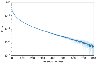
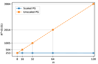
Figure 1: Convergence and robustness of the PG method (2.26).

Appendix A Proofs of technical results

The following lemma establishes the well-posedness of stochastic differential equations, whose coefficients are Lipschitz continuous in state with time-dependent Lipschitz constants. The proof follows essentially the lines of Theorems 3.2.2 and 3.3.1 (Method 2) in [36], and hence is omitted.

Lemma A.1.

Let $T>0$, $(\Omega,\mathcal{F},{\mathbb{F}},\mathbb{P})$ be a filtered probability space satisfying the usual condition, $b:\Omega\times[0,T]\times{\mathbb{R}}^{d}\rightarrow{\mathbb{R}}^{d}$ and ${\sigma}:\Omega\times[0,T]\times{\mathbb{R}}^{d}\rightarrow{\mathbb{R}}^{d\times d}$ be progressively measurable functions such that $b_{\cdot}(\cdot,0)\in L^{1}(\Omega\times[0,T];{\mathbb{R}}^{d})$ and $\sigma_{\cdot}(\cdot,0)\in L^{2}(\Omega\times[0,T];{\mathbb{R}}^{d\times d})$. Assume that there exists $A\in L^{1}(0,T;{\mathbb{R}})$ and $C\in L^{2}(0,T;{\mathbb{R}})$ such that for all $(\omega,t)\in\Omega\times[0,T]$ and $x,x^{\prime}\in{\mathbb{R}}^{d}$, $|b_{t}(\omega,x)-b_{t}(\omega,x^{\prime})|\leq|A_{t}||x-x^{\prime}|$ and $|\sigma_{t}(\omega,x)-\sigma_{t}(\omega,x^{\prime})|\leq|C_{t}||x-x^{\prime}|$. Then for all $\xi_{0}\in L^{2}(\mathcal{F}_{0};{\mathbb{R}}^{d})$, there exists a unique strong solution $X\in\mathcal{S}^{2}(0,T;{\mathbb{R}}^{d})$ to the following equation

$${\mathrm{d}}X_{t}=b_{t}(X_{t})\,{\mathrm{d}}s+\sigma_{t}(X_{t})\,{\mathrm{d}}W_{t},\quad t\in[0,T];\quad X_{0}=\xi_{0}.$$ (A.1)

Proposition A.2.

Suppose (H.11) holds. Then

1. for all $\mathfrak{m}\in\mathcal{A}$, (2.1) admits a unique strong solution $X^{\mathfrak{m}}\in\mathcal{S}^{2}(0,T;{\mathbb{R}}^{d})$.

2. for all $\nu^{\theta}\in\mathcal{V}$, (2.8) admits a unique strong solution $X^{\theta}\in\mathcal{S}^{2}(0,T;{\mathbb{R}}^{d})$.

Proof.

Let $E=[0,T]\times{\mathbb{R}}^{k}$. We verify that the coefficients of (2.1) and (2.8) satisfy the conditions of Lemma A.1.

To prove Item 1, let $\mathfrak{m}\in\mathcal{A}$ be given, and define $\Phi^{\mathfrak{m}}:\Omega\times[0,T]\times{\mathbb{R}}^{d}\rightarrow{\mathbb{R}}^{d}$ and $\Gamma^{\mathfrak{m}}:\Omega\times[0,T]\times{\mathbb{R}}^{d}\rightarrow\overline{{\mathbb{S}}^{d}_{+}}$ such that for all $(\omega,t,x)\in\Omega\times[0,T]\times{\mathbb{R}}^{d}$, $\Phi^{\mathfrak{m}}_{t}(\omega,x)=\Phi_{t}(x,\mathfrak{m}_{t}(\omega))$ and $\Gamma^{\mathfrak{m}}_{t}(\omega,x)=\Gamma_{t}(x,\mathfrak{m}_{t}(\omega))$, with $\Phi$ and $\Gamma$ defined in (2.2). By Fubini’s theorem and Hölder’s inequality,

$${\mathbb{E}}\left[\int_{0}^{T}|\Phi^{\mathfrak{m}}_{t}(\cdot,0)|\right]\,{\mathrm{d}}t \leq\int_{0}^{T}\left({\mathbb{E}}\left[\int_{{\mathbb{R}}^{k}}|a|\,\mathfrak{m}_{t}({\mathrm{d}}a)\right]|B_{t}|\right){\mathrm{d}}t\leq\|B\|_{L^{2}}\left({\mathbb{E}}\left[\int_{E}|a|^{2}\,\mathfrak{m}_{t}({\mathrm{d}}t,{\mathrm{d}}a)\right]\right)^{\frac{1}{2}}<\infty,$$

$${\mathbb{E}}\left[\int_{0}^{T}|\Gamma^{\mathfrak{m}}_{t}(\cdot,0)|^{2}\,{\mathrm{d}}t\right] \leq\widetilde{C}\|D\|_{L^{\infty}}^{2}{\mathbb{E}}\left[\int_{E}|a|^{2}\,\mathfrak{m}_{t}({\mathrm{d}}t,{\mathrm{d}}a)\right]<\infty.$$

For all $(\omega,t)\in\Omega\times[0,T]$, using $\mathfrak{m}_{t}(\omega)\in\mathcal{P}({\mathbb{R}}^{k})$, $|\Phi^{\mathfrak{m}}_{t}(\omega,x)-\Phi^{\mathfrak{m}}_{t}(\omega,x^{\prime})|\leq|A_{t}||x-x^{\prime}|$ for all $x,x^{\prime}\in{\mathbb{R}}^{d}$. To prove the Lipschitz continuity of $\Gamma^{\mathfrak{m}}$, observe that for all $(t,x,m)\in[0,T]\times{\mathbb{R}}^{d}\times\mathcal{P}_{2}({\mathbb{R}}^{k})$, $\Gamma_{t}(x,m)=(M_{m,t}(x)M_{m,t}(x)^{\top}+N_{m,t}N_{m,t}^{\top})^{1/2}$, where $M_{m,t}(x)\coloneqq C_{t}x+D_{t}\int_{{\mathbb{R}}^{k}}a\,m({\mathrm{d}}a)$ and $N_{m,t}\coloneqq D_{t}\left(\int_{{\mathbb{R}}^{k}}aa^{\top}\,m({\mathrm{d}}a)\right)^{1/2}$. This implies that

$$\begin{pmatrix}\Gamma_{t}(x,m)&0_{d\times d}\\ 0_{d\times d}&0_{d\times d}\end{pmatrix}=\begin{pmatrix}M_{m,t}(x)M_{m,t}(x)^{\top}+N_{m,t}N_{m,t}^{\top}&0_{d\times d}\\ 0_{d\times d}&0_{d\times d}\end{pmatrix}^{\frac{1}{2}}=\left|\begin{pmatrix}M_{m,t}(x)&N_{m,t}\\ 0_{d\times 1}&0_{d\times 1}\end{pmatrix}\right|_{\rm mat},$$

where $0_{m\times n}$ is $m\times n$ zero matrix, and $|\cdot|_{\rm mat}$ is the matrix absolute value defined by $|M|_{\rm mat}=(MM^{\top})^{1/2}$ for any matrix $M$. Then, for all $(t,m)\in[0,T]\times\mathcal{P}_{2}({\mathbb{R}}^{k})$ and $x,x^{\prime}\in{\mathbb{R}}^{d}$,

$$\begin{split}&|\Gamma_{t}(x,m)-\Gamma_{t}(x^{\prime},m)|\\ &\quad=\left|\begin{pmatrix}\Gamma_{t}(x,m)-\Gamma_{t}(x^{\prime},m)&0_{d\times d}\\ 0_{d\times d}&0_{d\times d}\end{pmatrix}\right|=\left|\begin{pmatrix}\Gamma_{t}(x,m)&0_{d\times d}\\ 0_{d\times d}&0_{d\times d}\end{pmatrix}-\begin{pmatrix}\Gamma_{t}(x^{\prime},m)&0_{d\times d}\\ 0_{d\times d}&0_{d\times d}\end{pmatrix}\right|\\ &\quad=\left|\left|\begin{pmatrix}M_{m,t}(x)&N_{m,t}\\ 0_{d\times 1}&0_{d\times 1}\end{pmatrix}\right|_{\rm mat}-\left|\begin{pmatrix}M_{m,t}(x^{\prime})&N_{m,t}\\ 0_{d\times 1}&0_{d\times 1}\end{pmatrix}\right|_{\rm mat}\right|\\ &\quad\leq\sqrt{2}\left|\begin{pmatrix}M_{m,t}(x)&N_{m,t}\\ 0_{d\times 1}&0_{d\times 1}\end{pmatrix}-\begin{pmatrix}M_{m,t}(x^{\prime})&N_{m,t}\\ 0_{d\times 1}&0_{d\times 1}\end{pmatrix}\right|=\sqrt{2}|M_{m,t}(x)-M_{m,t}(x^{\prime})|,\end{split}$$ (A.2)

where the last inequality used the Lipschitz continuity of the matrix absolute value $|\cdot|_{\rm mat}$ (see [1]). Therefore, by the definition of $M_{m,t}(x)$, for all $(\omega,t)\in\Omega\times[0,T]$ and $x,x^{\prime}\in{\mathbb{R}}^{d}$,

$$|\Gamma^{\mathfrak{m}}_{t}(\omega,x)-\Gamma^{\mathfrak{m}}_{t}(\omega,x^{\prime})|\leq\sqrt{2}|M_{\mathfrak{m}_{t}(\omega),t}(x)-M_{\mathfrak{m}_{t}(\omega),t}(x^{\prime})|\leq\sqrt{2}|C_{t}||x-x^{\prime}|.$$

As $A\in L^{1}(0,T;{\mathbb{R}}^{d\times d})$ and $C\in L^{2}(0,T;{\mathbb{R}}^{d\times d})$, the coefficients of (2.1) satisfy the conditions of Lemma A.1, which subsequently implies the well-posedness of (2.1).

To prove Item 2, let $\nu^{\theta}\in\mathcal{V}$ be given, and define $\Phi^{\theta}:[0,T]\times{\mathbb{R}}^{d}\rightarrow{\mathbb{R}}^{d}$ and $\Gamma^{\theta}:[0,T]\times{\mathbb{R}}^{d}\rightarrow\overline{{\mathbb{S}}^{d}_{+}}$ such that for all $(t,x)\in[0,T]\times{\mathbb{R}}^{d}$, $\Phi^{\theta}_{t}(x)=\Phi_{t}(x,\nu^{\theta}_{t}(x))$ and $\Gamma^{\theta}_{t}(x)=\Gamma_{t}(x,\nu^{\theta}_{t}(x))$, with $\Phi$ and $\Gamma$ defined in (2.2). Then by Lemma 3.1, $\Phi^{\theta}_{\cdot}(0)=0$ and $\Gamma^{\theta}_{\cdot}(0)=DV_{\cdot}^{\frac{1}{2}}\in L^{2}(0,T;{\mathbb{R}}^{d\times d})$. Moreover, for all $(t,x)\in[0,T]\times{\mathbb{R}}^{d}$, $|\Phi^{\theta}_{t}(x)-\Phi^{\theta}_{t}(x^{\prime})|\leq(|A_{t}|+|B_{t}K_{t}|)|x-x^{\prime}|$ and by (A.2), $|\Gamma^{\theta}_{t}(x)-\Gamma^{\theta}_{t}(x^{\prime})|\leq(|C_{t}|+|D_{t}K_{t}|)|x-x^{\prime}|$. By (H.11) and $K\in L^{2}(0,T;{\mathbb{R}}^{d\times k})$, $|A|+|BK|\in L^{1}(0,T;{\mathbb{R}})$ and $|C|+|DK|\in L^{2}(0,T;{\mathbb{R}})$. This proves that the coefficients of (2.8) satisfy the conditions of Lemma A.1, and hence the well-posedness of (2.8). ∎

Proof of Proposition 2.4.

For each $\varepsilon>0$, let $X^{\varepsilon}=X^{K^{\varepsilon}}$ be such that $X^{\varepsilon}_{t}=\exp(-\int_{0}^{t}(1+\varepsilon-s)^{-1}\,{\mathrm{d}}s)=\frac{1+\varepsilon-t}{1+\varepsilon}$ for all $t\in[0,1]$. Thus for all $\varepsilon>0$, $\mathcal{C}(K^{\varepsilon})=\frac{1}{(1+\varepsilon)^{2}}$ but $\|K^{\varepsilon}\|_{L^{1}}=\log\left(\frac{1+\varepsilon}{\varepsilon}\right)$.

Now let $\tilde{K}^{\varepsilon}=0.5K^{\varepsilon}$, and $\tilde{X}^{\varepsilon}$ be such that $\tilde{X}^{\varepsilon}_{t}=\exp(-0.5\int_{0}^{t}(1+\varepsilon-s)^{-1}\,{\mathrm{d}}s)=\sqrt{\frac{1+\varepsilon-t}{1+\varepsilon}}$ for all $t\in[0,1]$. Thus for all $\varepsilon>0$,

$$\mathcal{C}(\tilde{K}^{\varepsilon})=0.5^{2}\int_{0}^{1}(K^{\varepsilon}_{t}\tilde{X}^{\varepsilon}_{t})^{2}\,{\mathrm{d}}t=\frac{0.25}{1+\varepsilon}\int_{0}^{1}(1+\varepsilon-t)^{-1}\,{\mathrm{d}}t=\frac{0.25}{1+\varepsilon}\log\left(\frac{1+\varepsilon}{\varepsilon}\right)>0.$$

Hence $\mathcal{C}(\tilde{K}^{\varepsilon})>\mathcal{C}(\bm{0})$ and $\lim_{\varepsilon\rightarrow 0}\frac{\mathcal{C}(\tilde{K}^{\varepsilon})}{\mathcal{C}({K})}=\lim_{\varepsilon\rightarrow 0}0.25(1+\varepsilon)\log\left(\frac{1+\varepsilon}{\varepsilon}\right)=\infty$. ∎

Appendix B Experiment details

This section presents additional details for the numerical experiments in Section 4.

Optimal cost.

Let $P^{\star}\in C([0,T];{\mathbb{R}})$ solve the following Riccati equation: for all $t\in[0,T]$,

$$\begin{split}\left(\tfrac{{\mathrm{d}}P}{{\mathrm{d}}t}\right)_{t}&-B_{t}\left(P_{t}\textstyle\sum_{j=1}^{3}(D^{(j)})^{\top}D^{(j)}+\rho\bar{V}^{-1}\right)^{-1}B^{\top}_{t}P^{2}_{t}=0;\quad P_{T}=\tfrac{\mu}{2}.\end{split}$$ (B.1)

Then the optimal policy of (4.1)-(4.2) satisfies $\nu^{\star}_{t}(x)=\mathcal{N}(K^{\star}_{t}x,V_{t}^{\star})$ for all $(t,x)\in[0,T]\times{\mathbb{R}}$, where

$$\begin{split}K^{\star}_{t}&=-\left(P_{t}^{\star}\textstyle\sum_{j=1}^{3}(D^{(j)})^{\top}D^{(j)}+\rho\bar{V}^{-1}\right)^{-1}B^{\top}_{t}P_{t}^{\star},\quad V^{\star}_{t}=\rho\left(P_{t}^{\star}\textstyle\sum_{j=1}^{3}(D^{(j)})^{\top}D^{(j)}+\rho\bar{V}^{-1}\right)^{-1}.\end{split}$$

Moreover, let $\varphi^{\star}\in C([0,T];{\mathbb{R}})$ satisfy for all $t\in[0,T]$,

$$(\tfrac{{\mathrm{d}}}{{\mathrm{d}}t}{\varphi})_{t}+ \tfrac{1}{2}\textnormal{tr}\left(\left(P^{\star}_{t}\textstyle\sum_{j=1}^{3}(D^{(j)})^{\top}D^{(j)}+\rho\bar{V}^{-1}\right)V^{\star}_{t}\right)+\tfrac{\rho}{2}\left(-3+\ln\left(\tfrac{\det(\bar{V})}{\det(V_{t})}\right)\right)=0;\quad\varphi_{T}=0,$$ (B.2)

Then the optimal cost of (4.1)-(4.2) is given by $\mathcal{C}^{\star}=\frac{1}{2}{\mathbb{E}}[\xi_{0}^{\top}\xi_{0}]P^{\star}_{0}+\varphi^{\star}_{0}$.

Implementation details.

The numerical experiments are coded by using Tensorflow. To examine the linear convergence, the scheme (2.26) is implemented on the uniform time grid $\pi_{c}$ with mesh size $\Delta t=1/128$. Indeed, let $K^{0}\equiv(1/3,1/3,1/3)$ and $V^{0}\equiv 0.1D^{\top}D$ be the initial guess. For each $n\in{\mathbb{N}}_{0}$, given $\theta^{n}=(K^{n}_{i},V^{n}_{i})_{i=0}^{127}$, consider the Euler–Maruyama discretisation of (4.3): $X_{0}=\xi_{0}$ and for all $i=0,\ldots,127$,

$$\begin{split}X_{i+1}=X_{i}+B_{i\Delta t}\left(K^{n}_{i}X_{i}+(V^{n}_{i})^{\frac{1}{2}}\zeta_{i}\right)\Delta t+\sum_{j=1}^{3}D^{(j)}\left(K^{n}_{i}X_{i}+(V^{n}_{i})^{\frac{1}{2}}\zeta_{i}\right)\Delta W^{(j)}_{i},\end{split}$$ (B.3)

where $(\Delta W^{(j)}_{i})_{i=0,\ldots,127,j=1,\ldots 3}$ are independent normal random variables with mean zero and variance $1/128$, and $(\zeta_{i})_{i=0}^{127}$ are independent standard normal random vectors in ${\mathbb{R}}^{3}$. We simulate $N_{\rm MC}=10^{5}$ independent trajectories of (B.3) and approximate $\mathcal{C}(\theta^{n})$ as follows (cf. (3.3)):

$$\begin{split}\widehat{\mathcal{C}}(\theta^{n})\coloneqq&\frac{1}{N_{\rm MC}}\sum_{l=1}^{N_{\rm MC}}\frac{1}{2}\Bigg{(}\mu X_{128,l}^{2}+\rho\sum_{i=0}^{127}\Big{(}(K^{n}_{i})^{\top}\bar{V}^{-1}K^{n}_{i}X_{i,l}^{2}+\textnormal{tr}(\bar{V}^{-1}V^{n}_{i})-3+\ln\left(\tfrac{\det(\bar{V})}{\det(V^{n}_{i})}\right)\Big{)}\Delta t\Bigg{)},\end{split}$$

where $(X_{i,l})_{i=0}^{128}$, $l=1,\ldots,N_{\rm MC}$, represents the $l$-th trajectory of (B.3). The required gradients $(\widehat{\nabla_{K^{n}_{i}}\mathcal{C}},\widehat{\nabla_{V^{n}_{i}}\mathcal{C}})_{i=1}^{127}$ are computed using automatic differentiation along these paths, and for each $i=0,\ldots,127$, the state covariance $\Sigma^{\theta^{n}}_{i\Delta t}$ is estimated by $\widehat{\Sigma}^{n}_{i}\coloneqq\frac{1}{N_{\rm MC}}\sum_{l=1}^{N_{\rm MC}}X^{2}_{i,l}$. The policy is then updated as follows (cf. (2.26)): for all $i=0,\cdots,127$,

$$K_{i}^{n+1}=K_{i}^{n}-\frac{\tau}{\Delta t\widehat{\Sigma}^{n}_{i}}\widehat{\nabla_{K^{n}_{i}}\mathcal{C}},\quad V_{i}^{n+1}=V_{i}^{n}-\frac{\tau}{\Delta t}\left(\widehat{\nabla_{V^{n}_{i}}\mathcal{C}}\,V_{i}^{n}+V_{i}^{n}\,\widehat{\nabla_{V^{n}_{i}}\mathcal{C}}\right).$$

The optimal cost of (4.1)-(4.2) is computed by solving (B.1) and (B.2) with the explicit Euler scheme on $\pi_{c}$, which leads to the value $\mathcal{C}^{\star}=0.0402$.

To examine the robustness of (2.26) in time discretisation, a family of coarser time grids $\pi_{m}=\{i\frac{1}{m}\}_{i=0}^{m}\subset\pi_{c}$, $m\in\{8,16,32,64,128\}$, have been introduced. The PG scheme only updates policy parameters at the grid points of these coarser grids. However, to mimic a continuous-time environment, the performance of each policy iterate is still evaluated by simulating (B.3) on the fine grid $\pi_{c}$ (with mesh size $\Delta t=1/128$). In particular, let $(K^{0},V^{0})$ be given as above. For each $m\in\{8,16,32,64,128\}$ and $n\in{\mathbb{N}}_{0}$, given $\theta^{n}=(K^{n}_{j},V^{n}_{j})_{j=0}^{m-1}$, consider the following Euler-Maruyama discretisation of (4.3): $X_{0}=\xi_{0}$ and for all $j=0,\ldots,m-1$, and all $i=0,\ldots,127$ such that $\frac{j}{m}\leq i\Delta t<\frac{j+1}{m}$,

$$\begin{split}\quad X_{i+1}=X_{i}+B_{i\Delta t}\left(K^{n}_{j}X_{i}+(V^{n}_{j})^{\frac{1}{2}}\zeta_{i}\right)\Delta t+\sum_{j=1}^{3}D^{(j)}\left(K^{n}_{j}X_{i}+(V^{n}_{j})^{\frac{1}{2}}\zeta_{i}\right)\Delta W^{(j)}_{i},\end{split}$$ (B.4)

where $(\Delta W^{(j)}_{i})_{i=0,\ldots,127,j=1,\ldots 3}$ and $(\zeta_{i})_{i=0}^{127}$ are independent random variables as in (B.3). We shall sample $10^{5}$ independent trajectories of (B.4), and use them to approximate the gradients in $(K^{n}_{j},V^{n}_{j})_{j=0}^{m-1}$ and the state covariance $(\Sigma^{\theta^{n}}_{j/m})_{j=0}^{m-1}$ with similar methods as above. The scaled PG method (2.26) then updates the parameters by: for all $j=0,\ldots,m-1$,

$$K_{j}^{n+1}=K_{j}^{n}-\frac{m\tau}{\widehat{\Sigma}^{n}_{j}}\widehat{\nabla_{K^{n}_{j}}\mathcal{C}},\quad V_{j}^{n+1}=V_{j}^{n}-{m\tau}\left(\widehat{\nabla_{V^{n}_{j}}\mathcal{C}}\,V_{j}^{n}+V_{j}^{n}\,\widehat{\nabla_{V^{n}_{j}}\mathcal{C}}\right),\quad\textnormal{with $\tau=0.01$},$$ (B.5)

while the unscaled PG method updates the parameters by: for all $j=0,\ldots,m-1$,

$$K_{j}^{n+1}=K_{j}^{n}-\frac{\tau}{\widehat{\Sigma}^{n}_{j}}\widehat{\nabla_{K^{n}_{j}}\mathcal{C}},\quad V_{j}^{n+1}=V_{j}^{n}-{\tau}\left(\widehat{\nabla_{V^{n}_{j}}\mathcal{C}}\,V_{j}^{n}+V_{j}^{n}\,\widehat{\nabla_{V^{n}_{j}}\mathcal{C}}\right),\quad\textnormal{with $\tau=0.08$}.$$ (B.6)

Let $(\theta^{\pi_{m},n})_{n\in{\mathbb{N}}_{0}}$ be the policy iterate generated by (B.5), define $N^{\pi_{m}}(0.01)$ by

$$N^{\pi_{m}}(0.01)\coloneqq\min\left\{n\in{\mathbb{N}}_{0}\,|\,\widehat{\mathcal{C}}(\theta^{\pi_{m},n})-\mathcal{C}^{\star}_{\pi_{m}})<0.01\right\},$$

where $\mathcal{C}^{\star}_{\pi_{m}}\coloneqq\frac{1}{50}\sum_{n=951}^{1000}\widehat{\mathcal{C}}(\theta^{\pi_{m},n})$ approximates the optimal cost among all piecewise constant polices on $\pi_{m}$. The quantity $N^{\pi_{m}}(0.01)$ is defined similarly for the iterates generated by (B.6).

References

• [1] H. Araki and S. Yamagami, An inequality for Hilbert-Schmidt norm, Communications in Mathematical Physics, 81 (1981), pp. 89–96.
• [2] A. S. Berahas, L. Cao, K. Choromanski, and K. Scheinberg, A theoretical and empirical comparison of gradient approximations in derivative-free optimization, Foundations of Computational Mathematics, 22 (2022), pp. 507–560.
• [3] J. Bu, A. Mesbahi, and M. Mesbahi, Policy gradient-based algorithms for continuous-time linear quadratic control, arXiv preprint arXiv:2006.09178, (2020).
• [4] R. Carmona, Lectures on BSDEs, stochastic control, and stochastic differential games with financial applications, SIAM, 2016.
• [5] A. Cartea, S. Jaimungal, and J. Ricci, Algorithmic trading, stochastic control, and mutually exciting processes, SIAM Review, 60 (2018), pp. 673–703.
• [6] M. Fazel, R. Ge, S. Kakade, and M. Mesbahi, Global convergence of policy gradient methods for the linear quadratic regulator, in International Conference on Machine Learning, PMLR, 2018, pp. 1467–1476.
• [7] D. Firoozi and S. Jaimungal, Exploratory LQG mean field games with entropy regularization, Automatica, 139 (2022), p. 110177.
• [8] M. Geist, B. Scherrer, and O. Pietquin, A theory of regularized Markov decision processes, in International Conference on Machine Learning, PMLR, 2019, pp. 2160–2169.
• [9] M. Giegrich, C. Reisinger, and Y. Zhang, Convergence of policy gradient methods for finite-horizon stochastic linear-quadratic control problems, arXiv preprint arXiv:2211.00617, (2022).
• [10] P. J. Graber, Linear quadratic mean field type control and mean field games with common noise, with application to production of an exhaustible resource, Applied Mathematics & Optimization, 74 (2016), pp. 459–486.
• [11] B. Gravell, P. M. Esfahani, and T. Summers, Learning optimal controllers for linear systems with multiplicative noise via policy gradient, IEEE Transactions on Automatic Control, 66 (2020), pp. 5283–5298.
• [12] B. Hambly, R. Xu, and H. Yang, Policy gradient methods find the Nash equilibrium in $n$-player general-sum linear-quadratic games, arXiv preprint arXiv:2107.13090, (2021).
• [13] B. M. Hambly, R. Xu, and H. Yang, Policy gradient methods for the noisy linear quadratic regulator over a finite horizon, Available at SSRN, (2020).
• [14] A. Han, B. Mishra, P. K. Jawanpuria, and J. Gao, On Riemannian optimization over positive definite matrices with the Bures-Wasserstein geometry, Advances in Neural Information Processing Systems, 34 (2021), pp. 8940–8953.
• [15] Y. Jia and X. Y. Zhou, Policy gradient and actor-critic learning in continuous time and space: Theory and algorithms, The Journal of Machine Learning Research, 23 (2022), pp. 12603–12652.
• [16]  , q-learning in continuous time., The Journal of Machine Learning Research, 24 (2023), pp. 161–1.
• [17] Z. Jin, J. M. Schmitt, and Z. Wen, On the analysis of model-free methods for the linear quadratic regulator, arXiv preprint arXiv:2007.03861, (2020).
• [18] S. M. Kakade, A natural policy gradient, Advances in neural information processing systems, 14 (2001).
• [19] B. Kerimkulov, J.-M. Leahy, D. Šiška, and Ł. Szpruch, Convergence of policy gradient for entropy regularized MDPs with neural network approximation in the mean-field regime, arXiv preprint arXiv:2201.07296, (2022).
• [20] V. Konda and J. Tsitsiklis, Actor-critic algorithms, Advances in neural information processing systems, 12 (1999).
• [21] J. Mei, C. Xiao, C. Szepesvari, and D. Schuurmans, On the global convergence rates of softmax policy gradient methods, in International Conference on Machine Learning, PMLR, 2020, pp. 6820–6829.
• [22] R. Munos, Policy gradient in continuous time, Journal of Machine Learning Research, 7 (2006), pp. 771–791.
• [23] S. Park, J. Kim, and G. Kim, Time discretization-invariant safe action repetition for policy gradient methods, Advances in Neural Information Processing Systems, 34 (2021), pp. 267–279.
• [24] C. Reisinger, W. Stockinger, and Y. Zhang, Linear convergence of a policy gradient method for finite horizon continuous time stochastic control problems, arXiv preprint arXiv:2203.11758, (2022).
• [25] J. Schulman, S. Levine, P. Abbeel, M. Jordan, and P. Moritz, Trust region policy optimization, in International conference on machine learning, PMLR, 2015, pp. 1889–1897.
• [26] J. Schulman, F. Wolski, P. Dhariwal, A. Radford, and O. Klimov, Proximal policy optimization algorithms, arXiv preprint arXiv:1707.06347, (2017).
• [27] D. Šiška and Ł. Szpruch, Gradient flows for regularized stochastic control problems, arXiv preprint arXiv:2006.05956, (2020).
• [28] J. Sun, X. Li, and J. Yong, Open-loop and closed-loop solvabilities for stochastic linear quadratic optimal control problems, SIAM Journal on Control and Optimization, 54 (2016), pp. 2274–2308.
• [29] R. S. Sutton, D. McAllester, S. Singh, and Y. Mansour, Policy gradient methods for reinforcement learning with function approximation, Advances in neural information processing systems, 12 (1999).
• [30] L. Szpruch, T. Treetanthiploet, and Y. Zhang, Optimal scheduling of entropy regulariser for continuous-time linear-quadratic reinforcement learning, arXiv preprint arXiv:2208.04466, (2022).
• [31] C. Tallec, L. Blier, and Y. Ollivier, Making Deep Q-learning methods robust to time discretization, arXiv preprint arXiv:1901.09732, (2019).
• [32] H. Wang, T. Zariphopoulou, and X. Y. Zhou, Reinforcement learning in continuous time and space: A stochastic control approach, Journal of Machine Learning Research, 21 (2020), pp. 1–34.
• [33] H. Wang and X. Y. Zhou, Continuous-time mean–variance portfolio selection: A reinforcement learning framework, Mathematical Finance, 30 (2020), pp. 1273–1308.
• [34] W. Wang, J. Han, Z. Yang, and Z. Wang, Global convergence of policy gradient for linear-quadratic mean-field control/game in continuous time, in International Conference on Machine Learning, PMLR, 2021, pp. 10772–10782.
• [35] J. Yong and X. Y. Zhou, Stochastic Controls: Hamiltonian Systems and HJB Equations, vol. 43, Springer Science & Business Media, 1999.
• [36] J. Zhang, Backward Stochastic Differential Equations, Springer, 2017.
• [37] K. Zhang, B. Hu, and T. Basar, Policy optimization for $\mathcal{H}_{2}$ linear control with $\mathcal{H}_{\infty}$ robustness guarantee: Implicit regularization and global convergence, SIAM Journal on Control and Optimization, 59 (2021), pp. 4081–4109.
• [38] K. Zhang, X. Zhang, B. Hu, and T. Basar, Derivative-free policy optimization for linear risk-sensitive and robust control design: Implicit regularization and sample complexity, Advances in Neural Information Processing Systems, 34 (2021), pp. 2949–2964.
• [39] X. Y. Zhou and D. Li, Continuous-time mean-variance portfolio selection: A stochastic LQ framework, Applied Mathematics and Optimization, 42 (2000), pp. 19–33.