Rawgment: Noise-Accounted RAW Augmentation Enables Recognition in a Wide Variety of Environments

Abstract

Image recognition models that work in challenging environments (e.g., extremely dark, blurry, or high dynamic range conditions) must be useful. However, creating training datasets for such environments is expensive and hard due to the difficulties of data collection and annotation. It is desirable if we could get a robust model without the need for hard-to-obtain datasets. One simple approach is to apply data augmentation such as color jitter and blur to standard RGB (sRGB) images in simple scenes. Unfortunately, this approach struggles to yield realistic images in terms of pixel intensity and noise distribution due to not considering the non-linearity of Image Signal Processors (ISPs) and noise characteristics of image sensors. Instead, we propose a noise-accounted RAW image augmentation method. In essence, color jitter and blur augmentation are applied to a RAW image before applying non-linear ISP, resulting in realistic intensity. Furthermore, we introduce a noise amount alignment method that calibrates the domain gap in the noise property caused by the augmentation. We show that our proposed noise-accounted RAW augmentation method doubles the image recognition accuracy in challenging environments only with simple training data.

1 Introduction

Although image recognition has been actively studied, its performance in challenging environments still needs improvement [16]. Sensitive applications such as mobility sensing and head-mounted wearables need to be robust to various kinds of difficulties, including low light, high dynamic range (HDR) illuminance, motion blur, and camera shake. One possible solution is to use image enhancement and restoration methods. A lot of DNN-based low-light image enhancement [30, 55, 21, 47, 13, 31], denoising [54, 33, 44], and deblurring [53, 49, 44] methods are proposed to improve the pre-captured sRGB image quality. While they are useful for improving pre-captured image quality, a recent work [16] shows that using them as preprocessing for image recognition models has limited accuracy gains since they already lost some information, and restoring the lost information is difficult.

Figure 1: The concept of the proposed noise-accounted RAW augmentation. Conventional augmentation (a) is applied to the output of an ISP; due to the nonlinear operations in the ISP, it produces images that cannot be captured at any ambient light intensities. Instead, ours (b) applies augmentation before an ISP. It generates realistic pixel intensity distribution that can be captured when the light intensity is different. Moreover, the noise amount is also corrected to minimize the domain gap between real and augmented ones.

Another possible solution is to prepare a dataset for difficult environments [34, 3]. However, these datasets only cover one or a few difficulties, and creating datasets in various environments is too expensive. Especially, manual annotation of challenging scenes is difficult and time-consuming. For example, we can see almost nothing in usual sRGB images under extremely low-light environments due to heavy noise. In addition, some regions in HDR scenes suffer from halation or blocked-up shadows because the 8-bit range of usual sRGB images cannot fully preserve the real world, which is 0.000001 $[cd/m^{2}]$ under starlight and 1.6 billion $[cd/m^{2}]$ under direct sunlight [38]. Heavy motion blur and camera shake also make annotation difficult. Some works capture paired short-exposure and long-exposure images, and the clean long-exposure images are used for annotation or ground truth [16, 17, 18, 20]. The limitation is that the target scene needs to be motionless if the pairs are taken sequentially with one camera [16], and positional calibration is required if the pairs are taken with synchronized cameras [17, 18]. Some works use a beam splitter to capture challenging images and their references without calibration [46, 20]. However, they are difficult to apply in dark scenes. Moreover, HDR images cannot be taken in the same way because some regions become overexposed or underexposed in both cameras.

To this end, we aim to train image recognition models that work in various environments only using a training dataset in simple environments like bright, low dynamic range, and blurless. In this case, image augmentation or domain adaptation is important to overcome the domain gap between easy training data and difficult test data. However, we believe usual augmentations on sRGB space are ineffective because it does not take into account the nonlinear mapping of ISPs. In particular, tone mapping significantly changes the RAW image values, which are roughly proportional to physical brightness [45]. Contrast, brightness, and hue augmentation on sRGB space result in unrealistic images that cannot be captured under any ambient light intensity as shown in Fig. 1(a). In contrast, we propose augmentation on RAW images. In other words, augmentation is applied before ISPs to diminish the domain shift as shown in Fig. 1(b).

Oher possible sources of the domain gap are differences in noise amount and noise distribution. To tackle these problems, we propose a method to align both light intensity and noise domains. Recent works show that adding physics-based realistic noise improves the performance of DNN-based denoisers [45, 48, 2, 51] and dark image recognition [16, 4]. Although their proposed sensor noise modelings are accurate, they assume that the original bright images are noise free. In contrast, we propose to modify the noise amount after contrast, brightness, and hue conversion considering the noise amount in the original images. It enables a more accurate alignment of the noise domain. Even bright images may have dark areas due to shadows or object colors, and their prior noise cannot be ignored. Another merit of our method is that it is possible to take dark images that already contain a lot of noise as input. In addition to noise alignment after color jitter augmentation, we show the importance of noise alignment after blur augmentation, which is proposed for the first time in this paper.

Our contributions are as follows:

• It is the first work to emphasize the importance of augmentation before ISP for image recognition to the best of our knowledge.

• Noise amount alignment method is proposed to reduce the noise domain gap after RAW image augmentation. In contrast to previous works, our proposed method takes into account prior noise in the input image. It enables more accurate alignment and use of any strength of augmentation and even already noisy input.

• We show qualitative analysis for the validity of our sensor noise modeling and corresponding noise-accounted augmentation. We prove that our proposed noise-accounted RAW augmentation has the edge over the previous methods.

2 Related Works

2.1 Recognition in Difficult Environment

Many works have tackled image recognition in difficult environments. For low-light environments, several works improve the accuracy by replacing a traditional ISP with a powerful DNN-based ISP to create clean images for downstream image recognition models [6, 34, 26]. Even though these methods are promising because there is no information loss, the computational cost is the problem. Another approach is direct RAW image recognition without ISP [40, 16]. Their image recognition models benefit from the richest information and improve accuracy under low-light environments. However, several works report ISPs, especially tone mapping, are helpful for machine vision [50, 14]. Direct RAW image recognition may works well if the images have a low dynamic range. Another approach is domain adaptation or related methods which support low-light recognition with bright images [39, 16, 4].

For HDR environments, some works propose DNN-based auto-exposure control [43, 36] to improve downstream recognition. Also, multi-frame HDR synthesis methods [7, 1] can be used as a preprocessing, although camera motion makes them challenging. A luminance normalization method is also introduced to improve recognition performance under varying illumination conditions [19].

For blurry environments, deblurring methods are actively studied [49, 52]. These DNN-based methods successfully restore clear images from heavily blurred images.

Differing from the above, we aim to do image recognition under all the above difficulties using simple scene training data with our proposed augmentation method. We do not use domain adaptation methods since these methods are usually used in a setting where the target domain is equal to or smaller than the source domain [11]. On the contrary, in our setting, the distribution of the target domain is much wider than that of the source domain.

2.2 Image Conversion on RAW

Recently, several methods [2, 30, 4] convert bright sRGB images into realistic dark images by the following procedures. First, they invert an ISP pipeline to generate RAW-like images followed by illumination change on the RAW data space with plausible sensor noise. Afterward, degraded sRGB is generated by applying the forward ISP pipeline. This operation avoids the nonlinear mappings in the ISP and simulates short exposures and dark environments. With a similar intention, we propose to apply augmentation before ISPs to train image recognition models.

2.3 Noise Modeling and Noise Amount Alignment

In the electronic imaging sensor community, detailed noise modelings based on electric current and circuit have been studied [42, 8, 24, 12]. They are precise but difficult to be applied to the image-to-image conversion. Thus, in the machine vision community, simplified pixel value-based noise modelings are proposed based on electric noise modelings [45, 48, 2]. Although the noise model of [48] is well designed with a high degree of freedom Tukey lambda distribution [22], we are based on the well-established heteroscedastic Gaussian model [2, 37, 10, 51] because it is still well fitted to real sensor noise and we can consider prior noise in original images which will be explained later.

Recently, adding realistic model-based sensor noise to the ground truth clean images is proved to be helpful to train DNN-based denoiser [45, 51, 48, 2] and low-light object detection models [16, 4]. Although they use highly consistent noise models, they regard original images as noise-free. In contrast, we propose to modify the noise amount after image conversion considering the noise amount of the original images. It enables a more accurate alignment of the noise domain and enables the use of any intensity of augmentation and already noisy images as input.

3 Methodology

In this section, we introduce our noise model, calibration procedure, and proposed noise-accounted RAW augmentation.

3.1 Noise Model

First, we briefly introduce our noise model for later explanation although it is based on the well-established heteroscedastic Gaussian model [2, 37, 10, 51]. The number of photons $u$ hitting the photodiode of each pixel is converted to a voltage with quantum efficiency $\alpha$. Some processing is then performed to read out the voltage, in which noise $n_{d}$ is inevitably mixed. Next, analog gain $g$ is multiplied to amplify the value. Lastly, the voltage is converted to a digital value. We simplify and summarize the noise after analog gain as $n_{r}$. Since it is common to use analog gain which has a better signal-to-noise ratio (SNR), we omit the digital gain term in our noise model. To sum up, the photon-to-RAW pixel value conversion can be formulated as,

$$x=g\left(\alpha u+n_{d}\right)+n_{r}.$$ (1)

We approximate $n_{d}$ and $n_{r}$ as Gaussian noise $\mathcal{N}\left(0,\sigma_{d}^{2}\right)$ $\mathcal{N}\left(0,\sigma_{r}^{2}\right)$ and the number of photons $u$ itself obeys the Poisson distribution $\mathcal{P}\left(\bar{u}\right)$ where $\bar{u}$ is the expected number of photons. If $\bar{u}$ is large enough, we can approximate as $\mathcal{P}\left(\bar{u}\right)\fallingdotseq\mathcal{N}\left(\bar{u},\bar{u}\right)$ [10]. Thus, our noise model is as follows;

$$x\sim g\left(\alpha\mathcal{N}\left(\bar{u},\bar{u}\right)+\mathcal{N}\left(0,\sigma_{d}^{2}\right)\right)+\mathcal{N}\left(0,\sigma_{r}^{2}\right).$$ (2)

We show the validity of the Gaussian approximation of $n_{d}$, $n_{r}$, and $\mathcal{P}\left(\bar{u}\right)$ in the Section 4.3. We don’t follow the further development of the formula in [10] for our purpose.

Gaussian distribution has the following convenient natures;

$$\begin{cases}X\sim\mathcal{N}\left(\mu_{X},\sigma_{X}^{2}\right)\\ Y\sim\mathcal{N}\left(\mu_{Y},\sigma_{Y}^{2}\right)\\ X+Y\sim\mathcal{N}\left(\mu_{X}+\mu_{Y},\sigma_{X}^{2}+\sigma_{Y}^{2}\right)\\ cX\sim\mathcal{N}\left(c\mu_{X},c^{2}\sigma_{X}^{2}\right)\end{cases},$$ (3)

if $X$ and $Y$ are independent, and that’s why we choose the simple Gaussian approximation instead of the recently proposed more expressive noise model [48]. These natures enable the proposed noise-accounted RAW augmentation to account for prior noise in input images. Furthermore, they further simplify our noise model as,

$$x\sim\mathcal{N}\left(g\alpha\bar{u},g^{2}\alpha^{2}\bar{u}+g^{2}\sigma_{d}^{2}+\sigma_{r}^{2}\right).$$ (4)

Because the expected number of photon $\bar{u}$ is inconvenient to use in image-to-image conversion, we replace it with the expected pixel value $\mu_{x}=g\alpha\bar{u}$, and our final noise model is defined as,

$$x\sim\mathcal{N}\left(\mu_{x},\sigma_{x}^{2}=g\alpha\mu_{x}+g^{2}\sigma_{d}^{2}+\sigma_{r}^{2}\right).$$ (5)

3.2 Noise Model Calibration

Figure 2: Our noise model calibration procedures to a target sensor. It just needs to capture burst RAW images and does not need special devices.

Our sensor noise model shown in Eq. (5) has three parameters, $\alpha$, $\sigma_{d}^{2}$, and $\sigma_{r}^{2}$, which have to be calibrated per target sensor. We capture a series of RAW images of a color checker as shown in Fig. 2(a). We then calculate the mean $\mu_{x}$ and variance $\sigma_{x}^{2}$ along the time direction of each pixel position. We calculate them along the time direction instead of the spatial direction as performed in [45] since lens distortion changes the luminance of the same color patch. These operations are performed several times by changing the analog gain and exposure time. Eventually, we get various sets of $\left\{\mu_{x},\sigma_{x}^{2}\right\}$ for each analog gain. Note that we calculate mean and variance without separating RGB channels because there is no significant difference in noise properties.

In Eq. (5), $\mu_{x}$ and $\sigma_{x}^{2}$ have a linear relationship per analog gain $g_{n}$;

$$\sigma_{x}^{2}=a_{g_{n}}\mu_{x}+b_{g_{n}}.$$ (6)

Therefore, we solve linear regression to estimate $a_{g_{n}}$ and $b_{g_{n}}$ per gain like Fig. 2(b). In addition, we use RANSAC [9] to robustly take care of outlier $\left\{\mu_{x},\sigma_{x}^{2}\right\}$ pairs.

Finally, we estimate $\alpha$, $\sigma_{d}^{2}$, and $\sigma_{r}^{2}$ from the following redundant simultaneous equations by least-squares method,

$$\begin{cases}a_{g_{1}}=g_{1}\alpha\\ \>\>\>\vdots\\ a_{g_{n}}=g_{n}\alpha\end{cases},$$ (7)

$$\begin{cases}b_{g_{1}}=g_{1}^{2}\sigma_{d}^{2}+\sigma_{r}^{2}\\ \>\>\>\vdots\\ b_{g_{n}}=g_{n}^{2}\sigma_{d}^{2}+\sigma_{r}^{2}\end{cases}.$$ (8)

The procedure above enables calibration of the sensor noise model without special devices. We later show that our sensor model and the calibration method represent the real sensor noise with enough preciseness.

3.3 Noise-Accounted RAW Augmentation

We propose augmentation before ISP instead of the usual augmentation after ISP to generate realistic images. Furthermore, we improve the reality of the augmented images by considering the sensor noise model. Unlike the previous works [45, 48, 4, 16, 2, 51], ours takes the prior noise amount of input images into account. It generates more realistic noise since even bright images have some extent of noise. Especially, dark parts due to shadow or the color of objects might have a non-negligible amount of noise. Moreover, it allows any brightness of input images different from previous works. Specifically, we introduce how to adjust noise amount after contrast, brightness, hue, and blur augmentation.

3.3.1 Color Jitter Augmentation

Contrast, brightness, and hue augmentation simulate different exposure times, light intensities, and analog gain. Hence, we first assume to multiply the exposure time, light intensity, and analog gain by $p_{e}$, $p_{i}$, and $p_{g}$ respectively. Because $p_{e}$ and $p_{i}$ equally change the number of photon $u$ in the case of our noise model, we rewrite them as $p_{u}=p_{e}p_{i}$. Then, images in the above environment settings $x_{new}$ can be rewritten as,

$$x_{new}\sim\mathcal{N}\left(\begin{split}(p_{g}g)\alpha(p_{u}\bar{u}),\\ (p_{g}g)^{2}\alpha^{2}(p_{u}\bar{u})+(p_{g}g)^{2}\sigma_{d}^{2}+\sigma_{r}^{2}\end{split}\right).$$ (9)

Based on Eq. (3), it can be expanded as

$$x_{new} \sim\mathcal{N}\left((p_{g}p_{u})\alpha g\bar{u},\>(p_{g}p_{u})^{2}(g^{2}\alpha^{2}\bar{u}+g^{2}\sigma_{d}^{2}+\sigma_{r}^{2})\right)$$

$$\>\>\>\;+\mathcal{N}\left(\right.0,\>-(p_{g}p_{u})^{2}(g^{2}\alpha^{2}\bar{u}+g^{2}\sigma_{d}^{2}+\sigma_{r}^{2})$$ (10)

$$\>\>\>\>\;\>\>\;\>\>\>\>\>\>\;\>\>\>\>\>\>\>+(p_{g}g)^{2}\alpha^{2}(p_{u}\bar{u})+(p_{g}g)^{2}\sigma_{d}^{2}+\sigma_{r}^{2}\left.\right).$$

By inserting $\mu_{x}=g\alpha\bar{u}$ and original pixel value, $x_{pre}\sim\mathcal{N}\left(\mu_{x},g\alpha\mu_{x}+g^{2}\sigma_{d}^{2}+\sigma_{r}^{2}\right)$, it can be expressed with a pixel value-based equation as follows;

$$x_{new} \sim p_{u}p_{g}x_{pre}+$$

$$\>\>\>\;\mathcal{N}(0,\>p_{u}(1-p_{u})p_{g}^{2}g\alpha\mu_{x}$$ (11)

$$\>\;\>\>\;\>\>\>\>\>\>\;\>\>+(1-p_{u}^{2})p_{g}^{2}g^{2}\sigma_{d}^{2}+(1-p_{u}^{2}p_{g}^{2})\sigma_{r}^{2}).$$

Because the expected original pixel value $\mu_{x}$ in the Gaussian term is impossible to obtain, we approximate it as $\mu_{x}=x_{pre}$. Based on this equation, we can precisely simulate as if exposure time, light intensity, and analog gain were $p_{e}$, $p_{i}$, and $p_{g}$ times. Then, let’s come back to contrast, brightness, and hue augmentation. When contrast is multiplied by $p_{c}$ and brightness is changed by $p_{b}$, it can be expressed as,

$$x_{new}=p_{c}x_{pre}+p_{b}.$$ (12)

This function is represented as multiplication by $\frac{\left(p_{c}x_{pre}+p_{b}\right)}{x_{pre}}$. Therefore, noise-accounted contrast and brightness augmentation is finally defined as,

$$\begin{cases}random\>p_{c},\>p_{b}\\ random\>p_{u},\>p_{g}\>(where\>p_{u}p_{g}=\frac{\left(p_{c}x_{pre}+p_{b}\right)}{x_{pre}},\>p_{u},p_{g}>0)\\ Eq.(\ref{eq:11})\>(\mu_{x}\leftarrow x_{pre})\end{cases}.$$ (13)

We can also convert hue by changing $p_{c}$ and $p_{b}$ per color filter position in the RAW bayer.

3.3.2 Blur Augmentation

Next, we introduce noise-accounted blur augmentation. Usual blur augmentation makes noise smaller than actual blur because the noise $n_{d}$ and $n_{r}$ are smoothed out although their noise amounts, in reality, are not related to how fast you shake a camera or how fast objects move. Only the photon number-related noise is smoothed out in actual motion blur. The actual blurred pixel is expressed as,

$$x_{new}\sim\mathcal{N}\left(g\alpha\sum_{k}w_{k}\bar{u_{k}},\>g^{2}\alpha^{2}\sum_{k}w_{k}\bar{u_{k}}+g^{2}\sigma_{d}^{2}+\sigma_{r}^{2}\right),$$ (14)

where $\sum_{k}w_{k}=1$ is the blur kernel. With similar equation manipulation from Eq. (9) to Eq. (11) , noise-accounted blur augmentation is

$$x_{new} \sim\mathcal{N}\left(\sum_{k}w_{k}g\alpha\bar{u_{k}},\>\sum_{k}w_{k}^{2}(g^{2}\alpha^{2}\bar{u_{k}}+g^{2}\sigma_{d}^{2}+\sigma_{r}^{2})\right)$$

$$\>\;\>\>+\mathcal{N}(0,\>-\sum_{k}w_{k}^{2}(g^{2}\alpha^{2}\bar{u_{k}}+g^{2}\sigma_{d}^{2}+\sigma_{r}^{2})$$

$$\>\;\>\>\;\>\>\>\>\>\>\;\>\>\;\>\>\>\>+g^{2}\alpha^{2}\sum_{k}w_{k}\bar{u_{k}}+g^{2}\sigma_{d}^{2}+\sigma_{r}^{2})$$ (15)

$$=\sum_{k}w_{k}x_{pre}+\mathcal{N}(0,\>g\alpha\sum_{k}(1-w_{k})w_{k}x_{pre,k}$$

$$\>\;\>\;\>\>\;\>\>\>\>\>\>\;\>\>\;\>\>\>\>\>\>\;\>\>\;\>\>\;\>\>\>\;\>\>\;\>\>+(1-\sum_{k}w_{k}^{2})(g^{2}\sigma_{d}^{2}+\sigma_{r}^{2})).$$

We account for prior noise but not for prior blur amounts because most images in usual datasets are not very blurry. Furthermore, it is difficult to estimate the prior blur amount.

In addition, please note that augmentation to make images clean (make them brighter and deblurred) is inevitably difficult with noise-accounted RAW augmentation. Clipping noise variance in Eq. (11) to zero forcibly enables brightening, but brightening too much causes a mismatch of noise domain.

4 Evaluation

4.1 Dataset

Figure 3: Examples of the introduced dataset. The upper row shows the training dataset collected in simple environments while the lower row shows the challenging test dataset collected in various environments from dark to bright, HDR, and with or without handshake blur.

Although our method can be applied to any computer vision task, we choose a human detection task as a target because of its wide usage. We prepared a RAW image dataset for human detection task captured with an internally developed sensor. As mentioned earlier, our objective is to train image recognition models that work in various environments only using a training dataset in simple environments. So, most training images are taken under normal light conditions with fixed camera positions in several environments. Note that moderately dark and HDR images are also included to some extent in the training dataset. The analog gain is set to 6dB outdoors, 12dB indoors, and 32dB at night in moderate darkness to generate realistic easy images without auto-exposure. Test images, on the other hand, are taken in HDR or extremely dark environments. In addition, about 50% of them are captured with a strong camera shake. Moreover, the analog gain is chosen from 3dB, 6dB, 12dB, and 24dB regardless of the environment. Both datasets are captured with around 1 fps to increase diversity among images.

We manually annotate the human bounding boxes of both training and test data. Because precise annotation of test data on sRGB is impossible due to the noise and blur, we apply an offline ISP to each image and then annotate the bounding boxes. We manually set adequate ISP parameters per image and had to change the parameters several times to grasp the entire image. To avoid annotating large training datasets in this time-consuming way, it is desirable to train the model with a simple dataset. In total, 18,880 images are collected for training and 2,800 for testing. The examples are shown in Fig. 3.

4.2 Implementation Details

We mainly test with TTFNet [28] whose backbone is ResNet18 [15]. The network is trained for 48 epochs from scratch using Adam optimizer [23] and a cosine decay learning rate scheduler with a linear warmup [29] for the first 1,000 iterations whose maximum and minimum learning rates are 1e-3 and 1e-4. As to an ISP, a simple software ISP consisting of only a gamma tone mapping is implemented. In detail, two types of gamma tone mapping are implemented. One is the simplest gamma tone mapping, $y=x^{\frac{1}{\gamma}}\>(0\leq x\leq 1)$. The $\gamma$ is set to 5 after tuning with a rough grid search manner. The other is a gamma tone mapping parameterized with three parameters [35]. Because the grid search for three parameters is time-consuming, we tuned the parameters with backpropagation together with the detector’s weights as performed in [36, 50]. Other ISP functions are not used because they are known to have less impact on image recognition compared with tone mapping [14]. We also prepare an elaborated black-box ISP consisting of many functions in addition to a tone mapping function. The parameters are tuned for human perceptual quality by experts. We only use the elaborated black-box ISP under the conventional training pipeline. In other words, experiments are performed under ISP-augmentation-detection order with the elaborated black-box ISP due to the hardware limitation. If contrast augmentation is used, the hue is also changed with a probability of 50%. In detail, the contrast factor per color channel $p_{c,h=\{R,G,B\}}$ is randomized from the base contrast factor $p_{c,base}$ by (0.8$p_{c,base}$, 1.2$p_{c,base}$) after $p_{c,base}$ is randomly decided. If blur augmentation is used, a random-sized blur kernel with a probability of 50% is used. Random shift and random scale augmentation whose maximum transformations are 10% and 3% of the input size are also applied with a probability of 80% before color jitter augmentation. The input size to the detector is $\left(576,\,352,\,3\right)$. The performance of the detector is evaluated with average precision (AP@0.5:0.95) [25].

4.3 Calibration of the Noise Model

For each analog gain of 6dB, 12dB, and 24dB, two burst sequences are captured with different illumination. Each sequence consists of 100 images. $24\times 24$ Bayer pixels are sampled from each of the 24 color patches to calculate the mean and variance. In total $2\times 24\times 24\times 24$ pairs of mean and variance sets are obtained per analog gain to estimate the noise model. Thanks to the various color filters, exposure values, and color patches, two sequences are enough to ensure diversity. The lines in Fig. 4 show the estimated linear relationship in Eq. (6). The coefficients of determination, $R^{2}$, for these line estimations are 0.9833, 0.9884, 0.9862 for 6, 12, and 24dB respectively. High values of $R^{2}$ indicate that the noise intensity is well modeled with respect to illumination intensity. Also, $R^{2}$ of the Eq. (7) and Eq. (8) are $1.0000$ and $0.9984$. This means the noise intensity is well modeled with respect to the analog gain. Based on the above, our noise model and the calibration method are well suited to the sensor in terms of noise intensity.

Figure 4: Sensor noise model calibration result. The dots in the left graph are the mean and variance pairs for each pixel, and the lines are the estimated linear relationship for each analog gain. Since large numbers of dots are plotted, they seem to be widely spread. On the other hand, the histogram plot per analog gain (right) shows a clear difference between them.

Figure 5: The result of the Shapiro-Wilk [41] test for each expected pixel value. When testing whether the 100 pixel values at each location correspond to a Gaussian distribution, most p-values are larger than 0.05 (a). The right (b) shows the cases where p < 0.05. It indicates the small p-values come from sparsity, not skew.

Next, we check the validity of the shape of the distribution. All noises were assumed to follow a Gaussian distribution. Especially, it is unclear whether the approximation $\mathcal{P}\left(\bar{u}\right)\fallingdotseq\mathcal{N}\left(\bar{u},\bar{u}\right)$ [10] is true. Therefore, the Shapiro-Wilk test [41] is performed. If the p-value of the test is higher than 0.05, it indicates that we cannot reject the null hypothesis that the data are normally distributed with more than a 95% confidence interval. Fig. 5(a) shows that most of them are higher than 0.05, but some results for dark pixels are less than 0.05. However, the distributions of the dark pixels are like Fig. 5(b). It is not very skewed and the sparsity causes the small p-value. Therefore, we conclude that all the noise sources can be regarded as Gaussian noise.

Based on the above, our sensor noise model and the calibration method represent the sensor noise well in terms of both intensity and distribution.

4.4 Statistical Validation of the Noise Alignment

Before confirming the effectiveness of the proposed noise-accounted RAW augmentation to computer vision applications, the statistical validity is evaluated one more time by utilizing the series of color checker images. The evaluation method is as follows. First, the contrast of the sequential images is changed with or without noise consideration. Second, mean and variance pairs along the sequential dimension are computed. Third, the distributions of real and converted pairs are examined. If the real and converted pairs matched well, it means the converted images have the same noise amount as the original real images.

Three different noise alignment methods are compared, i.e., no noise consideration, the usual noise-accounted method that disregards prior noise in the input [16, 4, 45, 48], and our proposed noise alignment method. Fig. 6 shows the comparison result. It indicates that prior noise consideration is unnecessary if pixels are darkened considerably. However, a small contrast factor caused a noise domain gap even if the input is bright like Fig. 6 (right). In contrast, our noise-accounted conversion always converted images with realistic noise. It implies that our proposed method is suited for various strengths of augmentation. If prior noise is not accounted for, the inputs always have to be darkened considerably and already dark images are difficult to use.

Figure 6: The statistical validation of the noise alignment. The green dots represent real image data, and the others are converted from it. The conversions are ×0.1 and ×0.5 contrast conversion with several methods. The (a) is a dark-to-extreme-dark conversion, and the (b) is a bright-to-dark conversion.

4.5 Augmentation Parameters Tuning

The optimal augmentation parameters should be different between augmentation before and after ISP. To make a fair comparison, we roughly tune both of the augmentation parameters. The strategy is as follows. First, we search the appropriate range of contrast factor $p_{c}$ and brightness perturbation $p_{b}$ successively. To be robust to any illumination of inputs, we re-parameterize $p_{b}$ as $p_{b}=\hat{p_{b}}min(x)$ and randomize the $\hat{p_{b}}$ instead of $p_{b}$. Lastly, we search for the appropriate max blur distance $p_{d}$. In these experiments, we do not account for sensor noise. We use the elaborated black-box ISP for the augmentation after ISP setting and the simplest gamma function for the augmentation before ISP setting.

The results are shown in Table 1. The best parameter settings are used in the next section.

Table 1: The augmentation hyperparameter tuning for a fair comparison between before and after ISP augmentation. The range of contrast, brightness, and blur distance are tuned one by one, taking over the previous best parameters.

		augmentation after ISP (tuned for the black-box ISP)					augmentation before ISP (tuned for the simplest ISP)
contrast	range	0.2-1	0.1-1	0.2-5	0.1-10	0.05-20	0.1-1	0.02-1	0.01-1	0.005-1	0.01-1.1
	AP@0.5:0.95 [%]	41.9	41.8	43.2	45.1	44.5	36.9	39.8	40.4	35.8	38.9
brightness	range	0-0	-0.1-0.1	-0.2-0.2	-0.5-0.5	-0.7-0.7	0-0	-0.1-0.1	-0.2-0.2	-0.5-0.5	-0.7-0.7
	AP@0.5:0.95 [%]	45.1	44.5	44.5	45.2	44.7	40.4	40.9	39.9	39.4	39.4
blur distance	range	0-0	0-3	0-5	0-9	0-13	0-0	0-3	0-5	0-9	0-13
	AP@0.5:0.95 [%]	45.2	46.8	45.7	45.9	37.9	40.9	39.8	39.6	40.6	43.3

4.6 Evaluation of the Noise-Accounted RAW Augmentation

In this section, the proposed noise-accounted RAW augmentation is evaluated on training image recognition models. First, as Table 2 shows, augmentation before ISP drastically improves the accuracy with the simplest ISP. It suggests the realistic pixel intensity distribution achieved by augmentation before ISP is the key to improving the accuracy in wide environments. In the color jitter augmentation only setting, the accuracy is improved from the general noise alignment method [10, 32, 16, 4, 27, 48, 37, 51, 2] by considering prior noise. In the color jitter and blur augmentation setting, noise-accounted color jitter augmentation plus normal blur augmentation does not improve much from no noise-accounted settings. Instead, noise alignment in both color jitter and blur augmentation improves the accuracy. It indicates that random noise is not effective and realistic noise is important. Comparing the accuracy under the same simplest gamma tone mapping setting, our proposed noise-accounted RAW augmentation doubles the accuracy of conventional augmentation after ISP. Furthermore, when parameterized gamma tone mapping is used as our simple ISP, the accuracy is even superior to the elaborated black-box ISP consisting of many functions in addition to a tone mapping function. As the visualization results in the supplementary material show, the elaborated black-box ISP outputs more perceivable images. It suggests that minimizing the domain gap caused by augmentation is more important than the superiority of the ISP. We might improve the accuracy more by an elaborated ISP and the proposed augmentation.

Table 2: Evaluation of the noise-accounted RAW augmentation. The color augmentation contains default hue augmentation plus tuned contrast and brightness augmentation. The w/o prior means the prior input noise is disregarded like many of the previous noise-accounted image conversion methods [10, 32, 16, 4, 27, 48, 37, 51, 2]. Because we adopt the well-established heteroscedastic Gaussian model Eq. (2), it is identical to the noise alignment of [2, 37, 10, 51]. In this experiment, we also use the parameterized gamma tone mapping as the simple ISP, although it can’t be used in the augmentation after ISP settings because the gradient from the detection loss is needed to tune.

			mAP@0.5:0.95 [%]
			black-box	simple ISP
augmentation		noise	ISP	simplest	parameterized
Color	after	-	45.2	19.3	-
	before (ours)	-	-	40.9	44.4
		w/o prior	-	43.5	47.7
		ours	-	44.6	48.1
Color + Blur	after	-	46.8	20.4	-
	before (ours)	-	-	43.3	43.8
		ours$\dagger$	-	43.4	47.9
		ours	-	45.3	48.3

$\dagger$: The noise alignment is only applied to the color jitter augmentation.

As mentioned earlier, there are noise dealing works in noise-related fields like denoising. We compare ours with these methods in the detection task. One is the K-Sigma transform [45], a kind of noise domain generalization. It normalizes images so that the pixel value and the standard deviation of the noise are linearly correlated. The other is noise amount notification with a concatenation of the noise variance map [2]. To follow the previous setup, direct RAW input without an ISP is also compared. Color jitter and blur augmentation are also applied to the methods different from the previous papers for a fair comparison. Table 3 shows the comparison results. As to the K-Sigma transform, simply applying "aug." before or after the K-Sigma transforms gives a better result. However, there is a theoretical problem in both cases. If “aug.” is applied after the transform, the linear relation between pixel value and noise amount is retained but pixel intensity becomes inconsistent. On the other hand, applying “aug.” before the transform makes the noise amount unrealistic. Changing the augmentation to “our aug.” makes the intensity and noise realistic and improves the accuracy. From the experiment, we find the proposed augmentation boosts previous noise-dealing methods if ISPs are used. However, if ISPs are not used, noise accounted augmentation slightly deteriorated the accuracy. We argue that it is because the intensity distributions of RAW images are too difficult and unrealistic clean images might help training. However, the overall accuracy is lower than with ISPs. Also, for the detection task, only our proposed method is enough. It might be because, unlike the denoising task which should focus on noise, it is important to make the detector focus on pixel intensity distribution for the detection task.

Table 3: The comparison results with other noise-dealing techniques. The “aug.” means contrast and blur augmentation without noise-accounted and “our aug.” means with noise-accounted. We use the simplest gamma function in the ISP.

	AP@0.5:0.95 [%]
method	w/o ISP	w/ ISP
concat [2]	16.5	21.5
aug. + concat [2]	35.0	31.6
our aug. + concat [2]	33.7	40.4
K-Sigma [45]	14.3	27.5
K-Sigma [45] + aug.	25.0	34.1
aug. + K-Sigma [45]	26.6	42.1
our aug. + K-Sigma [45]	26.3	44.0
our aug.	32.8	45.3

5 Conclusion

We propose a noise-accounted RAW augmentation method in which augmentation is applied before ISP to minimize the luminance domain gap and a sensor noise model is taken into account to minimize the noise domain gap. Unlike previous noise-accounted methods, ours takes the prior input noise into account. It minimizes the domain gap more and enables the use of already noisy images as training data. Thanks to the realistic augmentation, our method improves the detection accuracy in difficult scenes compared to the conventional methods. In the future, we would like to investigate whether the proposed augmentation with an elaborate ISP improves computer vision performance even further. Also, we would like to check the effectiveness against other image recognition tasks, such as classification or segmentation, by preparing datasets. We believe it is effective because our method is task-independent. Lastly, we are glad if this work sheds light on the importance of RAW images.

Appendices

Appendix A Visualization Results

In Fig. 7, the detection results are drawn on the output of the corresponding ISPs. The proposed method shows a significant improvement in accuracy under the condition that the simplest gamma tone mapping is used as an ISP. In addition, the accuracy of the proposed method is the best despite the use of the simple ISP with limited visibility against a rich black-box ISP because of the effective noise-accounted RAW augmentation.

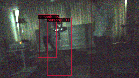
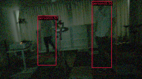
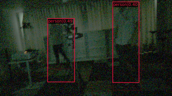
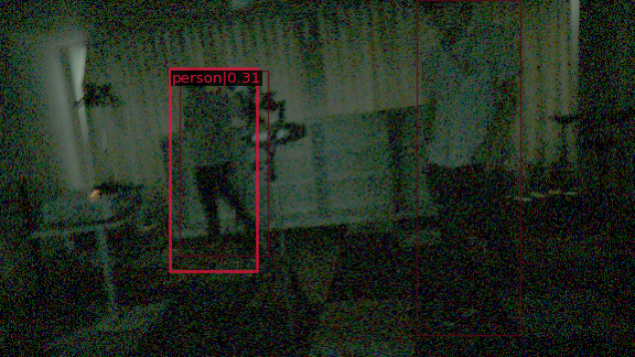
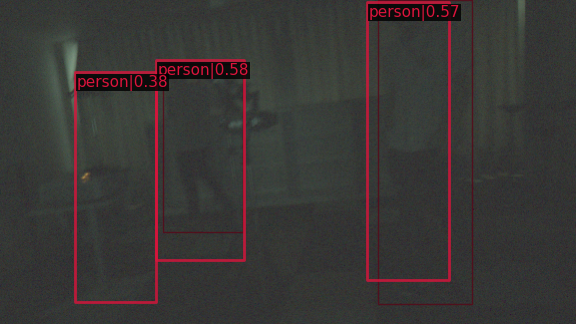
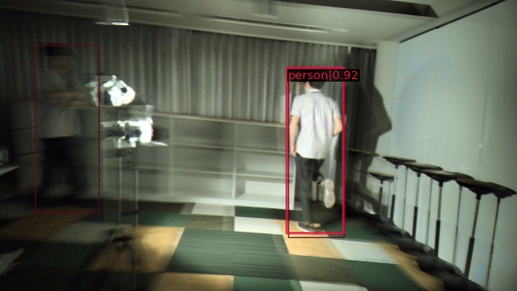
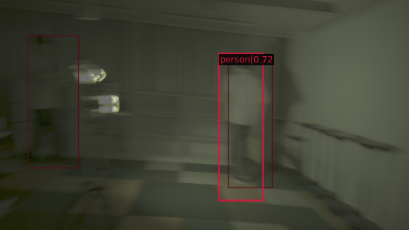
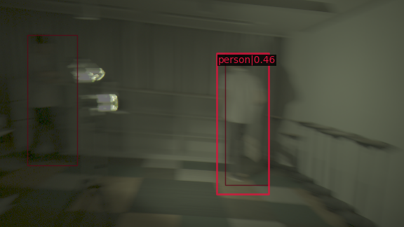
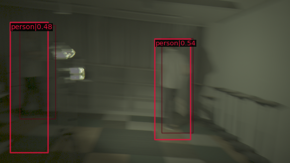
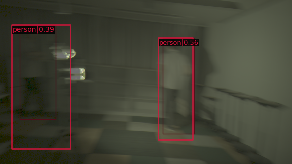
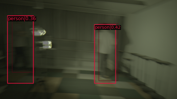
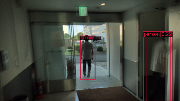
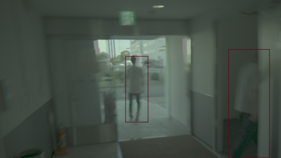
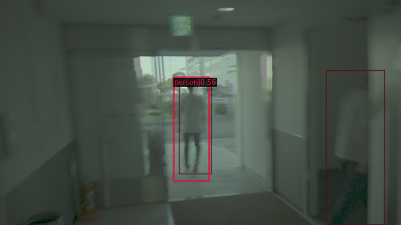
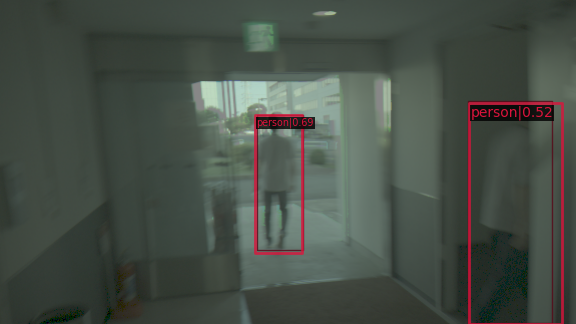
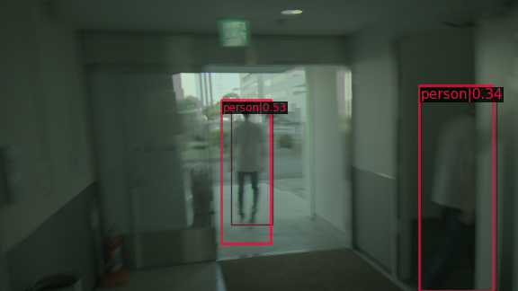
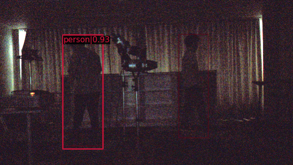
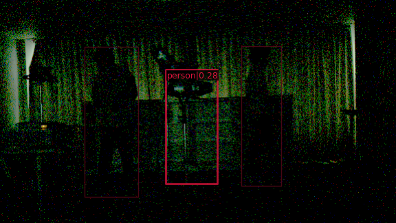
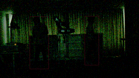
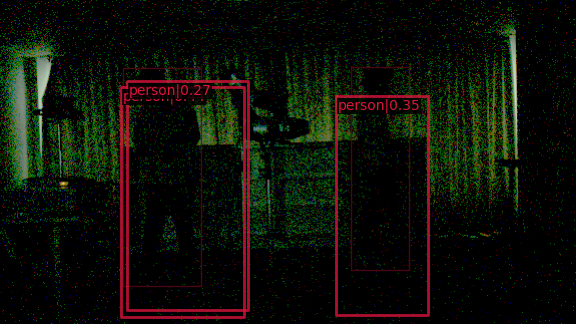
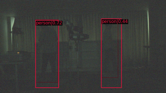
ISP augmentation order noise-accounted	black-box ISP after ISP w/o	simplest gamma after ISP w/o	simplest gamma before ISP (ours) w/o	simplest gamma before ISP (ours) w/o prior	simplest gamma before ISP (ours) w/ (ours)	parameterized gamma before ISP (ours) w/ (ours)

Figure 7: The visualization of the detection results. To make a fair comparison, we set an adequate confidence threshold per model. Specifically, we adjuste the threshold to achieve a precision@0.5 value of 80%. The darker bounding boxes represent the ground truth, while the brighter ones represent the prediction result.

Appendix B Additional Experiments

B.1 Versatility to Different Detectors

TTFNet [28] is used as a detector in the main paper because of the low training cost. In this section, the versatility of the proposed noise-accounted RAW augmentation is checked. As a different type of detector, we choose DeformableDETR [56] as a detector. Also, we change the backbone to ResNet50 [15] to check the proposed method’s effectiveness with a larger model. Furthermore, the backbone is pre-trained with ImageNet [5] to compare with the best accuracy. Other experimental setups are the same as those with TTFNet.

The result is shown in Fig. 4. Because a larger detector with the pre-trained backbone is used, all methods have improved accuracy, but there is still a great improvement from the conventional augmentation after ISP setup to the proposed noise-accounted RAW augmentation when the simplest ISP is used. Moreover, if parameterized gamma tone mapping and the proposed augmentation are used, the accuracy is even improved from the result with the elaborated black-box ISP, which should benefit most from the pre-training with sRGB images.

The future work is to check the effectiveness of the combination of the black-box ISP and the proposed augmentation by implementing the black-box ISP as software that works on a computer.

Table 4: Evaluation with DeformableDETR [56] whose backbone is ResNet50 pre-trained with ImageNet.

			mAP@0.5:0.95 [%]
			black-box	simple ISP
augmentation		noise	ISP	simplest	parameterized
Color + Blur	after	-	51.6	40.2	-
	before (ours)	-	-	46.8	47.5
		ours	-	51.5	52.0

Appendix C Acknowledgements

We would like to thank Aji Widya and Iheb Begalcem for their helpful comments to this manuscript.

References

- [1] Goutam Bhat, Martin Danelljan, Fisher Yu, Luc Van Gool, and Radu Timofte. Deep reparametrization of multi-frame super-resolution and denoising. In Proceedings of the IEEE/CVF International Conference on Computer Vision, pages 2460–2470, 2021.
- [2] Tim Brooks, Ben Mildenhall, Tianfan Xue, Jiawen Chen, Dillon Sharlet, and Jonathan T Barron. Unprocessing images for learned raw denoising. In Proceedings of the IEEE/CVF Conference on Computer Vision and Pattern Recognition, pages 11036–11045, 2019.
- [3] Chen Chen, Qifeng Chen, Jia Xu, and Vladlen Koltun. Learning to see in the dark. In Proceedings of the IEEE conference on computer vision and pattern recognition, pages 3291–3300, 2018.
- [4] Ziteng Cui, Guo-Jun Qi, Lin Gu, Shaodi You, Zenghui Zhang, and Tatsuya Harada. Multitask aet with orthogonal tangent regularity for dark object detection. In Proceedings of the IEEE/CVF International Conference on Computer Vision, pages 2553–2562, 2021.
- [5] Jia Deng, Wei Dong, Richard Socher, Li-Jia Li, Kai Li, and Li Fei-Fei. Imagenet: A large-scale hierarchical image database. In 2009 IEEE conference on computer vision and pattern recognition, pages 248–255. Ieee, 2009.
- [6] Steven Diamond, Vincent Sitzmann, Frank Julca-Aguilar, Stephen Boyd, Gordon Wetzstein, and Felix Heide. Dirty pixels: Towards end-to-end image processing and perception. ACM Transactions on Graphics (TOG), 40(3):1–15, 2021.
- [7] Akshay Dudhane, Syed Waqas Zamir, Salman Khan, Fahad Shahbaz Khan, and Ming-Hsuan Yang. Burst image restoration and enhancement. In Proceedings of the IEEE/CVF Conference on Computer Vision and Pattern Recognition, pages 5759–5768, 2022.
- [8] Abbas El Gamal, Boyd A Fowler, Hao Min, and Xinqiao Liu. Modeling and estimation of fpn components in cmos image sensors. In Solid State Sensor Arrays: Development and Applications II, volume 3301, pages 168–177. SPIE, 1998.
- [9] Martin A Fischler and Robert C Bolles. Random sample consensus: a paradigm for model fitting with applications to image analysis and automated cartography. Communications of the ACM, 24(6):381–395, 1981.
- [10] Alessandro Foi, Mejdi Trimeche, Vladimir Katkovnik, and Karen Egiazarian. Practical poissonian-gaussian noise modeling and fitting for single-image raw-data. IEEE Transactions on Image Processing, 17(10):1737–1754, 2008.
- [11] Ian Goodfellow, Jean Pouget-Abadie, Mehdi Mirza, Bing Xu, David Warde-Farley, Sherjil Ozair, Aaron Courville, and Yoshua Bengio. Generative adversarial nets. Advances in neural information processing systems, 27, 2014.
- [12] Ryan D Gow, David Renshaw, Keith Findlater, Lindsay Grant, Stuart J McLeod, John Hart, and Robert L Nicol. A comprehensive tool for modeling cmos image-sensor-noise performance. IEEE Transactions on Electron Devices, 54(6):1321–1329, 2007.
- [13] Chunle Guo, Chongyi Li, Jichang Guo, Chen Change Loy, Junhui Hou, Sam Kwong, and Runmin Cong. Zero-reference deep curve estimation for low-light image enhancement. In Proceedings of the IEEE/CVF Conference on Computer Vision and Pattern Recognition, pages 1780–1789, 2020.
- [14] Patrick Hansen, Alexey Vilkin, Yury Krustalev, James Imber, Dumidu Talagala, David Hanwell, Matthew Mattina, and Paul N Whatmough. Isp4ml: The role of image signal processing in efficient deep learning vision systems. In 2020 25th International Conference on Pattern Recognition (ICPR), pages 2438–2445. IEEE, 2021.
- [15] Kaiming He, Xiangyu Zhang, Shaoqing Ren, and Jian Sun. Deep residual learning for image recognition. In Proceedings of the IEEE conference on computer vision and pattern recognition, pages 770–778, 2016.
- [16] Yang Hong, Kaixuan Wei, Linwei Chen, and Ying Fu. Crafting object detection in very low light. In Proceedings of the British Machine Vision Virtual Conference, 2021.
- [17] Andrey Ignatov, Nikolay Kobyshev, Radu Timofte, Kenneth Vanhoey, and Luc Van Gool. Dslr-quality photos on mobile devices with deep convolutional networks. In Proceedings of the IEEE International Conference on Computer Vision, pages 3277–3285, 2017.
- [18] Andrey Ignatov, Luc Van Gool, and Radu Timofte. Replacing mobile camera isp with a single deep learning model. In Proceedings of the IEEE/CVF Conference on Computer Vision and Pattern Recognition Workshops, pages 536–537, 2020.
- [19] Tomas Jenicek and Ondrej Chum. No fear of the dark: Image retrieval under varying illumination conditions. In Proceedings of the IEEE/CVF International Conference on Computer Vision, pages 9696–9704, 2019.
- [20] Haiyang Jiang and Yinqiang Zheng. Learning to see moving objects in the dark. In Proceedings of the IEEE/CVF International Conference on Computer Vision, pages 7324–7333, 2019.
- [21] Yifan Jiang, Xinyu Gong, Ding Liu, Yu Cheng, Chen Fang, Xiaohui Shen, Jianchao Yang, Pan Zhou, and Zhangyang Wang. Enlightengan: Deep light enhancement without paired supervision. IEEE Transactions on Image Processing, 30:2340–2349, 2021.
- [22] Brian L Joiner and Joan R Rosenblatt. Some properties of the range in samples from tukey’s symmetric lambda distributions. Journal of the American Statistical Association, 66(334):394–399, 1971.
- [23] Diederik P Kingma and Jimmy Ba. Adam: A method for stochastic optimization. arXiv preprint arXiv:1412.6980, 2014.
- [24] Mikhail Konnik and James Welsh. High-level numerical simulations of noise in ccd and cmos photosensors: review and tutorial. arXiv preprint arXiv:1412.4031, 2014.
- [25] Tsung-Yi Lin, Michael Maire, Serge Belongie, James Hays, Pietro Perona, Deva Ramanan, Piotr Dollár, and C Lawrence Zitnick. Microsoft coco: Common objects in context. In European conference on computer vision, pages 740–755. Springer, 2014.
- [26] Shuai Liu, Chaoyu Feng, Xiaotao Wang, Hao Wang, Ran Zhu, Yongqiang Li, and Lei Lei. Deep-flexisp: A three-stage framework for night photography rendering. In Proceedings of the IEEE/CVF Conference on Computer Vision and Pattern Recognition, pages 1211–1220, 2022.
- [27] Xinhao Liu, Masayuki Tanaka, and Masatoshi Okutomi. Practical signal-dependent noise parameter estimation from a single noisy image. IEEE Transactions on Image Processing, 23(10):4361–4371, 2014.
- [28] Zili Liu, Tu Zheng, Guodong Xu, Zheng Yang, Haifeng Liu, and Deng Cai. Training-time-friendly network for real-time object detection. In proceedings of the AAAI conference on artificial intelligence, volume 34, pages 11685–11692, 2020.
- [29] Ilya Loshchilov and Frank Hutter. Sgdr: Stochastic gradient descent with warm restarts. arXiv preprint arXiv:1608.03983, 2016.
- [30] Feifan Lv, Feng Lu, Jianhua Wu, and Chongsoon Lim. Mbllen: Low-light image/video enhancement using cnns. In BMVC, volume 220, page 4, 2018.
- [31] Long Ma, Tengyu Ma, Risheng Liu, Xin Fan, and Zhongxuan Luo. Toward fast, flexible, and robust low-light image enhancement. In Proceedings of the IEEE/CVF Conference on Computer Vision and Pattern Recognition, pages 5637–5646, 2022.
- [32] Markku Makitalo and Alessandro Foi. Optimal inversion of the generalized anscombe transformation for poisson-gaussian noise. IEEE transactions on image processing, 22(1):91–103, 2012.
- [33] Kristina Monakhova, Stephan R Richter, Laura Waller, and Vladlen Koltun. Dancing under the stars: video denoising in starlight. In Proceedings of the IEEE/CVF Conference on Computer Vision and Pattern Recognition, pages 16241–16251, 2022.
- [34] Igor Morawski, Yu-An Chen, Yu-Sheng Lin, Shusil Dangi, Kai He, and Winston H Hsu. Genisp: Neural isp for low-light machine cognition. In Proceedings of the IEEE/CVF Conference on Computer Vision and Pattern Recognition, pages 630–639, 2022.
- [35] Ali Mosleh, Avinash Sharma, Emmanuel Onzon, Fahim Mannan, Nicolas Robidoux, and Felix Heide. Hardware-in-the-loop end-to-end optimization of camera image processing pipelines. In Proceedings of the IEEE/CVF Conference on Computer Vision and Pattern Recognition, pages 7529–7538, 2020.
- [36] Emmanuel Onzon, Fahim Mannan, and Felix Heide. Neural auto-exposure for high-dynamic range object detection. In Proceedings of the IEEE/CVF Conference on Computer Vision and Pattern Recognition, pages 7710–7720, 2021.
- [37] Abhijith Punnappurath, Abdullah Abuolaim, Abdelrahman Abdelhamed, Alex Levinshtein, and Michael S Brown. Day-to-night image synthesis for training nighttime neural isps. In Proceedings of the IEEE/CVF Conference on Computer Vision and Pattern Recognition, pages 10769–10778, 2022.
- [38] Erik Reinhard, Wolfgang Heidrich, Paul Debevec, Sumanta Pattanaik, Greg Ward, and Karol Myszkowski. High dynamic range imaging: acquisition, display, and image-based lighting. Morgan Kaufmann, 2010.
- [39] Yukihiro Sasagawa and Hajime Nagahara. Yolo in the dark-domain adaptation method for merging multiple models. In European Conference on Computer Vision, pages 345–359. Springer, 2020.
- [40] Eli Schwartz, Alex Bronstein, and Raja Giryes. Isp distillation. arXiv preprint arXiv:2101.10203, 2021.
- [41] Samuel S Shapiro and RS Francia. An approximate analysis of variance test for normality. Journal of the American statistical Association, 67(337):215–216, 1972.
- [42] Sungho Suh, Shinya Itoh, Satoshi Aoyama, and Shoji Kawahito. Column-parallel correlated multiple sampling circuits for cmos image sensors and their noise reduction effects. Sensors, 10(10):9139–9154, 2010.
- [43] Justin Tomasi, Brandon Wagstaff, Steven L Waslander, and Jonathan Kelly. Learned camera gain and exposure control for improved visual feature detection and matching. IEEE Robotics and Automation Letters, 6(2):2028–2035, 2021.
- [44] Zhengzhong Tu, Hossein Talebi, Han Zhang, Feng Yang, Peyman Milanfar, Alan Bovik, and Yinxiao Li. Maxim: Multi-axis mlp for image processing. In Proceedings of the IEEE/CVF Conference on Computer Vision and Pattern Recognition, pages 5769–5780, 2022.
- [45] Yuzhi Wang, Haibin Huang, Qin Xu, Jiaming Liu, Yiqun Liu, and Jue Wang. Practical deep raw image denoising on mobile devices. In European Conference on Computer Vision, pages 1–16. Springer, 2020.
- [46] Zhixiang Wang, Xiang Ji, Jia-Bin Huang, Shin’ichi Satoh, Xiao Zhou, and Yinqiang Zheng. Neural global shutter: Learn to restore video from a rolling shutter camera with global reset feature. In Proceedings of the IEEE/CVF Conference on Computer Vision and Pattern Recognition, pages 17794–17803, 2022.
- [47] Chen Wei, Wenjing Wang, Wenhan Yang, and Jiaying Liu. Deep retinex decomposition for low-light enhancement. arXiv preprint arXiv:1808.04560, 2018.
- [48] Kaixuan Wei, Ying Fu, Jiaolong Yang, and Hua Huang. A physics-based noise formation model for extreme low-light raw denoising. In Proceedings of the IEEE/CVF Conference on Computer Vision and Pattern Recognition, pages 2758–2767, 2020.
- [49] Jay Whang, Mauricio Delbracio, Hossein Talebi, Chitwan Saharia, Alexandros G Dimakis, and Peyman Milanfar. Deblurring via stochastic refinement. In Proceedings of the IEEE/CVF Conference on Computer Vision and Pattern Recognition, pages 16293–16303, 2022.
- [50] Chyuan-Tyng Wu, Leo F Isikdogan, Sushma Rao, Bhavin Nayak, Timo Gerasimow, Aleksandar Sutic, Liron Ain-kedem, and Gilad Michael. Visionisp: Repurposing the image signal processor for computer vision applications. In 2019 IEEE International Conference on Image Processing (ICIP), pages 4624–4628. IEEE, 2019.
- [51] Syed Waqas Zamir, Aditya Arora, Salman Khan, Munawar Hayat, Fahad Shahbaz Khan, Ming-Hsuan Yang, and Ling Shao. Cycleisp: Real image restoration via improved data synthesis. In Proceedings of the IEEE/CVF Conference on Computer Vision and Pattern Recognition, pages 2696–2705, 2020.
- [52] Hongguang Zhang, Yuchao Dai, Hongdong Li, and Piotr Koniusz. Deep stacked hierarchical multi-patch network for image deblurring. In Proceedings of the IEEE/CVF Conference on Computer Vision and Pattern Recognition, pages 5978–5986, 2019.
- [53] Meina Zhang, Yingying Fang, Guoxi Ni, and Tieyong Zeng. Pixel screening based intermediate correction for blind deblurring. In Proceedings of the IEEE/CVF Conference on Computer Vision and Pattern Recognition, pages 5892–5900, 2022.
- [54] Yi Zhang, Dasong Li, Ka Lung Law, Xiaogang Wang, Hongwei Qin, and Hongsheng Li. Idr: Self-supervised image denoising via iterative data refinement. In Proceedings of the IEEE/CVF Conference on Computer Vision and Pattern Recognition, pages 2098–2107, 2022.
- [55] Yonghua Zhang, Jiawan Zhang, and Xiaojie Guo. Kindling the darkness: A practical low-light image enhancer. In Proceedings of the 27th ACM international conference on multimedia, pages 1632–1640, 2019.
- [56] Xizhou Zhu, Weijie Su, Lewei Lu, Bin Li, Xiaogang Wang, and Jifeng Dai. Deformable detr: Deformable transformers for end-to-end object detection. arXiv preprint arXiv:2010.04159, 2020.