An Online Learning Approach for Vehicle Usage Prediction During COVID-19

Abstract

Today, there is an ongoing transition to more sustainable transportation, and an essential part of this transition is the switch from combustion engine vehicles to battery electric vehicles (BEVs). BEVs have many advantages from a sustainability perspective, but issues such as limited driving range and long recharge times slow down the transition from combustion engines. One way to mitigate these issues is by performing battery thermal preconditioning, which increases the energy efficiency of the battery. However, to optimally perform battery thermal preconditioning, the vehicle usage pattern needs to be known, i.e., how and when the vehicle will be used. This study attempts to predict the departure time and distance of the first drive each day using different online machine learning models. The online machine learning models are trained and evaluated on historical driving data collected from a fleet of BEVs during the COVID-19 pandemic. Additionally, the prediction models are extended to quantify the uncertainty of their predictions, which can be used as guidance to whether the prediction should be used or dismissed. We show that the best-performing prediction models yield an aggregated mean absolute error of 2.75 hours when predicting departure time and 13.37 km when predicting trip distance.

I Introduction

There is currently an ongoing transition to more sustainable transportation. Recently, there have been several initiatives that aim to reduce greenhouse gas emissions from vehicles and further accelerate the transition to zero-emission vehicles. The European Commission has, for example, proposed a 55 % reduction of emissions from cars by 2030 and zero emissions from new cars by 2035 [1]. Furthermore, several governments, cities, and automotive manufacturers have recently committed to work towards only allowing zero emission vehicles to be sold in the leading markets by 2035 and globally by 2040 [2]. In California, an executive order has been issued requiring every new sale of passenger vehicles to be emission free by 2035 [3].

An essential step in the switch to a more sustainable transportation system is battery electric vehicles (BEV s). BEV s are pure electric vehicles and make up two-thirds of the rapidly growing global electric car stock [4]. While production of electric vehicles may produce emissions, usage is emission free as long as the energy sources used for charging do not emit greenhouse gases.

However, even though BEV s have many advantages from a sustainability perspective, they face other challenges. Compared to vehicles with a combustion engine, BEV s have a more limited driving range and longer recharge times. These disadvantages are exacerbated in cold and hot climates due to harsher driving conditions, making propulsive consumption increase. Additionally, in these conditions, auxiliary consumption generally increase to keep satisfactory comfort when driving, especially in colder temperatures [5, 6]. There are several strategies to mitigate the effects caused by the climate conditions, e.g., cabin preconditioning before departure, battery thermal preconditioning before fast charging, or battery thermal preconditioning before departure. Furthermore, the charging scheduling could be optimized, as the time of day affects the cost and carbon dioxide footprint of the electricity production.

To perform all these different kinds of strategies, it is, however, needed to first learn about the vehicle usage pattern, i.e., how and when the vehicle will be used the next time. Some of this information, such as departure time and driving distance, can be given by the driver. However, it might not be convenient for the driver to fill in information about the next drive, and even if they do, it might not be accurate. Therefore, a better way to acquire the needed information may be to use historical data and machine learning to predict when and how the vehicle will be used in the near future. Consequently, this study explores how accurately different machine learning models can predict vehicle usage patterns. More specifically, we attempt to predict departure times and driving distances in this study.

The data used in this study arrive over time, and as argued in [7], a specific type of machine learning, called online learning, fits well with this setting. Online learning is a machine learning paradigm that continuously updates the models as new data arrive over time, and subsequently discards the data after the model has been updated. This way, the machine learning models may function in environments with limited data storage and computational power. These characteristics could allow us to implement the prediction models on the BEV s directly, avoiding the need to transfer sensitive user data over the network.

In the literature, there seems to be a lack of consensus on the precise definition of online learning, and it is often intertwined with a similar paradigm called incremental learning [8, 9, 10, 7]. To make these concepts clear, in this paper we refer to online learning as the concept of training sequentially on a single observation or a limited sequence of past observations.

The main contributions of this paper are summarized as follows:

• To the best of our knowledge, no research has been made on predicting vehicle usage using online learning models. Thus, this paper introduces a new perspective by considering the utilization of novel and efficient prediction methods in computationally constrained environments, such as in the internal electronic control units (ECU s) of a vehicle.

• This work utilizes novel approaches to estimate the quality of the predictions, which could enable the vehicle to invalidate uncertain predictions without any human intervention.

• We introduce a new approach of estimating whether the vehicle has recurrent behavior by using the clustering tendency of the departure times and driving distances.

• This work also considers prediction of driving behavior during the COVID-19 pandemic, where the studied non-public real-world data set covers more than 300 BEV s driven by employees of Volvo Car Corporation over the course of an entire year. To our knowledge, no work has performed such a comprehensive analysis of predicting vehicle usage during COVID-19, where commutes are increasingly irregular.

The rest of this paper is organized as follows; Section II covers related work studying similar prediction problems, however, in possibly different contexts. Section III concretizes the aim of the paper. Section IV describes the origin of the data and the preprocessing steps. In Section VI, the prediction models are described together with the validation procedure. Section VII covers the results from predicting driving distance and departure time, together with a discussion, and Section VIII concludes the paper and suggests some future directions.

II Related Work

As mentioned in the introduction, this study investigates how well a vehicle’s departure times and driving distances can be predicted. This subsection introduces related articles and papers where departure time and trip distance forecasts have been performed using various machine learning models. However, none of the presented papers considers using online learning models, and to the best of our knowledge, no research has been performed regarding prediction of vehicle usage using online models.

II-A Departure Time Prediction

Intuitively, the forecast for individual BEV s should depend highly on the driver, compared to e.g., busses which follow a fixed schedule. Considering an office commute, where flexible working hours are often applied, the arrival time to the office could vary significantly, which implicitly should affect the departure time from the office as well. This type of correlation is shown in [11], where the authors predict the departure times from workplaces, to optimize smart charging. The authors point out that the average departure time of a BEV has a standard deviation of 141 minutes, showcasing the difficulty of this task. They investigate several different regression models on historical charging data and observe that sophisticated algorithms like XGBoost and artificial neural networks perform better than linear models, receiving a mean absolute error of 82 minutes. In [12] The authors predict the starting time and end time of an upcoming trip based on the start time, end time, and distance of the most recent previous trip. They receive a root mean square error (RMSE) of around 2 hours for both the start and end time. The authors also argue that simpler models such as KNN and decision trees outperform more complex neural-network-based models, even though the more complex models are better at extracting the travel behavior. Other approaches to departure forecasting predict time intervals instead of a specific time. For example, [13] forecasts a time interval of 15 minutes, resulting in an RMSE of roughly 3 hours.

The authors of [14] investigate the variation of departure times and attempt to model the first daily departure time as a probability distribution. They state that this is impossible after applying statistical tests measuring the similarity of well-known probability distributions.

II-B Trip Distance Prediction

Trip distance is an important factor to know certain characteristics of the trip, and can be useful when, e.g., deciding whether battery thermal preconditioning is beneficial or not. Panahi et al. [15] predict the driving distance using artificial neural networks, resulting in a mean absolute deviation (MAD) of around 9%. Baghali et al. [12] implement a range of machine learning models, such as K-Nearest Neighbours (KNN), decision trees, random forest, and a range of neural networks, for predicting the daily travel and charging demand of electric vehicles. The novelty in their work is that they considered charging at more places than at home. They show that even the less complex models generate reasonable results, with an RMSE of around 19-23 km. However, they point out that to find daily temporal patterns, more complex models are needed.

As the authors of [14] state, different individuals may have different driving patterns. The authors of [16] cluster plug-in electric vehicle owners according to patterns in their driving behaviors. They train two Long Short-Term Memory (LSTM)recurrent neural networks on each cluster to forecast arrival time and travel distance, and subsequently investigate the financial impacts of charging demand using these predictions. The authors show a significant improvement in forecasting the travel distance when the driving behavior is tied to a specific travel behavior pattern.

II-C Driving Patterns During COVID-19

The COVID-19 pandemic has had major impacts on people’s everyday lives and how they travel. Not only due to the severity of the disease, but also how authorities enforced restrictions to counter the spread of the pandemic. Interestingly, [17] and [18] found that the vehicle charging behavior was affected by the level of restrictions enforced, where the charging activity increased as restrictions were lifted.

To deal with the restrictions, various workplaces started to opt for teleworking [19, 20, 21, 22, 23]. In fact, a survey in Canada shows that the amount of people working remotely increased five-fold [19, 20], while the number of people who commuted decreased slightly compared to the pre-pandemic period. A survey of public agencies in Sweden found that people who commuted 4-5 times a week pre-pandemic barely commuted once a week during the pandemic, due to teleworking [21]. Further, it was reported the 86% of the people changed commuting behavior during the pandemic, despite the relatively liberal restrictions in Sweden. In a large study of travel behavior, [23] included a survey of how people expected to commute in the future. It was reported that 48% anticipate having the option to work from home, and that it is expected that people will commute 3.42 times per week, which is a 17% decline from the pre-pandemic period.

The decrease in commuting trips has paved the path for new behaviors. [19, 20] found that despite the decrease in commuting, the total number of trips increased. One reason for this might be that the time employees save by not commuting is used to perform other kinds of trips [24], [21].

III Problem Statement

To concretize what this study aims to address, we define the following research question:

How accurately can online learning models predict the departure time and distance of an upcoming drive?

We address this question by comparing several online machine learning models in terms of error rate, as well as how uncertain the models are in their predictions. The uncertainty is an important aspect since it can be essential to know how confident the model is when a prediction is used to make a critical decision.

The online learning problem is defined as follows: For each time step $t$, where $t$ corresponds to a day, a feature vector $\textbf{x}_{t}$ is received by a prediction model $M_{t}$ at midnight. The model $M_{t}$ is expected to predict the target $y_{t}$, which can be either the time from midnight to the first departure time, or the driving distance of the first drive. When the true value of the target $y_{t}$ becomes available, the task is to infer a model $M_{t+1}$ only based on $(\textbf{x}_{t},y_{t})$ and $M_{t}$. The model $M_{t+1}$ is then used in the next time step.

To limit the scope of the study, focus is put on commuting drives. For this reason, we only consider the first drive of each day for predictions. It is assumed that each prediction is performed at midnight and that it is known whether there will be a drive or not on that specific day. Further, the predictions are performed individually for each vehicle, i.e., each vehicle has its own prediction model. Online learning has, as mentioned earlier, the benefit of potentially being implemented in the ECU s of the vehicles, as it is able to operate in a system with limited computational resources. Actual implementation in vehicles is however not considered in this work, as the aim is only to investigate whether it is plausible to predict vehicle usage using online learning.

IV Data

The data used to train and evaluate the prediction models are collected from a fleet of BEV s driven by Volvo Car Corporation employees in their everyday life, where each employee has signed an agreement allowing use of the data for research purposes. No personal or sensitive data have been accessed or used for this study. The data consist of pseudonymised measurements of different attributes such as velocity, acceleration, the state of charge (SoC), and energy consumption. These attributes are measured at a constant rate with high frequency during measurement sessions and give a granular view of the car’s properties. From these measurements, we extract summaries of the driving and charging sessions, and use them as input to the prediction models. These summaries consist of aggregations of the attributes, such as mean, standard deviation, maximum and minimum value. To shortly describe the trends of the variables we intend to predict, it can be seen that most of the trips in the dataset are short, with a mean distance of 23.1 km and a median distance of 13.3 km. The departure time varies a bit more, with a peak at roughly 7.5 a.m., but a mean departure time at 10.42 p.m.

IV-A Preprocessing

To increase the data quality, we apply several filters to the summarizations of driving and charging sessions. These filters are described in the list below and handle inconsistencies such as missing data and abnormally short or long sessions.

• All driving and charging sessions shorter than 50 seconds are removed. The selection of 50 seconds is arbitrary, though it removes most of the anomalous short trips and charging sessions.

• Two subsequent drive or charging sessions are merged if there are less than 15 minutes between them. This mainly affects the driving sessions, and we argue that this provides a better overview of the vehicle usage and that a 15-minute break should not break one drive into two.

• Vehicles with less than 50 drives are removed from the data to ensure that there exists a minimum of drives for each vehicle from which the prediction models can attempt to learn.

IV-B Features considered

As mentioned previously, the predictions of departure time and trip distance are based on aggregations of different signals. Below, the signals considered for the prediction of the target variables are presented, with a short argument of why we consider them useful.

• Date of when prediction is performed. It is reasonable to assume that the date of the prediction will affect when the first trip of the day. For example, it is reasonable that the first drive occurs earlier on a Monday than on a Saturday.

• Start time, end time, and distance of the previous trip. These metrics should help to understand the recent vehicle usage and might indicate what the next trip will be. E.g., for some drivers, short shopping trips might be likely to follow directly after longer commutes in the afternoon.

• Start time of most recent charging session. The start time of the most recent charging session may provide useful information about driver patterns, since charging sessions at different parts of the day can give indications about the intent of the driver.

• State of charge at the beginning of most recent charging session. The state of charge at the beginning of the most recent charging session may enhance any insights about the driver pattern gained from knowing the start time of the most recent charge.

• Ambient temperature and sun load during the previous trip. The current weather could affect vehicle usage. A trip during the weekend may be more likely if it seems to be warm and sunny outside. However, while this data could be provided by a third party, in this study we attempt to only use information from the vehicle.

• Speed and acceleration during the previous trip. The average, standard deviation, min and max of the speed and acceleration of the previous trip may indicate if the trip was a city or a highway drive, or something else. The acceleration might further indicate the driving behavior and possibly, if several people are sharing the car, who was driving.

• State of charge during the previous trip. Along with the previously mentioned features, such as trip distance, the change of state of charge during the last trip may provide some information about e.g., road type, which might help in predicting the next trip.

Beyond the presented features, we perform feature engineering to extract further information from the temporal features and the previous target variables. Starting with the temporal features, we extract the minute of the hour, the hour of the day, the part of the day (morning, noon, afternoon, etc.), the day of the month, the day of the week, whether it is a workday or not, similar to [11]. The features that are categorical by nature, e.g., part of day, are considered as one-hot encodings. Further, cyclic representations are extracted from some of the continuous temporal variables. This is done by performing the trigonometric transformations

$$f_{x}=\sin(2\pi f/\max(f)),$$ (1)

$$f_{y}=\cos(2\pi f/\max(f)),$$ (2)

where $f$ is the feature to be transformed and $f_{x}$ and $f_{y}$ are the two components of the cyclic feature [25]. Lastly, inspired by [25, 11], historical averages and running averages of the past target variables are introduced.

V Prediction Models

In this section, we introduce several online machine learning models we adapt to predict the departure time and distance of an upcoming drive. Furthermore, as an additional step to see the effects on changing user behavior, the uncertainty of the predictions is investigated as well.

To quantify the uncertainty of a prediction, one may use prediction intervals. A prediction interval quantifies a potential range where a future observation will occur with a certain probability. For instance, when using a 95% prediction interval, we expect that the next observation will fall within the prediction interval with a 95% certainty.

A prediction interval may be defined as

$$[\hat{y}-z_{\frac{\tau}{2}}\sigma,\hat{y}+z_{\frac{\tau}{2}}\sigma],$$ (3)

where $\hat{y}$ is the model prediction, $z_{\frac{\tau}{2}}$ is the upper $\frac{\tau}{2}$ quantile of a standard normal distribution and $\sigma$ is the prediction standard error [26].

V-A Historical Average

As a baseline, we use the historical average to predict the departure time and trip distance. This method is incremental by nature, as it keeps track of the average departure time and trip distance over time.

V-B Quantile Regression

The first machine learning model we study is an online version of the quantile linear regression model. Ordinary linear regression defined as

$$\hat{y}=\theta^{T}\textbf{x},$$ (4)

where $\hat{y}$ is the predicted target, x is the observed feature vector and $\theta$ is the weight vector. The weight vector may be updated incrementally using stochastic gradient descent (SGD) in the following way:

$$\theta^{(i+1)}=\theta^{(i)}-\eta\nabla(\mathcal{L}(y,\textbf{x},\theta^{(i)})+(\theta^{(i)})^{T}(\theta^{(i)})\lambda),$$ (5)

where $\lambda$ is a regularization parameter, and $\mathcal{L}(y,\textbf{x},\theta^{(i)})$ is the loss function with the true target $y$, the observed feature vector x and the current weight vector $\theta^{(i)}$. Using the squared loss, the predicted target will be the conditional mean. However, by changing the loss to the tilted absolute value function, we may predict a specified quantile instead. The tilted absolute value function is defined as

$$L_{\tau}(y,\textbf{x},\theta)=\begin{cases}(\tau-1)(y-\theta^{T}\textbf{x})&\textrm{ if }y<\theta^{T}\textbf{x},\\ \tau(y-\theta^{T}\textbf{x})&\textrm{ if }y\geq\theta^{T}\textbf{x},\end{cases}$$ (6)

where $\tau$ is the chosen quantile [27, 28]. Using this function, the inference is divided into two parts. The inferred prediction by the model is the median, i.e., the $50^{\textrm{th}}$ quantile, while the uncertainty is defined by predicting the $5^{\textrm{th}}$ and the $95^{\textrm{th}}$ quantiles using the tilted absolute value function, resulting in $\hat{y}-z_{\frac{\tau}{2}}\sigma$ and $\hat{y}+z_{\frac{\tau}{2}}\sigma$ respectively in Equation 3.

V-C Quantile K-Nearest Neighbours

The second machine learning model is an adjusted version of the K-Nearest Neighbours (KNN) method. A prediction $\hat{y}$ is calculated by taking the mean of the closest $K$ neighbors:

$$\hat{y}=\frac{1}{K}\sum_{\textbf{x}_{i}\in N_{k}(\textbf{x})}y_{i},$$ (7)

where $N_{k}(\textbf{x})$ is the set of seen observations closest to the new observation, and $y_{i}$ is the target value corresponding to observation $\textbf{x}_{i}$ in the set $N_{k}(\textbf{x})$. A typical way of measuring the distance between observations is to use the Euclidean distance in the feature space [29, pp. 14–16]. The KNN model is made online by only using the $N$ latest observations, where $N$ is a tunable hyperparameter.

The quantiles in Equation 3 are estimated by fitting a Gaussian distribution on the $K$ nearest neighbours and using the standard deviation of that distribution in Equation 3 [30].

V-D Quantile Adaptive Random Forest

The third machine learning model is a modified version of Random Forest [29, pp. 305–307]. To make it online, we use incremental Hoeffding trees as base-learners [31, 32]. Hoeffding trees are described in [33], and can determine, with a certain confidence, the number of observations needed to select the optimal splitting feature. In our setting, the feature to split at a specific node is the one reducing the variance in the target space the most [34, 35]. Furthermore, to make the online Random Forest more responsive to changes in the data, we use an algorithm called the Adaptive Windowing to retrain a new version of the model in the background if a potential shift in data distribution is detected.

The online Random Forest is then modified further for uncertainty estimation, using the method of Vasiloudis et al. [36]. Their approach is to keep an approximated representation of the observed target values, from which it is possible to extract percentiles at desired significance levels. To bound the memory required for storage of the approximation, the authors use an incremental and mergeable data structure called a KLL sketch. They let each leaf in the forest store a sketch, which keeps an approximation of the target values with a small memory footprint. When the forest receives a new training instance, each tree sorts the instance to a leaf, and updates the leaf’s sketch with the target of the training instance. The prediction process makes use of the approximated target values to create a prediction interval. Each tree sorts the input to a leaf, and all the sketches of the reached leafs are merged. From the merged sketch we fit a Gaussian distribution, and use the standard deviation of this distribution in Equation 3.

V-E Feed-Forward Neural Network with Uncertainty Quantification

The last machine learning model we study is a Feed Forward Neural Network, where each hidden layer $h$ is defined by

$$h_{i+1}=g(W^{T}h_{i}+b)$$ (8)

where $W$ and $b$ are learnable parameters and $g(\cdot)$ is a non-linear activation function. This is made online by only using a single observation at a time when performing back propagation to train the network, hence, training it sequentially as new observations are observed.

When quantifying uncertainty, it is common to differentiate between two different kinds of uncertainty: aleatoric and epistemic [37, pp. 7–9], [38, 26, 39, 40, 41]. Aleatoric uncertainty corresponds to the uncertainty present in the data, such as noise. However, it could also be due to hidden variables that affect the prediction outcome (in the context of our work, a hidden variable could, for example, be information about upcoming meetings at work). On the other hand, epistemic uncertainty corresponds to the uncertainty due to the prediction model being inexperienced in certain regions of the data distribution.

To quantify the uncertainty in each prediction, we take inspiration of [26], who aggregate the epistemic and aleatoric uncertainties to estimate the standard error used in Equation 3. The epistemic uncertainty is estimated using a technique called Monte Carlo Dropout, introduced in [42]. In short, multiple predictions are performed using the same observation, where each prediction is individually affected by dropout. This means that some of the neurons in each layer are disregarded for each prediction, resulting in varying outputs. From a Bayesian perspective, the outputs can be seen as samples from the posterior predictive distribution. The authors prove that this posterior estimation approximates a Gaussian process, where the variance of the process corresponds to the uncertainty, approximated as

$$\hat{\sigma}^{2}_{e}=\frac{1}{B}\sum_{b=1}^{B}(\hat{y}_{b}-\bar{\hat{y}})^{2},$$ (9)

where $B$ is the number of predictions, and $\bar{\hat{y}}$ is the average of the predictions $\hat{y}_{b}$, where $b\in[B]$. The aleatoric uncertainty is estimated from the residual sum of squares of the 10 latest predictions, given by

$$\hat{\sigma}^{2}_{a}=\frac{1}{10}\sum_{i=1}^{10}(y_{i}-\hat{y}_{i})^{2}.$$ (10)

Finally, the total uncertainty is calculated by

$$\hat{\sigma}^{2}=\sqrt{\hat{\sigma}^{2}_{e}+\hat{\sigma}^{2}_{a}},$$ (11)

which effectively represents the standard error in Equation 3.

VI Prediction Process

As mentioned in Section I, we use an online learning approach in this study, as it fits well with the sequential nature of the data, where new observations become available over time. The online learning approach enables continuous learning over time and avoids the need to retrain the model when new samples become available. However, a negative aspect of this approach is the lack of a standardized way of performing feature selection and hyperparameter optimization [43]. The authors of [7] present two approaches for hyperparameter optimization. The first approach is called the offline setting, where a complete training set is used to find the hyperparameters, much like in the traditional machine learning paradigm. The optimal hyperparameters are subsequently used to validate the models on a test set. The second approach, called the online setting, saves the first 20% (or the first 1000) observations in a buffer to perform hyperparameter tuning on. The second approach does, however, make the assumptions that the selection of these hyperparameters is optimal throughout the rest of the stream and that concept drifts do not occur [43].

In addition to online learning, this study also uses personalized models, i.e., there is one model instance per vehicle. This setup makes feature and hyperparameter selection more challenging, as the features and parameters yielding the best results might differ among vehicles. We simplify the selection of hyperparameters and features for each machine learning model by selecting the ones yielding the lowest average MAE for all cars. The selection method is similar to the first approach described in [7]. That is, feature selection and hyperparameter tuning for a model are performed on a subset of the vehicles. The selected features and hyperparameters are then used on the remaining vehicles to evaluate the models.

VI-A Selecting Well-behaving Vehicles

The vehicles used in the feature and hyperparameter selection, and the vehicles used in the evaluation of the prediction models, are not selected completely at random. Analysis of the target variables indicates that the occurrence of recurrent vehicle usage varies greatly between different vehicles, potentially making the usage patterns of some cars more difficult to predict than that of others. Inspired by Goebel and Voß [14], we want to focus on the vehicles that, despite the COVID-19 pandemic, have some regularity in the usage pattern. In their work, they predict the first daily departure time of commuter vehicles, and develop a selection method for finding “well-behaving” vehicles. The goal of this selection method is to find vehicles that regularly travel to work and have similar departure times each day. They do this by selecting vehicles with a low variance in the departure time and the number of weekdays where drives occur.

One problem with utilizing the same approach in this study is that it might favor cars with a similar departure time every day, and disregard cars whose departure times vary per day but are the same across weeks. To also capture the weekly patterns, we want to find cars where similar observations of departure times and trip distances are frequently observed. Therefore, we propose a different selection method, where the clustering tendency is measured, i.e., how well the data can be clustered. A strong clustering tendency indicates that similar observations are frequently observed and that a recurrent vehicle usage pattern exists.

The clustering tendency is measured by a statistical test called the Hopkins test [44]. The test compares the joint distribution of the target variables with a two-dimensional uniform distribution by measuring distances between and within clusters. More specifically, for each sampled point in the joint distribution of target vectors, the Euclidean distance to its nearest neighbour is measured, as well as the distance to the nearest point in a uniform distribution of the same range as the target vectors.

We select the 100 cars with the highest clustering tendency. Out of those, 80% are used in the feature selection and the hyperparameter selection, and 20% are used in the evaluation of the prediction models.

VI-B Feature Selection

The signals described in Section IV-B generate a large number of features. Reducing the number of features is often desired as it reduces the computational cost, and may generalize the model. The feature selection process in this study consists of two steps. First, we perform a general feature selection to reduce the number of features, and the second step consists of selecting the subset of features that produces the best result for each model.

The first step in the feature selection is to remove any features that do not seem to be helpful when predicting the target variables, and we perform two techniques to find these. First, we use the Pearson correlation coefficient to find features with no linear relationship to the target. To generalize over multiple cars, the correlations between the variables are computed for each vehicle separately and then averaged. The second technique is forward sequential feature selection, which starts from a prediction model considering only one feature, and then sequentially adds the features that improve the MAE the most, until a pre-determined number of features is reached (10 in this study). For each target metric, linear regression and random forest are used to find the most significant features. In contrast to online learning, this step is performed using batch learning to train the models, as this seems to yield the most stable selection. For each target variable, features disfavored by the correlation technique and the sequential feature selection are removed, with one exception. If one feature of a one-hot encoded vector for a categorical variable is favored, all other features of the same variable are kept.

To find features which are highly correlated with each other, we look at their multicollinearity. High multicollinearity among the features might indicate that there are redundant features. To avoid this, the method described in [45] is used to calculate a subset of the numeric features with low Variance Inflation Factor (VIF)scores. The method is summarized in the following way:

1. Calculate the VIF for all numerical features.

2. If there exists features with a VIF greater than 10, remove the feature with the highest VIF.

3. Repeat step 1 and 2 until there are no features with a VIF higher than 10.

The second step in the feature selection is done by performing a backward sequential feature selection on each prediction model. Backward sequential feature selection is a greedy algorithm that attempts to find the subset of features that yields the best score, in our case the lowest aggregated MAE for all cars. Given a model and $n$ features, the algorithm first computes the model’s MAE using all $n$ features by performing progressive validation, an evaluation method that fits well with how online models are used in practice and is introduced in [46]. Next, each feature is sequentially disregarded from the model, one at a time, and the model’s MAE is computed for all subsets with $n-1$ features. We remove the feature which, by its removal, improves the model’s MAE the most. This procedure of removing features continues until the model’s MAE does not improve by removing any more features.

VI-C Hyperparameter Selection

We perform hyperparameter selection by using Grid Search [47]. For each model, a subset of the hyperparameter space is chosen for evaluation. The Grid Search algorithm performs an exhaustive search among the possible combinations of hyperparameters. For each combination, the model is evaluated using progressive validation, and the combination which yields the lowest MAE over all cars is selected.

VI-D Evaluation

The evaluation metrics used to evaluate the model performance are Mean Absolute Error (MAE), Mean Absolute Percentage Error (MAPE), Prediction Interval Coverage Probability (PICP), and Mean Prediction Interval Width (MPIW). PICP measures the percentage of observations correctly contained in the prediction interval, which is defined as

$$PICP=\frac{1}{n}\sum_{i=1}^{n}c_{i},$$ (12)

where $n$ is total number of observations, while $c_{i}=1$ if the prediction is in the prediction interval and $0$ otherwise. MPIW instead measures the breadth of the interval, which may be viewed as how certain the model is in its predictions. A narrow interval indicates high certainty. MPIW is defined as

$$MPIW=\frac{1}{n}\sum_{i=1}^{n}((\hat{y}+z_{\frac{\tau}{2}}\sigma)-(\hat{y}-z_{\frac{\tau}{2}}\sigma)),$$ (13)

where $\hat{y}+z_{\frac{\tau}{2}}\sigma$ and $\hat{y}-z_{\frac{\tau}{2}}\sigma$ defines the upper and lower bound of the prediction interval respectively.

Each of the online prediction models are evaluated using progressive validation on a held-out test set of cars, with the selected features and hyperparameters [46]. The performance of each type of model is calculated both on an aggregated level for all cars in the test set, and also for individual cars. To allow the prediction models a chance to learn before evaluation, we do not consider the predictions of the first 20 drives on each vehicle when calculating MAE, MAPE, PICP, and MPIW.

VII Results and Discussion

In this section, we describe the results of performing progressive validation on a held out test-set. First, we look at how well the online models could predict the departure time and distance of the first drive each day. Second, we look at how well the online models could estimate prediction intervals for the departure time and distance.

VII-A Prediction Errors

Table I displays the result of predicting the distance of the first drive each day. All prediction models achieve a lower MAE than the baseline model, however the models are only slightly more accurate. The best performing prediction model, QARF, has a MAE over all cars of 13.37 km, thus it is, on average, only around 3.5 km more accurate than just taking the mean of all previous driving distances. However, by looking at the MAPE, it is clear that some of the models yield a significant improvement. The baseline has a MAPE of 190 when considering all cars, while QKNN has 105. It is expected that the MAPE is high, as a large proportion of the drives are short. Looking at the percentage of driving distances which are predicted within 5 km of the true distance also shows that some models yield a significant improvement. When considering all cars, 21% of the baseline’s driving distance predictions are less than 5 km off. The best models manage to predict more than half of the drives within a 5 km interval of the true distance.

TABLE I: Model performance when predicting driving distance

Model	MAE (km)		MAPE		Percentage of drives with error less than 5 km
	All	Best	All	Best	All	Best
Mean	16.95	7.66	190.31	60.81	21	79
QR	14.24	7.51	131.21	54.97	40	81
QKNN	13.52	6.97	104.97	43.63	52	77
QARF	13.37	7.05	107.28	44.37	52	75
FFNN	15.68	7.55	161.96	55.19	28	83

A more exhaustive view of the models’ performances can be observed in Figure 1, where the MAE for each vehicle in the held-out test set is shown. It is clear that the models’ ability to predict vehicle usage differs considerably between vehicles. Furthermore, we can see that the models produce significantly more accurate predictions than the baseline on some vehicles, while for other vehicles there is no improvement.

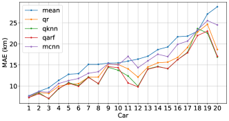
Figure 1: The MAE per vehicle when predicting driving distance. The cars are sorted by the MAE of the baseline (mean)

The prediction models’ performance when predicting the first departure time of each day is displayed in Table II. As in the driving distance case, all models achieve a lower MAE than the baseline, however, the improvement is rather slight. QR achieves the lowest MAE of 2.75 hours, which makes it on average around 30 min more accurate than the baseline. However, looking at the percentage of predicted departure times that are within an hour of the true departure time, it is clear that most of the prediction models are fairly more accurate than the baseline. The baseline only predicts 14% of the departure times within an hour of the actual departure, compared to 34% for the best performing prediction models. When looking at the MAPE, we can see a significant difference compared to the trip distance prediction. This makes sense when considering the nature of the predictions. In the departure time setting, it is reasonable to assume that a trip is performed a couple of hours into the day, which is considerably larger than the MAE displayed in Table II. In the distance setting, it is likely that the distance driven might be short. Depending on the actual driven distance, it may happen that the models predict double the distance, even if it is just a matter of a few kilometers.

TABLE II: Model performance when predicting departure time.

Model	MAE (hours)		MAPE		Percentage with error less than 60 min
	All	Best	All	Best	All	Best
Mean	3.22	2.21	82.89	24.72	14	22
QR	2.75	1.64	76.40	15.35	34	60
QKNN	2.94	1.97	72.47	18.41	34	63
QARF	2.90	1.93	71.02	19.14	32	64
FFNN	3.03	2.08	79.34	23.05	18	29

Figure 2 shows the MAE of each vehicle in the test set, giving a more extensive view of the models’ performances. As in the case of driving distance, the figure shows that the models’ accuracies differ considerably among vehicles. We may again note that the models produce significantly more accurate predictions than the baseline on some vehicles, while for other vehicles there are no accuracy improvements.

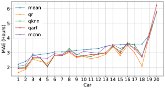
Figure 2: The MAE per vehicle when predicting departure time. The cars are sorted by the MAE of the baseline (mean)

The evaluation implies consistency across the two prediction targets in the models’ performances. The least accurate model in almost all cases is the baseline. FFNN slightly outperforms the baseline in most cases, but is less accurate than QR, QKNN, and QARF. QR performs well when predicting departure times, yielding the lowest MAE when considering all cars. However, QR does not perform as well when predicting driving distance and is less accurate than QKNN and QARF in this case. Figures 1 and 2 show that QKNN and QARF most often are among the top-performing models.

Figure 3 shows examples from a single vehicle of how MAE changes when the number of observations increases. We can note that it is not always the case that more observations yield a lower MAE. Periodically, the MAE might increase due to changing vehicle usage. For example we have noted that the summer period seems to often cause temporary changes in vehicle usage, resulting in increased prediction errors.

(a) Driving distance

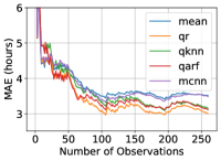
(b) Departure time

Figure 3: Examples from a single vehicle on how the MAE changes as more drives are observed when predicting driving distance and departure time.

From Figure 3 we can also note that all models, including the baseline, have similar curves and that the models’ MAE s seem to be affected in similar ways when observing new data. This suggests that all models are making quite similar predictions. One reason for this may be that no model manages to learn the full vehicle behavior, but rather they all learn some average or the most common drive.

VII-B Uncertainty

Table III displays how well the models estimate 90% prediction intervals for driving distances and departure times. Both tables show that the models generally do not reach the desired coverage probability, however, FFNN, QARF and QKNN all have coverage probabilities close to 90%. However, the MPIW is very large in all these cases, spanning tens of kilometers or several hours. QR produces much narrower intervals, but the PICP is significantly less than desired.

TABLE III: Model performance when creating prediction intervals

Model	Driving Distance		Departure Time
	PICP	MPIW	PICP	MPIW
QR	0.56	26.22	0.70	9.03
QKNN	0.81	61.45	0.83	10.83
QARF	0.84	79.83	0.85	11.37
MCNN	0.92	87.31	0.88	13.23

The results show that the prediction intervals are not perfectly accurate, as they often do not achieve the desired coverage probability. However, this is somewhat expected. As mentioned in Section VI, we begin measuring the PICP after the models have observed 20 drives. It is unlikely that the first 20 drives represent a vehicle’s full usage during a year, and the models may therefore not be expected to quantify the uncertainty perfectly yet. Instead, the models continue to improve as more drives are observed.

Figure 4 illustrates, for a single vehicle, how PICP and MPIW change as more observations are received. Both figures show how QKNN, QARF, and FFNN quickly reach a fairly high PICP, while QR needs many more observations to begin approaching a comparable prediction coverage. The pattern is similar in the case of MPIW. The prediction intervals of QKNN, QARF, and FFNN have a large width after only a few observations, while QR needs many more observations to reach a similar MPIW.

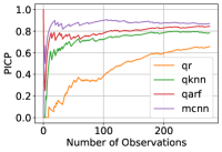
(a) PICP Driving distance

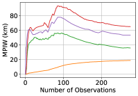
(b) MPIW Driving distance

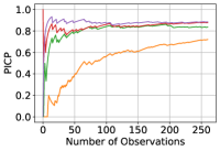
(c) PICP Departure time

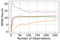
(d) MPIW Departure time

Figure 4: Examples from a single vehicle on how the PICP and MPIW change over time when predicting driving distance and departure time.

VIII Conclusion

In this study, we aim to predict the departure time and driving distance of the first drive of the day, using online learning models of different complexities. The prediction models are evaluated according to their error rate and how well they could estimate a 90% prediction interval. Based on this, we attempt to answer the question from Section III: How accurately can online learning models predict the departure time and distance of an upcoming drive?

When we look at all drives of all cars in the test set, the proposed prediction models generally yield an MAE of slightly below 3 hours when predicting departure time and 13-16 km when predicting driving distance. In the case of departure time, QR displays the best predictive performance while QARF and QKNN performs best in the driving distance case. The models’ ability to quantify uncertainty varies, with FFNN and QARF generally estimating the most accurate prediction intervals. The results indicate the surprising difficulty of predicting vehicle usage.

In the pre-pandemic period, it would be reasonable to assume better performance of the methods due to more stable commute patterns, see Section II. However, in the post-pandemic period, people are expected to commute less than before. Thus, while we expect an improvement as the new patterns stabilize, this improvement might not be major.

In this project, we use online learning since it fits well with the setting of the problem and potentially allows us to implement the models on the cars. Our prediction models yield similar error rates as the batch-learning models used in related work, even though our data was collected during the COVID-19 pandemic. Unfortunately, as the projects use different data sources, it is not possible to conclude if online models are as accurate. Thus, it would be interesting to compare online learning with batch learning in terms of MAE using the same data.

References

- [1] European Comission, “Delivering the European Green Deal,” [Online]. Available: https://ec.europa.eu/info/strategy/priorities-2019-2024/european-green-deal/delivering-european-green-deal\_en (last accessed on 2021-12-10).
- [2] Department for Business, Energy & Industrial Strategy and Department for Transport, “COP26 declaration on accelerating the transition to 100% zero emission cars and vans,” 2022, [Online]. Available: https://www.gov.uk/government/publications/cop26-declaration-zero-emission-cars-and-vans/cop26-declaration-on-accelerating-the-transition-to-100-zero-emission-cars-and-vans (last accessed on 2022-06-02).
- [3] Office of Governor Gavin Newsom, “Governor Newsom Announces California Will Phase Out Gasoline-Powered Cars & Drastically Reduce Demand for Fossil Fuel in California’s Fight Against Climate Change,” 2020, [Online]. Available: https://www.gov.ca.gov/2020/09/23/governor-newsom-announces-california-will-phase-out-gasoline-powered-cars-drastically-reduce-demand-for-fossil-fuel-in-californias-fight-against-climate-change/ (last accessed on 2022-06-02).
- [4] IEA, “Trends in electric light-duty vehicles,” 2022, [Online]. Available: https://www.iea.org/reports/global-ev-outlook-2022/trends-in-electric-light-duty-vehicles (last accessed on 2022-10-25).
- [5] D. Ramsey, A. Bouscayrol, and L. Boulon, “Energy consumption of a battery electric vehicle in winter considering preheating: Tradeoff between improved performance and total energy consumption,” IEEE Vehicular Technology Magazine, vol. 17, no. 3, pp. 104–112, 2022.
- [6] Y. Al-Wreikat, C. Serrano, and J. R. Sodré, “Effects of ambient temperature and trip characteristics on the energy consumption of an electric vehicle,” Energy, vol. 238, p. 122028, 2022.
- [7] V. Losing, B. Hammer, and H. Wersing, “Incremental on-line learning: A review and comparison of state of the art algorithms,” Neurocomputing, vol. 275, pp. 1261–1274, Jan 2018.
- [8] A. Gepperth and B. Hammer, “Incremental learning algorithms and applications,” in European Symposium on Artificial Neural Networks (ESANN), 2016.
- [9] D. Mukherjee and S. Datta, “Incremental time series algorithms for iot analytics: An example from autoregression,” in Proceedings of the 17th International Conference on Distributed Computing and Networking, ser. ICDCN ’16, 2016.
- [10] L. Cheng, D. Schuurmans, S. Wang, T. Caelli, and S. Vishwanathan, “implicit online learning with kernels,” in Advances in Neural Information Processing Systems, vol. 19. MIT Press, 2006.
- [11] O. Frendo, N. Gaertner, and H. Stuckenschmidt, “Improving smart charging prioritization by predicting electric vehicle departure time,” IEEE Transactions on Intelligent Transportation Systems, vol. 22, no. 10, pp. 6646–6653, 2021.
- [12] S. Baghali, S. Hasan, and Z. Guo, “Analyzing the travel and charging behavior of electric vehicles - a data-driven approach,” in 2021 IEEE Kansas Power and Energy Conference (KPEC), 2021, pp. 1–5.
- [13] B. Hilpisch, “Construction of a user-level probabilistic forecast of electric vehicle usage,” Semester Thesis, Institute of Cartography and Geoinformation, Swiss Federal Institute of Technology (ETH) Zurich, Zurich, Switzerland, 2020. doi: 10.3929/ethz-b-000460506.
- [14] C. Goebel and M. Voß, “Forecasting driving behavior to enable efficient grid integration of plug-in electric vehicles,” in 2012 IEEE Online Conference on Green Communications (GreenCom), 2012, pp. 74–79.
- [15] D. Panahi, S. Deilami, M. A. S. Masoum, and S. M. Islam, “Forecasting plug-in electric vehicles load profile using artificial neural networks,” in 2015 Australasian Universities Power Engineering Conference (AUPEC), 2015, pp. 1–6.
- [16] H. Jahangir, S. S. Gougheri, B. Vatandoust, M. A. Golkar, A. Ahmadian, and A. Hajizadeh, “Plug-in electric vehicle behavior modeling in energy market: A novel deep learning-based approach with clustering technique,” IEEE Transactions on Smart Grid, vol. 11, no. 6, pp. 4738–4748, 2020.
- [17] S. Shahriar and A. R. Al-Ali, “Impacts of covid-19 on electric vehicle charging behavior: Data analytics, visualization, and clustering,” Applied System Innovation, vol. 5, no. 1, 2022.
- [18] A. A. Nassar, K. Gandhi, and W. G. Morsi, “Electric vehicles load forecasting considering the effect of covid-19 pandemic,” in 2021 IEEE Electrical Power and Energy Conference (EPEC), 2021, pp. 440–444.
- [19] A. de Palma and S. Vosough, “Long, medium, and short-term effects of COVID-19 on mobility and lifestyle,” THEMA (THéorie Economique, Modélisation et Applications), Université de Cergy-Pontoise, THEMA Working Papers 2021-06, 2021.
- [20] A. de Palma, S. Vosough, and F. Liao, “An overview of effects of covid-19 on mobility and lifestyle: 18 months since the outbreak,” Transportation Research Part A: Policy and Practice, vol. 159, pp. 372–397, 2022.
- [21] L. W. Hiselius and P. Arnfalk, “When the impossible becomes possible: Covid-19’s impact on work and travel patterns in swedish public agencies,” European Transport Research Review, vol. 13, 2021.
- [22] Y. Gao and D. Levinson, “A bifurcation of the peak: new patterns of traffic peaking during the covid-19 era,” Transportation, pp. 1–21, 09 2022.
- [23] M. Javadinasr, T. Maggasy, M. Mohammadi, K. Mohammadain, E. Rahimi, D. Salon, M. W. Conway, R. Pendyala, and S. Derrible, “The long-term effects of covid-19 on travel behavior in the united states: A panel study on work from home, mode choice, online shopping, and air travel,” Transportation Research Part F: Traffic Psychology and Behaviour, vol. 90, pp. 466–484, 2022.
- [24] L. Calearo, M. Marinelli, and C. Ziras, “A review of data sources for electric vehicle integration studies,” Renewable and Sustainable Energy Reviews, vol. 151, p. 111518, 2021.
- [25] S. Shahriar, A. R. Al-Ali, A. H. Osman, S. Dhou, and M. Nijim, “Prediction of ev charging behavior using machine learning,” IEEE Access, vol. 9, pp. 111 576–111 586, 2021.
- [26] L. Zhu and N. Laptev, “Deep and confident prediction for time series at uber,” in 2017 IEEE International Conference on Data Mining Workshops (ICDMW). IEEE, 2017, pp. 103–110.
- [27] Q. Wang, Y. Ma, K. Zhao, and Y. Tian, “A comprehensive survey of loss functions in machine learning,” Annals of Data Science, vol. 9, no. 2, pp. 187–212, 2022.
- [28] R. Koenker and K. F. Hallock, “Quantile regression,” Journal of economic perspectives, vol. 15, no. 4, pp. 143–156, 2001.
- [29] T. Hastie, R. Tibshirani, and J. Friedman, The Elements of Statistical Learning: Data Mining, Inference, and Prediction. Springer, 2009.
- [30] S. P. Vasseur and J. L. Aznarte, “Comparing quantile regression methods for probabilistic forecasting of no2 pollution levels,” Scientific Reports, vol. 11, no. 1, pp. 1–8, 05 2021.
- [31] H. M. Gomes, A. Bifet, J. Read, J. P. Barddal, F. Enembreck, B. Pfharinger, G. Holmes, and T. Abdessalem, “Adaptive random forests for evolving data stream classification,” Machine Learning, vol. 106, 2017.
- [32] H. M. Gomes, J. P. Barddal, L. E. Boiko, and A. Bifet, “Adaptive random forests for data stream regression,” European Symposium on Artificial Neural Networks, Computational Intelligence and Machine Learning (ESANN), 2018.
- [33] P. Domingos and G. Hulten, “Mining high-speed data streams,” in Proceeding of the Sixth ACM SIGKDD International Conference on Knowledge Discovery and Data Mining, 2000.
- [34] E. Ikonomovska, J. Gama, and S. Džeroski, “Learning model trees from evolving data streams,” Data Mining and Knowledge Discovery, vol. 23, pp. 128–168, 07 2011.
- [35] D. Boulegane, A. Bifet, H. Elghazel, and G. Madhusudan, “Streaming time series forecasting using multi-target regression with dynamic ensemble selection,” in 2020 IEEE International Conference on Big Data (Big Data), 12 2020, pp. 2170–2179.
- [36] T. Vasiloudis, G. D. F. Morales, and H. Boström, “Quantifying uncertainty in online regression forests.” Journal of machine learning research, vol. 20, no. 155, pp. 1–35, 2019.
- [37] Y. Gal. Uncertainty in deep learning. Ph.D. dissertation, Department of Engineering University of Cambridge, 2016.
- [38] N. Tagasovska and D. Lopez-Paz, “Single-model uncertainties for deep learning,” Advances in Neural Information Processing Systems, vol. 32, 2019.
- [39] Y. Lai, Y. Shi, Y. Han, Y. Shao, M. Qi, and B. Li, “Exploring uncertainty in regression neural networks for construction of prediction intervals,” Neurocomputing, vol. 481, pp. 249–257, 2022.
- [40] Y. Kwon, J.-H. Won, B. J. Kim, and M. C. Paik, “Uncertainty quantification using bayesian neural networks in classification: Application to biomedical image segmentation,” Computational Statistics & Data Analysis, vol. 142, p. 106816, 2020.
- [41] M. H. Shaker and E. Hüllermeier, “Aleatoric and epistemic uncertainty with random forests,” in Advances in Intelligent Data Analysis XVIII, 2020, pp. 444–456.
- [42] Y. Gal and Z. Ghahramani, “Dropout as a bayesian approximation: Representing model uncertainty in deep learning,” in Proceedings of The 33rd International Conference on Machine Learning, M. F. Balcan and K. Q. Weinberger, Eds., vol. 48, 2016, pp. 1050–1059.
- [43] H. M. Gomes, J. Read, A. Bifet, J. P. Barddal, and J. a. Gama, “Machine learning for streaming data: State of the art, challenges, and opportunities,” ACM SIGKDD Explorations Newsletter, vol. 21, no. 2, p. 6–22, nov 2019.
- [44] G. Cross and A. Jain, “Measurment of clustering tendency,” in Theory and Application of Digital Control. Pergamon, 1982, pp. 315–320.
- [45] A. Bhandari. What is Multicollinearity? Here’s Everything You Need to Know . Analytics Vidhya.
- [46] A. Blum, A. Kalai, and J. Langford, “Beating the hold-out: Bounds for k-fold and progressive cross-validation,” in Proceedings of the Twelfth Annual Conference on Computational Learning Theory (COLT), 1999, p. 203–208.
- [47] R. Ghawi and J. Pfeffer, “Efficient hyperparameter tuning with grid search for text categorization using knn approach with bm25 similarity,” Open Computer Science, vol. 9, no. 1, pp. 160–180, 2019.
- [48] T. Lindroth and A. Svensson. (2022) Predicting vehicle usage using incremental machine learning. M.Sc. thesis, Department of Computer Science and Engineering, Chalmers University of Technology.