Evaluating the Impact of Loss Function Variation in Deep Learning for Classification

Abstract

The loss function is arguably among the most important hyperparameters for a neural network. Many loss functions have been designed to date, making a correct choice nontrivial. However, elaborate justifications regarding the choice of the loss function are not made in related work. This is, as we see it, an indication of a dogmatic mindset in the deep learning community which lacks empirical foundation. In this work, we consider deep neural networks in a supervised classification setting and analyze the impact the choice of loss function has onto the training result. While certain loss functions perform suboptimally, our work empirically shows that under-represented losses such as the KL Divergence can outperform the State-of-the-Art choices significantly, highlighting the need to include the loss function as a tuned hyperparameter rather than a fixed choice.

1 Introduction

In recent years, Deep Neural Networks (DNNs) such as Convolutional Neural Networks (CNNs; [LeCun et al. (1989)]) have been used extensively for learning tasks, including classification. In a supervised setting, neural networks vitally require an understanding of goodness of their prediction which they receive via the loss function. Many loss functions have been proposed so far, some of which are tailored to specific problems [Wang et al. (2019), Diakogiannis et al. (2020), Demirkaya et al. (2020), Feng et al. (2018), Lin et al. (2017)] while we can more generally distinguish between loss functions for classification and loss functions for regression [Muthukumar et al. (2021)]. In this work, we are only concerned with the classification case.

Usually, researchers select a loss function and assume it throughout their publication. We highlight the use of seemingly axiomatic statements such as “We adopt Mean-Square Error (MSE) as the loss function [ …], who [sic] could be rather sensitive to outliers.” [Wang et al. (2016)], “The Cross Entropy is used as loss function [ …]” [Tabik et al. (2017)] and “For parameter optimization, we use the Adam optimizer with cross-entropy loss function.” [An et al. (2020)]. Some work [Chauhan et al. (2018), Ciresan et al. (2011)] is cited hundred- and thousand-fold but does not mention which loss measure was used.

The loss measure arguably does not receive extensive attention with regards to optimization in deep learning research but is rather subject to a dogmatic choice. We opine however, that this dogmatic mindset is misplaced in deep learning due to it being deeply ingrained into the learning process [Yessou et al. (2020)] Thus, we conjecture that a poor choice of loss measure leads to converse effects like a bad loss surface, local optima and stalled or slowed optimization. This can in turn lead to an increase in required epochs and model complexity which pose a higher computational demand on the computing infrastructure. In this analysis, we vary the loss function across our experiments in order to explore the impact this has on the training outcome.

2 Considered Loss Functions

Consider the scenario of classifying data points from a data set $\mathcal{D}=\{(x_{i},y_{i})\}_{i=1}^{N}$ into $c\in\mathbb{N}$ classes. Using a neural network, a function $f_{\theta}$ that maps each data point onto its corresponding class is learned over a set of weights $\theta$. To do so, the predicted output and its class are compared by a loss function $\mathcal{L}$ which indicates how good the prediction was. Subsequently, the loss function is derived wrt. $\theta$ in order to move $\theta$ into the direction of steepest descent [Rumelhart et al. (1985)]. Formally, we are interested in

$$\operatorname*{arg\,min}_{\theta\,\in\,\Theta}\ \operatorname*{\mathbb{E}}_{x,y}\quantity[\mathcal{L}(f_{\theta}(x),y)].$$

However, we do not know the data’s joint distribution $P(\mathcal{X},\mathcal{Y})$ and thus have to resort to the expected value’s empirical formulation

$$\operatorname*{arg\,min}_{\theta\,\in\,\Theta}\ \frac{1}{N}\sum\limits_{i=1}^{N}\mathcal{L}(f_{\theta}(x_{i}),y_{i}).$$

In this work, we consider each label $y_{i}$ to be one-hot encoded and thus assume that $f_{\theta}(x_{i})\in\mathbb{R}^{c}$ returns a vector of probabilities corresponding to the model’s confidence in each class which can be achieved via the Softmax function.

Our analysis incorporates four loss functions (listed in Table 1) that have been widely used in machine learning. Intuitively, these have different properties, for example, the MAE is Lipschitz continuous with Lipschitz constant $L=1$ [Qi et al. (2020)]. Besides that, it inherits the absolute value function’s discontinuity at 0. Because the MSE squares its arguments component-wise, large differences in the components lead to outliers being penalized stronger. The MAE, on the other hand, is insensitive to outliers because it weighs all data points equally [Chai and Draxler (2014)]. The CCE’s gradients tend to be steep which is conjectured to be a reason it converges quickly [Bosman et al. (2020)]. Both CCE and KLD are not symmetric whereas the MSE and MAE are. The CCE and KLD have information theoretic interpretations: according to Murphy (2012), the CCE is the mean number of bits required to encode a source distribution (label distribution) using a model distribution (prediction distribution). Furthermore, the KLD decomposes into

$$\mathcal{L}_{\mathrm{KLD}}(\hat{y},y)=\mathcal{L}_{\mathrm{CCE}}(\hat{y},y)-\mathbb{H}(y)$$ (1)

with $\mathbb{H}(\cdot)$ being the entropy Murphy (2012). Therefore, the KLD is the mean number of additional bits required to encode the data.

Table 1: Loss functions used in this work. Models using these are implemented, trained and evaluated in the Experiments section.

Loss Function	Abbreviation	Expression
Mean Square Error Bickel and Doksum (2015)	MSE	$\sum\limits_{k=1}^{c}\left(\hat{y}^{(k)}-y^{(k)}\right)^{2}$
Mean Absolute Error Ghosh et al. (2017)	MAE	$\sum\limits_{k=1}^{c}\absolutevalue{\hat{y}^{(k)}-y^{(k)}}$
(Categorical) Cross-Entropy Murphy (2012)	(C)CE	$\sum\limits_{k=1}^{c}-y^{(k)}\log\left(\hat{y}^{(k)}\right)$
Kullback-Leibler Divergence Kullback and Leibler (1951)	KLD	$\sum\limits_{k=1}^{c}y^{(k)}\log\left(\frac{y^{(k)}}{\hat{y}^{(k)}}\right)$

3 Related Work

Similar to our work, Janocha and Czarnecki (2017) compared 12 loss functions in a classification regime. They investigated synthetic data as well as MNIST LeCun et al. (1989). The experimental results obtained by Janocha and Czarnecki (2017) and Demirkaya et al. (2020) yielded intriguing insight into loss functions for sufficiently complex data sets: less common, non-classical losses such as the Tanimoto loss Diakogiannis et al. (2020) and the Correct-Class Quadratic Loss (CCQL; Demirkaya et al. (2020)) achieved very good performances. In an effort to improve the MAE, Wang et al. (2019) proposed the Improved Mean Absolute Error (IMAE) which, compared to the MAE, led to an increase in training accuracy by 18.8 % on CIFAR-10.

Despite the success in employing the IMAE, Tanimoto loss and CCQL, we focus on the most popular loss functions which is why less popular (but well-performing) functions are not incorporated in our analysis. However, we applied our analysis onto more datasets to measure a more generalized impact.

4 Experiments

In this section, we present an array of experiments regarding the loss functions from Table 1. In order to avoid results occurring by stochasticity, we generate 6 outcomes (iterations) for each combination of data set and loss function and compute the respective mean metrics. Figure 1 shows a conceptual diagram of our approach. Training took place using 2 $\times$ NVIDIA RTX 8000 + 12 $\times$ Intel Xeon + 32 GB RAM. All models are trained for 100 epochs using the Adam optimizer Kingma and Ba (2014).

Figure 1: Our experiments as a network diagram.

Data Sets.

We used six data sets as presented in Table 2, three of which are popular benchmarking data sets. The other three (Mushroom, Phishing and CharFontIm) are known to a lesser extent. Mushroom and Phishing are tabular data sets. We performed feature analysis via PCA Abdi and Williams (2010) and concluded that for Mushroom, nearly 100 % of the data’s variance can be explained by 15 features. Thus, we reduced Mushroom to its 15 most important features, which are, by index: 0, 1, 3, 6, 7, 8, 10, 11, 13, 14, 16, 17, 18, 19, 20.

Table 2: Summary of our data sets, including the train/validation/test split. The column PCA indicates whether any feature reduction via PCA took place; a squiggly arrow in the Features column indicates the reduction result. The Train Split column gives the percentages of the resulting split into train/validation/test set, respectively.

Data Set	$N$	$c$	Features	PCA	Batch Size	Train Split (%)
Mushroom Dua and Graff (2017)	8,124	2	22 $\rightsquigarrow$ 15		16	50 / 10 / 40
Phishing Dua and Graff (2017)	11,055	2	29		16	50 / 10 / 40
MNIST LeCun et al. (1989)	70,000	10	$28\times 28$		64	76 / 10 / 14
Fashion-MNIST Xiao et al. (2017)	70,000	10	$28\times 28$		64	76 / 10 / 14
CIFAR-10 Krizhevsky and Hinton (2009)	60,000	10	$32\times 32\times 3$		64	74 / 10 / 16
CharFontIm Dua and Graff (2017)	745,000	153	$20\times 20$		128	60 / 10 / 30

Hyperparameters.

We perform a broad hyperparameter search across the learning rate ($\lambda$) and $\ell_{2}$ weight decay ($\eta$). The model for each combination is trained for 20 epochs. Consequently, we choose the parameters that led to the highest validation accuracy. In total, we sample 30 candidates for $\lambda$ and $\eta$ from the log-uniform distribution over $[$110-5$,$110-1$]$.

Table 3: Hyperparameter configuration for each model and loss function. We round each parameter to the nearest most significant digit. $\lambda^{\ast}$ and $\eta^{\ast}$ denote the best learning rate and weight decay coefficient, respectively.

	MSE		MAE		CCE		KLD
Data Set	$\lambda^{\ast}$	$\eta^{\ast}$	$\lambda^{\ast}$	$\eta^{\ast}$	$\lambda^{\ast}$	$\eta^{\ast}$	$\lambda^{\ast}$	$\eta^{\ast}$
Mushroom	$310-3$	$210-3$	$310-3$	$110-4$	$910-4$	$210-5$	$510-4$	$910-4$
Phishing	$710-5$	$410-5$	$110-5$	$210-5$	$310-5$	$110-5$	$710-4$	$410-3$
MNIST	$210-3$	$110-5$	$210-4$	$310-5$	$110-5$	$910-5$	$510-4$	$410-3$
Fashion-MNIST	$510-4$	$210-4$	$110-5$	$210-5$	$610-5$	$310-3$	$610-4$	$210-4$
CIFAR-10	$110-2$	$210-5$	$510-2$	$110-2$	$210-4$	$210-3$	$310-5$	$310-5$
CharFontIm	$210-5$	$310-3$	$910-3$	$310-2$	$410-5$	$110-3$	$110-4$	$410-5$

Architectures.

Two convolutional architectures are obtained from related work Chauhan et al. (2018); Çalik and Demirci (2018) while the one used on CharFontIm is our own. We chose these because they performed reasonably well on CIFAR-10 and MNIST (80.17 % and 99.6 % training accuracy, respectively). We use a Multi-Layer Perceptron (MLP) architecture for the tabular data sets, inspired by previous work on categorical classifiers Vashisth et al. (2020); Potghan et al. (2018); Desai and Shah (2021); Wan et al. (2018); Yulita et al. (2018); Das et al. (2018). For visualizations of the CNNs/MLP, we refer to Appendix A.

Evaluation Metrics.

We use three metrics in order to assess the trained classifiers’ performances. (I) Test accuracy: we observe the progression of accuracy per elapsed epoch. The final attained test accuracy is compared across all loss functions. (II) Matthew’s Correlation Coefficient ($\phi$) Yule (1912); Matthews (1975). (III) Area Under Curve (AUC) Collinson (1998).

Results.

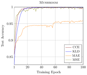
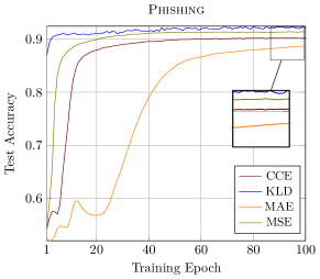
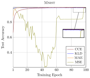
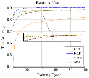
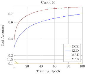
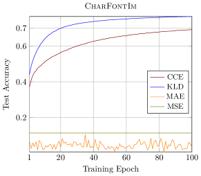
Figure 4: Test accuracies on each data set (across 6 iterations). Points of interest are inset.

Table 4 shows the mean test accuracies across $M=6$ iterations of an experiment. In Table 5, we present the attained mean performances for $\phi$ and AUC. Our results show that, performance-wise, the KLD outperforms all other loss functions in 4 out of 6 experiments. Remarkably, the KLD attains 100 % test accuracy on all 6 iterations for Mushroom. While the State-of-the-Art for classification (CCE) performs slightly worse than the MSE, it is more stable. Unexpectedly, the MAE performs best and most stably on MNIST solely. However, as we transition to more challenging data sets, test accuracy degrades into pathological cases for the MSE and MAE; on CIFAR-10, they were only able to ever predict one class (10 % accuracy). During training, the MAE almost always kept an offset in test accuracy to the other losses (cf. Figure 4 in Appendix B). We hypothesize that this is due to its bad gradient properties. On MNIST, its performance was best which we attribute to the possibility that MNIST may be classifiable by learning its conditional median $\operatorname*{\mathbb{E}}\quantity[\absolutevalue{f_{\theta}(x)-y_{i}}\mid x=x_{i}]$, $i\in\{1,\dots,N\}$.

Table 4: Mean attained test accuracies and corresponding standard error of mean (SEM) after 100 epochs. The best accuracies $\pm$ SEMs for each row are boldfaced. A higher mean accuracy is better. A lower SE is better except if the attained accuracy is pathological. Here, the SE should be understood as a measure of stability across $M$ iterations of an experiment.

Data Set	MSE			MAE			CCE			KLD
Mushroom	$99.69\%$	$\pm$	$0.26\%$	$95.83\%$	$\pm$	$0.27\%$	$99.67\%$	$\pm$	$0.10\%$	$\mathbf{100.00}\%$	$\pm$	$\mathbf{0.00}\%$
Phishing	$91.41\%$	$\pm$	$\mathbf{0.08}\%$	$88.70\%$	$\pm$	$0.32\%$	$90.29\%$	$\pm$	$0.11\%$	$\mathbf{92.07}\%$	$\pm$	$0.26\%$
MNIST	$98.53\%$	$\pm$	$0.17\%$	$\mathbf{99.30}\%$	$\pm$	$\mathbf{0.01}\%$	$98.99\%$	$\pm$	$0.03\%$	$98.84\%$	$\pm$	$0.04\%$
Fashion-MNIST	$87.96\%$	$\pm$	$\mathbf{0.04}\%$	$82.04\%$	$\pm$	$0.09\%$	$88.60\%$	$\pm$	$0.11\%$	$\mathbf{90.47}\%$	$\pm$	$0.11\%$
CIFAR-10	$10.00\%$	$\pm$	$0.00\%$	$10.00\%$	$\pm$	$0.00\%$	$\mathbf{78.13}\%$	$\pm$	$\mathbf{0.28}\%$	$70.05\%$	$\pm$	$0.30\%$
CharFontIm	$11.30\%$	$\pm$	$0.00\%$	$3.37\%$	$\pm$	$1.52\%$	$69.21\%$	$\pm$	$0.97\%$	$\mathbf{76.62}\%$	$\pm$	$\mathbf{0.02}\%$

Table 5: Performance metrics for the data sets. The best entries for each row are boldfaced. Recall that a higher $\phi$ and a higher AUC is better. For MNIST, no AUC column is boldfaced since all attain equal values. For pathological cases (MSE/MAE for CIFAR-10 and CharFontIm), no entry is boldfaced.

MSE MAE CCE KLD Data Set $\phi$ AUC $\phi$ AUC $\phi$ AUC $\phi$ AUC Mushroom 0.99 0.99 0.91 0.94 0.99 1.00 $\mathbf{1.00}$ $\mathbf{1.00}$ Phishing 0.82 0.96 0.77 0.94 0.80 0.96 $\mathbf{0.83}$ $\mathbf{0.97}$ MNIST 0.98 0.99 $\mathbf{0.99}$ 0.99 0.98 0.99 0.98 0.99 Fashion-MNIST 0.86 0.98 0.80 0.97 0.87 $\mathbf{0.99}$ $\mathbf{0.89}$ $\mathbf{0.99}$ CIFAR-10 0.00 0.50 0.00 0.50 $\mathbf{0.75}$ $\mathbf{0.97}$ 0.66 0.95 CharFontIm 0.00 0.50 0.00 0.50 0.67 0.98 $\mathbf{0.75}$ $\mathbf{0.99}$

5 Future Work

Our work leaves improvements for future research. Firstly, we believe that more data sets need to be incorporated into loss function variation analysis.

Secondly, since we only considered classification, our work leaves open the question of how the impact of loss function variation expresses in regression settings. How significant and nontrivial is the selection of the loss function in regression? Besides our restriction to four loss functions, we mentioned novel losses such as the IMAE, Tanimoto loss and CCQL which outperformed classical losses. Therefore, we recommend more work be dedicated to designing custom loss measures. A hypothesis regarding the KLD’s very good performance may be that the class of $f$-divergences provides good loss functions. Examples of $f$-divergences are the KLD, the Bhattacharyya divergence Bhattacharyya (1943) and Hellinger distance Hellinger (1909).

Thirdly, an expansion to sequence-based models would be interesting. To date, several well-performing neural architectures, such as the Transformer Vaswani et al. (2017), have been proposed.

6 Conclusions

In this work, we explored the impact of varying the loss function in different deep learning architectures on the training process and its performance. We considered the case of classifying data points into $c$ classes using probabilistic predictions with one-hot encoded labels. We have demonstrated empirically that on MNIST, the MAE can achieve a better classifier performance than the CCE or KLD. Our designation is that if rapid convergence is needed, the MSE can be favored for a low amount of classes. Our main finding is that the KLD outperforms the CCE on 4 out of 6 data sets. Along with very good test accuracies, two performance metrics are underpinnings of this result. Thus, our recommendation is to increase the KLD’s usage in binary and multi-class classification regimes. Due to its very bad performance on color images and overall subpar performance, we advise that using the MAE in a classification setting should be considered carefully. Finally, we encourage a paradigm shift that steers away from axiomatically fixating loss functions but considers them part of hyperparameter optimization.

Acknowledgements.

Computational infrastructure and support were provided by the Center for Information and Media Technology at Heinrich Heine University Düsseldorf.

Appendix A Architectures

[CNN architecture for MNIST. Dropout is applied after the 1 and 2 conv layer ($p=0.2$), as well as after the dense layer ($p=0.2$). The 1 conv layer has $5\times 5$ filters.]

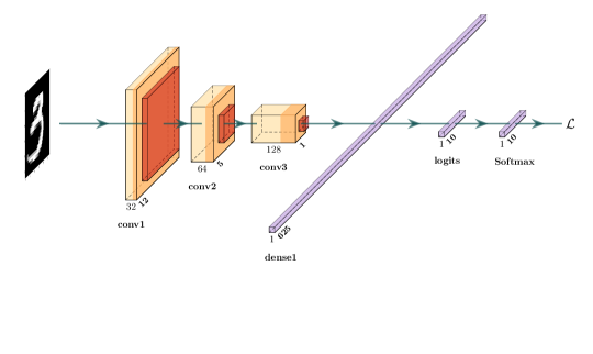
[CNN architecture for CIFAR-10. Dropout is applied after both Max-Pool layers ($p=0.25$), after the 4 conv layer ($p=0.25$) and after the dense layer ($p=0.5$). The 1 and 2 conv layer have $5\times 5$ filters.]

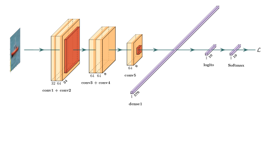
[CNN architecture for CharFontIm. Dropout is applied after the 2, 3 and 4 conv layer ($p=0.25$), as well as after the 1 and 2 dense layers ($p=0.5$). Filters have size $5\times 5$ for the 1 and 2 conv layers.]

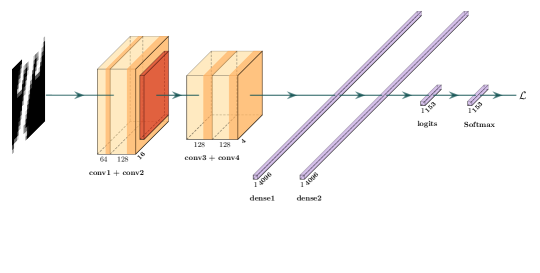
Figure 2: CNN architectures. Red layers are Max-Pool layers of size $2\times 2$. If not specified, the filter size of a conv layer is $3\times 3$.

Figure 3: Our dense architecture. Hidden layers have a teal color. The first dense layer has 32 neurons, the second and third 64, and the fourth 32. This is followed by a fifth dense layer (red-ish colored) having 2 output neurons. Dropout is applied after the first 3 hidden layers ($p=0.4\rightarrow 0.2\rightarrow 0.2$). Note that this representation is not confined to a fixed number of classes or neurons; the vertical dots indicate that it is indeed conceptual.

Appendix B Accuracy Progressions

References

- Abdi and Williams (2010) Hervé Abdi and Lynne J. Williams. Principal component analysis. WIREs Computational Statistics, 2(4):433–459, 2010. https://doi.org/10.1002/wics.101.
- An et al. (2020) Sanghyeon An, Minjun Lee, Sanglee Park, Heerin Yang, and Jungmin So. An ensemble of simple convolutional neural network models for MNIST digit recognition. arXiv preprint arXiv:2008.10400, 2020.
- Bhattacharyya (1943) Anil Bhattacharyya. On a measure of divergence between two statistical populations defined by their probability distributions. Bull. Calcutta Math. Soc., 35:99–109, 1943.
- Bickel and Doksum (2015) Peter J. Bickel and Kjell A. Doksum. Mathematical Statistics: Basic Ideas and Selected Topics, Volumes I–II Package. Chapman and Hall/CRC, 2015.
- Bosman et al. (2020) Anna Sergeevna Bosman, Andries Engelbrecht, and Mardé Helbig. Visualising basins of attraction for the cross-entropy and the squared error neural network loss functions. Neurocomputing, 400:113–136, 2020.
- Çalik and Demirci (2018) Rasim Caner Çalik and M. Fatih Demirci. Cifar-10 image classification with convolutional neural networks for embedded systems. In 2018 IEEE/ACS 15th International Conference on Computer Systems and Applications (AICCSA), pages 1–2. IEEE, 2018.
- Chai and Draxler (2014) Tianfeng Chai and Roland R. Draxler. Root mean square error (RMSE) or mean absolute error (MAE)? – arguments against avoiding RMSE in the literature. Geoscientific Model Development, 7(3):1247–1250, 2014.
- Chauhan et al. (2018) Rahul Chauhan, Kamal Kumar Ghanshala, and R. C. Joshi. Convolutional neural network (CNN) for image detection and recognition. In 2018 First International Conference on Secure Cyber Computing and Communication (ICSCCC), pages 278–282. IEEE, 2018.
- Ciresan et al. (2011) Dan Claudiu Ciresan, Ueli Meier, Jonathan Masci, Luca Maria Gambardella, and Jürgen Schmidhuber. Flexible, high performance convolutional neural networks for image classification. In Twenty-Second International Joint Conference on Artificial Intelligence, 2011.
- Collinson (1998) P. Collinson. Of bombers, radiologists, and cardiologists: time to ROC. Heart, 80(3):215–217, 1998.
- Das et al. (2018) Anup Das, Francky Catthoor, and Siebren Schaafsma. Heartbeat classification in wearables using multi-layer perceptron and time-frequency joint distribution of ECG. In Proceedings of the 2018 IEEE/ACM International Conference on Connected Health: Applications, Systems and Engineering Technologies, pages 69–74, 2018.
- Demirkaya et al. (2020) Ahmet Demirkaya, Jiasi Chen, and Samet Oymak. Exploring the role of loss functions in multiclass classification. In 2020 54th Annual Conference on Information Sciences and Systems (CISS), pages 1–5. IEEE, 2020.
- Desai and Shah (2021) Meha Desai and Manan Shah. An anatomization on breast cancer detection and diagnosis employing multi-layer perceptron neural network (MLP) and convolutional neural network (CNN). Clinical eHealth, 4:1–11, 2021.
- Diakogiannis et al. (2020) Foivos I. Diakogiannis, François Waldner, Peter Caccetta, and Chen Wu. ResUNet-a: A deep learning framework for semantic segmentation of remotely sensed data. ISPRS Journal of Photogrammetry and Remote Sensing, 162:94–114, 2020.
- Dua and Graff (2017) Dheeru Dua and Casey Graff. UCI machine learning repository, 2017. URL http://archive.ics.uci.edu/ml.
- Feng et al. (2018) Zhen-Hua Feng, Josef Kittler, Muhammad Awais, Patrik Huber, and Xiao-Jun Wu. Wing loss for robust facial landmark localisation with convolutional neural networks. In Proceedings of the IEEE Conference on Computer Vision and Pattern Recognition, pages 2235–2245, 2018.
- Ghosh et al. (2017) Aritra Ghosh, Himanshu Kumar, and PS Sastry. Robust loss functions under label noise for deep neural networks. In Proceedings of the AAAI Conference on Artificial Intelligence, volume 31, 2017.
- Hellinger (1909) Ernst Hellinger. Neue begründung der theorie quadratischer formen von unendlichvielen veränderlichen. Journal für die reine und angewandte Mathematik, 1909(136):210–271, 1909.
- Janocha and Czarnecki (2017) Katarzyna Janocha and Wojciech Marian Czarnecki. On loss functions for deep neural networks in classification. arXiv preprint arXiv:1702.05659, 2017.
- Kingma and Ba (2014) Diederik P. Kingma and Jimmy Ba. Adam: A method for stochastic optimization. arXiv preprint arXiv:1412.6980, 2014.
- Krizhevsky and Hinton (2009) Alex Krizhevsky and Geoffrey Hinton. Learning multiple layers of features from tiny images. 2009.
- Kullback and Leibler (1951) Solomon Kullback and Richard A. Leibler. On information and sufficiency. The Annals of Mathematical Statistics, 22(1):79–86, 1951.
- LeCun et al. (1989) Yann LeCun, Bernhard Boser, John S. Denker, Donnie Henderson, Richard E. Howard, Wayne Hubbard, and Lawrence D. Jackel. Backpropagation applied to handwritten zip code recognition. Neural Computation, 1(4):541–551, 1989.
- Lin et al. (2017) Tsung-Yi Lin, Priya Goyal, Ross Girshick, Kaiming He, and Piotr Dollár. Focal loss for dense object detection. In Proceedings of the IEEE International Conference on Computer Vision, pages 2980–2988, 2017.
- Matthews (1975) Brian W. Matthews. Comparison of the predicted and observed secondary structure of t4 phage lysozyme. Biochimica et Biophysica Acta (BBA)-Protein Structure, 405(2):442–451, 1975.
- Murphy (2012) Kevin P. Murphy. Machine Learning: A Probabilistic Perspective. MIT Press, 2012.
- Muthukumar et al. (2021) Vidya Muthukumar, Adhyyan Narang, Vignesh Subramanian, Mikhail Belkin, Daniel J. Hsu, and Anant Sahai. Classification vs regression in overparameterized regimes: Does the loss function matter? Journal of Machine Learning Research, 22:222:1–222:69, 2021.
- Potghan et al. (2018) Sneha Potghan, R. Rajamenakshi, and Archana Bhise. Multi-layer perceptron based lung tumor classification. In 2018 Second International Conference on Electronics, Communication and Aerospace Technology (ICECA), pages 499–502. IEEE, 2018.
- Qi et al. (2020) Jun Qi, Jun Du, Sabato Marco Siniscalchi, Xiaoli Ma, and Chin-Hui Lee. On mean absolute error for deep neural network based vector-to-vector regression. IEEE Signal Processing Letters, 27:1485–1489, 2020.
- Rumelhart et al. (1985) David E. Rumelhart, Geoffrey E. Hinton, and Ronald J. Williams. Learning internal representations by error propagation. Technical report, University of California San Diego, La Jolla Institute for Cognitive Science, 1985.
- Tabik et al. (2017) Siham Tabik, Daniel Peralta, Andres Herrera-Poyatos, and Francisco Herrera Triguero. A snapshot of image pre-processing for convolutional neural networks: case study of MNIST. 2017.
- Vashisth et al. (2020) Shubham Vashisth, Ishika Dhall, and Shipra Saraswat. Chronic kidney disease (CKD) diagnosis using multi-layer perceptron classifier. In 2020 10th International Conference on Cloud Computing, Data Science & Engineering (Confluence), pages 346–350. IEEE, 2020.
- Vaswani et al. (2017) Ashish Vaswani, Noam Shazeer, Niki Parmar, Jakob Uszkoreit, Llion Jones, Aidan N. Gomez, Łukasz Kaiser, and Illia Polosukhin. Attention is all you need. Advances in Neural Information Processing Systems, 30, 2017.
- Wan et al. (2018) Shaohua Wan, Yan Liang, Yin Zhang, and Mohsen Guizani. Deep multi-layer perceptron classifier for behavior analysis to estimate parkinson’s disease severity using smartphones. IEEE Access, 6:36825–36833, 2018.
- Wang et al. (2019) Xinshao Wang, Yang Hua, Elyor Kodirov, and Neil M. Robertson. IMAE for noise-robust learning: Mean absolute error does not treat examples equally and gradient magnitude’s variance matters. arXiv preprint arXiv:1903.12141, 2019.
- Wang et al. (2016) Zhangyang Wang, Shiyu Chang, Yingzhen Yang, Ding Liu, and Thomas S. Huang. Studying very low resolution recognition using deep networks. In Proceedings of the IEEE Conference on Computer Vision and Pattern Recognition, pages 4792–4800, 2016.
- Xiao et al. (2017) Han Xiao, Kashif Rasul, and Roland Vollgraf. Fashion-MNIST: a novel image dataset for benchmarking machine learning algorithms. arXiv preprint arXiv:1708.07747, 2017.
- Yessou et al. (2020) Hichame Yessou, Gencer Sumbul, and Begüm Demir. A comparative study of deep learning loss functions for multi-label remote sensing image classification. In IGARSS 2020-2020 IEEE International Geoscience and Remote Sensing Symposium, pages 1349–1352. IEEE, 2020.
- Yule (1912) G. Udny Yule. On the methods of measuring association between two attributes. Journal of the Royal Statistical Society, 75(6):579–652, 1912.
- Yulita et al. (2018) Intan Nurma Yulita, Rudi Rosadi, Sri Purwani, and Mira Suryani. Multi-layer perceptron for sleep stage classification. In Journal of Physics: Conference Series, volume 1028, page 012212. IOP Publishing, 2018.