Improving abstractive summarization with energy-based re-ranking

Abstract

Current abstractive summarization systems present important weaknesses which prevent their deployment in real-world applications, such as the omission of relevant information and the generation of factual inconsistencies (also known as hallucinations). At the same time, automatic evaluation metrics such as CTC scores Deng et al. (2021) have been recently proposed that exhibit a higher correlation with human judgments than traditional lexical-overlap metrics such as ROUGE. In this work, we intend to close the loop by leveraging the recent advances in summarization metrics to create quality-aware abstractive summarizers. Namely, we propose an energy-based model that learns to re-rank summaries according to one or a combination of these metrics. We experiment using several metrics to train our energy-based re-ranker and show that it consistently improves the scores achieved by the predicted summaries. Nonetheless, human evaluation results show that the re-ranking approach should be used with care for highly abstractive summaries, as the available metrics are not yet sufficiently reliable for this purpose.

1 Introduction

In recent years, abstractive methods have greatly benefited from the development and widespread availability of large-scale transformer-based language generative models Vaswani et al. (2017); Lewis et al. (2020); Raffel et al. (2020); Zhang et al. (2020), which are capable of generating text with unprecedented fluency. Despite the recent progress, abstractive summarization systems still suffer from problems that hamper their deployment in real-world applications. Omitting the most relevant information from the source document is one of such problems. Additionally, factual inconsistencies (also known as hallucinations) were estimated to be present in around 30% of the summaries produced by abstractive systems on the CNN/DailyMail dataset Kryscinski et al. (2019). This observation has motivated a considerable amount of research on strategies to mitigate the hallucination problem Falke et al. (2019); Cao et al. (2020); Zhao et al. (2020); Zhu et al. (2021), but the improvements achieved so far are mild. This is partly due to the difficulty of evaluating the quality of summaries automatically, leading to the adoption of metrics that are often insufficient or even inappropriate. Despite its limitations, ROUGE Lin (2004) is still the de facto evaluation metric for summarization, mostly due to its simplicity and interpretability. However, not only does it correlate poorly with human-assessed summary quality Kané et al. (2019), but it is also unreliable whenever the reference summary contains hallucinations, which unfortunately is not an uncommon issue in widely adopted summarization datasets Kryscinski et al. (2019); Maynez et al. (2020). For these reasons, the development of more reliable evaluation metrics with a stronger correlation with human judgment is also an active area of research Kryscinski et al. (2020); Scialom et al. (2021); Deng et al. (2021).

In this work, we propose a new approach to abstractive summarization via an energy-based model. In contrast to previous approaches, which use reinforcement learning to train models to maximize ROUGE or BERT scores Paulus et al. (2018); Li et al. (2019), our EBM is trained to re-rank the candidate summaries the same way that the chosen metric would rank them – a much simpler problem which is computationally much more efficient. This way, we are distilling the metric, which presents as a by-product an additional advantage: a quality estimation system that can be used to assess the quality of the summaries on the fly without the need of reference summaries. It should be remarked that any reference-free metric, can be used at inference time for re-ranking candidates from any abstractive summarization system, hence improving the quality of the generated summaries. Our re-ranking model can therefore leverage the advantages of recently proposed evaluation metrics over traditional ones, which are essentially two-fold: i) being able to better capture high-level semantic concepts, and ii) in addition to the target summary, these metrics take into account the information present on the source document, which is crucial to detect hallucinations. We demonstrate the effectiveness of our approach on standard benchmark datasets for abstractive summarization (CNN/DailyMail, Hermann et al. (2015), and XSum, Narayan et al. (2018)) and use a variety of summarization metrics as the target to train our model on, showing the versatility of the method. We also conduct a human evaluation experiment, in which we compare our re-ranking model trained to maximize recent transformer-based metrics that aim to measure factual consistency and relevance (CTC scores, Deng et al. (2021)). Our proposed model yields improvements over the usual beam search on a baseline model and demonstrates the ability to distill target metrics. However, the human evaluation results suggest that re-ranking according to these metrics, while competitive, may yield lower quality summaries than those obtained by state-of-the-art abstractive systems trained with augmented data and contrastive learning.

The remainder of the paper is organized as follows: in Section 2, we discuss the related work; in Section 3, we do a brief high-level description of neural abstractive summarization systems and how different candidate summaries can be generated from them; in Section 4, we describe our methodology in detail, as well as the summarization metrics that we shall use to train our re-ranking model; Section 5 presents the experimental results of our model and baselines, which include both automatic and human evaluation; in Section 6, we discuss the limitations of our approach and point some directions for future work, and we conclude this work with some final remarks in Section 7.

2 Related work

In the context of natural language generation, the idea of re-ranking candidates has been studied extensively for neural machine translation Shen et al. (2004); Mizumoto and Matsumoto (2016); Ng et al. (2019); Salazar et al. (2020); Fernandes et al. (2022), but only seldom explored for abstractive summarization. Among the former, the approach by Bhattacharyya et al. (2021) is the most similar to ours as they also resort to an energy-based model to re-rank the candidates. However, they do not apply their method to abstractive summarization and their training objective is different than the one we shall define for our model: at each training step, they sample a pair of candidates, and the model is trained so that the difference between the energies of the two candidates is at least as large as the difference of their BLEU scores Papineni et al. (2002). Thus, their approach only exploits the information of two candidates at each training step. Recently, improved learning objectives such as contrastive losses have been proposed to enhance the quality of the predicted summaries, especially their factual consistency. Tang et al. (2022), Cao and Wang (2021), and Liu et al. (2021) used data augmentation to generate both factual consistent and inconsistent sentences and used these in a contrastive learning objective to regularize the transformer learned representations. In a different line of work, Cao et al. (2020) and Zhao et al. (2020) trained separate models on the task of correcting factual inconsistencies in the predicted summaries. Zhu et al. (2021) presented a model that learns to extract a knowledge graph from the source document and uses it to condition the decoding step. Goyal and Durrett (2021) trained a model to detect non-factual tokens and used it to identify and discard these tokens from the training data of the summarizer. Aralikatte et al. (2021) modified the output distribution of the model to put more focus on the vocabulary tokens that are similar to the attended input tokens. Despite being sensible ideas, these techniques mostly focus on redefining the training objective of the model and disregard the opportunity to improve the summary quality at inference time, either by redesigning the sampling algorithm or using re-ranking. In a somewhat similar direction to ours, a contemporary work Liu et al. (2022) proposes using a ranking objective as an additional term on the usual negative log-likelihood loss. Similar to us, Liu and Liu (2021) and Ravaut et al. (2022) propose to use a trained re-ranker in as post-generation step. The former use a contrastive objective to learn a re-ranker that mimics ROUGE scores. The latter employs a mixture of experts to train a re-ranker on the combination of ROUGE, BERT and BART scores.

3 Abstractive summarization systems

A typical abstractive summarization model approximates the conditional distribution $p(y\mid x)$, of summaries $y$ given source documents $x$, and works auto-regressively, exploiting the chain rule of probability:

$$p(y\mid x)=\prod_{i=1}^{l+1}p(y^{(i)}\mid x,y^{0:(i-1)}),$$ (1)

where $y^{(0)}$ is a start-of-sequence token, the following $y^{(1)},\dots,y^{(l)}$ are the tokens in the summary, from the beginning to the end, and $y^{(l+1)}$ is an end-of-sequence token. Typically, the parameters of this model are estimated under the maximum likelihood criterion, by minimizing the negative log-likelihood loss for a training dataset $\{(x_{i},y_{i})\}_{i=1}^{n}$ containing source documents $x_{i}$ paired with the respective reference summaries $y_{i}$.

Usually, the decoding process aims at finding the most likely sequence $y^{*}$ for the given $x$, i.e. $y^{*}\triangleq\operatorname{arg}\max_{y}p(y\mid x)$. Since searching for the most likely sequence is intractable due to combinatorial explosion, mode-search heuristics like greedy decoding and beam search are used in practice. Even if one could find the optimal sequence, it is not guaranteed that this would be the best summary for the given document. A primary reason for this is that the distribution learned by the model is only an approximation of the true conditional distribution, and preserves some background knowledge acquired during the unsupervised pre-training of the underlying language model. This is responsible for the presence of additional information in the summary that was not in the source document, which is the most frequent form of hallucination in summarization Maynez et al. (2020). Another source of problems is the noise in the training datasets, which are often scrapped automatically from the web with little human supervision Kryscinski et al. (2019).

In essence, finding the optimal training objective and decoding algorithm to obtain the best summary remains an open problem. We take a step in this direction by sampling a set of candidate summaries $\{\hat{y}_{1},\hat{y}_{2},\dots,\hat{y}_{k}\}$ and then using a re-ranking model to choose the best one. To ensure diverse candidates, we experiment with diverse beam search Vijayakumar et al. (2016), a modification of traditional beam search including a term in the scoring function that penalizes for repetitions across different beams.

4 Energy-based re-ranking

4.1 Formulation

Formally, a summarization metric is a function $\phi:\mathcal{X}\times\mathcal{Y}^{2}\mapsto\mathbb{R}$ that takes as input the source document $x\in\mathcal{X}$, the human-written reference summary $y\in\mathcal{Y}$, and the generated summary $\hat{y}\in\mathcal{Y}$, and outputs a scalar, usually in the unit interval, measuring the quality of the generated summary. Without loss of generality, throughout this work we assume that higher values of the metric indicate a better summary (as evaluated by the metric). Then, for a given summarization metric $\phi$, our goal is to find a reference-free function $E:\mathcal{X}\times\mathcal{Y}\mapsto\mathbb{R}$ with parameters $\theta$ such that, for two candidate summaries $\hat{y}$ and $\hat{y}^{\prime}$ for the same document $x$ with reference summary $y$, $E(x,\hat{y};\theta)<E(x,\hat{y}^{\prime};\theta)$ if and only if $\phi(x,y,\hat{y})>\phi(x,y,\hat{y}^{\prime})$. In the spirit of energy-based models LeCun et al. (2006), $E$ should assign low energy wherever $p(y\mid x)$ is high and high energy wherever $p(y\mid x)$ is low, but does not need to be normalized as a proper density. More precisely, $E$ should satisfy $p(y\mid x)\propto\exp(-E(x,y;\theta))$. Under this perspective, at training time, $\phi$ works as a proxy for the true conditional distribution, which is unknown. At inference time, sampling summaries directly from the distribution defined by the energy-based model is a non-trivial task since this model is not defined auto-regressively Eikema et al. (2021), unlike standard encoder-decoder models for summarization. Hence, we use its scores to re-rank candidate summaries previously obtained from a baseline summarization model.

4.2 Training and inference

We assume to have access to a training data set $\mathcal{D}=\{(x_{i},y_{i},\hat{\mathbf{y}}_{i})\}_{i=1}^{n}$, where $x_{i}$ and $y_{i}$ are respectively the $i$-th source document and the corresponding reference summary and $\hat{\mathbf{y}}_{i}=\{\hat{y}_{i,1},\hat{y}_{i,2},\dots,\hat{y}_{i,k}\}$ is a set of (up to) $k$ candidate summaries sampled from a baseline summarization model, such as BART Lewis et al. (2020) or PEGASUS Zhang et al. (2020). Several techniques have been proposed for training energy-based models that avoid the explicit computation of the partition function $Z(x;\theta)\triangleq\int_{\mathcal{Y}}\exp(-E(x,y;\theta))\,\mathrm{d}y$ and its gradient, which are usually intractable Song and Kingma (2021). Here, given this data and the metric $\phi$, we adopt the ListMLE ranking loss Xia et al. (2008) as the training objective. Specifically, the model is trained to minimize:

$$\mathcal{L}_{\phi}(\theta)\triangleq-\mathbb{E}_{(x,y,\hat{\mathbf{y}})\sim\mathcal{D}}\log\prod_{i=1}^{k}\frac{\exp(-E(x,\hat{y}_{i};\theta)/\tau)}{\sum_{j=i}^{k}\exp(-E(x,\hat{y}_{j};\theta)/\tau)},$$ (2)

where $\tau>0$ is a temperature hyperparameter and the candidates $\hat{y}_{1},\hat{y}_{2},\dots,\hat{y}_{k}$ are sorted such that if $i<j$ then $\phi(x,y,\hat{y}_{i})\geq\phi(x,y,\hat{y}_{j})$.

To gain some intuition about this loss function, let us define: i) $\mathrm{r}_{i}$ as the random variable corresponding to the $i$-th ranked summary in a list of $k$ candidates $\hat{y}_{1},\hat{y}_{2},\dots,\hat{y}_{k}$ and ii) the probability that $\mathrm{r}_{1}$ takes the value $\hat{y}_{1}$ as:

$$P(\mathrm{r}_{1}=\hat{y}_{1}\mid x)\triangleq\frac{\exp(-E(x,\hat{y}_{1})/\tau)}{\sum_{j=1}^{k}\exp(-E(x,\hat{y}_{j})/\tau)},$$ (3)

where we have omitted the parameters $\theta$ for brevity. Assuming that the first $i-1$ candidates are ranked correctly, the probability that the $i$-th candidate is also ranked correctly is the probability that it is ranked first in the list $\hat{y}_{i},\hat{y}_{i+1},\dots,\hat{y}_{k}$, thus:

$$P(\mathrm{r}_{i}=\hat{y}_{i}\mid x, \mathrm{r}_{1:(i-1)}=\hat{y}_{1:(i-1)})=$$

$$=\frac{\exp(-E(x,\hat{y}_{i})/\tau)}{\sum_{j=i}^{k}\exp(-E(x,\hat{y}_{j})/\tau)}.$$ (4)

It then follows from the chain rule that the probability that all the $k$ candidates are ranked correctly is:

$$P(\mathrm{r}_{1:k}=\hat{y}_{1:k}\mid x)=$$

$$=\prod_{i=1}^{k}P(\mathrm{r}_{i}=\hat{y}_{i}\mid x,\mathrm{r}_{1:(i-1)}=\hat{y}_{1:(i-1)})$$

$$=\prod_{i=1}^{k}\frac{\exp(-E(x,\hat{y}_{i})/\tau)}{\sum_{j=i}^{k}\exp(-E(x,\hat{y}_{j})/\tau)}.$$ (5)

Hence, $P(\mathrm{r}_{1:k}\mid x)$ is a distribution over all the possible permutations of the $k$ candidates and the minimization of the loss $\mathcal{L}_{\phi}$ maximizes the likelihood of the correct permutation, i.e. of the permutation induced by ranking the candidates $\hat{y}_{1},\dots,\hat{y}_{k}$ according to the metric $\phi(x,y,\cdot)$. At inference time, given an unsorted list $\hat{\mathbf{y}}$ of $k$ candidate summaries for the document $x$, we choose the candidate $\hat{y}^{*}$ that is the most likely to be the top-ranked:

$$\hat{y}^{*}\triangleq\operatorname{arg}\max_{\hat{y}\in\hat{\mathbf{y}}}P(\mathrm{r}_{1}=\hat{y}\mid x)=\operatorname{arg}\min_{\hat{y}\in\hat{\mathbf{y}}}E(x,\hat{y}).$$ (6)

Thus, our energy based-model aims at ranking a set of candidates the same way that the metric $\phi$ would rank them, but it does this without having access to the reference summary $y$. Therefore, this is a way to distill the information contained in the metric into a single and reference-free model that can rank summary hypotheses on the fly.

4.3 Adopted metrics

So far, the definition of summarization metric we have provided was generic, so now we focus on describing the particular metrics we have used to train our model. Summarization metrics can be divided into two groups: reference-dependent and reference-free, depending on whether $\phi$ actually needs the reference summary or not. In the latter case, $\phi(x,y,\hat{y})\equiv\varphi(x,\hat{y})\;\forall y$, for some function $\varphi$. Thus, reference-dependent metrics are mostly used to evaluate and compare summarization systems, whereas reference-free metrics can also be used to assess summary quality on the fly. Therefore, training our energy-based model using reference-dependent metrics provides an indirect way to use these metrics for the latter purpose as well.

Automatically assessing the quality of a summary is a non-trivial task since it depends on high-level concepts, such as factual consistency, relevance, coherence, and fluency Lloret et al. (2018). These are loosely captured by classical metrics Kané et al. (2019); Kryscinski et al. (2019) such as ROUGE, which essentially measure the $n$-gram overlap between $\hat{y}$ and $y$. However, in recent years, the availability of powerful language representation models like BERT Devlin et al. (2019) permitted and motivated the development of several transformer-based automatic metrics.

There are a few metrics based on question generation (QG) and question answering (QA) models Wang et al. (2020); Durmus et al. (2020). Among these, QuestEval Scialom et al. (2021) exhibits the strongest correlation with human judgment. This metric uses a QG model to generate questions from both the source document $x$ and the candidate summary $\hat{y}$ and a QA model to get the answers from both, which are then compared to produce a score in the unit interval. In addition to the QA and QG models, QuestEval uses an additional model to determine the importance weight of each question generated from $x$. Although being reference-free, this metric is computationally expensive, so it is important to investigate whether our model can produce a similar ranking more efficiently.

Following a different paradigm, Deng et al. (2021) proposed a set of metrics for natural language generation tasks, named CTC scores, which are based on the notion of information alignment. They define the alignment of a document $a$ to a document $b$, denoted $\operatorname{align}(a\to b)$, as a vector with the same length as $a$ where the $i$-th position is a scalar in $[0,1]$ representing the confidence that the information in the $i$-th token of $a$ is grounded in $b$. For summarization tasks, two alignment-based metrics are proposed, one for factual consistency and the other for relevance, both achieving state-of-the-art results in correlation with human judgment. A generated summary $\hat{y}$ is consistent with its source document $x$ if all the information in $\hat{y}$ is supported by $x$, hence the consistency score is:

$$\textnormal{CTC}_{\textnormal{consistency}}(x,\hat{y})\triangleq\operatorname{mean}(\operatorname{align}(\hat{y}\to x)).$$ (7)

For relevance, the authors argue that, besides being consistent, $\hat{y}$ should contain as much information as possible from the reference summary $y$, so they define the relevance score as:

$$\textnormal{CTC}_{\textnormal{relevance}}(x,y,\hat{y})\triangleq$$

$$\triangleq\operatorname{mean}(\operatorname{align}(\hat{y}\to x))\times\operatorname{mean}(\operatorname{align}(y\to\hat{y})).$$ (8)

Clearly, both metrics produce a score in the unit interval, being consistency reference-free and relevance reference-dependent.

5 Experiments

5.1 Datasets

We evaluate our model and the baselines in two benchmark datasets for abstractive summarization: CNN/DailyMail Hermann et al. (2015) and XSum Narayan et al. (2018), both containing news articles paired with their respective reference summaries. In XSum, each summary consists of a single sentence, while in CNN/DailyMail it can consist of three sentences or more. XSum is also known to be more abstractive and to have more hallucinations than CNN/DailyMail Narayan et al. (2018); Maynez et al. (2020).

5.2 Baselines

A BART model Lewis et al. (2020) trained on the usual maximum likelihood objective is our baseline. Summaries are sampled from this model using the usual beam search. In addition, we also compare our model with the following state-of-the-art methods: BRIO, by Liu et al. (2022), which employs a ranking loss as an additional term on the training of the abstractive system; CLIFF, by Cao and Wang (2021), which uses data augmentation techniques and contrastive learning to enhance the factual consistency of the summaries; DAE, proposed by Goyal and Durrett (2021), which detects and discards non-factual tokens from the training data; FASum, by Zhu et al. (2021), which incorporates knowledge graphs also to enhance factual consistency; SummaReranker, by Ravaut et al. (2022), which employs a mixture of experts to train a re-ranker on the combination of various metrics. In Appendix B, we also experiment training the re-ranking model with the max-margin objective proposed by Bhattacharyya et al. (2021) for machine translation and we present the results obtained by using a perfect re-ranker for $\textnormal{CTC}_{\textnormal{consistency}}$ and QuestEval, which is feasible since these metrics are reference-free.

5.3 Implementation details

Our energy-based re-ranking model (EBR-ListMLE) consists of a BERT that receives as input a pair $(x,\hat{y})$, of source document $x$ and candidate summary $\hat{y}$, and outputs the corresponding energy score $E(x,\hat{y})$. Candidates are sampled using diverse beam search Vijayakumar et al. (2016) on a BART encoder-decoder fine-tuned on the respective summarization dataset. Further implementations details are provided in Appendix A. For reproducibility purposes, our code and trained models are also publicly available. Regarding the baselines, we use the official source code and model checkpoints for CLIFF and DAE. The latter is only evaluated on the XSum dataset since there is no checkpoint available for CNN/DailyMail. For the same reason, BRIO is only evaluated on CNN/DailyMail. For FASum, we use the released predicted summaries directly since this is the only resource available.

5.4 Metrics

We train our model using the metrics discussed in section 4.3 as the target metric $\phi$. Specifically, we experiment with ROUGE-L, QuestEval, $\textnormal{CTC}_{\textnormal{relevance}}$, and $\textnormal{CTC}_{\textnormal{relevance}}+\textnormal{CTC}_{\textnormal{consistency}}$. ROUGE scores, QuestEval and CTC scores each belong to a different evaluation paradigm and so it is interesting to investigate their effect on our re-ranking approach. It is important to point out that $\textnormal{CTC}_{\textnormal{consistency}}$ is a reference-free metric whose computational complexity is similar to that of our re-ranker, so it is pointless to train our model based on that metric alone. Instead, we report the results using this metric directly for re-ranking in Appendix B. However, combining (i.e. summing) it with $\textnormal{CTC}_{\textnormal{relevance}}$ yields an interesting metric as it takes into account two fundamental attributes of a summary: factual consistency and relevance. QuestEval is also reference-free but it is much more computationally intensive as it requires a question generation and a question answering step. Thus, we train our model with this metric and report the computational times for comparison. For evaluation, in addition to the aforementioned metrics, we also report results for ROUGE-1, ROUGE-2, and FactCC Kryscinski et al. (2020), which is a metric based on NLI scores.

5.5 Automatic evaluation

5.5.1 Comparison with the baselines

	CNN/DailyMail							XSum
	R1	R2	RL	QE	Cons	Rel	FCC	R1	R2	RL	QE	Cons	Rel	FCC
BART	$43.64$	$20.75$	$40.52$	$43.28$	$95.01$	$61.75$	$55.68$	$42.67$	$19.42$	$34.48$	$28.27$	$83.18$	$52.23$	$26.28$
BRIO	$\boldsymbol{47.97^{*}}$	$\boldsymbol{24.06^{*}}$	$\boldsymbol{44.86^{*}}$	$43.49$	$89.61$	$60.75$	$33.05$	$-$	$-$	$-$	$-$	$-$	$-$	$-$
[0.5pt/5pt] CLIFF	$43.86$	$20.88$	$40.63$	$43.28$	$94.68$	$60.38$	$55.85$	$\underline{44.50}$	$\boldsymbol{21.41}$	$\underline{36.41}$	$\underline{29.34}$	$82.57$	$51.92$	$24.86$
[0.5pt/5pt] DAE	$-$	$-$	$-$	$-$	$-$	$-$	$-$	$37.61$	$14.19$	$28.84$	$29.20$	$79.45$	$51.05$	$19.46$
[0.5pt/5pt] FASum	$40.40$	$17.68$	$37.26$	$42.87$	$94.30$	$57.91$	$51.20$	$30.22$	$9.97$	$23.69$	$24.35$	$75.45$	$39.42$	$26.96$
[0.5pt/5pt] SummaReranker	$\underline{45.07}$	$\underline{21.73}$	$\underline{41.87}$	$43.61$	$95.07$	$62.49$	$54.50$	$\boldsymbol{44.93}$	$\underline{21.40}$	$\boldsymbol{36.76}$	$28.76$	$83.00$	$52.75$	$26.27$
EBR [RL]	$44.90$	$21.58$	$41.75$	$43.60$	$95.01$	$62.16$	$54.95$	$43.63$	$20.28$	$\underline{35.78}$	$28.55$	$84.47$	$52.92$	$\boldsymbol{27.21}$
[0.5pt/5pt] EBR [QE]	$44.07$	$21.13$	$40.94$	$\boldsymbol{44.27^{*}}$	$95.71$	$62.48$	$59.23$	$42.94$	$19.42$	$34.62$	$\boldsymbol{29.89}$	$83.34$	$52.50$	$26.34$
[0.5pt/5pt] EBR [Rel]	$44.04$	$20.98$	$40.85$	$43.78$	$\underline{95.93}$	$\boldsymbol{63.40}$	$\underline{60.28}$	$43.39$	$19.75$	$35.03$	$28.60$	$\underline{85.49}$	$\boldsymbol{54.80}$	$26.28$
[0.5pt/5pt] EBR [Cons+Rel]	$43.88$	$20.87$	$40.69$	$\underline{43.79}$	$\boldsymbol{96.15}$	$\underline{63.32}$	$\boldsymbol{61.67^{*}}$	$43.28$	$19.72$	$34.92$	$28.66$	$\boldsymbol{86.03^{*}}$	$\underline{54.74}$	$\underline{27.12}$

Table 1: Results of our models and baselines on each of the automatic evaluation metrics. Bold font indicates best result, and the second best results are underlined. A ^∗ mark indicates that the difference to the second best result is statistically significant (approximate permutation test at 95%). In the re-ranking models, the metric in brackets indicates the target metric $\phi$ used to train the re-ranker. (R1: ROUGE-1, R2: ROUGE-2, RL: ROUGE-L, QE: QuestEval, Cons: $\textnormal{CTC}_{\textnormal{consistency}}$, Rel: $\textnormal{CTC}_{\textnormal{relevance}}$, FCC: FactCC)

	EBR	$\textnormal{CTC}_{\textnormal{consistency}}$	QuestEval
Time	$1$	$1.83$	$114.98$

Table 2: Relative computation times of the reference-free scorers when scoring $1000$ (document, summary) pairs from CNN/DailyMail. The absolute computation time for EBR was $23$s.

The results obtained by our model and baselines are presented in Table 1. We used $8$ candidates for the re-ranking models and beam search with $8$ beams for the baselines. The effect of using different number of candidates for re-ranking is studied in Appendix C. It is noticeable that the best results for all the metrics are obtained by the EBR models, except for the ROUGE scores, where BRIO, CLIFF, and SummaReranker often outperform our models. SummaReranker is likely the strongest competitor with our models, achieving close-to-best ROUGE scores in both datasets and outperforming the BART baseline in most of the remaining metrics. Surprisingly, DAE and FASum score below BART in the vast majority of the automatic metrics. Unfortunately, the authors of DAE do not provide results for any of these metrics. Regarding FASum, the authors do provide the ROUGE scores for their model but they evaluate factual consistency using a custom metric, for which they did not release the implementation.

Among the re-ranking models, the best result for a given metric is obtained when the model is trained to re-rank according to that metric, as expected. It is also interesting to observe that training for a given metric generally yields improvements in the remaining metrics as well. This might be an indication that the ranking model learns a useful measure of summary quality, rather than exploiting possible loopholes of the metrics. The best model overall is arguably EBR-ListMLE trained for $\textnormal{CTC}_{\textnormal{consistency}}+\textnormal{CTC}_{\textnormal{relevance}}$, achieving close to best results in all the metrics except ROUGE scores, which are known to correlate less strongly with human judgment.

We also compared the inference time of our model with the computation time of the two reference-free metrics, $\textnormal{CTC}_{\textnormal{consistency}}$ and QuestEval. We performed this experiment by sampling $1000$ (document, summary) pairs from the test set of the CNN/DailyMail dataset and computing the scores one by one (i.e. without mini-batching) using our model and each of the metrics. The results are in Table 2. The computation time of $\textnormal{CTC}_{\textnormal{consistency}}$ is comparable to, but larger than, that of our EBR, with the difference explained by the fact that the former is based on a RoBERTa-large model Zhuang et al. (2021) and the latter uses BERT-base. As argued before and confirmed by these results, the computation of QuestEval takes two orders of magnitude longer, which motivates distilling this metric into an EBR.

5.5.2 Cross-model experiments

	CNN/DailyMail							XSum
	R1	R2	RL	QE	Cons	Rel	FCC	R1	R2	RL	QE	Cons	Rel	FCC
PEGASUS	$43.19$	$20.64$	$36.74$	$41.22$	$92.27$	$59.09$	$41.13$	$46.64$	$23.79$	$38.53$	$28.55$	$82.02$	$53.32$	$24.10$
EBR [RL]	$\boldsymbol{44.35^{*}}$	$\boldsymbol{21.37^{*}}$	$\boldsymbol{37.66^{*}}$	$41.60$	$92.54$	$59.50$	$42.45$	$46.74$	$\boldsymbol{24.28^{*}}$	$\boldsymbol{39.16^{*}}$	$28.52$	$82.01$	$51.87$	$\boldsymbol{26.04^{*}}$
[0.5pt/5pt] EBR [QE]	$43.70$	$21.04$	$37.17$	$\boldsymbol{42.28^{*}}$	$93.30$	$60.04$	$45.31$	$46.43$	$23.58$	$38.40$	$\boldsymbol{29.82^{*}}$	$82.72$	$53.38$	$22.94$
[0.5pt/5pt] EBR [Rel]	$43.51$	$20.80$	$36.80$	$41.62$	$93.38$	$\boldsymbol{61.05^{*}}$	$44.19$	$\boldsymbol{46.92}$	$23.70$	$38.50$	$28.78$	$83.18$	$\boldsymbol{55.33^{*}}$	$22.57$
[0.5pt/5pt] EBR [Cons+Rel]	$43.36$	$20.76$	$36.75$	$41.74$	$\boldsymbol{93.82^{*}}$	$60.98$	$\boldsymbol{46.10^{*}}$	$\boldsymbol{46.92}$	$23.79$	$38.61$	$28.82$	$\boldsymbol{83.82^{*}}$	$55.26$	$23.60$

Table 3: Results of the cross-model experiment in which EBRs trained with summaries from BART are tested on re-ranking summaries from PEGASUS. Bold font indicates best result. A ^∗ mark indicates that the difference to the result of PEGASUS is statistically significant (approximate permutation test at 95%). In the re-ranking models, the metric in brackets indicates the target metric $\phi$ used to train the re-ranker. (R1: ROUGE-1, R2: ROUGE-2, RL: ROUGE-L, QE: QuestEval, Cons: $\textnormal{CTC}_{\textnormal{consistency}}$, Rel: $\textnormal{CTC}_{\textnormal{relevance}}$, FCC: FactCC)

An interesting question to investigate is whether our model is learning a general approximation of the target metric $\phi$, rather than just learning to recognize features that correlate with $\phi$ but are specific to the summarization system that generated the candidates. For this purpose, we experiment using a different abstractive summarizer to generate the test candidates than the one that was used to generate the training candidates. Specifically, we apply the same EBR models as in Section 5.5.1, which were trained using summaries sampled from BART, to re-rank summaries obtained from PEGASUS Zhang et al. (2020). Like before, we obtain $8$ candidate summaries for each source document using beam search. In this experiment, our baseline is PEGASUS with no re-ranking. The results are in Table 3 and confirm that our EBR models have learned to mimic the respective metrics faithfully. The best score for each of the metrics is achieved by the EBR model that was trained for that metric. Moreover, when evaluated with different metrics, these models tend to surpass the PEGASUS baseline in the vast majority of the cases.

5.6 Human evaluation

	CNN/DailyMail			XSum
	FC	R	F	FC	R	F
CLIFF is better	$.17$	$.33$	$\boldsymbol{.33}$	$\boldsymbol{.25}$	$\boldsymbol{.32}$	$\boldsymbol{.27}$
[0.5pt/5pt] Tie	$.65$	$.24$	$.40$	$.63$	$.63$	$.68$
[0.5pt/5pt] BART is better	$\boldsymbol{.18}$	$\boldsymbol{.43}$	$.27$	$.12$	$.05$	$.05$
EBR is better	$\boldsymbol{.13}$	$\boldsymbol{.30}$	$\boldsymbol{.24}$	$\boldsymbol{.15}$	$.12$	$\boldsymbol{.30}$
[0.5pt/5pt] Tie	$.80$	$.52$	$.58$	$.72$	$.77$	$.63$
[0.5pt/5pt] BART is better	$.07$	$.18$	$.18$	$.13$	$.12$	$.07$
EBR is better	$.12$	$\boldsymbol{.45}$	$\boldsymbol{.32}$	$.10$	$.08$	$.07$
[0.5pt/5pt] Tie	$.68$	$.20$	$.42$	$.63$	$.63$	$.88$
[0.5pt/5pt] CLIFF is better	$\boldsymbol{.20}$	$.35$	$.27$	$\boldsymbol{.27}$	$\boldsymbol{.28}$	$\boldsymbol{.08}$
Agreement	$.50$	$.63$	$.54$	$.56$	$.58$	$.87$
[0.5pt/5pt] Strong disag.	$.01$	$.11$	$.08$	$.01$	$.00$	$.00$

Table 4: Proportion of times that each model was considered the best for the human judges in each pairwise comparison according to each criteria (FC: factual consistency, R: relevance, F: fluency). Rows “Agreement” and “Strong disag.” show, respectively, the proportion of times that the two judges agreed and chose opposite options on the pairwise comparisons.

Even though the results on automatic evaluation are promising, directly optimizing a metric is risky as none of these metrics correlate perfectly with human judgment. For this reason, it is crucial to conduct human evaluation. Specifically, we asked the judges to do pairwise comparisons between the summaries generated by three models: BART, CLIFF, which was the strongest published baseline at the time we conducted this study, and our EBR trained for $\textnormal{CTC}_{\textnormal{consistency}}+\textnormal{CTC}_{\textnormal{relevance}}$ and re-ranking candidates from BART. We chose these metrics for the EBR since they exhibit stronger correlation with human judgment than the remaining Deng et al. (2021) and explicitly account for two key attributes of a summary: factual consistency and relevance. For each source document, we presented three pairs of summaries consecutively, which correspond to all the pairwise combinations of the summaries generated by the three systems. Then, we asked the judges to rank the summaries in each pair according to three criteria: factual consistency, relevance, and fluency. For each criterion, the judges had to evaluate whether the first summary was better than, tied with, or worse than the second summary. The names of the systems that generated each summary were not shown to the judges and the order at which summaries were presented was randomized. We randomly sampled $30$ source documents from the test set of CNN/DailyMail and another $30$ from the test set of XSum, so each judge was asked to compare $180$ pairs of summaries. A screenshot and description of the user interface of the evaluation form is provided in Appendix D.1. We recruited two judges for this task, who are specialists in linguistics. The results are presented in Table 4. The first observation is that our EBR model succeeds at improving the quality of the candidates sampled from BART on the CNN/DailyMail dataset in all the three criteria. On XSum, the improvements are marginal or even absent, except on the fluency dimension. The EBR model itself has lower confidence on the predictions made on the XSum dataset: as shown in Figure 1, the EBR model generally assigns higher energy to the XSum summaries than to the CNN/DailyMail summaries. The fact that our model improves fluency, which it was not trained for, may indicate that there is an implicit bias in our model and/or in the the target metrics ($\textnormal{CTC}_{\textnormal{consistency}}$ and $\textnormal{CTC}_{\textnormal{relevance}}$) towards more fluent summaries. Surprisingly, the comparison of our model with CLIFF contradicts the results of the automatic evaluation (Table 1), especially on the XSum dataset. Three reasons could explain this phenomenon: i) the small number of documents used for human evaluation when compared to the size of the whole test set, ii) the EBR failing to re-rank the candidates according to the target metrics on these documents, and iii) limitations of the metrics themselves. In order to investigate which is true, we computed the actual values of $\textnormal{CTC}_{\textnormal{consistency}}$ and $\textnormal{CTC}_{\textnormal{relevance}}$ on the examples from XSum used for human evaluation. Regarding $\textnormal{CTC}_{\textnormal{consistency}}$, the summaries of EBR achieve a better score than those of CLIFF in $22$ cases (out of $30$), with an average score of $83.9\%$ vs. $80.2\%$ for CLIFF. For $\textnormal{CTC}_{\textnormal{relevance}}$, EBR wins against CLIFF in $20$ cases, with average scores of $54.3\%$ and $49.9\%$, respectively. We have also inspected the particular examples (shown in Appendix D.2) where the judges agreed that CLIFF summary was better than the EBR summary on the factual consistency dimension. This happened only in three cases, but in all of them the EBR summary has obvious hallucinations and the CLIFF summary does not. Nonetheless, in two of them, the $\textnormal{CTC}_{\textnormal{consistency}}$ scores of the EBR summaries are larger than those of the CLIFF summaries, which confirms the flaws of the metric.

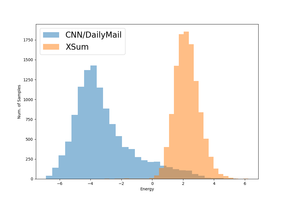
Figure 1: Energy histogram of the candidate summaries chosen by the EBR model on CNN/DailyMail and XSum.

6 Limitations and future work

Despite the improvements attained by our EBR model, its applicability is fundamentally dependent on the availability of reliable automatic evaluation metrics. Unfortunately, the correlation of these metrics with human judgment is still imperfect, especially for highly abstractive summaries. In addition, transformer-based metrics are currently only available for English. Finally, their backbone models are trained on news data, which hampers the reliability of these metrics in other domains. It is, therefore, crucial to continue the pursuit for more reliable metrics and to extend them to more languages and domains.

7 Conclusion

We proposed an energy-based re-ranking model that can be trained to rank candidate summaries according to a pre-specified metric, leveraging the recent advancements in automatic summarization metrics to enhance the quality of the generated summaries. The experiments show that the proposed re-ranking model succeeds at distilling the target metrics, consistently improving the scores of the generated summaries. However, these improvements not always agree with the human evaluation, especially in the more abstractive setting (XSum), due to flaws of the adopted target metrics (CTC scores). Nonetheless, the proposed approach is flexible in the sense that we can train it with any target metric and apply it in conjunction with virtually any abstractive summarization system.

Appendix A Further implementation details

A.1 Hyperparameters

To generate the training data for the re-ranking model, we sample $8$ candidate summaries for each source document using diverse beam search with a diversity weight of $0.8$. The candidates are then ranked according to the desired metric $\phi$ and the BERT model is fine-tuned on this data for up to $4$ epochs, with a batch size of $24$, and using the Adam optimizer Kingma and Ba (2014) with a learning rate of $5\times 10^{-5}$. We use $\tau=1$ (equation (2)) in all experiments. We keep the model that achieves the highest normalized discounted cumulative gain in a validation set. To generate the candidates at inference time, we set the diversity weight to zero since results in a separate validation set showed that this option yields the best results in most cases (see Appendix A.2). The models are implemented using the HuggingFace library on top of PyTorch. We also use HuggingFace publicly available checkpoints for the BART summarizers (facebook/bart-large-cnn and facebook/bart-large-xsum) and for BERT (bert-base-uncased).

A.2 Choice of the diversity weight

	Diversity weight	RL	QE	Cons	Rel
EBR-ListMLE [RL]	$0$	$43.50$	$\boldsymbol{43.57}$	$\boldsymbol{95.32}$	$\boldsymbol{63.28}$
Oracle [RL]		$46.95$	$43.37$	$95.26$	$64.54$
[0.5pt/5pt] EBR-ListMLE [RL]	$0.2$	$\boldsymbol{44.96}$	$42.83$	$90.61$	$59.54$
Oracle [RL]		$49.89$	$42.48$	$90.72$	$61.39$
[0.5pt/5pt] EBR-ListMLE [RL]	$0.5$	$44.98$	$42.83$	$90.47$	$59.53$
Oracle [RL]		$50.58$	$42.44$	$90.71$	$61.61$
[0.5pt/5pt] EBR-ListMLE [RL]	$0.8$	$44.92$	$42.81$	$90.32$	$59.42$
Oracle [RL]		$50.72$	$42.38$	$90.59$	$61.65$
EBR-ListMLE [QE]	$0$	$42.59$	$\boldsymbol{44.17}$	$\boldsymbol{95.93}$	$\boldsymbol{63.59}$
Oracle [QE]		$42.55$	$45.72$	$95.72$	$63.19$
[0.5pt/5pt] EBR-ListMLE [QE]	$0.2$	$44.01$	$43.92$	$92.57$	$60.82$
Oracle [QE]		$43.80$	$45.60$	$91.84$	$59.98$
[0.5pt/5pt] EBR-ListMLE [QE]	$0.5$	$\boldsymbol{44.08}$	$44.08$	$92.69$	$60.97$
Oracle [QE]		$43.92$	$45.84$	$91.87$	$60.15$
[0.5pt/5pt] EBR-ListMLE [QE]	$0.8$	$43.95$	$44.09$	$92.70$	$60.87$
Oracle [QE]		$43.74$	$45.88$	$91.81$	$60.00$
EBR-ListMLE [Rel]	$0$	$42.67$	$\boldsymbol{43.70}$	$\boldsymbol{96.11}$	$\boldsymbol{64.53}$
Oracle [Rel]		$44.32$	$43.52$	$96.24$	$66.40$
[0.5pt/5pt] EBR-ListMLE [Rel]	$0.2$	$43.83$	$43.24$	$93.77$	$62.26$
Oracle [Rel]		$46.04$	$42.87$	$93.56$	$64.52$
[0.5pt/5pt] EBR-ListMLE [Rel]	$0.5$	$\boldsymbol{43.87}$	$43.32$	$94.03$	$62.51$
Oracle [Rel]		$46.40$	$42.92$	$93.72$	$65.10$
[0.5pt/5pt] EBR-ListMLE [Rel]	$0.8$	$43.79$	$43.29$	$94.06$	$62.47$
Oracle [Rel]		$46.40$	$42.82$	$93.69$	$65.18$
EBR-ListMLE [Cons+Rel]	$0$	$42.49$	$\boldsymbol{43.69}$	$\boldsymbol{96.35}$	$\boldsymbol{64.45}$
Oracle [Cons+Rel]		$44.09$	$43.57$	$96.56$	$66.27$
[0.5pt/5pt] EBR-ListMLE [Cons+Rel]	$0.2$	$\boldsymbol{43.62}$	$43.24$	$94.21$	$62.25$
Oracle [Cons+Rel]		$45.30$	$43.00$	$94.42$	$64.20$
[0.5pt/5pt] EBR-ListMLE [Cons+Rel]	$0.5$	$43.50$	$43.24$	$94.52$	$62.44$
Oracle [Cons+Rel]		$45.56$	$43.09$	$94.67$	$64.74$
[0.5pt/5pt] EBR-ListMLE [Cons+Rel]	$0.8$	$43.43$	$43.21$	$94.56$	$62.46$
Oracle [Cons+Rel]		$45.42$	$43.02$	$94.70$	$64.79$

Table 5: Results (in %) for different diversity weights in a held-out validation set of CNN/DailyMail. (RL: ROUGE-L, QE: QuestEval, Cons: $\textnormal{CTC}_{\textnormal{consistency}}$, Rel: $\textnormal{CTC}_{\textnormal{relevance}}$)

Although we have used diverse beam search to generate the candidate summaries for training, we decided to stick to vanilla beam search for testing. This choice was made based on the results presented in Table 5. For this experiment, we have used a held-out development set from the validation set of CNN/DailyMail and we registered the results achieved by our EBR model and by an oracle re-ranker with diversity weights ranging from $0$ to $0.8$. According to all the metrics except ROUGE-L, setting the diversity weight to a positive value has a negative effect on the quality of the generated hypotheses since even an oracle re-ranker would have better results when the diversity weight is zero. Thus, we decided to set it at this value for the subsequent experiments with the test set.

Appendix B Ablation study

We now study the effect of training our EBR model using the max-margin loss proposed by Bhattacharyya et al. (2021) for machine translation. In addition, we also compare our models with perfect re-rankers for the two reference-free metrics: QuestEval and $\textnormal{CTC}_{\textnormal{consistency}}$. The results are in Table 6, where we also reproduce the results from our models presented in Table 1 for easier analysis. The comparison between the max-margin loss (EBR-MM) and ListMLE (EBR-ListMLE) shows that the latter tends to perform slightly better, although in the majority of the cases the difference is not statistically significant. It should also be remarked that re-ranking with the $\textnormal{CTC}_{\textnormal{consistency}}$ metric directly (Perfect Re-Rank [Cons]) yields competitive results too: it is the best on this metric in both datasets and it is close to the best model on $\textnormal{CTC}_{\textnormal{relevance}}$ in XSum. Re-ranking with QuestEval (Perfect Re-Rank [QE]) generally produces inferior results and, as shown previously in Table 2, has the additional inconvenience of being much slower.

	CNN/DailyMail							XSum
	R1	R2	RL	QE	Cons	Rel	FCC	R1	R2	RL	QE	Cons	Rel	FCC
Perfect Re-Rank [QE]	$43.91$	$20.99$	$40.76$	$\boldsymbol{45.74^{*}}$	$95.46$	$62.06$	$58.26$	$42.81$	$19.33$	$34.53$	$\boldsymbol{32.28^{*}}$	$83.31$	$52.57$	$26.58$
[0.5pt/5pt] Perfect Re-Rank [Cons]	$43.43$	$20.59$	$40.29$	$43.68$	$\boldsymbol{96.69^{*}}$	$62.60$	$\underline{61.36}$	$43.02$	$19.58$	$34.76$	$28.70$	$\boldsymbol{87.64^{*}}$	$54.33$	$\boldsymbol{27.61^{*}}$
EBR-MM [RL]	$\underline{44.49}$	$\underline{21.35}$	$\underline{41.32}$	$43.72$	$95.23$	$62.22$	$56.89$	$\boldsymbol{43.86}$	$\boldsymbol{20.30}$	$\underline{35.72}$	$28.68$	$83.32$	$52.85$	$25.98$
[0.5pt/5pt] EBR-MM [QE]	$44.07$	$21.13$	$40.93$	$44.22$	$95.70$	$62.54$	$59.49$	$42.85$	$19.42$	$34.54$	$29.63$	$83.37$	$52.58$	$25.86$
[0.5pt/5pt] EBR-MM [Rel]	$43.92$	$20.87$	$40.72$	$43.79$	$95.78$	$63.20$	$59.84$	$43.44$	$19.83$	$35.03$	$28.79$	$84.82$	$54.54$	$25.67$
[0.5pt/5pt] EBR-MM [Cons+Rel]	$43.75$	$20.78$	$40.56$	$43.78$	$95.98$	$63.10$	$60.75$	$43.31$	$19.76$	$34.95$	$28.83$	$85.42$	$54.50$	$26.38$
EBR-ListMLE [RL]	$\boldsymbol{44.90}$	$\boldsymbol{21.58}$	$\boldsymbol{41.75^{*}}$	$43.60$	$95.01$	$62.16$	$54.95$	$\underline{43.63}$	$\underline{20.28}$	$\boldsymbol{35.78}$	$28.55$	$84.47$	$52.92$	$\underline{27.21}$
[0.5pt/5pt] EBR-ListMLE [QE]	$44.07$	$21.13$	$40.94$	$\underline{44.27}$	$95.71$	$62.48$	$59.23$	$42.94$	$19.42$	$34.62$	$\underline{29.89}$	$83.34$	$52.50$	$26.34$
[0.5pt/5pt] EBR-ListMLE [Rel]	$44.04$	$20.98$	$40.85$	$43.78$	$95.93$	$\boldsymbol{63.40}$	$60.28$	$43.39$	$19.75$	$35.03$	$28.60$	$85.49$	$\boldsymbol{54.80}$	$26.28$
[0.5pt/5pt] EBR-ListMLE [Cons+Rel]	$43.88$	$20.87$	$40.69$	$43.79$	$\underline{96.15}$	$\underline{63.32}$	$\boldsymbol{61.67^{*}}$	$43.28$	$19.72$	$34.92$	$28.66$	$\underline{86.03}$	$\underline{54.74}$	$27.12$

Table 6: Results of our models (EBR-ListMLE) and baselines on each of the automatic evaluation metrics. Bold font indicates best result, and the second best results are underlined. A ^∗ mark indicates that the difference to the second best result is statistically significant (approximate permutation test at 95%). The metric in brackets indicates the target metric $\phi$ used to train the re-ranker. (R1: ROUGE-1, R2: ROUGE-2, RL: ROUGE-L, QE: QuestEval, Cons: $\textnormal{CTC}_{\textnormal{consistency}}$, Rel: $\textnormal{CTC}_{\textnormal{relevance}}$, FCC: FactCC)

Appendix C Effect of varying the number of candidates

Figure 2: Performance of the models on the CNN/DailyMail dataset according to the indicated metrics for different numbers of candidate summaries. (RL: ROUGE-L, QE: QuestEval, Cons: $\textnormal{CTC}_{\textnormal{consistency}}$, Rel: $\textnormal{CTC}_{\textnormal{relevance}}$)

Figure 2 shows the effect of varying the number of candidate summaries on the performance of our EBR models and BART baseline. The candidates were obtained using beam search with the number of beams equal to the number of candidates. The figure also shows the performance of the perfect re-ranker (Oracle), which defines the upper bound on the performance of the EBR.

Increasing the number of candidates leads to improvements in the performance of the EBR model when evaluated with the same metric it was trained to maximize. However, for ROUGE-L, these improvements are only marginal. Moreover, the performance gap between the Oracle and EBR tends to increase as well, especially in the reference-dependent metrics (ROUGE-L and $\textnormal{CTC}_{\textnormal{relevance}}$). The BART baseline also benefits from having larger beam sizes according to all metrics except ROUGE-L. Nonetheless, BART performs consistently worse than our EBR models according to all the metrics. Interestingly, increasing the number of candidates degrades ROUGE-L scores for all the models, except for EBR trained using this metric as the target.

Appendix D Human evaluation: further details

D.1 Evaluation form interface

The human evaluation form was built using the Google Forms platform. Figure 3 presents a screenshot of the user interface. As we can observe, the interface was divided into seven sections. The first one provides instructions to the user and a brief definition of each of the three evaluation criteria: “(1) - Factual consistency: A factually consistent summary should only contain exact, undistorted information that is present in the source text. No external information should be added.”; “(2) - Relevance: A relevant summary should provide the most important information presented in the source text.”; “(3) - Fluency: A fluent summary should be clear, grammatically correct, and sound like human-written text.”. The three subsequent sections present the source text followed by the two anonymized summaries. Finally, the last three sections contain the multiple choice questions for each of the evaluation criteria. This seven-section pattern repeats itself for all pairwise comparisons in the evaluation form.

Figure 3: Evaluation form

D.2 Detected factual inconsistencies

In Table 7 we show a few documents together with the summaries obtained from the baseline BART obtained with the usual beam search and the summaries chosen by the EBR model. Table 8 shows the examples from XSum used in the human evaluation questionnaire where the two judges agreed that the CLIFF summary was better than the EBR summary, regarding factual consistency. In two of the three examples, the $\textnormal{CTC}_{\textnormal{consistency}}$ metric wrongly assigns a larger score to the EBR summary than to the CLIFF summary. Interestingly, though, the EBR model would prefer the CLIFF summary over the BART summary in two of the three cases.

	Text	Cons	$E$
Source (CNN/DM)	Kell Brook has finally landed the Battle of Britain he craved, but will take on Frankie Gavin rather than bitter rival Amir Khan. Just sixty four days after the first defence of his IBF belt against Jo Jo Dan, Brook will return to action on a packed pay-per-view show on May 30 at the O2 in London. The welterweight bout has been added to a card that includes world title challenges for Kevin Mitchell and Lee Selby while Anthony Joshua faces his toughest test to date against Kevin Johnson. Kell Brook poses outside London’s O2 Arena where he will fight Frankie Gavin on May 30. Brook posing on the train as he headed to London for the announcement of his fight. Brook (left) was back in action as he beat Jo Jo Dan for the IBF World Welterweight title in Sheffield last month. Brook poses with Gavin inside the O2 arena after announcing their world title fight. Brook had been desperate to face Khan at Wembley in June but his compatriot ruled out a fight until at least later in the year. (…)
[0.5pt/5pt] BART	Kell Brook will fight Frankie Gavin at the O2 in London on May 30. The welterweight bout has been added to a card that includes world title challenges for Kevin Mitchell and Lee Selby. Anthony Joshua faces his toughest test to date against Kevin Johnson. Click here for more boxing news.	$88.6\%$	$0.09$
[0.5pt/5pt] EBR	Kell Brook will fight Frankie Gavin on May 30 at the O2 in London. The welterweight bout has been added to a card that includes world title challenges for Kevin Mitchell and Lee Selby. Anthony Joshua faces his toughest test to date against Kevin Johnson. Brook had been desperate to face Amir Khan at Wembley in June.	$\boldsymbol{97.3\%}$	$\boldsymbol{-3.67}$
Source (CNN/DM)	Aston Villa match-winner Fabian Delph was left pinching himself after booking his side’s place in the FA Cup final at the expense of Liverpool. Villa skipper Delph set up Christian Benteke’s equaliser after Philippe Coutinho opened the scoring for the Reds and then rounded off a superb afternoon by sweeping home nine minutes into the second half to secure a 2-1 victory. Delph’s strike means that Tim Sherwood’s charges will return to Wembley to face holders Arsenal in next month’s showpiece and the former Leeds midfielder says it will be a dream come true. Fabian Delph fires past Liverpool keeper Simon Mignolet to book Aston Villa’s place in the FA Cup final . Delph celebrates with team-mate Ashley Westwood after his 54th minute strike . Delph (left), Gabriel Agbonlahor (centre) and Grealish savour the winning feeling in the Villa dressing room . ’I can’t wait for the final. To walk out as captain is going to be the highlight of my career. So happy days, I’m happy for the boys,’ he told BT Sport 1. (…)"
[0.5pt/5pt] BART	Aston Villa beat Liverpool 2-1 in the FA Cup semi-final at Wembley. Fabian Delph scored the winning goal in the 54th minute. Tim Sherwood’s side will now face Arsenal in next month’s showpiece. Delph says the final will be the highlight of his career.	$85.3\%$	$1.22$
[0.5pt/5pt] EBR	Aston Villa beat Liverpool 2-1 in the FA Cup semi-final at Wembley. Fabian Delph scored the winning goal in the 54th minute. Tim Sherwood’s side will now face Arsenal in next month’s final. Delph says to walk out as captain in the final will be the highlight of his career.	$\boldsymbol{85.5\%}$	$\boldsymbol{0.73}$
Source (XSum)	The UN has said media restrictions and violence meant the environment was not conducive to free, credible elections. Unrest started in April after President Pierre Nkurunziza said he would run for a third term - something protesters say is illegal. The president says he is entitled to a third term because he was appointed for his first term, not elected. The presidential election is scheduled for 15 July. East African leaders have called for a further two-week delay. Africa news highlights: 7 July The electoral commission spokesman told the BBC turnout for the parliamentary poll had been low in the districts of Bujumbura where there had been protests, but that in some provinces outside the capital it was as high as 98The ruling party - the CNDD FDD - was ahead in every province of the country, Burundi’s electoral commission announced. They won 77 out of 100 elected seats in parliament, AFP news agency says. (…)
[0.5pt/5pt] BART	Burundi has held parliamentary elections, two months after the UN suspended its observer mission to the country.	$80.6\%$	$3.68$
[0.5pt/5pt] EBR	The ruling party in Burundi has won parliamentary elections, the first since a wave of protests began in April.	$\boldsymbol{83.7\%}$	$\boldsymbol{2.57}$
Source (XSum)	Many Sephardic Jews were killed, forced to convert to Christianity or leave at the end of the 15th Century. Parliament paved the way for a change in citizenship laws two years ago, but the move needed Cabinet approval. From now on, descendants of Sephardic Jews who can prove a strong link to Portugal can apply for a passport. Proof can be brought, the government says, through a combination of surname, language spoken in the family or evidence of direct descent. Thousands of Sephardic Jews were forced off the Iberian peninsula, first from Spain and then from Portugal. Some of those who fled to other parts of Europe or to America continued to speak a form of Portuguese in their new communities. The Portuguese government acknowledges that Jews lived in the region long before the Portuguese kingdom was founded in the 12th Century. (…)
[0.5pt/5pt] BART	Portugal has approved a law that will allow descendants of Jews who fled the country to become citizens.	$86.8\%$	$1.48$
[0.5pt/5pt] EBR	The Portuguese government has approved a law that will allow descendants of Jews who fled to Portugal to become citizens.	$\boldsymbol{93.1\%}$	$\boldsymbol{1.15}$

Table 7: Examples where the judges agreed that one of the summaries was better than the other on the factual consistency dimension. Consistent and inconsistent segments are highlighted in green and red, respectively. Columns Cons and $E$ show the $\textnormal{CTC}_{\textnormal{consistency}}$ (in %) and the energy score (output of the EBR model) on each of the summaries, respectively. (Remember that for $E$ lower is better.)

	Text	Cons	$E$
Source	Lance Naik (Corporal) Hanamanthappa Koppad was tapped under 8m of snow at a height of nearly 6,000m along with nine other soldiers who all died. Their bodies have now been recovered. The critically ill soldier has been airlifted to a hospital in Delhi. "We hope the miracle continues. Pray with us," an army statement said. The army added that "he has been placed on a ventilator to protect his airway and lungs in view of his comatose state". (…)
[0.5pt/5pt] CLIFF	An Indian soldier who was injured in an avalanche on the Siachen glacier in Indian-administered Kashmir last week is in a "comatose state", the army says.	$81.5$	$\boldsymbol{1.66}$
[0.5pt/5pt] EBR	A soldier who was trapped in an avalanche on the Siachen glacier in Indian-administered Kashmir last week has been declared dead, the army says.	$\boldsymbol{85.7}$	$1.82$
Source	They were among four people who were on Irish Coastguard Rescue 116 helicopter when it crashed on Tuesday. The funeral for pilot Captain Dara Fitzpatrick was held on Saturday. The search, which has been impeded by adverse weather, will also focus on finding the wreckage of the helicopter. The priority for those involved in the multi-agency operation has been to recover the bodies of chief pilot Mark Duffy and winchmen Paul Ormsby and Ciarán Smith. (…)
[0.5pt/5pt] CLIFF	The search for the bodies of three crew members who died in a helicopter crash off the coast of the Republic of Ireland has resumed.	$\boldsymbol{89.4}$	$\boldsymbol{3.24}$
[0.5pt/5pt] EBR	The search for two coastguard crew missing since a helicopter crash off the County Mayo coast has resumed.	$79.9$	$3.51$
Source	In the Yemeni capital, Sanaa, where the threat of attack is considered greatest, the UK, France and Germany have also shut their embassies. The British embassy has emptied completely, with all remaining British staff leaving the country on Tuesday, while the US air force flew out American personnel. So just what is it about al-Qaeda’s branch in Yemen that triggers such warning bells in Washington? Al-Qaeda in the Arabian Peninsula (AQAP), al-Qaeda’s branch in Yemen, is not the biggest offshoot of the late Osama Bin Laden’s organisation, nor is it necessarily the most active - there are other, noisier jihadist cells sprawled across Syria and Iraq, engaged in almost daily conflict with fellow Muslims. But Washington considers AQAP to be by far the most dangerous to the West because it has both technical skills and global reach. (…) According to the US think-tank the New America Foundation, US drone strikes in Yemen have soared, from 18 in 2011 to 53 in 2012. A drone strike on Tuesday reportedly hit a car carrying four al-Qaeda operatives. (…)
[0.5pt/5pt] CLIFF	The US has stepped up its drone strikes on al-Qaeda in the Arabian Peninsula (AQAP), a branch of the group that it considers the most dangerous to the West.	$76.8$	$3.57$
[0.5pt/5pt] EBR	The US has ordered all its diplomats to leave Yemen, saying it is under "heightened" US security concerns.	$\boldsymbol{80.3}$	$\boldsymbol{2.25}$

Table 8: Examples from XSum where the two judges agreed that CLIFF was better than EBR on the factual consistency dimension. Consistent and inconsistent segments are highlighted in green and red, respectively. Columns Cons and $E$ show the $\textnormal{CTC}_{\textnormal{consistency}}$ (in %) and the energy score (output of the EBR model) on each of the summaries, respectively. (Remember that for $E$ lower is better.)

References

- Aralikatte et al. (2021) Rahul Aralikatte, Shashi Narayan, Joshua Maynez, Sascha Rothe, and Ryan McDonald. 2021. Focus attention: Promoting faithfulness and diversity in summarization. In Proceedings of the 59th Annual Meeting of the Association for Computational Linguistics and the 11th International Joint Conference on Natural Language Processing (Volume 1: Long Papers), pages 6078–6095, Online. Association for Computational Linguistics.
- Bhattacharyya et al. (2021) Sumanta Bhattacharyya, Amirmohammad Rooshenas, Subhajit Naskar, Simeng Sun, Mohit Iyyer, and Andrew McCallum. 2021. Energy-based reranking: Improving neural machine translation using energy-based models. In Proceedings of the 59th Annual Meeting of the Association for Computational Linguistics and the 11th International Joint Conference on Natural Language Processing (Volume 1: Long Papers), pages 4528–4537, Online. Association for Computational Linguistics.
- Cao et al. (2020) Meng Cao, Yue Dong, Jiapeng Wu, and Jackie Chi Kit Cheung. 2020. Factual error correction for abstractive summarization models. In Proceedings of the 2020 Conference on Empirical Methods in Natural Language Processing (EMNLP), pages 6251–6258, Online. Association for Computational Linguistics.
- Cao and Wang (2021) Shuyang Cao and Lu Wang. 2021. CLIFF: Contrastive learning for improving faithfulness and factuality in abstractive summarization. In Proceedings of the 2021 Conference on Empirical Methods in Natural Language Processing, pages 6633–6649, Online and Punta Cana, Dominican Republic. Association for Computational Linguistics.
- Deng et al. (2021) Mingkai Deng, Bowen Tan, Zhengzhong Liu, Eric Xing, and Zhiting Hu. 2021. Compression, transduction, and creation: A unified framework for evaluating natural language generation. In Proceedings of the 2021 Conference on Empirical Methods in Natural Language Processing, pages 7580–7605, Online and Punta Cana, Dominican Republic. Association for Computational Linguistics.
- Devlin et al. (2019) Jacob Devlin, Ming-Wei Chang, Kenton Lee, and Kristina Toutanova. 2019. BERT: Pre-training of deep bidirectional transformers for language understanding. In Proceedings of the 2019 Conference of the North American Chapter of the Association for Computational Linguistics: Human Language Technologies, Volume 1 (Long and Short Papers), pages 4171–4186, Minneapolis, Minnesota. Association for Computational Linguistics.
- Durmus et al. (2020) Esin Durmus, He He, and Mona Diab. 2020. FEQA: A question answering evaluation framework for faithfulness assessment in abstractive summarization. In Proceedings of the 58th Annual Meeting of the Association for Computational Linguistics, pages 5055–5070, Online. Association for Computational Linguistics.
- Eikema et al. (2021) Bryan Eikema, Germán Kruszewski, Hady Elsahar, and Marc Dymetman. 2021. Sampling from discrete energy-based models with quality/efficiency trade-offs. arXiv preprint arXiv:2112.05702.
- Falke et al. (2019) Tobias Falke, Leonardo F. R. Ribeiro, Prasetya Ajie Utama, Ido Dagan, and Iryna Gurevych. 2019. Ranking generated summaries by correctness: An interesting but challenging application for natural language inference. In Proceedings of the 57th Annual Meeting of the Association for Computational Linguistics, pages 2214–2220, Florence, Italy. Association for Computational Linguistics.
- Fernandes et al. (2022) Patrick Fernandes, António Farinhas, Ricardo Rei, Perez Ogayo José G. C. de Souza, Graham Neubig, and André F. T. Martins. 2022. Quality-aware decoding for neural machine translation. In Proceedings of the meeting of North-American Association for Computational Linguistics.
- Goyal and Durrett (2021) Tanya Goyal and Greg Durrett. 2021. Annotating and modeling fine-grained factuality in summarization. In Proceedings of the 2021 Conference of the North American Chapter of the Association for Computational Linguistics: Human Language Technologies, pages 1449–1462, Online. Association for Computational Linguistics.
- Hermann et al. (2015) Karl Moritz Hermann, Tomas Kocisky, Edward Grefenstette, Lasse Espeholt, Will Kay, Mustafa Suleyman, and Phil Blunsom. 2015. Teaching machines to read and comprehend. Advances in neural information processing systems, 28.
- Kané et al. (2019) Hassan Kané, Yusuf Kocyigit, Pelkins Ajanoh, Ali Abdalla, and Mohamed Coulibali. 2019. Towards neural similarity evaluator. In Workshop on Document Intelligence at NeurIPS 2019.
- Kingma and Ba (2014) Diederik P Kingma and Jimmy Ba. 2014. Adam: A method for stochastic optimization. arXiv preprint arXiv:1412.6980.
- Kryscinski et al. (2019) Wojciech Kryscinski, Nitish Shirish Keskar, Bryan McCann, Caiming Xiong, and Richard Socher. 2019. Neural text summarization: A critical evaluation. In Proceedings of the 2019 Conference on Empirical Methods in Natural Language Processing and the 9th International Joint Conference on Natural Language Processing (EMNLP-IJCNLP), pages 540–551, Hong Kong, China. Association for Computational Linguistics.
- Kryscinski et al. (2020) Wojciech Kryscinski, Bryan McCann, Caiming Xiong, and Richard Socher. 2020. Evaluating the factual consistency of abstractive text summarization. In Proceedings of the 2020 Conference on Empirical Methods in Natural Language Processing (EMNLP), pages 9332–9346, Online. Association for Computational Linguistics.
- LeCun et al. (2006) Yann LeCun, Sumit Chopra, Raia Hadsell, M Ranzato, and F Huang. 2006. A tutorial on energy-based learning. Predicting structured data, 1(0).
- Lewis et al. (2020) Mike Lewis, Yinhan Liu, Naman Goyal, Marjan Ghazvininejad, Abdelrahman Mohamed, Omer Levy, Veselin Stoyanov, and Luke Zettlemoyer. 2020. BART: Denoising sequence-to-sequence pre-training for natural language generation, translation, and comprehension. In Proceedings of the 58th Annual Meeting of the Association for Computational Linguistics, pages 7871–7880, Online. Association for Computational Linguistics.
- Li et al. (2019) Siyao Li, Deren Lei, Pengda Qin, and William Yang Wang. 2019. Deep reinforcement learning with distributional semantic rewards for abstractive summarization. In Proceedings of the 2019 Conference on Empirical Methods in Natural Language Processing and the 9th International Joint Conference on Natural Language Processing (EMNLP-IJCNLP), pages 6038–6044, Hong Kong, China. Association for Computational Linguistics.
- Lin (2004) Chin-Yew Lin. 2004. ROUGE: A package for automatic evaluation of summaries. In Text Summarization Branches Out, pages 74–81, Barcelona, Spain. Association for Computational Linguistics.
- Liu et al. (2021) Wei Liu, Huanqin Wu, Wenjing Mu, Zhen Li, Tao Chen, and Dan Nie. 2021. Co2sum: Contrastive learning for factual-consistent abstractive summarization. arXiv preprint arXiv:2112.01147.
- Liu and Liu (2021) Yixin Liu and Pengfei Liu. 2021. SimCLS: A simple framework for contrastive learning of abstractive summarization. In Proceedings of the 59th Annual Meeting of the Association for Computational Linguistics and the 11th International Joint Conference on Natural Language Processing (Volume 2: Short Papers), pages 1065–1072, Online. Association for Computational Linguistics.
- Liu et al. (2022) Yixin Liu, Pengfei Liu, Dragomir Radev, and Graham Neubig. 2022. BRIO: Bringing order to abstractive summarization. In Proceedings of the 60th Annual Meeting of the Association for Computational Linguistics (Volume 1: Long Papers), pages 2890–2903, Dublin, Ireland. Association for Computational Linguistics.
- Lloret et al. (2018) Elena Lloret, Laura Plaza, and Ahmet Aker. 2018. The challenging task of summary evaluation: an overview. Language Resources and Evaluation, 52(1):101–148.
- Maynez et al. (2020) Joshua Maynez, Shashi Narayan, Bernd Bohnet, and Ryan McDonald. 2020. On faithfulness and factuality in abstractive summarization. In Proceedings of the 58th Annual Meeting of the Association for Computational Linguistics, pages 1906–1919, Online. Association for Computational Linguistics.
- Mizumoto and Matsumoto (2016) Tomoya Mizumoto and Yuji Matsumoto. 2016. Discriminative reranking for grammatical error correction with statistical machine translation. In Proceedings of the 2016 Conference of the North American Chapter of the Association for Computational Linguistics: Human Language Technologies, pages 1133–1138, San Diego, California. Association for Computational Linguistics.
- Narayan et al. (2018) Shashi Narayan, Shay B. Cohen, and Mirella Lapata. 2018. Don’t give me the details, just the summary! topic-aware convolutional neural networks for extreme summarization. In Proceedings of the 2018 Conference on Empirical Methods in Natural Language Processing, pages 1797–1807, Brussels, Belgium. Association for Computational Linguistics.
- Ng et al. (2019) Nathan Ng, Kyra Yee, Alexei Baevski, Myle Ott, Michael Auli, and Sergey Edunov. 2019. Facebook FAIR’s WMT19 news translation task submission. In Proceedings of the Fourth Conference on Machine Translation (Volume 2: Shared Task Papers, Day 1), pages 314–319, Florence, Italy. Association for Computational Linguistics.
- Papineni et al. (2002) Kishore Papineni, Salim Roukos, Todd Ward, and Wei-Jing Zhu. 2002. Bleu: a method for automatic evaluation of machine translation. In Proceedings of the 40th Annual Meeting of the Association for Computational Linguistics, pages 311–318, Philadelphia, Pennsylvania, USA. Association for Computational Linguistics.
- Paulus et al. (2018) Romain Paulus, Caiming Xiong, and Richard Socher. 2018. A deep reinforced model for abstractive summarization. In International Conference on Learning Representations.
- Raffel et al. (2020) Colin Raffel, Noam Shazeer, Adam Roberts, Katherine Lee, Sharan Narang, Michael Matena, Yanqi Zhou, Wei Li, and Peter J Liu. 2020. Exploring the limits of transfer learning with a unified text-to-text transformer. Journal of Machine Learning Research, 21:1–67.
- Ravaut et al. (2022) Mathieu Ravaut, Shafiq Joty, and Nancy Chen. 2022. SummaReranker: A multi-task mixture-of-experts re-ranking framework for abstractive summarization. In Proceedings of the 60th Annual Meeting of the Association for Computational Linguistics (Volume 1: Long Papers), pages 4504–4524, Dublin, Ireland. Association for Computational Linguistics.
- Salazar et al. (2020) Julian Salazar, Davis Liang, Toan Q. Nguyen, and Katrin Kirchhoff. 2020. Masked language model scoring. In Proceedings of the 58th Annual Meeting of the Association for Computational Linguistics, pages 2699–2712, Online. Association for Computational Linguistics.
- Scialom et al. (2021) Thomas Scialom, Paul-Alexis Dray, Sylvain Lamprier, Benjamin Piwowarski, Jacopo Staiano, Alex Wang, and Patrick Gallinari. 2021. QuestEval: Summarization asks for fact-based evaluation. In Proceedings of the 2021 Conference on Empirical Methods in Natural Language Processing, pages 6594–6604, Online and Punta Cana, Dominican Republic. Association for Computational Linguistics.
- Shen et al. (2004) Libin Shen, Anoop Sarkar, and Franz Josef Och. 2004. Discriminative reranking for machine translation. In Proceedings of the Human Language Technology Conference of the North American Chapter of the Association for Computational Linguistics: HLT-NAACL 2004, pages 177–184, Boston, Massachusetts, USA. Association for Computational Linguistics.
- Song and Kingma (2021) Yang Song and Diederik P Kingma. 2021. How to train your energy-based models. arXiv preprint arXiv:2101.03288.
- Tang et al. (2022) Xiangru Tang, Arjun Nair, Borui Wang, Bingyao Wang, Jai Desai, Aaron Wade, Haoran Li, Asli Celikyilmaz, Yashar Mehdad, and Dragomir Radev. 2022. CONFIT: Toward faithful dialogue summarization with linguistically-informed contrastive fine-tuning. In Proceedings of the 2022 Conference of the North American Chapter of the Association for Computational Linguistics: Human Language Technologies, pages 5657–5668, Seattle, United States. Association for Computational Linguistics.
- Vaswani et al. (2017) Ashish Vaswani, Noam Shazeer, Niki Parmar, Jakob Uszkoreit, Llion Jones, Aidan N Gomez, Łukasz Kaiser, and Illia Polosukhin. 2017. Attention is all you need. Advances in neural information processing systems, 30.
- Vijayakumar et al. (2016) Ashwin K Vijayakumar, Michael Cogswell, Ramprasath R Selvaraju, Qing Sun, Stefan Lee, David Crandall, and Dhruv Batra. 2016. Diverse beam search: Decoding diverse solutions from neural sequence models. arXiv preprint arXiv:1610.02424.
- Wang et al. (2020) Alex Wang, Kyunghyun Cho, and Mike Lewis. 2020. Asking and answering questions to evaluate the factual consistency of summaries. In Proceedings of the 58th Annual Meeting of the Association for Computational Linguistics, pages 5008–5020, Online. Association for Computational Linguistics.
- Xia et al. (2008) Fen Xia, Tie-Yan Liu, Jue Wang, Wensheng Zhang, and Hang Li. 2008. Listwise approach to learning to rank: theory and algorithm. In Proceedings of the 25th international conference on Machine learning, pages 1192–1199.
- Zhang et al. (2020) Jingqing Zhang, Yao Zhao, Mohammad Saleh, and Peter Liu. 2020. Pegasus: Pre-training with extracted gap-sentences for abstractive summarization. In International Conference on Machine Learning, pages 11328–11339. PMLR.
- Zhao et al. (2020) Zheng Zhao, Shay B. Cohen, and Bonnie Webber. 2020. Reducing quantity hallucinations in abstractive summarization. In Findings of the Association for Computational Linguistics: EMNLP 2020, pages 2237–2249, Online. Association for Computational Linguistics.
- Zhu et al. (2021) Chenguang Zhu, William Hinthorn, Ruochen Xu, Qingkai Zeng, Michael Zeng, Xuedong Huang, and Meng Jiang. 2021. Enhancing factual consistency of abstractive summarization. In Proceedings of the 2021 Conference of the North American Chapter of the Association for Computational Linguistics: Human Language Technologies, pages 718–733, Online. Association for Computational Linguistics.
- Zhuang et al. (2021) Liu Zhuang, Lin Wayne, Shi Ya, and Zhao Jun. 2021. A robustly optimized BERT pre-training approach with post-training. In Proceedings of the 20th Chinese National Conference on Computational Linguistics, pages 1218–1227, Huhhot, China. Chinese Information Processing Society of China.