Nonlinear Schrödinger equations with amplitude-dependent Wadati potentials

Abstract

Complex Wadati-type potentials of the form $V(x)=-w^{2}(x)+iw_{x}(x)$, where $w(x)$ is a real-valued function, are known to possess a number of intriguing features, unusual for generic non-Hermitian potentials. In the present work, we introduce a class of nonlinear Schrödinger-type problems which generalize the Wadati potentials by assuming that the base function $w(x)$ depends not only on the transverse spatial coordinate but also on the amplitude of the field. Several examples of prospective physical relevance are discussed, including models with the nonlinear dispersion or with the derivative nonlinearity. The numerical study indicates that the generalized model inherits the remarkable features of standard Wadati potentials, such as the existence of continuous soliton families, the possibility of symmetry-breaking bifurcations when the model obeys the parity-time symmetry, the existence of constant-amplitude waves, and the eigenvalue quartets in the linear-instability spectra. Our results deepen the current understanding of the interplay between nonlinearity and non-Hermiticity and expand the class of systems which enjoy the exceptional combination of properties unusual for generic dissipative nonlinear models.

I Introduction

The combination of nonlinearity and non-Hermiticity can have a dramatic impact on the properties of a waveguiding system. In particular, the presence of a non-Hermitian complex potential (which in physical terms takes into account the energy exchange with the environment) can heavily alter the structure of stationary localized nonlinear modes or solitons propagating in the system. While in conservative waveguides the solitons exist as continuous families parameterized by an ‘internal’ parameter, such as the soliton frequency or amplitude, the dissipative solitons most usually exist as isolated points AA ; Rosanov which, from the dynamical point of view, behave as attractors (provided that the soliton is stable). A prototypical model that illustrates this dissimilarity between conservative and dissipative systems is the generalized nonlinear Schrödinger equation (GNLSE)

$$i\Psi_{t}=-\Psi_{xx}+V(x)\Psi+W(x)F(|\Psi|^{2})\Psi,$$ (1)

where complex-valued functions $V(x)$ and $W(x)$ can be referred to as a linear and nonlinear potential, respectively, and real-valued function $F(\cdot)$, such that $F(0)=0$, specifies the nonlinearity. Equation (1) is a canonical model describing evolution of nonlinear waves in various physical settings. In particular, in optical applications, $\Psi$ corresponds to the dimensionless amplitude of the electric field. Its dependence on coordinate $t$ describes evolution of the pulse along the propagation direction, and $x$ is the transverse coordinate. Effective complex optical potentials correspond to the presence of spatial regions with gain and loss KYZ ; Ganainy , which, in particular, can be implemented using coherent multilevel atoms driven by external laser fields HH17 ; HHWadati .

When the imaginary parts of both potentials vanish, the model becomes conservative, and its stationary nonlinear modes $\Psi(x,t)=e^{-i\mu t}\psi(x)$ can be parameterized by the continuous change of the real frequency $\mu$. However, if at least one of the potentials is complex, then the continuous families of solitons typically disappear. At the same time, there exist at least two types of non-Hermitian potentials that do support continuous families of nonlinear modes (see a more detailed discussion in ZSA ). Systems of the first type obey the parity-time (${\cal PT}$) symmetry Bender ; KYZ : in this case real and imaginary parts of functions $V(x)$ and $W(x)$ are even and odd functions of $x$, respectively Musslimani ; AKKZ . The second type corresponds to the so-called Wadati-type potentials Wadati for which

$$V(x)=-w^{2}(x)+iw_{x}(x),\quad W(x)\equiv 1,$$ (2)

where $w(x)$ is a real-valued differentiable function which is not required to have any particular symmetry (at the same time, if $w(x)$ is even, then the resulting Wadati potential $V(x)$ becomes ${\cal PT}$ symmetric, i.e., the two types of potentials are partially overlapping). In what follows, it will be convenient to say that the GNLSE (1) with potentials (2) corresponds to linear Wadati potentials. Apart from the existence of continuous families of nonlinear modes Tsoy , linear Wadati potentials are known to support several other remarkable features. When the nonlinearity is absent, i.e., $F\equiv 0$, linear Wadati potentials can have all-real spectrum of eigenvalues NixonYang16PRA and undergo distinctive phase transition from all-real to complex spectrum through an exceptional point or a self-dual spectral singularity Yang17 ; ZK20 . Returning to the nonlinear setup, Wadati-type potentials support the existence of constant-amplitude nonlinear waves Makris , feature unusual dynamical behavior near the phase-transition threshold integral , and eigenvalue quartets in the linear-stability spectrum quartets . Additionally, when a Wadati potential is ${\cal PT}$ symmetric, it allows for bifurcations of families of non-${\cal PT}$-symmetric modes SB , which is impossible for ${\cal PT}$-symmetric potentials of general form. While the theory of Wadati potentials is far from being complete, on the qualitative level some of their peculiar properties can be explained by the existence of a ‘conserved’ (i.e., $x$-independent) quantity which constrains the shape of stationary modes KonZez14 .

Unusual and not yet fully understood properties of Wadati potentials encourage to look for their possible generalizations. In the meantime, most of the presently available studies of Wadati potentials are basically limited by GNLSE with spatially-uniform power-law and saturating nonlinearities NixonYang16 ; saturable . In the present paper, we introduce a more profound generalization of Wadati potentials by considering the situation where the base function $w(x)$ depends not only on the spatial coordinate $x$ but also on the amplitude of the field $\Psi$. We argue that the extended system preserves some of the properties of linear Wadati potentials. Particular realizations of the introduced generalization lead to nonlinear systems of potential physical relevance. Those include a GNLSE equation with the additional higher-order nonlinearity that emerges due to the stimulated response in optical fibers and a GNLSE with the derivative nonlinearity. Combining our analytical understandings with simple demonstrative computations, we construct continuous families of nonlinear modes and discuss their linearization spectra. Additionally, we show that when the generalized system is ${\cal PT}$ symmetric, it undergoes a symmetry-breaking bifurcation which results in continuous families of non-${\cal PT}$-symmetric solitons.

The rest of the paper is organized as follows. Section II outlines the derivation of the generalized model and presents several particular realizations of the extended system. Section III contains a case study of a model with the derivative nonlinearity. Section IV concludes the paper.

II Construction of generalized potentials

For stationary modes $\Psi(x,t)=e^{-i\mu t}\psi(x)$, equation (1) with linear Wadati potential (2) becomes

$$\mu\psi=-\psi_{xx}+(-w^{2}+iw_{x})\psi+F(|\psi|^{2})\psi.$$ (3)

The latter stationary equation has been studied in the previous literature Tsoy ; KonZez14 ; SB ; NixonYang16 ; saturable ; quartets ; BarZezKon ; Yang20 . In particular, it is known that if Eq. (3) is considered as a dynamical system with $x$ playing the role of the evolution variable, then the respective ‘dynamics’ is constrained by a conserved (i.e., $x$-independent) quantity KonZez14 . Our construction of the generalized model relies on a ‘gauge transformation’ which converts the stationary equation (3) to another ordinary differential equation, where the $x$-independent ‘integral of motion’ has an especially simple form unpublished . Indeed, using the substitution $\psi(x)=\phi(x)e^{i\int w(x)dx}$, where $\phi(x)$ is a new stationary field, from (3) we obtain

$$\mu\phi=-\phi_{xx}-2iw(x)\phi_{x}+F(|\phi|^{2})\phi.$$ (4)

Multiplying the latter equation by $\phi^{*}_{x}$ and adding it with its complex conjugate, we obtain the integral of motion

$$\mu|\phi|^{2}=-|\phi_{x}|^{2}+\int_{0}^{|\phi|^{2}}F(\xi)d\xi+\textrm{const},$$ (5)

where ‘const’ is an arbitrary $x$-independent quantity. Clearly, for localized modes with $\lim_{x\to\pm\infty}\phi(x)=\lim_{x\to\pm\infty}\phi_{x}(x)=0$ this constant must be zero. Using the obtained integral of motion as a qualitative argument, continuous families of nonlinear localized modes have been constructed in linear Wadati potentials KonZez14 . In the meantime, since the integral (5) does not contain function $w(x)$ explicitly, Eq. (4) can be generalized naturally by assuming that the base function $w(x)$ depends not only on the spatial coordinate $x$ but also on the amplitude of the field. This idea suggests to replace Eq. (4) with the following more general one:

$$\mu\phi=-\phi_{xx}-2iA(x,|\phi|^{2})\phi_{x}+F(|\phi|^{2})\phi,$$ (6)

where $A(\cdot,\cdot)$ is a real-valued function of two variables. It is easy to check that the identity (5) remains valid for the newly introduced Eq. (6). We further make the ‘inverse’ gauge transformation $\phi(x)=\psi(x)e^{i\int z(x)dx}$, where $z(x):=B(x,|\psi|^{2})$ is another real-valued function, which converts (6) into the following equation:

$$\mu\psi=-\psi_{xx}+\left(2AB+B^{2}-i\frac{\partial B(x,|\psi|^{2})}{\partial x}-i\frac{\partial B(x,|\psi|^{2})}{\partial|\psi|^{2}}(|\psi|^{2})_{x}\right)\psi-2i(A+B)\psi_{x}+F(|\psi|^{2})\psi.$$ (7)

The obtained stationary equation corresponds to the following temporal evolution problem:

$$i\Psi_{t}=-\Psi_{xx}+\left(2AB+B^{2}-i\frac{\partial B(x,|\Psi|^{2})}{\partial x}-i\frac{\partial B(x,|\Psi|^{2})}{\partial|\Psi|^{2}}(|\Psi|^{2})_{x}\right)\Psi-2i(A+B)\Psi_{x}+F(|\Psi|^{2})\Psi.$$ (8)

Equation (8) is the central point of the present paper. It represents the generalization of the previously studied GNLSE with linear Wadati potentials, which can be recovered from Eq. (8) by setting $A=-B=w(x)$. To distinguish this model from the known case of linear Wadati potentials, we will say that Eq. (8) corresponds to nonlinear Wadati potentials. By construction, the stationary version of this model [i.e., Eq. (7)] has the $x$-independent conserved quantity and is therefore expected to support continuous families of nonlinear localized modes and share other properties of linear Wadati potentials.

For different choices of $A$ and $B$ the obtained equation (8) acquires specific shapes which can be of potential relevance for physical applications.

Example 1.

Choosing $A=-B=w(x)+\sigma|\Psi|^{2}$, where $\sigma$ is a real coefficient, from (8) we obtain the following equation:

$$i\Psi_{t}=-\Psi_{xx}+(-w^{2}+iw_{x})\Psi-2\sigma w(x)|\Psi|^{2}\Psi$$

$$-\sigma^{2}|\Psi|^{4}\Psi+i\sigma(|\Psi|^{2})_{x}\Psi+F(|\Psi|^{2})\Psi.$$ (9)

The case $\sigma=0$ recovers the previously considered GNLSE with linear Wadati potentials. Let us comment on the newly appeared terms that contain the coefficient $\sigma$. The term $2\sigma w(x)|\Psi|^{2}\Psi$ can be considered as cubic nonlinearity with a real-valued nonlinear potential whose spatial shape is given by the base function $w(x)$. The term $\sigma^{2}|\Psi|^{4}\Psi$ corresponds to the spatially uniform quintic focusing nonlinearity. Assuming that $\sigma$ is small, this term can be neglected in the leading order. In fact this term can be ‘eliminated’ by a simple redefinition of function $F$. The most unconventional term in Eq. (9) corresponds to $i\sigma(|\Psi|^{2})_{x}\Psi$. In fiber optics, the higher-order nonlinear terms of this form have been used to take into account nonlinear dispersion resulting from the stimulated Raman scattering (SRS) of ultrashort pulses, see e.g. SRS1 ; SRS2 ; SRS3 ; SRS4 .

Example 2.

Choosing $A=-B=\sigma w(x)|\Psi|^{2}$, we arrive at the following equation, where the nonlinear gain-and-loss term and nonlinear dispersion are spatially modulated by function $w(x)$ and its derivative $w_{x}(x)$:

$$i\Psi_{t}=-\Psi_{xx}+(-\sigma^{2}w^{2}|\Psi|^{4}+i\sigma w_{x}|\Psi|^{2})\Psi$$

$$+i\sigma w(x)(|\Psi|^{2})_{x}\Psi+F(|\Psi|^{2})\Psi.$$ (10)

Example 3.

The choice $A=w(x)-\sigma|\Psi|^{2}/2$ and $B=-w(x)+\sigma|\Psi|^{2}$ transforms equation (8) to the following model:

$$i\Psi_{t}=-\Psi_{xx}+(-w^{2}+iw_{x})\Psi+\sigma w(x)|\Psi|^{2}\Psi$$

$$+F(|\Psi|^{2})\Psi-i\sigma(|\Psi|^{2}\Psi)_{x}.$$ (11)

In the latter equation, the spatially inhomogeneous cubic nonlinearity $\sigma w(x)|\Psi|^{2}\Psi$ is present together with the derivative nonlinearity $i\sigma(|\Psi|^{2}\Psi)_{x}$. The derivative NLSE $i\Psi_{t}=-\Psi_{xx}-i\sigma(|\Psi|^{2}\Psi)_{x}$ is integrable by the inverse scattering method Kaup ; CCL and has been widely used to describe nonlinear waves in plasma Miolhus ; Mio and optical fibers Agrawal . Notice that the ‘additional’ terms in Eq. (11) (i.e., those with coefficient $\sigma$) are conservative, i.e., do not contribute to the power balance equation: indeed, introducing the power $P(t)=\int_{-\infty}^{\infty}|\Psi|^{2}dx$, from Eq. (11) we compute

$$\frac{dP(t)}{dt}=2\int_{-\infty}^{\infty}w_{x}|\Psi|^{2}dx.$$ (12)

Several recent studies have addressed the derivative NLSE with ${\cal PT}$-symmetric potentials Saleh14 ; DNLS1 ; DNLS2 ; DNLS3 . Being motivated, in part, by this newly emerged interest in non-Hermitian extensions of the derivative NLSE, in the next section, we perform a more detailed examination of the model (11).

III Wadati potentials with the derivative nonlinearity

III.1 Constant-amplitude waves

In spite of their spatially inhomogeneous structure, the linear Wadati potentials are known to support constant-amplitude solutions Makris . Similar solutions can be found in the introduced generalized models. They can be constructed easily by noticing that a pair $\phi(x)\equiv\rho_{0}$ and $\mu=F(\rho_{0}^{2})$, where $\rho_{0}$ is arbitrary real amplitude, solves Eq. (4). In particular, for Eq. (11) the constant-amplitude solution reads

$$\Psi(x,t)=\rho_{0}\exp\left\{i\int w(x)dx-i\sigma\rho_{0}^{2}x-iF(\rho_{0}^{2})t\right\}.$$ (13)

In linear Wadati potentials, constant-amplitude waves of the analogous form have been used to examine the development of modulational instability in non-Hermitian optical media Makris and to implement coherent perfect absorption of nonlinear waves ZK20 .

III.2 Computing the continuous families of nonlinear modes using the numerical shooting approach

Let us now use the demonstrative computation to argue that Eq. (11) supports continuous families of stationary localized modes $\Psi=e^{-i\mu t}\psi(x)$, where $\mu$ is a real parameter, and $\lim_{x\to\pm\infty}\psi(x)=0$. The corresponding procedure is essentially a generalization of the approach from KonZez14 . It is more convenient to describe it in terms of the equivalent Eq. (6). We reduce the dimensionality of the underlying phase space by employing the representation $\phi(x)=\rho(x)\exp\{i\int v(x)dx\}$, where $\rho(x)$ and $v(x)$ are real-valued functions. Separating Eq. (6) into real and imaginary parts, we arrive at the system

$$\mu\rho=-\rho_{xx}+v^{2}\rho+2A(x,\rho^{2})v\rho+F(\rho^{2})\rho,$$ (14)

$$-v_{x}\rho-2v\rho_{x}-2A(x,\rho^{2})\rho_{x}=0.$$ (15)

We fix some $\mu<0$ and assume that $A(x,\rho^{2}(x))$ decays fast as $x\to\pm\infty$. Then solutions $\phi_{\pm}(x)$ that decay, respectively, at $+\infty$ and $-\infty$ have simple asymptotic behavior $\phi_{\pm}(x)=e^{-\sqrt{|\mu|}|x|}(C_{\pm}+o(1)_{x\to\pm\infty})$, where $C_{\pm}$ are real $x$-independent constants. The asymptotic behavior of derivatives $\phi_{x,\pm}(x)$ can be obtained by differentiating the asymptotic equations for $\phi_{\pm}(x)$. Choosing some sufficiently large $x_{\infty}\gg 1$, for any $C_{+}$ and $C_{-}$ we can use the found asymptotic behavior to approximate $(\rho_{\pm}(\pm x_{\infty}),\rho_{x,\pm}(\pm x_{\infty}),v_{\pm}(\pm x_{\infty}))$ and then use those as initial values for numerical solution of system (14)–(15), computing in this way solutions $(\rho_{+}(x),\rho_{x,+}(x),v_{+}(x))$ on the interval $[0,x_{\infty})$ and $(\rho_{-}(x),\rho_{x,-}(x),v_{-}(x))$ on the interval $(-x_{\infty},0]$. Looking for a continuously differentiable localized mode $\phi(x)$ which decays at both infinities, we need to find a solution to the following system of three equations:

$$\rho_{+}(0)=\rho_{-}(0),\quad\rho_{+,x}(0)=\rho_{-,x}(0),\quad v_{+}(0)=v_{-}(0)$$ (16)

with respect to two unknowns (i.e., two ‘shooting parameters’) $C_{+}$ and $C_{-}$. At first glance, system (16) seems overdetermined and therefore is not expected to have a solution. However, the integral (5) imposes an additional relation between the functions: $\mu\rho_{\pm}^{2}(x)=-\rho_{\pm,x}^{2}(x)-v^{2}_{\pm}(x)\rho_{\pm}^{2}(x)+\int_{0}^{\rho_{\pm}^{2}(x)}F(\xi)d\xi$. These constraints imply that if any two equations (say the first two) of system (16) are satisfied, then the third equation is satisfied automatically (speaking more precisely, the third equation will be satisfied in the form $v_{+}^{2}(0)=v_{-}^{2}(0)$; however, the spurious solutions with $v_{+}(0)=-v_{-}(0)$ can be easily filtered out in the practical realization of the procedure). Therefore, system (16) is not overdetermined and can be expected to have one or several solutions each of which corresponds to a localized mode. Since the described procedure can be fulfilled for any $\mu<0$, the continuous in $\mu$ families of localized modes are indeed expected to exist.

Proceeding now to a numerical illustration, we look for stationary modes of equation (11) with the derivative nonlinearity and therefore consider $A(x,\rho^{2}(x))=w(x)-\sigma\rho^{2}(x)/2$ with an asymmetric base function $w(x)$ in the form

$$w(x)=\tanh 2(x-2.5)-\tanh(x-2.5).$$ (17)

For linear Wadati potentials, this base function has been considered in quartets . To keep the model as simple as possible but still nontrivial, in this example we remove the conventional nonlinearity by setting $F\equiv 0$. In Fig. 1(a) we illustrate the numerical shooting procedure by presenting the dependencies $\rho_{+}(0)$ vs. $\rho_{+,x}(0)$ and $\rho_{-}(0)$ vs. $\rho_{-,x}(0)$ obtained from the numerical solution of the system (14)–(15) under the gradual increase of shooting parameters $C_{+}$ and $C_{-}$ departing from zero, and for fixed value of $\mu$. Apart from the origin (which corresponds to the trivial zero solution with $C_{+}=C_{-}=0$), the shown curves feature two intersections, which correspond to the particular values of the shooting parameters $(C_{+},C_{-})$ for which the first two equations of system (16) are satisfied. It has been checked that the third equation of this system is also satisfied for both intersections and hence they indeed correspond to two localized modes. Spatial profiles $|\psi(x)|=|\phi(x)|$ of these modes are shown in Fig. 1(b). Gradually changing $\mu$ and tracing the found intersections, we construct two continuous families which are visualized in Fig. 1(c) in the form of continuous dependencies $P(\mu)$, where $P=\int_{-\infty}^{\infty}|\psi|^{2}dx$ is the squared $L^{2}$-norm of the solution (that corresponds to the optical beam power). In the limit $P\to 0$ the solutions become small-amplitude, and the corresponding values of $\mu$ approach the eigenvalues of the underlying linear eigenvalue problem which can be formally obtained from (3) by setting $F(|\psi|^{2})=0$.

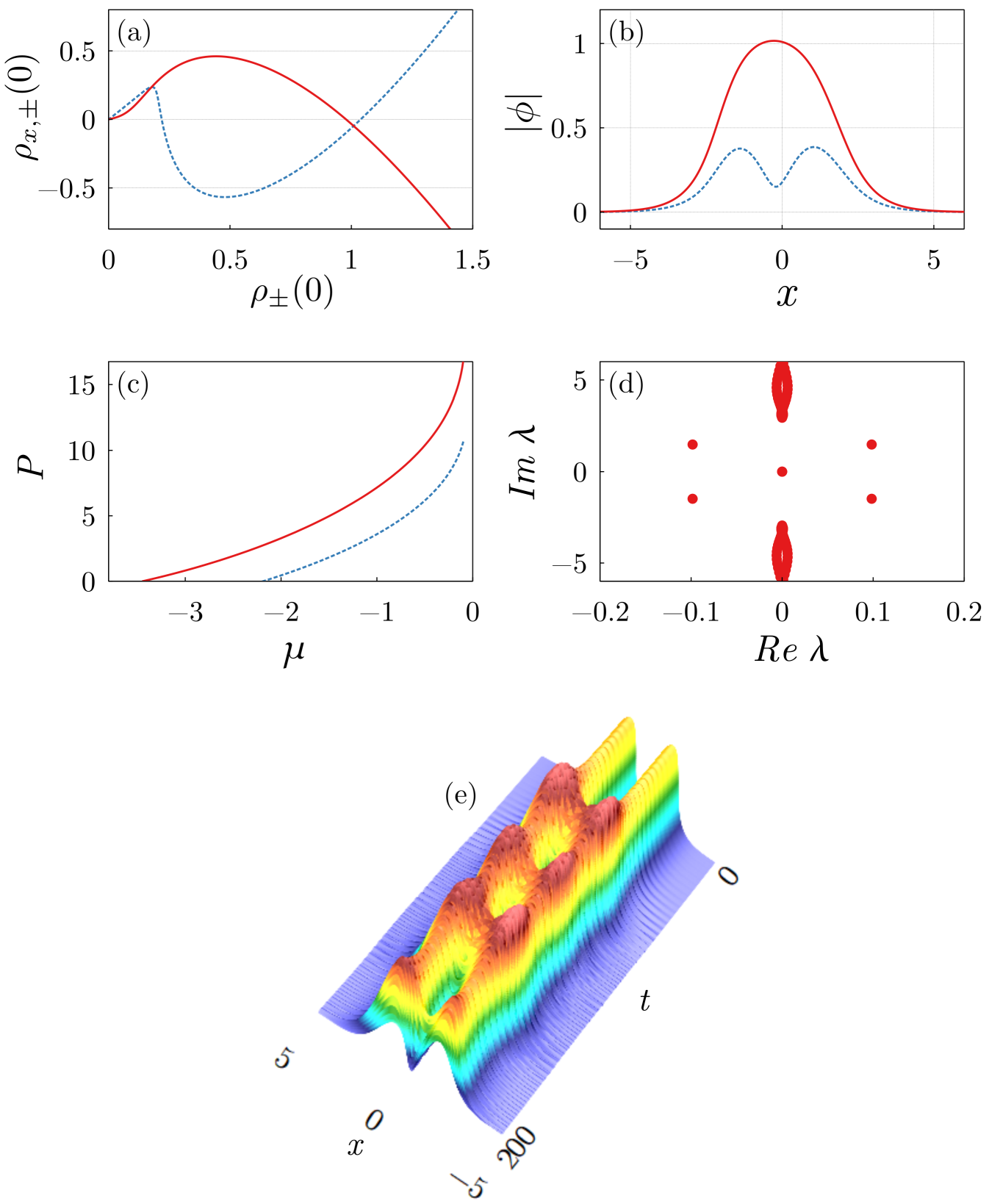
Figure 1: (a) Dependencies $\rho_{+}(0)$ vs. $\rho_{+,x}(0)$ (solid red curve) and $\rho_{-}(0)$ vs. $\rho_{-,x}(0)$ (dotted blue curve) obtained by the numerical shooting procedure for $\mu=-2$. (b) Amplitudes of nonlinear modes $|\psi(x)|=|\phi(x)|$ corresponding to the two intersections in (a). Solid red and dotted blue profiles correspond to the fundamental and first excited states, respectively. (c) Continuous curves corresponding to the families of fundamental (solid red curve) and first excited (dotted blue curve) nonlinear modes. In (a)-(c) we use $F(|\psi|^{2})=0$ and $\sigma=1$. (d) Linear stability eigenvalues $\lambda$ (shown with red circles) for the mode from the excited family at $\mu=-3$ for $F(|\psi|^{2})=-|\psi|^{2}$ and $\sigma=0.25$. (e) Temporal evolution $|\Psi(x,t)|$ of an initial condition taken as a slightly perturbed stationary mode whose linear-instability spectrum is shown in (d).

While the discussion in this subsection has been limited to the spatially localized modes whose amplitude $|\rho(x)|$ vanishes rapidly enough as $x\to\infty$ and $x\to-\infty$, the consideration can be extended toward inclusion of stationary modes with nonvanishing asymptotic behavior. In particular, similar arguments can be elaborated for kink-like solutions with $\lim_{x\to\pm\infty}\rho(x)=r_{\pm}$, where $r_{+}$ and $r_{-}$ are nonzero constants, provided that the corresponding asymptotic behavior can be exhaustively described using several shooting parameters.

III.3 Eigenvalue quartets in the linear-instability spectrum

For linear Wadati potentials, it has been found numerically that the complex eigenvalues of the linear-stability operator always appear in quartets $(\lambda,\lambda^{*},-\lambda,-\lambda^{*})$ quartets . This numerical observation (which, to the best of our knowledge, has not yet received any analytical confirmation) is rather intriguing, because the eigenvalue quartets are more typical to Hamiltonian systems or to setups constrained by some explicit symmetry (such as ${\cal PT}$-symmetric systems). In the meantime, the GNLSE with Wadati potentials does not apparently feature a Hamiltonian structure and has no readily evident symmetry. In order to examine if the eigenvalue quartets persist in our generalized model, we perform the standard linearization procedure using the perturbed stationary-mode substitution in the form $\Psi(x,t)=e^{-i\mu t}[\psi(x)+a(x)e^{\lambda t}+b^{*}(x)e^{\lambda^{*}t}]$, where $a(x)$ and $b(x)$ are small perturbations, and complex $\lambda$ is linear stability eigenvalue. Positive real part of $\lambda$ defines the increment of an eventual instability. Using this substitution in Eq. (11) and keeping only the linear in $a(x)$ and $b(x)$ terms, we obtain a linear-stability eigenproblem for eigenvalue $\lambda$ and eigenvector $(a,b)^{T}$ (since the linearization procedure is straightforward, we do not present the corresponding linear stability equations herein). For a numerical illustration we consider Eq. (11) with the the base function given by (17) and cubic nonlinearity $F(|\psi|^{2})=-|\psi|^{2}$. Then for $\sigma=0$ our model recovers that from quartets , where the existence of quartets has been observed numerically. Increasing $\sigma$ and evaluating numerically the linear-stability spectra, we observe that the eigenvalue quartets persist for $\sigma\neq 0$. For example, for $\mu=-3$ and $\sigma=0.25$ we obtain eigenvalues $\lambda_{1,2}\approx 0.0983725\pm i1.484634$ and $\lambda_{3,4}\approx-0.0983725\pm i1.484634$, i.e., the numerical results allow to conjecture the found eigenvalues indeed form a quartet, at least with the accuracy $~{}10^{-6}$. A rigorous proof of this fact remains an interesting issue for future studies.

To corroborate the presence of the instability, we have simulated nonlinear dynamics governed by Eq. (11) using a modification of the finite-difference Crank-Nicolson scheme adapted for the derivative nonlinearity LiLiShi ; GuoFang . Choosing the slightly perturbed unstable stationary mode as an initial condition, from its evolution shown in Fig. 1(e) we observe that the stationary mode preserves its shape for $t\lesssim 50$, but for larger times the shape of numerical solution oscillates aperiodically.

III.4 Symmetry-breaking bifurcation and non-${\cal PT}$-symmetric modes in the ${\cal PT}$-symmetric case

Next, we illustrate that in the case when the introduced generalized model becomes ${\cal PT}$ symmetric, it can support asymmetric (more precisely, not ${\cal PT}$ symmetric) nonlinear modes. As in the case of linear Wadati potentials, Eq. (11) becomes ${\cal PT}$ symmetric Bender , i.e., invariant under the transformation $x\to-x$, $t\to-t$ and $i\to-i$, when the base function $w(x)$ is even. Symmetric and asymmetric modes can be searched using the numerical shooting approach outlined above. For a numerical illustration, we use a bimodal base function in the form $w(x)=2e^{-(x-1.2)^{2}}+2e^{-(x+1.2)^{2}}$ which results in an effectively double-well potential. In Fig. 2(a) we plot the corresponding dependencies $\rho_{+}(0)$ vs. $\rho_{+,x}(0)$ and $\rho_{-}(0)$ vs. $\rho_{-,x}(0)$. Three intersections in Fig. 2(a) correspond to a pair of asymmetric modes (the two intersections with $\rho_{x}(0)\neq 0$) and to a ${\cal PT}$-symmetric mode (the intersection with $\rho_{x}(0)=0$). Spatial profiles of symmetric and asymmetric modes are plotted in Fig. 2(b). Changing the value of $\mu$, we construct continuous families of ${\cal PT}$-symmetric and asymmetric modes. Two asymmetric families bifurcate from the symmetric one after a supercritical pitchfork bifurcation: in other words, the symmetric family is stable for small $P$, but becomes unstable right after the bifurcation. A representative plot of linear stability eigenvalues for the symmetric family past the symmetry-breaking bifurcation is plotted in Fig. 2(d). In Fig. 3 we present several representative examples of numerically computed nonlinear dynamics in the ${\cal PT}$-symmetric system. In agreement with the predictions of the linear-stability analysis, we observe that above the symmetry-breaking bifurcation the symmetric family is unstable [Fig. 3(a)]: the initially perturbed symmetric stationary mode shortly evolves to a breather-like oscillating entity. The asymmetric families [Fig. 3(b)] and the symmetric family below the symmetry-breaking bifurcation are stable, and the corresponding numerical solutions preserve the stationary shape for indefinitely long time.

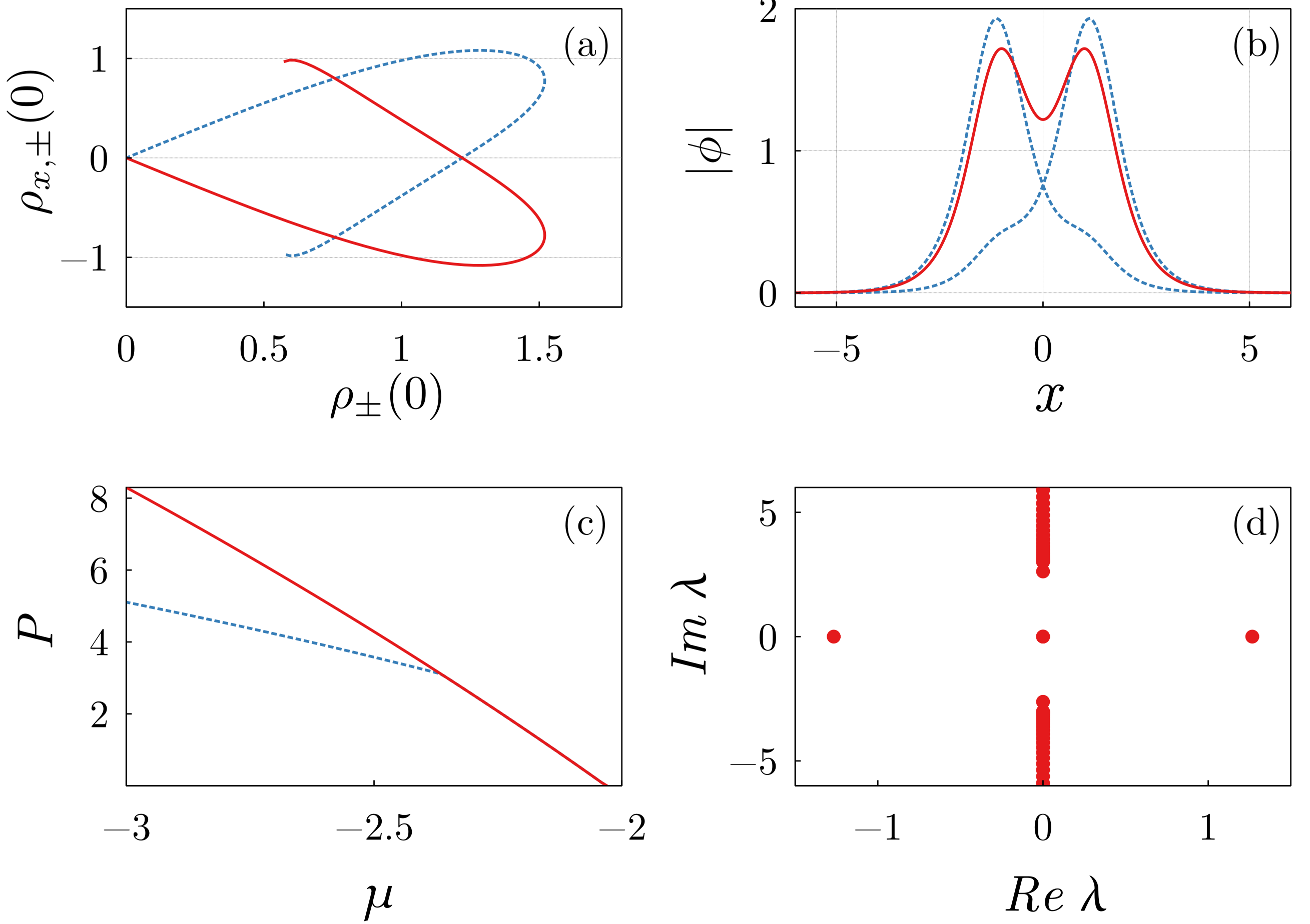
Figure 2: (a) Dependencies $\rho_{+}(0)$ vs. $\rho_{+,x}(0)$ (solid red curve) and $\rho_{-}(0)$ vs. $\rho_{-,x}(0)$ (dotted blue curve) obtained by the numerical shooting procedure for ${\cal PT}$-symmetric system at $\mu=-3$ constructed by increasing the shooting parameters from $C_{\pm}=0$ to $C_{\pm}=34$. (b) Amplitudes of nonlinear modes corresponding to the intersections in (a). Solid red curve corresponds to the ${\cal PT}$-symmetric soliton and two dotted blue profiles correspond to a pair of symmetry-broken solitons. (c) Continuous families of ${\cal PT}$-symmetric (solid red curve) and asymmetric (dotted blue curve) solitons. (d) Linear stability eigenvalues for the ${\cal PT}$-symmetric soliton at $\mu=-3$. In this figure $F(|\psi|^{2})=-|\psi|^{2}$ and $\sigma=0.4$.

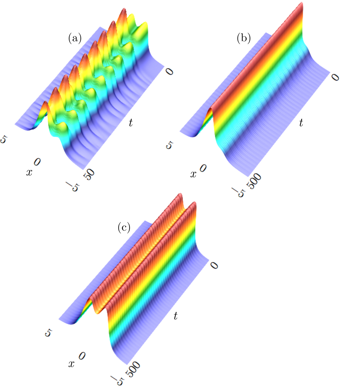
Figure 3: Temporal evolutions of initial conditions taken as slightly perturbed stationary modes from Fig. 2: unstable symmetric (a) and stable asymmetric (b) modes above the symmetry-breaking bifurcation (specifically, at $\mu=-3$) and stable symmetric mode below the symmetry-breaking bifurcation (specifically, at $\mu=-2.2$). The plots show $|\Psi(x,t)|$.

III.5 Absence of the dynamical conservation law

Results of the previous subsections do not imply that nonlinear Wadati potentials simply inherit any property of linear Wadati potentials without even a minor modification. As an example of a dissimilarity between the two types of potentials, we recall that linear Wadati potentials admit a dynamical (i.e., $t$-independent) conserved quantity given as integral

$$J=\int_{-\infty}^{\infty}[i\Psi\Psi_{x}^{*}-w(x)|\Psi|^{2}]dx.$$ (18)

Indeed, for linear Wadati potentials from Eqs. (1)–(2) we compute $dJ/dt=0$. In the meantime, for nonlinear Wadati potentials from Eq. (11) we evaluate

$$\frac{dJ}{dt}=\sigma\int_{-\infty}^{\infty}\left[2w(|\Psi|^{4})_{x}dx+i(|\Psi|^{2})_{x}(\Psi_{x}\Psi^{*}-\Psi_{x}^{*}\Psi)\right]dx$$

$$=\sigma\int_{-\infty}^{\infty}(|\Psi|^{4})_{x}[2w-(\arg\Psi)_{x}]dx.$$

Hence the dynamical conserved quantity (18) does not carry over to nonlinear Wadati potentials. Of course, this does not imply that the extended model (11) does not have any dynamical conservation law at all. However, so far we have not been able to find a generalization of the dynamical integral (18) for nonlinear Wadati potentials.

IV Conclusion

Nonlinear Schrödinger equation with complex Wadati-type potentials is known to feature a variety of unusual and intriguing properties. In the meantime, the generalizations of Wadati potentials are rather scarce, and most of the activity in this direction is presently limited by spatially homogeneous power-law and saturating nonlinearities. In this paper, we have proposed a significant extension of Wadati potentials. The main idea of our approach is to consider the base function of a Wadati potential as depending not only on the spatial coordinate but also on the amplitude of the field. The resulting extended model admits a conserved (i.e., independent of the transverse coordinate) quantity. Using this conserved quantity, we have employed a demonstrative computation approach to argue that the generalized model supports continuous families of bright solitons. The numerical study of the linear-instability spectra indicates that unstable solitons feature eigenvalue quartets, which is another remarkable peculiarity of Wadati potentials. We have demonstrated that the generalized parity-time-symmetric model supports a supercritical symmetry-breaking bifurcation that gives birth to continuous families of non-${\cal PT}$-symmetric solitons. Numerical simulations of nonlinear dynamics indicate that unstable stationary modes can dynamically transform to nearly periodic breather-like solutions. The introduced model also admits a straightforward generalization of constant-amplitude nonlinear waves known to exist in conventional Wadati potentials. In contrast to the previously known models with Wadati potentials, our generalization incorporates spatially modulated nonlinearity, where the shape of the modulation is determined by the base function of the Wadati potential. Additional nonlinear terms can include spatially-uniform nonlinear dispersion or derivative nonlinearity. Our findings essentially broaden the class of systems which enjoy the unique combination of peculiar features of nonlinear and non-Hermitian systems typical to Wadati-type and ${\cal PT}$-symmetric potentials.

References

- (1) N. Akhmediev and A. Ankiewicz, Three sources and three component parts of the concept of dissipative solitons. In: Akhmediev N, Ankiewicz A, eds. Dissipative Solitons: From Optics to Biology and Medicine. Springer-Verlag; 2008: 1–29.
- (2) N. N. Rozanov, Dissipative optical solitons, J. Opt. Technol. 76, 187 (2009).
- (3) V. V. Konotop, J. Yang, and D. A. Zezyulin, Nonlinear waves in -symmetric systems, Rev. Mod. Phys. 88, 035002 (2016).
- (4) R. El-Ganainy, K. G. Makris, M. Khajavikhan, Z. H. Musslimani, S. Rotter, and D. N. Christodoulides, Non-Hermitian physics and PT symmetry, Nature Phys. 14, 11 (2018).
- (5) C. Hang and G. Huang, Parity-time symmetry with coherent atomic gases, Advances in Physics: X 2, 737 (2017).
- (6) C. Hang, G. Gabadadze, and G. Huang, Realization of non--symmetric optical potentials with all-real spectra in a coherent atomic system, Phys. Rev. A 95, 023833 (2017).
- (7) D. A. Zezyulin, A. O. Slobodyanyuk, G. L. Alfimov, On nonexistence of continuous families of stationary nonlinear modes for a class of complex potentials, Stud. Appl. Math. 148, 99–124 (2022).
- (8) C. M. Bender and S. Boettcher, Real Spectra in Non-Hermitian Hamiltonians Having Symmetry, Phys. Rev. Lett. 80, 5243 (1998).
- (9) Z. H. Musslimani, K. G. Makris, R. El Ganainy D. N. Christodoulides, Optical solitons in PT-periodic potentials, Phys. Rev. Lett. 100, 030402 (2008).
- (10) F. Kh. Abdullaev, Y. V. Kartashov, V. V. Konotop, and D. A. Zezyulin, Solitons in -symmetric nonlinear lattices, Phys. Rev. A 83, 041805(R) (2011).
- (11) M. Wadati, Construction of parity-time symmetric potential through the soliton theory, J. Phys. Soc. Jpn. 77, 074005 (2008).
- (12) E. N. Tsoy, I. M. Allayarov, and F. Kh. Abdullaev, Stable localized modes in asymmetric waveguides with gain and loss, Opt. Lett. 39, 4215 (2014).
- (13) S. Nixon and J. Yang, All-real spectra in optical systems with arbitrary gain-and-loss distributions, Phys. Rev. A 93, 031802(R) (2016).
- (14) J. Yang, Classes of non-parity-time-symmetric optical potentials with exceptional-point-free phase transitions, Opt. Lett. 42, 4067 (2017).
- (15) D. A. Zezyulin and V. V. Konotop, A universal form of localized complex potentials with spectral singularities, New J. Phys. 22, 013057 (2020).
- (16) K. G. Makris, Z. H. Musslimani, D. N. Christodoulides, and S. Rotter, Constant-intensity waves and their modulation instability in non-Hermitian potentials, Nat. Commun. 6, 7257 (2015).
- (17) S. Nixon and J. Yang, Nonlinear light behaviors near phase transition in non-parity-time-symmetric complex waveguides, Opt. Lett. 41, 2747 (2016).
- (18) J. Yang and S. Nixon, Stability of soliton families in nonlinear Schrödinger equations with non-parity-time-symmetric complex potentials, Phys. Lett. A 380, 3803 (2016).
- (19) J. Yang, Symmetry breaking of solitons in one-dimensional parity-time-symmetric optical potentials, Opt. Lett. 39, 5547 (2014).
- (20) V. V. Konotop and D. A. Zezyulin, Families of stationary modes in complex potentials, Opt. Lett. 39, 5535 (2014).
- (21) S. D. Nixon and J. Yang, Bifurcation of Soliton Families from Linear Modes in Non--Symmetric Complex Potentials, Stud. Appl. Math. 136 459–483, (2016).
- (22) F. C. Moreira and S. B. Cavalcanti, Optical solitons in a saturable nonlinear medium in the presence of an asymmetric complex potential, JOSA B 37, 3496 (2020).
- (23) I. V. Barashenkov, D. A. Zezyulin, and V. V. Konotop, Exactly solvable Wadati potentials in the -symmetric Gross–Pitaevskii equation, in Non-Hermitian Hamiltonians in Quantum Physics. Selected Contributions from the 15th International Conference on Non-Hermitian Hamiltonians in Quantum Physics, Palermo, Italy, 18-23 May 2015, edited by F. Bagarello, R. Passante, and C. Trapani, Springer Proceedings in Physics (Springer International Publishing, Cham, Switzerland, 2016), Vol. 184, pp 143–155.
- (24) J. Yang, Analytical construction of soliton families in one- and two-dimensional nonlinear Schrödinger equations with nonparity-time-symmetric complex potentials, Stud. Appl. Math. 147, 4 (2021).
- (25) V. V. Konotop and D. A. Zezyulin, unpublished (2014).
- (26) Y. Kodama and A. Hasegawa, Nonlinear Pulse Propagation in a Monomode Dielectric Guide, IEEE J. Quantum Electron. 23, 510 (1987).
- (27) K. Porsezian, and K. Nakkeeran, Optical Solitons in Presence of Kerr Dispersion and Self-Frequency Shift, Phys. Rev. Lett. 76, 3955 (1996).
- (28) M. Gedalin, T. C. Scott, and Y. B. Band, Optical Solitary Waves in the Higher Order Nonlinear Schrödinger Equation, Phys. Rev. Lett. 78, 448 (1997).
- (29) J. Wyller, T. Flå , and J. J. Rasmussen, Classification of Kink Type Solutions to the Extended Derivative Nonlinear Schrödinger Equation, Physica Scripta 57, 427 (1998).
- (30) D. J. Kaup and A. C. Newell, An exact solution for a derivative nonlinear Schrödinger equation, J. Math. Phys. 19, 798 (1978).
- (31) H. H. Chen, Y. C. Lee, and C. S. Liu, Integrability of Nonlinear Hamiltonian Systems by Inverse Scattering Method, Phys. Scripta 20, 490 (1979).
- (32) E. Mjølhus, On the modulational instability of hydromagnetic waves parallel to the magnetic field, J. Plasma Phys. 16, 321 (1976).
- (33) K. Mio, T. Ogino, K. Minami, and S. Takeda, Modified Nonlinear Schrödinger Equation for Alfvén Waves Propagating along the Magnetic Field in Cold Plasmas,J. Phys. Soc. Jpn. 41, 265 (1976).
- (34) G. P. Agrawal, Nonlinear Fibre Optics, 5th ed. (Academic Press, New York, 2014).
- (35) M. F. Saleh, A. Marini, and F. Biancalana, Shock-induced -symmetric potentials in gas-filled photonic-crystal fibers, Phys. Rev. A 89, 023801 (2014).
- (36) Yong Chen and Zhenya Yan, Stable parity-time-symmetric nonlinear modes and excitations in a derivative nonlinear Schrödinger equation, Phys. Rev. E 95, 012205 (2017).
- (37) A. Khare, F. Cooper, and J. F. Dawson, Exact solutions of a generalized variant of the derivative nonlinear Schrödinger equation in a Scarff II external potential and their stability properties, J. Phys. A: Math. Theor. 51, 445203 (2018).
- (38) A. Das, N. Ghosh, and D. Nath, Stable modes of derivative nonlinear Schrödinger equation with super-Gaussian and parabolic potential, Phys. Lett. A 384, 126681 (2020).
- (39) Shu-Cun Li, Xiang-Gui Li, and Fang-Yuan Shi, Numerical Methods for the Derivative Nonlinear Schrödinger Equation, Int. J. Nonlin. Sci. 19, 239 (2018).
- (40) Changhong Guo, Shaomei Fang, Crank-Nicolson difference scheme for the derivative nonlinear Schrödinger equation with The Riesz space fractional derivative, J. Appl. Anal. Comput. 11, 1074 (2021).