Facial Video-based Remote Physiological Measurement via Self-supervised Learning
Abstract
Facial video-based remote physiological measurement aims to estimate remote photoplethysmography (rPPG) signals from human facial videos and then measure multiple vital signs (e.g. heart rate, respiration frequency) from rPPG signals. Recent approaches achieve it by training deep neural networks, which normally require abundant facial videos and synchronously recorded photoplethysmography (PPG) signals for supervision. However, the collection of these annotated corpora is not easy in practice. In this paper, we introduce a novel frequency-inspired self-supervised framework that learns to estimate rPPG signals from facial videos without the need of ground truth PPG signals. Given a video sample, we first augment it into multiple positive/negative samples which contain similar/dissimilar signal frequencies to the original one. Specifically, positive samples are generated using spatial augmentation; negative samples are generated via a learnable frequency augmentation module, which performs non-linear signal frequency transformation on the input without excessively changing its visual appearance. Next, we introduce a local rPPG expert aggregation module to estimate rPPG signals from augmented samples. It encodes complementary pulsation information from different face regions and aggregates them into one rPPG prediction. Finally, we propose a series of frequency-inspired losses, i.e. frequency contrastive loss, frequency ratio consistency loss, and cross-video frequency agreement loss, for the optimization of estimated rPPG signals from multiple augmented video samples. We conduct rPPG-based heart rate, heart rate variability, and respiration frequency estimation on five standard benchmarks. The experimental results demonstrate that our method improves the state of the art by a large margin. Our codes will be available at https://github.com/yuezijie/Video-based-Remote-Physiological-Measurement-via-Self-supervised-Learning.
Index Terms:
Remote physiological measurement, self-supervised learning, frequency augmentation, local rPPG expert, frequency-inspired losses.1 Introduction
Physiological signals, such as heart rate (HR), heart rate variability (HRV) and respiration frequency (RF), are important vital signs to reflect human health status. Medical equipment like electrocardiography (ECG) and photoplethysmography (PPG) recording devices can measure these signals in a skin-contact way. However, skin-contact electrodes and wires often cause inconvenience and discomfort to users, sometimes lead to allergic reactions [1, 2]. Recently, there is a growing interest in measuring physiological signals from human facial videos captured by RGB cameras [3, 4, 5]. This remote physiological measurement has been used in a number of applications, such as atrial fibrillation screening [6, 7] and driver status assessment [8].
Most remote physiological measurement approaches are based on the remote photoplethysmography (rPPG) principle [9], i.e. the optical absorption of skins changes periodically along with the periodic change of blood volume. Ideally, the change of skin color over time reflects the periodic rPPG signal and can be used to measure physiological signs including HR, HRV and RF. Nevertheless, periodic rPPG signals are easily affected by non-periodic noises, which can be caused by illumination changes, facial expressions and head movements [4, 10]. Traditional approaches propose blind signal separation techniques [11, 12, 13] and skin reflection models [9, 14] to separate rPPG signals from noises. These approaches rely on prior assumptions, e.g. the normalized skin tone is the same for different people under white light [14], which can not always be satisfied, hence leading to performance degradation [15, 16].
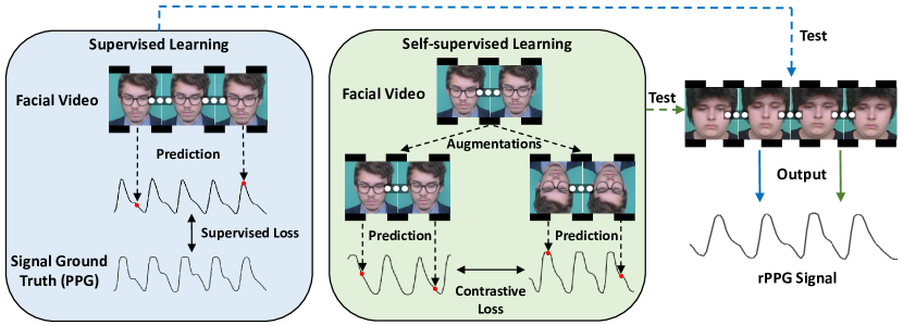
With the advent of deep learning [17], modern remote physiological measurement approaches train deep neural networks (DNNs) to estimate rPPG signals from facial videos [1, 3, 2, 15, 16, 4, 18, 19]. These methods are trained in a supervised manner, where PPG signals are recorded synchronously with facial videos for supervision (see Fig. 1). The collection of these annotated corpora is however not easy: subjects must wear skin-contact devices and keep body still to record both signals and videos. To bypass this process, Gideon et al. [20] have tried to train an rPPG estimator based on unlabeled data using contrastive learning. Contrastive learning normally treats multi-views of a given sample as positive samples, and other samples in the dataset as negative samples. Sample representations are optimized by pulling positive samples close and negative samples away in the feature embedding space. In this context, given an input video, Gideon et al. re-sample it with a pre-defined ratio to its negative counterpart, which has a different rPPG signal frequency. Positive and negative rPPG signals are respectively estimated from both the input and resampled videos. The contrastive loss is applied among these signals for model optimization. [20] is the first DNN-based self-supervised work for rPPG estimation. But it generates only one negative sample with a higher rPPG signal frequency to that of the input, which limits the sample diversity and can lead to inferior model generalizability.
In this paper, we propose a novel frequency-inspired self-supervised framework for facial video-based remote physiological measurement, which learns to optimize rPPG estimation from multiple augmented videos of different signal frequencies and across temporally neighboring videos of similar signal frequencies. It has three main stages: data augmentation, signal extraction and network optimization. Given an input video, in the first stage, we apply spatial augmentation (e.g. image rotation and flip) to obtain multiple positive samples, which contain rPPG signals with the same frequency to that of the input. Meanwhile, we design a learnable frequency augmentation (LFA) module to generate multiple negative samples which contain rPPG signals with different frequencies to that of the input. Unlike [20], our LFA module is integrated into the DNN for end-to-end training and produces multiple samples with controllable rPPG signal frequencies, which can be higher or lower than that of the input. In the second stage, because face is not an ideal Lambertian object, the distribution of blood vessels or noises varies over different regions in a face. Instead of treating face regions indiscriminately [2, 20], we design a local rPPG expert aggregation (REA) module to estimate rPPG signals from different face regions and aggregate them via a spatio-temporal gating net. The REA module is respectively devised for each augmented video sample (positive or negative) to obtain its rPPG signal. In the third stage, since we do not have ground truth PPG signals, we first introduce a frequency contrastive loss and a frequency ratio consistency loss to optimize our estimated rPPG signals. Furthermore, since the frequency of rPPG signal does not change rapidly over a short term, we additionally extract rPPG signals from multiple temporally neighboring videos to the input and introduce a cross-video frequency agreement loss for rPPG estimation across videos.
Overall, our new frequency-inspired self-supervised framework for remote physiological measurement has three key contributions:
-
1.
We design a learnable frequency augmentation module to generate sufficient and diverse negative samples for self-supervised learning.
-
2.
We introduce a local rPPG expert aggregation module to learn complementary information from different face regions for rPPG estimation.
-
3.
We propose a series of frequency-inspired losses (i.e. frequency contrastive loss, frequency ratio consistency loss, cross-video frequency agreement loss) for the optimization of rPPG signals extracted from the input’s augmentations and neighbors.
2 Related work
2.1 Remote physiological measurement
Facial video-based remote physiological measurement has been mainly implemented using blind signal separation [12, 25, 26], skin reflection models [9, 14], and deep neural networks [1, 3, 15]. First, blind signal separation-based approaches assume that the skin color change is a linear combination of the target rPPG signal and other noises. Signal decomposition methods, such as independent component analysis (ICA) or principal components analysis (PCA), are used to separate rPPG signals from noises. For example, Macwan et al. [25] used auto-correlation as a measurement for signal periodicity, so as to guide ICA for rPPG signal separation. McDuff et al. [26] leveraged ICA to estimate rPPG signals from multiple facial videos captured at different angles. Second, skin reflection model-based approaches explore different ways to project images from the RGB space to other color spaces for better rPPG estimation. For instance, Haan et al. [14] proposed to project images into the chrominance space to eliminate motion noises and help rPPG estimation. These approaches rely on assumptions, for instance, different people’s skin tones are identical under white light [14], which may not always be satisfied in a practical environment [15, 16]. We refer readers to [11] for a comprehensive and systematic survey on these traditional approaches.
Recently, DNN-based approaches have shown superior performance on remote physiological measurement [1, 3, 2, 15, 16, 4, 18, 19]. Hu et al. [27] designed a time-domain attention network to extract and aggregate temporal information from multiple video segments for rPPG estimation. Song et al. [15] transformed the chrominance signals in [14] into accurate rPPG waveforms using a conditional generative adversarial network. Yu et al. [18] and Yue et al. [2] respectively addressed rPPG estimation from highly compressed and low-resolution facial videos by adding video enhancement networks. Yu et al. [19] used transformer blocks to model the relationship among video frame features. Despite their remarkable achievements, these approaches need plenty of facial videos with synchronously recorded PPG signals for model training. The collection of these annotated corpora is however not easy. Gideon et al. [20] tackled this by training the DNN in a self-supervised manner using unlabelled data: they resampled the input video to create its negative counterpart and applied a contrastive loss among rPPG signals extracted from the input and resampled videos.
We propose a new frequency-inspired self-supervised framework for facial video-based remote physiological measurement. It differs from [20] significantly: 1) for data augmentation, [20] uses pre-processed video re-sampling to generate one negative sample, whose rPPG signal frequency can only be higher than that of the original sample. Our LEA module is instead learned to augment samples with arbitrary signal frequencies; 2) for signal extraction, [20] only captures image-level features and treats different face regions indiscriminately. Our REA module instead considers the pulsatile feature variance over face regions and advantageously aggregates their information for rPPG estimation; 3) for model optimization, [20] applies the contrastive loss among anchor, positive and negative rPPG signals. They all come from one video clip. We design a series of frequency-inspired losses; especially, the cross-video frequency agreement loss is proposed among rPPG signals extracted from multiple video clips.
It is worth noting that the three key contributions of our self-supervised framework are also unique among supervised methods in the remote physiological measurement.
2.2 Self-supervised learning
Self-supervised learning aims to learn an effective data embedding function from unlabelled data during training. Previous works focus on designing different pretext tasks to train the data encoders. For image encoders, solving jigsaw puzzles [28], rotation prediction [29] and counting primitives [30] are widely used tasks. For video encoders, predicting frames [31] and tracking patches [32] can help them learn useful feature representations. Recently, contrastive self-supervised learning attracts much attention and shows promising performance compared to supervised learning in both classification-based [33, 34, 35, 36, 37, 38] and regression-based tasks [39, 40, 41, 42]. Owing to the versatile data augmentation techniques, contrastive learning approaches augment the input into multiple positive counterparts, while considering other samples in the dataset as negatives to the input. They minimize feature distances between positive sample pairs while maximizing feature distances between negative sample pairs. For instance, SimCLR [33] leverages image cropping, color distortions and blurring to augment the input and applies contrastive learning. Dangovski et al. [41] proposed the equivariant contrastive learning, which utilizes an additional branch to predict the adopted augmentations of positive samples. Qian et al. [38] designed a novel temporal augmentation method for video representation learning, which samples non-overlapping positive video clips from the original video using different temporal intervals. Pan et al. [35] introduced another temporal augmentation method which obtains positive videos using a generate adversarial network. The network removes several frames from a given video while maintaining its spatio-temporal information. We realize the self-supervised video-based remote physiological measurement as a regression problem. Unlike the above approaches that use spatial or temporal augmentation, we propose a learnable frequency augmentation module to augment samples that contain different frequencies of rPPG signals.
2.3 Mixture of experts
Traditional mixture of experts (MoE) divides the input space into multiple sub-spaces and distributes them amongst multiple experts [43, 44]. A gating net is devised to assign soft or hard weights to experts to control their activations [43]. Zero coefficient problem usually occurs in traditional MoE [45]: because of the competition among experts, the gating net assigns near-zero weights to some of them due to their unfavourable initial parameters, which may lead to their elimination during training [46]. Moreover, the number of samples required for training traditional MoE scales up with the number of experts. Many modern MoE methods tend to extract information from different parts of a sample and combine their predictions via a gating net [47]. For example, Abdulhamit et al.[48] decomposed a given EEG signal into multiple frequency sub-bands using discrete wavelet transform; then predicted the probability of epilepsy from each frequency sub-band using a neural network; the outputs of different neural networks were combined via a gating net for the final diagnosis.
MoE has shown superior performance in many fields, such as image super-resolution [49], multi-modal/task learning [50, 51], and medical imaging [52]. For instance, Ma et al. [51] proposed a multi-gate MoE for multi-task learning. Experts capture task-shared representations while gating nets combine them using task-specific weights. Sahasrabudhe et al. [52] extracted information from blood smear images and patient clinical attributes (e.g. age and lymphocyte count) using a CNN and MLP model, respectively; they combined the outputs of two models via a gating net for the diagnosis of lymphocytosis. In this paper, we for the first time leverage multiple experts to estimate rPPG signals in different face regions and aggregate their complementary information via a spatio-temporal gating net.
3 Method
3.1 Overview
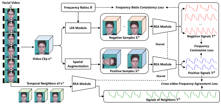
Our goal is to learn rPPG signals from unlabelled facial videos. The overview of our framework is illustrated in Fig. 2. The basic pipeline is to first generate positive and negative samples from the input video, then extract rPPG signals from them, and finally learn contrastive frequency information among these rPPG signals. Specifically, given a short facial video, we first follow [19, 53, 54] to use the open-source face detector MTCNN [55] to detect, align and crop the face area in each frame in advance. The face alignment operation in MTCNN aligns the upside-down faces, rotated faces, and even side faces to canonical frontal faces. Then we cut the aligned facial video into several clips, each with frames. One clip is randomly selected as the main input while the rest is taken as ’s temporal neighbors for later usage. In the data augmentation stage (Sec. 3.2), we first apply spatial augmentation to , which does not affect its interior rPPG signals, to generate a number of positive samples . Next, we introduce the learnable frequency augmentation (LFA) module to generate a number of negative samples which have different rPPG signal frequencies to that of . We feed a set of frequency ratios into the LFA module to modulate the rPPG signal of . Having and , in the signal extraction stage (Sec. 3.3), we pass them into local rPPG expert aggregation (REA) modules to estimate corresponding rPPG signals, denoted by and respectively. The REA module encodes complementary pulsation information from different face regions and uses a spatio-temporal gating net to aggregate the information for a final rPPG prediction. Last, in the network optimization stage (Sec. 3.4), the frequency contrastive loss is applied among signals from or between and . The frequency ratio consistency loss is applied between signals from and to enforce their frequency ratios according to input ratios in . We also introduce a cross-video frequency agreement loss by extracting rPPG signals from ’s temporal neighbors and enforcing their frequencies to be similar to that of .
3.2 Data augmentation: learnable frequency augmentation
Given the input video , we apply two different data augmentation strategies to generate positive and negative samples, respectively. For positive ones, we employ six spatial augmentation operations, i.e. image rotations (0°, 90°, 180°, and 270°), horizontal and vertical flips. They do not affect the interior rPPG signal of . Every time, we randomly select two operations to apply to and obtain two positive samples . They have the same rPPG signal frequency to that () of .
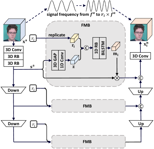
Next, we design a learnable frequency augmentation (LFA) module to generate multiple negative samples which contain rPPG signals with different frequencies to that of . Given the input of and a frequency ratio , it has a pyramid structure (see Fig. 3) to transform to a new sample with its rPPG signal frequency becoming . is a scalar randomly sampled from a predefined range, which represents the target frequency ratio upon which LFA modulates the original signal frequency. In the pyramid structure, we first use one 3D Convolution (Conv) layer followed by two 3D Res-blocks (3D RB) to extract the feature for and then down-sample it with a factor of 2 and 4 to obtain the multi-scale features. These features reflect different levels of details for . We modulate the frequency of rPPG signal on each scale via the frequency modulation block (FMB, see below Sec. 3.2.1). The modulated features are upsampled and concatenated. We reconstruct the video clip from the concatenated feature via one 3D Conv (). The reconstructed video clip is denoted by and is regarded as a negative sample to .
We know the frequency of human rPPG signal varies within a rather small range as a result of the human heart rate limit. On the one hand, we need to reinforce the module to change the rPPG signal frequency of to the target. On the other hand, we also make sure there is no excessive color difference between and , because, in reality, the face color changes caused by the blood volume variations are rather subtle. We develop the frequency ratio consistency loss (specified later in Sec. 3.4.2) and video reconstruction loss (see below Sec. 3.2.2) for the two purposes, respectively. Overall, during the training process, we randomly sample a set of frequency ratios within a range of and feed them into the LFA module to augment negative samples to , which should contain rPPG signals with frequencies of .
3.2.1 Frequency modulation block
The FMB, as illustrated in Fig. 3, takes the input of a certain scale feature and frequency ratio (scalar). is passed through a 3D global average pooling (3D GAP) to collapse its spatial dimensions and then a 1D Conv to collapse its channel dimensions, so as to obtain a rough rPPG signal . We aim to change the frequency of from to . Directly multiplying by only changes the signal amplitude but not the frequency. In practice, we replicate for times to create a vector and then concatenate it with . Their concatenation is processed via a 1D RB and a Bidirectional LSTM (BiLSTM). The Conv + ReLu in the 1D RB performs local transformation on the signal while the BiLSTM performs global transformation on it. This outputs a modulation vector , each of its entries can be seen as a multiplier to the corresponding component in , or equivalently corresponding frame in . We element-wisely multiply to to change its rPPG signal frequency from to . Note that, to obtain from the concatenation of and , the transformation needs to be non-linear (i.e. 1D RB and BiLSTM). This is due to the nature of signal frequency modulation. We give an example: assuming we have a periodic signal, , where , and denote the signal amplitude, frequency and shift, respectively. To modulate its frequency by a factor of 2, i.e. obtaining , we can compute the modulation vector as , which indicates a non-linear transformation. The experimental analysis between non-linear transformation and linear transformation is presented in Sec. 5.1.3.
3.2.2 Video reconstruction loss
According to [56], the pixel values vary within a very small range across frames in the facial video. Hence, we need to prevent the significant color change even between and its negative counterpart . This will also help the subsequent signal extractors (i.e. REA modules, Sec 3.3) to distinguish the positive and negative samples by their insignificant color differences, hence extract their accurate underlying rPPG signals. To cope with this problem, we can regulate either the modulation weight or the pixel-wise color distance between and to be small. The latter works empirically better than the former in our experiment (Sec. 5.1.4). We conceptualize the latter as the video reconstruction loss , which is indeed widely used in video frame inpainting [57] and video super-resolution [58], and write it out:
| (1) |
This loss enforces the LFA module to augment negative samples which retain the general visual appearance of .
3.3 Signal extraction: local rPPG expert aggregation

We extract the rPPG signal from each augmented sample via the local rPPG expert aggregation (REA) module. Our motivation is that different face regions have varying distributions of blood vessels and noises and should contribute differently to the rPPG estimation. Our REA module is designed to combine complementary pulsation information from these regions for accurate rPPG estimation.
The structure of the module is illustrated in Fig. 4a. We first leverage the 3D ResNet-10 [2] to encode the input video into a feature tensor. The feature tensor is then divided into evenly partitioned regions where we extract rPPG signal from each of them and denote it as a local rPPG expert . As illustrated in Fig. 4b, is obtained via two 3D RBs for feature processing; one region-attention block in-between the two 3D RBs for capturing physiological clues from pulsation-sensitive skins; and one 3D GAP followed by one 1D Conv for projecting the feature into 1D signal. Having for regions, we design a spatio-temporal gating net to aggregate different experts into one rPPG prediction.
Note that although the spatial augmentation we adopt for positive sample generation can change the spatial layout of face regions, we re-arrange the experts according to the same spatial augmentation to maintain the correspondence between the face regions and local rPPG experts. During testing, spatial augmentation is no longer used, we can directly connect face regions to their corresponding local rPPG experts.
Below we specify our region-attention block and spatio-temporal gating net.
3.3.1 Region-attention block
Within each face region, some pixels may belong to the background that do not contribute to rPPG estimation; while some other pixels, despite on the face, are insensitive to blood pulsation (e.g. eyes and mouth). Region-attention block is thereby introduced to focus rPPG estimation on the pulsation-sensitive skin area. Fig. 4b illustrates its structure: given the 4D input feature tensor (), after a 3D Conv, we leverage a 3D GAP to collapse it along the temporal dimension into a 3D tensor (). Inspired by the squeeze and excitation operation in [59], we pass the feature into consecutive 2D Conv and non-linear activation layers (i.e. ReLu, Sigmoid) for aggregating information across the channel dimension and obtaining the region-attention map. The attention map is pixel-wisely multiplied to the input 4D feature. A skip connection is also leveraged to retain the input information. Our scheme indeed transforms the image-based channel-wise attention in [59] into video-based spatial-wise attention, which enhances the pulsation-sensitive area and suppresses background and pulsation-insensitive area in rPPG estimation. The superiority of the proposed region-attention block is experimentally demonstrated in Sec. 5.2.1.
3.3.2 Spatio-temporal gating net
The idea of employing a gating net to combine experts is from mixture of experts [43]. The conventional design of gating net [49, 52] normally assigns sample-level weights among experts. Unlike them, we introduce the spatio-temporal gating net which assigns spatio-temporal weights to combine temporal rPPG signals (experts) extracted from different spatial regions. Our motivation is that some regions may reflect rPPG signal better during the systole while some are more sensitive during the diastole. Each expert signal should be assigned with different weights at different moments. The structure of is illustrated in Fig. 4a, consisting of two 3D Convs followed by a Reshape, a 3D GAP, a 1D Conv and a Softmax layer, respectively. The gating net generates vectors, , , , corresponding to experts . Each vector is of dimension , equivalent to the temporal dimension of each expert. Vector components of the same index are softmaxed across experts, i.e. , to ensure that, at the -th moment, the sum of weights assigned to all experts to be 1. We element-wisely multiply each to its corresponding and obtain the final rPPG signal as a weighted combination:
| (2) |
The REA module is devised for positive and negative video samples to produce positive signals and negative signals . These signals are of various frequencies and can be used for subsequent self-supervised training.
3.4 Network optimization: frequency-inspired losses
We introduce a series of frequency-inspired losses, i.e. frequency contrastive loss, frequency ratio consistency loss, cross-video frequency agreement loss, for the optimization of rPPG signals generated from the input video’s augmentations and neighbors.
3.4.1 Frequency contrastive loss
Since we do not have ground truth PPG signals for training, we use the popular contrastive self-supervised learning [60, 34] to pull close rPPG signals () from positive samples while pushing them away from rPPG signals () from negative samples in the feature space. We adapt the InfoNCE loss [60] to write out our frequency contrastive loss :
| (3) |
where measures the frequency difference between two signals and is the temperature. We follow [20] to realize as the mean squared error between power spectral densities (PSD) of two signals. PSD describes the power of different frequency components in a signal. Notice [20] utilizes the triplet loss to optimize among only three signals, i.e. anchor, positive and negative; we have a different loss form as a result of our larger numbers of positive and negative signals generated by different ways.
3.4.2 Frequency ratio consistency loss
This loss constrains that the frequency ratio between any positive and negative rPPG signals ( and ) should be consistent with the corresponding ratio fed into the LFA module. It optimizes the LFA module to generate a certain negative sample with the target signal frequency. We define the frequency ratio consistency loss :
| (4) |
where we use to measure a signal’s dominant frequency. is implemented by following [13] to apply the fast Fourier transform on a given signal and select the frequency component with maximum power. and should ideally have the same frequency. indicates the dominant frequency ratio between signal and . If this ratio is equal to , that means the LFA module has successfully generated with the target rPPG signal frequency .
3.4.3 Cross-video frequency agreement loss
This loss function is built upon the observation that the frequency of an rPPG signal does not change rapidly over a short term. Based on this, the rPPG signal from the input should have a similar frequency to those from ’s temporal neighbors (see Sec. 3.1). We pass ’s neighboring video clips through REA modules to extract rPPG signals from them, i.e. . We design the cross-video frequency agreement loss to enforce the frequency conformability between and :
| (5) |
where is the same to that in Eqn. 3. We have neighbors in total. This loss helps reduce the signal estimation error and improve the signal periodicity.
4 Experiments
4.1 Datasets
We conduct our experiments on five public datasets: UBFC-rPPG [21], PURE [22], DEAP [23], MMVS [2], and BP4D+ [24].
UBFC-rPPG consists of 42 facial videos with simultaneously recorded PPG signals and heart rates. The resolution and frame rate of each facial video is and 30 frames per second (FPS), respectively. We follow [3] to discard subjects of indices 11, 18, 20 and 24 because their heart rates were inappropriately recorded.
PURE contains 60 facial videos from 10 subjects. During the data collection process, subjects were asked to perform six kinds of head motions (small rotation, medium rotation, slow translation, fast translation, talking and steady) in front of the camera for one minute. The videos were captured at a frame rate of 30 FPS and a resolution of . The ground truth PPG signals were recorded using a finger clip pulse oximeter with a sampling rate of 60 Hz. We follow [20] to discard the first two samples because their PPG waveforms were strongly corrupted.
DEAP consists of 874 facial videos associated with multi-channel physiological signals. They were taken from 22 subjects by playing one-minute musical excerpts to them. Each facial video has a resolution of and a frame rate of 50 FPS.
MMVS contains 745 facial videos from 129 subjects. A depth camera and a finger clip pulse oximeter was utilized to record facial videos and PPG signals, respectively. The resolution of each captured video is and the frame rate is 25 FPS. The sampling rate for PPG signals is 60 Hz.
BP4D+ contains 548 facial videos from 140 subjects. There are 58 male subjects and 82 female subjects, with their ages ranging from 18 to 66. Ethnicities of these subjects include Caucasian, African and Asian (East-Asian and Middle-East-Asian); specifically, 64 Caucasian, 46 Asian, and 15 African subjects. The resolution and frame rate of each video is and 25 FPS, respectively.
4.2 Implementation Details
For facial videos in five datasets, we randomly sample consecutive 600 frames from each video and follow [20] to scale them into a resolution of for training. We cut the 600-frame video into four clips, each with an equivalent length of 150 frames. In every iteration, we randomly select one clip as the main input while the rest three ( in Eqn. 5) are its neighbors. The number of negative samples, , is set to 4. The number of face regions, , is set to 9. The temperature in Eqn. 3 is set to 0.08. Most parameter settings in this paper follow the common practices in the literature. For instance, is equivalent to that in [61]; is inspired by [19]; is the same to that in [62]; while and are equivalent to that in [19] and [63], respectively.
Our model is trained for 100 epochs on four NVIDIA GeForce RTX 2080 GPUs using Pytorch 1.8.0. We use the Adam [64] optimizer and set the batch size to 4. The learning rate is initialized as and is decreased to at the 50-th epoch.
4.3 Evaluation Protocol
Previous works calculate the heart rate (HR), heart rate variability (HRV) and respiration frequency (RF) from estimated rPPG signals and compare them to the corresponding ground truth for performance evaluation [4, 15, 16, 18]. We follow them to conduct HR evaluation on five datasets; HRV and RF evaluation on the UBFC-rPPG dataset. Moreover, we perform cross-dataset HR evaluation among UBFC-rPPG, PURE and MMVS. The calculation of HR, HRV and RF is via the toolkit HeartPy [65].
We follow [15, 20] to use mean absolute error (MAE), root mean square error (RMSE) and Pearson’s correlation coefficient () as evaluation metrics for HR. For HRV, we follow [4, 19, 16] to compute its three attributes, i.e. low frequency (LF), high frequency (HF), and LF/HF ratio. LF and HF are calculated from the interbeat intervals under low frequency (0.04 to 0.15 Hz) and high frequency (0.15 to 0.4 Hz) bands of the rPPG signal [19, 4]. For each attribute of HRV, we report the standard deviation (Std) of estimation errors, RMSE and . Finally, for RF, we also report the Std, RMSE and as per most comparable methods [4, 16, 18]. We follow [2, 4, 16] to perform the 5-fold subject-exclusive cross-validation for all experiments.
| Method | PPG | UBFC-rPPG | PURE | DEAP | MMVS | BP4D+ | ||||||||||
|---|---|---|---|---|---|---|---|---|---|---|---|---|---|---|---|---|
| annotations | MAE | RMSE | MAE | RMSE | MAE | RMSE | MAE | RMSE | MAE | RMSE | ||||||
| POS [9] | - | 8.35 | 10.00 | 0.24 | 3.14 | 10.57 | 0.95 | 7.39 | 10.25 | 0.82 | 6.77 | 9.40 | 0.82 | 6.82 | 9.70 | 0.77 |
| CHROM [14] | - | 8.20 | 9.92 | 0.27 | 3.82 | 6.80 | 0.97 | 7.47 | 10.31 | 0.82 | 6.85 | 9.37 | 0.82 | 7.25 | 9.91 | 0.72 |
| Green [66] | - | 6.01 | 7.87 | 0.29 | 4.39 | 11.60 | 0.90 | 8.10 | 11.17 | 0.80 | 7.13 | 9.46 | 0.80 | 6.76 | 9.73 | 0.76 |
| SynRhythm [67] | 5.59 | 6.82 | 0.72 | 2.71 | 4.86 | 0.98 | 5.08 | 5.92 | 0.87 | 4.48 | 6.52 | 0.89 | 4.33 | 6.15 | 0.85 | |
| Meta-rppg [3] | 5.97 | 7.42 | 0.53 | 2.52 | 4.63 | 0.98 | 5.16 | 6.00 | 0.87 | 4.30 | 6.20 | 0.91 | 4.08 | 6.11 | 0.86 | |
| PulseGan [15] | 1.19 | 2.10 | 0.98 | 2.28 | 4.29 | 0.99 | 4.86 | 5.70 | 0.88 | 3.52 | 5.09 | 0.93 | 3.84 | 5.37 | 0.89 | |
| Dual-Gan [4] | 0.44 | 0.67 | 0.99 | 0.82 | 1.31 | 0.99 | 3.25 | 4.11 | 0.91 | 3.00 | 4.27 | 0.94 | 2.96 | 4.18 | 0.93 | |
| Physformer [19] | 0.40 | 0.71 | 0.99 | 1.10 | 1.75 | 0.99 | 3.03 | 3.96 | 0.92 | 3.28 | 4.50 | 0.93 | 3.10 | 4.33 | 0.92 | |
| Gideon et al. [20] | 1.85 | 4.28 | 0.93 | 2.32 | 2.97 | 0.99 | 5.13 | 6.16 | 0.86 | 3.43 | 4.74 | 0.93 | 4.09 | 5.60 | 0.85 | |
| Ours | 0.58 | 0.94 | 0.99 | 1.23 | 2.01 | 0.99 | 4.20 | 5.18 | 0.90 | 2.93 | 4.16 | 0.94 | 3.22 | 4.47 | 0.91 | |
4.4 Results
4.4.1 HR evaluation
We first evaluate the HR estimation on five datasets. Representative approaches include: 1) traditional blind signal separation- and skin reflection model-based ones: POS [9], CHROM [14] and Green [66]; 2) modern DNN-based supervised ones: SynRhythm [67], Meta-rppg [3], PulseGan [15], Dual-Gan [4], Physformer [19]; and 3) a recent DNN-based self-supervised one: Gideon et al. [20]. Their results are shown in Table I.
First, we observe that the performance of traditional approaches [9, 14, 66] is much inferior to DNN-based ones. DNN-based approaches can be trained in a data-driven way, while traditional approaches heavily rely on priors, which can not always satisfy. Second, DNN-based self-supervised approaches ([20] and ours) show comparable performance to many supervised ones, e.g. [67, 3, 15, 4, 19].
Our approach outperforms many supervised approaches. For instance, on the MMVS dataset, it even decreases the MAE/RMSE from best performing one Dual-Gan [4] by 0.07/0.11. MMVS is a large-scale dataset in which videos were captured from different scenarios. We reproduce the state of the art on MMVS using their default parameters, which may need to be adjusted on this large-scale dataset. In contrast, our self-supervised model has demonstrated good generalizability on this dataset.
Our model also significantly outperforms the very recent self-supervised approach Gideon et al. [20] on all five datasets; for example, on UBFC-rPPG, it decreases MAE by 1.27 and RMSE by 3.34. This justifies the effectiveness of our proposed modules and losses.

It is worth noting that the general performance of comparable methods on the DEAP dataset is clearly inferior to that on the rest datasets. The reason is that, during the data collection process of the DEAP dataset, subjects wore many devices on their heads to record multi-channel physiological signals, such as EEG, EOG and EMG signals. Devices like EEG caps, electrodes and wires on the heads cover many skin areas, thus hindering the capturing of physiological clues for rPPG estimation. While subjects in other datasets did not wear these devices. Some face images in UBFC-rPPG, MMVS and DEAP datasets are shown in Fig. 5.
| PPG | RF | HRV: LF | HRV: HF | HRV: LF/HF | |||||||||
|---|---|---|---|---|---|---|---|---|---|---|---|---|---|
| annotations | Std | RMSE | Std | RMSE | Std | RMSE | Std | RMSE | |||||
| POS [9] | - | 0.109 | 0.107 | 0.087 | 0.171 | 0.169 | 0.479 | 0.171 | 0.169 | 0.479 | 0.405 | 0.399 | 0.518 |
| CHROM [14] | - | 0.086 | 0.089 | 0.102 | 0.243 | 0.240 | 0.159 | 0.243 | 0.240 | 0.159 | 0.655 | 0.645 | 0.266 |
| Green [66] | - | 0.087 | 0.086 | 0.111 | 0.186 | 0.186 | 0.280 | 0.186 | 0.186 | 0.280 | 0.361 | 0.365 | 0.492 |
| CVD [16] | 0.017 | 0.018 | 0.252 | 0.053 | 0.065 | 0.740 | 0.053 | 0.065 | 0.740 | 0.169 | 0.168 | 0.812 | |
| rPPGNet [18] | 0.030 | 0.034 | 0.233 | 0.071 | 0.070 | 0.686 | 0.071 | 0.070 | 0.686 | 0.212 | 0.208 | 0.744 | |
| Dual-Gan [4] | 0.010 | 0.010 | 0.395 | 0.034 | 0.035 | 0.891 | 0.034 | 0.035 | 0.891 | 0.131 | 0.136 | 0.881 | |
| Physformer [19] | 0.009 | 0.009 | 0.413 | 0.030 | 0.032 | 0.895 | 0.030 | 0.032 | 0.895 | 0.126 | 0.130 | 0.893 | |
| Gideon et al. [20] | 0.061 | 0.098 | 0.103 | 0.091 | 0.139 | 0.694 | 0.091 | 0.139 | 0.694 | 0.525 | 0.691 | 0.684 | |
| Ours | 0.023 | 0.028 | 0.351 | 0.047 | 0.062 | 0.769 | 0.047 | 0.062 | 0.769 | 0.160 | 0.164 | 0.831 | |
| Method | PPG annotations | MMVSUBFC-rPPG | UBFC-rPPGMMVS | PUREUBFC-rPPG | UBFC-rPPGPURE | ||||||||
|---|---|---|---|---|---|---|---|---|---|---|---|---|---|
| MAE | RMSE | MAE | RMSE | MAE | RMSE | MAE | RMSE | ||||||
| Meta-rppg [3] | 6.48 | 7.97 | 0.52 | 5.69 | 7.74 | 0.84 | 6.11 | 7.58 | 0.66 | 4.00 | 5.98 | 0.92 | |
| PulseGan [15] | 2.33 | 3.62 | 0.97 | 4.40 | 6.35 | 0.89 | 2.30 | 3.50 | 0.97 | 3.36 | 5.11 | 0.95 | |
| Dual-Gan [4] | 2.00 | 3.13 | 0.97 | 3.51 | 4.99 | 0.93 | 2.03 | 3.01 | 0.97 | 1.81 | 2.97 | 0.99 | |
| Physformer [19] | 1.97 | 3.08 | 0.97 | 3.46 | 4.96 | 0.93 | 1.93 | 3.02 | 0.97 | 1.99 | 3.28 | 0.99 | |
| Gideon et al. [20] | 2.45 | 3.71 | 0.93 | 3.84 | 5.31 | 0.91 | 2.37 | 3.51 | 0.95 | 2.95 | 4.60 | 0.97 | |
| Ours | 2.24 | 3.40 | 0.97 | 3.50 | 4.95 | 0.93 | 2.18 | 3.20 | 0.97 | 2.14 | 3.37 | 0.98 | |
 |
 |
| (a) | (b) |
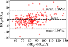
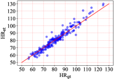
Fig. 6 shows the Bland-Altman plot and scatter plot on the MMVS dataset. HR and HR represent the HR calculated from the ground truth PPG signal and the estimated rPPG signal, respectively. Each point indicates an estimation result from one test sample. The x-axis in the Bland-Altman plot denotes the mean value of HR and HR while the y-axis represents their difference. The top and bottom dashed lines indicate confidence intervals for 95% limits of agreement. We can observe that HR is well correlated with HR within a wide range from 50 bpm to 130 bpm. The Pearson’s correlation coefficient between HR and HR of our approach is 0.94 (Fig. 6b), which is higher than that of other methods, e.g. Meta-rppg [3] (0.91), PulseGan [15] (0.93), Physformer [19] (0.93), Gideon et al. [20] (0.93).
4.4.2 RF and HRV evaluation
 |
 |
 |
 |
We further conduct experiments for RF and HRV estimation on the UBFC-rPPG dataset. As mentioned in Sec. 4.3, HRV is represented by its three attributes (LF, HF, LF/HF). Similar to the HR evaluation, we compare our approach with state of the art [9, 14, 66, 16, 18, 4, 19, 20]. The results are shown in Table II. We can see that our approach outperforms all traditional ones and many deep learning ones. For example, as a self-supervised method, we have a comparable performance with the very recent supervised method Physformer [19]; moreover, we outperform the self-supervised competitor [20] by large margins on all metrics.
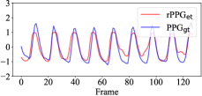
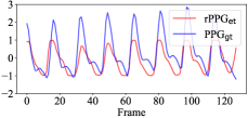
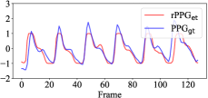
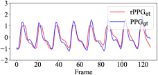
Fig. 7 shows four estimated rPPG signals and their corresponding ground truth. We can observe that our method predicts rPPG signals with very accurate interbeat intervals compared to ground truth, from which we can obtain robust RF and HRV results.
4.4.3 Cross-dataset HR evaluation
To evaluate the generalizability of our method, we conduct the cross-dataset experiment among UBFC-rPPG, PURE and MMVS datasets and report the HR estimation results in Table III. Specifically, we train our model, as well as state of the art, i.e. [3, 15, 4, 19, 20], on one dataset and test them on another. For example, MMVSUBFC-rPPG means training on MMVS while testing on UBFC-rPPG. Ours and [20] are trained in the self-supervised way while the rests are in the supervised way. The parameter settings for cross-dataset experiments remain the same to original intra-dataset experiments. We can see that our method produces very competitive results on par with state of the art supervised methods [15, 4, 19]; significantly outperforms the recent self-supervised method [20]. This shows the good generalizability of our method in new (unseen) scenarios.
5 Ablation study
| Method | UBFC-rPPG | MMVS | ||||
|---|---|---|---|---|---|---|
| MAE | RMSE | MAE | RMSE | |||
| Ours | 0.58 | 0.94 | 0.99 | 2.93 | 4.16 | 0.94 |
| LFAVSH | 1.27 | 1.91 | 0.97 | 3.21 | 4.48 | 0.93 |
| LFAVST [68] | 0.91 | 1.55 | 0.97 | 3.09 | 4.35 | 0.93 |
| LFAVST [69] | 0.82 | 1.40 | 0.98 | 3.09 | 4.33 | 0.93 |
| FMB-Linear | 1.05 | 1.71 | 0.97 | 3.17 | 4.46 | 0.93 |
| FMB w/o 1D RB | 0.80 | 1.30 | 0.98 | 3.03 | 4.39 | 0.93 |
| FMB w/o BiLSTM | 0.72 | 1.25 | 0.99 | 3.00 | 4.29 | 0.93 |
| FMB-LSTM | 0.66 | 1.07 | 0.99 | 2.98 | 4.26 | 0.94 |
| FMB-GRU | 0.68 | 1.06 | 0.99 | 2.98 | 4.26 | 0.94 |
| FMB-BiGRU | 0.60 | 0.97 | 0.99 | 2.93 | 4.19 | 0.94 |
| LFA w/o | 0.88 | 1.36 | 0.98 | 3.04 | 4.34 | 0.94 |
| 0.69 | 1.11 | 0.99 | 3.02 | 4.30 | 0.93 | |
We conduct ablation study from five aspects: LFA module, REA module, frequency-inspired losses, temporally neighboring videos and spatial augmentation. The results for HR estimation are reported on UBFC-rPPG and MMVS datasets.
5.1 Learnable frequency augmentation (LFA) module
5.1.1 LFA v.s. video shrinking/stretching
Table IV presents the ablation study on the proposed LFA module. Instead of learning to generate negative samples in the network, we can also leverage video shrinking (VSH) and video stretching (VST) to achieve this. We use LFAVSH and LFAVST to indicate the two variants in Table IV and compare them to our LFA.
Specifically, for video shrinking, we follow [20] to reduce the frame number of the input video and generate one negative sample; for video stretching, the most common way is through video frame interpolation; we select two state of the art video frame interpolation methods, i.e. Bilateral Motion Estimation with Bilateral Cost Volume (BMBC) [68] and Asymmetric Bilateral Motion Estimation (ABME) [69], to respectively stretch the video and generate negative samples.
In Table IV, we can observe severe performance degradation by replacing LFA with VSH or VST. The reason is two-fold: 1) in LFAVSH, the frame number of the shrunk video will be less than that of the original video, which means the number of sampling points of the extracted rPPG signal will also be reduced. Insufficient number of sampling points in the signal can bring in spurious components on the power spectral PSD analysis [70], which is not desired as we need precise PSD in our frequency-inspired losses; 2) in LFAVST, the rPPG signal frequency of the stretched video can only be lower than that of the original video (the number of signal waves per unit of time is decreased). This would lead to poor signal frequency diversity, hence impeding the model training. Besides, the majority of video interpolation methods pay more attention to recovering smooth motions than restoring skin color changes. The original periodicity or quasi-periodicity of rPPG waveforms is likely to be destroyed after adopting the video interpolation methods. Overall, video shrinking/stretching is not a good option for generating negative samples.
| Method | UBFC-rPPG | MMVS | ||||
|---|---|---|---|---|---|---|
| MAE | RMSE | MAE | RMSE | |||
| LFA-S1 | 0.83 | 1.32 | 0.98 | 3.04 | 4.33 | 0.94 |
| LFA-S2 | 0.66 | 1.06 | 0.99 | 2.99 | 4.24 | 0.94 |
| LFA-S3 | 0.58 | 0.94 | 0.99 | 2.93 | 4.16 | 0.94 |
| LFA-S4 | 0.58 | 0.95 | 0.99 | 2.96 | 4.15 | 0.94 |
5.1.2 Multi-scale in LFA
The LFA module performs frequency transformation on three scales (S3). We also experiment with one scale (S1), two scales (S2) and four scales (S4) in Table V. They are denoted as LFA-S1, LFA-S2 and LFA-S4, respectively. We can observe that LFA-S3 performs in general the best. LFA-S4 performs very close to LFA-S3 yet with additional computation. LFA-S1/S2 performs clearly inferior to LFA-S3. Overall, the three-scale version appears to be sufficient to describe different levels of details for the input. This is our default setting.
5.1.3 Feature modulation block in LFA
We further verify the design of the feature modulation block (FMB) in the LFA module. As mentioned in Sec. 3.2.1, the key part of FMB is the 1D RB and BiLSTM for non-linear signal frequency transformation. A linear transformation is not adequate. For instance, we can replace 1D RB + BiLSTM with three 1D Convs, which we call it FMB-Linear in Table IV. We see that the performance drops substantially by FMB-Linear, attesting that non-linear functions are important for frequency transformation.
Furthermore, we use FMB w/o 1D RB and FMB w/o BiLSTM to denote the FMB without 1D RB or BiLSTM. We can observe that both 1D RB and BiLSTM contribute to the final result. 1D RB is responsible for the signal’s local transformation followed by a non-linear activation function (ReLu). BiLSTM dedicates to the signal’s global transformation along the temporal dimension. Alternatively, we can replace BiLSTM with other RNN units, such as LSTM, GRU and BiGRU. We name these variants as FMB-LSTM, FMB-GRU and FMB-BiGRU in Table IV: they show competitive performance but our FMB with BiLSTM is the best.
5.1.4 Video reconstruction loss in LFA
We utilize video reconstruction loss to reduce color differences between negative samples and the original sample. If we remove , the result (LFA w/o in Table IV) will be much inferior. As mentioned in Sec. 3.2.2, an alternative to is to regulate the modulation vector, i.e. . We report the result for this variant in Table IV: , it works by improving upon LFA w/o yet it is no better than Ours with .
5.1.5 Number of negative samples in LFA
In the training phase, we found that the number of negative samples affects the model performance. We vary this number from 1 to 6 and report the result in Table VI. Our default setting () appears to be the best.
| Method | UBFC-rPPG | MMVS | ||||
|---|---|---|---|---|---|---|
| MAE | RMSE | MAE | RMSE | |||
| Ours () | 1.10 | 1.87 | 0.97 | 3.10 | 4.28 | 0.93 |
| Ours () | 1.03 | 1.66 | 0.97 | 3.07 | 4.35 | 0.94 |
| Ours () | 0.75 | 1.27 | 0.98 | 3.00 | 4.23 | 0.94 |
| Ours () | 0.58 | 0.94 | 0.99 | 2.93 | 4.16 | 0.94 |
| Ours () | 0.58 | 0.96 | 0.99 | 2.93 | 4.15 | 0.94 |
| Ours () | 0.59 | 0.92 | 0.99 | 2.96 | 4.15 | 0.94 |
| Method | UBFC-rPPG | MMVS | ||||
|---|---|---|---|---|---|---|
| MAE | RMSE | MAE | RMSE | |||
| Ours | 0.58 | 0.94 | 0.99 | 2.93 | 4.16 | 0.94 |
| REAGRA | 1.16 | 1.85 | 0.97 | 3.29 | 4.61 | 0.93 |
| REA w/o RA | 1.02 | 1.69 | 0.97 | 3.13 | 4.40 | 0.93 |
| RASA | 0.62 | 0.95 | 0.99 | 2.96 | 4.22 | 0.94 |
| 1.12 | 1.89 | 0.97 | 3.23 | 4.56 | 0.93 | |
| 0.76 | 1.26 | 0.98 | 3.07 | 4.41 | 0.94 | |
| Method | UBFC-rPPG | MMVS | ||||
|---|---|---|---|---|---|---|
| MAE | RMSE | MAE | RMSE | |||
| Ours () | 0.75 | 1.15 | 0.98 | 3.17 | 4.48 | 0.93 |
| Ours () | 0.61 | 0.98 | 0.99 | 2.97 | 4.19 | 0.94 |
| Ours () | 0.58 | 0.94 | 0.99 | 2.93 | 4.16 | 0.94 |
| Ours () | 0.57 | 0.94 | 0.99 | 2.95 | 4.16 | 0.94 |
| Ours () | 0.58 | 0.95 | 0.99 | 2.94 | 4.18 | 0.94 |
5.2 Local rPPG expert aggregation (REA) module
We investigate the effectiveness of the REA module in Table VII. The first variant is to not use the local rPPG experts but simply extract the rPPG signal from the entire face. The REA module degrades to one 3D ResNet-10 block at the beginning followed by one 3D GAP and one 1D Conv for rPPG estimation. We denote this variant as a global rPPG estimation (GRA) module, i.e. REAGRA, in Table VII. We can observe that the MAE increases by 0.58 and the RMSE increases by 0.91 on UBFC-rPPG. This shows that encoding complementary pulsation information from different face regions helps improve the rPPG estimation. Below we study the importance of the region-attention (RA) block and spatio-temporal gating net in the REA module.
5.2.1 Region-attention block in REA
Referring to Fig. 4b, we can replace the RA block with a 3D RB in the REA module. We denote this by REA w/o RA in Table VII: the MAE increases to 1.02, RMSE increases to 1.69, and decreases to 0.97 on the UBFC-rPPG dataset. The proposed RA block is more effective than a simple 3D RB in finding the pulsation-sensitive area in a local region. Alternatively, we follow [18] to use an additional skin segmentation branch after the 3D ResNet-10 block. This branch produces a seg-attention (SA) map, which we use to replace our region-attention map and is multiplied back to the encoded feature. We denote this by RA SA. It performs better than REA w/o RA but is still inferior to RA. SA map assigns weights to pixels according to their likelihood of being face skins; our RA map instead assigns weights to pixels according to their sensitivities to pulsation changes. RA can capture more discriminative physiological clues from face skins for rPPG estimation.
5.2.2 Spatio-temporal gating net in REA
The spatio-temporal gating net assigns weights to local rPPG experts for their aggregation. If we remove it from the REA module but take the average of multiple experts, the MAE and RMSE will be significantly increased for HR estimation (see Table VII: ). This supports our claim that the distribution of blood vessels varies over face regions. Our gating net treats these regions differently in rPPG estimation. Next, we adjust to assign one scalar weight to one expert (corresponding to a spatial region) while ignoring the temporal change in the signal. We denote this by in Table VII: one can clearly see the performance drop by this variant. This validates our motivation that each expert signal should be assigned different weights at different moments (see Sec. 3.3.2).
5.2.3 Number of experts in REA
We vary the number of local rPPG experts from 2, 4 (), 9 (), 16 (), and 25 () in the REA module and show the performance in Table VIII. Our default setting () appears to be the best. Yet, the performance difference for from 4 to 25 is not big.
| Method | UBFC-rPPG | MMVS | ||||
|---|---|---|---|---|---|---|
| MAE | RMSE | MAE | RMSE | |||
| Ours | 0.58 | 0.94 | 0.99 | 2.93 | 4.16 | 0.94 |
| Ours w/o | 2.13 | 3.09 | 0.83 | 5.00 | 6.74 | 0.85 |
| Ours w/o | 0.89 | 1.39 | 0.98 | 3.07 | 4.35 | 0.94 |
| Ours w/o | 0.67 | 1.08 | 0.99 | 3.04 | 4.30 | 0.94 |
| 0.66 | 1.08 | 0.99 | 3.00 | 4.24 | 0.94 | |
| 0.60 | 0.98 | 0.99 | 3.00 | 4.26 | 0.94 | |
| Ours-expand | 0.55 | 0.96 | 0.99 | 2.94 | 4.14 | 0.94 |
5.3 Frequency-inspired losses
To validate the effectiveness of our proposed frequency contrastive loss , frequency ratio consistency loss , cross-video frequency agreement loss , we ablate them one by one in our framework and show the results in Table IX. We observe a clear performance drop by removing any of them.
5.3.1 Frequency contrastive loss
Without using , the MAE and RMSE for HR evaluation are substantially increased while is substantially decreased, e.g. 5.00, 6.74 and 0.85 on MMVS. enforces the signal frequency similarities among positive samples and dissimilarities between positive and negative samples. It optimizes the model embedding space to be discriminative to skin color changes.
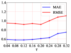
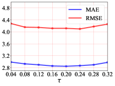
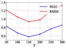
We further vary the temperature parameter in from 0.04 to 0.32 to explore its influence on the model performance. The MAE and RMSE on HR estimation are shown in Fig. 8. We can observe that, for both datasets, the performance of our default setting of is close to the best, and also does not fluctuate much in the neighborhood. Hence, we recommend sticking with the default setting for the sake of model’s generalizability. The temperature plays a role in controlling the strength of penalties on hard negative samples [71]. A small temperature tends to penalize more on hard samples. In Fig. 8 we can see that the best on the MMVS dataset is bigger than that of UBFC-rPPG. This is consistent with our experimental finding in Table I: results on UBFC-rPPG are generally better than on MMVS. This indicates UBFC-rPPG is an easier dataset compared to MMVS. A small temperature on UBFC-rPPG will focus the model on distinguishing hard negative samples. While for MMVS, a large temperature is more suitable to let the model distinguish the majority of negative samples as they are already quite difficult.
 |
 |
| (a) UBFC-rPPG | (b) MMVS |
 |
 |
| (a) UBFC-rPPG | (b) MMVS |
 |
 |
| (a) UBFC-rPPG | (b) MMVS |
5.3.2 Frequency ratio consistency loss
Without , the result also gets worse on both UBFC-rPPG and MMVS datasets. consists of two terms corresponding to the two positive signals, and , which should ideally share the same frequency. Nonetheless, we argue that in practice both and are important in Eqn.4. We offer a variant by keeping only the first term in Eqn.4 and name it as in Table IX. This shows inferior performance compared to the original (Ours). Having both terms in Eqn.4 can implicitly pull the two positive signals close.
5.3.3 Cross-video frequency agreement loss
We conduct a similar experiment to that of by removing , where a clear performance drop can be observed on both datasets. Next, we offer a variant of by keeping only its first term in Eqn.5. We denote this by in Table IX. The result also gets worse, which further validates the importance of having both positive signals.
5.4 Temporally neighboring videos
Given a short facial video, we cut it into clips, each with frames, and randomly select one as the main input . In this session, we study the attributes of these temporal neighbors.
5.4.1 Number of video clips
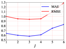
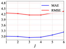
We vary the number of video clips while fixing the length of each clip to 150. We vary from 1 to 6 in Fig. 9. We only draw the MSE and RMSE results on HR estimation; the change for Pearson coefficient is insignificant. We can see the performance is stable on both datasets between and 4. In general, we argue that should not be too big; otherwise, the signals from temporal neighbors would not be similar. Our default is 3.
5.4.2 Length of one video clip
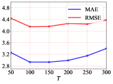
We also vary the length of each video clip from 50, 100, 150, 200, 250, and 300 in Fig. 10. The number of video clips is fixed to 4 (). We can observe that appears to be the best on UBFC-rPPG. The performance on MMVS is rather stable by varying between 100 and 200. Similar to , should also not be too big such that neighboring signals remain to be similar.
5.4.3 Augmentation
We notice that for ’s neighbors, they are only applied with the loss , but are not augmented and applied with other losses (, , ). This is because the rPPG signals among neighboring video clips are very similar, there is no need to repeat the augmentation process for every one of them. To support our claim, we apply all loss terms to both and its neighbors, and denote this by Ours-expand in Table IX. Only slight improvement can be observed by comparing it to Ours. Considering the computation increase, we do not recommend it.
| Method | UBFC-rPPG | MMVS | ||||
|---|---|---|---|---|---|---|
| MAE | RMSE | MAE | RMSE | |||
| Ours () | 0.62 | 1.00 | 0.99 | 2.95 | 4.20 | 0.94 |
| Ours () | 0.58 | 0.94 | 0.99 | 2.93 | 4.16 | 0.94 |
| Ours () | 0.58 | 0.95 | 0.99 | 2.93 | 4.15 | 0.94 |
| Ours () | 0.56 | 0.96 | 0.99 | 2.94 | 4.16 | 0.94 |
| Ours-CJ | 7.33 | 8.97 | 0.20 | 8.29 | 10.98 | 0.47 |
| Ours-SF | 7.59 | 9.55 | 0.19 | 8.33 | 10.70 | 0.46 |
5.5 Spatial Augmentation
We investigate the number of spatially augmented samples and the type of spatial augmentation.
5.5.1 The number of spatially augmented samples
We vary the number of positive (spatially augmented) samples from to in Table X. When the number is 2, it appears to be a good trade-off between accuracy and computation. This is also our default setting. Notice that [20] only generates one positive sample by applying inverse transformation on the negative one, which is fundamentally different from our spatial augmentation.
5.5.2 The type of spatial augmentation
The spatial augmentation we adopt includes image rotation and flip. We choose them because they do not alter the colors across frames, thus do not affect the rPPG signals contained in videos. There exist many other types of spatial augmentation, e.g. color jittering and Sobel filtering. They are however not suitable for our task, as they clearly alter the color distribution across frames, so as to change the underlying signal frequencies in videos. To validate this, we offer two variants, denoted by Ours-CJ and Ours-SF, in Table X. For each variant, we generate two positive samples, one is the original input, the other is with color jittering or Sobel filtering. Both variants show very poor performance.
6 Discussion
In this section, we discuss the effect of makeup and the impact of ethnicity on our method, respectively.
| Method | MMVS-w/ makeup | MMVS-w/o makeup | ||||
|---|---|---|---|---|---|---|
| MAE | RMSE | MAE | RMSE | |||
| Gideon et al. [20] | 3.90 | 5.62 | 0.92 | 3.39 | 4.69 | 0.93 |
| Ours | 3.25 | 4.46 | 0.93 | 2.90 | 4.02 | 0.94 |
 |
 |
| (a) | (b) |
 |
 |
| (c) | (d) |
6.1 Effect of makeup
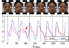
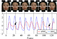
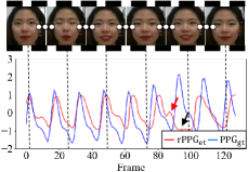
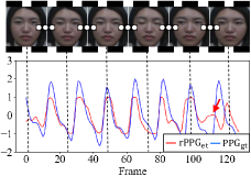
We first discuss the effect of makeup on the model performance. Among five datasets, MMVS contains subjects with makeup. Therefore, we split the MMVS into two subsets: MMVS-w/ makeup and MMVS-w/o makeup. Each subset contains a training set and a test set, which are respectively leveraged for model training and evaluation. HR estimation results are shown in Table XI. It can be seen that the results on MMVS-w/o makeup are better than those on MMVS-w/ makeup: e.g. the MAE is 2.90 on the former and 3.25 on the latter. Also, compared to the state of the art [20], which reflects a difference of 0.51 MAE between the two subsets, the influence of makeup on our method is smaller (i.e. 0.35 MAE difference between the two subsets). Fig. 11 further shows four estimated rPPG signals and their corresponding ground truth signals from subjects with makeup. We can see that some signal peaks are not well reconstructed (black arrows) while some are mistakenly reconstructed (red arrows). Makeup can cover the periodic color changes on faces, making it difficult to capture physiological clues for accurate rPPG estimation.
| Method | BP4D-Caucasian | BP4D-African | BP4D-Asian | ||||||
|---|---|---|---|---|---|---|---|---|---|
| MAE | RMSE | MAE | RMSE | MAE | RMSE | ||||
| Gideon et al. [20] | 3.68 | 4.96 | 0.88 | 5.15 | 7.00 | 0.82 | 3.22 | 4.40 | 0.92 |
| Ours | 2.89 | 4.13 | 0.93 | 4.69 | 6.21 | 0.85 | 2.54 | 3.72 | 0.96 |
 |
 |
| (a) Asian | (b) Caucasian |
 |
 |
| (c) African | (d) African |
6.2 Impact of ethnicity
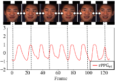
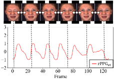
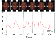
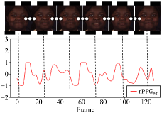
Next, we evaluate the model performance on subjects of different ethnicities. Among the five datasets, BP4D+ includes a wide coverage of ethnicities from Caucasian, African and Asian (East-Asian and Middle-East-Asian). We split the BP4D+ dataset into three subsets according to the subject ethnicities, i.e. BP4D-Caucasian, BP4D-African and BP4D-Asian. Each subset is divided into the training set and the test set. We train our method on the training set of each subset and evaluate it on the corresponding test set. HR estimation results on three test sets are shown in Table XII. Fig. 12 shows four concrete examples. From Table XII we can observe that both our approach and [20] perform the best on BP4D-Asian, the second best on BP4D-Caucasian and the worst on BP4D-African. Fig. 12(a) shows satisfactory signal periodicity on an Asian subject, while the estimated signals from African subjects in Fig. 12(c) and Fig. 12(d) are of low quality, especially their interbeat intervals vary significantly; we cannot observe the periodicity or quasi-periodicity from their waveforms. Note that BP4D+ does not include ground truth PPG signals but only the ground truth of HR.
According to [11], most RGB cameras are optimized to capture light skin tones more effectively than dark skin tones. Typically, a camera’s sensitivity is the greatest in the middle of the (0, 255) pixel range. That means dark skin tones of African subjects are likely to saturate the pixels, which would cause the skin color change by the physiological signal variation to be suppressed. Both our approach and [20] cannot obtain sufficient physiological clues for generating periodic rPPG signals on African subjects. Our finding is consistent with that reported in [11].
Given that BP4D+ is an ethnicity-imbalanced dataset (see Sec. 4.1), we further randomly sample 15 subjects of each ethnicity to construct the subsets BP4D-Caucasian, BP4D-Asian and BP4D-African again with balanced distribution. We train and test the three ethnicity-specific models on the three subsets respectively. According to our experiments on the HR estimation, the performance on BP4D-Caucasian and BP4D-Asian is still better than that on BP4D-African. For example, the MAE on BP4D-Caucasian and BP4D-Asian is 3.13 and 2.81, respectively; while on BP4D-African is 4.69. These results further validate our argument: the saturation of skin pixels of African subjects can suppress the pulsation-induced skin color change.
7 Conclusion
In this paper, we propose a new frequency-inspired self-supervised framework for facial video-based remote physiological measurement. Our approach consists of three key stages: data augmentation, signal extraction and network optimization. For data augmentation, we randomly select a video clip from a given facial video as the main input. We introduce the LFA module to generate sufficient negative samples from it. These negative samples contain rPPG signals with different frequencies to the input. Meanwhile, we also apply spatial augmentation on the input to obtain positive samples that share the same rPPG signal frequency to that of the input. For signal extraction, we design the REA module to extract complementary physiological clues from different face regions and aggregate them for an accurate rPPG estimation. In the REA module, a region-attention block is devised to focus the estimation on pulsation-sensitive skins and a spatio-temporal gating net is devised to combine temporal signals over different spatial regions. Last, for the network optimization, we propose a series of frequency-inspired losses to optimize estimated rPPG signals from the input’s augmentations and neighbors. Experiments on five datasets show the effectiveness and superiority of our method over state of the art.
Acknowledgments
This work was supported by the National Natural Science Foundation of China [No. 72293581, 72293580, 72188101 and 62103122], and the Fundamental Research Funds for the Central Universities.
References
- [1] X. Niu, S. Shan, H. Han, and X. Chen, “RhythmNet: End-to-End Heart Rate Estimation From Face via Spatial-Temporal Representation,” IEEE Transactions on Image Processing, vol. 29, pp. 2409–2423, 2020.
- [2] Z. Yue, S. Ding, S. Yang, H. Yang, Z. Li, Y. Zhang, and Y. Li, “Deep Super-Resolution Network for rPPG Information Recovery and Noncontact Heart Rate Estimation,” IEEE Transactions on Instrumentation and Measurement, vol. 70, pp. 1–11, 2021.
- [3] E. Lee, E. Chen, and C.-Y. Lee, “Meta-rPPG: Remote Heart Rate Estimation Using a Transductive Meta-learner,” in ECCV, 2020.
- [4] H. Lu, H. Han, and S. K. Zhou, “Dual-GAN: Joint BVP and Noise Modeling for Remote Physiological Measurement,” in CVPR, 2021.
- [5] X. Chen, J. Cheng, R. Song, Y. Liu, R. Ward, and Z. J. Wang, “Video-Based Heart Rate Measurement: Recent Advances and Future Prospects,” IEEE Transactions on Instrumentation and Measurement, vol. 68, no. 10, pp. 3600–3615, 2019.
- [6] B. P. Yan, W. H. S. Lai, C. K. Y. Chan, A. C. K. Au, B. Freedman, Y. C. Poh, and M.-Z. Poh, “High-Throughput, Contact-Free Detection of Atrial Fibrillation From Video With Deep Learning,” JAMA Cardiology, vol. 5, no. 1, p. 105, 2020.
- [7] X. Liu, X. Yang, D. Wang, A. Wong, L. Ma, and L. Li, “VidAF: A Motion-Robust Model for Atrial Fibrillation Screening From Facial Videos,” IEEE Journal of Biomedical and Health Informatics, vol. 26, no. 4, pp. 1672–1683, 2022.
- [8] E. M. Nowara, T. K. Marks, H. Mansour, and A. Veeraraghavan, “SparsePPG: Towards Driver Monitoring Using Camera-Based Vital Signs Estimation in Near-Infrared,” in CVPR Workshops, 2018.
- [9] W. Wang, A. C. den Brinker, S. Stuijk, and G. de Haan, “Algorithmic Principles of Remote PPG,” IEEE Transactions on Biomedical Engineering, vol. 64, no. 7, pp. 1479–1491, 2017.
- [10] Z. Yue, S. Ding, S. Yang, L. Wang, and Y. Li, “Multimodal Information Fusion Approach for Noncontact Heart Rate Estimation Using Facial Videos and Graph Convolutional Network,” IEEE Transactions on Instrumentation and Measurement, vol. 71, pp. 1–13, 2022.
- [11] D. McDuff, “Camera Measurement of Physiological Vital Signs,” ACM Computing Surveys, vol. 55, no. 9, pp. 1–40, 2023.
- [12] M.-Z. Poh, D. J. McDuff, and R. W. Picard, “Advancements in Noncontact, Multiparameter Physiological Measurements Using a Webcam,” IEEE Transactions on Biomedical Engineering, vol. 58, no. 1, pp. 7–11, 2011.
- [13] M.-Z. Poh and D. J. McDuff, “Non-contact, automated cardiac pulse measurements using video imaging and blind source separation,” Optics Express, vol. 18, no. 10, p. 10762, 2010.
- [14] G. de Haan and V. Jeanne, “Robust Pulse Rate From Chrominance-Based rPPG,” IEEE Transactions on Biomedical Engineering, vol. 60, no. 10, pp. 2878–2886, 2013.
- [15] R. Song, H. Chen, J. Cheng, C. Li, Y. Liu, and X. Chen, “PulseGAN: Learning to Generate Realistic Pulse Waveforms in Remote Photoplethysmography,” IEEE Journal of Biomedical and Health Informatics, vol. 25, no. 5, pp. 1373–1384, 2021.
- [16] X. Niu, Z. Yu, H. Han, X. Li, S. Shan, and G. Zhao, “Video-Based Remote Physiological Measurement via Cross-Verified Feature Disentangling,” in ECCV, 2020.
- [17] K. He, X. Zhang, S. Ren, and J. Sun, “Deep Residual Learning for Image Recognition,” in CVPR, 2016.
- [18] Z. Yu, W. Peng, X. Li, X. Hong, and G. Zhao, “Remote Heart Rate Measurement From Highly Compressed Facial Videos: An End-to-End Deep Learning Solution With Video Enhancement,” in ICCV, 2019.
- [19] Z. Yu, Y. Shen, J. Shi, H. Zhao, P. H. S. Torr, and G. Zhao, “PhysFormer: Facial Video-Based Physiological Measurement With Temporal Difference Transformer,” in CVPR, 2022.
- [20] J. Gideon and S. Stent, “The Way to my Heart is through Contrastive Learning: Remote Photoplethysmography from Unlabelled Video,” in ICCV, 2021.
- [21] S. Bobbia, R. Macwan, Y. Benezeth, A. Mansouri, and J. Dubois, “Unsupervised skin tissue segmentation for remote photoplethysmography,” Pattern Recognition Letters, vol. 124, pp. 82–90, 2019.
- [22] R. Stricker, S. Muller, and H.-M. Gross, “Non-contact video-based pulse rate measurement on a mobile service robot,” in IEEE International Symposium on Robot and Human Interactive Communication, 2014.
- [23] S. Koelstra, C. Muhl, M. Soleymani, Jong-Seok Lee, A. Yazdani, T. Ebrahimi, T. Pun, A. Nijholt, and I. Patras, “DEAP: A Database for Emotion Analysis Using Physiological Signals,” IEEE Transactions on Affective Computing, vol. 3, no. 1, pp. 18–31, 2012.
- [24] Z. Zhang, J. M. Girard, Y. Wu, X. Zhang, P. Liu, U. Ciftci, S. Canavan, M. Reale, A. Horowitz, H. Yang, J. F. Cohn, Q. Ji, and L. Yin, “Multimodal Spontaneous Emotion Corpus for Human Behavior Analysis,” in CVPR, 2016.
- [25] R. Macwan, Y. Benezeth, and A. Mansouri, “Heart rate estimation using remote photoplethysmography with multi-objective optimization,” Biomedical Signal Processing and Control, vol. 49, pp. 24–33, 2019.
- [26] D. J. McDuff, E. B. Blackford, and J. R. Estepp, “Fusing Partial Camera Signals for Noncontact Pulse Rate Variability Measurement,” IEEE Transactions on Biomedical Engineering, vol. 65, no. 8, pp. 1725–1739, 2018.
- [27] M. Hu, F. Qian, D. Guo, X. Wang, L. He, and F. Ren, “ETA-rPPGNet: Effective Time-Domain Attention Network for Remote Heart Rate Measurement,” IEEE Transactions on Instrumentation and Measurement, vol. 70, pp. 1–12, 2021.
- [28] M. Noroozi and P. Favaro, “Unsupervised Learning of Visual Representations by Solving Jigsaw Puzzles,” in ECCV, 2016.
- [29] S. Gidaris, P. Singh, and N. Komodakis, “Unsupervised Representation Learning by Predicting Image Rotations,” in ICLR, 2018.
- [30] M. Noroozi, H. Pirsiavash, and P. Favaro, “Representation Learning by Learning to Count,” in ICCV, 2017.
- [31] C. Vondrick, H. Pirsiavash, and A. Torralba, “Anticipating Visual Representations from Unlabeled Video,” in CVPR, 2016.
- [32] X. Wang and A. Gupta, “Unsupervised Learning of Visual Representations Using Videos,” in ICCV, 2015.
- [33] T. Chen, S. Kornblith, M. Norouzi, and G. Hinton, “A Simple Framework for Contrastive Learning of Visual Representations,” in ICML, 2020.
- [34] K. He, H. Fan, Y. Wu, S. Xie, and R. Girshick, “Momentum Contrast for Unsupervised Visual Representation Learning,” in CVPR, 2020.
- [35] T. Pan, Y. Song, T. Yang, W. Jiang, and W. Liu, “VideoMoCo: Contrastive Video Representation Learning with Temporally Adversarial Examples,” in CVPR, 2021.
- [36] X. Chen and K. He, “Exploring Simple Siamese Representation Learning,” in CVPR, 2021.
- [37] X. Wang and G.-J. Qi, “Contrastive Learning with Stronger Augmentations,” IEEE Transactions on Pattern Analysis and Machine Intelligence, pp. 1–12, 2022.
- [38] R. Qian, T. Meng, B. Gong, M.-H. Yang, H. Wang, S. Belongie, and Y. Cui, “Spatiotemporal Contrastive Video Representation Learning,” in CVPR, 2021.
- [39] A. Spurr, A. Dahiya, X. Wang, X. Zhang, and O. Hilliges, “Self-Supervised 3D Hand Pose Estimation from monocular RGB via Contrastive Learning,” in ICCV, 2021.
- [40] Y. Wang, Y. Jiang, J. Li, B. Ni, W. Dai, C. Li, H. Xiong, and T. Li, “Contrastive Regression for Domain Adaptation on Gaze Estimation,” in CVPR, 2022.
- [41] R. Dangovski, L. Jing, C. Loh, S. Han, A. Srivastava, B. Cheung, P. Agrawal, and M. Soljačić, “Equivariant Contrastive Learning,” in ICLR, 2022.
- [42] S. Tukra and S. Giannarou, “Stereo Depth Estimation via Self-supervised Contrastive Representation Learning,” in MICCAI, 2022.
- [43] R. A. Jacobs, M. I. Jordan, S. J. Nowlan, and G. E. Hinton, “Adaptive Mixtures of Local Experts,” Neural Computation, vol. 3, no. 1, pp. 79–87, 1991.
- [44] A. Srivastava, R. Su, and A. Weigend, “Data mining for features using scale-sensitive gated experts,” IEEE Transactions on Pattern Analysis and Machine Intelligence, vol. 21, no. 12, pp. 1268–1279, 1999.
- [45] S. Masoudnia and R. Ebrahimpour, “Mixture of experts: A literature survey,” Artificial Intelligence Review, vol. 42, 2014.
- [46] J. V. Hansen, “Combining predictors: comparison of five meta machine learning methods,” Information Sciences, vol. 119, no. 1, pp. 91–105, 1999.
- [47] S. E. Yuksel, J. N. Wilson, and P. D. Gader, “Twenty Years of Mixture of Experts,” IEEE Transactions on Neural Networks and Learning Systems, vol. 23, no. 8, pp. 1177–1193, 2012.
- [48] A. Subasi, “EEG signal classification using wavelet feature extraction and a mixture of expert model,” Expert Systems with Applications, vol. 32, no. 4, pp. 1084–1093, 2007.
- [49] M. Emad, M. Peemen, and H. Corporaal, “MoESR: Blind Super-Resolution using Kernel-Aware Mixture of Experts,” in WACV, 2022.
- [50] Y. Shi, B. Paige, P. Torr et al., “Variational mixture-of-experts autoencoders for multi-modal deep generative models,” in NIPS, 2019.
- [51] J. Ma, Z. Zhao, X. Yi, J. Chen, L. Hong, and E. H. Chi, “Modeling Task Relationships in Multi-task Learning with Multi-gate Mixture-of-Experts,” in ACM SIGKDD, 2018.
- [52] M. Sahasrabudhe, P. Sujobert, E. I. Zacharaki, E. Maurin, B. Grange, L. Jallades, N. Paragios, and M. Vakalopoulou, “Deep Multi-Instance Learning Using Multi-Modal Data for Diagnosis of Lymphocytosis,” IEEE Journal of Biomedical and Health Informatics, vol. 25, no. 6, pp. 2125–2136, 2021.
- [53] J. Li, Z. Yu, and J. Shi, “Learning Motion-Robust Remote Photoplethysmography through Arbitrary Resolution Videos,” in AAAI, 2023.
- [54] Z. Yu, Y. Shen, J. Shi, H. Zhao, Y. Cui, J. Zhang, P. Torr, and G. Zhao, “PhysFormer++: Facial Video-Based Physiological Measurement with SlowFast Temporal Difference Transformer,” International Journal of Computer Vision, vol. 131, pp. 1307–1330, 2023.
- [55] K. Zhang, Z. Zhang, Z. Li, and Y. Qiao, “Joint Face Detection and Alignment Using Multitask Cascaded Convolutional Networks,” IEEE Signal Processing Letters, vol. 23, no. 10, pp. 1499–1503, 2016.
- [56] Z. Yu, X. Li, and G. Zhao, “Facial-Video-Based Physiological Signal Measurement: Recent advances and affective applications,” IEEE Signal Processing Magazine, vol. 38, no. 6, pp. 50–58, 2021.
- [57] R. Szeto, X. Sun, K. Lu, and J. J. Corso, “A Temporally-Aware Interpolation Network for Video Frame Inpainting,” IEEE Transactions on Pattern Analysis and Machine Intelligence, vol. 42, no. 5, pp. 1053–1068, 2020.
- [58] Y. Li, P. Jin, F. Yang, C. Liu, M.-H. Yang, and P. Milanfar, “COMISR: Compression-Informed Video Super-Resolution,” in ICCV, 2021.
- [59] J. Hu, L. Shen, S. Albanie, G. Sun, and E. Wu, “Squeeze-and-Excitation Networks,” IEEE Transactions on Pattern Analysis and Machine Intelligence, vol. 42, no. 8, pp. 2011–2023, 2020.
- [60] A. v. d. Oord, Y. Li, and O. Vinyals, “Representation Learning with Contrastive Predictive Coding,” arXiv:1807.03748, 2019.
- [61] S. Kim, S. Jeong, E. Kim, I. Kang, and N. Kwak, “Self-supervised Pre-training and Contrastive Representation Learning for Multiple-choice Video QA,” in AAAI, 2021.
- [62] A. Diba, V. Sharma, R. Safdari, D. Lotfi, M. S. Sarfraz, R. Stiefelhagen, and L. Van Gool, “Vi2CLR: Video and Image for Visual Contrastive Learning of Representation,” in ICCV, 2021.
- [63] R. Song, S. Zhang, C. Li, Y. Zhang, J. Cheng, and X. Chen, “Heart Rate Estimation From Facial Videos Using a Spatiotemporal Representation With Convolutional Neural Networks,” IEEE Transactions on Instrumentation and Measurement, vol. 69, no. 10, pp. 7411–7421, Oct. 2020.
- [64] D. P. Kingma and J. Ba, “Adam: A Method for Stochastic Optimization,” in ICLR, 2017.
- [65] P. Van Gent, H. Farah, N. Van Nes, and B. Van Arem, “Analysing Noisy Driver Physiology Real-Time Using Off-the-Shelf Sensors: Heart Rate Analysis Software from the Taking the Fast Lane Project,” Journal of Open Research Software, vol. 7, no. 1, p. 32, 2019.
- [66] W. Verkruysse, L. O. Svaasand, and J. S. Nelson, “Remote plethysmographic imaging using ambient light,” Optics Express, vol. 16, no. 26, p. 21434, 2008.
- [67] X. Niu, H. Han, S. Shan, and X. Chen, “SynRhythm: Learning a Deep Heart Rate Estimator from General to Specific,” in ICPR, 2018.
- [68] J. Park, K. Ko, C. Lee, and C.-S. Kim, “BMBC: Bilateral Motion Estimation with Bilateral Cost Volume for Video Interpolation,” in ECCV, 2020.
- [69] J. Park, C. Lee, and C.-S. Kim, “Asymmetric Bilateral Motion Estimation for Video Frame Interpolation,” in ICCV, 2021.
- [70] S. Mendez-Diaz, J. C. Serrano-García, R. Zenit, and J. A. Hernández-Cordero, “Power spectral distributions of pseudo-turbulent bubbly flows,” Physics of Fluids, vol. 25, no. 4, p. 043303, 2013.
- [71] F. Wang and H. Liu, “Understanding the Behaviour of Contrastive Loss,” in CVPR, 2021.
![[Uncaptioned image]](/html/2210.15401/assets/figs/bio-yzj.jpg) |
Zijie Yue received his B.E. and Ph.D. degrees from Hefei University of Technology in 2017 and 2023, respectively. He is currently a postdoctoral researcher at Tongji University. His current research is in the area of remote physiological measurement, computer vision, and machine learning. |
![[Uncaptioned image]](/html/2210.15401/assets/figs/bio-miaojing.jpg) |
Miaojing Shi (Senior Member, IEEE) received the Ph.D. degree from Peking University in 2015. He also engaged with a joint Ph.D. program with the University of Oxford and INRIA Rennes for a year. He held a postdoctoral position at the University of Edinburgh and was a Research Scientist at INRIA Rennes. Between 2020 and 2022, he has been a Lecturer with the Department of Informatics, King’s College London. Since 2023, he becomes a Full Professor at Tongji University and a visiting Senior Lecturer at King’s. He has authored or coauthored over 50 publications. His current research focus is on visual learning and understanding, with multi-task and limited supervision. |
![[Uncaptioned image]](/html/2210.15401/assets/x26.png) |
Shuai Ding received his Ph.D. degree in management science and engineering from Hefei University of Technology, Hefei, China, in 2011. He has been a Visiting Scholar with the University of Pittsburgh, Pittsburgh, PA, USA. He is currently a Professor with the School of Management, Hefei University of Technology. His research interests include smart healthcare, medical artificial intelligence, and management information systems. |