EmulART: Emulating Radiative Transfer - A pilot study on autoencoder based dimensionality reduction for radiative transfer models
(accepted in Neural Computing and Applications)

Abstract

Dust is a major component of the interstellar medium. Through scattering, absorption and thermal re-emission, it can profoundly alter astrophysical observations. Models for dust composition and distribution are necessary to better understand and curb their impact on observations. A new approach for serial and computationally inexpensive production of such models is here presented.

Traditionally these models are studied with the help of radiative transfer modelling, a critical tool to understand the impact of dust attenuation and reddening on the observed properties of galaxies and active galactic nuclei. Such simulations present, however, an approximately linear computational cost increase with the desired information resolution.

Our new efficient model generator proposes a denoising variational autoencoder (or alternatively PCA), for spectral compression, combined with an approximate Bayesian method for spatial inference, to emulate high information radiative transfer models from low information models.

For a simple spherical dust shell model with anisotropic illumination, our proposed approach successfully emulates the reference simulation starting from less than 1% of the information. Our emulations of the model at different viewing angles present median residuals below 15% across the spectral dimension, and below 48% across spatial and spectral dimensions. EmulART infers estimates for $\sim$85% of information missing from the input, all within a total running time of around 20 minutes, estimated to be 6$\times$ faster than the present target high information resolution simulations, and up to 50$\times$ faster when applied to more complicated simulations.

1 Introduction

Cosmic dust is ubiquitous in the Universe, particularly present in the interstellar medium (ISM) (Zhukovska et al, 2008) and in the line of sight towards astrophysical objects such as supernovae remnants (Rho et al, 2009), galaxies (Dunne et al, 2011) and active galactic nuclei (AGN) (AGN, Haas et al, 2000). Dust grains absorb and scatter UV/optical radiation and re-emit that energy at infrared wavelengths, and are thus responsible for both attenuation and reddening of light in the line of sight, which also impact distance measurements for cosmology when using “standard candles” such as supernovae (Betoule et al, 2014). Moreover, scattering on the dust grains and dichroic absorption in the dusty medium may lead to polarization of the light as it traverses the interstellar medium.

The effect these processes - of dust absorption, scattering and emission - have on the light detected from astronomical objects must be accounted when studying their intrinsic properties. Moreover, the nature of the dust can also inform us on physical and chemical processes related to its own history, from formation, variation in composition, growth and destruction in different astrophysical structures such as accretion disks, clouds and galaxies, as well as its interaction with magnetic fields through dust grain alignment. The analysis of the aforementioned interactions requires performing radiative transfer (RT) calculations (Steinacker et al, 2013), allowing us to simulate the light path, from the source to the observer, depending on the physical properties of the emitting source embedded in dust structures of different geometries, sizes and composition. Comparing various RT models, based on different simulated properties, to global and pixel-by-pixel spectral energy distributions (SEDs) obtained in astronomical observations we can infer valuable information on the properties of the light sources, as well as the distribution and properties of the dust (André et al, 2010; Cox et al, 2012; Fritz et al, 2012).

Observations of molecular clouds(Beech, 1987; Falgarone et al, 1991) have shown that dust distributions are often inhomogeneous and complex, consequently the understanding of their intrinsic properties requires 3D radiative transfer calculations. This type of non-local and non-linear problem requires calculations which are computationally very costly (Steinacker et al, 2013), this has prompted the search for alternative non-analytic approximate ways to address them. One of the most successful ways is Monte Carlo Radiative Transfer (MCRT, Mattila, 1970; Roark et al, 1974).

Monte Carlo Radiative Transfer methods simulate a large number of test photons, that propagate from their emission by a source through their journeys through the dusty medium. At every stage the characteristics that define their paths are determined by generating numbers from the probability density function most suited for each process they may undergo (absorption, scattering, re-emission, etc). At the end of the simulation, the radiation field is recovered from a statistical analysis of the photon paths. As an ensemble, the distribution of particles provides a good representation of the radiative transfer, as long as a sufficient number of photons is chosen.

Stellar Kinematics Including Radiative Transfer (SKIRT, Baes et al, 2011; Camps and Baes, 2015) is an MCRT suite that offers some built-in source templates, geometries, dust characterizations, spatial grids, and instruments, as well as an interface so that a user can easily describe a physical model. The user can in this way avoid coding the physics that describes both the source (e.g. AGN or galaxy type, observation perspective, emission spectrum) and environment (between the simulated source and observer, such as dust grain type and orientation, dust density distribution, etc) but instead design a model of modular complexity by following a Q&A prompt (itself adaptable to the user expertise).

MCRT simulations suffer from computational limitations, namely the memory requirement scaling with the volume grid density, and the processing time scaling quasi-linearly with the amount of photons simulated (Camps and Baes, 2020). Autoencoders (Zhuang et al, 2021) together with collocation strategies (Guo et al, 2019) have been applied to solve complex interactions such as the ones described above, our approach differs by attempting to upscale the information density within a simulated data product instead. Considering that the objects and phenomena modeled by MCRT simulations present non-random spatial structures with heavily correlated spectral features, we tackle the computational cost issue through the development of an emulator that can achieve HPN-like MCRT models by exploring and implementing an autoencoder neural network in combination with Integrated Nested Laplace Approximation (INLA, Rue et al, 2009), an approximate method for Bayesian inference of spatial maps modeled with Gaussian Markov random fields, on LPN-like MCRT simulations. The results are then compared against an analogous implementation employing principal component analysis (PCA).

Section 2 provides a brief highlight of the employed methods. Section 3 describes our pipeline architecture and some of steps that lead to its development. Results and performance evaluation follow in Section 4. Section 5 presents our perspective on the significance of the obtained results and provides the steps to follow in order to both improve and generalize them in future developments.

All files concerning this work (SKIRT simulations, R scripts, neural network models, emulation products and performance statistics) can be obtained from our repository.

2 Methods

To reduce the computational cost of SKIRT simulations, without compromising, as much as possible, the quality of the resulting models, an autoencoder, i.e. a dimensionality reduction neural network, is implemented to compress the spectral information within LPN spectroscopic data cubes. Then approximate Bayesian inference is performed with INLA on the spatial information of the compressed feature maps. Lastly, the reconstructed feature maps are decompressed to an HPN emulation.

2.1 SKIRT

As previously state, SKIRT allows the creation of models by prompting a Q&A. Through it the user can configure any one- to three-dimensional geometry and combine multiple sources and media components, each with their own spatial distribution and physical properties, by either employing the built-in library or importing components from hydrodynamic simulations. Media types include dust, electrons and neutral hydrogen; the user can configure their own mixture, including optical properties and size distributions or simply choose from the available built-in mixtures. The included instruments allow the ”observation” and recording of spectra, broad-band images or spectroscopic data cubes.

SKIRT uses Monte Carlo method for tracing photon packets through the spatial domain (both regular and adaptive spatial grids area available, as well as some optimized for 1D or 2D models), these packets are wavelength sampled from the source/medium spectrum (the wavelength grids can be separately configured for both storing the radiation field and for discretizing medium emission spectra). As they progress through the spatial grid cells, these photon packets can experience different physical interactions, such as multiple anisotropic scattering, absorption and (re-)emission by the transfer medium, Doppler shifts due to kinematics of sources and/or media, polarization caused by scattering off dust grains as well as polarized emission, among others.

The present application is intended for the combination of both spatial and spectral information. The outputs used here will be spectroscopic data cubes, these are in the flexible image transport system (FITS) format (Wells et al, 1981) and are composed of 2D spatial distributions at the desired wavelength bins.

The simulated spatial flux densities vary according to the amount of photons/photon packets simulated. The simulation starts by assigning some energy to those photons following the spectral energy distribution (SED) of a given astrophysical source, ensuring that no matter how many photons are simulated the spectral information is preserved. Simulations with a lower photon number (LPN) will consequently display fewer spatial positions with information (non-zero flux) and some of these pixels will have higher flux, some lower, i.e. the SED will have lower signal to noise ratio than in simulations with higher photon number (HPN). SKIRT has already been employed in the study of various galaxies (De Looze et al, 2014; Viaene et al, 2017; Verstocken et al, 2020), AGN (Stalevski et al, 2016, 2019) and other objects.

2.2 Dimensionality Reduction

Dimensionality reduction methods can more familiarly be called as compressors. These are methods that analyse and transform data from a high-dimensional space into a low-dimensional space while attempting to retain as much meaningful properties of the original data as possible. Working in high-dimensional spaces can be undesirable for many reasons; raw data are often sparse as a consequence of the curse of dimensionality, and analyzing the data usually becomes computationally intractable. Popular dimensionality reduction techniques in astronomy include PCA (Krone-Martins and Moitinho, 2014; Logan and Fotopoulou, 2020) and Non-Negative Matrix Factorization (NMF, Ren et al, 2018; Boulais et al, 2021).

Autoencoder networks are an alternative method which has been gaining attention within the astronomy, astrophysics and cosmology community (Ichinohe and Yamada, 2019; Ralph et al, 2019; O’Briain et al, 2020; Portillo et al, 2020; Jia et al, 2020; Wang et al, 2021).

2.2.1 Denoising Variational Autoencoders

Autoencoders (AEs) are a type of neural network architecture employed to learn compressed representations of data. In such architectures the input and output layers are equal, and the hidden layers display a funneling in and out scheme in regards to the number of neurons per layer, with the middle layer having the least amount of neurons and the input and output layers having the most. The models built this way can be seen as the coupling of a compressor/encoder and a decompressor/decoder, the first generating a more (ideally) fundamental representation of the data, and the second bringing it back to its initial feature space. After training, the encoder can be coupled at the beginning of other architectures, providing them with more efficient features from which to learn from. Interesting to note that AEs have shown promise as auxiliary tools in citizen science projects, such as the Radio Galaxy Zoo (Ralph et al, 2019).

Alternative ways of training this kind of network exist, such as:

• Having multiple instances of each data point, resulting from the injection of noise or from a set of transformations. Each instance of the same data point is then matched to the same output with the aim of making the model robust to noise and/or invariant to those transformations.

• Having the mid layer composed by two complementary layers of neurons (a mean layer and a standard deviation layer) instead of a single layer. Complemented with an appropriate loss function, the model will learn approximate distributions of values instead of single values, making it more robust and allowing for the decoder to also become a generator of different, yet statistically identical, examples.

Such strategies fall under different categories such as denoising autoencoders (DAEs) (Kopf et al, 2021) and variational autoencoders (VAEs) (Hinton and Salakhutdinov, 2006) respectively. In this work we implement both, a denoising variational autoencoder (DVAE).

(Jiwoong Im et al, 2015) showed that the DVAE, by introducing a corruption model, can lead to an encoder that covers a broader class of distributions when compared to a regular VAE (the corruption model may however remove the information necessary for reconstruction). In this context the loss function, $\mathcal{L}_{DVAE}$, to be minimized is given by the weighted sum of the Kullback-Leibler divergence (which influences the encoder) and the reconstruction error (see Eq. 1), similarly to a VAE, with the difference that the encoder now learns to approximate a prior $p(z)$ given corrupted examples and that in this case the reconstruction error can be interpreted as a denoising criterion:

$$\mathcal{L}_{DVAE}\propto a_{1}\mathbb{KL}(q(z\mid y^{\prime})\mid p(z))+a_{2}\ln{p(y\mid z)}\,\,,$$ (1)

where $\mathbb{KL}$ refers to the Kullback-Liebler divergence, $y^{\prime}\sim q(y^{\prime}\mid y)$ is a sample of the corruption model, $p(z)$ is the prior for the latent feature, $q(z\mid y^{\prime})$ models the encoder, $p(y\mid z)$ models the decoder/generator and ($a_{1}$, $a_{2}$) are weights. For more details the reader is referred to (Jiwoong Im et al, 2015; Doersch, 2016).

2.2.2 Principal Component Analysis

Principal Component Analysis (PCA) is a method that analyzes the feature space of the training data and creates orthogonal vectors (linear combinations of the initial variables) whose direction indicates the most variability. These new vectors in the transformed data set are called eigenvectors, or principal components, while the eigenvalues represent the coefficients attached to eigenvectors and give the relative amount of variance carried by each principal component.

PCA transforms the original space through rotation of its axes and re-scaling of the axes range. The first new PC is aligned with the direction of largest variance in the data. The second PC should also maximize the variance, while being orthogonal to the first, and respectively for the remaining PCs. Mathematically, these directions can be determined through the covariance matrix, as expressed in Eq. 2:

$$\Sigma_{ff^{\prime}}=\sum_{j=1}^{j=N}\frac{(X_{f}^{j}-\bar{X}_{f})(X_{f^{\prime}}^{j}-\bar{X}_{f^{\prime}})}{N}\,\,,$$ (2)

where $X_{f}$ is the mean of all values at feature $f$ and $N$ is the total number of data points (for more details and a modern review on PCA we suggest (Jolliffe and Cadima, 2016)). Once $\Sigma_{ff^{\prime}}$ is diagonalized, the PCs are its eigenvectors, the first PC being the one with the largest associated eigenvalue and so on.

PCs are uncorrelated and frequently the information is compressed into the first $K$ components, with $K\ll M$ (where $M$ is the total number of features of the original space).

A data point from the original data set can then be reasonably recovered using those $K$ PCs,

$$\hat{\bfX}\approx\bar{\bfX}+\sum_{m=1}^{m=K}c_{m}\bfP_{m}\,\,,$$ (3)

where $\bf\bar{X}$ represents the mean of all data points, $\bfP_{m}$ is the m-th PC and $c_{m}$ is the projection of the data point on $\bfP_{m}$.

Using all the $M$ PCs the reconstruction becomes identical to the original data, but with a new basis that captures a large fraction of the variance in a small number of components $K$, dimensionality reduction is achieved. In this work we used two approaches to determine $K$ (see Section 3.4).

Further discussion on the importance of PCA and its applications in astronomy can be found in e.g. (Ishida and de Souza, 2011; Ishida et al, 2011; Sasdelli et al, 2014).

2.3 Spatial Approximate Bayesian Inference

Bayesian inference (BI) refers to a family of methods of statistical inference where a hypothetical probabilistic model is updated, following Bayes theorem (Eq. 4), whenever new data is obtained. Bayes theorem allows to calculate a posterior distribution $p(\theta\mid y)$ (the conditional probability of $\theta$ occurring given $y$) by weighting in $p(y\mid\theta)$ (the likelihood of $y$ occurring given $\theta$), $p(\theta)$ (estimation of the probability distribution of $\theta$ before observing $y$, also designated as a prior), and $p(y)$ (the marginal probability of $y$, obtained from integrating $\theta$ out of $p(y\mid\theta)$):

$$p(\theta\mid y)=\frac{p(y\mid\theta)}{p(y)}p(\theta)\,\,,$$ (4)

$$p(y)=\int{p(y\mid\theta)p(\theta)\textrm{d}\theta}\,\,.$$ (5)

This kind of update is of utmost relevance in the dynamical analysis of data streams or in the analysis of correlated data, and has been proposed in astronomy, from the study of variable stars (Zorich et al, 2020) to 3-D mapping of the Milky Way (Babusiaux et al, 2020).

Approximation techniques (Tierney and Kadane, 1986; Hinton and van Camp, 1993; Minka, 2013) have been developed over the years in order to help curb the very time-consuming process of sampling the whole likelihood $p(y\mid\theta)$. To this end, we here implement the Integrated Nested Laplace Approximation (INLA, Rue et al, 2009).

2.3.1 Integrated Nested Laplace Approximation

INLA is an approximate BI method that accounts for spatial correlations between observed data points to recover an assumed Gaussian latent field and, in doing so, it is not only capable of predicting unobserved points of that field but also of correcting noisy observed ones, as well as associating a variance to those inferences.

Most techniques for calculating posterior distribution rely on Markov chain Monte Carlo (MCMC, Collins et al, 1974) methods. In this class of sampling-based numerical methods, the posterior distribution is obtained after many iterations, which is often computationally expensive. INLA provides a novel approach for faster BI. While MCMC methods draw a sample from the joint posterior distribution, the Laplace approximation is a method that approximates posterior distributions of the model parameters to Gaussians, which is computationally more effective. Within the INLA framework, the posterior distribution of the latent Gaussian variables $\boldsymbol{x}$ and hyper-parameters of the model $\boldsymbol{\theta}$ is:

$$p(\boldsymbol{x},\boldsymbol{\theta}\mid\boldsymbol{y})=\frac{p(\boldsymbol{y}\mid\boldsymbol{x},\boldsymbol{\theta})~{}p(\boldsymbol{x},\boldsymbol{\theta})}{p(\boldsymbol{y})}\propto p(\boldsymbol{y}\mid\boldsymbol{x},\boldsymbol{\theta})~{}p(\boldsymbol{x},\boldsymbol{\theta}),$$ (6)

where $\boldsymbol{y}=(y_{1},...,y_{n})$ represents a set of observations. Each observation is treated with a latent Gaussian effect, with each $x_{i}$ (a Gaussian distribution of mean value $\mu_{i}$ and standard deviation $\sigma_{i}$) corresponding to an observation $y_{i}$, where $i\in[1,...,n]$. The observations are conditionally independent given the latent effect $\boldsymbol{x}$ and the hyper-parameters $\boldsymbol{\theta}$, the model likelihood is then:

$$p(\boldsymbol{y}\mid\boldsymbol{x},\boldsymbol{\theta})=\prod_{i}p(y_{i}\mid x_{i},\boldsymbol{\theta})\,\,.$$ (7)

The joint distribution of the latent effects and the hyper-parameters, $p(\boldsymbol{x},\boldsymbol{\theta})$ can be written as $p(\boldsymbol{x}\mid\boldsymbol{\theta})~{}p(\boldsymbol{\theta})$, where $p(\boldsymbol{\theta})$ represents the prior distribution of hyper-parameters $\boldsymbol{\theta}$. It is assumed that the spatial information can be treated as a discrete sampling of an underlying continuous spatial field, a latent Gaussian Markov Random Field (GMRF), that takes into account the spatial correlations, and whose hyper-parameters are inferred in the process. For a GMRF, the posterior distribution of the latent effects is:

$$p(\boldsymbol{x}\mid\boldsymbol{\theta})\propto\mid\boldsymbol{Q}(\boldsymbol{\theta})\mid^{1/2}\exp{-\frac{1}{2}\boldsymbol{x}^{T}\boldsymbol{Q}(\boldsymbol{\theta})~{}\boldsymbol{x}}\,\,,$$ (8)

where $\boldsymbol{Q}(\boldsymbol{\theta})$ represents a precision matrix, or inverse of a covariance matrix, which depends on a vector of hyper-parameters $\boldsymbol{\theta}$. This kernel matrix is what actually treats the spatial correlation between neighboring observations. Using equation 6, the joint posterior distribution of the latent effects and hyper-parameters can be written as:

$$\begin{aligned} p(\boldsymbol{x},\boldsymbol{\theta}\mid\boldsymbol{y})\propto p(\boldsymbol{\theta})\mid\boldsymbol{Q}(\boldsymbol{\theta})\mid^{1/2}\exp{-\frac{1}{2}\boldsymbol{x}^{T}\boldsymbol{Q}(\boldsymbol{\theta})~{}\boldsymbol{x}}\prod_{i}p(y_{i}\mid x_{i},\boldsymbol{\theta})=\\ =p(\boldsymbol{\theta})\mid\boldsymbol{Q}(\boldsymbol{\theta})\mid^{1/2}\exp{-\frac{1}{2}\boldsymbol{x}^{T}\boldsymbol{Q}(\boldsymbol{\theta})~{}\boldsymbol{x}+\sum_{i}\log(p(y_{i}\mid x_{i},\boldsymbol{\theta}))}\,\,.\end{aligned}$$ (9)

Instead of obtaining the exact posterior distribution from equation 9 INLA approximates the posterior marginals of the latent effects and hyper-parameters, its key methodological feature is to use appropriate approximations for the following integrals:

$$p(x_{i}\mid\boldsymbol{y})=\int p(x_{i}\mid\boldsymbol{\theta},\boldsymbol{y})p(\boldsymbol{\theta}\mid\boldsymbol{y})~{}d\boldsymbol{\theta}$$ (10)

$$p(\theta_{j}\mid\boldsymbol{y})=\int p(\boldsymbol{\theta}\mid\boldsymbol{y})~{}d\boldsymbol{\theta}_{-j},$$ (11)

where $\boldsymbol{\theta}_{-j}$ is a vector of hyper-parameters $\boldsymbol{\theta}$ without element $\theta_{j}$.

INLA constructs nested approximations:

$$\tilde{p}(x_{i}\mid\boldsymbol{y})=\int\tilde{p}(x_{i}\mid\boldsymbol{\theta},\boldsymbol{y})\tilde{p}(\boldsymbol{\theta}\mid\boldsymbol{y})~{}d\boldsymbol{\theta}\,\,,$$ (12)

$$\tilde{p}(\theta_{j}\mid\boldsymbol{y})=\int\tilde{p}(\boldsymbol{\theta}\mid\boldsymbol{y})~{}d\boldsymbol{\theta}_{-j}\,\,,$$ (13)

where $\tilde{p}(\cdot\mid\cdot)$ is an approximated posterior density. Using the Laplace approximation, the posterior marginals of hyper-parameters $p(\boldsymbol{\theta}\mid\boldsymbol{y})$ at a specific value $\boldsymbol{\theta}=\boldsymbol{\theta}_{j}$ can be written as:

$$\tilde{p}(\boldsymbol{\theta}_{j}\mid\boldsymbol{y})\propto\frac{p(\boldsymbol{x},\boldsymbol{\theta}_{j},\boldsymbol{y})}{\tilde{p}_{G}(\boldsymbol{x}\mid\boldsymbol{\theta}_{j},\boldsymbol{y})}\propto\frac{p(\boldsymbol{y}\mid\boldsymbol{x},\boldsymbol{\theta}_{j})p(\boldsymbol{x}\mid\boldsymbol{\theta}_{j})p(\boldsymbol{\theta}_{j})}{\tilde{p}_{G}(\boldsymbol{x}\mid\boldsymbol{\theta}_{j},\boldsymbol{y})}\mid_{\boldsymbol{x}=\boldsymbol{x}^{*}(\boldsymbol{\theta}_{j})}\,\,,$$ (14)

$$\tilde{p}_{G}(\boldsymbol{x}\mid\boldsymbol{\theta},\boldsymbol{y})\propto\exp{-\frac{1}{2}\boldsymbol{x}^{T}\boldsymbol{Q}(\boldsymbol{\theta})~{}\boldsymbol{x}+\sum_{i}g_{i}(x_{i})}\,\,,$$ (15)

where $\tilde{p}_{G}(\boldsymbol{x}\mid\boldsymbol{\theta},\boldsymbol{y})$ is the Gaussian approximation to the full conditional of $\boldsymbol{x}$, and $\boldsymbol{x^{*}}(\boldsymbol{\theta}_{j})$ is the mode of the full conditional $\boldsymbol{x}$ for given $\boldsymbol{\theta}_{j}$. The posterior marginals of the latent effects are then numerically integrated as follows:

$$\tilde{p}(x_{i}\mid\boldsymbol{y})\backsimeq\sum_{j}\tilde{p}(x_{i}\mid\boldsymbol{\theta}_{j},\boldsymbol{y})\tilde{p}(\boldsymbol{\theta}_{j}\mid\boldsymbol{y})\Delta_{j}\,\,,$$ (16)

where $\Delta_{j}$ represents the integration step.

A good approximation for $\tilde{p}(x_{i}\mid\boldsymbol{\theta},\boldsymbol{y})$ is required and INLA offers three different options: Gaussian approximation, Laplace approximation and simplified Laplace approximation (Rue et al, 2009). In this work we used the simplified Laplace approximation, which represents a compromise between the accuracy of the Laplace approximation and the reduced computational cost achieved with the Gaussian approximation.

INLA has been shown (Rue et al, 2009) to greatly outperform MCMC sampling under limited computational power/time conditions, with the estimation error of INLAs results being invariably smaller than those of MCMC. Other approximated inference methods exist, such as variational Bayes (Hinton and van Camp, 1993) and expectation-propagation (Minka, 2013), however these methods are not only slower, but they struggle with estimating the variance of the posterior since they execute iterative calculations instead of analytic approximations, unlike INLA (Rue et al, 2009).

INLA suffers nonetheless from some limitations. The first, already mentioned above, is that to get meaningful results the latent field to be inferred must be Gaussian - which is not always the case -, and it must display conditional independence properties; the second is that for fast inference it is required that the number of hyper-parameters (characterizers of the parameter models) should be inferior to 6, and that the number of available observations of the field to infer be much smaller than the size of that field.

INLA is freely available as an R package (Bachl et al, 2019), and it has already been shown to: 1) be capable of recovering structures in scalar and vector fields, with great fidelity, out of sparse sets of observations, and even of inferring structures never seen before; 2) be robust to noise injections (González-Gaitán et al, 2019). We refer to (Rue et al, 2009; Gómez-Rubio, 2021) for more details on the mathematical background of INLA and the methods it employs.

3 Implementation

This section describes both the dataset, the combination of a DVAE/PCA with INLA to enhance low information density SKIRT simulation data cubes and the tools to do so.

Our pilot pipeline aims to emulate radiative transfer models, as such we named it EmulART. All scripts were written and executed under R (R Core Team, 2021) (version 3.6.3) and make use of the Keras API (Allaire and Chollet, 2021).

The DVAE architecture was adapted from the one described in the Keras https://tensorflow.rstudio.com/guides/keras/making_new_layers_and_models_via_subclassing.html#putting-it-all-together-an-end-to-end-example. The encoder block starts with an input layer of 64 features/neurons (the wavelengths of the SEDs) and each consecutive layer halves the amount of features until the latent space layer is reached. That layer, unlike the ones that precede it, is comprised of a vector doublet, each with 8 neurons. One vector corresponds to the mean value of the latent features and the other to their variance, together these vectors describe a value distribution for each of the latent features. The input of the decoder will be drawn from those distributions, and each subsequent layer will double the amount of features, decompressing the data, until the output, with the same number of features as the input layer of the encoder, 64, is reached.

Two pipelines using principal component models were used to compare against the DVAE pipeline. One pipeline makes use of the 8 PCs which explained the most variance (the same number of latent variables as available for the DVAE), while the other uses the number of PCs determined by the elbow method.

3.1 Dataset

In this work 30 SKIRT simulations were used for separate purposes. All simulations model a spherical dust shell composed by silicates and graphites surrounding a bright point source with anisotropic emission (Stalevski et al, 2016), as defined by Eq. 17 following Netzer (1987):

$$L(\theta)\propto\cos{\theta}(2\cos{\theta}+1)\,\,,$$ (17)

where $\theta$ is the polar angle of the coordinate system. Each realization is a cube of 300 by 300 pixels maps at 103 distinct wavelength bins. The first 39 wavelength bins were discarded (leaving us with 64) for displaying very low signal of randomly scattered emission (less than 0.0001% of the pixels at these wavelengths display flux density different than 0). The final dataset thus includes 90,000 spaxels per cube, each spaxel with 64 fluxes, or ”features”, at wavelength bins ranging from $\sim$1 $\mu$m to 1 mm.

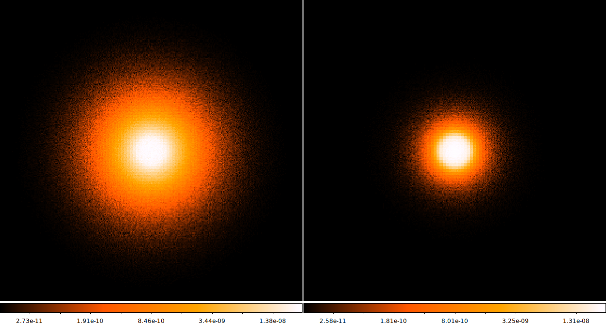
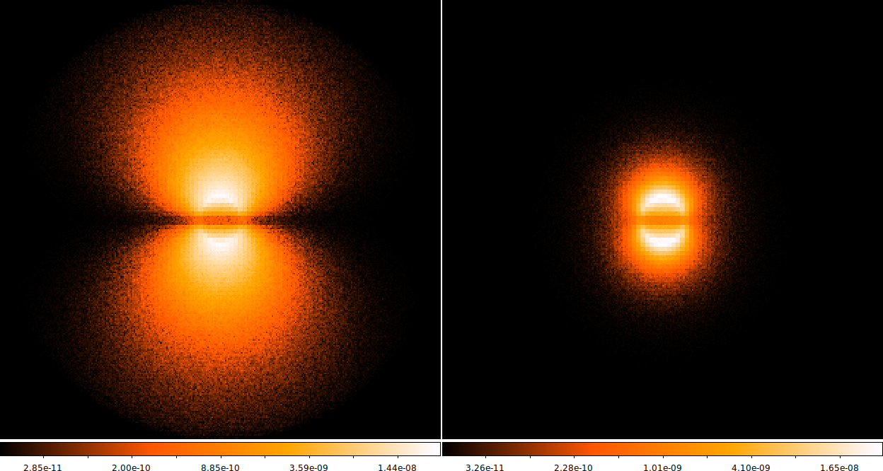
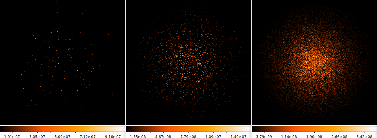
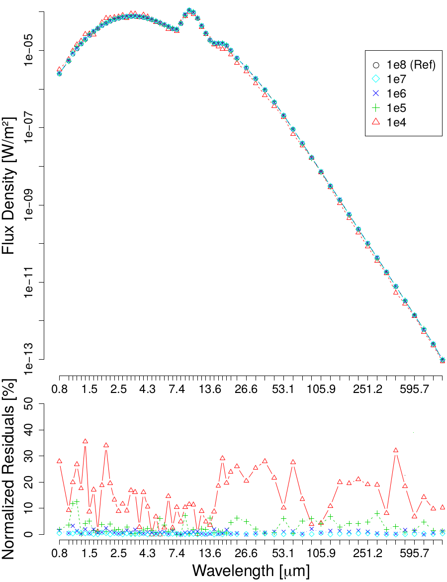
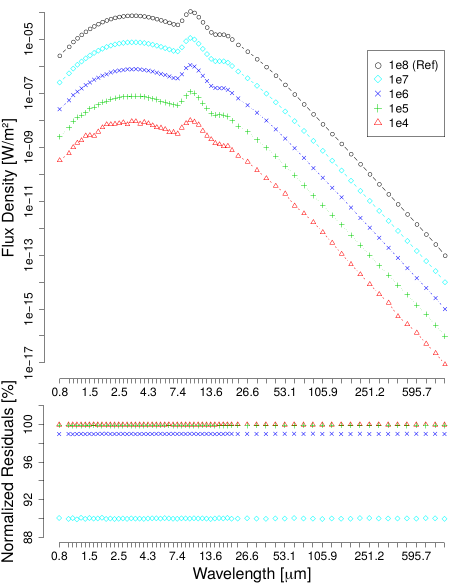
The 30 realizations differ from each other by up to three parameters: the tilt angle, $\phi$, of the object as seen by the observer ($0^{\circ}$, face-on, and $90^{\circ}$, edge-on); the optical depth, $\tau_{9.7}$, of the dust shell (0.05, 0.1 and 1.0); and the amount of photon packets simulated, $N_{p}\in\{10^{4},10^{5},10^{6},10^{7},10^{8}\}$. For each particular $\tau_{9.7}$ and $\phi$ combination the corresponding $N_{p}=10^{8}$ realization was regarded as the HPN reference, or “ground truth”, for the purpose of evaluating the performance of our routines, since those yield the highest information density, while all other simulations, with $N_{p}\in\{10^{4},10^{5},10^{6},10^{7}\}$, were considered LPN simulations. Fig. 1 illustrates the difference between HPN references through different $\tau_{9.7}$ and $\phi$ combinations, while Fig. 2 shows LPN models with differing $N_{p}$, keeping $\tau_{9.7}=0.05$ and $\phi=0^{\circ}$. Tab. 1 displays the difference between the quality of the individual spaxels that compose each LPN realization and HPN reference; the median, M, and mean absolute deviation (MAD) of the normalized residuals (see Eq. 18) of every pixel within each LPN realization; as well as the total information ratio (TIR) for all realizations, here defined as the ratio of the number of pixels with flux different than 0 of an LPN input or emulation, $N_{X^{\prime}\neq 0}$, and that same number for the HPN reference, $N_{X\neq 0}$ (see Eq. 19), as an information metric to balance against the normalized residuals:

$$Residuals(\%)=\mid\frac{X^{\prime}-X}{X}\mid\times 100\%\,\,,$$ (18)

$$TIR(\%)=\frac{N_{X^{\prime}\neq 0}}{N_{X\neq 0}}\times 100\%\,\,.$$ (19)

.

(a) $\phi=0^{\circ}$. Left: $\tau_{9.7}=0.05$; Right: $\tau_{9.7}=1.0$.

(b) $\phi=90^{\circ}$. Left: $\tau_{9.7}=0.05$; Right: $\tau_{9.7}=1.0$.

Figure 1: High photon number references of a spherical dust shell composed of silicates and graphites surrounding a bright anisotropic point source. The present flux density maps represent the simulated observations at wavelength 1,85 $\mu$m, with $\phi=0^{\circ}$ (Fig. 1(a)) and $\phi=90^{\circ}$ (Fig. 1(b)) for $\tau_{9.7}\in\{0.05,1.0\}$. Color indicates flux density in W/m².

(a) Left: $N_{p}=10^{4}$; Middle: $N_{p}=10^{5}$; Right: $N_{p}=10^{6}$.

(b) Left: $N_{p}=10^{7}$; Right: $N_{p}=10^{8}$.

Figure 2: Models of a spherical dust shell composed of silicates and graphites surrounding a bright anisotropic point source, with $\tau_{9.7}=0.05$ and $\phi=0^{\circ}$, realized by simulating different photon amounts. The present flux density maps represent the simulated observations at wavelength 9,28 $\mu$m. Fig. 2(a) presents the realization obtained by simulating $N_{p}\in\{10^{4},10^{5},10^{6}\}$, while Fig. 2(b) presents the realizations obtained by simulating $N_{p}\in\{10^{7},10^{8}\}$. Color indicates flux density in W/m².

Sim.	Normalized Residuals of Sim. (%)		Information of Simulation
	M	MAD	TIR (%)	Null Spxs ($N$)	Empty Spxs ($\Delta N$)	Full Spxs ($N$)	Partial Spxs ($N$)
$10^{4}$	100	0	0.2	82,041	64,185	0	7,959
$10^{5}$	100	0	1.9	47,964	30,108	0	42,036
$10^{6}$	100	0	15.4	19,115	1,259	0	70,885
$10^{7}$	100	59	65.2	17,904	48	2,784	69,312
$10^{8}$	0	0	100	17,856	0	47,160	24,984

Table 1: Statistics regarding how the LPN realizations compare to the HPN reference. Median normalized residuals of 100% indicate that missing information permeates the LPN realizations. The quantity and quality of the available information is further described by the total information ratio (TIR), and the amounts of different qualities of spaxels. Null spaxels are spaxels with zero information; empty spaxels are null spaxels that were not tagged as such for the HPN reference; full spaxels are spaxels that have information at every wavelength and, partial are those spaxels that are neither null nor full.

The realizations were split into two subsets: one to train the autoencoder, and perform the first batch of tests to the emulation pipeline, labeled AESet and described in Section 3.1.1; and another, comprised exclusively by data the autoencoder did not see during training, to better assess EmulARTs performance, labeled EVASet and described in Section 3.1.2.

3.1.1 AESet

This subset is comprised of 5 SKIRT simulation outputs of the same model, a spherical shell of dust composed by silicates and graphites, with optical depth $\tau_{9.7}=0.05$, surrounding a bright point source with anisotropic emission seen face-on, $\phi=0^{\circ}$, making the emission appear isotropic. The only different parameter across the realizations in AESet was $N_{p}\in\{10^{4},10^{5},10^{6},10^{7},10^{8}\}$ (see Fig. 2). The $N_{p}=10^{8}$ realization is the HPN and was used as the reference, or “ground truth”, for the purpose of both training the autoencoder model as well as evaluating the performance of EmulART.

Since the goal of our methodology is to reconstruct the reference simulation using LPN realizations as input, the values of each cube were multiplied by the ratio between the amount of photons simulated for the LPN input, $N_{p}^{LPN}$ and the amount of photons simulated for the HPN reference ($N_{p}^{HPN}=10^{8}$). In Fig. 3 we can see the impact of this de-normalization on the integrated SEDs of the LPN realizations: LPN realizations have less flux when not including SKIRTs normalization.

(a)

(b)

Figure 3: Integrated SEDs (upper panel) and normalized residuals (lower panel) for each of the five SKIRT simulations in our dataset: a) due to normalization, realizations with different amounts of photons simulated display very similar integrated SEDs; b) integrated SEDs of realizations in AESet after de-normalization (total flux is here proportional to $N_{p}$). The labels indicate the value of $N_{p}$ for each realization.

The spaxels of all cubes within AESet were used to train the DVAE model. For this we split AESet into training set (5/6) and test set (1/6). Spaxels of different cubes but which share the same spatial coordinates were assigned to the same ensemble. This strategy aimed for the DVAE model to achieve a denoising capability and consists on having input spaxels that result from realizations with different $N_{p}$ always match the HPN references version on the output layer.

In SKIRT, choosing to simulate fewer photons results in an output with more zero flux density pixels which in turn means that more spaxels will be null at more wavelength bins. Even though this is different than noise, it is akin to missing data whose impact we aim to curb by implementing a DVAE architecture.

Before training the DVAE model we perform some spaxel selection and pre-processing tasks on AESet which is thoroughly described in Appendix A.

Later, when performing preliminary tests on EmulART, we used the 4 LPN realizations within AESet ($N_{p}\in\{10^{4},10^{5},10^{6},10^{7}\}$) as input.

3.1.2 EVASet

This subset is comprised of the 25 SKIRT simulation cubes that also model a spherical shell of silicates and graphites surrounding a bright anisotropic point source but have different combinations of $\phi$, $\tau_{9.7}$ and $N_{p}$ from those in AESet. To all realizations in EVASet we performed the same feature selection and flux de-normalization tasks described both in Section 3.1.1 and Appendix A.

The 20 LPN realizations within EVASet($N_{p}\in\{10^{4},10^{5},10^{6},10^{7}\}$) were used as input for EmulART for a deeper assessment of the capabilities of our emulation pipeline. The remaining 5 HPN cubes (those with $N_{p}=10^{8}$) were used as references to compute performance metrics.

A list detailing the parameters of the SKIRT simulations used in this work, as well as their split into AESet and EVASet, can be consulted in Appendix B.

3.2 Training the DVAE

To determine which set of hyper-parameters for the DVAE suited our needs best we performed some tests, grid-searches and explored: amounts of features in the latent space; activation, loss and optimization functions; batch size; bias constraint; learning rate; and, patience values. These exploratory tests were performed by training the models during 100, 500 and 2000 epochs, according to the need to differentiate performance between hyper-parameter sets.

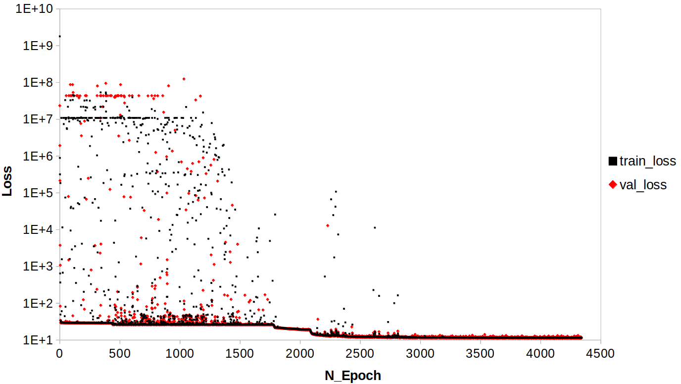
We measured performance by the percentage residuals of both the individually reconstructed spaxels, of the test subset of AESet, and of each of AESets cubes integrated SEDs. We selected the set of hyper-parameters listed below for being the most consistent across different tests. Fig. 4 shows the validation loss closely following the training loss, indicating successful convergence of the model to our data.

• Latent feature amount: 8

• Activation function: SELU (Klambauer et al, 2017) and sigmoid (for the output layer only)

• Loss function: weighted sum of the Kullback-Leibler divergence and mean percentual error

• Optimization function: Adam

• Batch size: 32

• Bias constraint: 0.95

• Train - Validation split: 4/5, 1/5

• Maximum $N_{Epoch}$: 4,500

• Patience 1: 500 epochs

• Patience 2: 3,000 epochs

• Initial learning Rate (LR): 0.001

• Learning rate decrease: 0.25

Figure 4: Loss, in log scale, as function of the number of epochs. The training loss is represented by $\blacksquare$ and the validation loss by red $\blacklozenge$. The plot shows that both metrics converge to comparable values.

After training the weights were saved to files which are loaded into the pipeline (see Section 3.3).

Appendix C shows the relationship between the compressed (or latent) features of the test set, as well as the Pearson’s correlation coefficients (PCC) between those features. Based on the analysis of the correlations of the latent features we decided to stop further compression of the spectral dimensions of the data.

3.3 DVAE Emulation Pipeline

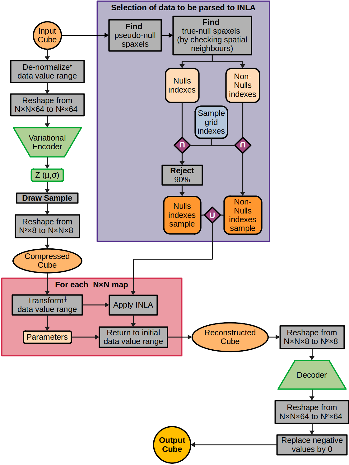
Within EmulART the feature space is first compressed with the variational encoder; the latent space is then sampled and the resulting latent features spatial maps are reconstructed with INLA; finally the reconstructed wavelength (original feature space) maps are recovered with the decoder. Additionally, to conform the data to each of the different stages of the pipeline, we perform some operations described below. Fig. 5 presents a scheme of the emulation pipeline while a flowchart including all relevant data pre- and post-processing operations, integrated within the emulation pipeline, can be found in Appendix D.

Figure 5: Scheme with the most relevant operations of the pipeline. Data shaping is represented in cyan; feature combination is in dark blue; and statistical operations are in red. Feature dimensionality is given along the axis of the arrows, at the top of each layer. $\bfmu$ is the vector holding the mean value of the latent features distribution, while $\bfsigma$ is the vector holding their variance; $\bfz$ is the vector built by randomly drawing values from the latent features distributions $G(\bfmu,\bfsigma)$.

Prior to being parsed by the encoder network module, the data is initially pre-processed as described in Appendix A. After the data goes through the encoding and variational sampling stages (see Fig. 5), the resulting latent features maps, $Z_{f}(x,y)$, are then transformed according to the following steps for each feature map, $Z_{f}(x,y)$:

1. Determine the minimum, $m^{0}_{f}$, and maximum, $M^{0}_{f}$, values of the map,

   $m^{0}_{f}=$ min$(Z_{f}(x,y)),\;\;M^{0}_{f}=$ max$(Z_{f}(x,y))$  ;

2. Determine the value range, $R_{f}$, of the map,

   $R_{f}=M^{0}_{f}-m^{0}_{f}$  ;

3. Offset the value range of the map so that the new minimum is 0,

   $Z^{\prime}_{f}(x,y)=Z_{f}(x,y)-m^{0}_{f}$  ;

4. For the offset map, $Z^{\prime}_{f}(x,y)$, determine the minimum positive value, $m^{1}_{f}$, and divide it by $R^{2}_{f}$ to obtain the new minimum , $m^{2}_{f}$,

   $m^{1}_{f}=$ min$(Z^{\prime}_{f}(x,y)):\;\;Z^{\prime}_{f}(x,y)>0$  ,

   $m^{2}_{f}=m^{1}_{f}/R^{2}_{f}$  ;

5. Obtain the final map, $Z^{\prime\prime}_{f}(x,y)$, by offsetting the value range by $m^{2}_{f}$,

   $Z^{\prime\prime}_{f}(x,y)=Z^{\prime}_{f}(x,y)+m^{2}_{f}$  .

These transformations, found by trial and error, are useful in conveying the data to INLA in a value range where its performance is both consistent (across different inference task in this scientific domain), less prone to run-time errors and more accurate. It should be noted that the validity and the improvement on performance granted by this interval transformation has only been empirically verified for our particular case, and it may well be improved upon.

After these transformations the latent features maps are reconstructed by INLA. Then they are transformed back to the original value range and are parsed by the decoder network module.

3.4 PCA Emulation Pipelines

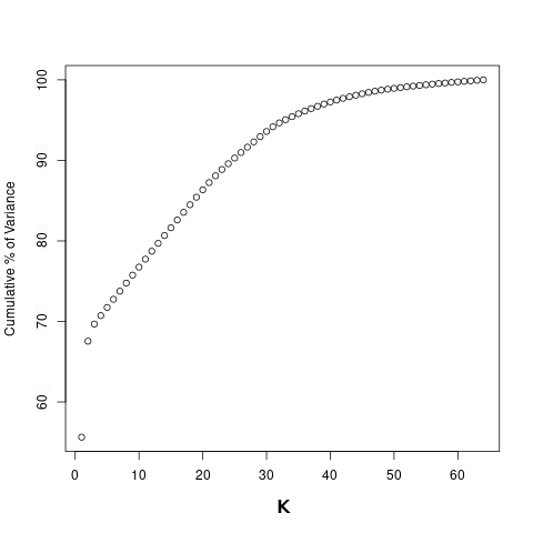
For the PCA emulation pipeline a new PCA model of the input feature space is constructed every time (unlike with the EmulART which DVAE model was trained on a subset of AESet, as described in Section 3.2). Once that model is constructed two approaches are followed: the first being the usage of the elbow method (see Fig. 6) to find the threshold number of components, K, that would explain the data without over-fitting it, using INLA to spatially reconstruct those components maps, and then return to them to the original feature space. In the second approach, 8 principal components are used (the same number as the latent features in the DVAE emulation pipeline).

Figure 6: Plot of cumulative percentage of variance explained as a function of the number of principal components, K) used to encode the data. Increasing the amount of PCs used naturally increases the percentage of variance explained but it also risks over-fitting the model. In this case the elbow can be found at around K = 30.

After some preliminary tests, the data range transformations described in the previous section, before and after spatial reconstruction, were also removed as they failed to lead to execution time or reconstruction accuracy improvement. Moreover, spaxel de-normalization (see Section 3.1.1) was removed as it lead to the underestimation of the integrated SEDs of the reference model (possible reasons for this are presented in Section 4.1.1).

A scheme presenting the most relevant operations for both implementations of the PCA emulation pipeline can be found in Appendix D.

4 Results and Discussion

In this section we present and discuss some of the results from testing EmulART on AESet, these are compared against the results obtained with the PCA emulation implementations, and EVASet. Our goal in first using AESet was to evaluate the performance of the pipeline as a whole, mostly because the decoder network was not trained on latent and INLA reconstructed spaxels. The realizations from EVASet were then used to better gauge its performance.

We created the emulations using different LPN inputs ($N_{p}\in\{10^{4},10^{5},10^{6},10^{7}\}$). Because INLA performs faster on sparse maps, for each of those LPN realizations an emulation was performed by sampling different percentages of each latent feature map. These sampling percentages resulted from sampling 1 pixel in each bin of $2\times 2$, $3\times 3$ and $5\times 5$ pixels, corresponding respectively to 25%, 11% and 4% of the spatial data. With the intent of reducing the influence of null spaxels in the spatial inference, 90% of the null spaxels were rejected from each map sampling pool.

Our analysis of the results consisted on inspecting how well EmulART reproduces the spectral and spatial features of the reference simulations, as well as the total computational time it took for the emulation to be completed.

To evaluate the spectral reconstruction we looked at the normalized residuals (see Eq. 18) between the integrated SEDs${}^{\ref{fn:iSED}}$ of our emulations and of the HPN reference. We also inspected the spatial maps of the compressed features looking for spatial distributions compatible with physical properties of the simulated model. The spatial reconstruction was also evaluated by the median and MAD of the normalized residuals of our emulations as well as of their LPN inputs at each wavelength. For the statistical analysis of the residuals, reference pixels with value 0 were not considered since this metric diverges, so the TIR for all emulations and simulations was calculated as well.

4.1 AESet Predictions

In this section we present and discuss the results obtained emulating the HPN reference of AESet using the different LPN realizations within it.

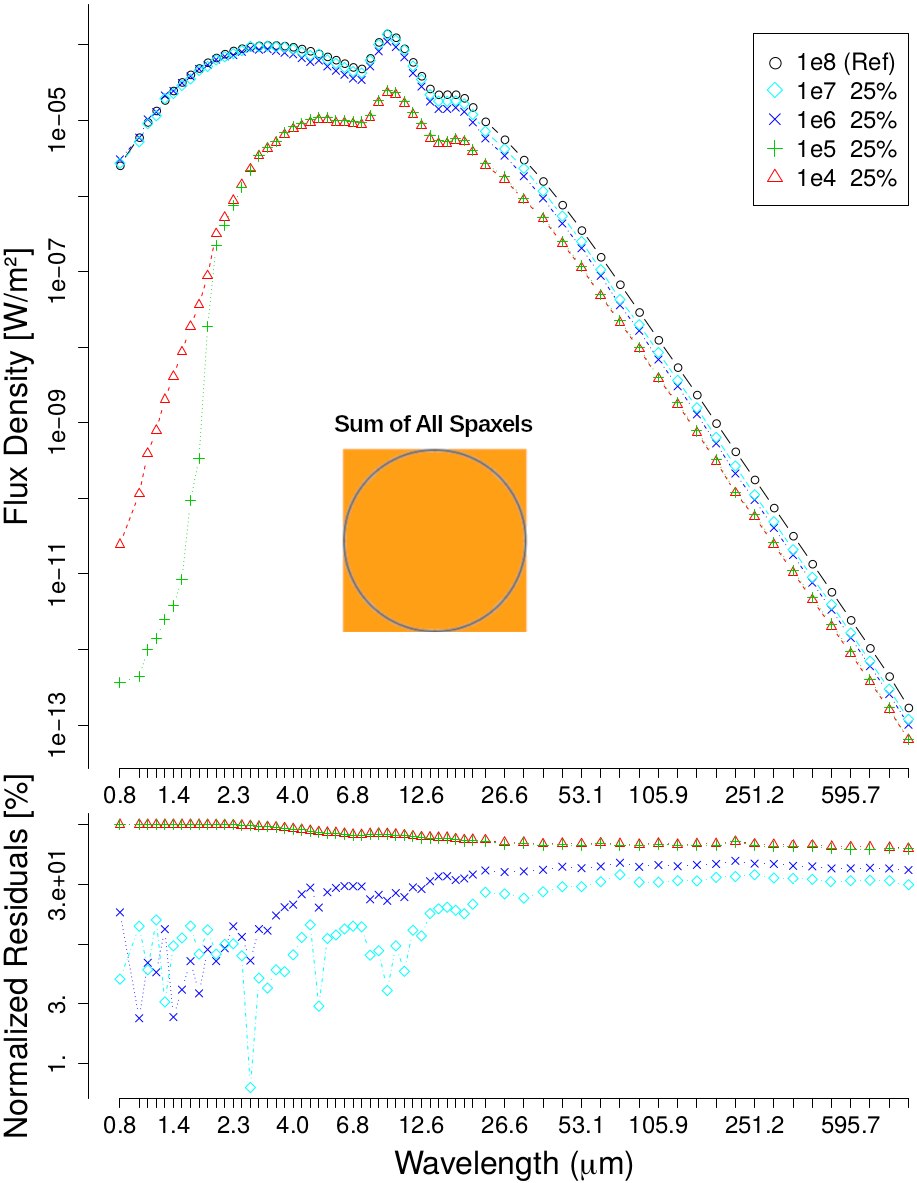
The upper panels of Fig. 7 show that the emulations integrated SEDs reproduce the shape of the references: a slow rise in the 1 $\mu$m to 8 $\mu$m range, the two emission bumps in the 8 $\mu$m to 20 $\mu$m range, and the steep decline towards longer wavelengths. Moreover, Tab. 2 displays the median and MAD of the residuals of the integrated SEDs for the LPN input realizations before and after being de-normalized (as we describe in Section 3.1.1), as well as those of the different emulations obtained from them. It is clear that using $N_{p}\geq 10^{6}$ realizations as input yields emulations integrated SEDs that closely (median residuals smaller than 15%) follow the references throughout the whole wavelength range, independently (within this subset) of the sampling percentage chosen for the spatial inference task.

(a)

(b)

(c)

Figure 7: Emulations integrated SEDs resulting from spatial inference using 4% (7(a)), 11% (7(b)) and 25% (7(c)) samples of the spatial information, and the respective normalized residuals, for the case of a dust shell with $\tau_{9.7}=0.05$ and $\phi=0^{\circ}$. The HPN reference, is represented in black ($\circ$), the emulation based on the $N_{p}=10^{4}$ realization is in red ($\triangle$), on the $N_{p}=10^{5}$ in green (+), on the $N_{p}=10^{6}$ in blue ($\times$) and on the $N_{p}=10^{7}$ in cyan ($\diamond$).

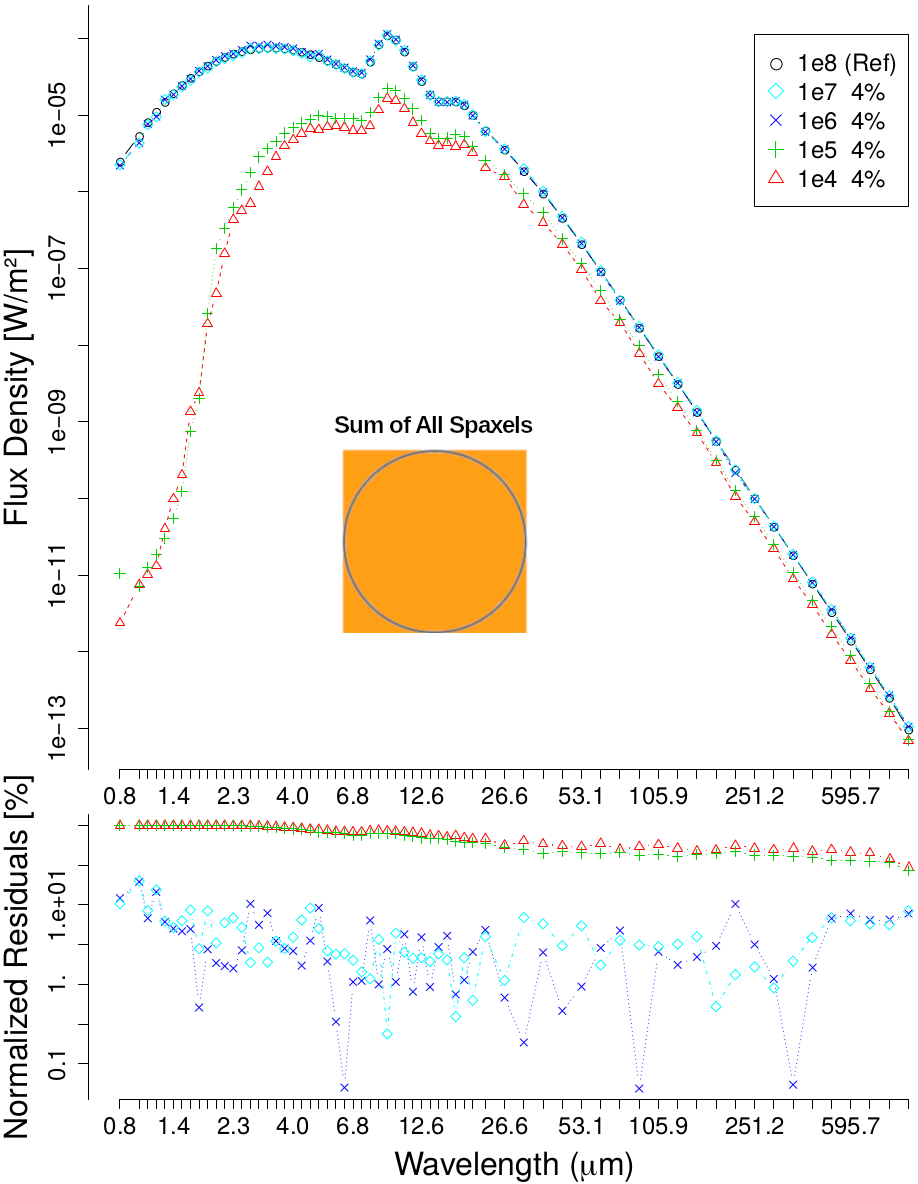
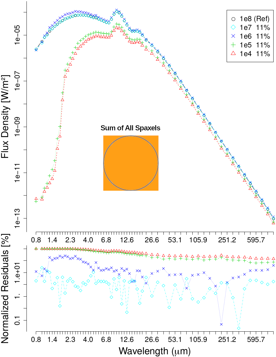
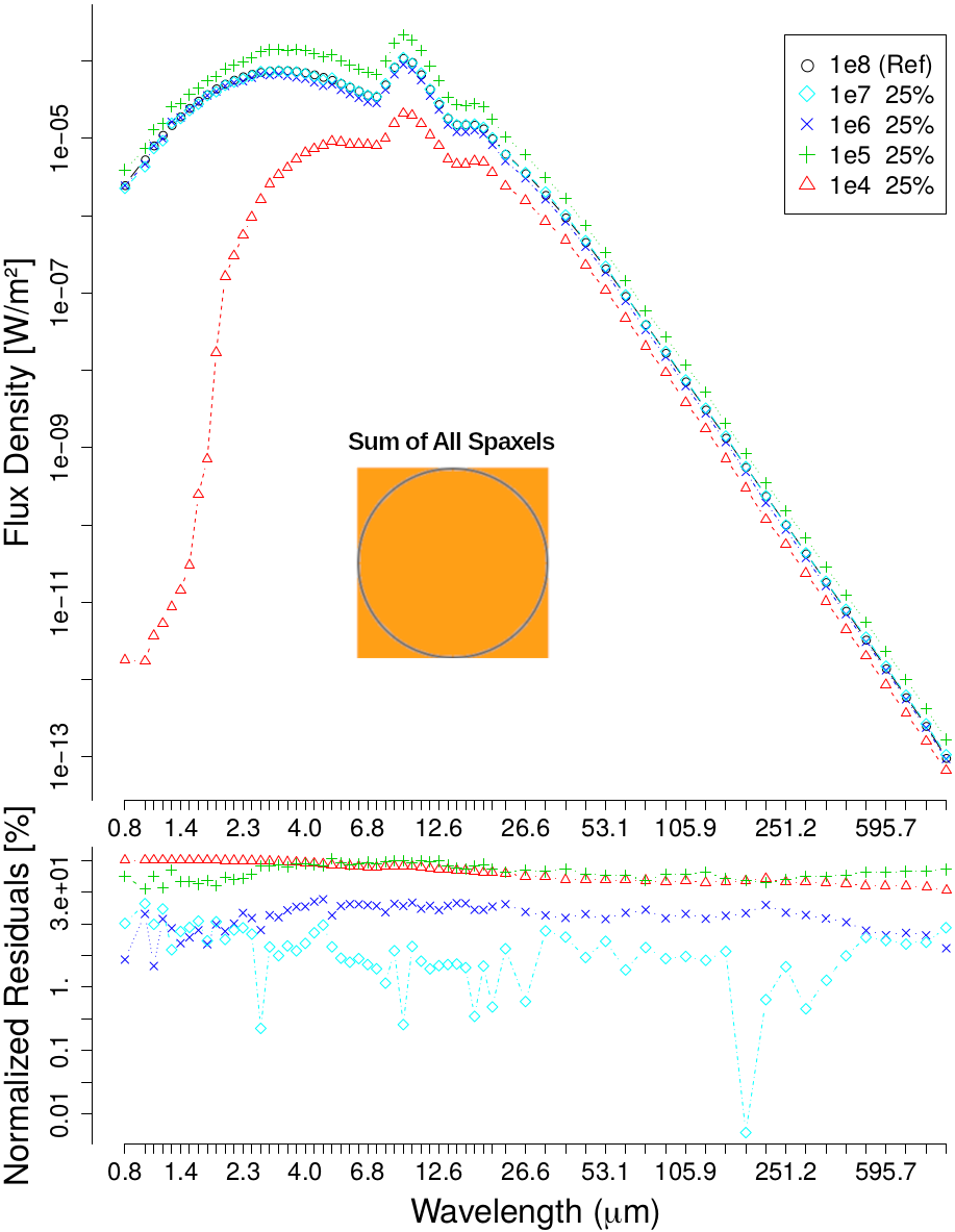
LPN Input	Residuals of Integrated Input (%)		Residuals of Integrated De-normalized Input (%)		Sample	Residuals of Integrated Emul. (%)
	M	MAD	M	MAD		M	MAD
1e4	13.4	7.4	99.99	0.00	4%	82	18
					11%	78	19
					25%	77	20
1e5	1.9	2.0	99.90	0.00	4%	75	21
					11%	68	23
					25%	67	16
1e6	0.81	0.51	99.00	0.01	4%	2.8	2.5
					11%	12	10
					25%	14.3	4.3
1e7	0.19	0.17	90.00	0.03	4%	3.3	2.4
					11%	3.6	2.0
					25%	3.8	2.7

Table 2: Comparison of statistics for the residuals of the integrated SEDs, for the case of a dust shell with $\tau_{9.7}=0.05$ and $\phi=0^{\circ}$, for the different LPN realizations (columns 2 and 3), for those same realizations but after they have been de-normalized (columns 4 and 5), as described in Section 3.1.1, and for the resulting emulations (columns 7 and 8), while using different sampling amounts (column 6) for the spatial reconstruction.

From the residuals of the emulations integrated SEDs, shown in the lower panels of Fig. 7, we conclude that: shorter wavelengths yield higher residuals; more input data for the spatial reconstruction does yield a better emulation but at the cost of an increased run time, as can be confirmed in Tab. 3; and, that the usage of the $N_{p}=10^{6}$ realization as input greatly improves the quality of the emulation in relation to the two lowest photon number alternatives.

Looking at Tabs. 1 and 3 we can also compare the overall performance of the pipeline at estimating information that was not available in the LPN input realizations. The amounts of differently classified spaxels in both LPN inputs and respective emulations show, together with median of the normalized residuals, that EmulART successfully estimates information missing from the input.

LPN Input Sample	Total Emul. Time (min)	Normalized Residuals of Emul. (%)		Information of Emulation
		M	MAD	TIR (%)	Null Spxs ($N$)	Empty Spxs ($\Delta N$)	Full Spxs ($N$)	Partial Spxs ($N$)
$10^{4}$ 4%	7.2	77	33	98.3	20,712	2,856	69,288	0
$10^{4}$ 11%	33	76	35
$10^{4}$ 25%	20	76	35
$10^{5}$ 4%	6.9	76	36	102.3	17,858	2	72,142	0
$10^{5}$ 11%	22	75	37
$10^{5}$ 25%	19	196	272
$10^{6}$ 4%	8.9	42	45	103.6	16,969	-887	73,031	0
$10^{6}$ 11%	25	40	45
$10^{6}$ 25%	26	48	45
$10^{7}$ 4%	7.6	31	32	103.7	16,866	-990	73,134	0
$10^{7}$ 11%	31	32	33
$10^{7}$ 25%	19	26	26

Table 3: Statistics regarding how the different emulations, of the case of a dust shell with $\tau_{9.7}=0.05$ and $\phi=0^{\circ}$, compared to the HPN reference. The median normalized residuals and TIR display great improvement against all LPN realizations (see Tab. 1). The emulations that used $N_{p}=10^{6}$ and $N_{p}=10^{7}$ realizations as input display a negative amount of empty spaxels, indicating that beyond reconstructing all empty spaxels it also inferred some of the references nulls.

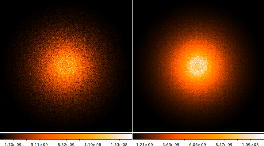
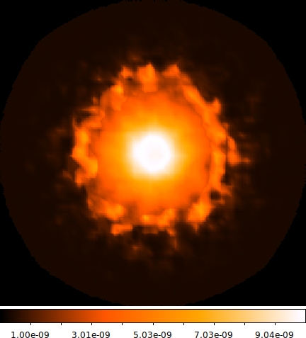
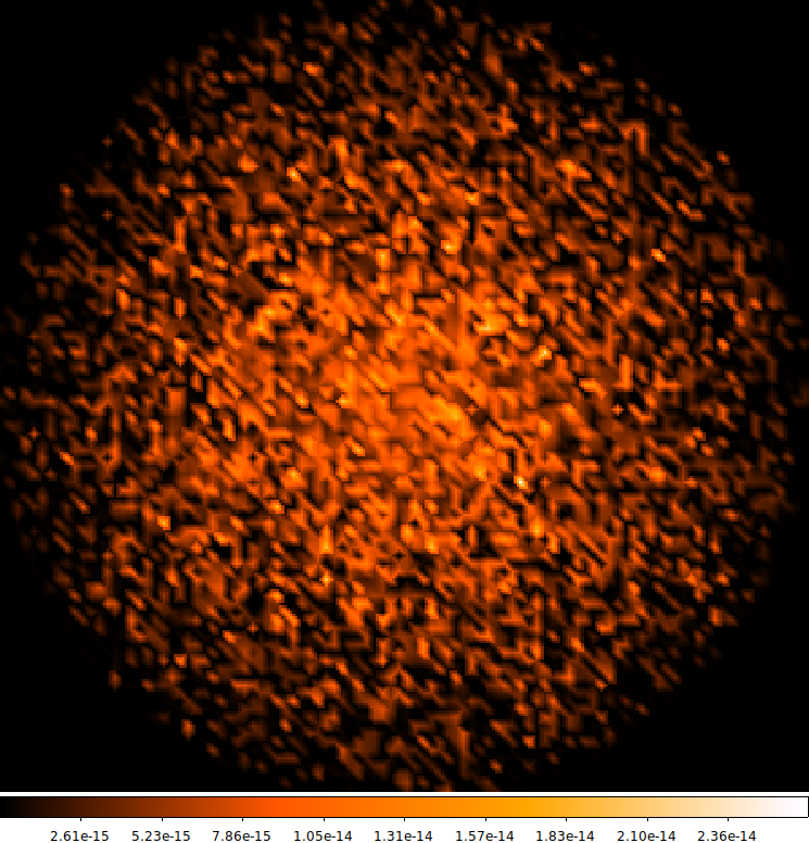
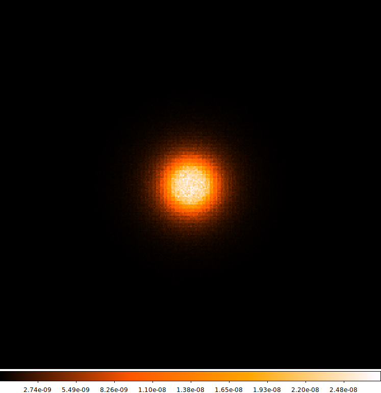
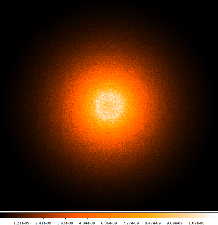
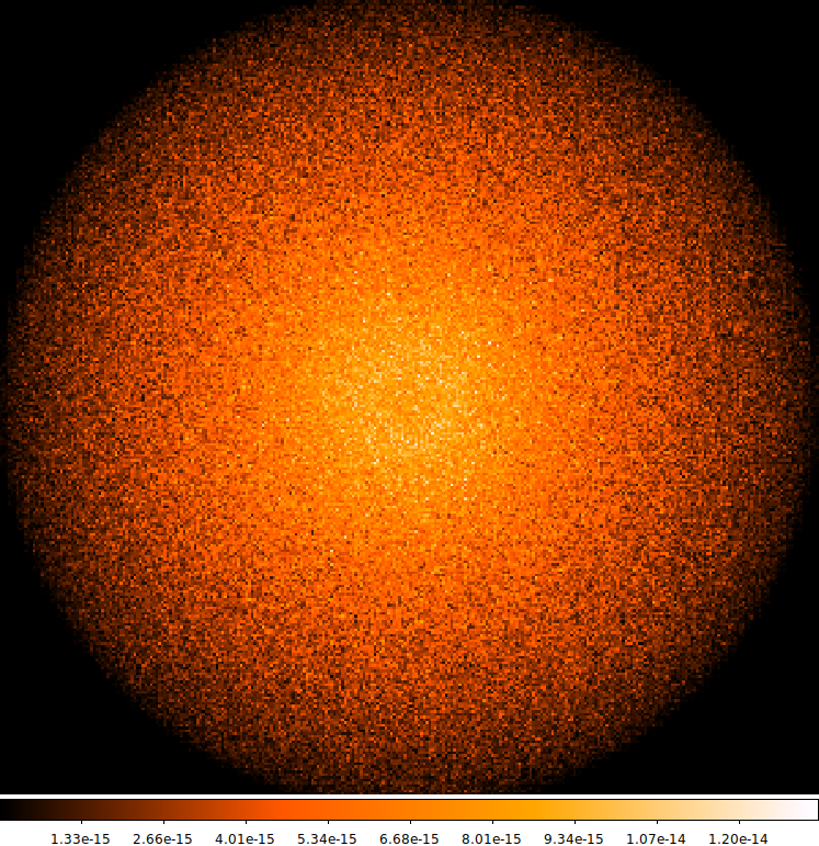
Fig. 8 shows the comparison, at wavelength 9.28 $\mu$m, between the emulations resulting from the LPN inputs (see Fig. 2) and the HPN reference. Once again we can see that with the $N_{p}=10^{6}$ realization the emulations start to display resemblances to the HPN reference not only in the range of flux density values but also in the morphology that emerges from their distribution.

(a)

(b)

(c)

Figure 8: Spatial maps of emulations, of the case of a dust shell with $\tau_{9.7}=0.05$ and $\phi=0^{\circ}$, at wavelength 9.28 $\mu$m, based on the input of 4% of $N_{p}=10^{6}$ LPN realization spatial information (Fig. 8(a)), 4% of $N_{p}=10^{7}$ LPN realization spatial information (Fig. 8(b)) and the HPN reference (Fig. 8(c)). Color indicates flux density in W/m².

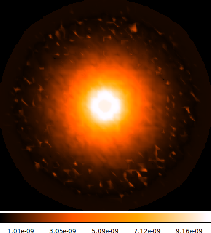
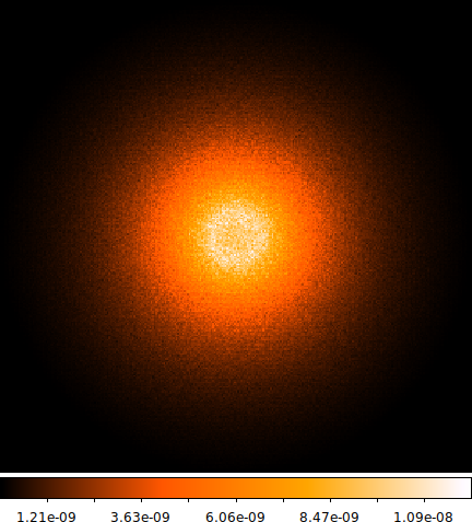
From Tabs. 2 and 3, as well as from Figs. 7 and 8, it would be natural to conclude that using the $N_{p}=10^{7}$ realization as input would bring the most benefit in terms of the amount of information inferred by the emulation as well as its accuracy. Moreover, as can be seen in the second column of Tab. 3, the run time of the emulations is more dependent on the amount of information sampled for the spatial reconstruction than on the $N_{p}$ of the LPN input. Nevertheless, considering how SKIRTs run time for a model scales with the simulated $N_{p}$, the choice of LPN input to use with EmulART should weight the time it takes to produce that LPN input as well as the quality of the emulation we expect from it.

4.1.1 PCA Pipeline Predictions

The results of testing the PCA pipelines on AESet were processed in the same way as EmulARTs (statistical indicators regarding residuals of the emulation and of its spatial integration were calculated as well as the TIR; the number of different types of spaxels and execution time were measured).

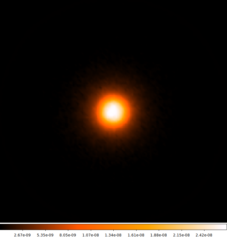
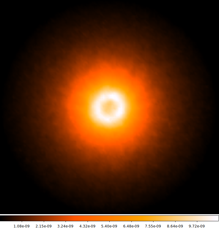
The execution times for the pipeline implementing an 8 PC model were indiscernible from the execution times of EmulART on the same input, while the execution time for the pipeline implementing a PCA model with number of components, K, determined by the elbow method was in general much higher since for all except one of the LPN inputs K was larger than 30 (the time per component map was very similar depending mostly on the amount of spatial information sampled).

Tabs. 4 and 5 present the most significant indicators to be compared to EmulARTs. At first sight the performance of both PCA models on the emulation pipeline seems to be similar to, and in some cases even better than that of EmulARTs, showing statistically similar residuals, and presenting residuals regarding the spatially integrated SEDs  2 to 3 times lower. They are however unable to consistently recover complete spaxel information which then leads to poor spatial reconstructions at longer wavelengths, even when using K $>$ 8 (see Fig. 9), as can be inferred from the TIR values (as well as the number of full and partial spaxels).

(a)

(b)

(c)

(d)

(e)

(f)

Figure 9: Spatial maps of emulations (Top), performed with a pipeline including a PCA model with K = 30 components based on the input of 11% of the spatial information of the $N_{p}=10^{7}$ LPN realization; and, reference simulation (Bottom) of the case of a dust shell with $\tau_{9.7}=0.05$ and $\phi=0^{\circ}$, at wavelengths 1.85 $\mu$m (Figs. 9(a) and 9(d)), 9.28 $\mu$m (Figs. 9(b) and 9(e)) and 211.35 $\mu$m (Figs. 9(c) and 9(f)). Color indicates flux density in W/m².

Input	K	Normalized Residuals of Emul. (%)	Residuals of Integrated Emul. (%)		Information of Emulation
		M	M	MAD	TIR (%)	Null Spxs ($N$)	Empty Spxs ($\Delta N$)	Full Spxs ($N$)	Partial Spxs ($N$)
$0^{\circ}$, $10^{4}$	55	100	63	54	53	20712	2856	0	69288
$0^{\circ}$, $10^{5}$	64	99	13	13	70	17858	2	10589	61553
$0^{\circ}$, $10^{6}$	48	99	3	3	77	17051	-805	2458	70491
$0^{\circ}$, $10^{7}$	31	52	1	2	86	16866	-990	3820	69314
$90^{\circ}$, $10^{4}$	8	97	25	44	66	20497	2641	0	69503
$90^{\circ}$, $10^{5}$	55	100	18	19	60	18002	146	0	71998
$90^{\circ}$, $10^{6}$	48	98	3	4	75	16872	-984	1322	71806
$90^{\circ}$, $10^{7}$	40	48	1	2	90	16833	-1023	9346	63821

Table 4: Statistics regarding PCA pipeline emulations, using K PCs (where K was determined by the elbow method) of the case of a dust shell with $\tau_{9.7}=0.05$, $\phi\in\{0^{\circ},90^{\circ}\}$ and spatial sampling of 11%.

Input	Normalized Residuals of Emul. (%)	Residuals of Integrated Emul. (%)		Information of Emulation
	M	M	MAD	TIR (%)	Null Spxs ($N$)	Empty Spxs ($\Delta N$)	Full Spxs ($N$)	Partial Spxs ($N$)
$0^{\circ}$, $10^{4}$	96	24	52	73	20712	2856	0	69288
$0^{\circ}$, $10^{5}$	100	22	15	75	17858	2	3127	69015
$0^{\circ}$, $10^{6}$	64	4	6	84	17051	-805	2352	70597
$0^{\circ}$, $10^{7}$	33	1	2	88	16866	-990	3122	70012
$90^{\circ}$, $10^{4}$	97	25	44	66	20497	2641	0	69503
$90^{\circ}$, $10^{5}$	100	20	13	70	18002	146	151	71847
$90^{\circ}$, $10^{6}$	55	2	5	85	16872	-984	2884	70244
$90^{\circ}$, $10^{7}$	30	1	2	91	16833	-1023	6845	66322

Table 5: Statistics regarding PCA pipeline emulations, using 8 PCs, of the case of a dust shell with $\tau_{9.7}=0.05$, $\phi\in\{0^{\circ},90^{\circ}\}$ and spatial sampling of 11%.

In the present application we thus find the implementation of a DVAE model for spectral compression to be justified. Unlike the PCA models, it not only captures non-linear relationships between the spectral features but also achieves comparable results. Despite some loss regarding the reconstruction of integrated SED profile, when compared to PCA models, it achieves equal/higher compression rate, lower/equal execution time and most importantly the spatial structure can successfully be reconstructed by the remaining parts of the pipeline.

As such, the test results of EmulART on EVASet are compared against its results on AESet. Testing results obtained with PCA emulation pipelines on EVASet did not offer a perspective different from the one above and as such will not be discussed further here (a successful implementation of PCA in an emulation pipeline is described in Smole et al (2022, submitted)).

4.2 EVASet Predictions

In this section we present and discuss the results obtained by emulating the HPN references of EVASet using the respective LPN realizations within it. The DVAE model was not trained on any data within this set, which allows us to evaluate whether it manages to accurately predict HPN-like spaxels from LPN spaxels that originate from simulations with different $\tau_{9.7}$ and $\phi$ values.

First we tested EmulART on realizations with $\tau_{9.7}=0.05$ and $\phi=90^{\circ}$; we then applied the pipeline to different LPN realizations with $\tau_{9.7}\in\{0.1,1.0\}$ and $\phi\in\{0^{\circ},90^{\circ}\}$.

Similarly to the $\tau_{9.7}=0.05$ and $\phi=0^{\circ}$ emulations, the edge-on, $\phi=90^{\circ}$, emulations appear to preserve well the spectral information, reproducing the slow rise in the 1 $\mu$m to 8 $\mu$m range, the two emission bumps in the 8 $\mu$m to 20 $\mu$m range, and the steep decline towards longer wavelengths, as can be seen in Fig. 10. Tab. 6 shows that 4% sampling of the spatial information of the $N_{p}=10^{6}$ realization is enough to get median integrated residuals below 15%. We note however the abnormal performance of the emulations that took as input the $N_{p}=10^{7}$ realizations, displaying higher median integrated residuals than the ones that used different samplings of the $N_{p}=10^{6}$ LPN. This may indicate that one or more of the spatial data manipulation modules, or their interface, should be improved upon.

(a)

(b)

(c)

Figure 10: Emulations integrated SEDs, resulting from spatial inference using 4% (10(a)), 11% (10(b)) and 25% (10(c)) samples of the spatial information, and the respective normalized residuals, for the case of a dust shell with $\tau_{9.7}=0.05$ and $\phi=90^{\circ}$. The HPN reference is represented in black ($\circ$), the emulation based on the $N_{p}=10^{4}$ realization is in red ($\triangle$), on the $N_{p}=10^{5}$ in green (+), on the $N_{p}=10^{6}$ in blue ($\times$) and on the $N_{p}=10^{7}$ in cyan ($\diamond$) .

LPN Input	Residuals of Integrated Input (%)		Residuals of Integrated De-normalized Input (%)		Sample	Residuals of Integrated Emul. (%)
	M	MAD	M	MAD		M	MAD
1e4	13.4	7.4	99.99	0.00	4%	77	19
					11%	16	19
					25%	78	19
1e5	1.9	2.0	99.90	0.00	4%	76	20
					11%	71	23
					25%	63	25
1e6	0.83	0.51	99.00	0.01	4%	13.2	7.4
					11%	46	41
					25%	13.1	5.0
1e7	0.19	0.17	90.00	0.03	4%	23.7	5.7
					11%	22.7	5.7
					25%	19.6	4.9

Table 6: Comparison of statistics for the residuals of the spatial integration SEDs, for the case of a dust shell with $\tau_{9.7}=0.05$ and $\phi=90^{\circ}$, for the different LPN realizations (columns 2 and 3), for those same realizations but after they have been de-normalized (columns 4 and 5), as described in Section 3.1.1, and for the resulting emulations (columns 7 and 8).

As for the emulations using as input LPN realizations of simulations with $\tau_{9.7}\in\{0.1,1.0\}$, at both tilt angles, we observe that both the shape and flux density value range of the integrated SED degrades as $\tau_{9.7}$ increases. As shown in Fig. 11, the emulations integrated SEDs fail to reproduce the shape of the HPN references, reproducing instead the shape that characterized the realizations present in AESet, a clear sign of over-fitting of the DVAE model. This can be solved by expanding the training set of our DVAE architecture to include spaxels originating from simulations with different optical depths.

(a) $\phi=90^{\circ}$

(b) $\phi=0^{\circ}$

Figure 11: Emulations integrated SEDs, resulting from spatial inference using 25% of spatial information, and the respective normalized residuals, for the case of a dust shell with $\tau_{9.7}=1.0$, $\phi=90^{\circ}$ (Fig. 11(a)) and $\phi=0^{\circ}$ (Fig. 11(b)). The HPN reference is represented in black ($\circ$), the emulation based on the $N_{p}=10^{4}$ realization is in red ($\triangle$), on the $N_{p}=10^{5}$ in green (+), on the $N_{p}=10^{6}$ in blue ($\times$) and on the $N_{p}=10^{7}$ in cyan ($\diamond$) .

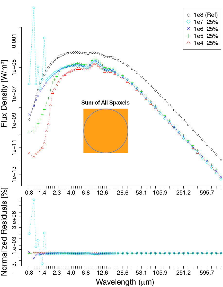
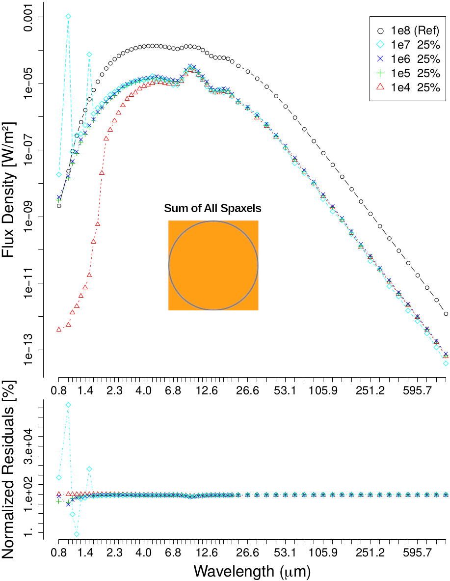
For $\tau_{9.7}=1.0$, with both $\phi$ cases, we observe the influence of the first wavelengths (see Fig. 12) in the overall residuals. Fig. 13 shows that though the overall morphology of the spatial distribution is well recovered the value range for the emulations flux density value range is drastically underestimated while the contrast between the central and peripheral regions is considerably higher than what the HPN references display.

(a) $\phi=0^{\circ}$

(b) $\phi=90^{\circ}$

Figure 12: Median of the normalized residuals, at each wavelengths spatial map, for every emulation obtained with $N_{p}=10^{4}$ (red), $N_{p}=10^{5}$ (green), $N_{p}=10^{6}$ (blue) and $N_{p}=10^{7}$ (cyan) realizations, for the case of a dust shell with $\tau_{9.7}=1.0$, with $\phi=0^{\circ}$ (Fig. 12(a)) and $\phi=90^{\circ}$ (Fig. 12(b)). Emulations whose spatial inference was performed using 25% of data are represented by ($\triangle$), 11% by (+) and 4% by ($\times$). The interrupted black line marks the same metric for the LPN inputs.

(a) $\phi=0^{\circ}$

(b) $\phi=90^{\circ}$

Figure 13: Emulation produced using as input a 25% sample of the $N_{p}=10^{6}$ realization (left panel) and HPN reference (right panel) at wavelength 9.28 $\mu$m, for the case of a dust shell with $\tau_{9.7}=1.0$, $\phi=0^{\circ}$ (Fig. 13(a)) and $\phi=90^{\circ}$ (Fig. 13(b)).

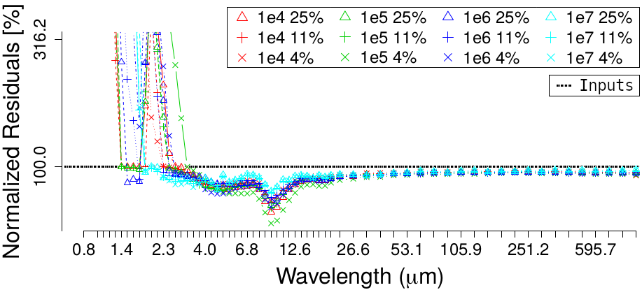
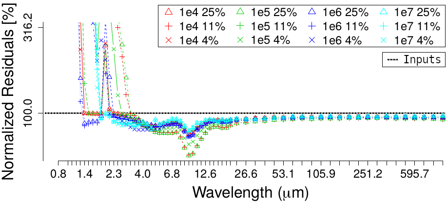
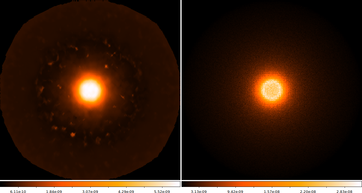
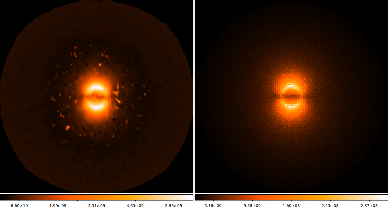
These results appear to show that our pipeline is capable of recovering $40\%$ to $60\%$ of the emergent spatial information of HPN MCRT models from LPN realizations, taking as input as little as 0.04% of the information that would be present in the HPN model, all while preserving $85\%$ to $95\%$ of the spectral information.

Furthermore the results also show a clear bias in the performance of the DVAE model as a compressor and decompressor of spectral information, with the performance degrading substantially as the LPN inputs models depart from the optical depth, $\tau_{9.7}$, value present within the training set.

Further details of the results we obtained with AESet and EVASet are discussed in Appendix E.

5 Summary

We report the development of a pipeline that implements in conjunction a denoising variational autoencoder (or alternatively PCA), and a reconstruction method based on approximate Bayesian inference, INLA, with the purpose of emulating high information-like MCRT simulations using LPN MCRT models, created with SKIRT, as input. With this approach we aim for the hastily expansion of libraries of synthetic models against which to compare future observations. By producing positive preliminary indicators we show that such a framework is worth pursuing further, with multiple alleys to explore.

Conditions for systematically measuring the computational cost are necessary to properly evaluate the merit of this approach. However, in this work our aim was to qualitatively assess the potential of this method to be applied to MCRT simulations images. In this pilot study we chose a very simple model of a centrally-illuminated spherical dust shell which is computationally inexpensive, whose reference simulations took around two hours to be computed. Thus, in our particular examples we reduced the computational time by approximately 6$\times$. Nevertheless, the computational cost of SKIRT simulations scales with the amount of photon packets simulated, the spatial resolution of the grid and the actual geometrical complexity of the model. As for our emulation pipeline, its computational cost is only impacted noticeably when increasing the size and density of the spatial grid to be processed by INLA. This leads us to believe that a generalized version of this pipeline may expedite, by up to 50$\times$, the study of dust environments through this kind of radiative transfer models.

Further exploration of the proposed DVAE architecture is being undertaken, via expansion and diversification of the training set to improve the prediction of the spectral features.

Other approaches to be tested include the use of dropout (cutting the connections, mid training, whose weights are below a given threshold) and incremental learning (training a model with new data with the starting point of the network being the weights obtained in a previous training session). The first serves as feature selection tool, removing those of little importance, which also prevents the model from over-fitting the training data; the second would be of great use to quickly adapt an already trained model to new data, which is important in the context of emulating simulations.

To improve the reconstruction of the spatial features, using non-uniform sampling methods based on the information spatial density may help improve the reconstruction of the latent features that result from the compression of models simulated with insufficient number of photon ($N_{p}<10^{6}$, in the particular case of our study). Alternative pre-INLA data pre-processing, such as data value range manipulations and sampling grids, may also be worth exploring.

Acknowledgments Computations were performed at the cluster “Baltasar-Sete-Sóis” and supported by the H2020 ERC Consolidator Grant “Matter and strong field gravity: New frontiers in Einstein’s theory” grant agreement no. MaGRaTh-646597.

J. R.-S. is funded by Fundação para a Ciência e a Tecnologia (https://www.fct.pt/) (PD/BD/150487/2019), via the International Doctorate Network in Particle Physics, Astrophysics and Cosmology (https://idpasc.lip.pt/). The work here described is integrated in the CRISP project, which is also funded by the FCT (PTDC/FIS-AST/31546/2017). M.S. and M.S. acknowledge support by the Ministry of Education, Science and Technological Development of the Republic of Serbia through the contract no. 451-03-9/2021-14/200002 and by the Science Fund of the Republic of Serbia, PROMIS 6060916, BOWIE.

Declarations

The authors declare no conflict of interest. The founding sponsors had no role in the design of the study; in the collection, analyses, or interpretation of data; in the writing of the manuscript, and in the decision to publish the results.

Appendix A Data Pre-processing

A.1 Identifying and Sampling Null-Spaxels

The SKIRT simulations of the spherical simulated models result in a peripheral region filled with spaxels with value 0 at all wavelength bins, these will be henceforth be referred to as null-spaxels. We perform two routines to identify and filter out null-spaxels, to curb their potential impact in both training the DVAE model and when (within the emulation procedure) reconstructing the spatial information of the latent feature maps:

1. Each feature (wavelength) of each spaxel is checked, if all features of a spaxel have value 0, then that spaxel is temporarily tagged as null-spaxel;

2. An iterative process then checks the immediate neighborhood of each previously tagged spaxel (a 5pix$\times$5pix grid centered at the spaxel being tested) for other tagged spaxels, if a minimum of 4 neighbors share the null-spaxel tag, then that spaxel is tagged as a true null-spaxel, otherwise its temporary tag is removed.

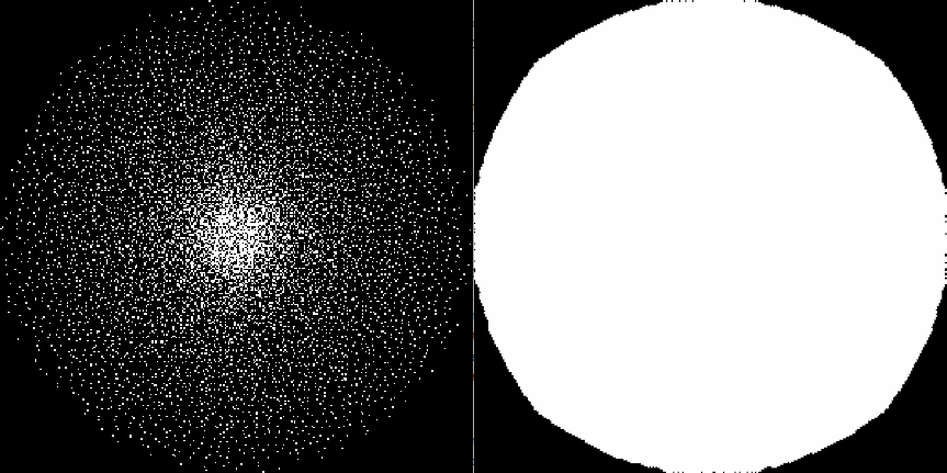
The second routine serves as a way to discriminate spaxels that have zero information at given wavelengths, possibly from the spaxel being the result of a low photon count simulation, from actual null-spaxels - spaxels resulting from the lack of photons traveling from the source to the observer through that direction, neither by direct emission nor by scattering nor by absorption and re-emission by dust. Fig. 14 illustrates the results of routine 1 and 2.

Figure 14: On the left, in black, the spaxels temporarily tagged as null-spaxels by routine 1; on the right, also in black, the final selection of null-spaxels that resulted from applying routine 2 with a search grid of 5pix$\times$5pix around each temporary null-spaxel. The result on the right shows that for this particular case of a spherical shell of dust surrounding an isotropic emitter we only find null-spaxels on the outskirts of the shell, as expected.

After identifying the null-spaxels we sample them to incorporate the filtered dataset.

For the DVAE training, complete removal of these null-spaxels could be done but we decided to reduce their incidence rate instead. Since there is no guarantee that their latent representation (where the spatial reconstruction will take place) will also be a null-vector we want the DVAE model to learn null-spaxels, too many of these will nevertheless be uninformative and may lead to unintended biases. For this reason we sample 10% of them, reducing the null-spaxel prevalence in the training dataset from $\sim$25% to $\sim$2.5%. Empty spaxels (spaxels tagged as null for LPN realizations but non-null for the respective HPN reference) were completely removed from training.

For the emulation process, and more specifically for the spatial reconstruction of the latent feature maps, we sample 10% of the null-spaxels selected by the spatial sampling grid, for INLA is faster with little data and that amount is sufficient for the null-region to be properly recovered. After the emulation process, spaxels that were at this stage identified as being null-spaxels have their values changed to 0.

A.2 Reshaping Data Structures

Once all spaxels are selected the data cubes are reshaped into a 2D structure, with a given pixel corresponding to a row with its spectral information on the columns (see Fig. 5), to match the input format of the DVAE. The inverse reshaping, from a 2D to a 3D structure, is performed after the DVAE output layer.

Within the emulation pipeline the data is reshaped two more times. First, after sampling the latent feature distributions (to obtain the $Z$ arrays, as seen in Fig. 5) the resulting sample is reshaped from a 2D to a 3D structure to obtain latent feature spatial maps (the 8 1D arrays become 8 2D maps) whose spatial information can then be reconstructed with INLA. The second reshape is performed on INLAs reconstructed results to conform that data to the decoder accepted input format, once again going from a 3D to a 2D structure.

Appendix B Dataset

Tab. 7 presents the list of SKIRT simulations used in this work. Every realization models a spherical dust, composed by silicates and graphites, surrounding a bright point source with anisotropic emission, differing in parameters such as the tilt angle, $\phi$, the optical depth, $\tau_{9.7}$, and the amount of photon packets simulated, $N_{p}$.

$N$	$\tau_{9.7}$	$\phi$ (deg)	$N_{p}$	Subset
1	0.05	0	$10^{4}$	AESet
2	0.05	0	$10^{5}$	AESet
3	0.05	0	$10^{6}$	AESet
4	0.05	0	$10^{7}$	AESet
5*	0.05	0	$10^{8}$	AESet
6	0.05	90	$10^{4}$	EVASet
7	0.05	90	$10^{5}$	EVASet
8	0.05	90	$10^{6}$	EVASet
9	0.05	90	$10^{7}$	EVASet
10*	0.05	90	$10^{8}$	EVASet
11	0.1	0	$10^{4}$	EVASet
12	0.1	0	$10^{5}$	EVASet
13	0.1	0	$10^{6}$	EVASet
14	0.1	0	$10^{7}$	EVASet
15*	0.1	0	$10^{8}$	EVASet
16	0.1	90	$10^{4}$	EVASet
17	0.1	90	$10^{5}$	EVASet
18	0.1	90	$10^{6}$	EVASet
19	0.1	90	$10^{7}$	EVASet
20*	0.1	90	$10^{8}$	EVASet
21	1.0	0	$10^{4}$	EVASet
22	1.0	0	$10^{5}$	EVASet
23	1.0	0	$10^{6}$	EVASet
24	1.0	0	$10^{7}$	EVASet
25*	1.0	0	$10^{8}$	EVASet
26	1.0	90	$10^{4}$	EVASet
27	1.0	90	$10^{5}$	EVASet
28	1.0	90	$10^{6}$	EVASet
29	1.0	90	$10^{7}$	EVASet
30*	1.0	90	$10^{8}$	EVASet

Table 7: Parametrical description of the SKIRT realizations used in this work, along with the distribution of these realizations by subset. Realizations marked with (*) were not parsed as input to EmulART while testing the pipeline, being used merely as the HPN reference for the purpose of computing performance metrics.

Appendix C Latent Features

In this section we briefly discuss the relationship between each of the compressed features, as well as how they may relate to some physical attributes of the simulated models.

The PCC measures how strongly linearly correlated different parameters are, and is defined as the ratio between the covariance of the parameters and the product of their standard deviations (see Eq. 20):

$$\rho_{X,Y}=\frac{cov(X,Y)}{\sigma_{X}\sigma_{Y}}\,\,.$$ (20)

Fig. 1 illustrates the relationships between our datasets latent features along with their respective PCC. The PCC indicates that only the first feature shows little correlation with the others, ranging from -0.42 to 0.39, while the remaining features display high correlations (and anti-correlations) between themselves, most either above 0.9 or below -0.8. This would indicate that the information in those features presents a high level of redundancy.

The point spread in the panels of Fig. 1 shows, however, something unexpected given the PCC values. There are clearly distinct populations, some presenting linear behavior, while others show highly non-linear relationships (see, for example, Z3 vs Z5) and even dual linear populations (see Z6 vs Z7).

The overall large Pearson correlation values thus indicate that the population density within the linear spreads is higher. But even if the compressed features show at best linear correlations (and anti-correlations) for a greater fraction of our data, we decided not to ignore the non-linear behavior being expressed for the remaining data. In future implementations we will tackle this by both expanding the dataset, including models with different dust distributions and compositions and employing different training strategies (this can be achieved by changing loss function terms and adding different training stages).

Figure 1: Corner plot of the latent features, $Z_{f}$ of the test set. Pearson’s correlation coefficients are indicated in navy blue.

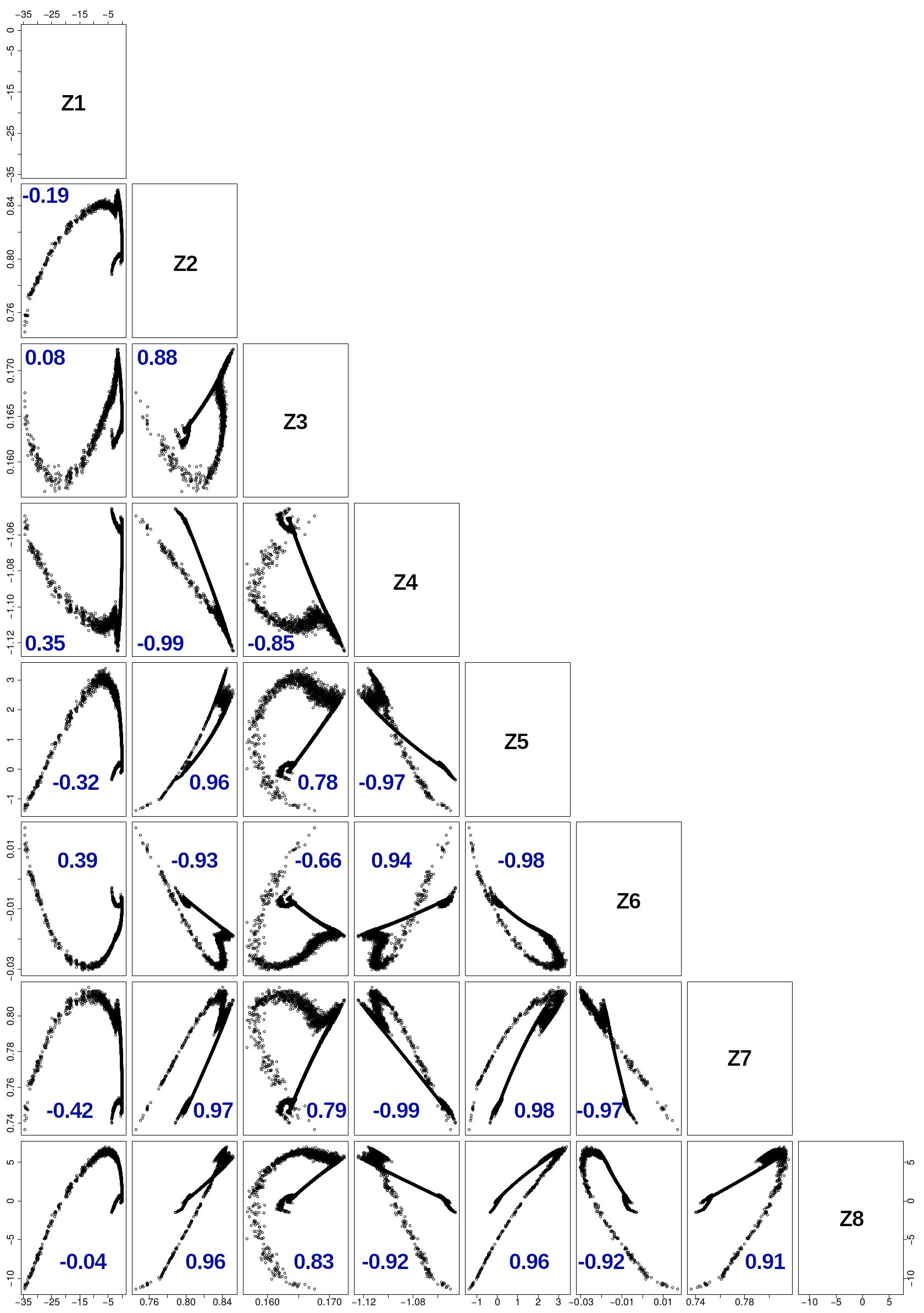
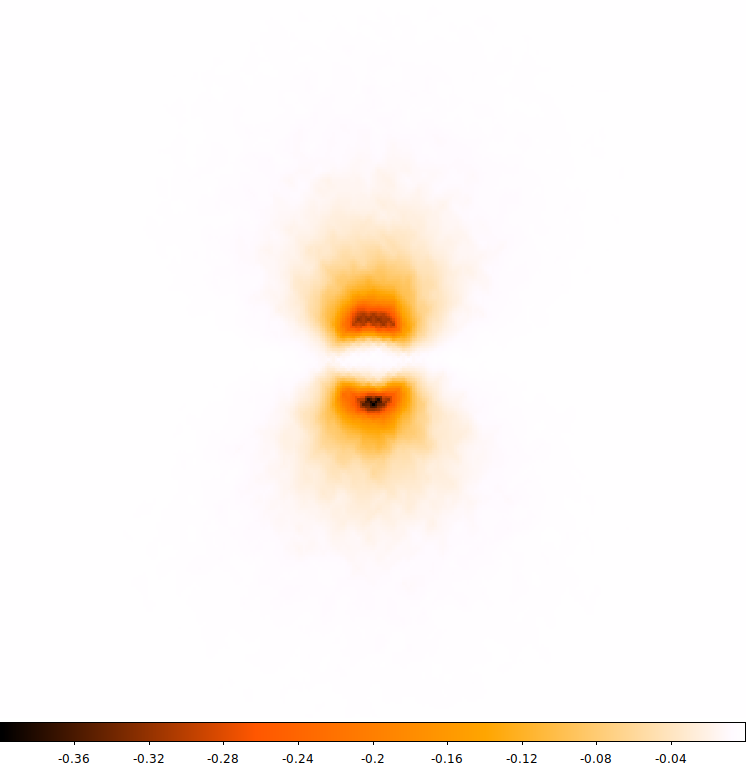
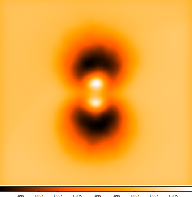
Fig. 2 shows the spatial reconstruction of 3 latent feature maps obtained from the $N_{p}=10^{6}$ LPN realization of the case of a dust shell with $\tau_{9.7}=0.05$ and $\phi=90^{\circ}$.

In the map of latent feature Z1 (Fig. 2(a)) we can relate the spatial distribution to the hot dust emission, at wavelengths 1-3$\mu$m, of the region close to the sublimation zone around the central source. Conversely, in the map of latent feature Z2 (Fig. 2(b)), the larger structure further away form the center, which corresponds to the colder dust emission at longer wavelengths is outlined.

(a) Z1

(b) Z2

(c) Z8

Figure 2: Spatial reconstruction of 3 latent feature maps of the LPN case $N_{p}=10^{6}$, $\tau_{9.7}=0.05$ and $\phi=90^{\circ}$, using 25% of the available data.

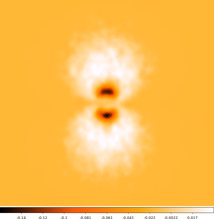
As mentioned in Section 3.1 the model used along this work is that of a bright point like source with anisotropic emission (Stalevski et al, 2016), where the emission is defined by Eq. 17, following Netzer (1987). Looking at the map of latent feature Z8 (Fig. 2(c)) the geometric signature of the model is clearly identifiable.

Appendix D Emulation Flowcharts

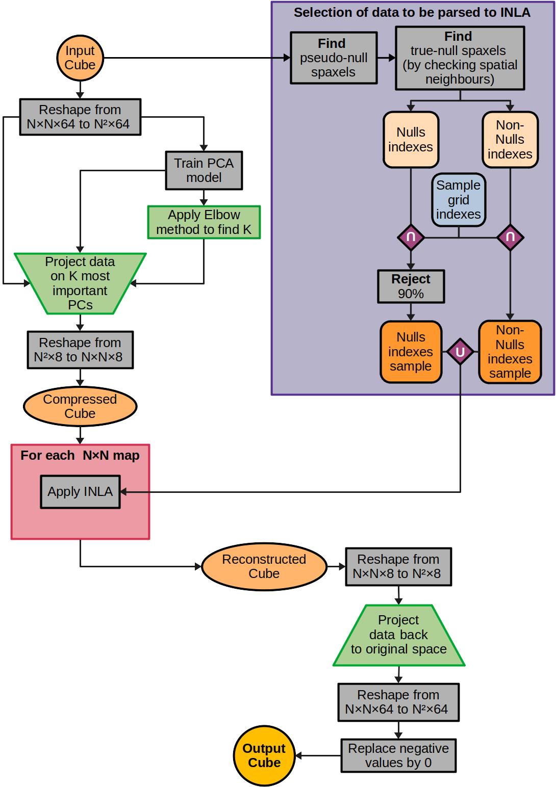
This section presents flowcharts for different emulation pipelines used in this work. In these, circles and ellipses represent data cubes at different stages of the pipeline and round cornered squares present lists of indexes. Grey rectangle boxes are operations using the data, purple diamond boxes indicate set operations ($\cap$ for intersection and $\cup$ for union) on indexes, green boxes indicate operations related to dimensionality transformation models. $\blacklozenge$ refers to the de-normalization procedure mentioned in Section 3.1.1 and $\dagger$ refers to operations described in Section 3.3.

Figure 1: Flowchart for EmulART.

Figure 2: Flowchart for the emulation pipeline that employs the PCA model with the number of components, K, determined by the elbow method. For the emulation pipeline that employs the PCA model with a number of components equal to the number of latent features of the DVAE model in EmulART (K = 8) the Elbow method block is skipped.

Appendix E Result Analysis

This section presents a detailed view of the results obtained with both AESet and EVASet. As mentioned in Section 4, for every $\tau_{9.7}$ and $\phi$ case the realization with $N_{p}=10^{8}$ was considered as the HPN reference, or “ground truth”. The remaining LPN realizations and the emulations obtained from those were compared to the HPN reference in regards to their spectral and spatial features.

For the spectral analysis we computed the normalized residuals (Eq. 18) of the spatially integrated SEDs, compared the shape of those SEDs and inspected the spatial maps of the DVAE compressed features looking for distributions compatible with the physical properties of the HPN reference.

For the spatial analysis we computed the normalized residuals and measured statistical descriptors - median and mean absolute deviation (MAD) - for each wavelength bin spatial map, for both LPN inputs and resulting emulations. To measure the impact of INLA on the reconstruction of input spaxels we count how many full, partial and null spaxels are present in the HPN reference, LPN input and the resulting emulations, and compute the TIR of each.

E.1 AESet Predictions

E.1.1 Spectral Predictions

In this section we discuss how well the spectral information is preserved, after the LPN inputs of AESet are processed by EmulART, by looking into the emulations spatially integrated SEDs.

From both Fig. 7 and Tab. 2 we determine the $N_{p}=10^{6}$ realization, with spaxel sampling of 4%, to be the most favorable input for our pipeline. This simulation is the result of 100$\times$ less photons simulated than the reference, and with the corresponding emulation using as input 4% of its spaxels which results in 2500$\times$ less input information than the present in the HPN reference. This emulation presents median residuals of $\sim$85% between 1 and 4$\mu$m, $\sim$33% between 4$\mu$m and 1mm and $\sim$42% over the whole spectral range, and 2.8% when considering the SED that results from the spatial integration of each wavelength map (less than 2% worse than the realization which was used as input). It also reconstructs over 71,000 spaxels presenting almost two times the amount of full spaxels of the reference. Appendix F shows how the pipeline goes even further with the emulated individual spaxels presenting smoother profiles than the references.

E.1.2 Spatial Predictions

This section looks at the reconstructions of sparse samples of pixels from latent feature maps and the spatial distributions that result after returning those to the original spectral space.

The impact of INLAs spatial reconstruction is evidenced by the emulations residuals having lower median values than all realizations but the reference, and mean deviations of the same order of magnitude. In the case of the emulations performed using the $N_{p}=10^{7}$ realizations as input that is even clearer, with median of the spatial residuals at wavelengths greater than 5 $\mu$m going below 30%. Furthermore, as Fig. 1 shows, there are two transitions in quality evidenced by the gaps between the median residuals. It is also shown that all lower photon count simulations have their residuals dominated by lack of information (the reader is reminded that a 100% normalized residual means that pixel holds no information), and that the spatial inference at lower wavelengths results in large over-estimations. The absence of information which heavily influences the statistical descriptors of the simulations residuals is thus curbed. This is confirmed when comparing the TIR values, where we can see that the emulation based on the lowest $N_{p}$ realizations has a TIR of 98.3% compared to the reference realization (see Tab. 2), while the $N_{p}=10^{7}$ realization’s is 65.2% (see Tab. 1).

Figure 1: Median of the normalized residuals, at each wavelengths spatial map, for every emulation obtained with $N_{p}=10^{4}$ (red), $N_{p}=10^{5}$ (green), $N_{p}=10^{6}$ (blue) and $N_{p}=10^{7}$ (cyan) realizations, for the case of a dust shell with $\tau_{9.7}=0.05$ and $\phi=0^{\circ}$. Emulations whose spatial inference was performed using as input 25% of data are represented by ($\triangle$), 11% by (+) and 4% by ($\times$). The interrupted black line marks the same metric for the LPN realizations.

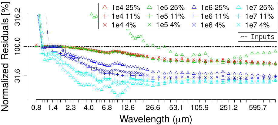
Fig. 2 shows the spatial distribution of the emulations residuals at some wavelengths, it is clear that:

• The residuals are correlated with the distance towards the center of the object, with the highest residuals populating the outer edge and the lowest in the center.

• Shorter wavelengths display higher residuals.

(a) 0.84 $\mu$m

(b) 1.85 $\mu$m

(c) 9.28 $\mu$m

(d) 211.35 $\mu$m

Figure 2: Spatial distribution of residuals, as defined in Eq. 18, for the emulation produced using as input a 4% sample of the $N_{p}=10^{6}$ realization, for the case of a dust shell with $\tau_{9.7}=0.05$ and $\phi=0^{\circ}$, at wavelengths 0.84 $\mu$m (Fig. 2(a)), 1.85 $\mu$m (Fig. 2(b)), 9.28 $\mu$m (Fig. 2(c)) and 211.35 $\mu$m (Fig. 2(d)).

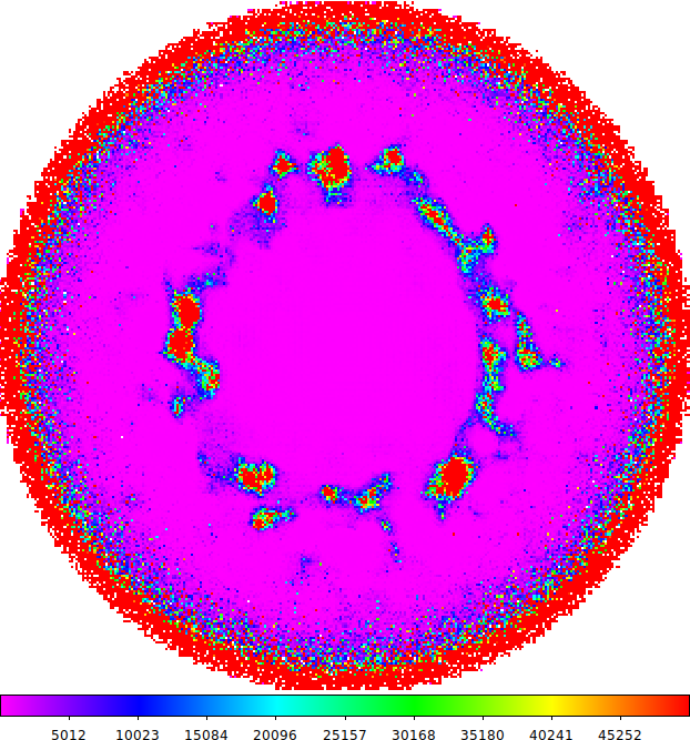
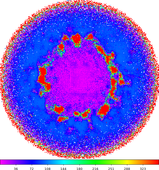
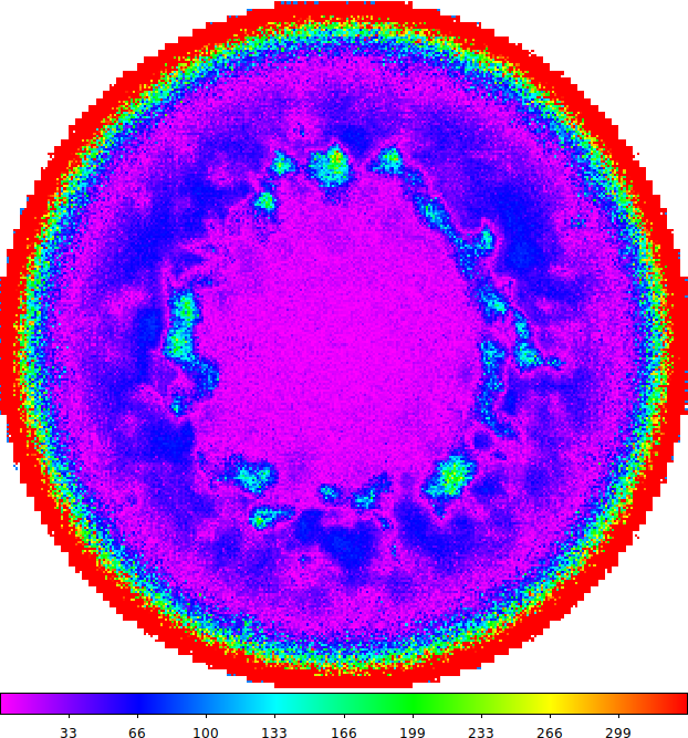
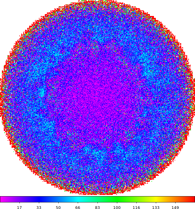
The above results were expected given that: we performed a uniform spatial sampling of an object central to a spherically symmetric dust distribution; more spatial information is available at the center of the simulated object than in the outskirts; and, at shorter wavelengths there is overall less information, as seen in the previous section, from which to build the spatial reconstruction.

It is harder to assess how accurate INLAs inference of the outskirt regions is. Those regions, given the spatial distribution of the simulated model, tend to be less dense. Nevertheless, at most wavelengths and most of the spacial distribution of the object, the residuals place the emulated value at the same order of magnitude as the reference values. Moreover, it is in these regions that INLA recovers more information, filling in the gaps.

E.2 EVASet Predictions

E.2.1 Spectral Predictions

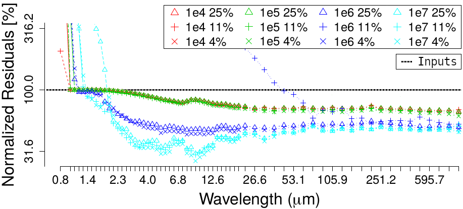
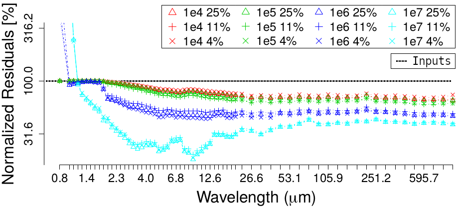
In this section we discuss how well the spectral information is preserved, after the LPN inputs of EVASet, with $\tau_{9.7}\neq 0.05$, are processed by EmulART, by once again looking into the emulations spatially integrated SEDs.

Regarding the case with $\tau_{9.7}=0.1$, Fig. 3 and Tab. 1 show that, for both tilt angles, while the shape of the emulations integrated spectra still follows closely that of the references, the residuals are now over 2$\times$ higher than with $\tau_{9.7}=0.05$. The results for the cases with $\tau_{9.7}=1.0$ confirm this trend in degrading quality of the pipeline’s spectral predictions. As seen in Fig. 11, the emulation integrated spectrum completely misses the shape of the reference spectrum, keeping the shape displayed for the cases with $\tau_{9.7}=0.05$ and $\tau_{9.7}=0.1$, a sign of over-fitting which is confirmed when inspecting individual spaxels (see Appendix F). It also underestimates the flux density and overestimates the relative magnitude of the two emission bumps in the 8 $\mu$m to 20 $\mu$m range. The median residual of the total flux density per wavelength, displayed in Tab. 1, further confirms the poor quality of the spectral predictions.

(a) $\phi=90^{\circ}$

(b) $\phi=0^{\circ}$

Figure 3: Emulations integrated SEDs, resulting from spatial inference using 25% of spatial information, and the respective normalized residuals, for the cases of dust shells with $\tau_{9.7}=0.1$, $\phi=90^{\circ}$ (Fig. 3(a)) and $\phi=0^{\circ}$ (Fig. 3(b)). The HPN reference is represented in black ($\circ$), the emulation based on the $N_{p}=10^{4}$ realization is in red ($\triangle$), on the $N_{p}=10^{5}$ in green (+), on the $N_{p}=10^{6}$ in blue ($\times$) and on the $N_{p}=10^{7}$ in cyan ($\diamond$) .

Case		LPN Input Sample	Residuals of Integrated Emul. (%)		Normalized Residuals of Emul. (%)
$\tau_{9.7}$	$\phi$ (deg)
			M	MAD	M	MAD
0.1	0	$10^{6}$ 11%	279	256	561	805
		$10^{6}$ 25%	37	10	56	32
		$10^{7}$ 11%	33.2	5.9	46	31
		$10^{7}$ 25%	32.6	5.3	48	35
	90	$10^{6}$ 11%	33	12	58	35
		$10^{6}$ 25%	30	13	54	34
		$10^{7}$ 11%	15	10	36	29
		$10^{7}$ 25%	14.1	9.9	35	28
1.0	0	$10^{6}$ 11%	89.8	5.2	92.1	9.8
		$10^{6}$ 25%	89.8	5.3	92	10
		$10^{7}$ 11%	91	2e+9	93.5	9.4
		$10^{7}$ 25%	91	7e+5	94.1	7.8
	90	$10^{6}$ 11%	89.6	7.8	92.3	8.1
		$10^{6}$ 25%	90.6	5.8	92.6	7.7
		$10^{7}$ 11%	91	4e+8	93.0	9.1
		$10^{7}$ 25%	91	3e+7	93.5	8.1

Table 1: Comparison of statistics for the residuals of the spatial integration SEDs (columns 4 and 5) and of the residuals overall wavelengths (columns 6 and 7), for the emulations that took as input LPN realizations of dust shells with $\tau_{9.7}\in\{0.1,1.0\}$, $\phi\in\{0^{\circ},90^{\circ}\}$, and $N_{p}\in\{10^{6},10^{7}\}$.

E.2.2 Spatial Predictions

Regarding spatial information, for emulations with LPN inputs of $\tau_{9.7}=0.05$ and $\phi=90^{\circ}$ we observe the same behavior in the performance metrics as with the $\phi=0^{\circ}$ case. Tab. 2 shows that the overall median residuals decrease with the increase of $N_{p}$. The median residuals per wavelength, displayed in Fig. 4, present a similar behavior to those of the $\phi=0^{\circ}$ case.

LPN Input Sample	Total Emul. Time (min)	Normalized Residuals of Emul. (%)		Information of Emulation
		M	MAD	TIR (%)	Null Spxs ($N$)	Empty Spxs ($\Delta N$)	Full Spxs ($N$)	Partial Spxs ($N$)
$10^{4}$ 4%	7.2	74	36	98.1	20,497	2,641	69,503	0
$10^{4}$ 11%	22.2	74	36
$10^{4}$ 25%	16.3	75	36
$10^{5}$ 4%	6.2	73	36	101.6	18,002	146	71,998	0
$10^{5}$ 11%	21.7	70	40
$10^{5}$ 25%	13.4	67	44
$10^{6}$ 4%	7.2	47	43	103.2	16,872	-984	73,128	0
$10^{6}$ 11%	22.7	48	47
$10^{6}$ 25%	15.9	42	40
$10^{7}$ 4%	8.0	36	38	103.2	16,833	-1,023	73,167	0
$10^{7}$ 11%	19.1	36	39
$10^{7}$ 25%	15.2	32	34

Table 2: Statistics regarding how the different emulations, of the case of a dust shell with $\tau_{9.7}=0.05$ and $\phi=90^{\circ}$, compared to the HPN reference. The results are similar to those displayed in Tab. 3.

Figure 4: Median of the normalized residuals, at each wavelengths spatial map, for every emulation obtained with $N_{p}=10^{4}$ (red), $N_{p}=10^{5}$ (green), $N_{p}=10^{6}$ (blue) and $N_{p}=10^{7}$ (cyan) realizations, for the case of a dust shell with $\tau_{9.7}=0.05$ and $\phi=90^{\circ}$. Emulations whose spatial inference was performed taking as input 25% of the data are represented by ($\triangle$), 11% by (+) and 4% by ($\times$). The interrupted black line marks the same metric for the realizations used as input.

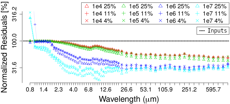
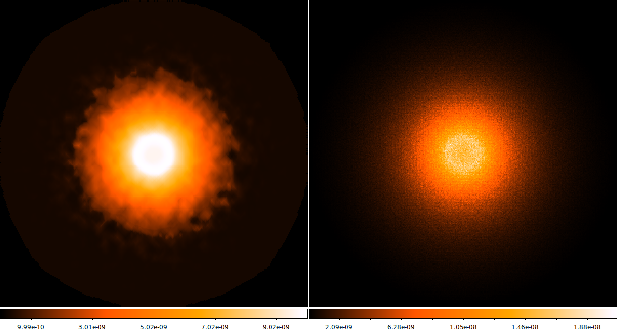
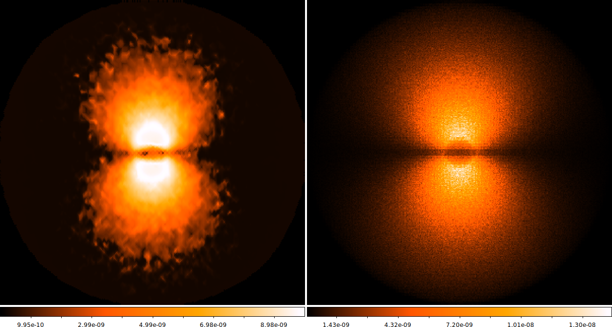
Fig. 5 shows that the emulation of models with excessive emission within the central regions in comparison to the reference, while in Fig. 6 the prediction for the peripheral region is more isotropic than the reference, this is even clearer when consulting the spatial distribution of residuals for these emulations in Fig. 7.

(a) 0.84 $\mu$m

(b) 1.85 $\mu$m

Figure 5: Emulation produced using as input a 4% sample of the $N_{p}=10^{6}$ realization, left, and HPN reference, right, for the case of a dust shell with $\tau_{9.7}=0.05$ and $\phi=90^{\circ}$, at wavelengths 0.84 $\mu$m (Fig. 5(a)) and 1.85 $\mu$m (Fig. 5(b)).

(a) 9.28 $\mu$m

(b) 211.35 $\mu$m

Figure 6: Emulation produced using as input a 4% sample of the $N_{p}=10^{6}$ realization, left, and HPN reference, right, for the case of a dust shell with $\tau_{9.7}=0.05$ and $\phi=90^{\circ}$, at wavelengths 9.28 $\mu$m (Fig. 6(a)) and 211.35 $\mu$m (Fig. 6(b)).

(a) 0.84 $\mu$m

(b) 1.85 $\mu$m

(c) 9.28 $\mu$m

(d) 211.35 $\mu$m

Figure 7: Spatial distribution of residuals, as defined in Eq. 18, for the emulation produced using as input a 4% sample of the $N_{p}=10^{6}$ realization, for the case of a dust shell with $\tau_{9.7}=0.05$ and $\phi=90^{\circ}$, at wavelengths 0.84 $\mu$m (Fig. 7(a)), 1.85 $\mu$m (Fig. 7(b)), 9.28 $\mu$m (Fig. 7(c)) and 211.35 $\mu$m (Fig. 7(d)).

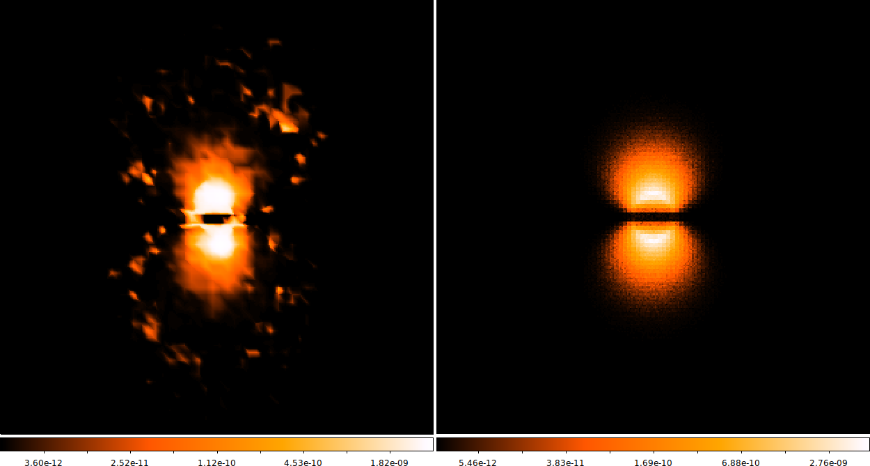
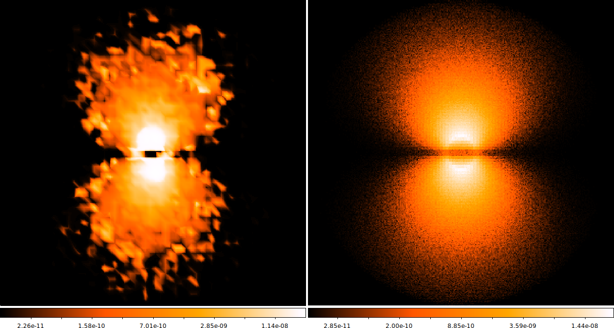
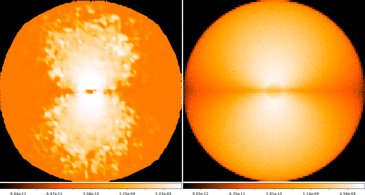
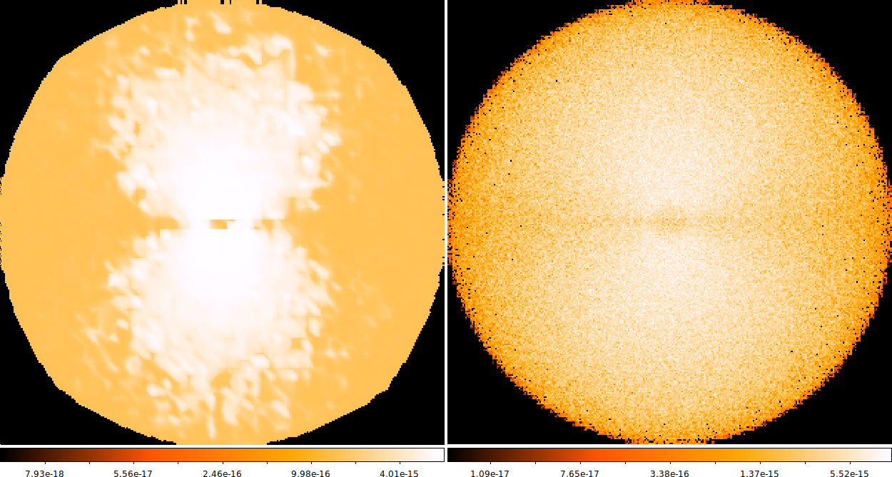
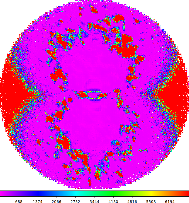
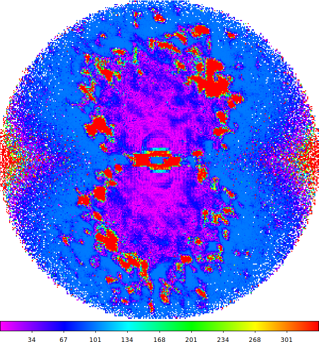
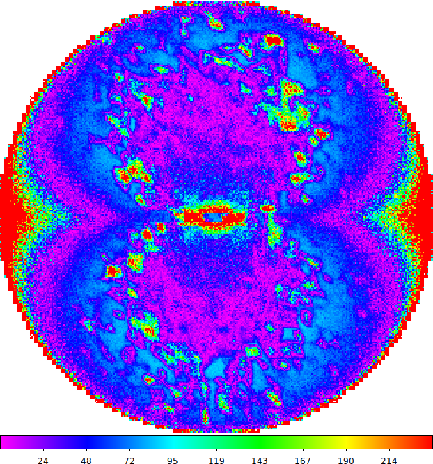
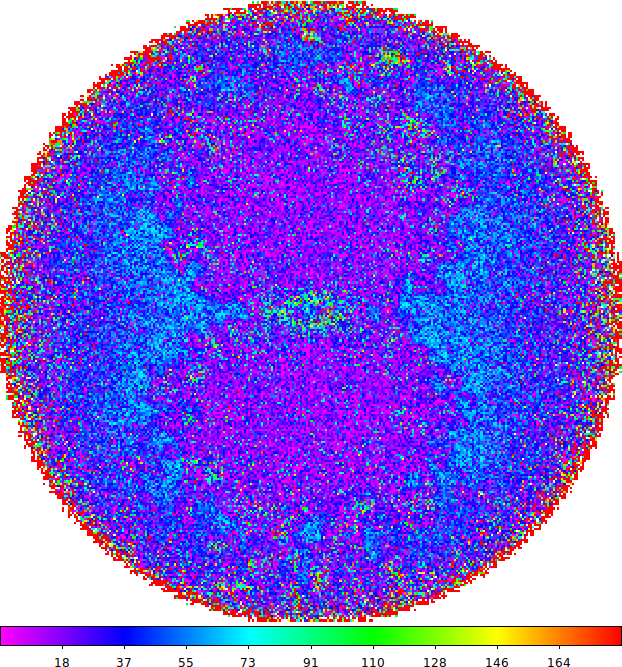
As with the $\tau_{9.7}=1.0$ cases, for both tilt angle cases of $\tau_{9.7}=0.1$ we observe a similar trend in the overall residuals. Fig. 9 shows that while the overall morphology of the spatial distribution is well recovered, the flux density value range for the emulations is underestimated, though not as considerably as with the $\tau_{9.7}=1.0$ cases, and the contrast between the central and peripheral regions is higher than in the HPN references. This indicates a bias within the pipeline. Appendix F further details into the likely source of such bias by comparing individual spaxels of emulations and HPN simulations.

(a) $\phi=0^{\circ}$

(b) $\phi=90^{\circ}$

Figure 8: Median of the normalized residuals, at each wavelengths spatial map, for every emulation obtained with $N_{p}=10^{4}$ (red), $N_{p}=10^{5}$ (green), $N_{p}=10^{6}$ (blue) and $N_{p}=10^{7}$ (cyan) realizations, for the case of a dust shell with $\tau_{9.7}=0.1$, with $\phi=0^{\circ}$ (Fig. 8(a)) and $\phi=90^{\circ}$ (Fig. 8(b)). Emulations whose spatial inference was performed using 25% of data are represented by ($\triangle$), 11% by (+) and 4% by ($\times$). The interrupted black line marks the same metric for the LPN inputs.

(a) $\phi=0^{\circ}$

(b) $\phi=90^{\circ}$

Figure 9: Emulation produced using as input a 25% sample of the $N_{p}=10^{6}$ realization, left, and HPN reference, right, for the case of dust shells with $\tau_{9.7}=0.1$, at wavelengths 9.28 $\mu$m, with $\phi=0^{\circ}$, (Fig. 9(a)) and $\phi=90^{\circ}$ (Fig. 9(b)).

Appendix F Single Spaxels

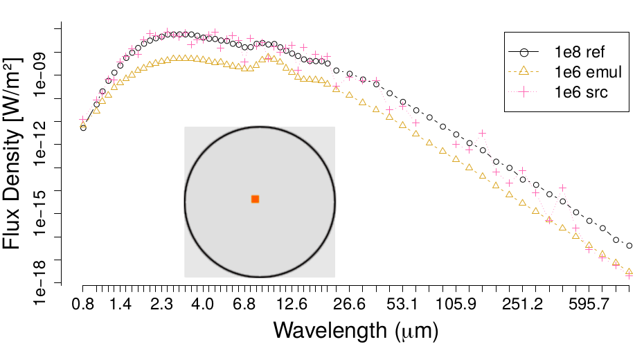
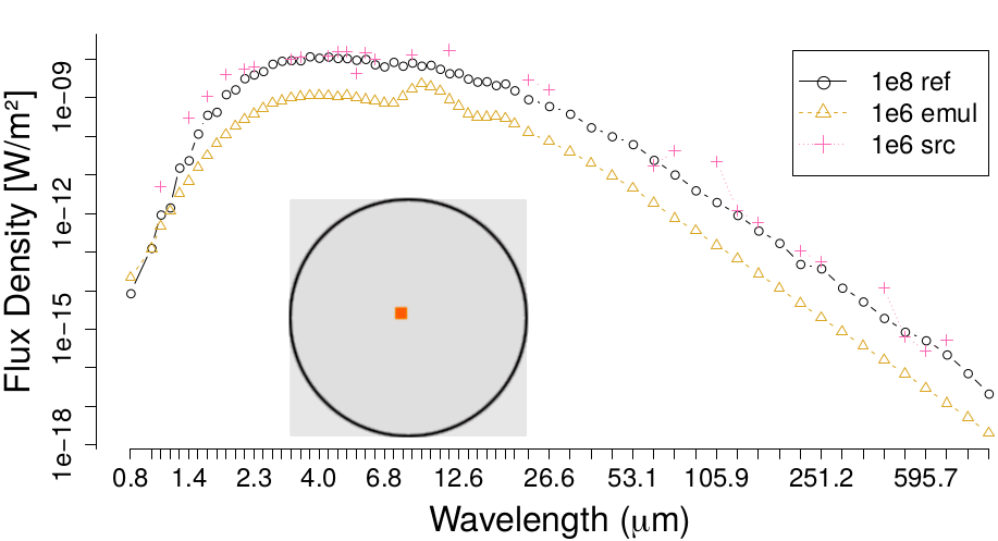
Figs. 1, 2 and 3 compare 3 different spaxels between their versions in the LPN input, HPN reference and emulation based on the LPN input. These spaxels are radially aligned: one at the center of the object, another on the outskirts and another in-between those two. The emulations where achieved using 25% of the corresponding source cube spaxels.

Some things easily noticeable are the underestimation of the shorter wavelengths for the versions of these spaxels taken from emulations based on $N_{p}=10^{4}$ and $N_{p}=10^{5}$ realizations. Nevertheless in those cases the LPN input spaxel is not complete, i.e. there are zero values at some wavelengths, if not all, meaning the pipeline is reaching what it was designed to do: take a sparse compressed model, infer the missing information and then decompress it.

(a) $N_{p}=10^{4}$

(b) $N_{p}=10^{5}$

(c) $N_{p}=10^{6}$

(d) $N_{p}=10^{7}$

Figure 1: Comparison of some emulations spaxels located in row = 150, col = 150, against the HPN references and the LPN input (indicated in each plot), for the case of a dust shell with $\tau_{9.7}=0.05$ and $\phi=0^{\circ}$. The emulations were performed using 25% of the LPN input spatial information. HPN references spaxel in black ($\circ$), emulations in gold ($\triangle$) and LPN inputs, upon which the emulation was performed, in pink (+).

(a) $N_{p}=10^{4}$

(b) $N_{p}=10^{5}$

(c) $N_{p}=10^{6}$

(d) $N_{p}=10^{7}$

Figure 2: Comparison of some emulations spaxels located in row = 150, col = 210, against the HPN references and the LPN input (indicated in each plot), for the case of a dust shell with $\tau_{9.7}=0.05$ and $\phi=0^{\circ}$. The emulations were performed using 25% of the LPN input spatial information. HPN references spaxel in black ($\circ$), emulations in gold ($\triangle$) and LPN inputs, upon which the emulation was performed, in pink (+).

(a) $N_{p}=10^{4}$

(b) $N_{p}=10^{5}$

(c) $N_{p}=10^{6}$

(d) $N_{p}=10^{7}$

Figure 3: Comparison of some emulations spaxels located in row = 150, col = 270, against the HPN references and the LPN input (indicated in each plot), for the case of a dust shell with $\tau_{9.7}=0.05$ and $\phi=0^{\circ}$. The emulations were performed using 25% of the LPN input spatial information. HPN references spaxel in black ($\circ$), emulations in gold ($\triangle$) and LPN inputs, upon which the emulation was performed, in pink (+).

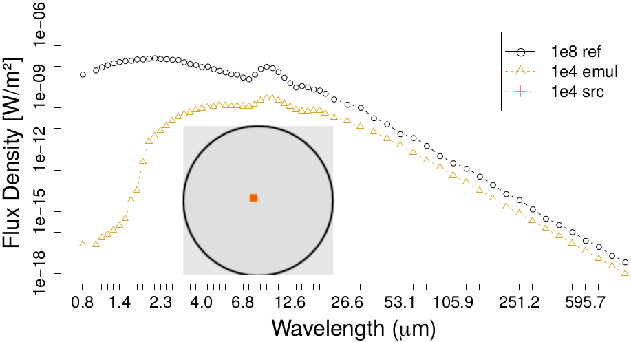
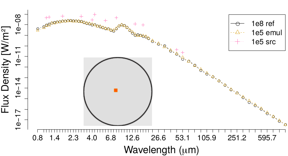
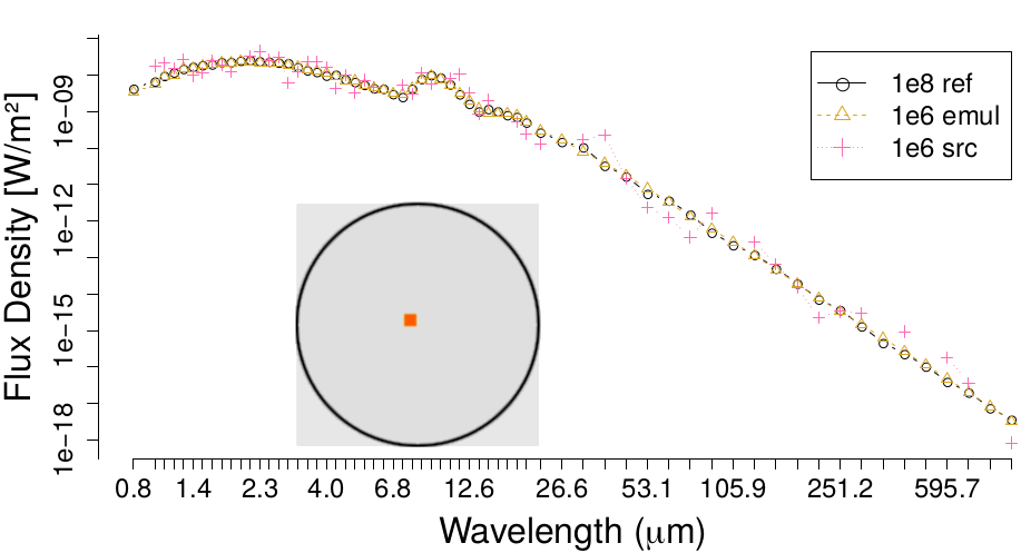
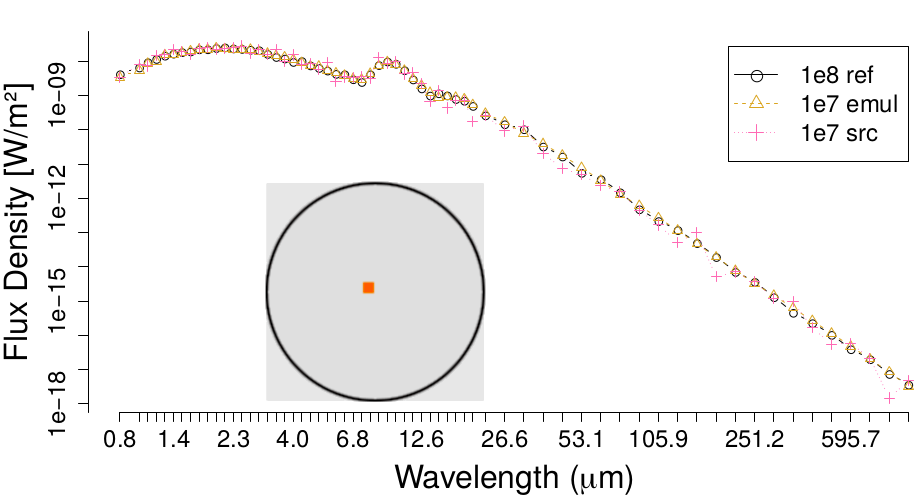
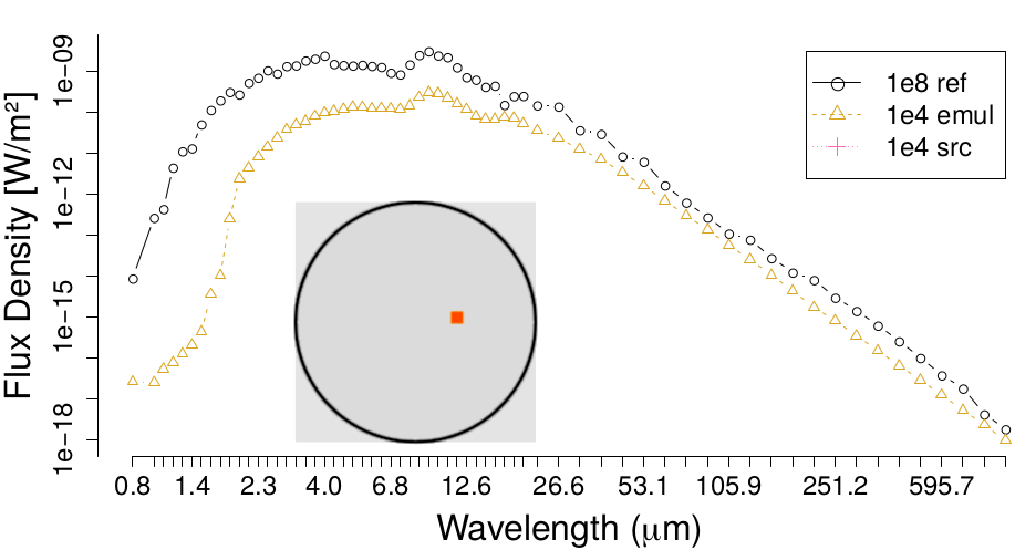
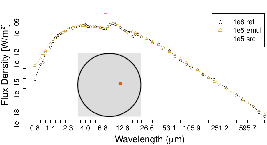
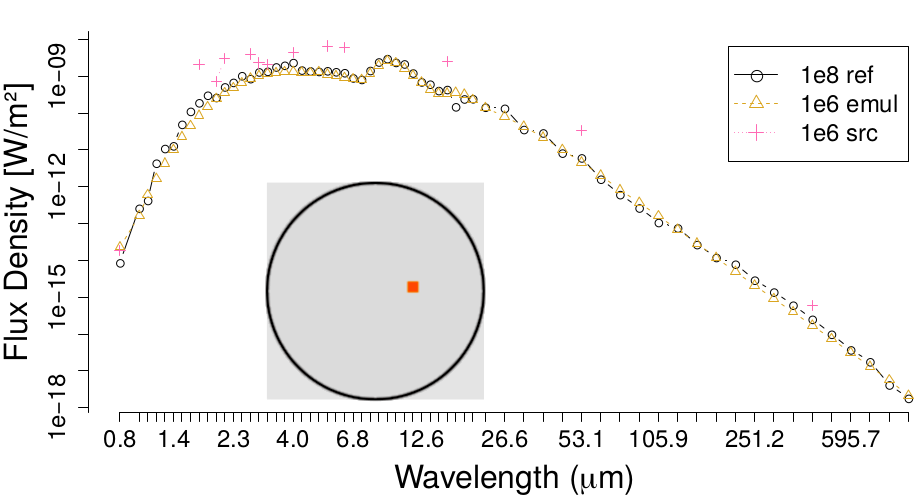
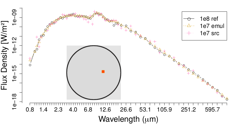
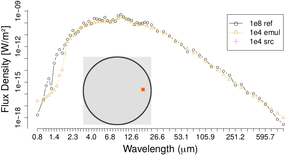
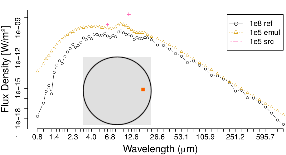
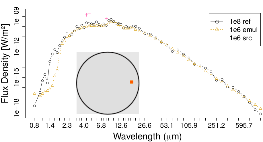
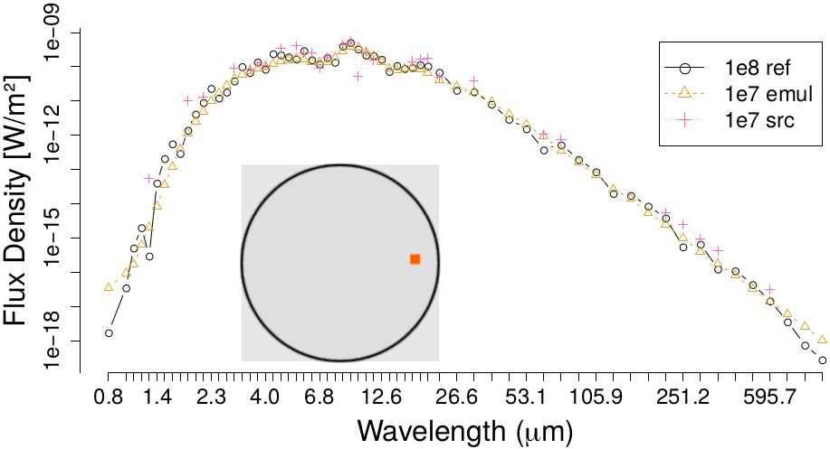
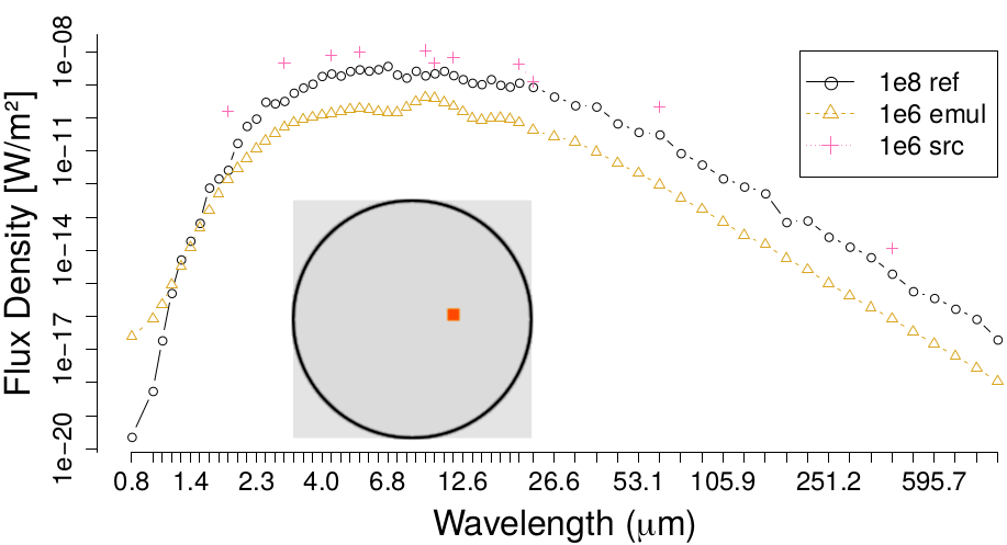
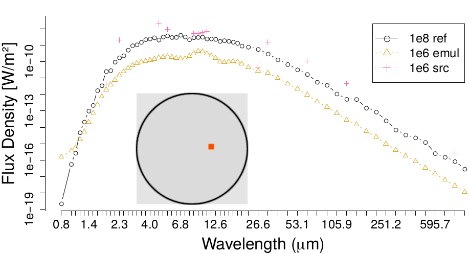
Figs. 4, 5 and 6 compare 3 different spaxels from the same spatial locations as before. The emulations were achieved using 11% of the corresponding LPN input cube spaxels, which are the $\tau_{9.7}=1.0$ and $\phi\in\{0^{\circ},90^{\circ}\}$ cases. Since the simulated bright central source has anisotropic emission at greater optical depths, $\tau_{9.7}$, we can expect that for different viewing angles, $\phi$, the shapes of spaxels near the central region of the spatial distribution will present differences as can be seen in the reference curves of Fig. 4.

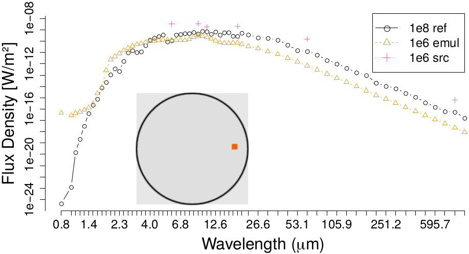
For both the face-on and edge-on cases, at all displayed positions, we can make the same assessment, that the shape of the emulated spaxels does not follow the shape of the HPN references. As the simulated models dust density increases so does the likelihood of scattering and absorption of light by the medium, consequently the peak emission features are flattened into the continuum. Figs. 4 and 5 show that the emulation of the spaxels in those regions is one to two orders of magnitude too low while the relative flux between the emission peak, at 9.7 $\mu$m, and the continuum is over-estimated, the allocation of flux along the spaxels does not match that of the reference. For the outer spaxels, 6, the flux mismatch is greater for longer wavelengths but still the emulation spaxels present a peak emission feature while the references no longer show it. This is a clear sign that the DVAE model is biased.

(a) $\phi=0^{\circ}$

(b) $\phi=90^{\circ}$

Figure 4: Comparison of emulations spaxels, located in row = 150, col = 150, against the HPN references and the $N_{p}=10^{6}$ realization, for the case of a dust shell with $\tau_{9.7}=1.0$, with $\phi=0^{\circ}$ (Fig. 4(a)) and $\phi=90^{\circ}$ (Fig. 4(b)). HPN references spaxel in black ($\circ$), emulations in gold ($\triangle$) and LPN inputs, upon which the emulation was performed, in pink (+).

(a) $\phi=0^{\circ}$

(b) $\phi=90^{\circ}$

Figure 5: Comparison of emulations spaxels, located in row = 150, col = 210, against the HPN references and the $N_{p}=10^{6}$ realization, for the cases of dust shells with $\tau_{9.7}=1.0$, with $\phi=0^{\circ}$ (Fig. 4(a)) and $\phi=90^{\circ}$ (Fig. 4(b)). HPN references spaxel in black ($\circ$), emulations in gold ($\triangle$) and LPN inputs, upon which the emulation was performed, in pink (+).

(a) $\phi=0^{\circ}$

(b) $\phi=90^{\circ}$

Figure 6: Comparison of emulations spaxels, located in row = 150, col = 270, against the HPN references and the $N_{p}=10^{6}$ realization, for the cases of dust shells with $\tau_{9.7}=1.0$, with $\phi=0^{\circ}$ (Fig. 4(a)) and $\phi=90^{\circ}$ (Fig. 4(b)). HPN references spaxel in black ($\circ$), emulations in gold ($\triangle$) and LPN inputs, upon which the emulation was performed, in pink (+).

References

- \bibcommenthead
- Allaire and Chollet (2021) Allaire J, Chollet F (2021) keras: R Interface to ’Keras’. URL https://CRAN.R-project.org/package=keras, r package version 2.6.1
- André et al (2010) André P, Men’shchikov A, Bontemps S, et al (2010) From filamentary clouds to prestellar cores to the stellar IMF: Initial highlights from the Herschel Gould Belt Survey. Astronomy and Astrophysics 518:L102. 10.1051/0004-6361/201014666, https://arxiv.org/abs/arXiv:1005.2618 [astro-ph.GA]
- Babusiaux et al (2020) Babusiaux C, Fourtune-Ravard C, Hottier C, et al (2020) FEDReD. I. 3D extinction and stellar maps by Bayesian deconvolution. Astronomy and Astrophysics 641:A78. 10.1051/0004-6361/202037466, https://arxiv.org/abs/arXiv:2007.04455 [astro-ph.GA]
- Bachl et al (2019) Bachl FE, Lindgren F, Borchers DL, et al (2019) inlabru: an r package for bayesian spatial modelling from ecological survey data. Methods in Ecology and Evolution 10(6):760–766. https://doi.org/10.1111/2041-210X.13168, URL https://besjournals.onlinelibrary.wiley.com/doi/abs/10.1111/2041-210X.13168, https://arxiv.org/abs/https://besjournals.onlinelibrary.wiley.com/doi/pdf/10.1111/2041-210X.13168
- Baes et al (2011) Baes M, Verstappen J, De Looze I, et al (2011) Efficient Three-dimensional NLTE Dust Radiative Transfer with SKIRT. The Astrophysical Journals 196(2):22. 10.1088/0067-0049/196/2/22, https://arxiv.org/abs/arXiv:1108.5056 [astro-ph.CO]
- Beech (1987) Beech M (1987) Are lynds dark clouds fractals? Astrophysics and Space Science 133(1):193–195. 10.1007/BF00637432
- Betoule et al (2014) Betoule M, Kessler R, Guy J, et al (2014) Improved cosmological constraints from a joint analysis of the SDSS-II and SNLS supernova samples. Astronomy and Astrophysics 568:A22. 10.1051/0004-6361/201423413, https://arxiv.org/abs/arXiv:1401.4064 [astro-ph.CO]
- Boulais et al (2021) Boulais A, Berné O, Faury G, et al (2021) Unmixing methods based on nonnegativity and weakly mixed pixels for astronomical hyperspectral datasets. Astronomy and Astrophysics 647:A105. 10.1051/0004-6361/201936399, https://arxiv.org/abs/arXiv:2011.09742 [astro-ph.IM]
- Camps and Baes (2015) Camps P, Baes M (2015) SKIRT: An advanced dust radiative transfer code with a user-friendly architecture. Astronomy and Computing 9:20–33. 10.1016/j.ascom.2014.10.004, https://arxiv.org/abs/arXiv:1410.1629 [astro-ph.IM]
- Camps and Baes (2020) Camps P, Baes M (2020) SKIRT 9: Redesigning an advanced dust radiative transfer code to allow kinematics, line transfer and polarization by aligned dust grains. Astronomy and Computing 31:100381. 10.1016/j.ascom.2020.100381, https://arxiv.org/abs/arXiv:2003.00721 [astro-ph.GA]
- Collins et al (1974) Collins JD, Hart GC, Haselman TK, et al (1974) Statistical Identification of Structures. AIAA Journal 12(2):185–190. 10.2514/3.49190
- Cox et al (2012) Cox NLJ, Kerschbaum F, van Marle AJ, et al (2012) A far-infrared survey of bow shocks and detached shells around AGB stars and red supergiants. Astronomy and Astrophysics 537:A35. 10.1051/0004-6361/201117910, https://arxiv.org/abs/arXiv:1110.5486 [astro-ph.GA]
- De Looze et al (2014) De Looze I, Fritz J, Baes M, et al (2014) High-resolution, 3D radiative transfer modeling. I. The grand-design spiral galaxy M 51. Astronomy and Astrophysics 571:A69. 10.1051/0004-6361/201424747, https://arxiv.org/abs/arXiv:1409.3857 [astro-ph.GA]
- Doersch (2016) Doersch C (2016) Tutorial on Variational Autoencoders. arXiv e-prints arXiv:1606.05908. https://arxiv.org/abs/arXiv:1606.05908 [stat.ML]
- Dunne et al (2011) Dunne L, Gomez HL, da Cunha E, et al (2011) Herschel-ATLAS: rapid evolution of dust in galaxies over the last 5 billion years. Monthly Notices of the Royal Astronomical Society 417(2):1510–1533. 10.1111/j.1365-2966.2011.19363.x, https://arxiv.org/abs/arXiv:1012.5186 [astro-ph.CO]
- Falgarone et al (1991) Falgarone E, Phillips TG, Walker CK (1991) The Edges of Molecular Clouds: Fractal Boundaries and Density Structure. The Astrophysical Journal 378:186. 10.1086/170419
- Fritz et al (2012) Fritz J, Gentile G, Smith MWL, et al (2012) The Herschel Exploitation of Local Galaxy Andromeda (HELGA). I. Global far-infrared and sub-mm morphology. Astronomy and Astrophysics 546:A34. 10.1051/0004-6361/201118619, https://arxiv.org/abs/arXiv:1112.3348 [astro-ph.CO]
- González-Gaitán et al (2019) González-Gaitán S, de Souza RS, Krone-Martins A, et al (2019) Spatial field reconstruction with INLA: application to IFU galaxy data. Monthly Notices of the Royal Astronomical Society 482(3):3880–3891. 10.1093/mnras/sty2881, https://arxiv.org/abs/arXiv:1802.06280 [astro-ph.IM]
- Guo et al (2019) Guo H, Zhuang X, Rabczuk T (2019) A deep collocation method for the bending analysis of kirchhoff plate. Computers, Materials & Continua 59(2):433–456. 10.32604/cmc.2019.06660, URL http://www.techscience.com/cmc/v59n2/27944
- Gómez-Rubio (2021) Gómez-Rubio V (2021) Bayesian Inference with INLA. Chapman & Hall/CRC Press,Boca Raton, FL.
- Haas et al (2000) Haas M, Müller SAH, Chini R, et al (2000) Dust in PG quasars as seen by ISO. Astronomy and Astrophysics 354:453–466
- Hinton and Salakhutdinov (2006) Hinton G, Salakhutdinov R (2006) Reducing the dimensionality of data with neural networks. Science 313:504–507. 10.1126/science.1127647
- Hinton and van Camp (1993) Hinton GE, van Camp D (1993) Keeping the neural networks simple by minimizing the description length of the weights. In: Proceedings of the Sixth Annual Conference on Computational Learning Theory. Association for Computing Machinery, New York, NY, USA, COLT ’93, p 5–13, 10.1145/168304.168306, URL https://doi.org/10.1145/168304.168306
- Ichinohe and Yamada (2019) Ichinohe Y, Yamada S (2019) Neural network-based anomaly detection for high-resolution X-ray spectroscopy. Monthly Notices of the Royal Astronomical Society 487(2):2874–2880. 10.1093/mnras/stz1528, https://arxiv.org/abs/arXiv:1905.13434 [astro-ph.IM]
- Ishida and de Souza (2011) Ishida EEO, de Souza RS (2011) Hubble parameter reconstruction from a principal component analysis: minimizing the bias. Astronomy and Astrophysics 527:A49. 10.1051/0004-6361/201015281, https://arxiv.org/abs/arXiv:1012.5335 [astro-ph.CO]
- Ishida et al (2011) Ishida EEO, de Souza RS, Ferrara A (2011) Probing cosmic star formation up to z= 9.4 with gamma-ray bursts. Monthly Notices of the Royal Astronomical Society 418(1):500–504. 10.1111/j.1365-2966.2011.19501.x, https://arxiv.org/abs/arXiv:1106.1745 [astro-ph.CO]
- Jia et al (2020) Jia P, Li X, Li Z, et al (2020) Point spread function modelling for wide-field small-aperture telescopes with a denoising autoencoder. Monthly Notices of the Royal Astronomical Society 493(1):651–660. 10.1093/mnras/staa319, https://arxiv.org/abs/arXiv:2001.11716 [astro-ph.IM]
- Jiwoong Im et al (2015) Jiwoong Im D, Ahn S, Memisevic R, et al (2015) Denoising Criterion for Variational Auto-Encoding Framework. arXiv e-prints arXiv:1511.06406. https://arxiv.org/abs/arXiv:1511.06406 [cs.LG]
- Jolliffe and Cadima (2016) Jolliffe IT, Cadima J (2016) Principal component analysis: a review and recent developments. Philosophical Transactions of the Royal Society of London Series A 374(2065):20150,202. 10.1098/rsta.2015.0202
- Klambauer et al (2017) Klambauer G, Unterthiner T, Mayr A, et al (2017) Self-Normalizing Neural Networks. arXiv e-prints arXiv:1706.02515. https://arxiv.org/abs/arXiv:1706.02515 [cs.LG]
- Kopf et al (2021) Kopf A, Fortuin V, Somnath VR, et al (2021) Mixture-of-experts variational autoencoder for clustering and generating from similarity-based representations on single cell data. PLoS computational biology 17(6). https://doi.org/10.1371/journal.pcbi.1009086
- Krone-Martins and Moitinho (2014) Krone-Martins A, Moitinho A (2014) UPMASK: unsupervised photometric membership assignment in stellar clusters. Astronomy and Astrophysics 561:A57. 10.1051/0004-6361/201321143, https://arxiv.org/abs/arXiv:1309.4471 [astro-ph.IM]
- Logan and Fotopoulou (2020) Logan CHA, Fotopoulou S (2020) Unsupervised star, galaxy, QSO classification. Application of HDBSCAN. Astronomy and Astrophysics 633:A154. 10.1051/0004-6361/201936648, https://arxiv.org/abs/arXiv:1911.05107 [astro-ph.GA]
- Mattila (1970) Mattila K (1970) Interpretation of the surface brightness of dark nebulae. Astronomy and Astrophysics 9:53
- Minka (2013) Minka TP (2013) Expectation Propagation for approximate Bayesian inference. arXiv e-prints arXiv:1301.2294. https://arxiv.org/abs/arXiv:1301.2294 [cs.AI]
- Netzer (1987) Netzer H (1987) Quasar discs. II - A composite model for the broad-line region. Monthly Notices of the Royal Astronomical Society 225:55–72. 10.1093/mnras/225.1.55
- O’Briain et al (2020) O’Briain T, Ting YS, Fabbro S, et al (2020) Interpreting Stellar Spectra with Unsupervised Domain Adaptation. arXiv e-prints arXiv:2007.03112. https://arxiv.org/abs/arXiv:2007.03112 [astro-ph.SR]
- Portillo et al (2020) Portillo SKN, Parejko JK, Vergara JR, et al (2020) Dimensionality Reduction of SDSS Spectra with Variational Autoencoders. The Astronomical Journal 160(1):45. 10.3847/1538-3881/ab9644, https://arxiv.org/abs/arXiv:2002.10464 [astro-ph.IM]
- R Core Team (2021) R Core Team (2021) R: A Language and Environment for Statistical Computing. R Foundation for Statistical Computing, Vienna, Austria, URL https://www.R-project.org/
- Ralph et al (2019) Ralph NO, Norris RP, Fang G, et al (2019) Radio Galaxy Zoo: Unsupervised Clustering of Convolutionally Auto-encoded Radio-astronomical Images. Publications of the Astronomical Society of the Pacific 131(1004):108,011. 10.1088/1538-3873/ab213d, https://arxiv.org/abs/arXiv:1906.02864 [astro-ph.IM]
- Ren et al (2018) Ren B, Pueyo L, Zhu GB, et al (2018) Non-negative Matrix Factorization: Robust Extraction of Extended Structures. The Astrophysical Journal 852(2):104. 10.3847/1538-4357/aaa1f2, https://arxiv.org/abs/arXiv:1712.10317 [astro-ph.IM]
- Rho et al (2009) Rho J, Reach WT, Tappe A, et al (2009) Spitzer Observations of the Young Core-Collapse Supernova Remnant 1E0102-72.3: Infrared Ejecta Emission and Dust Formation. The Astrophysical Journal 700(1):579–596. 10.1088/0004-637X/700/1/579
- Roark et al (1974) Roark T, Roark B, Collins IG. W. (1974) Monte Carlo Model of Reflection Nebulae: Intensity Gradients. The Astrophysical Journal 190:67–72. 10.1086/152847
- Rue et al (2009) Rue H, Martino S, Chopin N (2009) Approximate bayesian inference for latent gaussian models by using integrated nested laplace approximations. Journal of the Royal Statistical Society: Series B (Statistical Methodology) 71(2):319–392. https://doi.org/10.1111/j.1467-9868.2008.00700.x, URL https://rss.onlinelibrary.wiley.com/doi/abs/10.1111/j.1467-9868.2008.00700.x, https://arxiv.org/abs/https://rss.onlinelibrary.wiley.com/doi/pdf/10.1111/j.1467-9868.2008.00700.x
- Sasdelli et al (2014) Sasdelli M, Hillebrandt W, Aldering G, et al (2014) A metric space for Type Ia supernova spectra. Monthly Notices of the Royal Astronomical Society 447(2):1247–1266. 10.1093/mnras/stu2416, URL https://doi.org/10.1093/mnras/stu2416, https://arxiv.org/abs/https://academic.oup.com/mnras/article-pdf/447/2/1247/8093453/stu2416.pdf
- Smole et al (2022, submitted) Smole M, et al (2022, submitted) Spatial field reconstruction with INLA: Application to simulated galaxies.
- Stalevski et al (2016) Stalevski M, Ricci C, Ueda Y, et al (2016) The dust covering factor in active galactic nuclei. Monthly Notices of the Royal Astronomical Society 458(3):2288–2302. 10.1093/mnras/stw444, https://arxiv.org/abs/arXiv:1602.06954 [astro-ph.GA]
- Stalevski et al (2019) Stalevski M, Tristram KRW, Asmus D (2019) Dissecting the active galactic nucleus in Circinus - II. A thin dusty disc and a polar outflow on parsec scales. Monthly Notices of the Royal Astronomical Society 484(3):3334–3355. 10.1093/mnras/stz220, https://arxiv.org/abs/arXiv:1901.05488 [astro-ph.GA]
- Steinacker et al (2013) Steinacker J, Baes M, Gordon KD (2013) Three-Dimensional Dust Radiative Transfer*. Annual Review of Astronomy and Astrophysics 51(1):63–104. 10.1146/annurev-astro-082812-141042, https://arxiv.org/abs/arXiv:1303.4998 [astro-ph.IM]
- Tierney and Kadane (1986) Tierney L, Kadane JB (1986) Accurate approximations for posterior moments and marginal densities. Journal of the American Statistical Association 81(393):82–86. 10.1080/01621459.1986.10478240, URL https://www.tandfonline.com/doi/abs/10.1080/01621459.1986.10478240, https://arxiv.org/abs/https://www.tandfonline.com/doi/pdf/10.1080/01621459.1986.10478240
- Verstocken et al (2020) Verstocken S, Nersesian A, Baes M, et al (2020) High-resolution, 3D radiative transfer modelling. II. The early-type spiral galaxy M 81. Astronomy and Astrophysics 637:A24. 10.1051/0004-6361/201935770, https://arxiv.org/abs/arXiv:2004.03615 [astro-ph.GA]
- Viaene et al (2017) Viaene S, Baes M, Tamm A, et al (2017) The Herschel Exploitation of Local Galaxy Andromeda (HELGA). VII. A SKIRT radiative transfer model and insights on dust heating. Astronomy and Astrophysics 599:A64. 10.1051/0004-6361/201629251, https://arxiv.org/abs/arXiv:1609.08643 [astro-ph.GA]
- Wang et al (2021) Wang YC, Xie YB, Zhang TJ, et al (2021) Likelihood-free Cosmological Constraints with Artificial Neural Networks: An Application on Hubble Parameters and SNe Ia. The Astrophysical Journals 254(2):43. 10.3847/1538-4365/abf8aa, https://arxiv.org/abs/arXiv:2005.10628 [astro-ph.CO]
- Wells et al (1981) Wells DC, Greisen EW, Harten RH (1981) FITS - a Flexible Image Transport System. Astronomy and Astrophysics, Supplement 44:363
- Zhuang et al (2021) Zhuang X, Guo H, Alajlan N, et al (2021) Deep autoencoder based energy method for the bending, vibration, and buckling analysis of kirchhoff plates with transfer learning. European Journal of Mechanics - A/Solids 87:104,225. https://doi.org/10.1016/j.euromechsol.2021.104225, URL https://www.sciencedirect.com/science/article/pii/S099775382100019X
- Zhukovska et al (2008) Zhukovska S, Gail HP, Trieloff M (2008) Evolution of interstellar dust and stardust in the solar neighbourhood. Astronomy and Astrophysics 479(2):453–480. 10.1051/0004-6361:20077789, https://arxiv.org/abs/arXiv:0706.1155 [astro-ph]
- Zorich et al (2020) Zorich L, Pichara K, Protopapas P (2020) Streaming classification of variable stars. Monthly Notices of the Royal Astronomical Society 492(2):2897–2909. 10.1093/mnras/stz3426, https://arxiv.org/abs/arXiv:1912.02235 [astro-ph.IM]