Quantum optomechanics in tripartite systems

Abstract

Owing to their long-lifetimes at cryogenic temperatures, mechanical oscillators are recognized as an attractive resource for quantum information science and as a testbed for fundamental physics. Key to these applications is the ability to prepare, manipulate and measure quantum states of mechanical motion. Through an exact formal solution to the Schrodinger equation, we show how tripartite optomechanical interactions, involving the mutual coupling between two distinct optical modes and an acoustic resonance enables quantum states of mechanical oscillators to be synthesized and interrogated.

New methods to prepare and interrogate nonclassical states of mechanical oscillators could enable novel quantum technologies as well as the exploration of fundamental physics Marshall et al. (2003); Goryachev et al. (2012, 2013); Galliou et al. (2013); Lo et al. (2016); Tobar (2017); Renninger et al. (2018); Kharel et al. (2018); Eichenfield et al. (2009a, b); Weaver et al. (2017); Campbell et al. (2021). If the astounding lifetimes exhibited by phonons at cryogenic temperatures Goryachev et al. (2012); MacCabe et al. (2020) can be translated to quantum coherence times, phononic systems could form the basis for high-dimensional quantum memories Pechal et al. (2018). In addition, the ability to interrogate and manipulate these acoustic modes using superconducting qubits Chu et al. (2017, 2018); Wollack et al. (2022); Manenti et al. (2017), electrical signals Goryachev et al. (2012, 2013); Galliou et al. (2013), or telecommunications wavelengths of light Renninger et al. (2018); Kharel et al. (2018); MacCabe et al. (2020) make them compelling candidates for quantum repeaters Pechal et al. (2018) and high-fidelity quantum state-transfer Weaver et al. (2017); Wollack et al. (2022); Reed et al. (2017). Whereas, mechanical oscillators with large effective mass may shed light on the quantum-to-classical transition Ghirardi et al. (1990); Percival (1994), the nature of dark matter Manley et al. (2020); Campbell et al. (2021), and the impacts of gravity on decoherence Marshall et al. (2003); Diósi (1989); Penrose (2014).

Generation, control, and measurement of quantum states of mechanical oscillators has recently been explored in a variety electromechanical and optomechanical systems O’Connell et al. (2010); Palomaki et al. (2013); Aref et al. (2016); Nielsen et al. (2017); Hong et al. (2017); Chu et al. (2017, 2018); Sletten et al. (2019); Satzinger et al. (2018); Wollack et al. (2022). Within circuit systems, nonlinearity provided by a superconducting qubit has enabled quantum state preparation and readout in the mechanical domain O’Connell et al. (2010); Aref et al. (2016); Chu et al. (2017, 2018); Sletten et al. (2019); Satzinger et al. (2018); Wollack et al. (2022). Canonical cavity optomechanical interactions, that utilize nonlinear coupling between a single electromagnetic mode and a single mechanical mode (i.e., bi-partite system), permit an array of state preparation, control and readout functionalities Aspelmeyer et al. (2014); Mancini et al. (1997); Bose et al. (1997); Hong et al. (2017); Palomaki et al. (2013). By detuning a strong coherent drive from resonance, a linearized optomechanical coupling can be realized, enabling coherent state swaps between the mechanical and optical domains, ground-state cooling, entanglement generation, two-mode squeezing, and when combined with photon number measurements, the synethsis of single-phonon Fock states Aspelmeyer et al. (2014); Palomaki et al. (2013); Hong et al. (2017).

Looking beyond these demonstrations, it is challenging to access more exotic quantum states using conventional bipartite cavity optomechanical systems. While it is possible to create multi-component cat states, macroscopically distinguishable superpositions, and phonon-photon entanglement if one can reach the ultrastrong coupling regime, this regime requires coupling rates on par with the phonon frequency Bose et al. (1997). Moreover, relatively weak optomechanical nonlinearities make this regime difficult to access with GHz-frequency phonons, which offer long coherence times at cryogenic temperatures. Alternatively, high frequency phonons can be accessed using a tripartite system consisting of a single phonon mode that mediates coupling between two optical modes Kharel et al. (2018); Renninger et al. (2018). Moreover, the distinct structure of the tripartite system may offer some unique advantages as we consider new strategies to generate and detect exotic quantum states with mechanical systems.

Here, we show that the nonlinear quantum dynamics of tripartite optomechanical systems can enable the preparation of highly nonclassical phononic states. Considering a triply resonant system, we derive a formal solution for the exact time-evolution of the total system wavefunction, enabling analytical and numerical calculations for the quantum state dynamics. Our results show that experimentally accessible initial states (e.g., prepared using a coherent classical drive) evolve into wavefunctions exhibiting entanglement between optical and mechanical degrees of freedom. Leveraging this entanglement, we show that conditional measurements on the optical modes of the system, such as homodyne detection and/or photon counting, can project the mechanical oscillator into highly nonclassical states that depend sensitively on the initial system wavefunction. By simulating the system evolution including the effects of decoherence, we identify regimes where quantum states can be robustly synthesized. Moreover, in the presence of a classical coherent drive, we show that the phonon’s reduced density matrix exhibits nonclassicality even without state-collapsing conditional measurements. We also illustrate how $\pi/2$- and $\pi$-pulses can be used to entangle optical and mechanical modes, or transfer quantum states between the optical and mechanical domains.

While closely related, this tripartite system has important features not present in the canonical cavity optomechanical interaction that afford unique quantum dynamics. First, access to two optical modes greatly expands the number and complexity of the phonon states that can be heralded, where projective measurements produce families of phonon states parameterized by two sets of observables. Second, photon number measurements can herald highly nonclassical phonon states, in contrast with standard resonant cavity optomechanical interactions, even in systems with weak coupling Bose et al. (1997). Third, for telecommunications wavelengths of light the relevant phonon frequencies are of order $\sim$10 GHz, enabling ground state cooling with standard cryogenics. Put together, these results reveal an unexplored regime of nonlinear quantum dynamics in systems spanning from chip-scale optomechanical devices Eichenfield et al. (2009a, b) to bulk crystals Renninger et al. (2018); Kharel et al. (2018).

Quantum Dynamics: To illustrate how quantum state generation can be accomplished using multi-mode optomechanical coupling, we explore the dynamics of a system described by the Hamiltonian $H=H_{0}+H_{int}$,

$$H_{0} =\hbar\omega_{p}a^{\dagger}_{p}a_{p}+\hbar\omega_{S}a^{\dagger}_{S}a_{S}+\hbar\Omega b^{\dagger}b,$$ (1)

$$H_{int} =\hbar g(a_{p}a^{\dagger}_{S}b^{\dagger}+a_{p}^{\dagger}a_{S}b).$$

Here, $a_{p}$, $a_{S}$ and $b$, are the annihilation operators of the pump, Stokes, and phonon modes, with angular frequencies $\omega_{p}$, $\omega_{S}$, and $\Omega$, respectively. This interaction Hamiltonian, $H_{int}$, describes phonon-mediated coupling between these two electromagnetic modes. Throughout, we assume that our system satisfies the condition $\omega_{p}=\omega_{S}+\Omega$, necessary for the phonon mode to mediate resonant coupling between the photon modes (i.e., inter-modal scattering). Systems that are well described by this Hamiltonian typically utilize a high-frequency elastic wave to mediate resonant inter-modal scattering (e.g., through Brillouin interactions Kharel et al. (2019)), with couplings ($g$) that can be produced by electrostriction or radiation pressure Rakich et al. (2012); Kharel et al. (2016). In the analysis that follows, we consider the dynamics of this system for times that are much shorter than the decoherence time of our phonon mode Chu et al. (2017); Satzinger et al. (2018), permitting us to neglect the effects of phonon decoherence.

Neglecting decoherence, application of the time evolution operator to the initial wavefunction gives the quantum dynamics of this system in terms of the time-dependent wavefunction, given by the formal solution to the Schrodinger equation $|\psi(t)\rangle=\exp\{-iH_{0}t/\hbar\}\exp\{-iH_{int}t/\hbar\}|\psi(0)\rangle.$ Because $\omega_{p}=\omega_{S}+\Omega$, $H_{0}$ and $H_{int}$ commute, permitting the time-evolution operator to be factorized. While the operator $\exp\{-iH_{int}t/\hbar\}$ is an exponent of non-commuting operators, a symmetry of the system provides a path to a formal analytical solution: for a Fock state, the total number of phonons and pump photons $n_{p}+n_{b}$ is conserved, reducing the Hilbert space to a compact $(n_{p}+n_{b}+1)$-dimensional subspace. Within this compact Hilbert space, $H_{int}$ can be diagonalized, where the Hamiltonian given by Eq. (1) is formally equivalent to a Jaynes-Cummings model describing the interaction between a bosonic mode and a spin-$(n_{p}+n_{b})/2$ system (see Supplementary Information A) Jaynes and Cummings (1963).

For the initial state $|n,m,0\rangle\equiv|n\rangle_{p}\otimes|m\rangle_{S}\otimes|0\rangle_{ph}$, where the pump, Stokes and phonon modes respectively have $n$, $m$ and $0$ quanta and using Eq. (1), the time-dependent wavefunction $|\psi_{nm0}(t)\rangle$ in the interaction picture is generally represented by

$$|\psi_{nm0}(t)\rangle=\sum_{k=0}^{n}A_{n,m,k}(t)|n-k,m+k,k\rangle.$$ (2)

Truncation of the sum over $k$ at $n$ is a consequence of the compact nature of the Hilbert space for Fock state evolution. Inserting $|\psi_{nm0}(t)\rangle$ into the Schrodinger equation yields a linear matrix differential equation for the complex probability amplitudes $A_{n,m,k}(t)$ given by

$$\dot{\vec{A}}_{n,m}=-i{\bf M}_{nm}\cdot\vec{A}_{n,m}.$$ (3)

Here, $\vec{A}_{n,m}$ is a column vector of the probability amplitudes $\vec{A}_{n,m}=(A_{n,m,n},A_{n,m,n-1},\ldots,A_{n,m,0})^{T}$, and ${\bf M}_{nm}$ is the symmetric matrix

$${\bf M}_{nm}=\begin{pmatrix}0&\Lambda^{nm}_{n}&0&0&\ldots\\ \Lambda^{nm}_{n}&0&\Lambda^{nm}_{n-1}&0&\\ 0&\Lambda^{nm}_{n-1}&0&0&\\ 0&0&\ddots&&\vdots\\ \vdots&&&0&\Lambda^{nm}_{1}\\ &&\ldots&\Lambda^{nm}_{1}&0\\ \end{pmatrix}$$ (4)

with matrix elements given by $\Lambda^{nm}_{k}=g\sqrt{n-k+1}\sqrt{m+k}\sqrt{k}$. The solution to Eq. (3) can be obtained by diagonalizing the matrix ${\bf M}_{nm}$, yielding

$$\vec{A}_{n,m}(t)={\bf V}_{nm}\cdot e^{-i{\bf\Omega}_{nm}t}\cdot{\bf V}_{nm}^{\dagger}\cdot\vec{A}_{n,m}(0)$$ (5)

where ${\bf V}_{nm}$ is a unitary matrix diagonalizing ${\bf M}_{nm}$, and the diagonal matrix of eigenvalues ${\bf\Omega}_{nm}={\bf V}^{\dagger}_{nm}\cdot{\bf M}_{nm}\cdot{\bf V}_{nm}$ Arfken and Weber (2005) (see Supplementary Information Sec. B).

Focusing on initial states that can be prepared in the laboratory using classical light sources, photon squeezing, or single photon emitters, we calculate the system wavefunction. With the phonon cooled to the ground state, we consider initial wavefunctions given by

$$|\psi(0)\rangle=\sum_{n=0}^{\infty}\sum_{m=0}^{\infty}\mathcal{P}_{n}\mathcal{S}_{m}|n,m,0\rangle$$ (6)

where $\mathcal{P}_{n}$ ($\mathcal{S}_{m}$) is the probability amplitude for the pump (Stokes) mode to be found initially in the $n$th ($m$th) Fock state. Using Eqs. (5) & (6), the time-dependent wavefunction is given by

$$|\psi(t)\rangle=\sum_{n,m=0}^{\infty}\sum_{k=0}^{n}\mathcal{P}_{n}\mathcal{S}_{m}A_{n,m,k}(t)|n-k,m+k,k\rangle.$$ (7)

with time-dependent coefficients $A_{n,m,k}(t)$ given by

$$A_{n,m,k}(t)=\hat{k}\cdot{\bf V}_{nm}\cdot e^{-i{\bf\Omega}_{nm}t}\cdot{\bf V}_{nm}^{\dagger}\cdot\vec{A}_{n,m}(0)$$ (8)

where $A_{n,m,k}(0)=\delta_{k0}$ and $\hat{k}$ is a unit vector of dimension $n+1$ given by $\hat{k}=(\delta_{n,k},\delta_{n-1,k},\ldots,\delta_{k0})$ (see Supplementary Information Sec. C for a list of $A_{n,m,k}(t)$ for $n=0$ to $2$). For optical states prepared with lasers $\mathcal{P}_{n}=\alpha_{p}^{n}\exp\{-|\alpha_{p}|^{2}/2\}/\sqrt{n!}$, describing a coherent state of amplitude $\alpha_{p}$, or for single photon emitters with $\mathcal{P}_{n}=\delta_{n1}$—definitions that also apply to the Stokes probability amplitudes $\mathcal{S}_{m}$. For example, when the system is prepared with a single pump photon, the wavefunction is given by

$$|\psi(t)\rangle=\sum_{m=0}^{\infty}\mathcal{S}_{m} \big{[}\cos(g\sqrt{m+1}t)|1,m,0\rangle$$

$$-i\sin(g\sqrt{m+1}t)|0,m+1,1\rangle\big{]}.$$ (9)

In this case, the total system dynamics is analogous to the Jaynes-Cummings model, exhibiting Rabi-oscillations and coherent energy exchange between the three modes Jaynes and Cummings (1963); Shore and Knight (1993) (see Supplementary Information Sec. A).

Even when the input optical fields are classical, quantum states can be generated. To illustrate, consider weak coherent states in the pump and Stokes modes, i.e., $|\alpha_{p}|,|\alpha_{S}|\ll 1$, where the initial photonic states are well approximated by a superposition of the vacuum and first excited states ($|\alpha_{p}\rangle\approx|0\rangle+\alpha_{p}|1\rangle$). In this limit the wavefunction is given by

$$|\psi(t)\rangle\approx |0,0,0\rangle+\alpha_{S}e^{-i\omega_{S}t}|0,1,0\rangle+$$ (10)

$$+\alpha_{p}e^{-i\omega_{p}t}(\cos(gt)|1,0,0\rangle-i\sin(gt)|0,1,1\rangle)$$

to first order in $\alpha_{P}$ and $\alpha_{S}$, exhibiting quantum entanglement. For larger amplitudes, one must include more terms in the series representation of the wavefunction given in Eq. (7). Nevertheless, this example clearly illustrates how classical coherent states can be used to generate quantum states with resonant three-mode coupling (or with resonant coupling in this tripartite system).

These results show that resonant inter-modal coupling coupling can produce entanglement between the mechanical oscillator and the optical modes, even for classically prepared initial states (e.g., Eq. (10)). Looking beyond this analytical example of Eq. (10), we can use the linear entropy $S_{L}(t)\equiv 1-{\rm Tr}\{\hat{\rho}_{ph}^{2}(t)\}$, where $\hat{\rho}_{ph}(t)={\rm Tr}_{p,S}\{|\psi(t)\rangle\langle\psi(t)|\}$ is the reduced density matrix for the phonon mode, to analyze the degree of entanglement produced by more complex quantum states, evaluated through the numerical evaluation of Eq. (7). Figure 1 quantifies the entanglement between the phonon mode and the optical fields for a selection of initial states, exhibiting temporal oscillations determined by the coupling rate $g$, the initial state, and the eigenvalues ${\bf\Omega}_{nm}$. Using Eq. (7) summed to $>99\%$ convergence, Fig. 1 shows that phonon-photon entanglement persists for larger coherent state amplitudes.

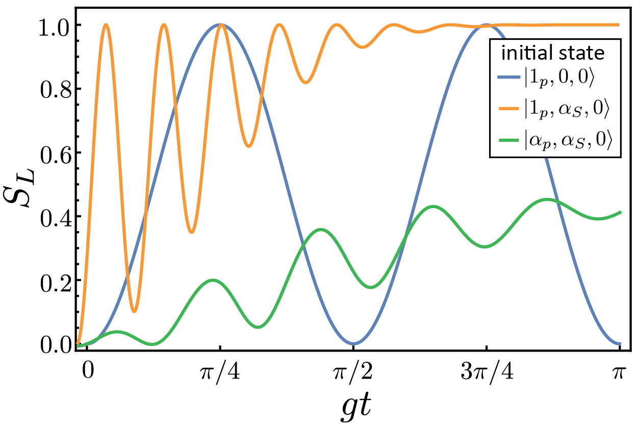
Figure 1: Phonon linear entropy for experimentally accessible initial states. Coherent state amplitudes $\alpha_{p}=1.0$ and $\alpha_{S}=4.6$. For the single pump photon initial states, the linear entropy is scaled by a factor $2$ so that $S_{L}$ varies between 0 and 1. $S_{L}=1$ indicates maximal phonon-photon entanglement.

Preparing and measuring quantum states of a mechanical mode: Leveraging phonon-photon entanglement shown by Eq. (7) and Fig. 1, the phonon mode can be projected into a large variety of highly nonclassical states through conditional measurements of the optical fields. By applying the projective operator $\hat{P}=|\varphi_{p},\varphi_{S}\rangle\langle\varphi_{p},\varphi_{S}|$ to $|\psi(t)\rangle$, we obtain the phonon wavefunction $|\psi_{ph}[\varphi_{p},\varphi_{S},t)\rangle\equiv\langle\varphi_{p},\varphi_{S}|\psi(t)\rangle$ resulting from the conditional measurement of the optical fields with measurement outcomes given by $\varphi_{p}$ and $\varphi_{S}$ for the pump and Stokes modes respectively. For example, for homodyne detection $\varphi_{p}$ represents the measured complex coherent state amplitude of the pump mode, or a photon number resolving measurement $\varphi_{p}$ indicates the measured number of pump photons.

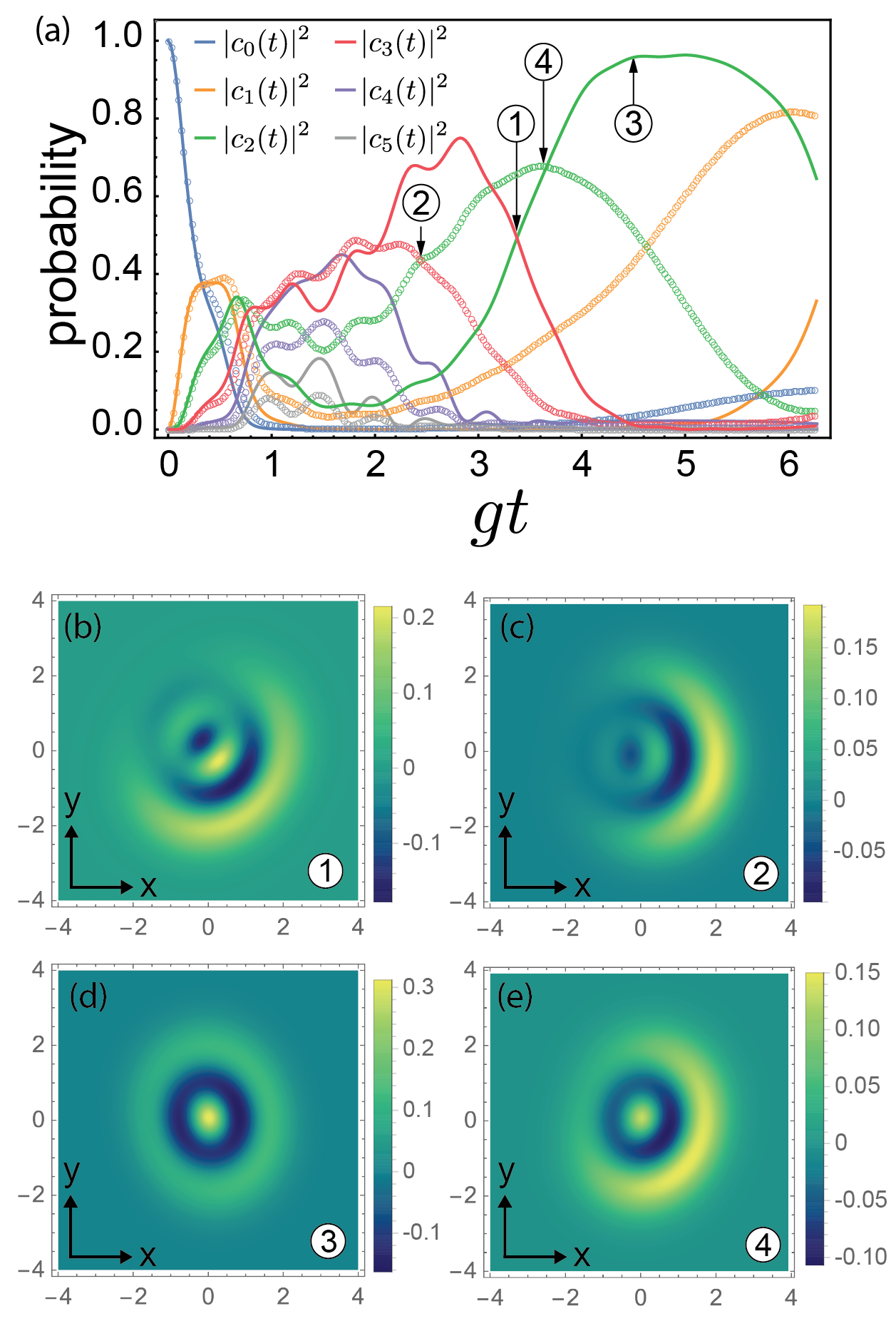
Figure 2: Conditional quantum state preparation through homodyne measurements of the optical field. The initial state is $|\alpha_{p},\alpha_{S},0\rangle$ and the optical fields are measured in state $|\bar{\alpha}_{p},\bar{\alpha}_{S}\rangle$ at a later time. For $\alpha_{p}=0.74,\ \alpha_{S}=5.6,\ \bar{\alpha}_{p}=0.01,\ \bar{\alpha}_{S}=5.65\exp\{i0.3\pi\}$. (a) Phonon Fock state probabilities calculated from Eq. (11) (solid lines) and using a numerical master equation solver with damping for both pump and Stokes modes of $\gamma=0.25g$ (open circles). (b)-(e) Wigner functions for targeted phonon states with and without optical losses. States approximating $|\psi_{ph}\rangle\approx(|2\rangle+|3\rangle\exp\{i\phi\})/\sqrt{2})$ shown in (b) $gt=3.37$, denoted by $①$ (lossless) and (c) $gt=2.63$, denoted by $②$ (optical losses). States approximating $|\psi_{ph}\rangle\approx|2\rangle$ shown in (d) $gt=4.5$, denoted by $③$ (lossless), and (e) $gt=3.63$, denoted by $④$ (optical losses). Fidelities for state preparation with losses are 72% for (c) and 67% for (e).

Using homodyne detection, a projective measurement of the amplitude and phase of the optical modes in the interaction picture collapses the phonon wavefunction into the superposition of Fock states given by $|\psi_{ph}[\bar{\alpha}_{p},\bar{\alpha}_{S},t)\rangle=\sum_{k=0}^{\infty}c_{k}(t)|k\rangle.$ Here, the unnormalized probability amplitudes $c_{k}(t)$ are given by

$$c_{k}(t)=\sum_{n=k}^{\infty} \sum_{m=0}^{\infty}\frac{\alpha_{p}^{n}(\bar{\alpha}_{p}^{*})^{n-k}\alpha_{S}^{m}(\bar{\alpha}_{S}^{*})^{m+k}}{\sqrt{n!}\sqrt{(n-k)!}\sqrt{m!}\sqrt{(m+k)!}}$$ (11)

$$\times e^{-\frac{1}{2}(|\alpha_{p}|^{2}+|\bar{\alpha}_{p}|^{2}+|\alpha_{S}|^{2}+|\bar{\alpha}_{S}|^{2})}A_{n,m,k}(t),$$

and $\bar{\alpha}_{p}$ and $\bar{\alpha}_{S}$ are the measured complex amplitudes for the pump and Stokes modes. For a given experimental configuration (i.e., input laser amplitudes and measured final states), examination of the phonon Fock state probabilities as a function of time identify how certain states can be prepared (e.g., see Fig. 2(a)). Such conditional measurements can collapse the phonon into a highly nonclassical state as shown in Fig. 2(b)-(e). For example, in Fig. 2(b) the system occupies a nearly perfect superposition $|\psi_{ph}\rangle\approx(|2\rangle+|3\rangle\exp\{i\phi\})/\sqrt{2}$. Accounting for decoherence caused by optical losses, a master equation simulation Johansson et al. (2012) shows that this state can be achieved with 72% fidelity when the optical decay rates $\gamma=0.25g$ (see Supplementary Information E). With the large optomechanical coupling rates achievable in optomechanical crystals Chan et al. (2009) ($\sim$ 9 MHz), it is conceivable that future devices reach regimes where $\gamma\ll g$. However, even with larger optical losses, interesting states can still be accessed. By adjusting the initial optical state, entanglement generation can be accelerated so that targeted quantum states can be prepared at times $t<1/\gamma$ (example below). Beyond this example, a tremendous range of nonclassical states become accessible by varying the amplitude and phases of initial and final photonic states as well as the measurement time.

We can also use Eq. (7) to identify opportunities for quantum state synthesis using conditional photon number resolving measurements. For example, when $|\psi(0)\rangle=|\alpha_{p},\alpha_{S},0\rangle$ and when a single photon is measured in the pump and Stokes modes at time $t$, the phonon wavefunction collapses into the superposition of ground and excited states, expressed in unnormalized form as

$$|\psi_{ph}[1_{p},1_{s},t)\rangle\!=\!\mathcal{N}\big{[}\alpha_{S}\cos(\sqrt{2}gt)|0\rangle\!-\!\frac{i\alpha_{p}}{\sqrt{6}}\sin(\sqrt{6}gt)|1\rangle\big{]}$$ (12)

where $\mathcal{N}=\alpha_{p}\mathcal{P}_{0}\mathcal{S}_{0}$. Although nondeterministic, manipulation of the initial state affords some control over the phonon wavefunction, e.g., by setting the amplitude $\alpha_{S}$ to zero the mechanical mode is guaranteed to be in a single phonon state.

Using single photon detection, we can illustrate how quantum state synthesis can be achieved with optical losses. Figure 3 shows the phonon Fock state probabilities, computed using Eq. (7) (solid lines) and a master equation solver (open circles), along with the phonon Wigner functions for the simulation with optical losses at selected times when a single Stokes photon is measured and the pump is measured using homodyne detection. This figure shows that even with optical decay rates of $50g$, a coherent superposition between ground and excited states and a single phonon state can be prepared with respective fidelities of 97% and 92%.

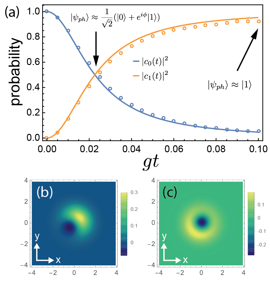
Figure 3: Phonon Fock state probabilities (a) and Wigner functions (b)-(c) after single photon measurement in the Stokes mode and homodyne measurement in the pump mode. Fock state probabilities computed using Eq. (7) (lines) and a master equation solver including optical losses of decay rate $\gamma=50g$ (open circles). Plotted Wigner functions include the effects of optical losses. The inital state is $|\alpha_{p},\alpha_{S},0\rangle$ with $\alpha_{p}=4.41$ and $\alpha_{S}=0.1$, and the measured complex amplitude of the pump is $\bar{\alpha}_{p}=3.7$.

Even in the absence of conditional measurements, the mechanical oscillator can evolve into nonclassical states, leading to a form of deterministic state synthesis. In this case, the phonon mode is described by a reduced density matrix $\hat{\rho}_{red}(t)=\sum_{k,k^{\prime}=0}^{\infty}\rho_{kk^{\prime}}(t)|k\rangle\langle k^{\prime}|$ with matrix element given by

$$\rho_{kk^{\prime}}(t)=\sum_{n=0}^{\infty}\sum_{m=\kappa}^{\infty} \mathcal{P}_{n+k}\mathcal{P}^{*}_{n+k^{\prime}}\mathcal{S}_{m-k}\mathcal{S}^{*}_{m-k^{\prime}}$$ (13)

$$\times A_{n+k,m-k,k}(t)A^{*}_{n+k^{\prime},m-k^{\prime},k^{\prime}}(t)$$

where $\kappa={\rm max}(k,k^{\prime})$. For a specific initial state, Fig. 4 (a) illustrates how the Fock state probabilities for the phonon evolve in time, showing how a variety of macroscopic superposition states can be prepared Fig. 4. We emphasize that this behavior is a consequence of the quantum nonlinearity. Importantly, without the effects backreaction on the pump and the Stokes modes (e.g., pump depletion) provided by the nonlinear dynamics produced by Eq. (1), the phonon would evolve into a thermal or coherent state Gerry et al. (2005), and negativity of the Wigner function would not be possible.

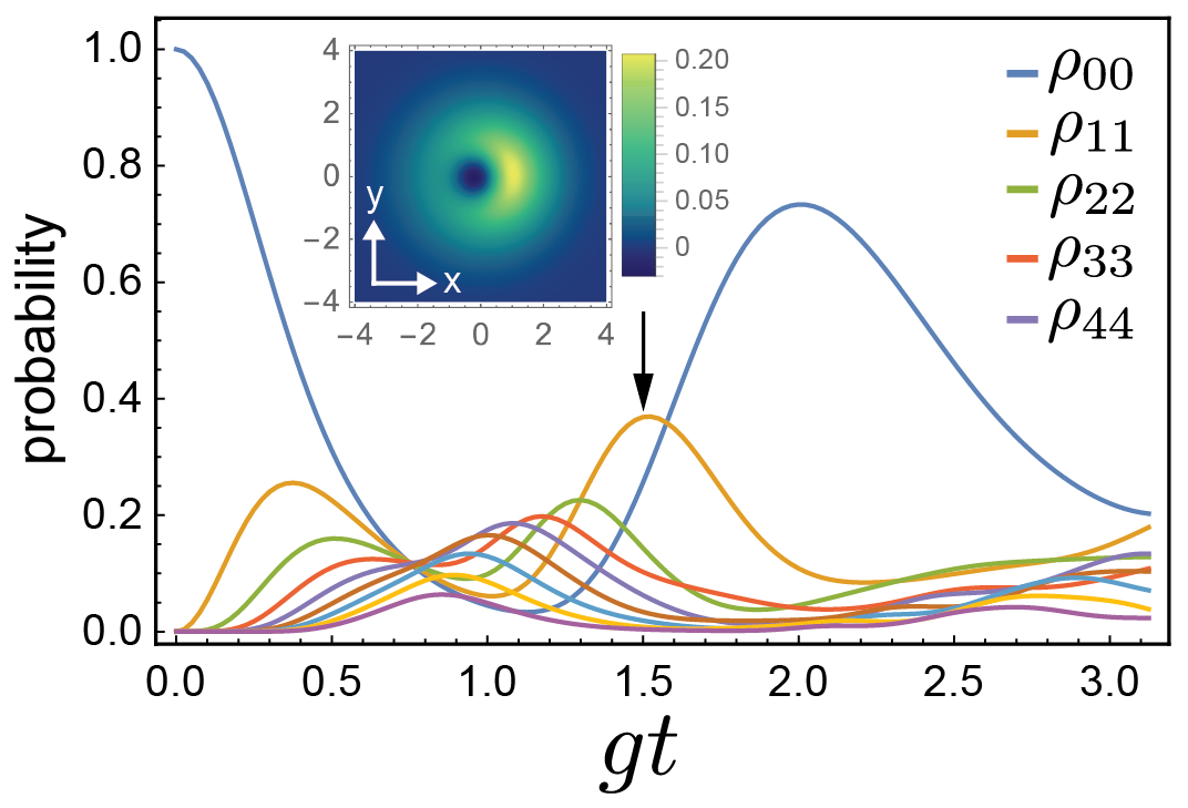
Figure 4: Phonon occupation number probabilities when optical fields are traced out (i.e., not measured). The initial state is $|\alpha_{p},\alpha_{S},0\rangle$ with $\alpha_{p}=2.4$ and $\alpha_{S}=0.25$. Inset: phonon Wigner function at $gt=1.5$.

Quantum state readout: In addition to providing a means to prepare quantum states of mechanical motion, $H_{int}$ also enables state manipulation, transfer and readout. When the Stokes mode is a large amplitude coherent state (i.e., $|\alpha_{S}|\gg 1$), the $\exp\{-iH_{int}t/\hbar\}$ is well-approximated by the beam splitter transformation, transferring and entangling quantum states between the phononic and photonic domains Aspelmeyer et al. (2014). Consider a phonon wavefunction given by a superposition of ground and excited states $|\psi_{ph}\rangle=c_{0}|0\rangle+c_{1}|1\rangle$. Equation (12) shows how this state can be prepared by conditional photon number resolving measurements. For the pump mode in the vacuum state and Stokes mode in a coherent state, the system wavefunction at time $t$ is

$$|\psi(t)\rangle=\sum_{m=0}^{\infty}\mathcal{S}_{m}\bigg{[} c_{0}|0,m,0\rangle+c_{1}\cos(\sqrt{m}gt)|0,m,1\rangle$$

$$-ic_{1}\sin(\sqrt{m}gt)|1,m-1,0\rangle\bigg{]}.$$ (14)

Under these assumptions, $\mathcal{S}_{m}$ is peaked at $m\sim|\alpha_{S}|^{2}$ with a standard deviation $\Delta m=|\alpha_{S}|$, allowing the arguments of the cosine and sine terms to be approximated by $\sqrt{m}gt\approx|\alpha_{S}|gt$ when $gt\ll 1$. Assuming the phase of $\alpha_{S}$ is $\pi/2$, these approximations give

$$|\psi(t)\rangle\approx c_{0}|0,\alpha_{S},0\rangle+c_{1} \big{[}\cos(|\alpha_{S}|gt)|0,\alpha_{S},1\rangle$$

$$+\sin(|\alpha_{S}|gt)|1,\alpha_{S},0\rangle\big{]},$$ (15)

providing a “state-swap” when $t=t_{\pi}\equiv\pi/(2|\alpha_{S}|g)$. For this generalized tripartite optomechanical “$\pi$-pulse”, $|\psi(t_{\pi})\rangle\approx(c_{0}|0\rangle+c_{1}|1\rangle)\otimes|\alpha_{S},0\rangle$ showing how a quantum state in the mechanical domain can be transferred to the optical domain where quantum state tomography can be performed. This result also shows how an optomechanical $\pi/2$-pulse ($|\alpha|gt_{\pi/2}=\pi/4$) can be used to prepare an entangled superposition of the pump and phonon. For $c_{0}=0$ and $c_{1}=1$, a phonon-photon Bell state is produced

$$|\psi(t_{\pi/2})\rangle\!\approx\!\frac{1}{\sqrt{2}} \big{[}|0,\alpha_{S},1\rangle\!-\!ie^{i\varphi}|1,\alpha_{S},0\rangle\big{]}$$ (16)

where $\varphi$ is the phase of the Stokes mode. By sequencing these pulses, multimode optomechanical analogs of Ramsey interference and spin echo can be performed. While these results, focus on the $|\alpha_{S}|\gg 1$ limit, Eq. (16) can be used to describe general “state-swap” dynamics.

Conclusion: In this letter we have shown how three-mode optomechanical coupling can be used to prepare and measure quantum states of a mechanical oscillator. A formal solution to the Schrodinger equation for this system yields highly entangled photon-phonon states, even with classically prepared initial states. Levering this entanglement, conditional measurements on the optical fields can generate a wide variety of quantum states of the mechanical oscillator. For quantum state tomography, this tripartite coupling permits the optomechanical equivalent of $\pi/2$- and $\pi$-pulses that can be used to entangle optical and mechanical states as well as transfer quantum information between the electromagnetic and mechanical domains. With the long lifetimes at cryogenic temperatures, natural interface with telecommunications and radio frequency wavelengths, and large effective masses of phonon modes, our results may enable new ways to manipulate quantum information stored in mechanical oscillators as well as tests of the foundations of quantum physics.

This work was supported by NSF Award 2145724 and ¡MIRA! ER Funds. The authors thank In$\rm{\grave{e}}$s Monta$\rm{\tilde{n}}$o, Daniel Reiche, and Shruti Puri for stimulating discussions.

Appendix A Formal equivalence between the multimode optomechanical Hamiltonian and the Jaynes-Cummings model

Leveraging the conservation of the number of pump photons and phonons and the Schwinger oscillator model of angular momentum Schwinger1952 , a formal analogy between the multimode optomechanical Hamiltonian and the Jaynes-Cummings model Jaynes and Cummings (1963) can be derived. To reveal this relationship, we define the following pseudospin operators

$$\hat{N}=(\hat{n}_{p}+\hat{n}_{b})/2$$ (17)

$$S_{z}=(\hat{n}_{p}-\hat{n}_{b})/2$$ (18)

$$S_{-}=a_{p}b^{\dagger}$$ (19)

$$S_{+}=a_{p}^{\dagger}b$$ (20)

where $\hat{n}_{p}$ and $\hat{n}_{b}$ are the number operators for the pump and phonon modes respectively. The commutation relations of $a_{p}$ and $b$ show that the pseudospin operators obey the relations

$$[\hat{N},S_{z}]=0$$ (21)

$$[S_{z},S_{\pm}]=\pm S_{\pm}$$ (22)

$$[S_{+},S_{-}]=2S_{z}.$$ (23)

Furthermore, one can show that $N$, the eigenvalue for $\hat{N}$, plays the role for the total spin, that these operators have all of the expected effects on Fock states $|n_{p},n_{b}\rangle$ where the eigenvalues of $S_{z}$, $m\equiv(n_{p}-n_{b})/2$, correspond with azimuthal component of the pseudospin along the “z-axis”. For example, using $N$ and $m$, a generic Fock state $|n_{p},n_{b}\rangle$ can be formally expressed as $|N,m\rangle$ ($n_{p}=N+m$ and $n_{b}=N-m$) where the operators above have act in a manner analogous to a spin system:

$$S_{z}|N,m\rangle =m|N,m\rangle$$ (24)

$$S_{\pm}|N,m\rangle =\sqrt{N\pm m+1}\sqrt{N\mp m}|N,m\pm 1\rangle$$ (25)

$${\bf S}^{2}|N,m\rangle =(S_{z}^{2}-S_{z}+S_{+}S_{-})|N,m\rangle$$ (26)

$$=N\left(N+1\right)|N,m,j\rangle.$$ (27)

Using these operators and the phase matching conditions one can show that

$$H \to\hbar(\omega_{p}+\Omega)N+\hbar\omega_{S}S_{z}+\hbar\omega_{S}a^{\dagger}_{S}a_{S}+\hbar g(S_{-}a^{\dagger}_{S}+S_{+}a_{S})$$ (28)

demonstrating the equivalence between the multimode Hamiltonian and the JC model when $N$ is fixed. In general, initial states that can be prepared in the lab will contain a superposition of different $N$-states, such as coherent states. Therefore, the multimode optomechanical dynamics of realistic systems is complex, involving several pseudospins, with distinct spin $N$, interacting with a bosonic mode.

Appendix B Diagonalization of ${\bf M}_{nm}$

The formal solution to Eq. (3) can be obtained by diagonalizing ${\bf M}_{nm}$. By solving the eigenvalue equation ${\bf M}_{nm}\cdot\vec{E}_{nm,k}={\Omega}_{nm,k}\vec{E}_{nm,k}$, where $\vec{E}^{*}_{nm,k}\cdot\vec{E}_{nm,k^{\prime}}=\delta_{k,k^{\prime}}$, the eigenvalues can be obtained as well as the unitary matrix ${\bf V}_{nm}$. Comprising a matrix of the normalized eigenvectors of ${\bf M}_{nm}$, the definition of ${\bf V}_{nm}$

$${\bf V}_{nm}=\begin{pmatrix}\vec{E}_{nm,n},&\vec{E}_{nm,n-1},&\ldots&\vec{E}_{nm,0}\end{pmatrix}.$$ (29)

For example, for $n_{p}+n_{b}=1$, the normalized eigenvectors are

$$\vec{E}_{1m,1}=\frac{1}{\sqrt{2}}\begin{pmatrix}1\\ 1\end{pmatrix},\quad\vec{E}_{1m,0}=\frac{1}{\sqrt{2}}\begin{pmatrix}-1\\ 1\end{pmatrix}$$ (30)

giving ${\bf V}_{1m}$

$${\bf V}_{1m}=\frac{1}{\sqrt{2}}\begin{pmatrix}1&-1\\ 1&1\end{pmatrix}.$$ (31)

Using ${\bf V}_{1m}$ to diagonalize ${\bf M}_{1m}$ we obtain the diagonal matrix of eigenvalues ${\bf\Omega}_{1m}$

$${\bf V}_{1m}^{\dagger}\cdot{\bf M}_{1m}\cdot{\bf V}_{1m}\equiv{\bf\Omega}_{1m}=g\sqrt{m+1}\begin{pmatrix}1&0\\ 0&-1\end{pmatrix}.$$ (32)

Appendix C Probability amplitude time-dynamics

Here we list the first few terms $A_{n,m,k}(t)$. By solving Eq. (3), assuming the phonon is initially in the ground state, we find

$$A_{0,m,0}(t)=1$$ (33)

$$A_{1,m,0}(t)=\cos(\sqrt{m+1}gt)$$ (34)

$$A_{1,m,1}(t)=-i\sin(\sqrt{m+1}gt)1$$ (35)

$$A_{2,m,0}(t)=\frac{2+m+(1+m)\cos(\sqrt{4m+6}gt)}{3+2m}$$ (36)

$$A_{2,m,1}(t)=-i\sqrt{\frac{1+m}{3+2m}}\sin(\sqrt{4m+6}gt)$$ (37)

$$A_{2,m,2}(t)=-2\frac{\sqrt{(1+m)(2+m)}}{3+2m}\sin^{2}(\sqrt{m+3/2}gt)$$ (38)

Appendix D General Expression for the Wigner function

The phonon Wigner function is given by

$$W(\alpha)=\frac{1}{2\pi^{2}}\int d^{2}\xi\ e^{\alpha\xi^{*}-\alpha^{*}\xi}{\rm Tr}[\hat{\rho}D(\xi)]$$ (39)

where $\alpha\equiv(x+iy)/\sqrt{2}$, $x$ and $y$ are dimensionless position and momentum quadratures, and $D(\xi)$ is the phonon displacement operator Gerry et al. (2005). Here, $\hat{\rho}$ is either reduced phonon density matrix, or the density matrix obtained after conditional measurement of the optical fields.

For a general state expressed in the Fock basis (i.e., $\rho_{kk^{\prime}}$), the Wigner function is given by

$$W(\alpha)=\frac{1}{\pi}\sum_{k,k^{\prime}=0}^{\infty}\frac{(-1)^{k}2^{k^{\prime}-k}}{\sqrt{k!}\sqrt{k^{\prime}!}}(\partial_{\alpha}\!-\!2\alpha^{*})^{k}\alpha^{k^{\prime}}e^{-2\alpha\alpha^{*}}\rho_{kk^{\prime}}$$ (40)

where $\rho_{kk^{\prime}}=c_{k}c_{k^{\prime}}^{*}$ for a pure state and $c_{k}$ is the phonon probability amplitude for the $k$th Fock state.

For the case where the optical fields are conditionally measured, the general expression for the phonon Wigner function can be computed by making the following replacement in Eq. (39) is given by

$${\rm Tr}[\hat{\rho}D(\xi)]\to\langle\psi_{ph}[\varphi_{p},\varphi_{S},t)|D(\xi)|\psi_{ph}[\varphi_{p},\varphi_{S},t)\rangle.$$ (41)

Appendix E Effects of optical losses from master equation simulations

For the assessment of decoherence caused by optical losses, we simulate the quantum dynamics of this tripartite optomechanical system Johansson et al. (2012). We solve the Linblad form of the the master equation, capturing the decay of both optical modes at a rate $\gamma$ given by

$$\dot{\rho}=-\frac{i}{\hbar}[H,\rho]+\frac{\gamma}{2}\sum_{j=p,S}[2a_{j}\rho a^{\dagger}_{j}-a^{\dagger}_{j}a_{j}\rho-\rho a^{\dagger}_{j}a_{j}].$$ (42)

Given the high frequency of the photon modes, Eq. (42) assumes a bath temperature of zero.

References

- Marshall et al. (2003) W. Marshall, C. Simon, R. Penrose, and D. Bouwmeester, Physical Review Letters 91, 130401 (2003).
- Goryachev et al. (2012) M. Goryachev, D. L. Creedon, E. N. Ivanov, S. Galliou, R. Bourquin, and M. E. Tobar, Applied Physics Letters 100, 243504 (2012).
- Goryachev et al. (2013) M. Goryachev, D. L. Creedon, S. Galliou, and M. E. Tobar, Physical Review Letters 111, 085502 (2013).
- Galliou et al. (2013) S. Galliou, M. Goryachev, R. Bourquin, P. Abbé, J. P. Aubry, and M. E. Tobar, Scientific reports 3, 2132 (2013).
- Lo et al. (2016) A. Lo, P. Haslinger, E. Mizrachi, L. Anderegg, H. Müller, M. Hohensee, M. Goryachev, and M. E. Tobar, Physical Review X 6, 011018 (2016).
- Tobar (2017) M. E. Tobar, New Journal of Physics 19, 091001 (2017).
- Renninger et al. (2018) W. Renninger, P. Kharel, R. Behunin, and P. Rakich, Nature Physics (2018), 10.1038/s41567-018-0090-3.
- Kharel et al. (2018) P. Kharel, Y. Chu, M. Power, W. H. Renninger, R. J. Schoelkopf, and P. T. Rakich, APL Photonics 3, 066101 (2018).
- Eichenfield et al. (2009a) M. Eichenfield, R. Camacho, J. Chan, K. J. Vahala, and O. Painter, Nature 459, 550 (2009a).
- Eichenfield et al. (2009b) M. Eichenfield, J. Chan, R. M. Camacho, K. J. Vahala, and O. Painter, Nature 462, 78 (2009b).
- Weaver et al. (2017) M. J. Weaver, F. Buters, F. Luna, H. Eerkens, K. Heeck, S. de Man, and D. Bouwmeester, Nature communications 8, 1 (2017).
- Campbell et al. (2021) W. M. Campbell, B. T. McAllister, M. Goryachev, E. N. Ivanov, and M. E. Tobar, Physical Review Letters 126, 071301 (2021).
- MacCabe et al. (2020) G. S. MacCabe, H. Ren, J. Luo, J. D. Cohen, H. Zhou, A. Sipahigil, M. Mirhosseini, and O. Painter, Science 370, 840 (2020).
- Pechal et al. (2018) M. Pechal, P. Arrangoiz-Arriola, and A. H. Safavi-Naeini, Quantum Science and Technology 4, 015006 (2018).
- Chu et al. (2017) Y. Chu, P. Kharel, W. H. Renninger, L. D. Burkhart, L. Frunzio, P. T. Rakich, and R. J. Schoelkopf, Science 358, 199 (2017).
- Chu et al. (2018) Y. Chu, P. Kharel, T. Yoon, L. Frunzio, P. T. Rakich, and R. J. Schoelkopf, Nature 563, 666 (2018).
- Wollack et al. (2022) E. A. Wollack, A. Y. Cleland, R. G. Gruenke, Z. Wang, P. Arrangoiz-Arriola, and A. H. Safavi-Naeini, Nature 604, 463 (2022).
- Manenti et al. (2017) R. Manenti, A. F. Kockum, A. Patterson, T. Behrle, J. Rahamim, G. Tancredi, F. Nori, and P. J. Leek, Nature communications 8, 1 (2017).
- Reed et al. (2017) A. Reed, K. Mayer, J. Teufel, L. Burkhart, W. Pfaff, M. Reagor, L. Sletten, X. Ma, R. Schoelkopf, E. Knill, et al., Nature Physics 13, 1163 (2017).
- Ghirardi et al. (1990) G. C. Ghirardi, P. Pearle, and A. Rimini, Physical Review A 42, 78 (1990).
- Percival (1994) I. C. Percival, Proceedings of the Royal Society of London. Series A: Mathematical and Physical Sciences 447, 189 (1994).
- Manley et al. (2020) J. Manley, D. J. Wilson, R. Stump, D. Grin, and S. Singh, Physical review letters 124, 151301 (2020).
- Diósi (1989) L. Diósi, Physical Review A 40, 1165 (1989).
- Penrose (2014) R. Penrose, Foundations of Physics 44, 557 (2014).
- O’Connell et al. (2010) A. D. O’Connell, M. Hofheinz, M. Ansmann, R. C. Bialczak, M. Lenander, E. Lucero, M. Neeley, D. Sank, H. Wang, M. Weides, et al., Nature 464, 697 (2010).
- Palomaki et al. (2013) T. Palomaki, J. Teufel, R. Simmonds, and K. W. Lehnert, Science 342, 710 (2013).
- Aref et al. (2016) T. Aref, P. Delsing, M. K. Ekström, A. F. Kockum, M. V. Gustafsson, G. Johansson, P. J. Leek, E. Magnusson, and R. Manenti, in Superconducting devices in quantum optics (Springer, 2016) pp. 217–244.
- Nielsen et al. (2017) W. H. P. Nielsen, Y. Tsaturyan, C. B. Møller, E. S. Polzik, and A. Schliesser, Proceedings of the National Academy of Sciences 114, 62 (2017).
- Hong et al. (2017) S. Hong, R. Riedinger, I. Marinković, A. Wallucks, S. G. Hofer, R. A. Norte, M. Aspelmeyer, and S. Gröblacher, Science 358, 203 (2017).
- Sletten et al. (2019) L. R. Sletten, B. A. Moores, J. J. Viennot, and K. W. Lehnert, Physical Review X 9, 021056 (2019).
- Satzinger et al. (2018) K. J. Satzinger, Y. Zhong, H.-S. Chang, G. A. Peairs, A. Bienfait, M.-H. Chou, A. Cleland, C. R. Conner, É. Dumur, J. Grebel, et al., Nature 563, 661 (2018).
- Aspelmeyer et al. (2014) M. Aspelmeyer, T. J. Kippenberg, and F. Marquardt, Reviews of Modern Physics 86, 1391 (2014).
- Mancini et al. (1997) S. Mancini, V. Man’ko, and P. Tombesi, Physical Review A 55, 3042 (1997).
- Bose et al. (1997) S. Bose, K. Jacobs, and P. Knight, Physical Review A 56, 4175 (1997).
- Kharel et al. (2019) P. Kharel, G. I. Harris, E. A. Kittlaus, W. H. Renninger, N. T. Otterstrom, J. G. Harris, and P. T. Rakich, Science advances 5, eaav0582 (2019).
- Rakich et al. (2012) P. T. Rakich, C. Reinke, R. Camacho, P. Davids, and Z. Wang, Physical Review X 2, 11008 (2012).
- Kharel et al. (2016) P. Kharel, R. O. Behunin, W. H. Renninger, and P. T. Rakich, Physical Review A 93, 063806 (2016).
- Jaynes and Cummings (1963) E. T. Jaynes and F. W. Cummings, Proceedings of the IEEE 51, 89 (1963).
- Arfken and Weber (2005) G. B. Arfken and H. J. Weber, Mathematical methods for physicists (Elsevier Academic Press; 6th edition, 2005).
- Shore and Knight (1993) B. W. Shore and P. L. Knight, Journal of Modern Optics 40, 1195 (1993).
- Johansson et al. (2012) J. R. Johansson, P. D. Nation, and F. Nori, Computer Physics Communications 183, 1760 (2012).
- Chan et al. (2009) J. Chan, M. Eichenfield, R. Camacho, and O. Painter, Optics Express 17, 3802 (2009).
- Gerry et al. (2005) C. Gerry, P. Knight, and P. L. Knight, Introductory quantum optics (Cambridge university press, 2005).
- (44) J. Schwinger, Unpublished report, NYO-3071 (1952).