Multi-element metamaterial’s design through the relaxed micromorphic model

Exploring the dynamical response of mechanical metamaterials has gathered increasing attention in the last decades, enabling the design of microstructures exotically interacting with elastic waves (focusing, channeling, band-gaps, negative refraction, cloaking, and many more). Yet, the application and use of such metamaterials in engineering practice is still deficient due to the lack of effective models unveiling metamaterials’ interactions with more classical materials at finite scales. In this paper, we show that the relaxed micromorphic model can bring an answer to this open problem and can be effectively used to explore and optimize metamaterials’ structures consisting of metamaterials’ and classical materials’ bricks of finite size. We investigate two examples, namely a double-shield structure that can be used to widen the frequency range for which the internal region can be protected and a multiple-shield structure that optimizes both the screening of the regions internal to the single shields and of the zones exterior to the shields themselves. The exploration of these complex meta-structures has been enabled by the finite element implementation of the relaxed micromorphic model that predicts their response at a fraction of the computational cost when compared to classical simulations.

1 Introduction

Metamaterials are architectured materials whose mechanical properties go beyond those of classical materials thanks to local resonance or Bragg scattering phenomena occurring in their heterogeneous microstructure. This micro-heterogeneity allows them to show exceptional mechanical features such as negative Poisson’s ratio [33], twist and bend in response to being pushed or pulled [26, 50, 51], band-gaps [34, 58, 6, 10, 19, 31, 28, 64], cloaking [9, 42, 48, 41], focusing [29, 14], channeling [30, 56, 7, 59, 38], negative refraction [62, 7, 64, 55, 35, 43], and many others.

In the last two centuries, the advancement of knowledge on finite-size classical materials modeling has enabled the design of engineering structures (buildings, bridges, airplanes, cars, etc.) resisting to static and dynamic loads.

Today, while the modeling of infinite-size metamaterials is achievable via reliable homogenization techniques, we must acknowledge that such methods are not optimized to deal with finite-size metamaterials’ modeling, mainly due to the lack of well-posed homogenized boundary conditions [11, 61, 13, 60, 63, 8, 54]. This conceptual gap has prevented us to explore structures made up of both metamaterials and classical materials, and optimize them towards efficient wave control and energy recovery.

Other enriched models, such as strain-gradient, micropolar, Cosserat or classical micromorphic [17, 12, 16, 4, 22, 44, 23, 24, 3, 21, 37, 25] can be used to describe dispersive behaviours or even higher-frequency modes. However, their use has not been widespread for modeling metamaterials due to limited additional degrees of freedom or to an excessive number of elastic parameters.

In this paper, we show that the mechanical response of finite-size metamaterials can be explored using an elastic- and inertia-augmented micromorphic model (relaxed micromorphic) which is able to describe the main metamaterials’ fingerprint characteristics (anisotropy, dispersion, band-gaps, size-effects, etc.), while keeping a reduced structure (free of unnecessary parameters). This model can be linked a posteriori to real metamaterials’ microstructures via a fitting approach. The reduced model’s structure, coupled with the introduction of well-posed boundary conditions, allows us to unveil the dynamic response of metamaterials’ bricks of finite size and complex shapes. Playing LEGO with such bricks can enable the design of surprising structures, combining metamaterials and classical materials, actively controlling noise, vibrations, seismic waves, and many others, while being able to recover energy.

At present, the response of finite-size metamaterials’ structures is mostly explored via direct Finite Element (FEM) simulations implementing all microstructures’ details (e.g., [32, 40, 5, 20]). Despite the accurate static and dynamic response that these simulations can provide, they suffer from unsustainable computational costs, already for rather simple structure topoligies. Therefore, the exploration of large-scale structures combining metamaterials’ and classical materials’ bricks of different type, size and shape, has been until today out of reach.

In this paper, we lay the basis to overcome this stagnation point and we show how the thorough application of the relaxed micromorphic model can open the way to the design of multi-metamaterial’s structures that can control elastic wave propagation. We will focus here on protection devices (shielding), but similar approach could be adopted for many other applications.

2 The relaxed micromorphic model: constitutive laws,
equilibrium equations, and boundary conditions

In this section, we present the constitutive relations, the equilibrium equations, and the associated boundary conditions for the relaxed micromorphic model [47, 57, 2, 27, 36, 46, 45]. The equilibrium equations and the boundary conditions can be derived by means of a variational approach through the associated Lagrangian

$$\mathcal{L}\left(\dot{u},\nabla\dot{u},\dot{P},\text{Curl}\dot{P},\nabla u,P,\text{Curl}P\right)\coloneqq K\left(\dot{u},\nabla\dot{u},\dot{P}\right)-W\left(\nabla u,P,\text{Curl}P\right)\ ,$$ (1)

where $K$ and $W$ are the kinetic and strain energy, respectively [57], defined as:

$$K\left(\dot{u},\nabla\dot{u},\dot{P}\right)= \dfrac{1}{2}\rho\,\langle\dot{u},\dot{u}\rangle+\dfrac{1}{2}\langle\mathbb{J}_{\rm m}\,\text{sym}\,\dot{P},\text{sym}\,\dot{P}\rangle+\dfrac{1}{2}\langle\mathbb{J}_{\rm c}\,\text{skew}\,\dot{P},\text{skew}\,\dot{P}\rangle$$

$$+\dfrac{1}{2}\langle\mathbb{T}_{\rm e}\,\text{sym}\nabla\dot{u},\text{sym}\nabla\dot{u}\rangle+\dfrac{1}{2}\langle\mathbb{T}_{\rm c}\,\text{skew}\nabla\dot{u},\text{skew}\nabla\dot{u}\rangle$$ (2)

$$+\dfrac{1}{2}\langle\mathbb{M}_{\rm s}\,\text{sym}\,\text{Curl}\,\dot{P},\text{sym}\,\text{Curl}\,\dot{P}\rangle+\dfrac{1}{2}\langle\mathbb{M}_{\rm a}\,\text{skew}\,\text{Curl}\,\dot{P},\text{skew}\,\text{Curl}\,\dot{P}\rangle\,,$$

$$W\left(\nabla u,P,\text{Curl}P\right)= \dfrac{1}{2}\langle\mathbb{C}_{\rm e}\,\text{sym}\left(\nabla u-\,P\right),\text{sym}\left(\nabla u-\,P\right)\rangle$$

$$+\dfrac{1}{2}\langle\mathbb{C}_{\rm c}\,\text{skew}\left(\nabla u-\,P\right),\text{skew}\left(\nabla u-\,P\right)\rangle$$

$$+\dfrac{1}{2}\langle\mathbb{C}_{\rm micro}\,\text{sym}\,P,\text{sym}\,P\rangle$$

$$+\dfrac{1}{2}\langle\mathbb{L}_{\rm s}\,\text{sym}\,\text{Curl}P,\text{sym}\,\text{Curl}\,P\rangle+\dfrac{1}{2}\langle\mathbb{L}_{\rm a}\,\text{skew}\,\text{Curl}P,\text{skew}\,\text{Curl}\,P\rangle\,,$$

where $u\in\mathbb{R}^{3}$ is the macroscopic displacement field, $P\in\mathbb{R}^{3\times 3}$ is the non-symmetric micro-distortion tensor, $\rho$ is the macroscopic apparent density, $\mathbb{J}_{\rm m}$, $\mathbb{J}_{\rm c}$, $\mathbb{T}_{\rm e}$, $\mathbb{T}_{\rm c}$, $\mathbb{M}_{\rm s}$, $\mathbb{M}_{\rm a}$, are 4th order micro-inertia tensors, and $\mathbb{C}_{\rm e}$, $\mathbb{C}_{\rm m}$, $\mathbb{C}_{\rm c}$, $\mathbb{L}_{\rm s}$, $\mathbb{L}_{\rm a}$ are 4th order elasticity tensors. Further details on the definition of these tensors can be found in [52, 57]. In the tetragonal symmetry case, these tensors in Voigt notation can be expressed as follows

$$\mathbb{C}_{\rm e} =\begin{pmatrix}\lambda_{\rm e}+2\mu_{\rm e}&\lambda_{\rm e}&\star&\dots&0\\ \lambda_{\rm e}&\lambda_{\rm e}+2\mu_{\rm e}&\star&\dots&0\\ \star&\star&\star&\dots&0\\ \vdots&\vdots&\vdots&\ddots&\\ 0&0&0&&\mu_{\rm e}^{*}\\ \end{pmatrix}=\begin{pmatrix}\kappa_{\rm e}+\mu_{\rm e}&\kappa_{\rm e}-\mu_{\rm e}&\star&\dots&0\\ \kappa_{\rm e}-\mu_{\rm e}&\kappa_{\rm e}+\mu_{\rm e}&\star&\dots&0\\ \star&\star&\star&\dots&0\\ \vdots&\vdots&\vdots&\ddots&\\ 0&0&0&&\mu_{\rm e}^{*}\end{pmatrix},$$ (3)

$$\mathbb{C}_{\rm micro} =\begin{pmatrix}\lambda_{\rm m}+2\mu_{\rm m}&\lambda_{\rm m}&\star&\dots&0\\ \lambda_{\rm m}&\lambda_{\rm m}+2\mu_{\rm m}&\star&\dots&0\\ \star&\star&\star&\dots&0\\ \vdots&\vdots&\vdots&\ddots&\\ 0&0&0&&\mu_{\rm m}^{*}\\ \end{pmatrix}=\begin{pmatrix}\kappa_{\rm m}+\mu_{\rm m}&\kappa_{\rm m}-\mu_{\rm m}&\star&\dots&0\\ \kappa_{\rm m}-\mu_{\rm m}&\kappa_{\rm m}+\mu_{\rm m}&\star&\dots&0\\ \star&\star&\star&\dots&0\\ \vdots&\vdots&\vdots&\ddots&\\ 0&0&0&&\mu_{\rm m}^{*}\end{pmatrix},$$

$$\mathbb{J}_{\rm m} =\begin{pmatrix}\eta_{3}+2\eta_{1}&\eta_{3}&\star&\dots&0\\ \eta_{3}&\eta_{3}+2\eta_{1}&\star&\dots&0\\ \star&\star&\star&\dots&0\\ \vdots&\vdots&\vdots&\ddots&\\ 0&0&0&&\eta^{*}_{1}\\ \end{pmatrix}=\rho L_{\rm c}^{2}\begin{pmatrix}\kappa_{\gamma}+\gamma_{1}&\kappa_{\gamma}-\gamma_{1}&\star&\dots&0\\ \kappa_{\gamma}-\gamma_{1}&\kappa_{\gamma}+\gamma_{1}&\star&\dots&0\\ \star&\star&\star&\dots&0\\ \vdots&\vdots&\vdots&\ddots&\\ 0&0&0&&\gamma^{*}_{1}\\ \end{pmatrix},$$

$$\mathbb{T}_{\rm e} =\begin{pmatrix}\overline{\eta}_{3}+2\overline{\eta}_{1}&\overline{\eta}_{3}&\star&\dots&0\\ \overline{\eta}_{3}&\overline{\eta}_{3}+2\overline{\eta}_{1}&\star&\dots&0\\ \star&\star&\star&\dots&0\\ \vdots&\vdots&\vdots&\ddots&\\ 0&0&0&&\overline{\eta}^{*}_{1}\end{pmatrix}=\rho L_{\rm c}^{2}\begin{pmatrix}\overline{\kappa}_{\gamma}+\overline{\gamma}_{1}&\overline{\kappa}_{\gamma}-\overline{\gamma}_{1}&\star&\dots&0\\ \overline{\kappa}_{\gamma}-\overline{\gamma}_{1}&\overline{\kappa}_{\gamma}+\overline{\gamma}_{1}&\star&\dots&0\\ \star&\star&\star&\dots&0\\ \vdots&\vdots&\vdots&\ddots&\\ 0&0&0&&\overline{\gamma}^{*}_{1}\end{pmatrix},$$ (4)

$$\mathbb{L}_{\rm s} =L_{\rm c}^{2}\begin{pmatrix}\star&\star&\star&\lx@intercol\hfil\dots\hfil\lx@intercol&0\\ \star&\star&\star&\lx@intercol\hfil\dots\hfil\lx@intercol&0\\ \star&\star&\star&\lx@intercol\hfil\dots\hfil\lx@intercol&0\\ \hbox{\multirowsetup\vdots}&\hbox{\multirowsetup\vdots}&\hbox{\multirowsetup\vdots}&\alpha_{1}&0&0\\ &&&0&\alpha_{1}&0\\ 0&0&0&0&0&\star\end{pmatrix},\qquad\qquad\mathbb{M}_{\rm s}=\rho L_{\rm c}^{4}\begin{pmatrix}\star&\star&\star&\lx@intercol\hfil\dots\hfil\lx@intercol&0\\ \star&\star&\star&\lx@intercol\hfil\dots\hfil\lx@intercol&0\\ \star&\star&\star&\lx@intercol\hfil\dots\hfil\lx@intercol&0\\ \hbox{\multirowsetup\vdots}&\hbox{\multirowsetup\vdots}&\hbox{\multirowsetup\vdots}&\beta_{1}&0&0\\ &&&0&\beta_{1}&0\\ 0&0&0&0&0&\star\end{pmatrix},$$

$$\mathbb{J}_{\rm c}=\begin{pmatrix}\star&0&0\\ 0&\star&0\\ 0&0&4\eta_{2}\end{pmatrix}=\rho L_{\rm c}^{2}\begin{pmatrix}\star&0&0\\ 0&\star&0\\ 0&0&4\,\gamma_{2}\end{pmatrix},\qquad\mathbb{T}_{\rm c}=\begin{pmatrix}\star&0&0\\ 0&\star&0\\ 0&0&4\overline{\eta}_{2}\end{pmatrix}=\rho L_{\rm c}^{2}\begin{pmatrix}\star&0&0\\ 0&\star&0\\ 0&0&4\,\overline{\gamma}_{2}\end{pmatrix}. \mathbb{C}_{\rm c}=\begin{pmatrix}\star&0&0\\ 0&\star&0\\ 0&0&4\,\mu_{\rm c}\end{pmatrix},\qquad\mathbb{L}_{\rm a}=L_{\rm c}^{2}\begin{pmatrix}4\,\alpha_{2}&0&0\\ 0&4\,\alpha_{2}&0\\ 0&0&\star\end{pmatrix},\qquad\mathbb{M}_{\rm a}=\rho\,L_{\rm c}^{4}\begin{pmatrix}4\,\beta_{2}&0&0\\ 0&4\,\beta_{2}&0\\ 0&0&\star\end{pmatrix},$$

Only the in-plane components are reported since these are the only ones that play a role in the plane-strain simulations presented in the following sections.

2.1 Equilibrium equations

The action functional $\mathcal{A}$ is defined as

$$\mathcal{A}=\iint\limits_{\Omega\times\left[0,T\right]}\mathcal{L}\left(\dot{u},\nabla\dot{u},\dot{P},\text{Curl}\,\dot{P},\nabla u,P,\text{Curl}\,P\right)\,dx\,dt\,.$$ (5)

The first variation $\delta\mathcal{A}$ of the action functional can be related to the virtual work of the internal forces as

$$\delta\mathcal{A}\coloneqq\int_{0}^{T}\,\mathcal{W}^{\text{int}}\,dt\,.$$ (6)

Here, the variation operator $\delta$ indicates variation with respect to the kinematic fields $(u,P)$. Furthermore, it follows from the least-action principle that $\delta\mathcal{A}=0$ uniquely defines both the equilibrium equations and the boundary conditions (both Neumann and Dirichlet). Thus, the relaxed micromorphic equilibrium equations in strong form are

$$\rho\,\ddot{u}-\text{Div}\widehat{\sigma}=\text{Div}\widetilde{\sigma}\,,\qquad\qquad\qquad\overline{\sigma}+\text{Curl}\,\overline{m}=\widetilde{\sigma}-s-\text{Curl}\,m\,,$$ (7)

where

$$\widetilde{\sigma} \coloneqq\mathbb{C}_{\rm e}\,\text{sym}(\nabla u-P)+\mathbb{C}_{\rm c}\,\text{skew}(\nabla u-P)\,, \widehat{\sigma} \coloneqq\mathbb{T}_{\rm e}\,\text{sym}\,\nabla\ddot{u}+\mathbb{T}_{\rm c}\,\text{skew}\,\nabla\ddot{u}\,,$$

$$m \coloneqq\mathbb{L}_{\rm s}\,\text{sym}\,\text{Curl}\,P+\mathbb{L}_{\rm a}\,\text{skew}\,\text{Curl}\,P\,, \overline{\sigma} \coloneqq\mathbb{J}_{\rm m}\,\text{sym}\,\ddot{P}+\mathbb{J}_{\rm c}\,\text{skew}\,\ddot{P}\,,$$ (8)

$$\overline{m} \coloneqq\mathbb{M}_{\rm s}\,\text{sym}\,\text{Curl}\,\ddot{P}+\mathbb{M}_{\rm a}\,\text{skew}\,\text{Curl}\ddot{P}\,, s \coloneqq\mathbb{C}_{\rm micro}\,\text{sym}P\,.$$

The associated boundary conditions are presented in Sect. 2.2.

2.2 Boundary and interface conditions

Well-posed boundary conditions are essential for the analysis of macroscopic metamaterial’s samples of finite size. We introduce the work of external surface forces $\mathcal{W}^{\rm ext}$ acting on $\partial\Omega$ over the time interval $\left[0,T\right]$ for the relaxed micromorphic model as

$$\int_{0}^{T}\,\mathcal{W}^{\rm ext}\,dt=\iint\limits_{\partial\Omega\times\left[0,T\right]}\langle f^{\rm ext},\delta u\rangle\,dx\,dt+\iint\limits_{\partial\Omega\times\left[0,T\right]}\langle\Phi^{\rm ext},\delta P\rangle\,dx\,dt\,,$$ (9)

where $f^{\rm ext}$ and $\Phi^{\rm ext}$ are the external surface forces and double forces, respectively.

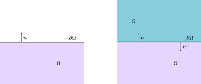
Figure 1: Diagram of the boundary and interface of a relaxed micromorphic continuum: (left) boundary with free surface, and (right) interface between two different relaxed micromorphic continua.

According to the Principle of Virtual Work, we can state that the the displacement field $u$ and the micro-distortion field $P$ have to satisfy the equality

$$\int_{0}^{T}\mathcal{W}^{\text{int}}=\int_{0}^{T}\mathcal{W}^{\rm ext}\,,$$ (10)

which implies the following duality condition to hold at a free relaxed micromorphic interface

$$\iint\limits_{\partial\Omega\times\left[0,T\right]}\langle t,\delta u\rangle=\iint\limits_{\partial\Omega\times\left[0,T\right]}\langle f^{\rm ext},\delta u\rangle\,,\qquad\iint\limits_{\partial\Omega\times\left[0,T\right]}\langle\tau,\delta P\rangle=\iint\limits_{\partial\Omega\times\left[0,T\right]}\langle\Phi^{\rm ext},\delta P\rangle\,,$$ (11)

where the generalized traction $t$ and the double traction $\tau$ are defined as

$$t=\left(\widetilde{\sigma}+\widehat{\sigma}\right)\,n\,,\qquad\qquad\qquad\tau=m\times n\,,$$ (12)

while $n$ is the normal at the boundary $\partial\Omega$, and the cross product acts row-wise. It is also recalled the expression of the traction for a classical Cauchy material

$$t_{\rm Cauchy}=\sigma_{\rm Cauchy}n\,,$$ (13)

where $\sigma_{\rm Cauchy}=\lambda\,\text{tr}\left(\text{sym}\nabla u\right)\,\mathbb{1}+2\mu\,\text{sym}\nabla u$ is the stress tensor for an isotropic linear elastic constitutive model.

The interface conditions between two relaxed micromorphic domains $\Omega^{-}$ and $\Omega^{+}$ can be similarly derived (see Fig. 1) and, in their strong form, they read

$$\begin{cases}t^{+}=t^{-}\,,\\ u^{+}=u^{-}\,,\end{cases}\qquad\qquad\qquad\begin{cases}\tau^{+}=\tau^{-}\,,\\ \left(P\times n\right)^{+}=\left(P\times n\right)^{-}\,.\end{cases}$$ (14)

As a particular case, if $\Omega^{+}$ is a classical Cauchy continuum, then the interface conditions reduce just to

$$\begin{cases}t_{\rm Cauchy}^{+}=t^{-}\,,\\ u^{+}=u^{-}\,,\end{cases}\qquad\qquad\quad\begin{cases}\tau=0\,,\\ \text{or}\\ \left(P\times n\right)=0\,.\end{cases}\hskip 34.14322pt$$ (15)

Since in a classical Cauchy material neither $m$ nor $P$ are defined, from the perspective of the higher order interface conditions the problem reduces to a free-end boundary conditions case. Therefore we can either chose the Neumann boundary conditions $\tau=0$, which can be interpreted as a “free microstructure” condition, or the Dirichlet boundary conditions $\left(P\times n\right)=0$, which can be interpreted as a “fixed microstructure” condition.

In the reminder of the paper we will set the curvature terms to zero ($\mathbb{L}_{\rm s}=\mathbb{L}_{\rm a}=\mathbb{M}_{\rm s}=\mathbb{M}_{\rm a}=0$ in eq.(2)), since their effect is most relevant in statics than in dynamics [52, 53]. It follows that neither the boundary conditions on $\tau$ nor the one on $P$ must be assigned in this particular case.

2.3 Numerical results

We perform a time harmonic study to analyze the response of finite size metamaterials using both fully microstructured and relaxed micromorphic models. An incident plane wave $u^{\rm I}$ travels in the domain $\Omega_{\rm C}^{1}$ and acts on the single and double shield devices of Fig. 3. The shields are made up of metamaterials, which themselves are made of unit cells of the type shown in Fig. 4. For the single-shield configuration, the size of the unit cell is $L_{\rm c}=2.5\ \rm mm$, this size corresponds to a scaling factor $s_{\rm F}=2.5$. On the double-shield, the metamaterial of the outer shield has $s_{\rm F}=1$ while the inner shield has $s_{\rm F}=2.5$. The properties of the material composing the matrix of the unit cell are reported in Fig. 4.

The dispersion curves of the two unit cells are presented together in Fig. 2. It can be seen the widening of the band-gap effect due to the two unit cell’s sizes. The parameters of the relaxed micromorphic model for the unit cell with $s_{\rm F}=1$ (see also [52]) and $s_{\rm F}=2.5$ can be found in Table 1. To obtain the parameters for the unit cell with $s_{\rm F}=2.5$ form the ones of the unit cell with $s_{\rm F}=1$, it is just necessary to scale $L_{\rm c}$ with the same factor of the size of the unit cell in eq.(3)-(4) (for more details see [57, 18]).

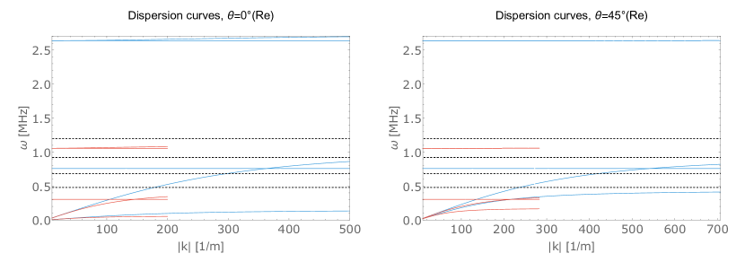
Figure 2: Dispersion curves of the metamaterials issued by the unit cell with $s_{\rm F}=2.5$ in red and with $s_{\rm F}=1$ in blue. The dashed lines represent the frequencies $\{0.48,0.68,0.92,1.2\}$ MHz that have been used for the simulations presented in the following sections.

$\lambda_{\text{e}}$ [GPa]	$\mu_{\text{e}}$ [GPa]	$\mu^{*}_{\text{e}}$ [GPa]	$\mu_{\text{c}}$ [GPa]
$2.33$	$10.92$	$0.67$	$2.28\times 10^{-3}$
$\lambda_{\rm m}$ [GPa]	$\mu_{\rm m}$ [GPa]	$\mu^{*}_{\rm m}$ [GPa]	$\rho$ [kg/m3]
$5.27$	$12.8$	$8.33$	$1485$
$\eta_{1}$ [kg/m]	$\eta_{2}$ [kg/m]	$\eta_{3}$ [kg/m]	$\eta^{*}_{1}$ [kg/m]
$8.60\times 10^{-5}$	$10^{-7}$	$-2.20\times 10^{-5}$	$3.30\times 10^{-5}$
$\overline{\eta}_{1}$ [kg/m]	$\overline{\eta}_{2}$ [kg/m]	$\overline{\eta}_{3}$ [kg/m]	$\overline{\eta}^{*}_{1}$ [kg/m]
$5.60\times 10^{-5}$	$7.30\times 10^{-4}$	$1.70\times 10^{-4}$	$9\times 10^{-7}$

$\lambda_{\text{e}}$ [GPa]	$\mu_{\text{e}}$ [GPa]	$\mu^{*}_{\text{e}}$ [GPa]	$\mu_{\text{c}}$ [GPa]
$2.33$	$10.92$	$0.67$	$2.28\times 10^{-3}$
$\lambda_{\rm m}$ [GPa]	$\mu_{\rm m}$ [GPa]	$\mu^{*}_{\rm m}$ [GPa]	$\rho$ [kg/m3]
$5.27$	$12.8$	$8.33$	$1485$
$\eta_{1}$ [kg/m]	$\eta_{2}$ [kg/m]	$\eta_{3}$ [kg/m]	$\eta^{*}_{1}$ [kg/m]
$5.38\times 10^{-4}$	$6.25\times 10^{-7}$	$-1.38\times 10^{-4}$	$2.06\times 10^{-4}$
$\overline{\eta}_{1}$ [kg/m]	$\overline{\eta}_{2}$ [kg/m]	$\overline{\eta}_{3}$ [kg/m]	$\overline{\eta}^{*}_{1}$ [kg/m]
$3.50\times 10^{-4}$	$4.56\times 10^{-3}$	$1.06\times 10^{-3}$	$5.63\times 10^{-6}$

Table 1: Parameters of the relaxed micromorphic model for the unit cell of Fig. 4 when (left) $L_{\rm c}=1$ mm and (right) $L_{\rm c}=2.5$ mm. It is highlighted that in order to obtain the parameters for the unit cell that is just homothetically scaled by a factor $s_{\rm F}=2.5$ it is enough to change the value of $L_{\rm c}$ form 1 to 2.5 mm in the expressions reported in equation (3)-(4) (see also [57, 18])

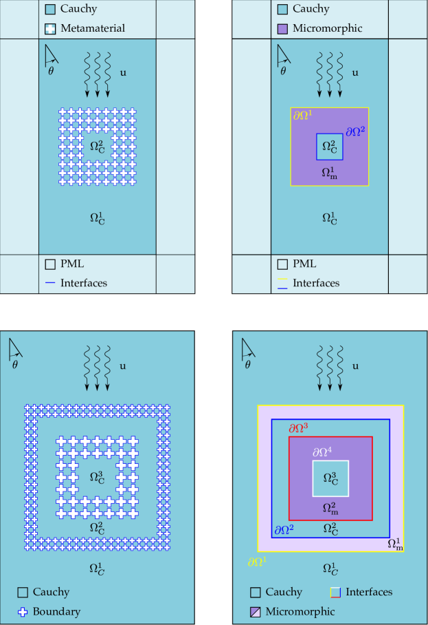
Figure 3: Schematics of metamaterials’ shields: (top) single shield and (bottom) double shield. In the latter, the perfectly matched layer surrounding the outermost Cauchy continuum is still present but it is here omitted for better depiction of the details of the double-shield’s configuration.

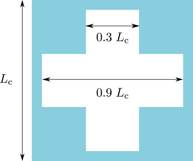
$L_{\rm c}$	$\rho_{\rm Al}$	$\lambda_{\rm Al}$	$\mu_{\rm Al}$
[mm]	[kg/m3]	[GPa]	[GPa]
1	2700	5.11	2.63

Figure 4: (left panel) unit cell geometry; (right panel) material and geometrical properties of the aluminum unit cell: size of the unit cell $L_{\rm c}$, density $\rho_{\rm Al}$, and the Lamé constants $\lambda_{\rm Al}$ and $\mu_{\rm Al}$.

All the numerical studies are performed under the plane strain hypothesis. The incident wave $u^{\rm I}$ travels in the external Cauchy continuum and can be defined either as a pressure $P$ or a shear $S$ wave as

$$u^{\rm I}=a\,\psi^{\rm P/S,I}\,e^{i\left(k_{1}^{\rm P/S,I}\,x_{1}+k_{2}^{\rm P/S,I}\,x_{2}-\omega\,t\right)}\,,\quad\text{with}\quad\left\{\begin{array}[]{ll}k_{1}^{\rm P,I}=\sqrt{\dfrac{\rho_{\rm Al}}{\lambda_{\rm Al}+2\mu_{\rm Al}}\omega^{2}-\left(k_{2}^{\rm P,I}\right)^{2}}\\[14.22636pt] k_{1}^{\rm S,I}=\sqrt{\dfrac{\rho_{\rm Al}}{\mu_{\rm Al}}\omega^{2}-\left(k_{2}^{\rm S,I}\right)^{2}}\end{array}\right.\,,$$ (18)

where $a$ is the amplitude, $\psi^{\rm P/S,I}$ is the normalized eigenvector associated with the pressure or shear wave, $k_{1}^{\rm P/S,I}$ and $k_{2}^{\rm P/S,I}$ are the components of the wave vector, and $\omega$ is the frequency.

The perfect contact condition at each interface between the relaxed micromorphic continuum and the classical Cauchy continuum (see Fig. 3) are reported in eq.(15). For the unit cell considered in this work, in the dynamic range studied, the curvature terms have a negligible effect in the metamaterial’s response [15, 52]. This allows for setting $\mathbb{L}_{\rm s}=\mathbb{L}_{\rm a}=\mathbb{M}_{\rm s}=\mathbb{M}_{\rm a}=0$, thus the curvature terms vanish and no double traction has to be defined on the boundaries and the interface conditions reduce to just eq.(15)₁.

Let us consider the equilibrium conditions derived from eq.(15) as they act, for example, on the boundary $\partial\Omega^{1}$. The superposition principle allows for the decomposition of the displacement and traction on the Cauchy side, into an incident and scattered component. The scattered components are indicated by the subscript “sca”, and the superscripts refer to their domain. The traction $t^{\rm I}$ is that produced by the incident wave and the conditions can be summarized as

$$\left\{\begin{array}[]{ccccccccccccc}u^{-}&=&u^{+}&\quad\Longleftrightarrow&\quad u^{\Omega_{\rm m}^{1}}&=&u^{\Omega_{\rm C}^{1}}_{\rm sca}+u^{\rm I}\\[5.69054pt] t^{-}&=&t^{+}&\quad\Longleftrightarrow&\quad t^{\Omega_{\rm\rm m}^{1}}&=&t^{\Omega_{\rm C}^{1}}_{\rm sca}+t^{\rm I}\end{array}\right.\quad\mathrm{on}\quad\partial\Omega^{1}\,.$$ (21)

As a consequence, on the boundary $\partial\Omega_{\rm C}^{1}$, we can then prescribe

$$u^{\Omega_{\rm C}^{1}}_{\mathrm{sca}}=u^{\Omega_{\rm m}^{1}}-u^{\rm I}\,,$$ (22)

and the associated tractions $t^{\Omega_{\rm C}^{1}}_{\mathrm{sca}}$ and $t^{\Omega_{\rm m}^{1}}$ derive from the solution of the correspondent displacement fields. Furthermore, on the boundary, the tractions of $\Omega_{\rm C}^{1}$ differ with respect to the tractions $\Omega_{\rm m}^{1}$ by

$$t^{\Omega_{\rm C}^{1}}_{\mathrm{sca}}-t^{\Omega_{\rm m}^{1}}=-t^{\rm I}\ .$$ (23)

Thus we must prescribe $-t^{\rm I}$ on the boundary $\partial\Omega^{1}$ of $\Omega_{\rm C}^{1}$ to ensure the continuity of tractions reported in eq.(21). For the microstructured material, it is sufficient to prescribe $-t^{\rm I}$ on the free boundary of the holes. Analogous conditions apply to the other boundaries.

3 Parametric study on the thickness of a shielding device: capability limit for the relaxed micromorphic model

In this section, we present the results of a simple shield device modeled both with a full-microstructure model and with the relaxed micromorphic model. The displacement in the subsequent figures is normalized by the amplitude of the incident wave. In Fig. 5, we can see that a shield device made up of only one unit cell is not able to ensure the desired shielding effect, and this is true both for the microstructured and the relaxed micromorphic models.

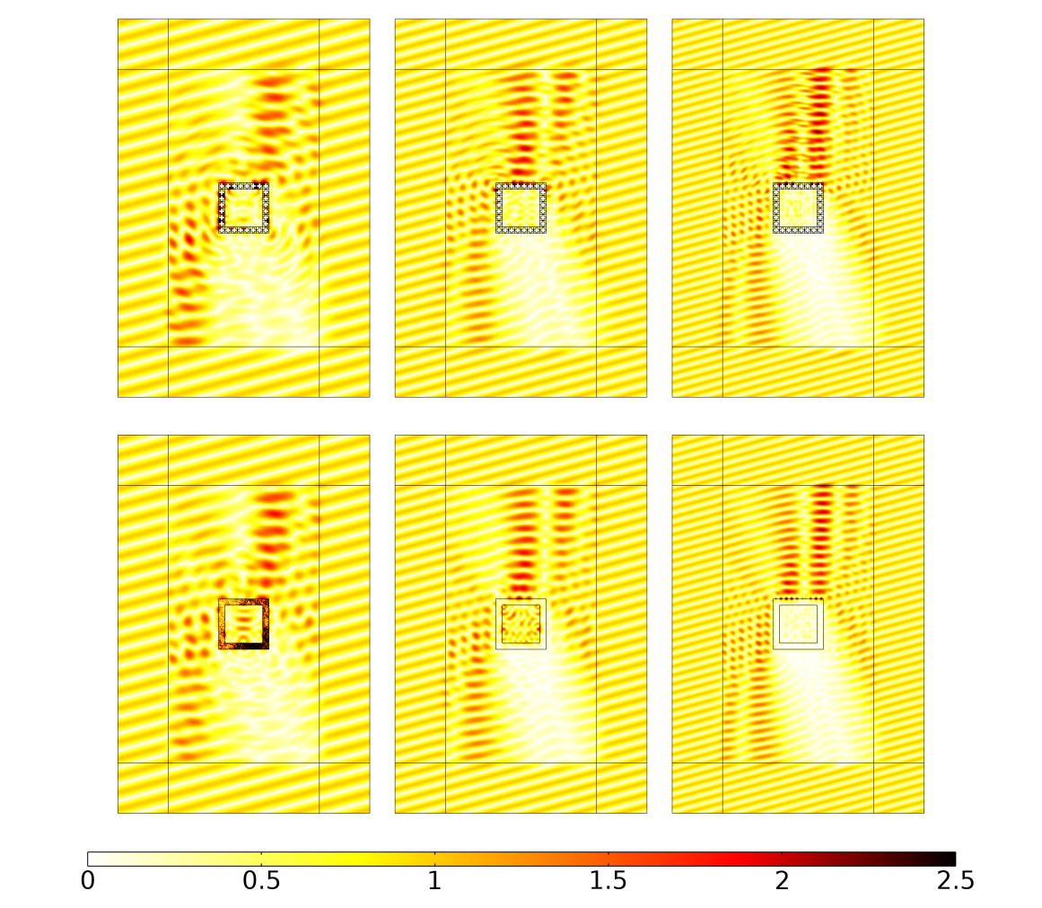
Figure 5: Real part of the normalized displacement field of the microstructured material and its equivalent micromorphic continuum for a shield of 1 unit cell thick, for an incident angle $\phi=15^{\circ}$: (first row) microstructured material and (second row) equivalent micromorphic model for $\omega=0.48$ MHz, $\omega=0.68$ MHz, and $\omega=0.92$ MHz. All frequencies fall in the band-gap range of the considered metamaterial.

We remark that the reflection pattern is nevertheless well captured by the relaxed micromorphic model, even if the shield’s thickness is of only one unit cell, while the displacement pattern inside the shield shows a loss of accuracy. This is due to the fact that the relaxed micromorphic model, being a homogenized model, needs a certain domain size to guarantee results with a high level of accuracy, and we show this by performing a parametric study on the shield’s thickness (see Fig. 5-9).

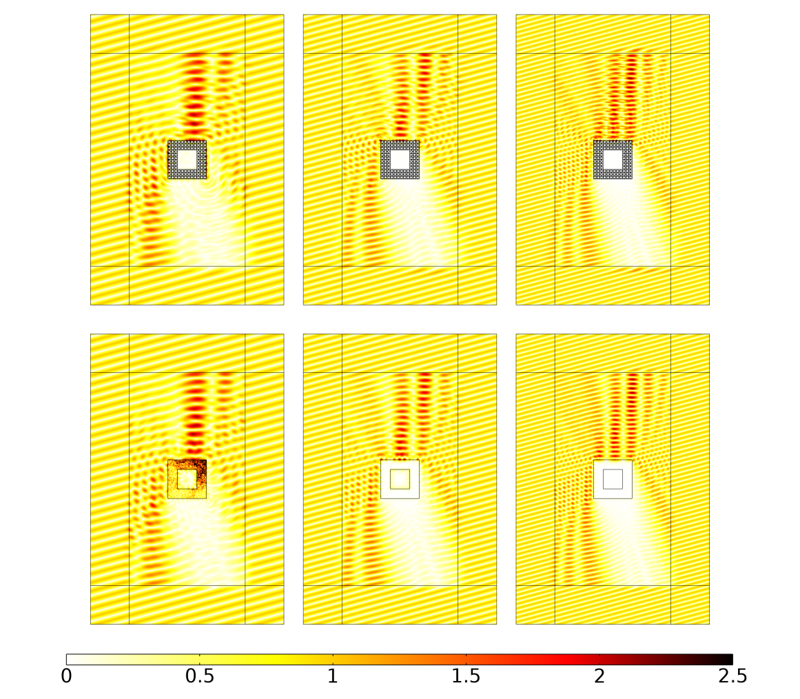
Figure 6: Real part of the normalized displacement field of the microstructured material and its equivalent micromorphic continuum for a shield of 3 unit cells thick, for an incident angle $\phi=15^{\circ}$: (first row) microstructured material and (second row) equivalent micromorphic model for $\omega=0.48$ MHz, $\omega=0.68$ MHz, and $\omega=0.92$ MHz. All frequencies fall in the band-gap region of the considered metamaterial.

We can infer from Fig. 6-9 that both the outer and inner displacement fields are well reproduced by the relaxed micromorphic model, as early as the shield is thick enough. Indeed, we established that both the shielding effect and the relaxed micromorphic model accuracy can be considered to be satisfactory already with a 3 unit cell thickness, especially when considering frequencies in the band-gap range.

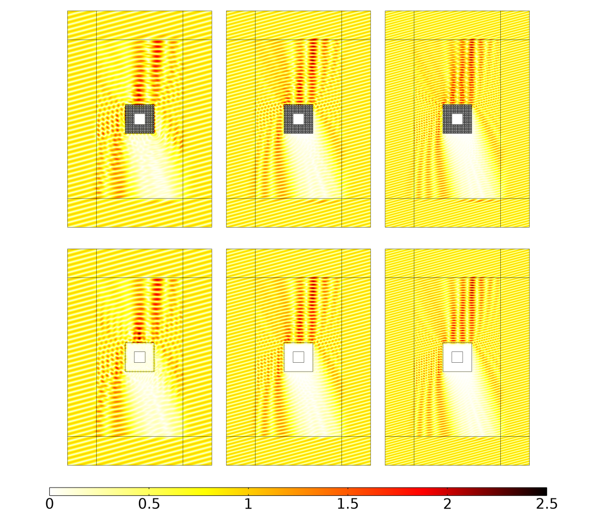
Figure 7: Real part of the normalized displacement field of the microstructured material and its equivalent micromorphic continuum for a shield of 5 unit cells thick, for an incident angle $\phi=15^{\circ}$: (first row) microstructured material and (second row) equivalent micromorphic model for $\omega=0.48$ MHz, $\omega=0.68$ MHz, and $\omega=0.92$ MHz. All frequencies fall in the band-gap region of the considered metamaterial.

All the simulations performed in this section and in the following ones have been run on 2$\times$AMD EPYC 7453 28-Core Processor. We observe faster computing times for the relaxed micromorphic model than for the full-microstructure simulations, more details are presented in the following sections.

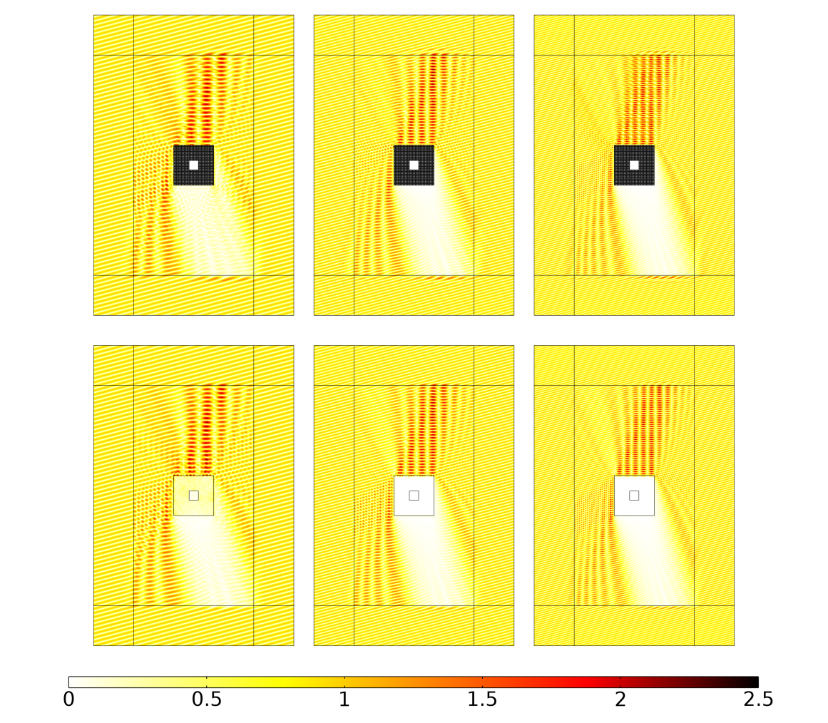
Figure 8: Real part of the normalized displacement field of the microstructured material and its equivalent micromorphic continuum for a shield of 10 unit cells thick, for an incident angle $\phi=15^{\circ}$: (first row) microstructured material and (second row) equivalent micromorphic model for $\omega=0.48$ MHz, $\omega=0.68$ MHz, and $\omega=0.92$ MHz. All frequencies fall in the band-gap region of the considered metamaterial.

For the sake of completeness, we also present in Fig. 8 the reflection pattern of a simple shield device which is 3 unit cells thick and for a 0^∘ angle of incidence. Analogous results can be obtained for all other angles of incidence, showing the effectiveness of the relaxed micromorphic model to unveil the macroscopic metamaterial’s anisotropy.

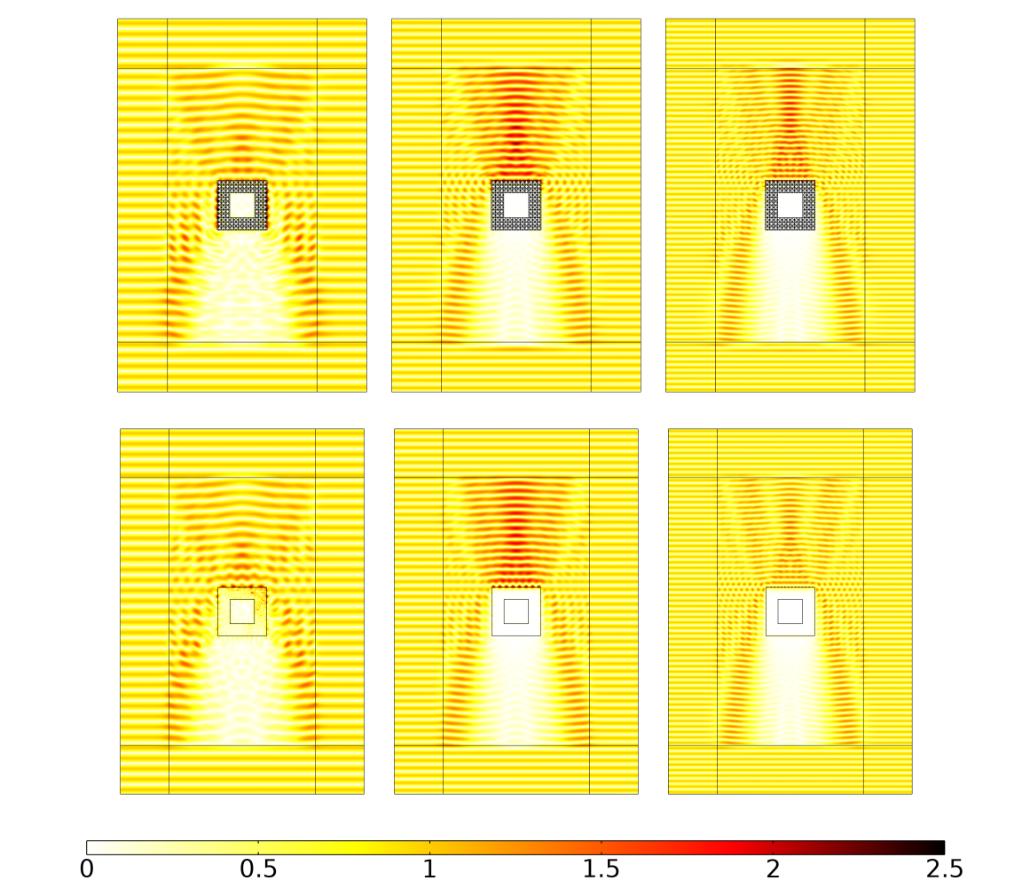
Figure 9: Real part of the normalized displacement field of the microstructured material and its equivalent micromorphic continuum for a shield of 3 unit cells thick, for an incident angle $\phi=0^{\circ}$: (first row) microstructured material and (second row) equivalent micromorphic model for $\omega=0.48$ MHz, $\omega=0.68$ MHz, and $\omega=0.92$ MHz. All frequencies fall in the band-gap region of the considered metamaterial.

4 Design of a double shield device

In this section, we start exploring multi-shield devices with the aim of increasing the frequency range for which the inner core of the structure is protected from an external excitation. To do so, we use two different sizes of the unit cell presented in Fig. 4 with ${\rm s_{F}}=1$ for the outer and ${\rm s_{F}}=2.5$ for the inner shield. In this way the inner structure’s core will be protected in the overlapping intervals [1.11,2.65] MHz and [0.44,1.06] MHz.

We show in Fig. 10 a first multi-shield device composed of 3 unit cells for the outer shield and 1 unit cell for the inner shield: the scattering behavior is given for an incidence angle of $15^{\circ}$ and for a frequency of $\omega=0.92$ MHz, which falls in the band-gap of the outer shield. We see that the relaxed micromorphic model recovers well the scattering pattern of the double-shield device at a fraction of the computational cost and with lower memory use. The simulation that uses the relaxed micromorphic model takes 61 s in contrast to the 156 s needed by the geometrically detailed simulation. The gain in computational time, which is already visible for these simple structures, will be more significant when studying larger structures, as those presented in Sect. 5.

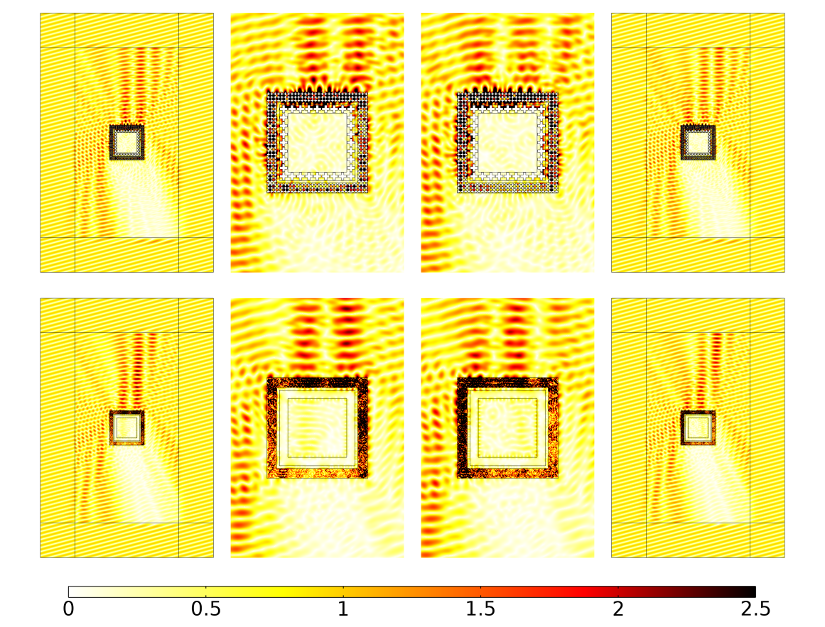
Figure 10: Imaginary (first two columns) and real (last two columns) part of the normalized displacement field of the microstructured material and its equivalent micromorphic continuum: (first row) microstructured material and (second row) equivalent micromorphic model for $\omega=0.92$ MHz. The thickness of the outer shield is 3 unit cells, and the thickness of the inner shield is 1 unit cell.

In Fig. 11 we show the same results for a multi-shield device made of two 3x3 cell shields. The results are again convincing, at a fraction of the computational cost.

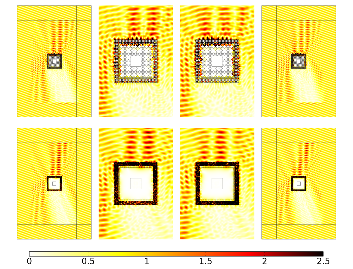
Figure 11: Imaginary (first two columns) and real (last two columns) part of the normalized displacement field of the microstructured material and its equivalent micromorphic continuum: (first row) microstructured material and (second row) equivalent micromorphic model for $\omega=0.92$ MHz. The thickness of the outer shield is 3 unit cells, and the thickness of the inner shield is 3 unit cells.

Similar results can be shown for other angles of incidence. In order to complete our exploration, we now choose a frequency $\omega=1.2$ MHz which falls in the band-gap of the inner shield metamaterial. Fig. 12 shows the structure’s response for $\omega=1.2$ MHz and an angle of incidence of $0^{\circ}$. Once again, the relaxed micromorphic model performs really well at a fraction of the computational cost when reproducing the displacement field of the outer Cauchy domain. In this case, the solution of the relaxed micromorphic model takes 94 s when the full-microstructure simulation needs 178 s.

However, these results also showcase a limitation of the micromorphic type models when the curves above the band gap grow flat, as is the case for the unit cell used in this work, see Fig. 2. In Fig. 12, the inner shield does not properly capture the excitation modes at $\omega=1.2$ MHz, and overall there is a slight inaccuracy in the prediction of the interior displacement field as opposed to the displacement present in the full-microstructure simulation. More particularly, the relaxed micromorphic model predicts a complete screening while the microstructured simulations show a small displacement occurring in the interior part. This difference is due, to a big extent, to the fact that we are considering only the first 6 modes for the relaxed micromorphic model, while at the considered frequency higher order modes can be slightly activated.

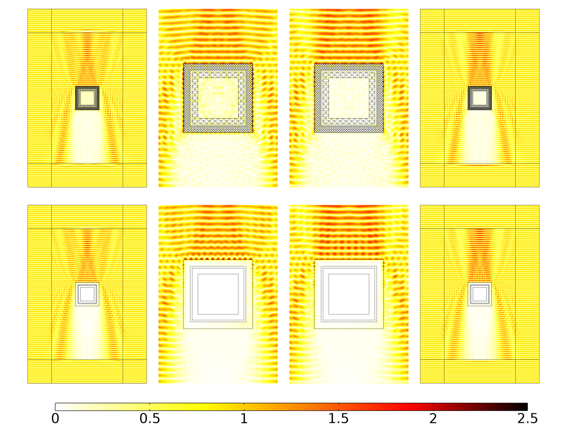
Figure 12: Imaginary (first two columns) and real (last two columns) part of the normalized displacement field of the microstructured material and its equivalent micromorphic continuum: (first row) microstructured material and (second row) equivalent micromorphic model for $\omega=1.2$ MHz. The thickness of the outer shield is 3 unit cells, and the thickness of the inner shield is 1 unit cell.

5 Multiple-shields Optimization

While metamaterials’ modeling has gathered a wealth of research effort in the last decades, the study of large-scale metamaterial’s structures consisting of many metamaterials’ components has received little attention. For example, many researchers have successfully proposed metamaterials’ shielding configurations [1, 39, 40, 49], but no effort is paid to the study of the global reflection pattern of a system consisting of multiple shielding devices. This lack is mainly due to the computational limitations of full-microstructure simulations, on the one hand, and to lack of knowledge of homogenized approaches on well-posed boundary conditions, on the other.

Thanks to the relaxed micromorphic model presented so far, with the associated well-posed boundary conditions, we are now able to explore large-scale optimization problems of this type. The results of Sect. 3 and 4 show an additional region with no displacement on the opposite side of the boundary of the shield that is first impacted by the incident wave. We now explore a multiple-shields structure in order to investigate the displacement field in the region situated between and behind a group of single shields. Fig. 13 shows the global reflection pattern of the multiple-shields systems. It is apparent that the configurations chosen are effective for local shielding of the internal small squares, as well as for the global shielding between the simple shields, as far as a 0^∘ incidence is considered. For other angles of incidence the global shielding effect clearly loses its effectiveness. To optimize the global shielding effect an additional “metamaterial’s ring” can be added to the configuration of Fig. 14 and the local and global reflection patterns can be explored for different angles of incidence. Such explorations would not be possible, or very time consuming, with simulations with the full-microstructure. The simulation of Fig. 14 of the relaxed micromorphic model needed 35 min 8 s, while that of the microstructured case required 2 h 11 min 46 s. The computational gain clearly grows fast as soon as larger structures are investigated.

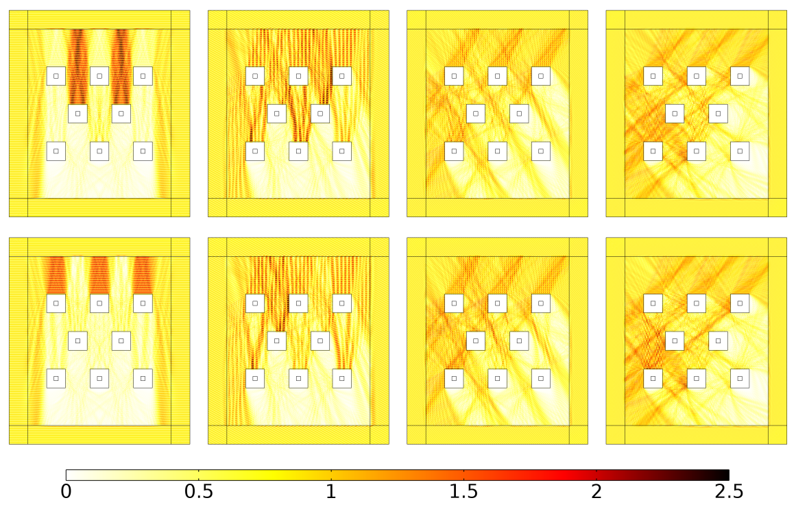
Figure 13: Normalized displacement field of a multiple shield structure for an incident wave of frequency $\omega=0.92$ MHz: (first row) imaginary and (second row) real part of the displacement. Form left to right the angle of the incident wave is $\phi=0^{\circ}$, $\phi=15^{\circ}$, $\phi=30^{\circ}$, and $\phi=45^{\circ}$. The thickness of each single shields is 10 unit cells.

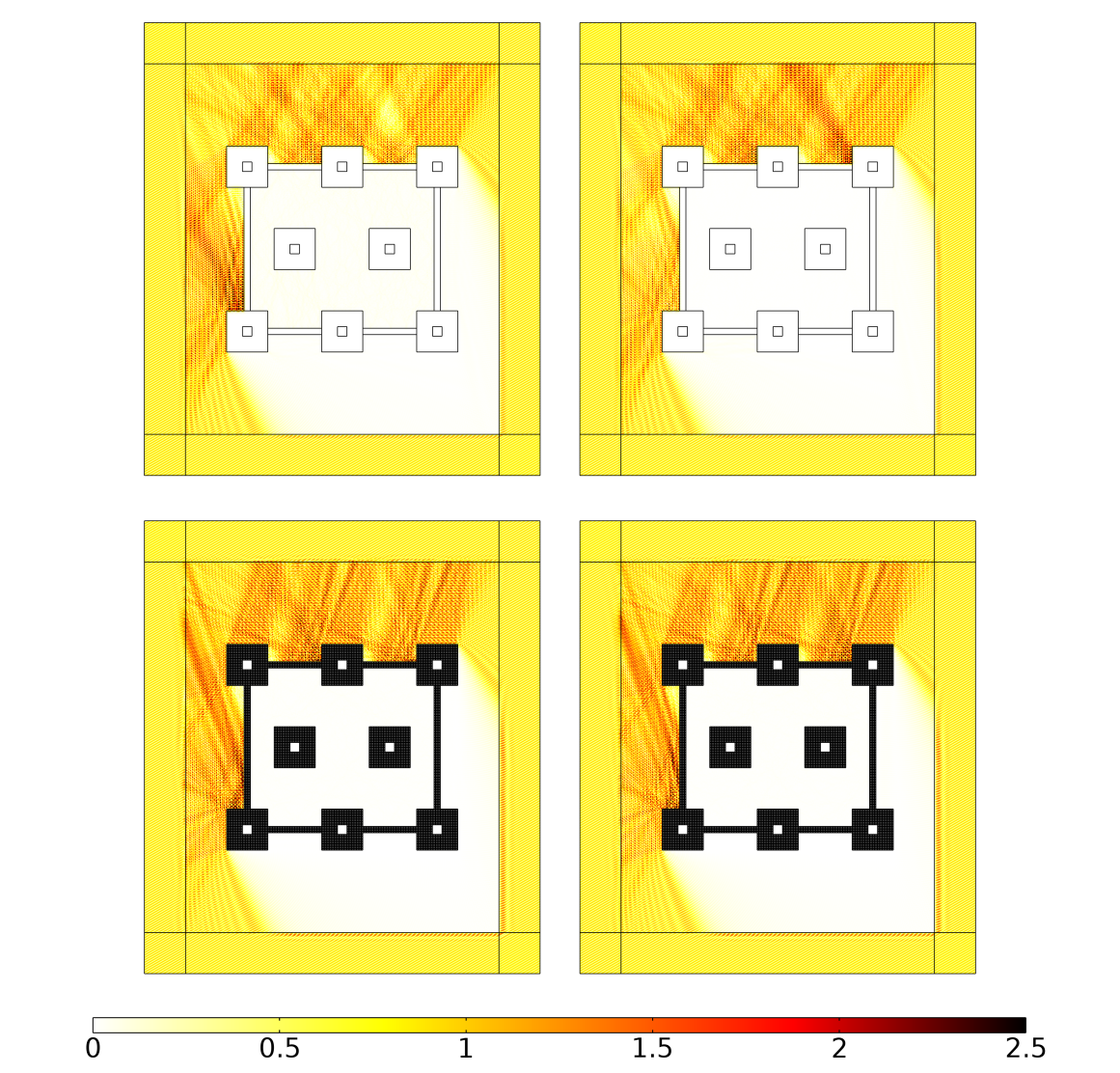
Figure 14: Peripheral shield 4 unit cells thick for an incident wave with a frequency of $\omega=0.92$ MHz and an angle of $\phi=30^{\circ}$. Real (left) and imaginary (right) part of the normalized displacement for the (first row) microstructured material and (second row) equivalent micromorphic continuum. The thickness of each single shields is 10 unit cells.

6 Conclusions

In this paper, we showed that the relaxed micromorphic model can be effectively used to describe wave propagation and scattering in complex structures combining metamaterials’ and classical materials’ bricks of finite size. We successfully designed a double-shield device extending the frequency range for which the screening effect occurs, thanks to the use of unit cells with different size. We also designed a multiple-shield structure allowing to protect both the internal part of each shield and the external region between the shields. Thanks to the model’s simplification (homogenized model featuring few frequency-independent parameters), these designs were obtained at a fraction of the computational cost with respect to classical simulations based on Cauchy elasticity. This gain in computational time will be primordial for further works where more and more complex structures will be investigated with the aim of targeting real engineering applications. The results of the present paper open the way to more systematic explorations of engineering large-scale structures that can control elastic waves, thus creating favorable conditions for effective energy conversion and re-use.

Acknowledgements.

Angela Madeo, Leonardo A. Perez Ramirez, and Gianluca Rizzi acknowledge support from the European Commission through the funding of the ERC Consolidator Grant META-LEGO, N^∘ 101001759. The authors also gratefully acknowledge the computing time provided on the Linux HPC cluster at Technical University Dortmund (LiDO3), partially funded in the course of the Large-Scale Equipment Initiative by the German Research Foundation (DFG) as project 271512359.

References

- [1] Y Achaoui, T Antonakakis, S Brûlé, RV Craster, S Enoch and S Guenneau “Clamped seismic metamaterials: ultra-low frequency stop bands” In New Journal of Physics 19.6 IOP Publishing, 2017, pp. 063022
- [2] Alexios Aivaliotis, Domenico Tallarico, Marco-Valerio d’Agostino, Ali Daouadji, Patrizio Neff and Angela Madeo “Frequency-and angle-dependent scattering of a finite-sized meta-structure via the relaxed micromorphic model” In Archive of Applied Mechanics 90.5 Springer, 2020, pp. 1073–1096
- [3] Holm Altenbach, Joël Pouget, Martine Rousseau, Bernard Collet and Thomas Michelitsch “Generalized models and non-classical approaches in complex materials 2” Springer, 2018
- [4] Johannes Altenbach, Holm Altenbach and Victor A Eremeyev “On generalized Cosserat-type theories of plates and shells: a short review and bibliography” In Archive of Applied Mechanics 80.1 Springer, 2010, pp. 73–92
- [5] Emanuele Baravelli and Massimo Ruzzene “Internally resonating lattices for bandgap generation and low-frequency vibration control” In Journal of Sound and Vibration 332.25 Elsevier, 2013, pp. 6562–6579
- [6] Osama R Bilal, David Ballagi and Chiara Daraio “Architected lattices for simultaneous broadband attenuation of airborne sound and mechanical vibrations in all directions” In Physical Review Applied 10.5 APS, 2018, pp. 054060
- [7] G. Bordiga, L. Cabras, A. Piccolroaz and D. Bigoni “Prestress tuning of negative refraction and wave channeling from flexural sources” In Applied Physics Letters 114.4 AIP Publishing LLC, 2019, pp. 041901
- [8] Claude Boutin, Antoine Rallu and Stéphane Hans “Large scale modulation of high frequency waves in periodic elastic composites” In Journal of the Mechanics and Physics of Solids 70 Elsevier, 2014, pp. 362–381
- [9] Tiemo Bückmann, Muamer Kadic, Robert Schittny and Martin Wegener “Mechanical cloak design by direct lattice transformation” In Proceedings of the National Academy of Sciences 112.16 National Acad Sciences, 2015, pp. 4930–4934
- [10] Paolo Celli, Behrooz Yousefzadeh, Chiara Daraio and Stefano Gonella “Bandgap widening by disorder in rainbow metamaterials” In Applied Physics Letters 114.9 AIP Publishing LLC, 2019, pp. 091903
- [11] Wen Chen and Jacob Fish “A dispersive model for wave propagation in periodic heterogeneous media based on homogenization with multiple spatial and temporal scales” In J. Appl. Mech. 68.2, 2001, pp. 153–161
- [12] Alessandro Ciallella, Ivan Giorgio, Simon R Eugster, Nicola L Rizzi and Francesco Dell’Isola “Generalized beam model for the analysis of wave propagation with a symmetric pattern of deformation in planar pantographic sheets” In Wave Motion 113 Elsevier, 2022, pp. 102986
- [13] Richard V Craster, Julius Kaplunov and Aleksey V Pichugin “High-frequency homogenization for periodic media” In Proceedings of the Royal Society A: Mathematical, Physical and Engineering Sciences 466.2120 The Royal Society Publishing, 2010, pp. 2341–2362
- [14] Steven A Cummer, Johan Christensen and Andrea Alù “Controlling sound with acoustic metamaterials” In Nature Reviews Materials 1.3 Nature Publishing Group, 2016, pp. 1–13
- [15] Marco Valerio d’Agostino, Gabriele Barbagallo, Ionel-Dumitrel Ghiba, Bernhard Eidel, Patrizio Neff and Angela Madeo “Effective description of anisotropic wave dispersion in mechanical band-gap metamaterials via the relaxed micromorphic model” In Journal of elasticity 139.2 Springer, 2020, pp. 299–329
- [16] Francesco Dell’Isola, Ivan Giorgio and Ugo Andreaus “Elastic pantographic 2D lattices: a numerical analysis on the static response and wave propagation” In Proceedings of the Estonian Academy of Sciences 64.3 Teaduste Akadeemia Kirjastus (Estonian Academy Publishers), 2015, pp. 219
- [17] Francesco Dell’Isola, Angela Madeo and Luca Placidi “Linear plane wave propagation and normal transmission and reflection at discontinuity surfaces in second gradient 3D continua” In ZAMM-Journal of Applied Mathematics and Mechanics/Zeitschrift für Angewandte Mathematik und Mechanik 92.1 Wiley Online Library, 2012, pp. 52–71
- [18] F. Demore, G. Rizzi, M. Collet, P. Neff and A. Madeo “Unfolding engineering metamaterials design: Relaxed micromorphic modeling of large-scale acoustic meta-structures” In Journal of the Mechanics and Physics of Solids 168, 2022, pp. 104995
- [19] M.G. El Sherbiny and L. Placidi “Discrete and continuous aspects of some metamaterial elastic structures with band gaps” In Archive of Applied Mechanics 88.10 Springer, 2018, pp. 1725–1742
- [20] Daniel P Elford, Luke Chalmers, Feodor V Kusmartsev and Gerry M Swallowe “Matryoshka locally resonant sonic crystal” In The Journal of the Acoustical Society of America 130.5 Acoustical Society of America, 2011, pp. 2746–2755
- [21] Victor Eremeyev and Holm Altenbach “Basics of mechanics of micropolar shells” In Shell-like structures Springer, 2017, pp. 63–111
- [22] Victor A Eremeyev “Two-and three-dimensional elastic networks with rigid junctions: modeling within the theory of micropolar shells and solids” In Acta Mechanica 230.11 Springer, 2019, pp. 3875–3887
- [23] Victor A Eremeyev, Faris Saeed Alzahrani, Antonio Cazzani, Tasawar Hayat, Emilio Turco and Violetta Konopińska-Zmysłowska “On existence and uniqueness of weak solutions for linear pantographic beam lattices models” In Continuum Mechanics and Thermodynamics 31.6 Springer, 2019, pp. 1843–1861
- [24] Victor A Eremeyev, Claude Boutin and David Steigmann “Linear pantographic sheets: existence and uniqueness of weak solutions” In Journal of Elasticity 132.2 Springer, 2018, pp. 175–196
- [25] A Cemal Eringen “Mechanics of micromorphic continua” In Mechanics of generalized continua Springer, 1968, pp. 18–35
- [26] Tobias Frenzel, Muamer Kadic and Martin Wegener “Three-dimensional mechanical metamaterials with a twist” In Science 358.6366 American Association for the Advancement of Science, 2017, pp. 1072–1074
- [27] Ionel-Dumitrel Ghiba, Patrizio Neff, Angela Madeo, Luca Placidi and Giuseppe Rosi “The relaxed linear micromorphic continuum: existence, uniqueness and continuous dependence in dynamics” In Mathematics and Mechanics of Solids 20.10 SAGE Publications Sage UK: London, England, 2015, pp. 1171–1197
- [28] H. Goh and L.F. Kallivokas “Inverse metamaterial design for controlling band gaps in scalar wave problems” In Wave Motion 88 Elsevier, 2019, pp. 85–105
- [29] Sébastien Guenneau, Alexander Movchan, Gunnar Pétursson and S Anantha Ramakrishna “Acoustic metamaterials for sound focusing and confinement” In New Journal of physics 9.11 IOP Publishing, 2007, pp. 399
- [30] Nadège Kaina, Alexandre Causier, Yoan Bourlier, Mathias Fink, Thomas Berthelot and Geoffroy Lerosey “Slow waves in locally resonant metamaterials line defect waveguides” In Scientific reports 7.1 Nature Publishing Group, 2017, pp. 1–11
- [31] P.I. Koutsianitis, G.K. Tairidis, G.A. Drosopoulos and G.E. Stavroulakis “Conventional and star-shaped auxetic materials for the creation of band gaps” In Archive of Applied Mechanics 89.12 Springer, 2019, pp. 2545–2562
- [32] Anastasiia O Krushynska, Marco Miniaci, Federico Bosia and Nicola M Pugno “Coupling local resonance with Bragg band gaps in single-phase mechanical metamaterials” In Extreme Mechanics Letters 12 Elsevier, 2017, pp. 30–36
- [33] Roderic Lakes “Foam structures with a negative Poisson’s ratio” In Science 235.4792 American Association for the Advancement of Science, 1987, pp. 1038–1040
- [34] Zhengyou Liu, Xixiang Zhang, Yiwei Mao, YY Zhu, Zhiyu Yang, Che Ting Chan and Ping Sheng “Locally resonant sonic materials” In science 289.5485 American Association for the Advancement of Science, 2000, pp. 1734–1736
- [35] Ben Lustig, Guy Elbaz, Alan Muhafra and Gal Shmuel “Anomalous energy transport in laminates with exceptional points” In Journal of the Mechanics and Physics of Solids 133 Elsevier, 2019, pp. 103719
- [36] Angela Madeo, Patrizio Neff, Ionel-Dumitrel Ghiba, Luca Placidi and Giuseppe Rosi “Wave propagation in relaxed micromorphic continua: modeling metamaterials with frequency band-gaps” In Continuum Mechanics and Thermodynamics 27.4 Springer, 2015, pp. 551–570
- [37] Raymond David Mindlin “Microstructure in linear elasticity”, 1963
- [38] M. Miniaci, R.K. Pal, R. Manna and M. Ruzzene “Valley-based splitting of topologically protected helical waves in elastic plates” In Physical Review B 100.2 APS, 2019, pp. 024304
- [39] Marco Miniaci, Nesrine Kherraz, Charles Cröenne, Matteo Mazzotti, Maryam Morvaridi, Antonio S Gliozzi, Miguel Onorato, Federico Bosia and Nicola Maria Pugno “Hierarchical large-scale elastic metamaterials for passive seismic wave mitigation” In EPJ Applied Metamaterials 8 EDP Sciences, 2021, pp. 14
- [40] Marco Miniaci, Anastasiia Krushynska, Federico Bosia and Nicola M Pugno “Large scale mechanical metamaterials as seismic shields” In New Journal of Physics 18.8 IOP Publishing, 2016, pp. 083041
- [41] D. Misseroni, A.B. Movchan and D. Bigoni “Omnidirectional flexural invisibility of multiple interacting voids in vibrating elastic plates” In Proceedings of the Royal Society A 475.2229 The Royal Society Publishing, 2019, pp. 20190283
- [42] Diego Misseroni, Daniel J Colquitt, Alexander B Movchan, Natasha V Movchan and Ian Samuel Jones “Cymatics for the cloaking of flexural vibrations in a structured plate” In Scientific reports 6.1 Nature Publishing Group, 2016, pp. 1–11
- [43] Lorenzo Morini, Yoann Eyzat and Massimiliano Gei “Negative refraction in quasicrystalline multilayered metamaterials” In Journal of the Mechanics and Physics of Solids 124 Elsevier, 2019, pp. 282–298
- [44] Lidiia Nazarenko, Rainer Glüge and Holm Altenbach “On variational principles in coupled strain-gradient elasticity” In Mathematics and Mechanics of Solids SAGE Publications Sage UK: London, England, 2022, pp. 10812865221081854
- [45] Patrizio Neff, Bernhard Eidel, Marco Valerio d’Agostino and Angela Madeo “Identification of scale-independent material parameters in the relaxed micromorphic model through model-adapted first order homogenization” In Journal of Elasticity 139.2 Springer, 2020, pp. 269–298
- [46] Patrizio Neff, Ionel-Dumitrel Ghiba, Markus Lazar and Angela Madeo “The relaxed linear micromorphic continuum: well-posedness of the static problem and relations to the gauge theory of dislocations” In Quarterly Journal of Mechanics and Applied Mathematics 68.1 OUP, 2015, pp. 53–84
- [47] Patrizio Neff, Ionel-Dumitrel Ghiba, Angela Madeo, Luca Placidi and Giuseppe Rosi “A unifying perspective: the relaxed linear micromorphic continuum” In Continuum Mechanics and Thermodynamics 26.5 Springer, 2014, pp. 639–681
- [48] A.N. Norris, F.A. Amirkulova and W.J. Parnell “Active elastodynamic cloaking” In Mathematics and Mechanics of Solids 19.6 Sage Publications Sage UK: London, England, 2014, pp. 603–625
- [49] Antonio Palermo, Sebastian Krödel, Alessandro Marzani and Chiara Daraio “Engineered metabarrier as shield from seismic surface waves” In Scientific reports 6.1 Nature Publishing Group, 2016, pp. 1–10
- [50] G Rizzi, F Dal Corso, D Veber and D Bigoni “Identification of second-gradient elastic materials from planar hexagonal lattices. Part I: Analytical derivation of equivalent constitutive tensors” In International Journal of Solids and Structures 176 Elsevier, 2019, pp. 1–18
- [51] G Rizzi, F Dal Corso, D Veber and D Bigoni “Identification of second-gradient elastic materials from planar hexagonal lattices. Part II: Mechanical characteristics and model validation” In International Journal of Solids and Structures 176 Elsevier, 2019, pp. 19–35
- [52] Gianluca Rizzi, Marco Valerio d’Agostino, Patrizio Neff and Angela Madeo “Boundary and interface conditions in the relaxed micromorphic model: Exploring finite-size metastructures for elastic wave control” In Mathematics and Mechanics of Solids 27.6 SAGE Publications Sage UK: London, England, 2022, pp. 1053–1068
- [53] Gianluca Rizzi, Patrizio Neff and Angela Madeo “Metamaterial shields for inner protection and outer tuning through a relaxed micromorphic approach” In Philosophical Transactions of the Royal Society A 380.2231 The Royal Society, 2022, pp. 20210400
- [54] Ashwin Sridhar, Varvara G Kouznetsova and Marc GD Geers “A general multiscale framework for the emergent effective elastodynamics of metamaterials” In Journal of the Mechanics and Physics of Solids 111 Elsevier, 2018, pp. 414–433
- [55] A. Srivastava “Metamaterial properties of periodic laminates” In Journal of the Mechanics and Physics of Solids 96 Elsevier, 2016, pp. 252–263
- [56] Domenico Tallarico, Alessio Trevisan, Natalia V Movchan and Alexander B Movchan “Edge waves and localization in lattices containing tilted resonators” In Frontiers in Materials 4 Frontiers Media SA, 2017, pp. 16
- [57] Jendrik Voss, Gianluca Rizzi, Patrizio Neff and Angela Madeo “Modeling a labyrinthine acoustic metamaterial through an inertia-augmented relaxed micromorphic approach” In accepted in Mathematics And Mechanics Of Solids, 2022
- [58] Pai Wang, Filippo Casadei, Sicong Shan, James C Weaver and Katia Bertoldi “Harnessing buckling to design tunable locally resonant acoustic metamaterials” In Physical review letters 113.1 APS, 2014, pp. 014301
- [59] Y.F. Wang, T.T. Wang, J.W. Liang, Y.S. Wang and V. Laude “Channeled spectrum in the transmission of phononic crystal waveguides” In Journal of Sound and Vibration 437 Elsevier, 2018, pp. 410–421
- [60] John R Willis “Effective constitutive relations for waves in composites and metamaterials” In Proceedings of the Royal Society A: Mathematical, Physical and Engineering Sciences 467.2131 The Royal Society Publishing, 2011, pp. 1865–1879
- [61] John R Willis “Exact effective relations for dynamics of a laminated body” In Mechanics of Materials 41.4 Elsevier, 2009, pp. 385–393
- [62] John R Willis “Negative refraction in a laminate” In Journal of the Mechanics and Physics of Solids 97 Elsevier, 2016, pp. 10–18
- [63] John R Willis “The construction of effective relations for waves in a composite” In Comptes Rendus Mécanique 340.4-5 Elsevier, 2012, pp. 181–192
- [64] R. Zhu, X.N. Liu and G.L. Huang “Study of anomalous wave propagation and reflection in semi-infinite elastic metamaterials” In Wave Motion 55 Elsevier, 2015, pp. 73–83