Bures-Wasserstein Barycenters and Low-Rank Matrix Recovery

Abstract

We revisit the problem of recovering a low-rank positive semidefinite matrix from rank-one projections using tools from optimal transport. More specifically, we show that a variational formulation of this problem is equivalent to computing a Wasserstein barycenter. In turn, this new perspective enables the development of new geometric first-order methods with strong convergence guarantees in Bures-Wasserstein distance. Experiments on simulated data demonstrate the advantages of our new methodology over existing methods.

1 Introduction

Recovering a low-rank matrix is a fundamental primitive across many settings, such as matrix completion (Fazel, 2002; Candès and Recht, 2009; Candès and Tao, 2010), phase retrieval (Candès et al., 2015), principal component analysis (Pearson, 1901; Hotelling, 1933), robust subspace recovery (Lerman and Maunu, 2018), and robust principal component analysis (Chandrasekaran et al., 2009; Candès et al., 2011; Xu et al., 2010). This line of work can be understood as a generalization of the classical compressed sensing question (Donoho, 2006; Candès et al., 2006), where the goal is the recovery of a sparse vector. This problem can be cast as a low-rank recovery problem over diagonal matrices. In all of these settings, the assumption of a low-rank structure is essential for efficient estimation and optimization in high-dimensional settings.

While the above applications all aim at recovering a low-rank matrix $\boldsymbol{S}$, the observational—a.k.a sensing—mechanism that governs access to $\boldsymbol{S}$ comes in many declinations. For the purpose of applications, it is often sufficient to focus on linear measurements of the form $\langle\boldsymbol{S},\boldsymbol{A}\rangle$ for some given sensing matrix $\boldsymbol{A}$. This setup covers a wide variety of applications ranging from covariance sketching (Chen et al., 2015) and low-rank matrix completion (Candès and Plan, 2010; Recht et al., 2010) to phase retrieval (Fienup, 1978; Candès et al., 2013; 2015) and quantum state tomography (Gross et al., 2010). New solutions to this problem can have many practical implications.

In this paper, we focus on a specific instantiation of this problem, where the measurement matrix $\boldsymbol{A}=\boldsymbol{x}\boldsymbol{x}^{\top}$ is rank-one and positive semidefinite (PSD) so that $\langle\boldsymbol{x}\boldsymbol{x}^{\top},\boldsymbol{S}\rangle=\boldsymbol{x}^{\top}\boldsymbol{S}\boldsymbol{x}$. This important case of the low-rank matrix recovery problem has received significant attention over the past few years (Cai and Zhang, 2015; Chen et al., 2015; Sanghavi et al., 2017; Li et al., 2019).

Assume that we observe

$$y_{i}=\boldsymbol{x}_{i}^{\top}\boldsymbol{S}\boldsymbol{x}_{i}\,,i=1,\ldots,n$$ (1.1)

where $\boldsymbol{S}\in\mathbb{R}^{d\times d}$ is an unknown rank $r$ PSD matrix and $\boldsymbol{x}_{1},\ldots,\boldsymbol{x}_{n}$ are i.i.d from some distribution. Our goal is to recover or estimate $\boldsymbol{S}$ from the pairs $(y_{i},\boldsymbol{x}_{i})$, $i=1,\ldots,n$. Throughout, we denote by $\mathbb{S}_{+}^{d}$ the set of $d\times d$ PSD matrices and $\mathbb{S}_{++}^{d}$ is the set of positive definite (PD) matrices.

Finding a low-rank matrix $\boldsymbol{S}$ subject to constraints (1.1) is a semidefinite program (SDP) that can be implemented in polynomial time using general-purpose solvers. Furthermore, the specific structure of this SDP may be leveraged to derive faster algorithms. Such solutions include the Burer-Monteiro approach to solving semidefinite programs (Burer and Monteiro, 2003) or nonconvex gradient descent methods for low-rank programs (Sanghavi et al., 2017). Often, these approaches result in nonconvex optimization programs for which theoretical results are limited.

In this work, we take a principled approach to solving this problem by eliciting convexity using a specific geometry on the the space of PSD matrices. More precisely, we employ the Bures-Wasserstein (hereafter BW) geometry, which comes independently from optimal transport and quantum information theory (Bures, 1969; Bhatia et al., 2019). This geometry allows us to solve the original problem by computing a BW barycenter (Agueh and Carlier, 2011; Álvarez-Esteban et al., 2016; Chewi et al., 2020; Altschuler et al., 2021). In turn, we employ geodesic gradient descent on the BW manifold to compute said barycenter. We propose both full gradient and stochastic gradient based methods that are guaranteed to efficiently recover a low-rank matrix. These methods have low computational cost (per iteration complexity of $O(ndr)$ for gradient descent and $O(dr)$ for stochastic gradient descent), have minimal parameter tuning, are easily implemented, and show excellent practical performance. We demonstrate an example application of phase retrieval in Figure 1. In this set-up, BW gradient descent recovers the image faster than Wirtinger Flow (WF) (Candès et al., 2015), and BW gradient descent needs no parameter tuning.

Figure 1: Recovered images after 140 iterations of Wirtinger Flow (Candès et al., 2015) and BW gradient descent (our method). BW gradient descent recovers a much sharper image within the same number of iterations; note that the iteration complexity of both methods is the same.

Main contributions. The main results of this paper are:

1. We prove that the barycenter of a certain distribution of rank-one Gaussians exactly recovers the underlying low-rank matrix.

2. With this connection, we give novel geodesic gradient descent and stochastic geodesic gradient descent algorithms for solving the low-rank PSD matrix recovery problem using existing first-order algorithms for computing BW barycenters.

3. Existing first-order algorithms for computing BW barycenters are only guaranteed to work for full rank distributions. Since our method considers barycenters of rank-one PSD matrices, we develop new theory and give a guarantee of local linear convergence in BW distance for the gradient descent method. We also discuss initialization of our method.

4. We demonstrate the competitive edge of our algorithms in a few experimental settings.

Related Work. Many methods have been proposed to solve variants of the matrix recovery problem. Original ideas for this problem trace back to linear systems theory, low-rank matrix completion, low-dimensional Euclidean embeddings, and image compression (Recht et al., 2010).

We focus here on rank-one projections of positive semidefinite matrices as in (1.1). This setup is either specifically considered or a special case of a large number of works including (Candès et al., 2015; Cai and Zhang, 2015; Chen et al., 2015; Zhong et al., 2015; Wang and Giannakis, 2016; Wang et al., 2017; Sanghavi et al., 2017; Li et al., 2019). These methods can be clustered into two families. The first one aims at minimizing convex relaxations of an energy functional that often based on the nuclear norm (Cai and Zhang, 2015; Chen et al., 2015). Such convex programs can be solved via standard solvers. Another family of methods directly implement the low-rank constraint into a nonconvex constraint (Li et al., 2019) thus manipulating candidate matrices with smaller representations and thereby boosting computational efficiency; see Chi et al. (2019) for an overview of such algorithms. The special case where $\boldsymbol{S}$ has rank one corresponds to the classical phase retrieval problem and has received much attention with dedicated algorithms (Fienup, 1978; Candès et al., 2015; Wang and Giannakis, 2016; Wang et al., 2017; Chi et al., 2019).

Note that the methods introduced in the present paper can be readily extended to the covariance recovery problem framed in Cai and Zhang (2015), and that is similar to estimation in a random effects model. Under this model, rather than (1.1), we observe $y_{i}=\langle\boldsymbol{x}_{i},\boldsymbol{w}_{i}\rangle+\epsilon_{i},$ where $\boldsymbol{w}_{i}\sim N(\boldsymbol{0},\boldsymbol{S})$, where $N(\boldsymbol{0},\boldsymbol{S})$ is the centered Gaussian distribution on $\mathbb{R}^{d}$ with PSD covariance matrix $\boldsymbol{S}$. The goal here is to recover the covariance matrix $\boldsymbol{S}$ of the weight vectors from observations of $(y_{i},\boldsymbol{x}_{i})$, $i=1,\ldots,n$. This problem has natural connections to mixture of regressions models as well (De Veaux, 1989; Yi et al., 2014; Zhong et al., 2016; Sedghi et al., 2016).

In terms of the complexity of various methods, solving the semidefinite program using off-the-shelf solvers takes $O(nd^{2}+d^{3})$ complexity. Gradient descent on PSD matrices (see the initialization phase in (Tu et al., 2016)) can solve this with per-iteration complexity $O(nd^{2})$, and one can prove linear convergence under certain assumptions. The most directly comparable methods are nonconvex gradient descent (Li et al., 2019), which have per-iteration complexity $O(ndr)$ and utilize a Burer-Monteiro factorization (Burer and Monteiro, 2003). As we will see, our method also has per-iteration complexity of $O(ndr)$.

Finally, we mention several works dedicated to the computation of the nonconvex Wasserstein barycenter problem (Agueh and Carlier, 2011; Álvarez-Esteban et al., 2016; Zemel and Panaretos, 2019; Chewi et al., 2020; Altschuler et al., 2021). No theoretical study in these works allows for rank deficiency.

Notation. Bold capital letters denote matrices while bold lower-case letters denote vectors. The Hilbert-Schmidt inner product is $\langle\cdot,\cdot\rangle$, and $\langle\cdot,\cdot\rangle_{\gamma_{\boldsymbol{\Sigma}}}=\langle\cdot,\cdot\rangle_{\boldsymbol{\Sigma}}$ is the Riemannian metric associated to the (fixed-rank) BW manifold at $\boldsymbol{\Sigma}$. Their corresponding norms are written as $\|\cdot\|$ and $\|\cdot\|_{\boldsymbol{\Sigma}}$, respectively. The orthogonal projection onto the column span of $\boldsymbol{\Sigma}$ is $\boldsymbol{P}_{\boldsymbol{\Sigma}}=\boldsymbol{P}_{\mathrm{Sp}(\boldsymbol{\Sigma})}$. Similarly, $\boldsymbol{P}_{\boldsymbol{\Sigma}}^{\perp}$ is the projection onto null-space of $\boldsymbol{\Sigma}$ (orthogonal complement of $\mathrm{Sp}(\boldsymbol{\Sigma})$). The Dirac distribution at a point $x$ denoted by $\delta_{x}$.

Outline. We begin by outlining our approach to matrix recovery in Section 2. We then give the main theoretical results for our approach in Section 3. After this, we give experiments demonstrating these advantages in Section 4, and discuss the limitations of our work in Section 5.

2 The Bures-Wasserstein Barycenter Approach

Recall that we aim at find the rank $r$ matrix $\boldsymbol{S}\in\mathbb{S}_{+}^{d}$ given the observations (1.1). We will use the notation $y_{i}=\mathcal{A}(\boldsymbol{S})_{i}=\langle\boldsymbol{x}_{i}\boldsymbol{x}_{i}^{\top},\boldsymbol{S}\rangle$, $i=1,\dots,n$. To recover a low-rank matrix $\boldsymbol{S}$ from these measurements, most past work has focused on some form of energy minimization. For example, some works have looked at convex nuclear norm minimization methods. Cai and Zhang (2015) and Chen et al. (2015) concurrently developed a nuclear norm minimization procedure that solves

$$\min_{\begin{subarray}{c}\boldsymbol{\Sigma}\in\mathbb{S}_{+}^{d},\ \mathcal{A}(\boldsymbol{\Sigma})=\boldsymbol{y}\end{subarray}}\operatorname{Tr}(\boldsymbol{\Sigma}),$$ (2.1)

where $\boldsymbol{y}=[y_{1},\dots,y_{n}]^{\top}$ and $\mathcal{A}(\boldsymbol{\Sigma})=[\mathcal{A}(\boldsymbol{\Sigma})_{1},\dots,\mathcal{A}(\boldsymbol{\Sigma})_{n}]^{\top}$. One can directly solve the semidefinite program using standard convex optimization packages. A Lagrangian formulation of (2.1) yields the energy $\frac{1}{2}\|\mathcal{A}(\boldsymbol{\Sigma})-\boldsymbol{y}\|_{2}^{2}+\lambda\operatorname{Tr}(\boldsymbol{\Sigma}),$ which can also be minimized using a variety of methods.

In the following, we lay out our approach to the low-rank matrix recovery problem, which focuses on a new energy minimization procedure. In Section 2.1 we discuss the common nonconvex approaches to matrix recovery and outline our novel optimization program. Then, in Section 2.2, we discuss the BW barycenter problem, and show how it recovers solutions to the energy minimization we propose. After this, in Section 2.3 we outline the first-order algorithms for computing BW barycenters. We finish in Section 2.4 by discussing a regularization procedure that allows one to estimate higher rank proxies, from which it is possible to recover $\boldsymbol{S}$.

2.1 Nonconvex Approaches for Matrix Recovery

Suppose that we know an upper bound for the rank of the underlying matrix $\boldsymbol{S}$. We could utilize this information in a nonconvex optimization program such as

$$\min_{\begin{subarray}{c}\boldsymbol{\Sigma}\in\mathbb{S}_{+}^{d},\ \operatorname{rank}(\boldsymbol{\Sigma})\leq r\end{subarray}}\ \frac{1}{2n}\|\mathcal{A}(\boldsymbol{\Sigma})-y\|_{2}^{2}.$$ (2.2)

Without the rank restriction (i.e., $r=d$) this problem is in fact convex. For any fixed $r\leq d$, we can parameterize the rank $r$ matrices in $\mathbb{S}_{+}^{d}$ by $\boldsymbol{U}\boldsymbol{U}^{\top}$, for $\boldsymbol{U}\in\mathbb{R}^{d\times r}$, which is now commonly referred to as Burer-Monteiro factorization (Burer and Monteiro, 2003). We thus define the set of PSD matrices of rank at most $r$ using this factorization: $\mathbb{S}_{+}^{d,r}:=\{\boldsymbol{\Sigma}\in\mathbb{S}_{+}^{d}:\boldsymbol{\Sigma}=\boldsymbol{U}\boldsymbol{U}^{\top},\ \boldsymbol{U}\in\mathbb{R}^{d\times r}\}$. With this parametrization, the matrix recovery problem in (2.2) is equivalent to

$$\min_{\begin{subarray}{c}\boldsymbol{U}\in\mathbb{R}^{d\times r}\end{subarray}}\frac{1}{2}\|\mathcal{A}(\boldsymbol{U}\boldsymbol{U}^{\top})-\boldsymbol{y}\|_{2}^{2}.$$ (2.3)

While past work has focused on these least squares formulations, there have not been many modifications of this energy. We propose the following modifications to the energies (2.2) and (2.3):

$$\min_{\begin{subarray}{c}\boldsymbol{\Sigma}\in\mathbb{S}_{+}^{d},\ \operatorname{rank}(\boldsymbol{\Sigma})\leq r\end{subarray}}\ \frac{1}{2n}\|\sqrt{\mathcal{A}(\boldsymbol{\Sigma})}-\sqrt{\boldsymbol{y}}\|_{2}^{2}=\min_{\boldsymbol{U}\in\mathbb{R}^{d\times r}}\frac{1}{2n}\|\sqrt{\mathcal{A}(\boldsymbol{U}\boldsymbol{U}^{\top})}-\sqrt{\boldsymbol{y}}\|_{2}^{2},$$ (2.4)

where the square root is taken componentwise. As we demonstrate in the following sections, this problem has a natural solution as a BW barycenter.

2.2 The Bures-Wasserstein Barycenter Problem

To explain the connection of (2.4) to BW barycenters, we will first explain how BW space arises from the perspective of optimal transport (Villani, 2009). Let $\mathcal{P}_{2}(\mathbb{R}^{d})$ be the set of all measures on $\mathbb{R}^{d}$ with finite second moment. The 2-Wasserstein distance between measures $\mu$ and $\nu\in\mathcal{P}_{2}(\mathbb{R}^{d})$ is defined by

$$W_{2}^{2}(\mu,\nu)=\inf_{\pi\in\Pi(\mu,\nu)}\mathbb{E}_{(\boldsymbol{x},\boldsymbol{y})\sim\pi}\|\boldsymbol{x}-\boldsymbol{y}\|^{2},$$ (2.5)

where $\Pi(\mu,\nu)$ denotes the set of all couplings between $\mu$ and $\nu$ (i.e., the set of all joint distributions on $\mathbb{R}^{d}\times\mathbb{R}^{d}$ with marginals $\mu$ and $\nu$). The 2-Wasserstein distance defines a metric over $\mathcal{P}_{2}(\mathbb{R}^{d})$, and the resulting geodesic metric space is referred to as 2-Wasserstein space.

Let $\mathcal{N}(\mathbb{R}^{d})$ denote the set of Gaussian distributions on $\mathbb{R}^{d}$, and $\mathcal{N}_{0}(\mathbb{R}^{d})$ be the set of centered Gaussian distributions. Both are geodesically weakly convex subsets of 2-Wasserstein space, meaning there always exist 2-Wasserstein geodesics between points in these sets that are contained within these sets. Letting $N(\boldsymbol{0},\boldsymbol{\Sigma})\in\mathcal{N}_{0}(\mathbb{R}^{d})$ denote the Gaussian distribution on $\mathbb{R}^{d}$ with mean zero and covariance matrix $\boldsymbol{\Sigma}\in\mathbb{S}_{+}^{d}$, the 2-Wasserstein distance between $N(\boldsymbol{0},\boldsymbol{\Sigma}_{0})$ and $N(\boldsymbol{0},\boldsymbol{\Sigma}_{1})\in\mathcal{N}_{0}(\mathbb{R}^{d})$ has the explicit form

$$W_{2}^{2} (N(\boldsymbol{0},\boldsymbol{\Sigma}_{0}),N(\boldsymbol{0},\boldsymbol{\Sigma}_{1}))=\operatorname{Tr}\big{[}\boldsymbol{\Sigma}_{0}+\boldsymbol{\Sigma}_{1}-2(\boldsymbol{\Sigma}_{0}^{1/2}\boldsymbol{\Sigma}_{1}\boldsymbol{\Sigma}_{0}^{1/2})^{1/2}\big{]}.$$ (2.6)

Notice that this is purely a function of the covariance matrices, and so the Wasserstein distance induces a distance metric on PSD matrices called the Bures-Wasserstein distance (Bhatia et al., 2019).To refer to this distance over PSD matrices rather than the Gaussian distributions, we will write

$$d_{\mathrm{BW}}(\boldsymbol{\Sigma}_{0},\boldsymbol{\Sigma}_{1})=W_{2}(N(\boldsymbol{0},\boldsymbol{\Sigma}_{0}),N(\boldsymbol{0},\boldsymbol{\Sigma}_{1})).$$ (2.7)

More than just giving the set of PSD matrices a distance metric, this identification endows $\mathbb{S}_{+}^{d}$ with a natural Riemannian structure that it inherits from $(\mathcal{N}_{0}(\mathbb{R}^{d}),W_{2})$.

The barycenter problem seeks to generalize the notion of averages to non-Euclidean spaces. In the 2-Wasserstein barycenter problem, one seeks a solution to

$$\min_{b\in\mathcal{P}_{2}(\mathbb{R}^{d})}\frac{1}{2}\mathbb{E}_{\mu\sim Q}W_{2}^{2}(\mu,b),$$ (2.8)

where $Q$ is a distribution over $\mathcal{P}_{2}(\mathbb{R}^{d})$ with finite second moment, which we write as $Q\in\mathcal{P}_{2}(\mathcal{P}_{2}(\mathbb{R}^{d}))$. When $Q$ is supported on Gaussians, the minimum is achieved on Gaussians (Knott and Smith, 1994; Agueh and Carlier, 2011; Álvarez-Esteban et al., 2016). For $\mathcal{N}_{0}(\mathbb{R}^{d})$, due to the identification in (2.6), this is equivalent to the Fréchet mean of PSD matrices on the BW manifold. Without loss of generality, we think of $Q$ as a distribution over PSD matrices.

We finally arrive at the connection between low-rank PSD matrix recovery and BW barycenters. The following proposition connects the barycenter problem (2.8) when $Q=Q_{n}=\frac{1}{n}\sum_{i=1}^{n}\delta_{N(\boldsymbol{0},y_{i}\boldsymbol{x}_{i}\boldsymbol{x}_{i}^{\top})}$ to our new low-rank matrix recovery program (2.4), provided that $\frac{1}{n}\sum_{i=1}^{n}\boldsymbol{x}_{i}\boldsymbol{x}_{i}^{\top}=\boldsymbol{I}$. This proposition indicates that we can recover the matrix $\boldsymbol{S}$ by solving a Wasserstein barycenter problem.

Proposition 1.

If $\frac{1}{n}\sum_{i}\boldsymbol{x}_{i}\boldsymbol{x}_{i}^{\top}=\boldsymbol{I}$, then

$$\mathop{\mathrm{argmin}}_{\boldsymbol{\Sigma}\in\mathbb{S}_{+}^{d}} \frac{1}{2n}\|\sqrt{\mathcal{A}(\boldsymbol{\Sigma})}-\sqrt{\boldsymbol{y}}\|_{2}^{2}=\mathop{\mathrm{argmin}}_{\boldsymbol{\Sigma}\in\mathbb{S}_{+}^{d}}\frac{1}{2n}\sum_{i=1}^{n}d_{\mathrm{BW}}^{2}(\boldsymbol{\Sigma},y_{i}\boldsymbol{x}_{i}\boldsymbol{x}_{i}^{\top}).$$ (2.9)

To make this result practical, we cannot assume in general that $\frac{1}{n}\sum_{i}\boldsymbol{x}_{i}\boldsymbol{x}_{i}=\boldsymbol{I}$. If we instead encounter a case where $\frac{1}{n}\sum_{i=1}^{n}\boldsymbol{x}_{i}\boldsymbol{x}_{i}^{\top}=\boldsymbol{C}_{n}$, where $\boldsymbol{C}_{n}$ is the PD sample covariance matrix of the vectors $\boldsymbol{x}_{1},\dots,\boldsymbol{x}_{n}$, then the transformation $\boldsymbol{x}_{i}\mapsto\boldsymbol{C}_{n}^{-1/2}\boldsymbol{x}_{i}$ outputs vectors with identity covariance (i.e., $\frac{1}{n}\sum_{i=1}^{n}\boldsymbol{C}_{n}^{-1/2}\boldsymbol{x}_{i}\boldsymbol{x}_{i}^{\top}\boldsymbol{C}_{n}^{-1/2}=\boldsymbol{I}$). We are able use this fact to recover the matrix $\boldsymbol{S}$, as we show in the following proposition.

Proposition 2.

Let $\boldsymbol{C}_{n}=\frac{1}{n}\sum_{i=1}^{n}\boldsymbol{x}_{i}\boldsymbol{x}_{i}^{\top}\in\mathbb{S}_{++}^{d}$. Then

$$\mathop{\mathrm{argmin}}_{\boldsymbol{\Sigma}\in\mathbb{S}_{+}^{d}} \frac{1}{2n}\|\sqrt{\mathcal{A}(\boldsymbol{C}_{n}^{-1/2}\boldsymbol{\Sigma}\boldsymbol{C}_{n}^{-1/2})}-\sqrt{\boldsymbol{y}}\|^{2}=\mathop{\mathrm{argmin}}_{\boldsymbol{\Sigma}\in\mathbb{S}_{+}^{d}}\frac{1}{2n}\sum_{i=1}^{n}d_{\mathrm{BW}}^{2}(\boldsymbol{\Sigma},y_{i}\boldsymbol{C}_{n}^{-1/2}\boldsymbol{x}_{i}\boldsymbol{x}_{i}^{\top}\boldsymbol{C}_{n}^{-1/2}),$$ (2.10)

and $\boldsymbol{C}_{n}^{1/2}\boldsymbol{S}\boldsymbol{C}_{n}^{1/2}$ is a solution to both problems.

Notice that one can recover $\boldsymbol{S}$ from $\boldsymbol{C}_{n}^{1/2}\boldsymbol{S}\boldsymbol{C}_{n}^{1/2}$ as $\boldsymbol{S}=\boldsymbol{C}_{n}^{-1/2}\boldsymbol{C}_{n}^{1/2}\boldsymbol{S}\boldsymbol{C}_{n}^{1/2}\boldsymbol{C}_{n}^{-1/2}$. Thus, in the sample setting where $\boldsymbol{C}_{n}$ is not exactly the identity and assuming we can solve the barycenter problem, we envision a two stage procedure: 1) recover the barycenter $\boldsymbol{\Sigma}_{n}$ of the $n$ matrices $y_{1}\boldsymbol{C}_{n}^{-1/2}\boldsymbol{x}_{1}\boldsymbol{x}_{1}^{\top}\boldsymbol{C}_{n}^{-1/2},\dots,y_{n}\boldsymbol{C}_{n}^{-1/2}\boldsymbol{x}_{n}\boldsymbol{x}_{n}^{\top}\boldsymbol{C}_{n}^{-1/2}$, and 2) transform the barycenter by $\boldsymbol{C}_{n}^{-1/2}\boldsymbol{\Sigma}_{n}\boldsymbol{C}_{n}^{-1/2}$ to find $\boldsymbol{S}$.

The whitening step can be efficiently computed since we can use any linear transformation $\boldsymbol{L}^{-1}$ such that $\boldsymbol{L}^{-1}\frac{1}{n}\sum_{i=1}^{n}\boldsymbol{x}_{i}\boldsymbol{x}_{i}^{\top}\boldsymbol{L}^{-1\top}=\boldsymbol{I}$. For example, with the Cholesky factorization $\boldsymbol{C}_{n}=\boldsymbol{L}\boldsymbol{L}^{\top}$, we can solve the equations $\boldsymbol{L}\boldsymbol{z}_{i}=\boldsymbol{x}_{i}$ for $\boldsymbol{z}_{i}$, and these satisfy $\frac{1}{n}\sum_{i}\boldsymbol{z}_{i}\boldsymbol{z}_{i}^{\top}=\boldsymbol{I}$.

The connections established by Propositions 1 and 2 enables the development of novel methods for the matrix recovery problem, since we can solve a specific Wasserstein barycenter problem rather than the original matrix recovery problem (2.4). In other words, any methods that solve this Wasserstein barycenter problem could be used to solve the matrix recovery problem. Since barycenters are geometric notions of averages, this naturally leads to the development of novel geometric methods for matrix recovery.

2.3 Algorithms for Barycenters

The primary way to compute BW barycenters involves Riemannian gradient descent (Álvarez-Esteban et al., 2016; Chewi et al., 2020; Altschuler et al., 2021). Following the results in the last section, we wish to find the BW barycenter of the matrices $\boldsymbol{X}_{i}=y_{i}\boldsymbol{C}_{n}^{-1/2}\boldsymbol{x}_{i}\boldsymbol{x}_{i}^{\top}\boldsymbol{C}_{n}^{-1/2}$, $i=1,\dots,n$. In other words, we seek to minimize the energy function $F:\mathbb{S}_{+}^{d}\to\mathbb{R}$ given by

$$F(\boldsymbol{\Sigma}) =\frac{1}{2n}\sum_{i=1}^{n}d_{\mathrm{BW}}^{2}(\boldsymbol{X}_{i},\boldsymbol{\Sigma}).$$ (2.11)

For ease of notation, we will write $F$ as an expectation over $y_{i}\boldsymbol{C}_{n}^{-1/2}\boldsymbol{x}_{i}\boldsymbol{x}_{i}^{\top}\boldsymbol{C}_{n}^{-1/2}\sim Q$, and whether or not $Q$ is a discrete distribution will be made clear from context.

The gradient of $F$ at full rank $\boldsymbol{\Sigma}_{0}$ is

$$\nabla F(\boldsymbol{\Sigma}_{0}) =\boldsymbol{I}-\mathbb{E}_{\boldsymbol{X}\sim Q}\frac{\boldsymbol{X}}{\sqrt{\operatorname{Tr}(\boldsymbol{X}\boldsymbol{\Sigma}_{0})}}=:\boldsymbol{I}-\tilde{T}(\boldsymbol{\Sigma}_{0}),$$

where for convenience we have defined the quantity $\tilde{T}(\boldsymbol{\Sigma}_{0})$. At low-rank $\boldsymbol{\Sigma}_{0}$, this is a subgradient (Clarke, 1990). We note that this holds for general measures $Q$ where we can differentiate under the integral.

Wasserstein gradient descent uses the gradient to determine a geodesic along which to move. In Wasserstein space, this is the “pushforward" direction in a base measure is transported. For a complete description of Wasserstein gradient descent, see (Álvarez-Esteban et al., 2016; Zemel and Panaretos, 2019; Chewi et al., 2020; Altschuler et al., 2021), and for a more complete discussion of BW geometry, the reader should consult Bhatia et al. (2019). We have included a discussion of the geodesic structure of BW space in the appendix. For our purposes, we consider BW gradient descent (BWGD) with step size $\eta_{k}$:

$$\boldsymbol{\Sigma}_{k+1}=(\boldsymbol{I}-\eta_{k}\nabla F(\boldsymbol{\Sigma}_{k}))\boldsymbol{\Sigma}_{k}(\boldsymbol{I}-\eta_{k}\nabla F(\boldsymbol{\Sigma}_{k})).$$ (2.12)

When $\eta_{k}=1$, this corresponds to the fixed point iteration of Álvarez-Esteban et al. (2016). Note that this is easy to extend to the stochastic setting: if we observe a stochastic gradient $\boldsymbol{G}_{k}$ rather than $\nabla F(\boldsymbol{\Sigma}_{k})$, then the BW stochastic gradient descent (BWSGD) iteration would use $\boldsymbol{G}_{k}$ in place of $\nabla F(\boldsymbol{\Sigma}_{k})$. For example, one common variant of such a stochastic gradient method uses

$$\boldsymbol{G}_{k}=\boldsymbol{I}-\frac{\boldsymbol{X}_{k}}{\operatorname{Tr}(\boldsymbol{X}_{k}\boldsymbol{\Sigma}_{k})^{1/2}},$$ (2.13)

where $k=1,\dots,n$. In other words, this variant of stochastic gradient descent passes over each sample one at a time. At each point in time, we take a gradient with respect to that sample alone and move in the minus gradient direction.

To save computational time and to allow efficient computation in the low-rank case, we modify the BW gradient descent iteration (2.12) and the BWSGD iteration to instead operate on factorized matrices. This means that instead of storing the sequence $\boldsymbol{\Sigma}_{k}$ for $k\in\mathbb{N}$, we instead store the sequence

$$\boldsymbol{U}_{k+1}=(\boldsymbol{I}-\eta_{k}\nabla F(\boldsymbol{U}_{k}\boldsymbol{U}_{k}^{\top}))\boldsymbol{U}_{k}.$$ (2.14)

We note that if $\boldsymbol{\Sigma}_{k}$ is low-rank in (2.12), then the update in (2.14) is equivalent to (2.12). In particular, it is not hard to show that if $\boldsymbol{U}_{k}\boldsymbol{U}_{k}^{\top}=\boldsymbol{\Sigma}_{k}$, then $\boldsymbol{U}_{k+1}\boldsymbol{U}_{k+1}^{\top}=\boldsymbol{\Sigma}_{k+1}$. In the same way as before, stochastic gradient methods naturally extend to the low-rank setting. This update corresponds to a geodesic gradient descent update over the fixed rank BW manifold (Massart and Absil, 2020).

When $Q=Q_{n}$, the BW gradient descent updates can be computed in $O(ndr)$ time. This follows from the fact that we can rewrite the update in (2.14) as

$$\boldsymbol{U}_{k+1}=(1-\eta_{k})\boldsymbol{U}_{k}+\frac{\eta_{k}}{n}\sum_{i=1}^{n}\frac{\boldsymbol{x}_{i}\boldsymbol{x}_{i}^{\top}\boldsymbol{U}_{k}}{\|\boldsymbol{U}_{k}^{\top}\boldsymbol{x}_{i}\|}.$$ (2.15)

In the case of single-sample streaming BWSGD, which uses the gradient in (2.13), the updates take $O(dr)$ time. We also note that both the BW gradient descent and BWSGD iterations maintain the rank of the updated matrix for all $\eta_{k}\in[0,1)$. For $\eta_{k}=1$, the rank is maintained for BW gradient descent as long as $\operatorname{rank}(\sum_{i}\boldsymbol{x}_{i}\boldsymbol{x}_{i}^{\top})=d$.

2.4 Regularization through Perturbed Gradient Descent

As we demonstrate later, our current theory only works for $r\geq 3$. To extend our results to the case of $r=1$ or $r=2$, we develop a regularized method. Consider the observation model $y_{i}=\langle\boldsymbol{x}_{i}\boldsymbol{x}_{i}^{\top},\boldsymbol{S}\rangle$ for a rank $r$ matrix $\boldsymbol{S}$ and $i=1,\dots,n$. If we choose an arbitrary rank $r^{\prime}$ matrix $\boldsymbol{\Delta}$, we could instead try to recover the rank at most $r+r^{\prime}$ matrix $\boldsymbol{S}+\boldsymbol{\Delta}$ from the observations $\tilde{y}_{i}=\langle\boldsymbol{x}_{i}\boldsymbol{x}_{i}^{\top},\boldsymbol{S}+\boldsymbol{\Delta}\rangle=\langle\boldsymbol{x}_{i}\boldsymbol{x}_{i}^{\top},\boldsymbol{S}\rangle+\langle\boldsymbol{x}_{i}\boldsymbol{x}_{i}^{\top},\boldsymbol{\Delta}\rangle$, which can be computed by computing and adding the factors $\langle\boldsymbol{x}_{i}\boldsymbol{x}_{i}^{\top},\boldsymbol{\Delta}\rangle$ to the observations $y_{i}$. If we then find the barycenter of $\tilde{y}_{i}\boldsymbol{x}_{i}\boldsymbol{x}_{i}^{\top}$ (provided that it is unique, which we prove later), then this would recover $\boldsymbol{S}+\boldsymbol{\Delta}$! Since this is true for any such $\boldsymbol{\Delta}$, it can be picked by the user beforehand. One can then recover $\boldsymbol{S}$ from simple subtraction: $\boldsymbol{S}=\boldsymbol{S}+\boldsymbol{\Delta}-\boldsymbol{\Delta}$. In brief, every rank $r$ recovery problem can be solved by instead first solving the rank $r+r^{\prime}$ problem to find $\boldsymbol{S}+\boldsymbol{\Delta}$ and then subtracting off the perturbation factor $\boldsymbol{\Delta}$.

3 Theoretical Results

We now discuss the main theoretical results of this paper. We make the following assumption on our measurement model in (1.1).

Assumption 1.

We observe data from the model (1.1) with $\boldsymbol{x}_{i}\overset{i.i.d.}{\sim}N(\boldsymbol{0},\boldsymbol{I})$. The underlying matrix $\boldsymbol{S}$ is rank $r$ and satisfies $m\leq\lambda_{r}(\boldsymbol{S})\leq\lambda_{1}(\boldsymbol{S})\leq M$.

We believe that the assumption of Gaussianity can be weakened to sub-Gaussianity without too much trouble. The sub-Gaussianity is essential for an $\ell_{2}/\ell_{1}$ restricted isometry property Chen et al. (2015); Cai and Zhang (2015) that we need to hold (see Appendix B.2.1). Our main result on matrix recovery with gradient descent for BW barycenters is given in the following theorem.

Theorem 3.

Suppose that we observe $y_{i}=\langle\boldsymbol{x}_{i}\boldsymbol{x}_{i}^{\top},\boldsymbol{S}\rangle$, $i=1,\dots,n$, where $\boldsymbol{x}_{i}$ and $S$ satisfy Assumption 1. Suppose further that $r=\operatorname{rank}(\boldsymbol{S})\geq 3$, and let $\boldsymbol{S}_{n}=\boldsymbol{C}_{n}^{1/2}\boldsymbol{S}\boldsymbol{C}_{n}^{1/2}$. Then, for constants $c_{1},c_{2}$, if $n\gtrsim dr$, with probability at least $1-\exp(-c_{2}n)$,

1. $\boldsymbol{S}_{n}$ is the unique global minimizer of $F$ over $\mathbb{S}_{+}^{d}$.

2. Let $\boldsymbol{U}_{0}$ be the initial iterate of BW gradient descent. If $\lambda_{1}(\boldsymbol{U}_{0}\boldsymbol{U}_{0}^{\top})\leq M$, and $F(\boldsymbol{U}_{0}\boldsymbol{U}_{0}^{\top})-F(\boldsymbol{S}_{n})\leq\frac{c_{1}^{5}m^{8}r^{2}\beta^{10}}{6^{5}M^{15/2}d^{5}}$ for an $\boldsymbol{S}$ dependent constant $\beta$, then BW gradient descent with step size $1$ satisfies the following bound for $\mathcal{C}=O\big{(}c_{1}m/M^{3/2}\big{)}$.

$$d_{\mathrm{BW}}^{2}(\boldsymbol{U}_{k}\boldsymbol{U}_{k}^{\top}, \boldsymbol{C}_{n}^{1/2}\boldsymbol{S}\boldsymbol{C}_{n}^{1/2})\leq(1-\mathcal{C})^{k}(F(\boldsymbol{U}_{0}\boldsymbol{U}_{0}^{\top})-F(\boldsymbol{S})).$$ (3.1)

This is the first result for convergence in Bures-Wassersten distance in the literature. The constant $\mathcal{C}$ is the local strong geodesic convexity constant seen in (B.45). We note that this amounts to showing that our new energy given by (2.4) has a positive definite Hessian in a neighborhood around $\boldsymbol{S}$. A couple of remarks are in order to discuss two issues that arise with the analysis of our method: initialization and the rank constraint on $\boldsymbol{S}$. In practice, we observe convergence to $\boldsymbol{S}$ from random intialization, but do not currently have a proof of this fact.

Remark 4.

We note that the convergence bound in Theorem 3 is local. A few procedures can be used to initialize in the correct neighborhood. First, under the Gaussian assumption, $\mathbb{E}y(\boldsymbol{x}\boldsymbol{x}^{\top}-\boldsymbol{I})=2\boldsymbol{S}$, and so one could use a rank $r$ approximation of $\frac{1}{2n}\sum_{i=1}^{n}y_{i}(\boldsymbol{x}_{i}\boldsymbol{x}_{i}^{\top}-\boldsymbol{I})$ to initialize the gradient descent. This approximation can be computed in $O(ndr)$ time with the power method. A finite sample approximation result follows from concentration of the fourth moment tensor, see (Diakonikolas et al., 2019, Theorem 4.13) for details. Another path to initialization would be to use gradient descent on full rank PSD matrices in the first stage since, as we show in the Appendix, the function (2.9) is convex over PD matrices. This would allow one to recover a good approximation to $\boldsymbol{S}$, and take a rank $r$ approximation of it, and then run BW gradient descent from there. The downside of this method is that it takes complexity $O(nd^{2})$ to compute, but it would not need concentration of the fourth moment tensor. Also, the gradient descent procedure with overspecified rank converges sublinearly.

Remark 5.

The result holds for $\operatorname{rank}(\boldsymbol{S})\geq 3$. This is due to a smoothness bound that requires an expectation of the form $\mathbb{E}\sqrt{1+(x_{d+1}^{2}+\dots+x_{d}^{2})/(x_{1}^{2}+\dots+x_{r})^{2}}$ for $x_{i}\overset{i.i.d.}{\sim}N(0,1)$ random variables. In order for $\mathbb{E}1/(x_{1}^{2}+\dots+x_{r})^{2}$ to exist, we need $r\geq 3$. In practice, and as we show in the experiments, the method still succeeds much of the time for $r=1,2$. To have a theoretically guaranteed method in these settings, one can use the regularized BW gradient descent method of Section 2.4.

We give a sketch of the proof of Theorem 3.

• We first show that the energy $F$ in (2.11) is Euclidean strongly convex over $\mathbb{S}_{+}^{d}$ and that $\boldsymbol{S}_{n}$ is the unique minimizer with high probability. This result uses the $\ell_{2}/\ell_{1}$-RIP condition of Chen et al. (2015) (or restricted uniform boundedness condition of Cai and Zhang (2015)).

• We then prove a smoothness result: $\|\nabla F(\boldsymbol{\Sigma})\|\lesssim\|\boldsymbol{\Sigma}-\boldsymbol{S}\|_{F}^{1/2}$ for rank $r$ matrices $\boldsymbol{\Sigma}$.

• Using this smoothness result, we are able so show that $F$ is locally-geodesically convex (with respect to BW geodesics) around $\boldsymbol{S}_{n}$ in $\mathbb{S}_{+}^{d,r}$.

• Local strong convexity along with a geodesic smoothness result yields the local linear convergence result.

We also include the following theorem on the convergence of BWSGD. This guarantees a slow rate of convergence for BWSGD with gradient given by (2.13).

Theorem 6.

Suppose that we observe $y_{i}=\langle\boldsymbol{x}_{i}\boldsymbol{x}_{i}^{\top},\boldsymbol{S}\rangle$, $i=1,\dots,n$, where $\boldsymbol{x}_{i}$ and $S$ satisfy Assumption 1. Suppose that we run single sample streaming BWSGD, which uses gradient (2.13), for $n$ iterations with step size $1/\sqrt{n}$. Then, for a constant $c_{1}$, if $n\gtrsim dr$, with probability at least $1-\exp(-c_{1}n)$,

$$\min_{k=1,\dots,n}\mathbb{E}\|\nabla F(\boldsymbol{\Sigma}_{k})\|^{2}_{\boldsymbol{\Sigma}_{k}}=O\big{(}n^{-1/2}\big{)},$$ (3.2)

where $\|\cdot\|_{\boldsymbol{\Sigma}}^{2}=\mathbb{E}_{\boldsymbol{z}\sim N(\boldsymbol{0},\boldsymbol{\Sigma})}\|\cdot\boldsymbol{z}\|_{2}^{2}$ is the norm induced by the BW Riemannian metric.

This states that the best iterate of the BWSGD sequence outputs an approximate stationary point with respect to the norm induced by the BW Riemannian metric. However, we cannot guarantee that this stationary point is the global minimum. We comment that we do not tend to run into spurious local minima in practice, and future work should go into studying this fact. While we do not have a justification for this, we give a theorem on the $r=1$ case, where we show that the energy function has no local minima in the asymptotic limit. The proof of this theorem is left to the supplementary material.

Theorem 7.

Consider the observation model with the rank one matrix $\boldsymbol{S}=\boldsymbol{v}\boldsymbol{v}^{\top}$ and $y=\langle\boldsymbol{x}\boldsymbol{x}^{\top},\boldsymbol{S}\rangle$. Then, the only fixed points of the population version of (2.14) (which corresponds to gradient descent on (2.11) with the sum replaced by an integral) are $\boldsymbol{v}$ or orthogonal to $\boldsymbol{v}$. In particular, this implies that population BW gradient descent from any initialization such that $\boldsymbol{u}_{0}\not\perp\boldsymbol{v}$ converges to $\boldsymbol{v}$.

For the case of general $r$, we believe that a similar result holds, although we have not yet been able to show it. Furthermore, we also believe that these results can be extended to high probability results in the finite sample case.

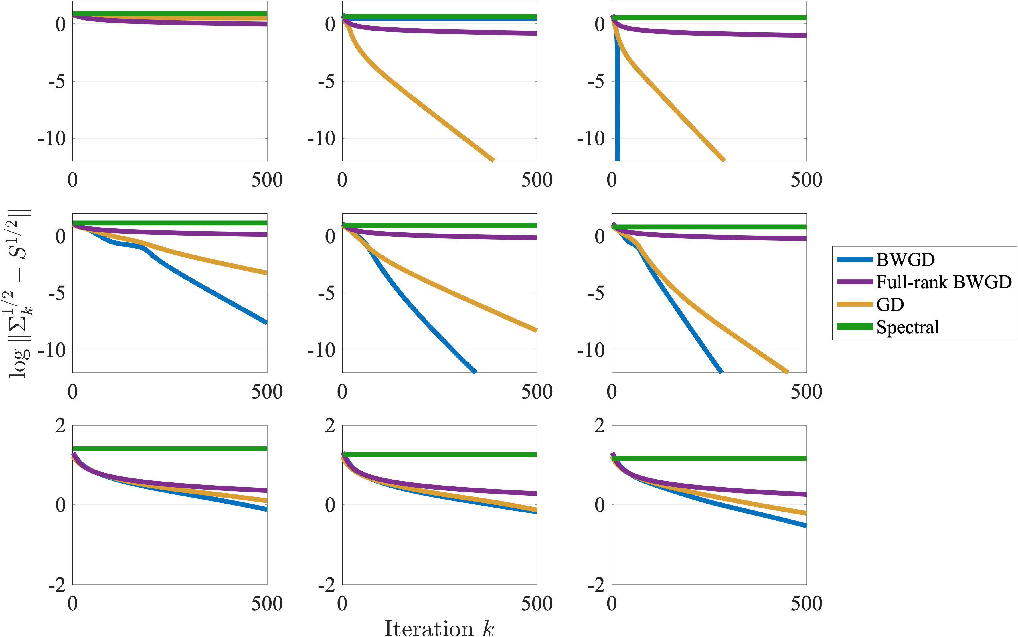
Figure 2: Convergence of BW gradient descent (2.14) with the full gradient and GD (Li et al., 2019).Here, $d=32$, and down the columns we use $r=1,4,16$, respectively. Across the rows we vary the number of points, with $n=3dr$, $n=10dr$, and $n=20dr$, respectively. As we can see, for low to moderate ranks, the BW gradient descent method converges much faster than the standard GD method.

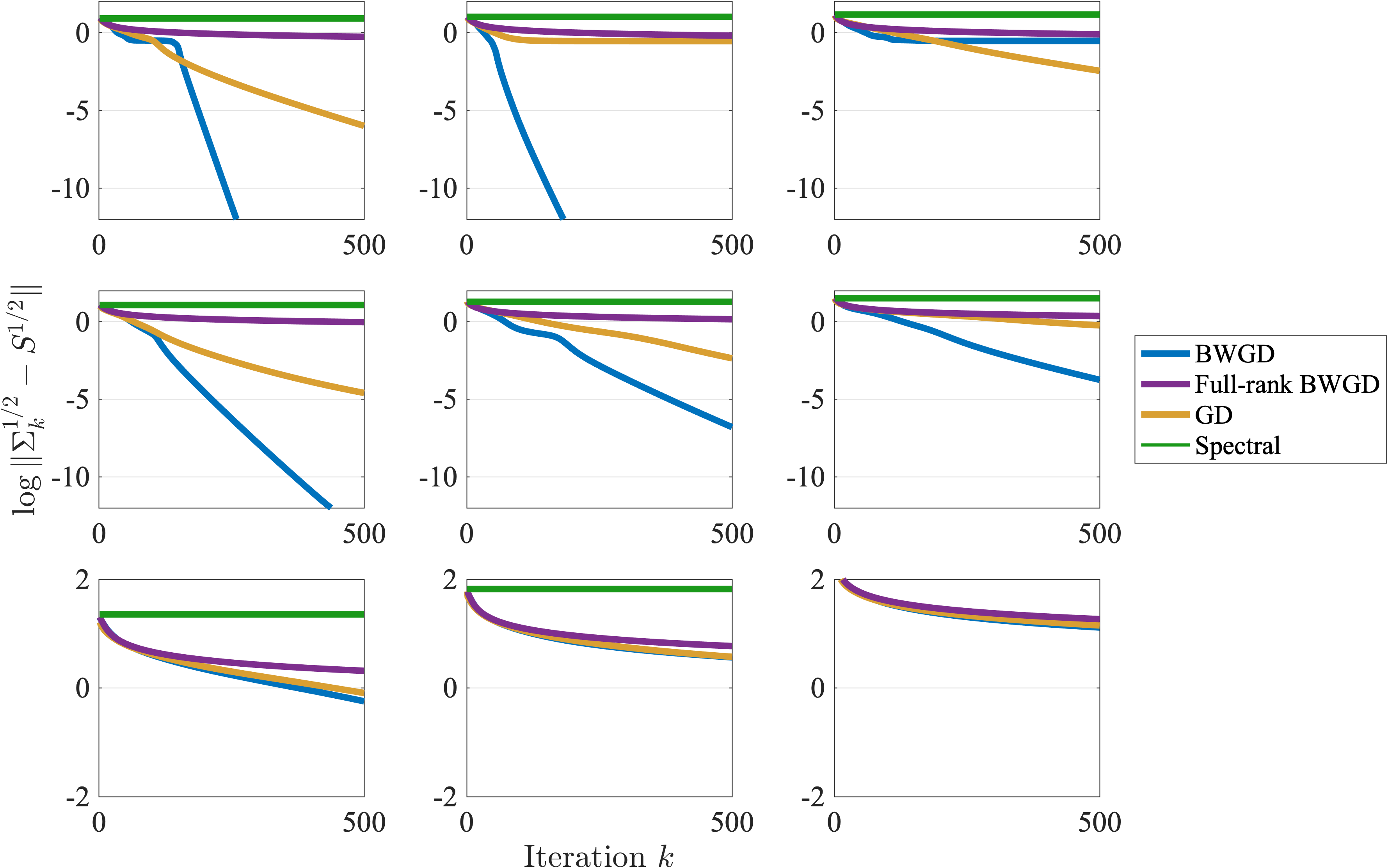
Figure 3: Convergence of BW gradient descent (2.14) with the full gradient and GD (Li et al., 2019). Here, $d=32$, and down the columns we use $r=2,4,16$, respectively. Across the rows we vary scale factor $\alpha$, with $\alpha=0,1,2$, respectively. As we can see, the BW gradient descent method converges much faster than the standard GD method.

4 Experiments

Here we present some numerical simulations that demonstrate the effectiveness of our method. All experiments were run on a 2020 Macbook Pro with a quad core CPU and 16 GB of RAM.

4.1 Synthetic Experiments

We begin with some experiments on generated datasets to better understand the performance of our method. Since our main results focus on the performance of gradient descent rather than stochastic gradient descent, we focus on its performance here.

The methods we compare are rank $r$ BW gradient descent, full rank BW gradient descent, the nonconvex Euclidean Gradient Descent (GD) of Li et al. (2019), and a spectral method, which takes a low-rank approximation to $\boldsymbol{S}_{n}=\frac{1}{2n}\sum_{i=1}^{n}y_{i}(\boldsymbol{x}_{i}\boldsymbol{x}_{i}^{\top}-\boldsymbol{I})$ since $\frac{1}{2}\mathbb{E}y^{2}(\boldsymbol{x}\boldsymbol{x}^{\top}-\boldsymbol{I})=\boldsymbol{S}$ (Sedghi et al., 2016). As an error metric, we compute $\|\boldsymbol{\Sigma}_{k}^{1/2}-\boldsymbol{S}^{1/2}\|_{F}=\Theta(d_{\mathrm{BW}}(\boldsymbol{\Sigma}_{k},\boldsymbol{S}))$. We do not compare with other matrix recovery algorithms since they are not guaranteed to work in the symmetric rank one projection setting. Also, we find the comparison with GD to be the most relevant, since BW gradient descent and GD have comparable complexity and are both first-order methods.

In our first experiment, we test the accuracy of the methods over time as we vary the rank of $\boldsymbol{S}$ and the sample size. Since the spectral method is not iterative, we include it as a horizontal line. Figure 2 displays the results of this experiment. Across the rows we vary the number of points and down the columns we vary the rank of $\boldsymbol{S}$. The fixed dimension is $d=32$, the ranks from top to bottom are $r=1,4,16$, and across the rows the number number points are $3dr$, $10dr$, and $20dr$, respectively. For each frame, we generate 20 datasets and run the four methods on them. All methods are run with random initialization, where the entries of $\boldsymbol{U}_{0}$ are i.i.d. $N(0,1)$. For $r=1$, we see that rank $r$ BW gradient descent succeeds once the number of points is sufficiently large. Furthermore, the convergence when it is successful is extremely fast. For moderate ranks, rank $r$ BW gradient descent converges faster than the previous GD method of Li et al. (2019).

In Figure 3, we examine the performance of the methods under varying conditioning of $\boldsymbol{S}$. We set $d=32$ and $n=5dr$ and vary $r$ as well as the conditioning of the matrix $S$. Here, $\boldsymbol{S}=\boldsymbol{V}\mathrm{diag}(r^{\alpha},(r-1)^{\alpha},\dots,1^{\alpha})\boldsymbol{V}^{\top}$, where the entries of $\boldsymbol{V}$ are i.i.d. $N(0,1)$ and $\alpha$ is a scale factor. Figure 3 displays the results on 20 randomly generated datasets per frame. The rows correspond to $r=2,4$, and $16$ respectively. The columns correspond to $\alpha=0,1$ and $2$ respectively. Rank $r$ BW gradient descent performs uniformly well throughout.

In Figure 4 we show the dependence on sample size. Here, $d=64$ and $r$ is varied from $1$ to $20$. The error of BW gradient descent and GD after 200 iterations is shown for sample sizes of $d$, $2d$, $\dots$, $20d$ for each value of $r$. For each $r,n$ pair, we generate 20 datasets and compute the average error across them. The color indicates the average error value across these datasets. As we see, BW gradient descent performs the best out of these methods. GD with linesearch is also competitive, but is more time consuming.

For the final synthetic experiment in Figure 5, we demonstrate the scalability of BW gradient descent to higher dimensions. We note that it scales much better in terms of actual computational time when compared with the Euclidean GD method of Li et al. (2019).

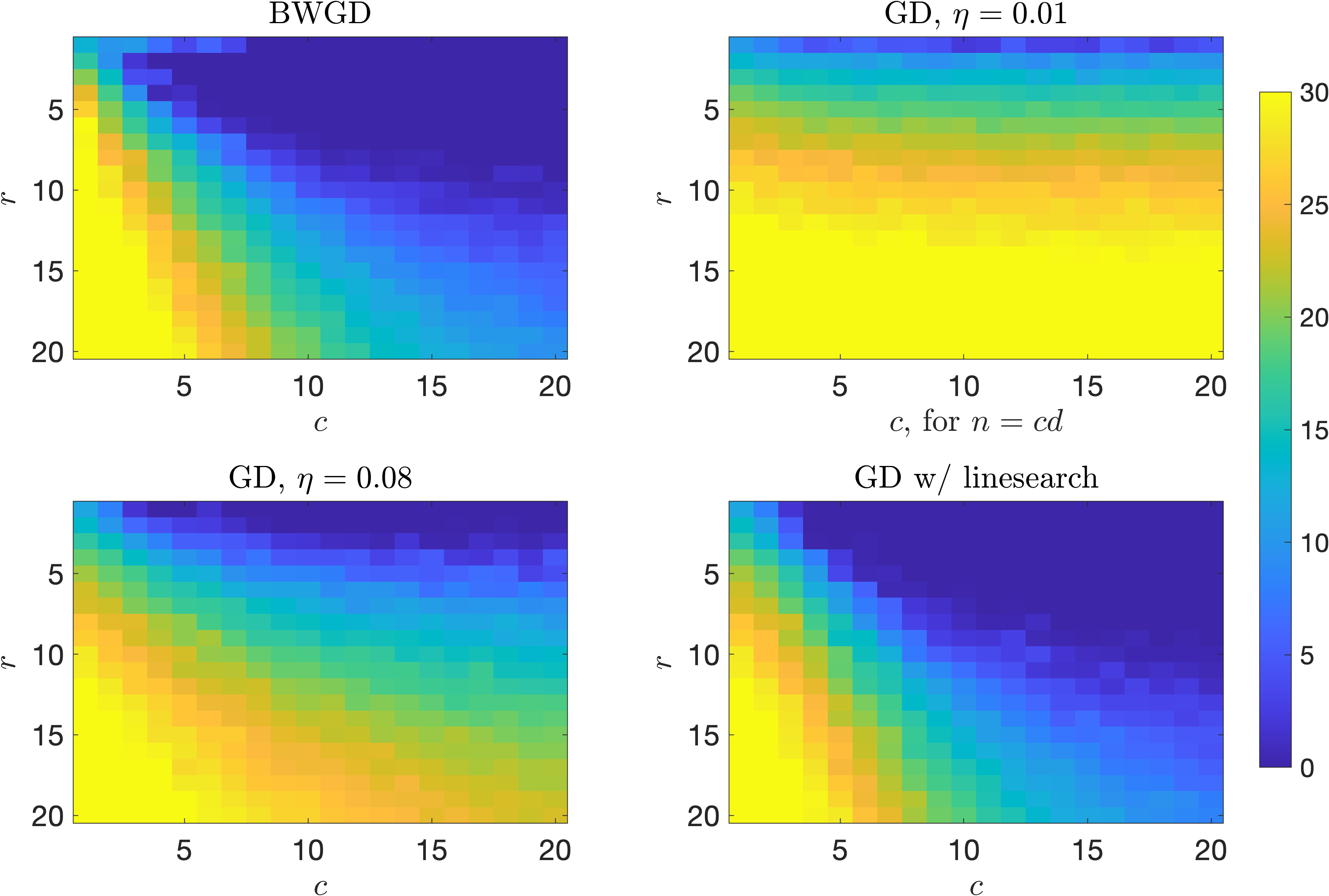
Figure 4: Convergence of BW gradient descent (2.14) with the full gradient and GD (Li et al., 2019). Here, $d=64$, and down the columns of each inset we use $r=1,\dots,20$, respectively. Across the rows we vary the scale factor $c$, where $n=cd$. As we can see, the BW gradient descent method converges much faster than the standard GD method with fixed step size, and performs on par with EGD with linesearch.

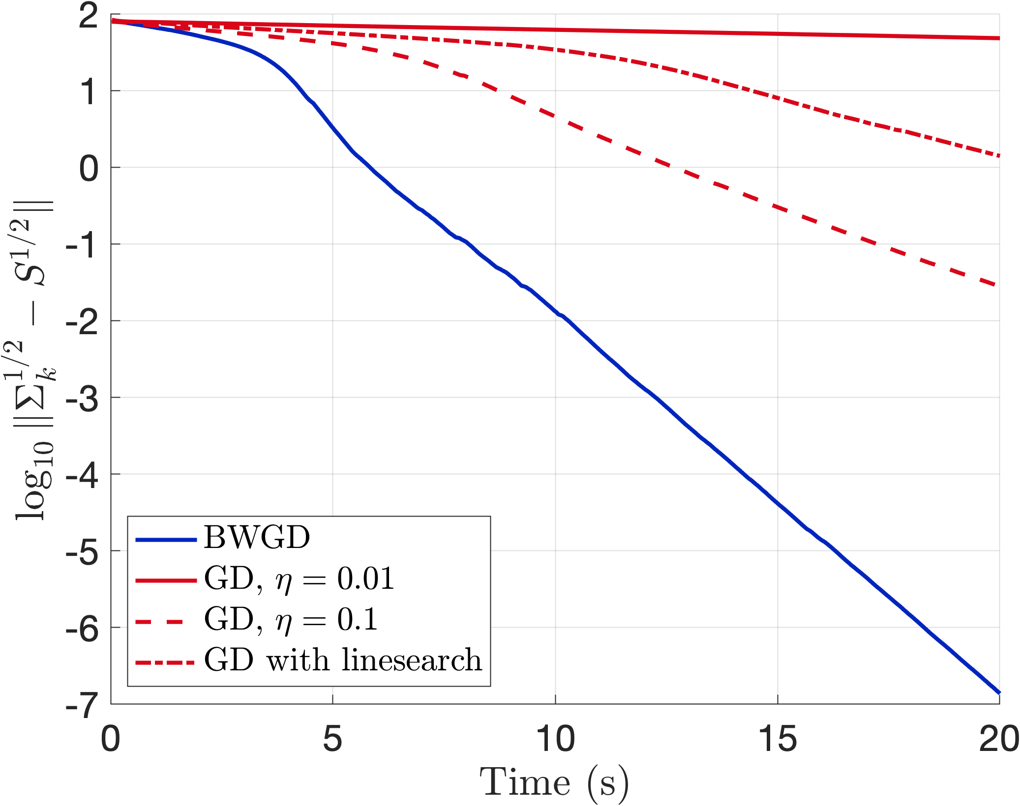
Figure 5: Convergence of BW gradient descent (2.14) and GD (Li et al., 2019). Here, $d=512$, $r=8$, and $n=3rd$. As we can see, the BW gradient descent method converges much faster than the standard GD method with any choice of step sizes. The per-iteration convergence rate for BW gradient descent is comparable to GD with linesearch, but doing linesearch increases computational burden.

4.2 Real Data Experiment: Phase Retrieval

Here we give the details of the experiment displayed in Figure 1. We replicate the phase retrieval experiments in Candès et al. (2015). In this paper, the authors study the nonconvex Wirtinger Flow algorithm. Since phase retrieval is equivalent to the recovery problem in (1.1) with a rank one complex $\boldsymbol{S}$, we can apply our algorithm in this setting.

Here, we use $i=\sqrt{-1}$. We use an image of Denali National Park, which is denoted by the 2-dimensional array $\boldsymbol{J}$ for each color band. In our simulated acquisition model, for $m=(u,v,\ell)$, we acquire data of the form

$$y_{m} =\Big{|}\sum_{j=1,k=1}^{j=d_{1},k=d_{2}}\boldsymbol{J}_{jk}\bar{d}_{\ell}(j,k)e^{-i2\pi(ju+kv)}\Big{|}^{2}.$$ (4.1)

Here, $d_{\ell}(j,k)\sim b_{1}b_{2}$, where $b_{1}$ is uniform on $\{1,-1,i,-i\}$, and $b_{2}$ takes values $\sqrt{2}/2$ with probability $4/5$ and $\sqrt{3}$ with probability $1/5$. The goal is to recover the image $\boldsymbol{J}$ from these measurements. We note that these measurements can be equivalently written as $y_{m}=\boldsymbol{F}_{u,v,\ell}^{\flat\top}\boldsymbol{J}^{\flat}\boldsymbol{J}^{\flat\top}\boldsymbol{F}_{u,v,\ell}^{\flat},$ where $\cdot^{\flat}$ denotes the vectorization operation and $\boldsymbol{F}$ is a matrix with entries $\bar{d}_{\ell}(j,k)e^{-i2\pi(ju+kv)}$. This notation makes clear the connection with the original matrix recovery problem in (1.1). We display the errors versus runtimes in Figure 6. Despite the fact that this example has $r=1$, BW gradient descent still efficiently recovers the underlying image, even though our current theory only works for $r\geq 3$.

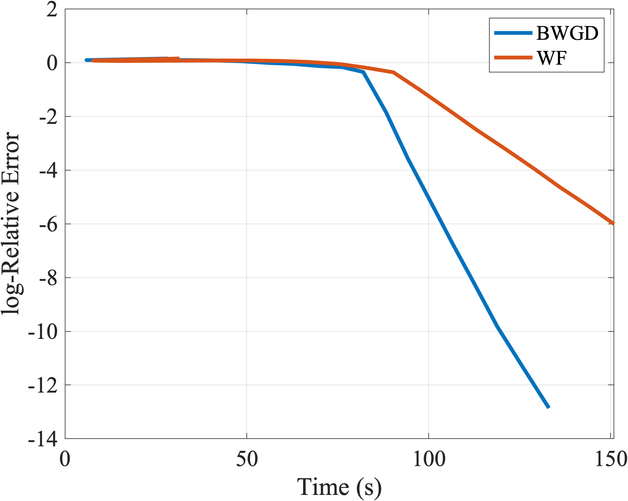
Figure 6: Error vs Runtime of BW gradient descent (our method) and Wirtinger Flow Candès et al. (2015) on the phase retrieval experiment in Figure 1. As we can see, BW gradient descent recovers the underlying image faster. Both methods are initialized with the power method as is done in (Candès et al., 2015).

5 Limitations

There are a few notable limitations for the current work. First of all, the theory does not directly extend to the cases of $r=1$ and $r=2$, and we must resort instead to the regularized methods discussed in Section 2.4. It is unclear whether or not this is a limitation of the methods or the analysis, although experiments indicate that the method works well for small dimensions in practice. Second, while our experiments indicate well-behaved energy landscapes, we are only able to prove local convergence results. Third, while we give the first optimization rates in terms of BW distance for this problem, our constants are not optimized. Fourth, we assume that one knows the rank of $S$ in advance. This is not a large issue since our framework allows for one to pick any $r^{\prime}\geq r$ and still recover $r$, albeit at a slower rate.

6 Conclusion

We have presented a novel connection between the BW barycenter problem and low-rank matrix recovery from rank one measurements. We show that a novel energy minimization problem coincides with the barycenter minimization. This connection allows us to extend algorithms from the barycenter problem to the matrix recovery problem, giving new algorithms for recovering low-rank PSD matrices. Our methods are guaranteed to have local linear convergence in BW distance, which is a stronger guarantee than existing methods.

This work leaves open many unexplored directions. For example, it would be interesting to show that the energy landscape does not exhibit spurious local minima. Beyond this, it would also be interesting to know when and how one can go beyond the RIP assumption, which currently relies on sub-Gaussianity of the sensing vectors. Finally, it would be interesting to connect these ideas to optimization landscapes for neural networks (Zhong et al., 2017; Du et al., 2019; Li et al., 2019).

7 Acknowledgements

PR is supported by NSF grants IIS-1838071, DMS-2022448, and CCF-2106377.

Appendix A Geometries of $\mathbb{S}_{+}^{d}$

Since the BW barycenter problem is inherently a geometric minimization problem over $\mathbb{S}_{+}^{d}$, we will quickly comment on how the choice of geometry effects optimization algorithms over this space.

There are many ways to define geometries over $\mathbb{S}_{+}^{d}$. For sake of comparison with previous methods for matrix recovery, we will compare BW space to the Euclidean geometry over PSD matrices. Among other things, the choice of geometry gives us a way of defining defining distance minimizing paths, or geodesics, over $\mathbb{S}_{+}^{d}$.

Consider two matrices $\boldsymbol{\Sigma}_{0},\boldsymbol{\Sigma}_{1}\in\mathbb{S}_{+}^{d}$ such that $\operatorname{rank}(\boldsymbol{\Sigma}_{0}\boldsymbol{\Sigma}_{1})=\operatorname{rank}(\boldsymbol{\Sigma}_{0})=\operatorname{rank}(\boldsymbol{\Sigma}_{1})$. This is a sufficient but not necessary condition to ensure that our following definition of BW geodesic is well defined since the same map can work for transporting higher rank PSD matrices to lower rank matrices. In any case, under this assumption, there exists a transport map from $\boldsymbol{\Sigma}_{0}$ to $\boldsymbol{\Sigma}_{1}$ given by

$$\boldsymbol{T}=\boldsymbol{\Sigma}_{1}^{1/2}(\boldsymbol{\Sigma}_{1}^{1/2}\boldsymbol{\Sigma}_{0}\boldsymbol{\Sigma}_{1}^{1/2})^{-1/2}\boldsymbol{\Sigma}_{1}^{1/2},$$ (A.1)

where the inverse is actually a pseudoinverse and one can check that $T\boldsymbol{\Sigma}_{0}T=\boldsymbol{\Sigma}_{1}$. In this case, the Euclidean and BW geodesics $\boldsymbol{\Sigma}_{t}:[0,1]\to\mathbb{S}_{+}^{d}$ are given by

$$\boldsymbol{\Sigma}_{t} =(1-t)\boldsymbol{\Sigma}_{0}+t\boldsymbol{\Sigma}_{1},$$ (EG)

$$\boldsymbol{\Sigma}_{t} =(\boldsymbol{I}+t(\boldsymbol{T}-\boldsymbol{I}))\boldsymbol{\Sigma}_{0}(I+t(\boldsymbol{T}-\boldsymbol{I})).$$ (BWG)

The first choice of geodesic, the Euclidean Geodesic (EG), corresponds to the distance functional $\|\boldsymbol{\Sigma}_{0}-\boldsymbol{\Sigma}_{1}\|_{F}$. The second choice of geodesic, the BW Geodesic (BWG), corresponds to the BW distance functional $d_{\mathrm{BW}}(\boldsymbol{\Sigma}_{0},\boldsymbol{\Sigma}_{1})$.

We note that (BWG) is equivalent to

$$\boldsymbol{\Sigma}_{t} =(I+t(\boldsymbol{T}-\boldsymbol{I}))\boldsymbol{\Sigma}_{0}(I+t(\boldsymbol{T}-\boldsymbol{I}))$$ (A.2)

$$=(\boldsymbol{\Sigma}_{0}^{1/2}+t\boldsymbol{\Delta})(\boldsymbol{\Sigma}_{0}^{1/2}+t\boldsymbol{\Delta})^{\top}.$$ (A.3)

where $\boldsymbol{\Delta}=(\boldsymbol{T}-\boldsymbol{I})\boldsymbol{\Sigma}_{0}^{1/2}$.

One of the big differences in these two paths is that while the Euclidean geodesics are linear in $t$, which is a result of the underlying flatness of the space, the BW geodesic contains terms that are quadratic in $t$. This points to the fact that this choice of geometry adds curvature to the space $\mathbb{S}_{+}^{d}$.

If we restrict ourselves to rank $r$ PSD matrices, $\mathbb{S}_{+}^{d,r}$, the geodesic (BWG) becomes

$$\boldsymbol{\Sigma}_{t} =(I+t(T-I)\boldsymbol{U}_{0}\boldsymbol{U}_{0}^{\top}(I+t(T-I))^{\top}$$ (A.4)

$$=((1-t)\boldsymbol{U}_{0}+t\boldsymbol{U}_{1})((1-t)\boldsymbol{U}_{0}+t\boldsymbol{U}_{1})^{\top},$$

where we use the fact that $\boldsymbol{T}\boldsymbol{\Sigma}_{0}\boldsymbol{T}=\boldsymbol{T}\boldsymbol{U}_{0}\boldsymbol{U}_{0}^{\top}\boldsymbol{T}=\boldsymbol{\Sigma}_{1}=\boldsymbol{U}_{1}\boldsymbol{U}_{1}^{\top}$. Note that there is an inherent rotational symmetry in the problem, since for any $R\in\mathbb{R}^{r\times r}$ such that $\boldsymbol{R}\boldsymbol{R}^{\top}=\boldsymbol{I}$ and $\boldsymbol{U}\boldsymbol{U}^{\top}\in\mathbb{S}_{+}^{d,r}$, $\boldsymbol{U}\boldsymbol{U}^{\top}=\boldsymbol{U}\boldsymbol{R}\boldsymbol{R}^{\top}U^{\top}$.

Appendix B Supplementary Proofs

B.1 Proof of Propositions 1 and 2

Proof of Proposition 1.

First, if $\frac{1}{n}\sum_{i}\boldsymbol{x}_{i}\boldsymbol{x}_{i}^{\top}=\boldsymbol{I}$, then

$$\frac{1}{n}\sum_{i}\mathcal{A}(\boldsymbol{\Sigma})_{i}=\operatorname{Tr}(\boldsymbol{\Sigma}).$$

Indeed, this follows from the fact that

$$\frac{1}{n}\sum_{i}\mathcal{A}(\boldsymbol{\Sigma})_{i}=\frac{1}{n}\sum_{i}\boldsymbol{x}_{i}^{\top}\boldsymbol{\Sigma}\boldsymbol{x}_{i}=\operatorname{Tr}\left(\boldsymbol{\Sigma}\frac{1}{n}\sum_{i}\boldsymbol{x}_{i}\boldsymbol{x}_{i}^{\top}\right)=\operatorname{Tr}(\boldsymbol{\Sigma}).$$ (B.1)

With this in mind, we expand the square in (2.4)

$$\frac{1}{2n}\|\sqrt{\mathcal{A}(\boldsymbol{\Sigma})}-\sqrt{y}\|_{2}^{2}=$$ (B.2)

$$\frac{1}{2n}\sum_{i}\mathcal{A}(\boldsymbol{\Sigma})_{i}+\frac{1}{2n}\sum_{i}y_{\boldsymbol{I}}-\frac{1}{n}\sum_{i}\sqrt{y_{i}}\sqrt{\boldsymbol{x}_{i}^{\top}\boldsymbol{\Sigma}\boldsymbol{x}_{i}}$$

$$=\frac{1}{2}\operatorname{Tr}(\boldsymbol{\Sigma})-\frac{1}{n}\sum_{i}\sqrt{y_{i}}\sqrt{\boldsymbol{x}_{i}^{\top}\boldsymbol{\Sigma}\boldsymbol{x}_{i}}+\frac{1}{2n}\sum_{i}y_{i}.$$

Thus, the minimization in (2.4) is equivalent to the program

$$\min_{\boldsymbol{\Sigma}\in\mathbb{S}_{+}^{d}}\operatorname{Tr}(\boldsymbol{\Sigma})-\frac{2}{n}\sum_{i=1}^{n}\sqrt{y_{i}}\sqrt{\boldsymbol{x}_{i}^{\top}\boldsymbol{\Sigma}\boldsymbol{x}_{i}}$$ (B.3)

On the other hand, it is not hard to show that the BW distance between a matrix $\boldsymbol{\Sigma}\in\mathbb{S}_{+}^{d}$ and a rank one matrix $\boldsymbol{w}\boldsymbol{w}^{\top}$ is

$$d_{\mathrm{BW}}^{2}(\boldsymbol{\Sigma},\boldsymbol{w}\boldsymbol{w}^{\top})=\Big{[}\operatorname{Tr}(\boldsymbol{\Sigma})+\operatorname{Tr}(\boldsymbol{x}\boldsymbol{x}^{\top})-2\sqrt{\operatorname{Tr}(\boldsymbol{x}\boldsymbol{x}^{\top}\boldsymbol{\Sigma})}\Big{]}.$$ (B.4)

Letting $\boldsymbol{w}\boldsymbol{w}^{\top}=y_{i}\boldsymbol{x}_{i}\boldsymbol{x}_{i}^{\top}$ and summing over $i$, we see that (B.3) is equivalent to minimizing (2.8) when

$$Q=\frac{1}{n}\sum_{i=1}^{n}\delta_{y_{i}\boldsymbol{x}_{i}\boldsymbol{x}_{i}^{\top}}.$$

∎

Proof of Proposition 2.

Consider the first order condition for the $n$ rank one matrices $y_{i}^{2}\boldsymbol{C}_{n}^{-1/2}\boldsymbol{x}_{i}\boldsymbol{x}_{i}^{\top}\boldsymbol{C}_{n}^{-1/2}$ given by

$$\frac{1}{n}\sum_{i=1}^{n}\frac{\operatorname{Tr}(\boldsymbol{x}_{i}\boldsymbol{x}_{i}^{\top}\boldsymbol{S})^{1/2}}{\operatorname{Tr}(\boldsymbol{C}_{n}^{-1/2}\boldsymbol{x}_{i}\boldsymbol{x}_{i}^{\top}\boldsymbol{C}_{n}^{-1/2}\boldsymbol{\Sigma}_{n})^{1/2}}\boldsymbol{C}_{n}^{-1/2}\boldsymbol{x}_{i}\boldsymbol{x}_{i}^{\top}\boldsymbol{C}_{n}^{-1/2}=\boldsymbol{I}.$$ (B.5)

Since $\boldsymbol{C}_{n}^{-1/2}\boldsymbol{C}_{n}\boldsymbol{C}_{n}^{-1/2}=\boldsymbol{I}$, we see that $\boldsymbol{C}_{n}^{-1/2}\boldsymbol{\Sigma}_{n}\boldsymbol{C}_{n}^{-1/2}=\boldsymbol{S}$ is a sufficient condition for $\boldsymbol{\Sigma}_{n}$ to be a barycenter of

$$Q=\frac{1}{n}\sum_{i=1}^{n}\delta_{y_{i}\boldsymbol{C}_{n}^{-1/2}\boldsymbol{x}_{i}\boldsymbol{x}_{i}^{\top}\boldsymbol{C}_{n}^{-1/2}}$$ (B.6)

∎

B.2 Proof of Theorem 3

The proof of Theorem 3 proceeds in the following sections. In Section B.2.1, we establish some restricted isometry properties (RIP) that will be used in our proof. Then, Section B.2.2 proves that the function $F$ is Euclidean strongly convex over $\mathbb{S}_{+}^{d}$ with high probability. After this, Section B.2.3 shows that $F$ also satisfies a certain Euclidean smoothness over rank $r$ matrices. Section B.2.4 discusses first order optimality conditions for the barycenter, and in particular gives sufficient conditions for a point $\overline{\boldsymbol{\Sigma}}$ to be the minimizer of $F$. Section B.2.5 gives a descent lemma for the fixed-rank gradient descent method. After this, Section B.2.6 proves local strong convexity of $F$ over fixed-rank PSD matrices in $\mathbb{S}_{+}^{d,r}$ that are close to $S$. We finish in Section B.2.7 by putting all of these facts together.

B.2.1 RIP Conditions

We discuss here a case an RIP condition that becomes essential for our later proof. As discussed in Cai and Zhang [2015], issues arise in trying to prove a full $\ell_{2}$ RIP for this problem, due to the fact that the fourth moments of $\boldsymbol{x}$ that show up. Instead, both Cai and Zhang [2015], Chen et al. [2015] prove the following $\ell_{2}/\ell_{1}$ RIP condition (also referred to as “Restricted Uniform Boundedness").

Theorem 8 (Chen et al. [2015] Proposition 1).

Suppose that $\boldsymbol{x}_{1},\dots,\boldsymbol{x}_{n}$ are a sample from a sub-Gaussian distribution with $\mathbb{E}\boldsymbol{x}_{i}=\boldsymbol{0}$, $\mathbb{E}x_{ij}^{2}=1$, and $\mathbb{E}x_{ij}^{4}>1$. Then, there are constants $c_{1},c_{2},c_{3}>0$ such that with probability exceeding $1-\exp(-c_{3}n)$

$$c_{1}\|\boldsymbol{\Delta}\|_{F}\leq\frac{1}{n}\left\|\begin{bmatrix}\boldsymbol{x}_{1}^{\top}\boldsymbol{\Delta}\boldsymbol{x}_{1}-\boldsymbol{x}_{2}^{\top}\boldsymbol{\Delta}\boldsymbol{x}_{2}\\ \boldsymbol{x}_{3}^{\top}\boldsymbol{\Delta}\boldsymbol{x}_{3}-\boldsymbol{x}_{4}^{\top}\boldsymbol{\Delta}\boldsymbol{x}_{4}\\ \vdots\\ \boldsymbol{x}_{n-1}^{\top}\boldsymbol{\Delta}\boldsymbol{x}_{n-1}-\boldsymbol{x}_{n}^{\top}\boldsymbol{\Delta}\boldsymbol{x}_{n}\end{bmatrix}\right\|_{1}\leq c_{2}\|\boldsymbol{\Delta}\|_{F}.$$ (B.7)

hold simultaneously for all rank $r$ matrices $\boldsymbol{\Delta}$ provided that $n\gtrsim dr$.

We have the following corollary to this theorem.

Corollary 9.

Suppose that a random vector $\boldsymbol{w}=(w_{1},\dots,w_{d})^{\top}$ is sub-Gaussian with $\mathbb{E}\boldsymbol{w}=\boldsymbol{0}$, $\mathbb{E}w_{j}^{2}=1$, $\mathbb{E}w_{j}^{4}>1$. Then, the following population RIP holds:

$$\mathbb{E}_{\boldsymbol{w}}\operatorname{Tr}(\boldsymbol{w}\boldsymbol{w}^{\top}\boldsymbol{A})^{2}\geq c_{1}\|\boldsymbol{A}\|_{F}^{2}.$$ (B.8)

Furthermore, for a sample of $n$ i.i.d. copies of $W$, $\boldsymbol{w}_{1},\dots,\boldsymbol{w}_{n}$, there are constants $c_{2},c_{3}>0$ such that with probability exceeding $1-\exp(-c_{3}n)$

$$\frac{1}{n}\sum_{i=1}^{n}\operatorname{Tr}(\boldsymbol{w}_{i}\boldsymbol{w}_{i}^{\top}\boldsymbol{A})^{2}\geq c_{2}\|\boldsymbol{A}\|_{F}^{2}$$ (B.9)

hold simultaneously for all rank $r$ matrices $\boldsymbol{\Delta}$ provided that $n\gtrsim dr$.

Proof.

The first part holds from the argument in Appendix A of Chen et al. [2015].

For the second part, we compute

$$\frac{1}{n}\sum_{i=1}^{n}\operatorname{Tr}(\boldsymbol{w}_{i}\boldsymbol{w}_{i}^{\top}\boldsymbol{A})^{2} =\frac{1}{n}\sum_{i=1}^{n}\operatorname{Tr}(\boldsymbol{w}_{i}\boldsymbol{w}_{i}^{\top}\boldsymbol{A})^{2}$$ (B.10)

$$=\frac{1}{n}\sum_{i=1}^{n/2}\operatorname{Tr}(\boldsymbol{w}_{2i}\boldsymbol{w}_{2i}^{\top}\boldsymbol{A})^{2}+\operatorname{Tr}(\boldsymbol{w}_{2i-1}\boldsymbol{w}_{2i-1}^{\top}\boldsymbol{A})^{2}$$

$$\geq\frac{1}{2n}\sum_{i=1}^{n/2}[\operatorname{Tr}(\boldsymbol{w}_{2i}\boldsymbol{w}_{2i}^{\top}\boldsymbol{A})-\operatorname{Tr}(\boldsymbol{w}_{2i-1}\boldsymbol{w}_{2i-1}^{\top}\boldsymbol{A})]^{2}$$

$$=\frac{1}{n^{2}}\frac{n}{2}\sum_{i=1}^{n/2}[\operatorname{Tr}(\boldsymbol{w}_{2i}\boldsymbol{w}_{2i}^{\top}\boldsymbol{A})-\operatorname{Tr}(\boldsymbol{w}_{2i-1}\boldsymbol{w}_{2i-1}^{\top}\boldsymbol{A})]^{2}$$

$$\geq\frac{1}{n^{2}}\Big{[}\sum_{i=1}^{n/2}|\operatorname{Tr}(\boldsymbol{w}_{2i}\boldsymbol{w}_{2i}^{\top}\boldsymbol{A})-\operatorname{Tr}(\boldsymbol{w}_{2i-1}\boldsymbol{w}_{2i-1}^{\top}\boldsymbol{A})|\Big{]}^{2}$$

$$\geq c_{2}^{2}\|\boldsymbol{A}\|_{F}^{2}.$$

∎

B.2.2 Euclidean Strong Convexity

We begin by proving strong convexity along Euclidean geodesics. In particular, this guarantees that $S$ is the unique minimizer of $F$ over $\mathbb{S}_{+}^{d}$. Furthermore, it shows that $S$ is the unique stationary point.

First, it is easy to see that $S$ is stationary because

$$\nabla F(\boldsymbol{S})=\boldsymbol{I}-\mathbb{E}_{Q}\sqrt{\frac{\boldsymbol{x}^{\top}\boldsymbol{S}\boldsymbol{x}}{\boldsymbol{x}^{\top}\boldsymbol{S}\boldsymbol{x}}}\boldsymbol{x}\boldsymbol{x}^{\top}=\boldsymbol{I}-\mathbb{E}_{Q}\boldsymbol{x}\boldsymbol{x}^{\top}=0.$$ (B.11)

Define the set

$$\mathcal{S}(m,M)=\{\boldsymbol{\Sigma}\in\mathbb{S}_{+}^{d}:m\leq\lambda_{r}(\boldsymbol{\Sigma})\leq\lambda_{1}(\boldsymbol{\Sigma})\leq M\}.$$ (B.12)

We have the following lemma over this set.

Lemma 10.

Let $y=\langle\boldsymbol{x}\boldsymbol{x}^{\top},\boldsymbol{S}\rangle$, where $\boldsymbol{x}\sim N(\boldsymbol{0},\boldsymbol{I})$, $\boldsymbol{S}$ is rank $r$, and $m,M$ be such that $\boldsymbol{S}\in\mathcal{S}(m,M)$. Then, the population obective $F$ is Euclidean strongly convex over $\mathcal{S}(0,M)$ with constant $\frac{c_{1}\beta^{2}d}{6M^{3/2}}$.

In other words, the function $F(\boldsymbol{\Sigma}_{t})$ is strongly convex when $\boldsymbol{\Sigma}_{t}$ is defined by (EG).

Proof.

Let $\boldsymbol{\Sigma}_{t}$ denote the geodesic between $\boldsymbol{\Sigma}_{0}$ and $\boldsymbol{\Sigma}_{1}$ given by $(1-t)\boldsymbol{\Sigma}_{0}+t\boldsymbol{\Sigma}_{1}$. We compute the derivatives of the BW distance as

$$\partial_{t}d_{\mathrm{BW}}(\boldsymbol{\Sigma}_{t},\boldsymbol{x}\boldsymbol{x}^{\top})^{2} =\operatorname{Tr}(\boldsymbol{\Sigma}_{1}-\boldsymbol{\Sigma}_{0})$$ (B.13)

$$-\frac{\operatorname{Tr}((\boldsymbol{\Sigma}_{1}-\boldsymbol{\Sigma}_{0})\boldsymbol{x}\boldsymbol{x}^{\top})}{\sqrt{\boldsymbol{x}^{\top}\boldsymbol{\Sigma}_{t}\boldsymbol{x}}},$$ (B.14)

$$\partial_{t}^{2}d_{\mathrm{BW}}(\boldsymbol{\Sigma}_{t},\boldsymbol{x}\boldsymbol{x}^{\top})^{2} =\frac{1}{2}\frac{\operatorname{Tr}(\boldsymbol{x}\boldsymbol{x}^{\top}(\boldsymbol{\Sigma}_{1}-\boldsymbol{\Sigma}_{0}))^{2}}{\operatorname{Tr}(\boldsymbol{x}\boldsymbol{x}^{\top}\boldsymbol{\Sigma}_{t})^{3/2}}$$ (B.15)

By the definition of $M$, we have the uniform bound

$$\partial_{t}^{2}F(\boldsymbol{\Sigma}_{t})|_{t=s}=\mathbb{E}_{\boldsymbol{x}\boldsymbol{x}^{\top}\sim Q}\frac{1}{2}\frac{\operatorname{Tr}(\boldsymbol{x}\boldsymbol{x}^{\top}(\boldsymbol{\Sigma}_{1}-\boldsymbol{\Sigma}_{0}))^{2}}{(\operatorname{Tr}(\boldsymbol{x}\boldsymbol{x}^{\top}\boldsymbol{\Sigma}_{s}))^{3/2}}$$ (B.16)

$$=\mathbb{E}_{\boldsymbol{x}\boldsymbol{x}^{\top}\sim Q}\frac{1}{2\|\boldsymbol{x}\|^{3}}\frac{\operatorname{Tr}(\boldsymbol{x}\boldsymbol{x}^{\top}(\boldsymbol{\Sigma}_{1}-\boldsymbol{\Sigma}_{0}))^{2}}{(\operatorname{Tr}(\boldsymbol{x}\boldsymbol{x}^{\top}\boldsymbol{\Sigma}_{s}/\|\boldsymbol{x}\|^{2}))^{3/2}}$$

$$\geq\frac{1}{2(2M)^{3/2}}\mathbb{E}_{\boldsymbol{x}\boldsymbol{x}^{\top}\sim Q}\frac{1}{\|\boldsymbol{x}\|^{3}}\operatorname{Tr}(\boldsymbol{x}\boldsymbol{x}^{\top}(\boldsymbol{\Sigma}_{1}-\boldsymbol{\Sigma}_{0}))^{2}.$$

Using the definition $\boldsymbol{w}\boldsymbol{w}^{\top}=(\boldsymbol{x}^{\top}\boldsymbol{S}\boldsymbol{x})\boldsymbol{x}\boldsymbol{x}^{\top}$,

$$\partial_{t}^{2}F(\boldsymbol{\Sigma}_{t})|_{t=s} \geq\frac{1}{6M^{3/2}}\mathbb{E}_{\boldsymbol{x}\sim N(\boldsymbol{0},\boldsymbol{I})}\frac{\sqrt{\boldsymbol{x}^{\top}\boldsymbol{S}\boldsymbol{x}}}{\|\boldsymbol{x}\|^{3}}\operatorname{Tr}(\boldsymbol{x}\boldsymbol{x}^{\top}(\boldsymbol{\Sigma}_{1}-\boldsymbol{\Sigma}_{0}))^{2}$$ (B.17)

$$\geq\frac{1}{6M^{3/2}}\mathbb{E}_{\boldsymbol{x}\sim N(\boldsymbol{0},\boldsymbol{I})}|X\|^{2}\sqrt{\frac{\boldsymbol{x}^{\top}\boldsymbol{S}\boldsymbol{x}}{\|\boldsymbol{x}\|^{2}}}\operatorname{Tr}(\frac{\boldsymbol{x}\boldsymbol{x}^{\top}}{\|\boldsymbol{x}\|^{2}}(\boldsymbol{\Sigma}_{1}-\boldsymbol{\Sigma}_{0}))^{2}$$

$$=\frac{d}{6M^{3/2}}\mathbb{E}_{\boldsymbol{x}\sim N(\boldsymbol{0},\boldsymbol{I})}\sqrt{\frac{\boldsymbol{x}^{\top}\boldsymbol{S}\boldsymbol{x}}{\|\boldsymbol{x}\|^{2}}}\operatorname{Tr}(\frac{\boldsymbol{x}\boldsymbol{x}^{\top}}{\|\boldsymbol{x}\|^{2}}(\boldsymbol{\Sigma}_{1}-\boldsymbol{\Sigma}_{0}))^{2}.$$

Define the random vector

$$W:=\Big{(}\frac{\boldsymbol{x}^{\top}\boldsymbol{S}\boldsymbol{x}}{\|\boldsymbol{x}\|^{2}}\Big{)}^{1/8}\frac{\boldsymbol{x}}{\|\boldsymbol{x}\|}.$$ (B.18)

By symmetry, $\boldsymbol{w}$ is mean zero. Furthermore, $\boldsymbol{w}$ is bounded and thus sub-Gaussian. Furthermore, it is a simple exercise to show that

$$\boldsymbol{C}_{W}:=\mathbb{E}\boldsymbol{w}\boldsymbol{w}^{\top}\succeq\beta\boldsymbol{I},$$ (B.19)

for some dimension and $\boldsymbol{S}$-dependent constant $\beta$. We can thus bound

$$\mathbb{E}_{\boldsymbol{x}}\operatorname{Tr}\left(\boldsymbol{w}\boldsymbol{w}^{\top}(\boldsymbol{\Sigma}_{1}-\boldsymbol{\Sigma}_{0})\right)^{2} =\mathbb{E}_{W}\operatorname{Tr}\left(\boldsymbol{C}_{W}^{1/2}\boldsymbol{C}_{W}^{-1/2}\boldsymbol{w}\boldsymbol{w}^{\top}\boldsymbol{C}_{W}^{-1/2}\boldsymbol{C}_{W}^{1/2}(\boldsymbol{\Sigma}_{1}-\boldsymbol{\Sigma}_{0})\right)^{2}$$ (B.20)

$$\geq\beta^{2}\mathbb{E}_{W}\operatorname{Tr}(\boldsymbol{C}_{W}^{-1/2}\boldsymbol{w}\boldsymbol{w}^{\top}\boldsymbol{C}_{W}^{-1/2}(\boldsymbol{\Sigma}_{1}-\boldsymbol{\Sigma}_{0}))^{2}.$$

Using the fact that $\boldsymbol{C}_{W}^{-1/2}\boldsymbol{w}$ is mean zero sub-Gaussian with identity covariance (and furthermore the 4th moment condition is trivially satisfied), we can now use the RIP condition of Corollary 9 to bound

$$\mathbb{E}_{\boldsymbol{w}\boldsymbol{w}^{\top}\sim Q}\operatorname{Tr}(\boldsymbol{C}_{W}^{-1/2}\boldsymbol{w}\boldsymbol{w}^{\top}\boldsymbol{C}_{W}^{-1/2}(\boldsymbol{\Sigma}_{1}-\boldsymbol{\Sigma}_{0}))^{2}\geq c_{1}\|\boldsymbol{\Sigma}_{1}-\boldsymbol{\Sigma}_{0}\|_{F}^{2}.$$ (B.21)

Putting this all together,

$$\partial_{t}^{2}F(\boldsymbol{\Sigma}_{t})|_{t=s} \geq\frac{c_{1}\beta^{2}d}{2(2M)^{3/2}}\|\boldsymbol{\Sigma}_{1}-\boldsymbol{\Sigma}_{0}\|_{F}^{2}$$ (B.22)

$$\geq\frac{c_{1}\beta^{2}d}{6M^{3/2}}\|\boldsymbol{\Sigma}_{1}-\boldsymbol{\Sigma}_{0}\|_{F}^{2}.$$

∎

The sample setting requires a bit more work. In this case, we observe ${y}_{i}$ and $\boldsymbol{x}_{i}$, $i=1,\dots,n$, and to recover the matrix $S$ we first compute the barycenter of ${y}_{i}\boldsymbol{C}_{n}^{-1/2}\boldsymbol{x}_{i}\boldsymbol{x}_{i}^{\top}\boldsymbol{C}_{n}^{-1/2}$, where $\boldsymbol{C}_{n}$ is the sample covariance. We denote this whitened discrete distribution by $\tilde{Q}$. In this case, by Proposition 2, the barycenter is $\overline{\boldsymbol{\Sigma}}=\boldsymbol{C}_{n}^{-1/2}S\boldsymbol{C}_{n}^{-1/2}$

Lemma 11.

With probability at least $1-\exp(-c_{2}n)$ for some constant $c_{2}$, $F$ is Euclidean strongly convex over $\mathcal{S}(0,M)$ with constant $\frac{c_{3}\beta^{2}d}{6M^{3/2}}$.

Proof.

In this case,

$$\partial_{t}^{2}F(\boldsymbol{\Sigma}_{t})|_{t=s} \geq\frac{1}{6M^{3/2}}\frac{1}{n}\sum_{i=1}^{n}\frac{\sqrt{\boldsymbol{x}_{i}^{\top}\boldsymbol{S}\boldsymbol{x}_{i}}}{\|\boldsymbol{C}_{n}^{-1/2}\boldsymbol{x}_{i}\|^{3}}\operatorname{Tr}(\boldsymbol{C}_{n}^{-1/2}\boldsymbol{x}_{i}\boldsymbol{x}_{i}^{\top}\boldsymbol{C}_{n}^{-1/2}(\overline{\boldsymbol{\Sigma}}-\boldsymbol{\Sigma}))^{2}$$ (B.23)

$$\geq\frac{1}{6M^{3/2}}\frac{\lambda_{\min}(\boldsymbol{C}_{n})^{3/2}}{\lambda_{\max}(\boldsymbol{C}_{n})^{2}}\frac{1}{n}\sum_{i=1}^{n}\frac{\sqrt{\boldsymbol{x}_{i}^{\top}\boldsymbol{S}\boldsymbol{x}_{i}}}{\|\boldsymbol{x}_{i}\|^{3}}\operatorname{Tr}(\boldsymbol{x}_{i}\boldsymbol{x}_{i}^{\top}(\overline{\boldsymbol{\Sigma}}-\boldsymbol{\Sigma}))^{2}$$

$$=\frac{1}{6M^{3/2}}\frac{\lambda_{\min}(\boldsymbol{C}_{n})^{3/2}}{\lambda_{\max}(\boldsymbol{C}_{n})^{2}}\frac{1}{n}\sum_{i=1}^{n}\operatorname{Tr}\Big{(}\|\boldsymbol{x}_{i}\|\Big{(}\frac{\boldsymbol{x}_{i}^{\top}\boldsymbol{S}\boldsymbol{x}_{i}}{\|\boldsymbol{x}_{i}\|^{2}}\Big{)}^{1/4}\frac{\boldsymbol{x}_{i}\boldsymbol{x}_{i}^{\top}}{\|\boldsymbol{x}_{i}\|^{2}}(\overline{\boldsymbol{\Sigma}}-\boldsymbol{\Sigma})\Big{)}^{2}.$$

Then, following the same line of reasoning as in the previous proof to obtain strong convexity the sub-Gaussianity of the random vector

$$\boldsymbol{w}_{i}=\|\boldsymbol{x}_{i}\|^{1/2}\Big{(}\frac{\boldsymbol{x}_{i}^{\top}\boldsymbol{S}\boldsymbol{x}_{i}}{\|\boldsymbol{x}_{i}\|^{2}}\Big{)}^{1/8}\frac{\boldsymbol{x}_{i}}{\|\boldsymbol{x}_{i}\|},$$ (B.24)

which again a simple exercise shows $\mathbb{E}\boldsymbol{w}_{i}\boldsymbol{w}_{i}^{\top}\succeq\beta\boldsymbol{I}$ and $\mathbb{E}\boldsymbol{w}_{i}=0$. Then, with probability at least $1-\exp(-c_{2}n)$, the discrete distribution is strongly convex with constant $\frac{c_{3}\beta^{2}d}{6M^{3/2}}$. ∎

Notice that in both the population and the sample setting with high probability we get a unique barycenter $S$.

B.2.3 Local Euclidean Smoothness

We remind ourselves that

$$\nabla F(\boldsymbol{\Sigma})=\boldsymbol{I}-\mathbb{E}_{Q}\sqrt{\frac{\boldsymbol{x}^{\top}\boldsymbol{S}\boldsymbol{x}}{\boldsymbol{x}^{\top}\boldsymbol{\Sigma}\boldsymbol{x}}}\boldsymbol{x}\boldsymbol{x}^{\top},$$ (B.25)

Using this, we have the following lemma.

Lemma 12.

Let $y=\langle\boldsymbol{x}\boldsymbol{x}^{\top},\boldsymbol{S}$, $X\sim N(\boldsymbol{0},\boldsymbol{I})$, $\operatorname{rank}(\boldsymbol{\Sigma})\geq 3$, and $\lambda_{r}(\boldsymbol{\Sigma})\geq m$. Then,

$$\left\|\nabla F(\boldsymbol{S})-\nabla F(\boldsymbol{\Sigma})\right\|_{F}=\left\|\nabla F(\boldsymbol{\Sigma})\right\|_{F}\leq\frac{d^{3/2}}{m\sqrt{r}}\|\boldsymbol{\Sigma}-\boldsymbol{S}\|_{F}$$ (B.26)

Proof.

We have that

$$\left\|\mathbb{E}_{Q}\sqrt{\frac{\boldsymbol{x}^{\top}\boldsymbol{S}\boldsymbol{x}}{\boldsymbol{x}^{\top}\boldsymbol{S}\boldsymbol{x}}}\boldsymbol{x}\boldsymbol{x}^{\top}-\mathbb{E}_{Q}\sqrt{\frac{\boldsymbol{x}^{\top}\boldsymbol{S}\boldsymbol{x}}{\boldsymbol{x}^{\top}\boldsymbol{\Sigma}\boldsymbol{x}}}\boldsymbol{x}\boldsymbol{x}^{\top}\right\| \leq\mathbb{E}_{Q}\left|\frac{\sqrt{\boldsymbol{x}^{\top}\boldsymbol{\Sigma}\boldsymbol{x}}-\sqrt{\boldsymbol{x}^{\top}\boldsymbol{S}\boldsymbol{x}}}{\sqrt{\boldsymbol{x}^{\top}\boldsymbol{\Sigma}\boldsymbol{x}}}\right|\|\boldsymbol{x}\|^{2}$$ (B.27)

$$=d\mathbb{E}_{Q}\frac{1}{\sqrt{\boldsymbol{x}^{\top}\boldsymbol{\Sigma}\boldsymbol{x}}}\sqrt{|\boldsymbol{x}^{\top}(\boldsymbol{\Sigma}-\boldsymbol{S})\boldsymbol{x}|}$$

$$\leq d\|\boldsymbol{\Sigma}-\boldsymbol{S}\|_{F}^{1/2}\mathbb{E}_{Q}\frac{\|\boldsymbol{x}\|}{\sqrt{\boldsymbol{x}^{\top}\boldsymbol{\Sigma}\boldsymbol{x}}}$$

As long as $r\geq 3$ and $\lambda_{r}(\boldsymbol{\Sigma})\geq m$, we have that

$$\mathbb{E}_{Q}\frac{\|\boldsymbol{x}\|}{\sqrt{\boldsymbol{x}^{\top}\boldsymbol{\Sigma}\boldsymbol{x}}}\leq\frac{1}{m}\sqrt{1+\frac{d-r}{r}}=\frac{\sqrt{d}}{m\sqrt{r}}.$$ (B.28)

∎

Thus, as $\boldsymbol{\Sigma}\to S$ for $\operatorname{rank}(\boldsymbol{\Sigma})\geq 3$, $\|\nabla F(\boldsymbol{\Sigma})\|_{F}\to 0$.

B.2.4 First Order Optimality of the Low-Rank Barycenter

Moving on to the BW geometry, we first show that the low-rank barycenter is a first-order stationary point with respect to BW distance. While this follows from the previous results due to the fact that it is a global minimum over $\mathbb{S}_{+}^{d}$, we take a different approach here based on the fixed point iteration of Agueh and Carlier [2011]. This fixed point iteration forms the basis of our efficient low-rank algorithm.

By Agueh and Carlier [2011], a sufficient condition for $\gamma_{\boldsymbol{\Sigma}}$ to solve (2.8), is

$$\mathbb{E}_{\boldsymbol{x}\boldsymbol{x}^{\top}\sim Q}\frac{\boldsymbol{x}\boldsymbol{x}^{\top}}{\operatorname{Tr}(\boldsymbol{x}\boldsymbol{x}^{\top}\boldsymbol{\Sigma})^{1/2}}=\boldsymbol{I},$$ (B.29)

where $\boldsymbol{I}$ is the identity matrix in $\mathbb{R}^{d}$. Notice that this corresponds to the gradient $\nabla F$ being equal to $\boldsymbol{0}$. In the following, we let

$$\tilde{T}(\boldsymbol{\Sigma}):=\mathbb{E}_{Q}\frac{\boldsymbol{x}\boldsymbol{x}^{\top}}{\operatorname{Tr}(\boldsymbol{x}\boldsymbol{x}^{\top}\boldsymbol{\Sigma})^{1/2}}$$ (B.30)

Consider the map corresponding to gradient descent with step size 1,

$$\boldsymbol{\Sigma}_{k+1}=\Big{(}\tilde{T}(\boldsymbol{\Sigma}_{k})\Big{)}\boldsymbol{\Sigma}_{k}\Big{(}\tilde{T}(\boldsymbol{\Sigma}_{k})\Big{)}.$$ (B.31)

The corresponding fixed point equation is

$$\boldsymbol{\Sigma}=\Big{(}\tilde{T}(\boldsymbol{\Sigma})\Big{)}\boldsymbol{\Sigma}\Big{(}\tilde{T}(\boldsymbol{\Sigma})\Big{)}.$$ (B.32)

Chewi et al. [2020] prove that the operator norm $\|\cdot\|_{2}$ is convex along generalized geodesics. Therefore,(B.32) maps a compact subset of $\mathbb{S}_{+}$ to itself, and one can apply the Brouwer fixed point theorem to guarantee a solution. The fixed point satisfies a restricted first order condition given by

$$\boldsymbol{P}_{\mathrm{Sp}(\boldsymbol{\Sigma})}\tilde{T}(\boldsymbol{\Sigma})\boldsymbol{P}_{\mathrm{Sp}(\boldsymbol{\Sigma})}=\boldsymbol{P}_{\mathrm{Sp}(\boldsymbol{\Sigma})}=\operatorname{id}_{\mathrm{Sp}(\boldsymbol{\Sigma})}=\boldsymbol{P}_{\mathrm{Sp}(\boldsymbol{\Sigma})}.$$ (B.33)

Notice that if $\boldsymbol{\Sigma}$ is full rank, then this implies (B.29). More generally, we need an extra condition on top of first order optimaltiy to guarantee that $\boldsymbol{\Sigma}$ is a barycenter.

Proposition 13 (Sufficient Condition for Barycenter).

If $\boldsymbol{\Sigma}$ satisfies the first order conditions

$$\boldsymbol{P}_{\boldsymbol{\Sigma}}\tilde{T}(\boldsymbol{\Sigma})\boldsymbol{P}_{\boldsymbol{\Sigma}} =\boldsymbol{P}_{\boldsymbol{\Sigma}},$$ (B.34)

$$\tilde{T}(\boldsymbol{\Sigma}) \preceq\boldsymbol{I}.$$ (B.35)

then $\boldsymbol{\Sigma}$ is a barycenter of $Q$. Furthermore, in our observation model where $Q$ is the law of $\sqrt{\boldsymbol{x}^{\top}\boldsymbol{S}\boldsymbol{x}}\boldsymbol{x}\boldsymbol{x}^{\top}$, for $\boldsymbol{x}\sim N(\boldsymbol{0},\boldsymbol{I})$, $\boldsymbol{S}$ satisfies (B.34) and (B.35).

Proof.

The first equation, (B.34), guarantees that $\boldsymbol{\Sigma}$ is a fixed point satisfying (B.32). On the other hand, (B.35) guarantees that all directional derivatives are positive (and that $\tilde{T}(\boldsymbol{\Sigma})\preceq\boldsymbol{I}$), and thus $\boldsymbol{\Sigma}$ is a local minimum. To see this, suppose that $\boldsymbol{\Sigma}=\boldsymbol{\Sigma}_{0}$ is a fixed point and $\boldsymbol{\Sigma}_{1}$ is another PSD matrix. The directional derivatives are

$$\partial_{t}F(\boldsymbol{\Sigma}_{t})|_{t=0} =\operatorname{Tr}\Big{(}(\boldsymbol{I}-\tilde{T}(\boldsymbol{\Sigma}))(\boldsymbol{\Sigma}_{1}-\boldsymbol{\Sigma}_{0})\Big{)}$$ (B.36)

$$=\operatorname{Tr}\Big{(}(\boldsymbol{I}-\tilde{T}(\boldsymbol{\Sigma}))\boldsymbol{\Sigma}_{1}\Big{)}.$$

If $\tilde{T}(\boldsymbol{\Sigma})\not\preceq\boldsymbol{I}$, then there is a $\boldsymbol{\Sigma}_{1}$ such that this is less than zero, and therefore $\boldsymbol{\Sigma}_{0}$ cannot be a minimum. On the other hand, if $\tilde{T}(\boldsymbol{\Sigma})\preceq\boldsymbol{I}$, then all directional derivatives are positive. Combined with the Euclidean convexity result in the paper, this proves that $\boldsymbol{\Sigma}$ would be the global minimum and thus the barycenter.

Finally, in our observation model, we have

$$\tilde{T}(\boldsymbol{S})=\boldsymbol{I},$$ (B.37)

and so both (B.34) and (B.35) hold. ∎

Notice alternatively that this also implies that the barycenter is the only stationary point in the set where $\tilde{T}(\boldsymbol{\Sigma})\succeq\boldsymbol{I}$. In particular, this is because at all points where $\tilde{T}(\boldsymbol{\Sigma})\neq\boldsymbol{I}$, one can find a direction of decrease.

B.2.5 Smoothness and a Descent Lemma

The barycenter functional is smooth, as is shown in Chewi et al. [2020]. This result extends to non absolutely continuous measure by noting that 1) nonnegative curvature extends to measures that are not absolutely continuous (with respect to Lebesgue, see Ambrosio et al. [2008] Lemma 7.3.2), and 2) the characterization of the derivative of the Wasserstein distance extends to cases where the measures are not absolutely continuous (see Ambrosio et al. [2008] Lemma 7.3.6).

With smoothness, we have the following descent lemma over fixed rank BW space. Note that such a descent lemma is standard in the analysis of gradient descent methods (see Nesterov [2004, Theorem 2.1.5]). Here, $\boldsymbol{\Sigma}^{+}$ is the update after one gradient step.

Lemma 14.

Any $\boldsymbol{\Sigma}\in\mathbb{S}_{+}^{d}$ and $\boldsymbol{\Sigma}^{+}=\tilde{T}(\boldsymbol{\Sigma})\boldsymbol{\Sigma}\tilde{T}(\boldsymbol{\Sigma})$, it holds that

$$F(\boldsymbol{\Sigma}^{+})-F(\boldsymbol{\Sigma})\leq-\frac{1}{2}\left\|\boldsymbol{I}-\tilde{T}(\boldsymbol{\Sigma})\right\|_{\gamma_{\boldsymbol{\Sigma}}}^{2}.$$ (B.38)

B.2.6 Local Geodesic Strong Convexity

We now prove local strong convexity in the population setting. By the previous section, we know that $S$ is the unique barycenter of $Q$ since the variance inequality holds for arbitrarily small $m$ and $\rho$ and arbitrarily large $M$.

Proposition 15.

Let $y=\langle\boldsymbol{x}\boldsymbol{x}^{\top},\boldsymbol{S}\rangle$, $X\sim N(\boldsymbol{0},\boldsymbol{I})$, $\operatorname{rank}(\boldsymbol{S})\geq 3$, and $m,M$ be such that $m<\lambda_{r}(\boldsymbol{S})\leq\lambda_{1}(\boldsymbol{S})<M$. Then, if

$$\rho\leq\frac{m^{2}r}{d^{3}}\frac{c_{1}^{2}\beta^{4}m^{2}}{36M^{3}}$$ (B.39)

$F$ is locally geodesically strongly convex over

$$\mathcal{S}(m,M)\cap\{\boldsymbol{\Sigma}\in\mathbb{S}_{+}^{d,r}:\|\boldsymbol{\Sigma}-\boldsymbol{S}\|_{F}\leq\rho\}.$$ (B.40)

Proof.

Fix $\boldsymbol{\Sigma}_{0},\boldsymbol{\Sigma}_{1}\in\mathcal{S}(m,M)\cap\{\boldsymbol{\Sigma}\in\mathbb{S}_{+}^{d,r}:d_{\mathrm{BW}}^{2}(\boldsymbol{\Sigma},\overline{\boldsymbol{\Sigma}})\leq\rho\}$.

Suppose there exists a transport map $T$ between $\boldsymbol{\Sigma}_{0}$ and $\boldsymbol{\Sigma}_{1}$, which we are guaranteed for $\rho$ sufficiently small. Then for the BW geodesic $\boldsymbol{\Sigma}_{t}=((1-t)\boldsymbol{I}+t\boldsymbol{T})\boldsymbol{\Sigma}_{0}((1-t)\boldsymbol{I}+t\boldsymbol{T})$, we can compute

$$\partial_{t}^{2}F(\boldsymbol{\Sigma}_{t})|_{t=s} =\mathbb{E}_{\boldsymbol{x}\boldsymbol{x}^{\top}\sim Q}\operatorname{Tr}[(\boldsymbol{T}-\boldsymbol{I})\boldsymbol{\Sigma}_{0}(\boldsymbol{T}-\boldsymbol{I})]+2\frac{\operatorname{Tr}(\boldsymbol{x}\boldsymbol{x}^{\top}(\boldsymbol{T}-\boldsymbol{I})\boldsymbol{\Sigma}_{0})^{2}}{(\operatorname{Tr}(\boldsymbol{x}\boldsymbol{x}^{\top}\boldsymbol{\Sigma}_{s}))^{3/2}}$$ (B.41)

$$-\operatorname{Tr}\left[\frac{\boldsymbol{x}\boldsymbol{x}^{\top}(\boldsymbol{T}-\boldsymbol{I})\boldsymbol{\Sigma}_{0}(\boldsymbol{T}-\boldsymbol{I})}{\sqrt{\operatorname{Tr}(\boldsymbol{x}\boldsymbol{x}^{\top}\boldsymbol{\Sigma}_{s})}}\right].$$

Some manipulation when $s=0$ yields

$$\partial_{t}^{2}F(\boldsymbol{\Sigma}_{t})|_{t=0} =\Big{\langle}(\boldsymbol{T}-\boldsymbol{I})\boldsymbol{\Sigma}_{0}(\boldsymbol{T}-\boldsymbol{I}),\nabla F(\boldsymbol{\Sigma}_{0})\Big{\rangle}+\mathbb{E}_{\boldsymbol{x}\boldsymbol{x}^{\top}\sim Q}2\frac{\operatorname{Tr}(\boldsymbol{x}\boldsymbol{x}^{\top}(\boldsymbol{T}-\boldsymbol{I})\boldsymbol{\Sigma}_{0})^{2}}{(\operatorname{Tr}(\boldsymbol{x}\boldsymbol{x}^{\top}\boldsymbol{\Sigma}_{0}))^{3/2}}$$ (B.42)

$$\geq-d_{\mathrm{BW}}^{2}(\boldsymbol{\Sigma}_{0},\boldsymbol{\Sigma}_{1})\|\nabla F(\boldsymbol{\Sigma}_{0})\|_{F}+\mathbb{E}_{\boldsymbol{x}\boldsymbol{x}^{\top}\sim Q}2\frac{\operatorname{Tr}(\boldsymbol{x}\boldsymbol{x}^{\top}(\boldsymbol{T}-\boldsymbol{I})\boldsymbol{\Sigma}_{0})^{2}}{(\operatorname{Tr}(\boldsymbol{x}\boldsymbol{x}^{\top}\boldsymbol{\Sigma}_{0}))^{3/2}}.$$

The last term satisfies the lower bound

$$\mathbb{E}_{\boldsymbol{x}\boldsymbol{x}^{\top}\sim Q}2\frac{\operatorname{Tr}(\boldsymbol{x}\boldsymbol{x}^{\top}(\boldsymbol{T}-\boldsymbol{I})\boldsymbol{\Sigma}_{0})^{2}}{(\operatorname{Tr}(\boldsymbol{x}\boldsymbol{x}^{\top}\boldsymbol{\Sigma}_{0}))^{3/2}} \geq\frac{c_{1}\beta^{2}}{3M^{3/2}}\|(\boldsymbol{T}-\boldsymbol{I})\boldsymbol{\Sigma}_{0}\|_{F}^{2}$$ (B.43)

$$\geq\frac{c_{1}\beta^{2}m}{3M^{3/2}}\|(\boldsymbol{T}-\boldsymbol{I})\boldsymbol{\Sigma}_{0}^{1/2}\|_{F}^{2}$$

$$=\frac{c_{1}\beta^{2}m}{3M^{3/2}}d_{\mathrm{BW}}^{2}(\boldsymbol{\Sigma}_{0},\boldsymbol{\Sigma}_{1})$$

On the other hand, by our Euclidean arguments, $\boldsymbol{S}$ is the unique point such that $\nabla F=\boldsymbol{0}$. We can upper bound $\|\nabla F(\boldsymbol{\Sigma})\|_{F}$ on the set $\{\boldsymbol{\Sigma}:\|\boldsymbol{\Sigma}-\boldsymbol{S}\|\leq\rho\}$ by

$$\|\nabla F(\boldsymbol{\Sigma})\|_{F}\leq\frac{d^{3/2}}{m\sqrt{r}}\sqrt{\rho}.$$ (B.44)

Thus, if

$$\rho\leq\frac{m^{2}r}{d^{3}}\frac{c_{1}^{2}\beta^{4}m^{2}}{36M^{3}}$$

then

$$\partial_{t}^{2}F(\boldsymbol{\Sigma}_{t})|_{t=0}\geq\frac{c_{1}\beta^{2}m}{6M^{3/2}}d_{\mathrm{BW}}^{2}(\boldsymbol{\Sigma}_{0},\boldsymbol{\Sigma}_{1}).$$ (B.45)

for all $\boldsymbol{\Sigma}_{0}\in\{\boldsymbol{\Sigma}:\|\boldsymbol{\Sigma}-\boldsymbol{S}\|_{F}\leq\rho\}$. Noticing the fact that $d_{\mathrm{BW}}(\boldsymbol{\Sigma},\boldsymbol{S})\leq\|\boldsymbol{\Sigma}-\boldsymbol{S}\|_{F}$, we have local strong geodesic convexity in a ball around $\boldsymbol{S}$.

∎

We note that the same proof extends this to the sample setting with high probability in an analogous way to how Lemma 11 extends Lemma 10 to the sample setting.

B.2.7 Proof of Theorem 3

Suppose that we initialize such that $m\leq\lambda_{r}(\boldsymbol{U}_{0}\boldsymbol{U}_{0}^{\top})\leq\lambda_{1}(\boldsymbol{U}_{0}\boldsymbol{U}_{0}^{\top})\leq M$, and

$$F(\boldsymbol{U}_{0}\boldsymbol{U}_{0}^{\top})-F(\boldsymbol{S}) \leq\Big{(}\frac{m^{2}r}{d^{3}}\frac{c_{1}^{2}\beta^{4}m^{2}}{36M^{3}}\Big{)}^{2}\cdot\frac{c_{1}\beta^{2}d}{6M^{3/2}}$$ (B.46)

$$=\frac{c_{1}^{5}m^{8}r^{2}\beta^{10}}{6^{5}M^{15/2}d^{5}}.$$

First, by Euclidean strong convexity, we have

$$\|\boldsymbol{\Sigma}-\boldsymbol{S}\|_{F}\leq\sqrt{(F(\boldsymbol{\Sigma})-F(\boldsymbol{S}))\frac{6M^{3/2}}{c_{1}\beta^{2}d}}.$$ (B.47)

Therefore, the initialization condition on $F(\boldsymbol{U}_{0}\boldsymbol{U}_{0}^{\top})-F(\boldsymbol{S})$ is enough to guarantee that

$$\|\boldsymbol{U}_{0}\boldsymbol{U}_{0}^{\top}-\boldsymbol{S}\|\leq\frac{m^{2}r}{d^{3}}\frac{c_{1}^{2}\beta^{4}m^{2}}{36M^{3}}.$$ (B.48)

Furthermore, by Lemma 14, $F(\boldsymbol{U}_{k}\boldsymbol{U}_{k}^{\top})\leq F(U_{k-1}U_{k-1}^{\top})$ for all $k$, and thus

$$\|\boldsymbol{U}_{k}\boldsymbol{U}_{k}^{\top}-\boldsymbol{S}\|\leq\frac{m^{2}r}{d^{3}}\frac{c_{1}^{2}\beta^{4}m^{2}}{36M^{3}}$$ (B.49)

for all $k$, and the iterates remain in the ball of strong geodesic convexity.

Using the strong geodesic convexity of Proposition 15 and Lemma 14, it is then a standard argument to show linear convergence. We can apply, for example, [Zhang and Sra, 2016, Theorem 15] to yield the result.

B.3 Proof of Theorem 6

We give a proof of this theorem by following Ghadimi and Lan [2013].

Let $T_{{\boldsymbol{\Sigma}_{0}}\to\boldsymbol{\Sigma}_{1}}=T_{\gamma_{\boldsymbol{\Sigma}_{0}}\to\gamma_{\boldsymbol{\Sigma}_{1}}}$. Let

$$\boldsymbol{\Sigma}_{1}= \Big{(}(1-\eta)I+\eta\frac{\boldsymbol{x}_{1}\boldsymbol{x}_{1}^{\top}}{\operatorname{Tr}(\boldsymbol{x}_{1}\boldsymbol{x}_{1}^{\top}\boldsymbol{\Sigma}_{0})^{1/2}}\Big{)}\boldsymbol{\Sigma}_{0}$$ (B.50)

$$\cdot\Big{(}(1-\eta)I+\eta\frac{\boldsymbol{x}_{1}\boldsymbol{x}_{1}^{\top}}{\operatorname{Tr}(\boldsymbol{x}_{1}\boldsymbol{x}_{1}^{\top}\boldsymbol{\Sigma}_{0})^{1/2}}\Big{)}.$$

or

$$\gamma_{\boldsymbol{\Sigma}_{1}}=[(1-\eta)\operatorname{id}+\eta T_{{\boldsymbol{\Sigma}_{0}}\to{\boldsymbol{x}_{1}\boldsymbol{x}_{1}^{\top}}}]_{\#}\gamma_{\boldsymbol{\Sigma}_{0}}.$$ (B.51)

Due to nonnegative curvature, we have

$$W_{2}^{2}(\gamma_{\boldsymbol{\Sigma}_{1}},\gamma_{\boldsymbol{x}\boldsymbol{x}^{\top}}) \leq\|T_{\boldsymbol{\Sigma}_{0}\to\boldsymbol{\Sigma}_{1}}-T_{\boldsymbol{\Sigma}_{0}\to\boldsymbol{x}\boldsymbol{x}^{\top}}\|_{\boldsymbol{\Sigma}_{0}}^{2}$$ (B.52)

$$=\|(1-\eta)\boldsymbol{I}+\eta T_{{\boldsymbol{\Sigma}_{0}}\to{\boldsymbol{x}_{1}\boldsymbol{x}_{1}^{\top}}}-T_{{\boldsymbol{\Sigma}_{0}}\to{\boldsymbol{x}\boldsymbol{x}^{\top}}}\|_{\boldsymbol{\Sigma}_{0}}^{2}$$

$$=\|(\boldsymbol{I}-T_{{\boldsymbol{\Sigma}_{0}}\to{\boldsymbol{x}\boldsymbol{x}^{\top}}})+\eta(T_{{\boldsymbol{\Sigma}_{0}}\to{\boldsymbol{x}_{1}\boldsymbol{x}_{1}^{\top}}}-\boldsymbol{I})\|_{\boldsymbol{\Sigma}_{0}}^{2}$$

$$=\|\boldsymbol{I}-T_{{\boldsymbol{\Sigma}_{0}}\to{\boldsymbol{x}\boldsymbol{x}^{\top}}}\|_{\boldsymbol{\Sigma}_{0}}^{2}+\eta^{2}\|\boldsymbol{I}-T_{{\boldsymbol{\Sigma}_{0}}\to{\boldsymbol{x}_{1}\boldsymbol{x}_{1}^{\top}}}\|_{\boldsymbol{\Sigma}_{0}}^{2}-2\eta\langle\boldsymbol{I}-T_{{\boldsymbol{\Sigma}_{0}}\to{\boldsymbol{x}\boldsymbol{x}^{\top}}},\boldsymbol{I}-T_{{\boldsymbol{\Sigma}_{0}}\to{\boldsymbol{x}_{1}\boldsymbol{x}_{1}^{\top}}}\rangle.$$

Taking the expectation with respect to $\boldsymbol{x}\boldsymbol{x}^{\top}$,

$$F(\boldsymbol{\Sigma}_{1})-F(\boldsymbol{\Sigma}_{0})\leq-2\eta\langle\nabla F(\boldsymbol{\Sigma}_{0}),\boldsymbol{I}-T_{{\boldsymbol{\Sigma}_{0}}\to{\boldsymbol{x}_{1}\boldsymbol{x}_{1}^{\top}}}\rangle_{\boldsymbol{\Sigma}_{0}}$$ (B.53)

$$+\eta^{2}d_{\mathrm{BW}}^{2}(\boldsymbol{\Sigma}_{0},\boldsymbol{x}_{1}\boldsymbol{x}_{1}^{\top}).$$

Summing over iterations, we find

$$F(\boldsymbol{\Sigma}_{K})-F(\boldsymbol{\Sigma}_{0})\leq$$ (B.54)

$$-2\eta\sum_{k=1}^{K}\langle\nabla F(\boldsymbol{\Sigma}_{k-1}),\boldsymbol{I}-T_{{\boldsymbol{\Sigma}_{0}}\to{\boldsymbol{x}_{k}\boldsymbol{x}_{k}^{\top}}}\rangle_{\boldsymbol{\Sigma}_{k-1}}$$

$$+\eta^{2}\sum_{k=1}^{K}d_{\mathrm{BW}}^{2}(\boldsymbol{\Sigma}_{k-1},\boldsymbol{x}_{k}\boldsymbol{x}_{k}^{\top}).$$

Taking the expectation (properly) with respect to $\boldsymbol{x}_{1}\boldsymbol{x}_{1}^{\top},\dots,\boldsymbol{x}_{k}\boldsymbol{x}_{k}^{\top}$, and using $\mathbb{E}[d_{\mathrm{BW}}^{2}(\boldsymbol{\Sigma}_{k-1},\boldsymbol{x}_{k}\boldsymbol{x}_{k}^{\top})|\boldsymbol{\Sigma}_{k-1}]\leq\boldsymbol{\Sigma}^{2}$,

$$\mathbb{E}F(\boldsymbol{\Sigma}_{K})-F(\boldsymbol{\Sigma}_{0})\leq-2\eta\sum_{k=1}^{K}\mathbb{E}\|\nabla F(\boldsymbol{\Sigma}_{k})\|^{2}_{\boldsymbol{\Sigma}_{k}}+\eta^{2}K\boldsymbol{\Sigma}^{2}.$$ (B.55)

With this,

$$\sum_{k=1}^{K}\mathbb{E}\|\nabla F(\boldsymbol{\Sigma}_{k})\|^{2}_{\boldsymbol{\Sigma}_{k}}\leq\mathbb{E}\frac{F(\boldsymbol{\Sigma}_{K})-F(\boldsymbol{\Sigma}_{0})}{2\eta}+\frac{\eta}{2}K\boldsymbol{\Sigma}^{2}.$$ (B.56)

Choosing $\eta=1/\sqrt{K}$,

$$\frac{1}{K}\sum_{k=1}^{K}\mathbb{E}\|\nabla F(\boldsymbol{\Sigma}_{k})\|^{2}_{\boldsymbol{\Sigma}_{k}}\leq\mathbb{E}\frac{F(\boldsymbol{\Sigma}_{K})-F(\boldsymbol{\Sigma}_{0})}{2\sqrt{K}}+\frac{\eta}{2\sqrt{K}}.$$ (B.57)

Within the sequence of iterates $\boldsymbol{\Sigma}_{0},\dots,\boldsymbol{\Sigma}_{K}$, at least one element must have gradient bounded by $O(1/\sqrt{K})$.

B.4 Suboptimal Stationary Points

There potentially exist stationary points that are not optimal in the low-rank case. In particular, with the parametrization $\boldsymbol{\Sigma}=\boldsymbol{U}\boldsymbol{U}^{\top}$, these are points such that

$$\mathbb{E}\frac{\sqrt{\boldsymbol{x}^{\top}\boldsymbol{V}\boldsymbol{V}^{\top}\boldsymbol{x}}}{\sqrt{\boldsymbol{x}^{\top}\boldsymbol{U}\boldsymbol{U}^{\top}\boldsymbol{x}}}\boldsymbol{x}\boldsymbol{x}^{\top}\boldsymbol{U}=\boldsymbol{U},$$ (B.58)

where $\boldsymbol{V}\boldsymbol{V}^{\top}=\boldsymbol{S}$.

In the following, we will show that at least in the $r=1$ case, there are no local minima $\boldsymbol{u}\boldsymbol{u}^{\top}$ that are not orthogonal to $\boldsymbol{v}\boldsymbol{v}^{\top}$.

B.4.1 No Local Minima in 1D Case

Theorem 16.

Consider the observation model with the rank one matrix $\boldsymbol{S}=\boldsymbol{v}\boldsymbol{v}^{\top}$ and $y=\langle\boldsymbol{x}\boldsymbol{x}^{\top},\boldsymbol{S}\rangle$. Then, the only fixed points of the iteration

$$\mathbb{E}\sqrt{\frac{\boldsymbol{x}^{\top}\boldsymbol{v}\boldsymbol{v}^{\top}\boldsymbol{x}}{\boldsymbol{x}^{\top}\boldsymbol{u}\boldsymbol{u}^{\top}\boldsymbol{x}}}\boldsymbol{x}\boldsymbol{x}^{\top}\boldsymbol{u}=\boldsymbol{u}$$ (B.59)

are orthogonal to $\boldsymbol{v}$ or $\boldsymbol{u}=\boldsymbol{v}$. Since the points orthogonal to $\boldsymbol{v}$ are local maxima, population gradient descent converges to $\boldsymbol{v}$.

Proof.

In the 1-dimensional case, the stationary points are

$$\mathbb{E}\frac{|\boldsymbol{v}^{\top}\boldsymbol{x}|}{|\boldsymbol{u}^{\top}\boldsymbol{x}|}\boldsymbol{x}\boldsymbol{x}^{\top}\boldsymbol{u}=\boldsymbol{u}.$$ (B.60)

Obviously, $\boldsymbol{u}=\boldsymbol{v}$ is a stationary point.

On the other hand, suppose that $u\perp v$. Then, we can write

$$\mathbb{E}\frac{|\boldsymbol{v}^{\top}\boldsymbol{x}|}{|\boldsymbol{u}^{\top}\boldsymbol{x}|}\boldsymbol{x}\boldsymbol{x}^{\top}\boldsymbol{u} =\mathbb{E}\frac{|\boldsymbol{v}^{\top}\boldsymbol{x}|}{|\boldsymbol{u}^{\top}\boldsymbol{x}|}(\boldsymbol{u}\boldsymbol{u}^{\top}/\|\boldsymbol{u}\|^{2}+\boldsymbol{v}\boldsymbol{v}^{\top}/\|\boldsymbol{v}\|^{2}+\boldsymbol{w}\boldsymbol{w}^{\top})\boldsymbol{x}\boldsymbol{x}^{\top}\boldsymbol{u}$$

$$=\frac{1}{\|\boldsymbol{u}\|^{2}}\mathbb{E}\frac{|\boldsymbol{v}^{\top}\boldsymbol{x}|}{|\boldsymbol{u}^{\top}\boldsymbol{x}|}\boldsymbol{u}\boldsymbol{u}^{\top}\boldsymbol{x}\boldsymbol{x}^{\top}\boldsymbol{u}+\frac{1}{\|\boldsymbol{v}\|^{2}}E\frac{|\boldsymbol{v}^{\top}\boldsymbol{x}|}{|\boldsymbol{u}^{\top}\boldsymbol{x}|}\boldsymbol{v}\boldsymbol{v}^{\top}\boldsymbol{x}\boldsymbol{x}^{\top}\boldsymbol{u}$$

$$=\Big{(}\frac{1}{\|\boldsymbol{u}\|^{2}}\mathbb{E}|\boldsymbol{v}^{\top}\boldsymbol{x}|\mathbb{E}|\boldsymbol{u}^{\top}\boldsymbol{x}|\Big{)}\boldsymbol{u}+\frac{1}{\|\boldsymbol{v}\|^{2}}\Big{(}E(\boldsymbol{v}^{\top}\boldsymbol{x})^{2}\mathbb{E}\frac{\boldsymbol{x}^{\top}\boldsymbol{u}}{|\boldsymbol{u}^{\top}\boldsymbol{x}|}\Big{)}\boldsymbol{v}$$

$$=\frac{2}{\pi}\|\boldsymbol{v}\|\frac{\boldsymbol{u}}{\|\boldsymbol{u}\|}.$$

Therefore, for this to be a stationary point, we need

$$\frac{2}{\pi}\frac{\|\boldsymbol{v}\|}{\|\boldsymbol{u}\|}=1,\text{ or }\|\boldsymbol{u}\|=\frac{2\|\boldsymbol{v}\|}{\pi}.$$ (B.61)

Thus, any orthogonal vector with this length is a stationary point.

Finally, we show that there are no other stationary points. For $u$ to be a fixed point, we need to have that

$$\mathbb{E}|\boldsymbol{v}^{\top}\boldsymbol{x}|\mathrm{sign}(\boldsymbol{u}^{\top}\boldsymbol{x})\boldsymbol{x}=u.$$ (B.62)

Due to the rotational symmetry of the $\boldsymbol{x}$’s, we can assume without loss of generality that only the first two coordinates of $\boldsymbol{v}$, $\boldsymbol{u}$ are nonzero. Furthermore, we can reduce to the two dimensional case, since the coordinates $x_{3},\dots,x_{d}$ do not contribute to the expectation. Finally, we can assume without loss of generality that $u$ and $v$ are rotated so that $\boldsymbol{u}=[a,0]^{\top}$. In this way, if $\boldsymbol{v}=(v_{1},v_{2})$, (B.62) becomes

$$\mathbb{E}|v_{1}x_{1}+v_{2}x_{2}|\mathrm{sign}(x_{1})[x_{1},x_{2}]^{\top}.$$ (B.63)

The first coordinate is obviously positive. If we can show that the second coordinate is nonzero, then $\boldsymbol{u}$ cannot be a fixed point. We assume without loss of generality that $v_{2}>0$.

Thus we consider

$$\mathbb{E}|v_{1}x_{1}+v_{2}x_{2}|\mathrm{sign}(x_{1})x_{2}$$ (B.64)

for i.i.d. $N(0,1)$ random variables $x_{1},x_{2}$. By symmetry, $(x_{1},x_{2})$ occurs with the same probability as $(-x_{1},-x_{2})$, and

$$|v_{1}(-x_{1})+v_{2}(-x_{2})|\mathrm{sign}(-x_{1})(-x_{2})=|v_{1}x_{1}+v_{2}x_{2}|\mathrm{sign}(x_{1})x_{2}.$$ (B.65)

Therefore, we can integrate over any half-plane, and so

$$\mathbb{E}|v_{1}x_{1}+v_{2}x_{2}|\mathrm{sign}(x_{1})x_{2}=\mathbb{E}_{(x_{1},x_{2})|x_{1}>0}|v_{1}x_{1}+v_{2}x_{2}|x_{2}.$$ (B.66)

For all fixed $x_{1}>0$, it is easy to see that

$$\mathbb{E}_{x_{2}|x_{1}>0}|v_{1}x_{1}+v_{2}x_{2}|x_{2}>0,$$ (B.67)

since $|v_{1}x_{1}+|v_{2}x_{2}||>|v_{1}x_{1}-|v_{2}x_{2}||$ when $v_{2}>0$. Therefore the second coordinate cannot be zero, and this means that $u$ is not a fixed point.

Together with the monotonicity of gradient descent, which implies convergence to a fixed point, we conclude that population gradient descent in the 1D case converges to the underlying vector $\boldsymbol{v}$. ∎

B.5 Highly Local Recovery in Discrete 1D Case

Suppose that we have a discrete set of sensing vectors $\boldsymbol{x}_{1},\dots,\boldsymbol{x}_{n}$ that satisfy the $\ell_{2}/\ell_{1}$-RIP condition, and that $\frac{1}{n}\sum_{i}\boldsymbol{x}_{i}\boldsymbol{x}_{i}^{T}=\boldsymbol{I}$. Suppose that $\boldsymbol{S}=\boldsymbol{v}\boldsymbol{v}^{\top}$. Define the set

$$\mathcal{B}=\{\boldsymbol{u}:|\boldsymbol{u}^{\top}\boldsymbol{x}_{i}|>\epsilon\ \forall i\}.$$ (B.68)

This is an open set. Over this set, we can bound

$$\|\nabla F(\boldsymbol{u})-\nabla F(\boldsymbol{v})\| \lesssim\|\boldsymbol{v}\boldsymbol{v}^{\top}-\boldsymbol{u}\boldsymbol{u}^{\top}\|_{F}^{1/2}\frac{1}{n}\sum_{i}\frac{\|\boldsymbol{x}_{i}\|}{|\boldsymbol{u}^{\top}\boldsymbol{x}_{i}|}$$ (B.69)

$$\leq C\|\boldsymbol{v}\boldsymbol{v}^{\top}-\boldsymbol{u}\boldsymbol{u}^{\top}\|_{F}^{1/2},$$

for some $C$ that depends on all parameters. Assume that $\boldsymbol{v}\in\mathcal{B}$. This implies that there exists a ball around $\boldsymbol{v}$ that is contained within $\mathcal{B}$. In this ball, we can get the local Euclidean smoothness bound given in Section B.2.3. In turn, this implies local geodesic strong convexity over a small subset of this ball, which implies local linear convergence.

B.6 Lack of Strong Geodesic Convexity

We illustrate here that the functional $F$, while being locally strongly convex about $\boldsymbol{S}$ when restricted to rank $r$ matrices, is not locally strongly convex around $\boldsymbol{S}$ for higher rank matrices.

Let $\boldsymbol{S}$ be the matrix

$$\boldsymbol{S}=\begin{bmatrix}a&0\\ 0&0\end{bmatrix},$$ (B.70)

$\boldsymbol{\Sigma}_{0}$ be the matrix

$$\boldsymbol{\Sigma}_{0}=\begin{bmatrix}a&0\\ 0&b\end{bmatrix},$$ (B.71)

and let

$$\boldsymbol{T}=\begin{bmatrix}1&0\\ 0&0\end{bmatrix}$$ (B.72)

be the transport map from $\boldsymbol{\Sigma}_{0}$ to $\boldsymbol{S}$. Let $\boldsymbol{\Sigma}_{t}$ be the geodesic from $\boldsymbol{S}$ Using the first display in (B.42), we find

$$\partial_{t}^{2}F(\boldsymbol{\Sigma}_{t})|_{t=0} =\Big{\langle}(\boldsymbol{T}-\boldsymbol{I})\boldsymbol{\Sigma}_{0}(\boldsymbol{T}-\boldsymbol{I}),\nabla F(\boldsymbol{\Sigma}_{0})\Big{\rangle}+\mathbb{E}_{\boldsymbol{x}\boldsymbol{x}^{\top}\sim Q}2\frac{\operatorname{Tr}(\boldsymbol{x}\boldsymbol{x}^{\top}(\boldsymbol{T}-\boldsymbol{I})\boldsymbol{\Sigma}_{0})^{2}}{(\operatorname{Tr}(\boldsymbol{x}\boldsymbol{x}^{\top}\boldsymbol{\Sigma}_{0}))^{3/2}}$$ (B.73)

$$=\Big{\langle}\begin{bmatrix}0&0\\ 0&b\end{bmatrix},\nabla F(\boldsymbol{\Sigma}_{0})\Big{\rangle}+\mathbb{E}_{\boldsymbol{x}\boldsymbol{x}^{\top}\sim Q}2\frac{\operatorname{Tr}(\boldsymbol{x}\boldsymbol{x}^{\top}(\boldsymbol{T}-\boldsymbol{I})\boldsymbol{\Sigma}_{0})^{2}}{(\operatorname{Tr}(\boldsymbol{x}\boldsymbol{x}^{\top}\boldsymbol{\Sigma}_{0}))^{3/2}}$$

By a trace inequality,

$$2\mathbb{E}_{Q}\frac{(\operatorname{Tr}[\boldsymbol{x}\boldsymbol{x}^{\top}(\boldsymbol{T}-\boldsymbol{I})\boldsymbol{\Sigma}_{0}^{1/2}])^{2})}{\operatorname{Tr}[\boldsymbol{x}\boldsymbol{x}^{\top}\boldsymbol{\Sigma}_{0}]^{3/2}} \lesssim\|(\boldsymbol{T}-\boldsymbol{I})\boldsymbol{\Sigma}_{0}\|_{F}^{2}.$$ (B.74)

To have geodesic strong convexity, we need to lower bound $\partial_{t}^{2}F(\boldsymbol{\Sigma}_{t})|_{t=0}$ by $c\|(\boldsymbol{T}-\boldsymbol{I})\boldsymbol{\Sigma}_{0}^{1/2}\|_{F}^{2}=cd_{\mathrm{BW}}(\boldsymbol{\Sigma}_{0},\boldsymbol{\Sigma}_{1})^{2}$ for some $c>0$. On the other hand, using the result of Section B.2.3, $\|\nabla F(\boldsymbol{\Sigma}_{0})\|_{F}\lesssim\|\boldsymbol{\Sigma}_{0}-\boldsymbol{S}\|_{F}=|b|$, and so

$$\partial_{t}^{2}F(\boldsymbol{\Sigma}_{t})|_{t=0}\lesssim b^{2}+\|(\boldsymbol{T}-\boldsymbol{I})\boldsymbol{\Sigma}_{0}\|_{F}^{2}.$$ (B.75)

We note that

$$\|(\boldsymbol{T}-\boldsymbol{I})\boldsymbol{\Sigma}_{0}\|_{F}^{2} =b^{2}.$$

On the other hand,

$$d_{\mathrm{BW}}^{2}(\boldsymbol{\Sigma}_{0},\boldsymbol{\Sigma}_{1}) =\|(\boldsymbol{T}-\boldsymbol{I})\boldsymbol{\Sigma}_{0}^{1/2}\|_{F}^{2}=b,$$

There is no $c>0$ such that

$$b^{2}\geq cb$$ (B.76)

for all $b>0$. Therefore, $F$ is not strongly geodesically convex at full-rank $\boldsymbol{\Sigma}_{0}$ that are close the boundary. In particular, if the true barycenter is low-rank, then as the full-rank $\boldsymbol{\Sigma}$ approach $\overline{\boldsymbol{\Sigma}}$, we cannot expect strong convexity.

Appendix C Supplemental Experiments

C.1 Convergence of BW gradient descent Versus BWSGD

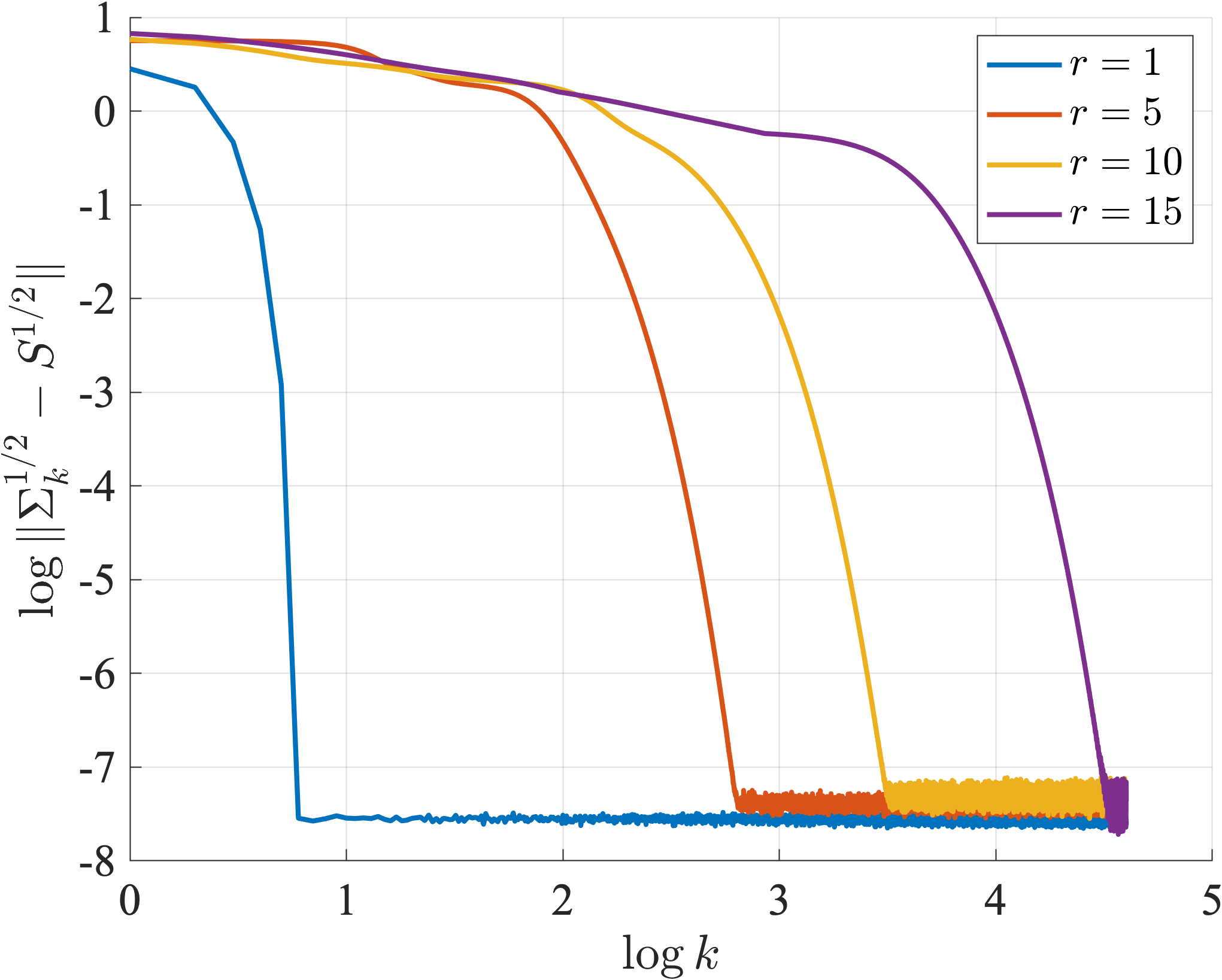
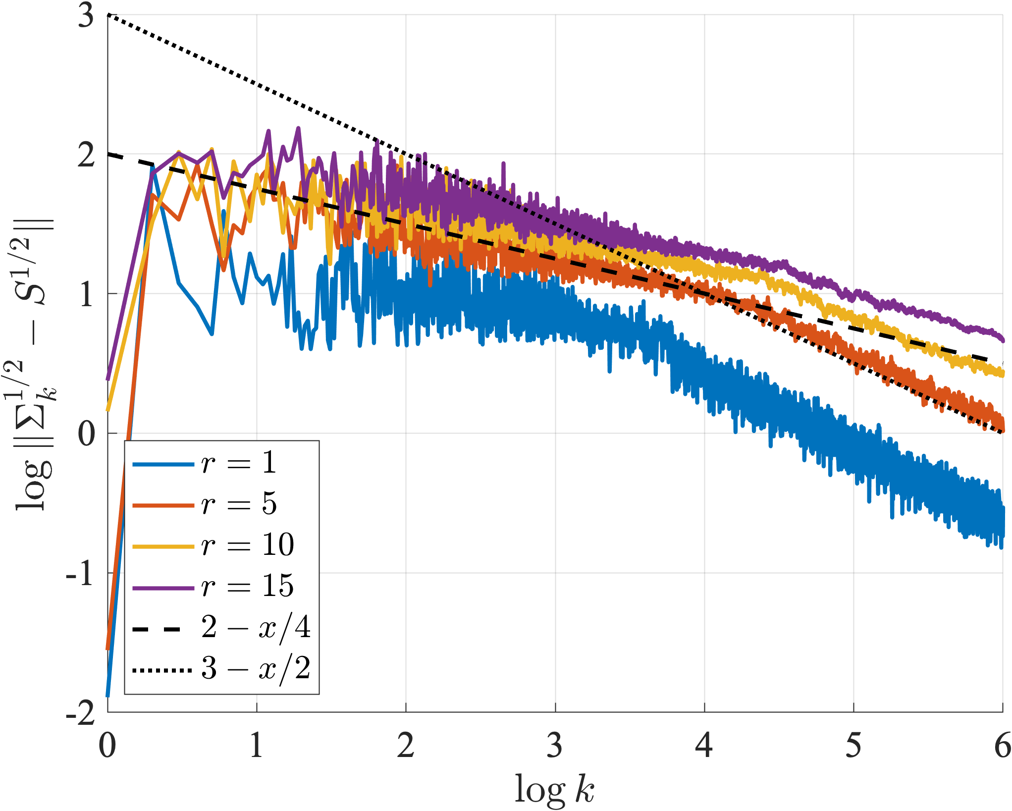
Figure 7: Convergence of BWGD and BWSGD for varying ranks.

In the plot for SGD, we also give lines to show the different rates. Here, it appears that SGD is converging to the true barycenter. Also, it appears to be converging at a faster than anticipated rate. An explanation of this phenomenon will be explored in future work. In the left plot of Figure 7, we set $d=20$ and $n=d^{2}$, and we plot the error versus iteration for BW gradient descent for the various ranks. As we can see, the convergence takes longer as the rank increases. In the right plot of Figure 7, we plot the error versus iteration for BWSGD using the single sample gradient of (2.13), where at each iteration we draw a new sample. As we can see, the BWSGD interpolates between two convergence regimes: a slow regime where the rate is $k^{-1/4}$ and a fast regime where the rate is $k^{-1/2}$. The latter rate is typical of cases where there is local strong convexity or a Polyak-Łojasiewicz inequality.

C.2 Abalone Dataset

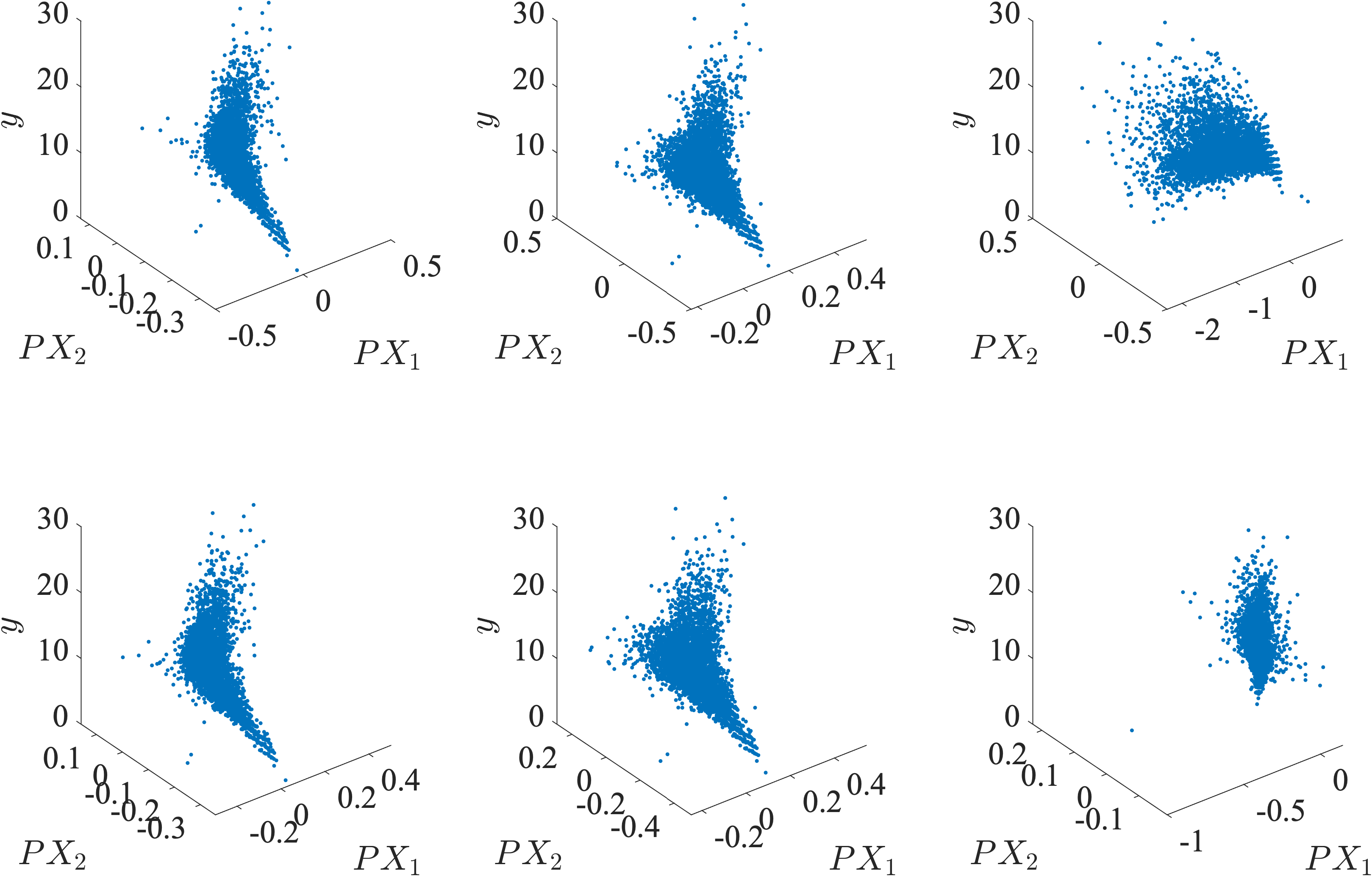
Figure 8: Projections for abalone data. The left column are projections for a fixed rank BW and full-rank BW barycenter, the middle column corresponds to low-rank and full-rank Euclidean gradient descent on (2.2), and the right column corresponds to the top principal subspace of $\boldsymbol{x}$ and the result of the spectral method.

We also present an experiment with real data. This example is one where we attempt to measure the heterogeneity in a regression dataset. Here, we pick the classical Abalone dataset available from the UCI machine learning repository [Blake and Merz, 1998]. In this dataset, one attempts to predict the age of abalone from certain covariates. Linear regression models exhibit poor fit on this data for a variety of reasons. One reason, which we demonstrate here, is the presence of heterogeneity in the measurements.

Assuming the covariance recovery model $y_{i}=\langle\boldsymbol{x}_{i},\boldsymbol{w}_{i}\rangle+\epsilon_{i},$ where $\boldsymbol{w}_{i}\sim N(\boldsymbol{0},\boldsymbol{S})$, we could try to measure heterogeneity in the data by recovering the covariance of the regression vectors, and then plotting how $\boldsymbol{x}$ relates to $y$ in its top principal space. Here, we recover such a covariance, and then project $\boldsymbol{x}$ onto the top two principal directions. We then plot $y$ against these two directions. The resulting plots show varying degrees of heterogenity depending on the method employed. Here, we compare BW gradient descent, GD, PCA on the $\boldsymbol{x}$’s, and the spectral method, which finds the top principal directions of the matrix

$$S_{n}=\frac{1}{2n}\sum_{i=1}^{n}y_{i}(\boldsymbol{x}_{i}\boldsymbol{x}_{i}^{\top}-\boldsymbol{I})$$ (C.1)

As we can see, the spectral methods completely fails here. The BW gradient descent method gives a similar but qualitatively different result from the Euclidean gradient descent method. In particular, there appear to be two primary directions of variation, which would indicate that this may be a mixture of two different regression components. Both BW gradient descent and GD recover a stretched direction, but the secondary direction (in the $PX_{1}$ direction) appears to be more pronounced for BW gradient descent.

References

- Agueh and Carlier [2011] Martial Agueh and Guillaume Carlier. Barycenters in the Wasserstein space. SIAM J. Math. Anal., 43(2):904–924, 2011.
- Altschuler et al. [2021] Jason Altschuler, Sinho Chewi, Patrik R Gerber, and Austin Stromme. Averaging on the bures-wasserstein manifold: dimension-free convergence of gradient descent. Advances in Neural Information Processing Systems, 34:22132–22145, 2021.
- Álvarez-Esteban et al. [2016] Pedro C Álvarez-Esteban, E Del Barrio, JA Cuesta-Albertos, and C Matrán. A fixed-point approach to barycenters in wasserstein space. Journal of Mathematical Analysis and Applications, 441(2):744–762, 2016.
- Ambrosio et al. [2008] Luigi Ambrosio, Nicola Gigli, and Giuseppe Savaré. Gradient flows in metric spaces and in the space of probability measures. Lectures in Mathematics ETH Zürich. Birkhäuser Verlag, Basel, second edition, 2008.
- Bhatia et al. [2019] Rajendra Bhatia, Tanvi Jain, and Yongdo Lim. On the Bures–Wasserstein distance between positive definite matrices. Expo. Math., 37(2):165–191, 2019.
- Blake and Merz [1998] C. L. Blake and C. J. Merz. UCI repository of machine learning databases, 1998. URL https://archive.ics.uci.edu/ml/datasets/abalone.
- Burer and Monteiro [2003] Samuel Burer and Renato DC Monteiro. A nonlinear programming algorithm for solving semidefinite programs via low-rank factorization. Mathematical Programming, 95(2):329–357, 2003.
- Bures [1969] Donald Bures. An extension of Kakutani’s theorem on infinite product measures to the tensor product of semifinite w*-algebras. Transactions of the American Mathematical Society, 135:199–212, 1969.
- Cai and Zhang [2015] T Tony Cai and Anru Zhang. Rop: Matrix recovery via rank-one projections. The Annals of Statistics, 43(1):102–138, 2015.
- Candès and Plan [2010] Emmanuel J Candès and Yaniv Plan. Matrix completion with noise. Proceedings of the IEEE, 98(6):925–936, 2010.
- Candès and Recht [2009] Emmanuel J Candès and Benjamin Recht. Exact matrix completion via convex optimization. Foundations of Computational mathematics, 9(6):717–772, 2009.
- Candès and Tao [2010] Emmanuel J Candès and Terence Tao. The power of convex relaxation: Near-optimal matrix completion. IEEE Transactions on Information Theory, 56(5):2053–2080, 2010.
- Candès et al. [2006] Emmanuel J Candès, Justin Romberg, and Terence Tao. Robust uncertainty principles: Exact signal reconstruction from highly incomplete frequency information. IEEE Transactions on information theory, 52(2):489–509, 2006.
- Candès et al. [2011] Emmanuel J Candès, Xiaodong Li, Yi Ma, and John Wright. Robust principal component analysis? Journal of the ACM (JACM), 58(3):1–37, 2011.
- Candès et al. [2013] Emmanuel J Candès, Thomas Strohmer, and Vladislav Voroninski. Phaselift: Exact and stable signal recovery from magnitude measurements via convex programming. Communications on Pure and Applied Mathematics, 66(8):1241–1274, 2013.
- Candès et al. [2015] Emmanuel J Candès, Yonina C Eldar, Thomas Strohmer, and Vladislav Voroninski. Phase retrieval via matrix completion. SIAM review, 57(2):225–251, 2015.
- Chandrasekaran et al. [2009] Venkat Chandrasekaran, Sujay Sanghavi, Pablo A Parrilo, and Alan S Willsky. Sparse and low-rank matrix decompositions. IFAC Proceedings Volumes, 42(10):1493–1498, 2009.
- Chen et al. [2015] Yuxin Chen, Yuejie Chi, and Andrea J Goldsmith. Exact and stable covariance estimation from quadratic sampling via convex programming. IEEE Transactions on Information Theory, 61(7):4034–4059, 2015.
- Chewi et al. [2020] Sinho Chewi, Tyler Maunu, Philippe Rigollet, and Austin J Stromme. Gradient descent algorithms for bures-wasserstein barycenters. In Conference on Learning Theory, pages 1276–1304. PMLR, 2020.
- Chi et al. [2019] Yuejie Chi, Yue M Lu, and Yuxin Chen. Nonconvex optimization meets low-rank matrix factorization: An overview. IEEE Transactions on Signal Processing, 67(20):5239–5269, 2019.
- Clarke [1990] Frank H Clarke. Optimization and nonsmooth analysis. SIAM, 1990.
- De Veaux [1989] Richard D De Veaux. Mixtures of linear regressions. Computational Statistics & Data Analysis, 8(3):227–245, 1989.
- Diakonikolas et al. [2019] Ilias Diakonikolas, Gautam Kamath, Daniel Kane, Jerry Li, Ankur Moitra, and Alistair Stewart. Robust estimators in high-dimensions without the computational intractability. SIAM Journal on Computing, 48(2):742–864, 2019.
- Donoho [2006] David L Donoho. Compressed sensing. IEEE Transactions on information theory, 52(4):1289–1306, 2006.
- Du et al. [2019] Simon Du, Jason Lee, Haochuan Li, Liwei Wang, and Xiyu Zhai. Gradient descent finds global minima of deep neural networks. In International conference on machine learning, pages 1675–1685. PMLR, 2019.
- Fazel [2002] Maryam Fazel. Matrix rank minimization with applications. PhD thesis, PhD thesis, Stanford University, 2002.
- Fienup [1978] James R Fienup. Reconstruction of an object from the modulus of its fourier transform. Optics letters, 3(1):27–29, 1978.
- Ghadimi and Lan [2013] Saeed Ghadimi and Guanghui Lan. Stochastic first-and zeroth-order methods for nonconvex stochastic programming. SIAM Journal on Optimization, 23(4):2341–2368, 2013.
- Gross et al. [2010] David Gross, Yi-Kai Liu, Steven T Flammia, Stephen Becker, and Jens Eisert. Quantum state tomography via compressed sensing. Physical review letters, 105(15):150401, 2010.
- Hotelling [1933] Harold Hotelling. Analysis of a complex of statistical variables into principal components. Journal of educational psychology, 24(6):417, 1933.
- Knott and Smith [1994] Martin Knott and Cyril S Smith. On a generalization of cyclic monotonicity and distances among random vectors. Linear algebra and its applications, 199:363–371, 1994.
- Lerman and Maunu [2018] Gilad Lerman and Tyler Maunu. An overview of robust subspace recovery. Proceedings of the IEEE, 106(8):1380–1410, 2018.
- Li et al. [2019] Yuanxin Li, Cong Ma, Yuxin Chen, and Yuejie Chi. Nonconvex matrix factorization from rank-one measurements. In The 22nd International Conference on Artificial Intelligence and Statistics, pages 1496–1505. PMLR, 2019.
- Massart and Absil [2020] Estelle Massart and P-A Absil. Quotient geometry with simple geodesics for the manifold of fixed-rank positive-semidefinite matrices. SIAM Journal on Matrix Analysis and Applications, 41(1):171–198, 2020.
- Nesterov [2004] Yurii Nesterov. Introductory lectures on convex optimization: A basic course, volume 87. Springer Science & Business Media, 2004.
- Pearson [1901] Karl Pearson. Liii. on lines and planes of closest fit to systems of points in space. The London, Edinburgh, and Dublin philosophical magazine and journal of science, 2(11):559–572, 1901.
- Recht et al. [2010] Benjamin Recht, Maryam Fazel, and Pablo A Parrilo. Guaranteed minimum-rank solutions of linear matrix equations via nuclear norm minimization. SIAM review, 52(3):471–501, 2010.
- Sanghavi et al. [2017] Sujay Sanghavi, Rachel Ward, and Chris D White. The local convexity of solving systems of quadratic equations. Results in Mathematics, 71(3):569–608, 2017.
- Sedghi et al. [2016] Hanie Sedghi, Majid Janzamin, and Anima Anandkumar. Provable tensor methods for learning mixtures of generalized linear models. In Artificial Intelligence and Statistics, pages 1223–1231. PMLR, 2016.
- Tu et al. [2016] Stephen Tu, Ross Boczar, Max Simchowitz, Mahdi Soltanolkotabi, and Ben Recht. Low-rank solutions of linear matrix equations via procrustes flow. In International Conference on Machine Learning, pages 964–973. PMLR, 2016.
- Villani [2009] Cédric Villani. Optimal transport: old and new, volume 338 of Grundlehren der Mathematischen Wissenschaften [Fundamental Principles of Mathematical Sciences]. Springer-Verlag, Berlin, 2009.
- Wang and Giannakis [2016] Gang Wang and Georgios Giannakis. Solving random systems of quadratic equations via truncated generalized gradient flow. Advances in Neural Information Processing Systems, 29, 2016.
- Wang et al. [2017] Gang Wang, Georgios Giannakis, Yousef Saad, and Jie Chen. Solving most systems of random quadratic equations. Advances in Neural Information Processing Systems, 30, 2017.
- Xu et al. [2010] Huan Xu, Constantine Caramanis, and Sujay Sanghavi. Robust pca via outlier pursuit. Advances in neural information processing systems, 23, 2010.
- Yi et al. [2014] Xinyang Yi, Constantine Caramanis, and Sujay Sanghavi. Alternating minimization for mixed linear regression. In International Conference on Machine Learning, pages 613–621. PMLR, 2014.
- Zemel and Panaretos [2019] Yoav Zemel and Victor M. Panaretos. Fréchet means and Procrustes analysis in Wasserstein space. Bernoulli, 25(2):932–976, 2019.
- Zhang and Sra [2016] Hongyi Zhang and Suvrit Sra. First-order methods for geodesically convex optimization. In 29th Annual Conference on Learning Theory, volume 49 of Proceedings of Machine Learning Research, pages 1617–1638, Columbia University, New York, New York, USA, 2016.
- Zhong et al. [2015] Kai Zhong, Prateek Jain, and Inderjit S Dhillon. Efficient matrix sensing using rank-1 gaussian measurements. In International conference on algorithmic learning theory, pages 3–18. Springer, 2015.
- Zhong et al. [2016] Kai Zhong, Prateek Jain, and Inderjit S Dhillon. Mixed linear regression with multiple components. In NIPS, pages 2190–2198, 2016.
- Zhong et al. [2017] Kai Zhong, Zhao Song, Prateek Jain, Peter L Bartlett, and Inderjit S Dhillon. Recovery guarantees for one-hidden-layer neural networks. In International conference on machine learning, pages 4140–4149. PMLR, 2017.