Boosting Semi-Supervised Semantic Segmentation with Probabilistic Representations
Abstract
Recent breakthroughs in semi-supervised semantic segmentation have been developed through contrastive learning. In prevalent pixel-wise contrastive learning solutions, the model maps pixels to deterministic representations and regularizes them in the latent space. However, there exist inaccurate pseudo-labels which map the ambiguous representations of pixels to the wrong classes due to the limited cognitive ability of the model. In this paper, we define pixel-wise representations from a new perspective of probability theory and propose a Probabilistic Representation Contrastive Learning (PRCL) framework that improves representation quality by taking its probability into consideration. Through modelling the mapping from pixels to representations as the probability via multivariate Gaussian distributions, we can tune the contribution of the ambiguous representations to tolerate the risk of inaccurate pseudo-labels. Furthermore, we define prototypes in the form of distributions, which indicates the confidence of a class, while the point prototype cannot. Moreover, we propose to regularize the distribution variance to enhance the reliability of representations. Taking advantage of these benefits, high-quality feature representations can be derived in the latent space, thereby the performance of semantic segmentation can be further improved. We conduct sufficient experiment to evaluate PRCL on Pascal VOC and CityScapes to demonstrate its superiority. The code is available at https://github.com/Haoyu-Xie/PRCL.
Introduction
Semantic segmentation is a pixel-level classification task, i.e. predicting the class of each pixel. Existing supervised methods rely on large-scale annotated data, which requires high manual-labeling costs. Semi-supervised learning (Ouali, Hudelot, and Tami 2020; Ke et al. 2020b; Zou et al. 2021; Sohn et al. 2020) takes advantage of unlabeled data and relieves the labor of human annotation. Some methods use unlabeled data to improve segmentation models via adversarial learning (Ke et al. 2020b), consistency regularization (Peng et al. 2020), and self-training (Tarvainen and Valpola 2017). Self-training is a typical solution that uses the prediction generated by a model trained on labeled data (called pseudo-label) as ground-truth to train unlabeled data.
Recently, powerful methods based on self-training (Liu et al. 2021; Wang et al. 2022) additionally introduce a pixel-wise contrastive learning as an auxiliary task to further explore unlabeled data. Contrastive learning benefits from not only the local context of neighbouring pixels, but also global semantic class relations across the mini-batch even the entire dataset. They map pixels to representations and regularize them in the latent space in a supervised way, i.e. gather representations belonging to the same class and scatter representations belonging to different classes, where the semantic class information comes from both ground truths and pseudo-labels. Most of contrastive learning methods is guided by pseudo-labels in semi-supervised settings. Therefore, the quality of pseudo-labels is critical since inaccurate pseudo-labels lead to assigning representations to wrong classes and cause a disorder in latent space. Existing efforts try to polish pseudo-labels via either confidence (Liu et al. 2021) or entropy (Feng et al. 2022). These techniques can improve the quality of pseudo-labels and eliminate inaccurate ones to some extent. However, the inherent noise as well as essential incorrectness in pseudo-labels are rather difficult to be perfectly tackled by existing work. Thus, we propose to alleviate this risk in an opposite way. Specifically, instead of paying more attention to polishing pseudo-labels for inaccuracy elimination, we propose to improve the quality of representations from data via modelling probability, and allow them to perform better under the inaccurate pseudo labels.
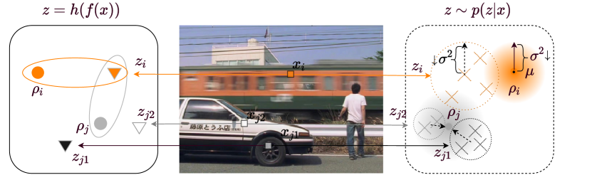
Comparing with existing conventional deterministic representation modelling, we model representations as a random variable with learnable parameters and represent prototypes in the form of distributions. We take the form of multivariate Gaussian distribution for both representations and prototypes. An illustration of proposed probabilistic representations and distribution prototypes is shown in Figure 1. The involvement of probability is shown in . The pixel of the fuzzy train carriage is mapped to in the latent space which contains two parts including the most like representation and the probability which correspond to the mean and variance of distribution respectively. Similarly, the pixels of the car and are mapped to and respectively. For comparison, deterministic mapping is shown in . Considering the scenario where the distance from representation to prototype is same as the distance from to , there exist an ambiguity of the mapping from to and in deterministic representation. On the contrary, is mapped to in probabilistic representation since has a smaller than . Note that is inversely proportional to the probability, which implies that the mapping from to is more reliable. Furthermore, and contribute to the car prototype to different degrees. Through taking the probability of representations into consideration, the prototypes can be estimated more accurately. Meanwhile, the variance is constrained during the training procedure, which further improves the reliability of the representations and prototypes.
In this paper, we define pixel-wise representations and prototypes from a new perspective of probability theory and design a new framework for pixel-wise Probabilistic Representation Contrastive Learning, named PRCL. Our key insight is to: (i) involve modelling probability into the representations and prototypes, and (ii) explore a more accurate similarity measurement between probabilistic representations and prototypes. For the first objective (i), we concatenate an Probability head (Multilayer Perceptron, MLP) to encoder to predict the probabilities of representations and construct a distribution prototype with probabilistic representations as observations based on Bayesian Estimation (Vaseghi 2008). In the latent space, each prototype is represented as a distribution rather than a point, which enables them to explore the uncertainty. For objective (ii), we leverage mutual likelihood score (MLS) (Shi and Jain 2019) to directly compute the similarity among probabilistic representations and distribution prototypes. MLS can naturally adjust the weight of distance based on the uncertainty, i.e. penalize ambiguous representations and vice versa. Taking the advantage of the confidence information contained in probabilistic representations, model robustness to inaccurate pseudo-labels is significantly enhaned for stable training. In addition, we propose a soft freezing strategy to optimize probability head free from probability converging sharply to during training without constraint.
In summary, we propose to alleviate the negative effects from inaccurate pseudo-labels by introducing probabilistic representation with PRCL framework, which reduces the contribution of representations with high uncertainty and concentrates on more reliable ones in contrastive learning. To the best of our knowledge, we are the first to simultaneously train the representation and probability. Extensive evaluation on Pascal VOC (Everingham et al. 2010) and CityScapes (Cordts et al. 2016) to demonstrate the superior performances than the SOTA baselines.
Related Work
Semi-supervised semantic segmentation
The goal of semantic segmentation is to classify each pixel in an entire image by class. The training of such dense prediction tasks relies on large amounts of data and tedious manual annotations. Semi-supervised learning is a label-efficient task that needs to take advantage of a large amount of unlabeled data to improve model performance. Entropy minimization (Hung et al. 2018; Ke et al. 2020a) and consistency regularization (Ouali, Hudelot, and Tami 2020; Peng et al. 2020; Fan et al. 2022) are two main branches. Recently, self-training methods benefit from strong data augmentation (French et al. 2020; Olsson et al. 2021; Hu et al. 2021) and well-refined pseudo-labels (Sohn et al. 2020; Feng et al. 2022). Besides, some methods (Guan et al. 2022) balancing the distributions of subclass are competitive in some scenarios. Recent works based on self-training (Liu et al. 2021; Wang et al. 2022; Xie et al. 2022) attempt to regularize representations in latent space for better embedding space distribution. This improves the quality of features and leads to better model performance, which is also our goal.
Contrastive Learning
As a major branch of metric learning, the key idea of contrastive learning is to pull positive pairs close and push negative pairs apart in the latent feature space through a contrastive loss. At the instance level, it treats each image as a single class and distinguishes the image from others in multiple views (Wu et al. 2018; Ye et al. 2019; Chen et al. 2020; He et al. 2020; Grill et al. 2020). To alleviate the negative impact of sampling bias, some works (Chuang et al. 2020) try to correct for the sampling of same-label data, even without the information of true labels. Furthermore, in some supervised or semi-supervised settings, some works (Zhao et al. 2022) introduce class information to train models to distinguish between classes. At the pixel level, pixel-wise representations are distinguished by labels or pseudo-labels (Lai et al. 2021; Wang et al. 2021). However, in the semi-supervised setting, only a small amount of labeled data is available. Most pixel divisions are based on pseudo-labels, and inaccurate pseudo-labels lead to a disorder in the latent space. To address these issues, previous methods (Liu et al. 2021; Alonso et al. 2021) try to polish pseudo-labels. In our approach, we focus on tolerating inaccurate pseudo-labels rather than filtering them.
Probabilistic Embedding
Probabilistic Embeddings (PE) is an extension of conventional embeddings. Methods of PE usually predict the overall distribution of the embeddings, e.g. , Gaussian (Shi and Jain 2019) and von Mises-Fisher (Li et al. 2021), rather than a single vector. The ability of neural networks to predict distributions stems from the work of Mixture Density Networks (MDN) (Bishop 1994). Later, Variable Auto-Encoders (VAE) (Kingma and Welling 2013) first proposed the use of MLP to predict the mean and variance of a distribution. Most of works on probabilistic embeddings (Shi and Jain 2019; Scott, Ridgeway, and Mozer 2019; Scott, Gallagher, and Mozer 2021; Park et al. 2022) are based on this architecture. Hedged Instance emBeddings (HIB) (Oh et al. 2019) is the first attempt to apply PE to image retrieval and verifications. Further, PE is applied to face verification tasks. In Probabilistic Face Embeddings (PFE) (Shi and Jain 2019), each image is mapped to a Gaussian distribution in the latent space, with the mean produced by a pre-trained model and variance predicted via an MLP (some works call it uncertainty head, we name it probability head in our work). And Sphere Confidence Face (SCF) (Li et al. 2021) maps image to a von Mises-Fisher distribution with mean and concentration parameter. We borrow the same architecture, but it is worth noting that PFE and SCF optimize mean and variance (concentration parameter) in two stages, i.e. pre-train a deterministic model to predict the mean and freeze it to optimize the variance. But in our work, the mean and variance are optimized simultaneously, which allows them to interact with each other.
Although the conventional distance metric can measure the similarity of distribution using their mean, it is insufficient to represent the probabilistic similarity due to variance. To address this issue, HIB uses the reparameter trick (Kingma and Welling 2013) to obtain two sets of samples from two distributions through Monte-Carlo sampling, and accumulates the similarity of samples to represent the distribution similarity. PFE and SCF directly compute distribution similarity using mutual likelihood score, but they can not simultaneously optimize mean and variance. This is because uncertainty/probability (variance) is only valuable if representation (mean) is reasonable. PFE and SCF achieve this by training the mean and variance in two stages, and we address this by training them separately with different learning rates.
Methodology
Preliminaries
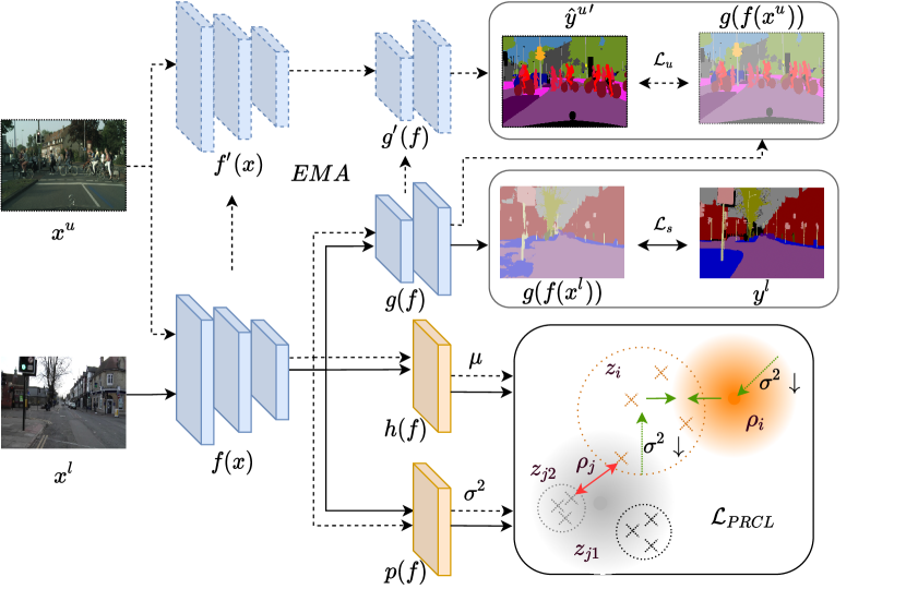
The objective of semi-supervised semantic segmentation is to train a model with only a limited amount of labeled data and substantial unlabeled data . An illustration of our framework is shown in Figure 2. Following the typical self-training frameworks, our framework consists of two networks with the same architecture, named student network and teacher network respectively. Each model contains an encoder and a predictor . We denote , as the encoder and predictor of student network and , as those of teacher network. The student network parameters are optimized via stochastic gradient descent (SGD) to minimize the loss function while the teacher network parameters are updated by Exponential Moving Average (EMA) of the student network parameters. In addition, in contrastive learning-based semi-supervised methods, a representation head is introduced to student network to map pixels to representations and a contrastive loss is computed between them. For simplicity, we denote the one hot coding format of the pseudo-label from teacher network as and the projection result as . A supervised cross entropy loss is calculated between the prediction of student network and ground truth . And an unsupervised cross entropy loss is calculated between the prediction of the student network and the pseudo-label from teacher network. The overall loss for contrastive learning-based semi-supervised segmentation is formulated as
|
|
(1) |
|
|
|
|
where and are two hyper-parameters to adjust the contributions of and respectively, and and denote labeled images and unlabeled images in a mini-batch respectively. The contrastve learning loss is computed by infoNCE (Van den Oord, Li, and Vinyals 2018) as follows:
|
|
(2) |
where denotes the set including all available classes in a mini-batch, denotes the set including sampled anchor representations belonging to anchor class , denotes the set of classes other than , denotes the set including sampled negative representations belonging to class , denotes the temperature control of the softness of the distribution, and denotes similarity measurement, e.g., cosine similarity and distance, in our work, mutual likelihood score (MLS) (Shi and Jain 2019) is leveraged. In addition, are representations mapped from the pixels belonging to the same class , and the class information is obtained from labels of labeled data and pseudo-labels of unlabeled data. The goal of contrastive learning is to improve the representation capability of the encoder by regularizing the representations for the better performance in the downstream semantic segmentation tasks. Considering an ideal representation space for downstream tasks, the similar representations of the same class are concentrated around the corresponding prototype , while the prototypes of different classes should be separated from each other. However, due to inaccurate pseudo-labels, there is a mismatch between and . Our goal is to further improve the representation performance for the robustness under this case.
Probabilistic Representation
The representations in conventional contrastive learning are deterministic. However, there exist inaccurate pseudo-labels which map the ambiguous representations of pixels to the wrong classes due to the limited cognitive ability of the model. Concretely, some pixels from the class will be treated as one of another classes , leading to a perturbation in calculating. Although it is difficult to perform complete elimination of inaccurate pseudo-labels, we can model the mapping probability to measure its confidence, thereby reducing low confidence mapping caused by inaccurate pseudo-labels. We denote the probability of mapping a pixel to a representation as and define the representation as a random variable following it. For simplicity, we take the form of multivariate Gaussian distribution as
| (3) |
where represents the unit diagonal matrix. In this form, can be viewed as most like representation values, and can show the probability in the representation values. It is worth noting that is inversely proportional to probability, i.e. the greater the , the lower the probability, which is consistent with the form in MLS. Both dimensions of and are the same. The mean is predicted by the representation head . Meanwhile, we introduce a probability head in parallel to predict the variance , as shown in Figure 2. To achieve the better representation learning for downstream semantic segmentation tasks, the same class representations should concentrate on their prototypes in the latent space. The prototype can be calculated with the mean of the same class representations in deterministic representation methods as
| (4) |
where is the number of representations sampled. This method has a limitation that all representations contribute the same to the prototype. In our method, instead, we estimate it using Bayesian Estimation incorporating new probabilistic representations as observations. With probabilistic representations, a conjugate formula can be derived for prototype estimation. The prototype is the posterior distribution after the observations . Under the assumption that all the observations are conditionally independent, the distribution prototype can be derived as
|
|
(5) |
where is a normalization factor. In addition to Equation 3, we can rewrite the prototype as
| (6) |
where
| (7) |
| (8) |
From the Equation 7, we can know that the representations with different probabilities contribute differently to the prototype. The smaller (higher probability) corresponds to more contribution, and vice versa. And the negative impact of high-risk false representations will be reduced, so the prototypes can be estimated reliably. And with the , the distribution prototype act as a radius region in the latent space, which can express the potential location of the exact prototype with probability. As Equation 8 shows, during the training, with more representations accumulation, the of prototype decreases. The region of distribution prototype becomes smaller. In other words, the estimated prototype becomes clearer. Proof details refer to (Shi and Jain 2019).
Probabilistic Representation Contrastive Learning
According to the previous section, we redefine and in Equation 2. However, conventional distance does not have the ability to measure the similarity between two distributions. To solve this problem, we leverage the Mutual likelihood Score (MLS) to measure the similarity between two distributions and , as follows:
|
|
(9) |
where refers to the dimension of and the same for . MLS is a combination of a weighted distance and a log regularization term, essentially. Conventional distance only consider the similarity between representations mapped in the latent space by the pseudo-labels without considering their reliability. The inaccurate pseudo-labels leads to a wrong optimizing direction, which destructs the latent space. We argue that inaccurate pseudo-labels often come with the low probabilities. With probabilities of and , MLS responds to inaccurate pseudo-labels from two perspectives. (i): In the first term, the weight of distance is small when the is large, which indicates that the similarity between and becomes lower due to the low probabilities, even if they are very similar in the view of distance. The probability has been taken into consideration besides the simple similarity measure for representations learning. (ii): In the second term, is penalized for the low probability representations, which makes all the representations more reliable. Besides, and can interact with each other. The learnable is associated with distance. This means that can be learned via the relations among representations. On the other hand, the can also be optimized via the . This is consistent with intuitive cognition.
We introduce Equation 9 into Equation 2 and rewrite it as
|
|
(10) |
and name it PRCL loss , whose pseudo-code is shown in Appendix A. Like conventional contrastive learning, the negatives push each other away, while the positives converge toward the prototype. In addition, optimized with the PRCL loss, the of probabilistic representations on a downward trend, i.e. the representations get more and more certain. With the accumulation of representations, the of prototypes are decreasing, i.e. the prototype becomes clearer, which is verified in our empirical evaluation of their tendency during training in Experiment Section. And we apply PRCL loss to both labeled and unlabeled data. Cooperated with supervised cross-entropy loss and unsupervised cross-entropy loss , the overall loss for semi-supervised segmentation is rewrited as
| (11) |
In , we only consider the pixels whose predicted confidence (the maximum of prediction after SoftMax operation) are greater than , and is defined as the percentage of them, following the prior method (Olsson et al. 2021). is a time-variant scaling parameter to control the weight of . We refer more details to the Experiment Section.
Soft Freezing
We find optimization instability where would converge to if left unbounded. At the beginning of training, the probability head output increases substantially, causing training to crash. We mainly attribute it to the fact that the representations is unreasonable at the beginning of the training. At this stage, optimizing probability with unreasonable representations is meaningless. It is crucial to use some empirical tricks to avoid it. Some works (Shi and Jain 2019; Li et al. 2021) freeze the trained representation head when training probability head. Some works pre-train the representations and freeze it when training probability head freezing the trained representations later. In addition, an additional KL regularization term between the distribution and the unit Gaussian prior is employed to prevent the from converging to . However, intuitively, this trick will hinder the interaction between probability and representation, thus limiting the performance of the probability. To address this issue, we separate the training of the probability head from the ensemble and train it with a much smaller learning rate in our work. This makes probability head training keep pace with others for stable optimization and enables simultaneous training of the probability and the representation to interact with each other. We name this empirical trick Soft Freezing.
Experiments
Dataset. We conduct experiments on Pascal VOC 2012 (Everingham et al. 2010) dataset and CityScapes (Cordts et al. 2016) dataset to test the effectiveness of PRCL. The Pascal VOC 2012 contains 1464 well-annotated images for training and 1449 images for validation originally. Following (Liu et al. 2021; Wang et al. 2022; Yang et al. 2022), we introduce SBD (Hariharan et al. 2011) as additional training data into training set. CityScapes is an urban scene dataset which includes 2975 training images and 500 validation images.
Network structure. We use DeepLabv3+ (Chen et al. 2018) with ResNet-101 (He et al. 2016) pre-trained on ImageNet (Deng et al. 2009). The prediction head and representation head are composed of Conv-BN-ReLU-Conv. The probability head is composed of Linear-BN-ReLU-Linear-BN.
Sampling strategy. Due to limited computation and memory, it would be unachievable for us to sample all pixels in the training set. In our method, we follow the prior work (Liu et al. 2021) and adopt some sampling strategies. (a) Valid samples sampling strategy: In order to artificially avoid some noise and refine more meaningful representations, we set a threshold for sampling valid representations. Representations will be valid only if its corresponding is higher than . (b) Anchor sampling strategy: For the purpose of paying more attention to relatively ambiguous representations, we set a threshold for and randomly sample a suitable number of hard anchors whose are below , which makes our training focus on the ambiguous representations. (c) Negative samples sampling strategy: We non-uniformly sample a suitable number of negative representations for each anchor. The sampling ratio is based on the similarity between prototype for negative representation classes and that for current anchor class .
Experimental details. We adjust PRCL contribution with a loss scheduler. Mathematically, given the total training epochs and the initial weight , the weight at the -th epoch can be calculated as,
| (12) |
where is a negative constant, which determines the rate of weight descent.
Evaluation. We adopt the mean of Intersection over Union (mIoU) as the metric to evaluate the performance of our work. All results are measured on the val set in both Pascal VOC and CityScapes.
Probability Behavior
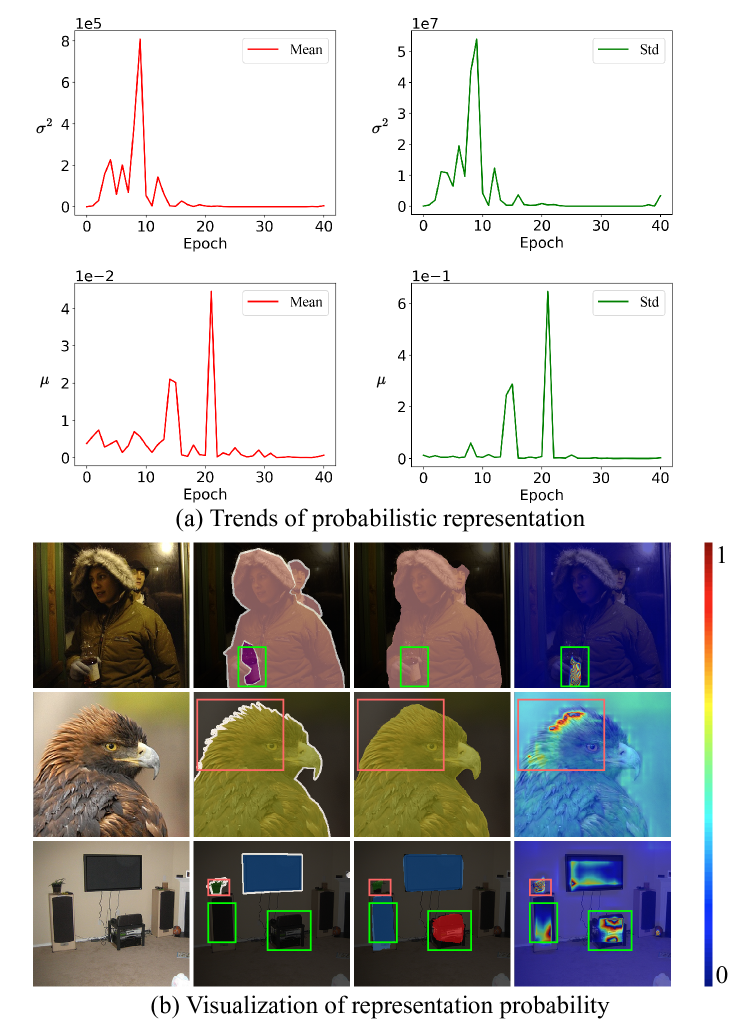
Figure 3 shows the behavior of the probability (The norm of ) and reflects the relationship between probability and inaccurate pseudo-labels. In Figure 3(a), first row represents the mean and standard deviation of in representation during training, and second row represents the same statistics of . At the beginning of training process, representations are unreasonable, which lead to a large . When representations are more and more certain, is decreasing and is more meaningful. In Figure 3(b), columns from left to right represent input image, ground-truth, pseudo-label, and probability, respectively. For the fourth column, the red color represents the large (low probability). The green boxes mark the mismatches caused by inaccurate pseudo-labels (e.g., person and bottle) and the red boxes mark the fuzzy pixels (e.g., furry edge of the bird). These two cases are highlighted by and make low contribution in training process.
Comparison with Existing Methods
In this subsection, firstly, we reproduce two semi-supervised segmentation baselines: Mean Teacher (MT) and ClassMix (Olsson et al. 2021) on Pascal VOC and CityScapes. In addition, we also conduct the experiment only on labeled dataset (Supervised) to demonstrate our effective use of abundant unlabeled data. These methods are conducted with standard DeepLabv3+ and ResNet-101 under the same settings. Besides, for fair comparing, we use the modified ResNet-101 with the deep stem block as our backbone to compare with state-of-the-art methods, following previous works (Chen et al. 2021; Wang et al. 2022; Yang et al. 2022). In addition, our labeled dataset splits are also derived from the previous work (Wang et al. 2022; Yang et al. 2022; Liu et al. 2022).
| Pascal VOC | |||
|---|---|---|---|
| Method | labels | labels | labels |
| Supervised | |||
| MT | |||
| ClassMix | |||
| PRCL(w/ClassMix) | |||
| CityScapes | |||
|---|---|---|---|
| Method | labels | labels | labels |
| Supervised | |||
| MT | |||
| ClassMix | |||
| PRCL(w/ClassMix) | |||
Results on Pascal VOC. Table 1 shows the results of the comparison among our work and baselines on Pascal VOC. PRCL consistently outperforms other methods at all label rates in our experiment setting. Notably, our PRCL framework can improve the performance in very limited data situations, where the performance improvement is more meaningful in a semi-supervised setting.
Results on CityScapes. Table 2 illustrates the results of comparison among our work and baselines on CityScapes. PRCL achieves a marginal out-performance over all baselines across a wide range of the number of labeled images. Similar with the result on Pascal VOC, our framework can unlock more potential in low label rate.
| Pascal VOC | |||||
| Method | 92 | 183 | 366 | 662 | |
| Supervised | |||||
| PseudoSeg(w/ CutOut) | - | ||||
| CPS(w/ CutMix) | |||||
| PC2Seg(w/ CutOut) | - | ||||
| U2PL(w/ CutMix) | |||||
| ST++(w/ CutOut) | |||||
| PSMT | - | ||||
| PRCL(w/ ClassMix) | |||||
| Fully-supervised setting (10582 images): 78.20 | |||||
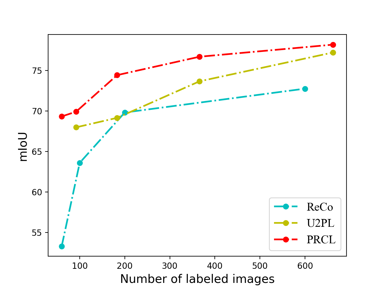
Comparison with SOTAs. We compare our work with following recent SOTAs with their own strong data augmentations (CutOut, CutMix, and ClassMix): PseudoSeg (Zou et al. 2021), CPS (Chen et al. 2021), PC2Seg (Zhong et al. 2021), PSMT (Liu et al. 2022), U2PL (Wang et al. 2022), ST++ (Yang et al. 2022), and ReCo (Liu et al. 2021) on Pascal VOC dataset. Table 3 shows the result. Our PRCL performs better than other works, especially in the scenarios with low label rates. Similar works based on pixel-wise contrastive learning (Liu et al. 2021; Wang et al. 2022) focus on polishing pseudo-labels to pick the correct representation. Instead, we focus on improving the quality of represetations for robustness under inaccurate pseudo-labels. The results are shown in Figure 4.
Ablation Study
We conduct the ablation studies based on DeepLabV3+ and ResNet-101 on Pascal VOC. And all the labeled images are the same as above experiments.
| 60 labels | 92 labels | |||
|---|---|---|---|---|
| w/o P | ||||
| w/ P | ||||
Impact of probabilistic representation and distribution prototype. To examine the effectiveness of probabilistic mechanism, we compare with deterministic representations and point prototypes. And we choose distance as a similarity measurement of them. In addition, to demonstrate the robustness to high-risk false representations, we adjust the strong threshold to vary the proportion of unconfident samples. To amplify the effect of the PRCL loss, we conduct experiments without loss scheduler. Tabel 4 shows the result on 2 label rates. We observe that under the same settings, our algorithm with probabilistic mechanism performs almost better in both two label rates. Especially, when lower the strong threshold, our framework will achieve better performance while that with deterministic representation and point prototype is hurt visibly. We mainly attribute it to the more sampled low-confident anchors with low strong threshold. We argue that there are more critical samples in low-confident predictions since the model does not fully grasp the information of corresponding pixels. It will be more efficient to concentrate on this part of pixels. However, low confidence leads to introduce more inaccurate pseudo-labels. The deterministic representations have no ability to handle these inaccurate pseudo-labels, thus leading to disorder in latent space. And this dramatically hurts the performance of semantic segmentation. With our probabilistic mechanism, the model is error-tolerant and reduces the damage to the latent space from inaccurate pseudo-labels while taking full advantage of high-risk but critical representations. In addition, we conduct the experiments without the sampling strategy ( and to demonstrate its necessity.
| Labels | 46 | 60 | 92 | 183 | 336 | 662 |
|---|---|---|---|---|---|---|
| w/o LS | ||||||
| w/ LS |
Impact of Loss scheduler. In Table 5, we evaluate the effectiveness of Loss Scheduler (LS). We can observe that with a high label rate, the model with a loss scheduler performs better than the one without a loss scheduler. However, with low label rate, model with LS performs slightly worse than model without LS. We argue that at low label rates, i.e. with less guidance, there will be more inaccurate pseudo-labels. This case will unlock the potential of probabilistic representations. Increasing the proportion of contrastive loss in total loss can promote a better distribution in latent space, which will help the downstream task. When training with a high label rate, pseudo-labels become more reliable. We should pay more attention to downstream semantic segmentation tasks and decrease the proportion of contrastive loss. Impact of negative numbers. We evaluate the performance of different number of negatives used in PRCL framework. In Table 6, we can observe that performance is better when sampling more negatives. This is because the distribution of sampled negatives is more similar with the true distribution when sample more negatives.
| Number of negatives | 64 | 128 | 256 | 512 |
|---|---|---|---|---|
| mIoU |
Conclusion
In this work, we define pixel-wise representations and prototypes from a new perspective of probability theory and design some tricks to optimize them. Probabilistic representations alleviate the negative effects from inaccurate pseudo-labels for better performance in contrastive learning. Besides, a more reliable distribution prototype can be estimated with them. Based on probabilistic representations and distribution prototypes, we propose a PRCL framework for better representation distribution to improve the performance on semi-supervised semantic segmentation tasks. Extensive experiments prove the effectiveness of PRCL and its superiority compared with other SOTAs. As Socrates said, The only true wisdom is in knowing you know nothing. Models need not only what they know, but how much they know. We hope that this simple but effective framework enables the renaissance of Bayesian theory in computer vision.
Acknowledgements
This work was supported in part by the Australian Research Council under Project DP210101859 and the University of Sydney Global Development Award (GDA). The authors acknowledge the use of the National Computational Infrastructure (NCI) which is supported by the Australian Government, and accessed through the NCI Adapter Scheme and Sydney Informatics Hub HPC Allocation Scheme.
References
- Alonso et al. (2021) Alonso, I. n.; Sabater, A.; Ferstl, D.; Montesano, L.; and Murillo, A. C. 2021. Semi-Supervised Semantic Segmentation With Pixel-Level Contrastive Learning From a Class-Wise Memory Bank. In Proceedings of the IEEE/CVF International Conference on Computer Vision (ICCV), 8219–8228.
- Bishop (1994) Bishop, C. M. 1994. Mixture density networks.
- Chen et al. (2018) Chen, L.-C.; Zhu, Y.; Papandreou, G.; Schroff, F.; and Adam, H. 2018. Encoder-decoder with atrous separable convolution for semantic image segmentation. In Proceedings of the European conference on computer vision (ECCV), 801–818.
- Chen et al. (2020) Chen, T.; Kornblith, S.; Norouzi, M.; and Hinton, G. 2020. A Simple Framework for Contrastive Learning of Visual Representations. In III, H. D.; and Singh, A., eds., Proceedings of the 37th International Conference on Machine Learning, volume 119 of Proceedings of Machine Learning Research, 1597–1607. PMLR.
- Chen et al. (2021) Chen, X.; Yuan, Y.; Zeng, G.; and Wang, J. 2021. Semi-supervised semantic segmentation with cross pseudo supervision. In Proceedings of the IEEE/CVF Conference on Computer Vision and Pattern Recognition, 2613–2622.
- Chuang et al. (2020) Chuang, C.-Y.; Robinson, J.; Lin, Y.-C.; Torralba, A.; and Jegelka, S. 2020. Debiased contrastive learning. Advances in neural information processing systems, 33: 8765–8775.
- Cordts et al. (2016) Cordts, M.; Omran, M.; Ramos, S.; Rehfeld, T.; Enzweiler, M.; Benenson, R.; Franke, U.; Roth, S.; and Schiele, B. 2016. The cityscapes dataset for semantic urban scene understanding. In Proceedings of the IEEE conference on computer vision and pattern recognition, 3213–3223.
- Deng et al. (2009) Deng, J.; Dong, W.; Socher, R.; Li, L.-J.; Li, K.; and Fei-Fei, L. 2009. Imagenet: A large-scale hierarchical image database. In 2009 IEEE conference on computer vision and pattern recognition, 248–255. Ieee.
- Everingham et al. (2010) Everingham, M.; Van Gool, L.; Williams, C. K.; Winn, J.; and Zisserman, A. 2010. The pascal visual object classes (voc) challenge. International journal of computer vision, 88(2): 303–338.
- Fan et al. (2022) Fan, J.; Gao, B.; Jin, H.; and Jiang, L. 2022. UCC: Uncertainty guided Cross-head Co-training for Semi-Supervised Semantic Segmentation. In Proceedings of the IEEE/CVF Conference on Computer Vision and Pattern Recognition, 9947–9956.
- Feng et al. (2022) Feng, Z.; Zhou, Q.; Gu, Q.; Tan, X.; Cheng, G.; Lu, X.; Shi, J.; and Ma, L. 2022. DMT: Dynamic Mutual Training for Semi-Supervised Learning. Pattern Recognition, 108777.
- French et al. (2020) French, G.; Aila, T.; Laine, S.; Mackiewicz, M.; and Finlayson, G. 2020. Semi-supervised semantic segmentation needs strong, high-dimensional perturbations.
- Grill et al. (2020) Grill, J.-B.; Strub, F.; Altché, F.; Tallec, C.; Richemond, P.; Buchatskaya, E.; Doersch, C.; Avila Pires, B.; Guo, Z.; Gheshlaghi Azar, M.; et al. 2020. Bootstrap your own latent-a new approach to self-supervised learning. Advances in Neural Information Processing Systems, 33: 21271–21284.
- Guan et al. (2022) Guan, D.; Huang, J.; Xiao, A.; and Lu, S. 2022. Unbiased Subclass Regularization for Semi-Supervised Semantic Segmentation. In Proceedings of the IEEE/CVF Conference on Computer Vision and Pattern Recognition, 9968–9978.
- Hariharan et al. (2011) Hariharan, B.; Arbeláez, P.; Bourdev, L.; Maji, S.; and Malik, J. 2011. Semantic contours from inverse detectors. In 2011 international conference on computer vision, 991–998. IEEE.
- He et al. (2020) He, K.; Fan, H.; Wu, Y.; Xie, S.; and Girshick, R. 2020. Momentum contrast for unsupervised visual representation learning. In Proceedings of the IEEE/CVF conference on computer vision and pattern recognition, 9729–9738.
- He et al. (2016) He, K.; Zhang, X.; Ren, S.; and Sun, J. 2016. Deep residual learning for image recognition. In Proceedings of the IEEE conference on computer vision and pattern recognition, 770–778.
- Hu et al. (2021) Hu, H.; Wei, F.; Hu, H.; Ye, Q.; Cui, J.; and Wang, L. 2021. Semi-supervised semantic segmentation via adaptive equalization learning. Advances in Neural Information Processing Systems, 34: 22106–22118.
- Hung et al. (2018) Hung, W.-C.; Tsai, Y.-H.; Liou, Y.-T.; Lin, Y.-Y.; and Yang, M.-H. 2018. Adversarial learning for semi-supervised semantic segmentation. arXiv preprint arXiv:1802.07934.
- Ke et al. (2020a) Ke, R.; Aviles-Rivero, A.; Pandey, S.; Reddy, S.; and Schönlieb, C.-B. 2020a. A three-stage self-training framework for semi-supervised semantic segmentation. arXiv preprint arXiv:2012.00827.
- Ke et al. (2020b) Ke, Z.; Qiu, D.; Li, K.; Yan, Q.; and Lau, R. W. 2020b. Guided collaborative training for pixel-wise semi-supervised learning. In European conference on computer vision, 429–445. Springer.
- Kingma and Welling (2013) Kingma, D. P.; and Welling, M. 2013. Auto-encoding variational bayes. arXiv preprint arXiv:1312.6114.
- Lai et al. (2021) Lai, X.; Tian, Z.; Jiang, L.; Liu, S.; Zhao, H.; Wang, L.; and Jia, J. 2021. Semi-Supervised Semantic Segmentation With Directional Context-Aware Consistency. In Proceedings of the IEEE/CVF Conference on Computer Vision and Pattern Recognition (CVPR), 1205–1214.
- Li et al. (2021) Li, S.; Xu, J.; Xu, X.; Shen, P.; Li, S.; and Hooi, B. 2021. Spherical Confidence Learning for Face Recognition. In Proceedings of the IEEE/CVF Conference on Computer Vision and Pattern Recognition (CVPR), 15629–15637.
- Liu et al. (2021) Liu, S.; Zhi, S.; Johns, E.; and Davison, A. J. 2021. Bootstrapping Semantic Segmentation with Regional Contrast.
- Liu et al. (2022) Liu, Y.; Tian, Y.; Chen, Y.; Liu, F.; Belagiannis, V.; and Carneiro, G. 2022. Perturbed and strict mean teachers for semi-supervised semantic segmentation. In Proceedings of the IEEE/CVF Conference on Computer Vision and Pattern Recognition, 4258–4267.
- Oh et al. (2019) Oh, S. J.; Gallagher, A. C.; Murphy, K. P.; Schroff, F.; Pan, J.; and Roth, J. 2019. Modeling Uncertainty with Hedged Instance Embeddings. In International Conference on Learning Representations.
- Olsson et al. (2021) Olsson, V.; Tranheden, W.; Pinto, J.; and Svensson, L. 2021. Classmix: Segmentation-based data augmentation for semi-supervised learning. In Proceedings of the IEEE/CVF Winter Conference on Applications of Computer Vision, 1369–1378.
- Ouali, Hudelot, and Tami (2020) Ouali, Y.; Hudelot, C.; and Tami, M. 2020. Semi-Supervised Semantic Segmentation With Cross-Consistency Training. In Proceedings of the IEEE/CVF Conference on Computer Vision and Pattern Recognition (CVPR).
- Park et al. (2022) Park, J.; Lee, J.; Kim, I.-J.; and Sohn, K. 2022. Probabilistic Representations for Video Contrastive Learning.
- Peng et al. (2020) Peng, J.; Estrada, G.; Pedersoli, M.; and Desrosiers, C. 2020. Deep co-training for semi-supervised image segmentation. Pattern Recognition, 107: 107269.
- Scott, Gallagher, and Mozer (2021) Scott, T. R.; Gallagher, A. C.; and Mozer, M. C. 2021. von Mises-Fisher Loss: An Exploration of Embedding Geometries for Supervised Learning. In Proceedings of the IEEE/CVF International Conference on Computer Vision (ICCV), 10612–10622.
- Scott, Ridgeway, and Mozer (2019) Scott, T. R.; Ridgeway, K.; and Mozer, M. C. 2019. Stochastic prototype embeddings. arXiv preprint arXiv:1909.11702.
- Shi and Jain (2019) Shi, Y.; and Jain, A. 2019. Probabilistic Face Embeddings. In 2019 IEEE/CVF International Conference on Computer Vision (ICCV), 6901–6910.
- Sohn et al. (2020) Sohn, K.; Berthelot, D.; Carlini, N.; Zhang, Z.; Zhang, H.; Raffel, C. A.; Cubuk, E. D.; Kurakin, A.; and Li, C.-L. 2020. FixMatch: Simplifying Semi-Supervised Learning with Consistency and Confidence. In Larochelle, H.; Ranzato, M.; Hadsell, R.; Balcan, M.; and Lin, H., eds., Advances in Neural Information Processing Systems, volume 33, 596–608. Curran Associates, Inc.
- Tarvainen and Valpola (2017) Tarvainen, A.; and Valpola, H. 2017. Mean teachers are better role models: Weight-averaged consistency targets improve semi-supervised deep learning results. Advances in neural information processing systems, 30.
- Van den Oord, Li, and Vinyals (2018) Van den Oord, A.; Li, Y.; and Vinyals, O. 2018. Representation learning with contrastive predictive coding. arXiv e-prints, arXiv–1807.
- Vaseghi (2008) Vaseghi, S. V. 2008. Advanced digital signal processing and noise reduction. John Wiley & Sons.
- Wang et al. (2021) Wang, W.; Zhou, T.; Yu, F.; Dai, J.; Konukoglu, E.; and Van Gool, L. 2021. Exploring Cross-Image Pixel Contrast for Semantic Segmentation. In Proceedings of the IEEE/CVF International Conference on Computer Vision (ICCV), 7303–7313.
- Wang et al. (2022) Wang, Y.; Wang, H.; Shen, Y.; Fei, J.; Li, W.; Jin, G.; Wu, L.; Zhao, R.; and Le, X. 2022. Semi-Supervised Semantic Segmentation Using Unreliable Pseudo-Labels. arXiv preprint arXiv:2203.03884.
- Wu et al. (2018) Wu, Z.; Xiong, Y.; Yu, S. X.; and Lin, D. 2018. Unsupervised feature learning via non-parametric instance discrimination. In Proceedings of the IEEE conference on computer vision and pattern recognition, 3733–3742.
- Xie et al. (2022) Xie, B.; Li, S.; Li, M.; Liu, C. H.; Huang, G.; and Wang, G. 2022. SePiCo: Semantic-Guided Pixel Contrast for Domain Adaptive Semantic Segmentation. arXiv preprint arXiv:2204.08808.
- Yang et al. (2022) Yang, L.; Zhuo, W.; Qi, L.; Shi, Y.; and Gao, Y. 2022. ST++: Make Self-training Work Better for Semi-supervised Semantic Segmentation. In CVPR.
- Ye et al. (2019) Ye, M.; Zhang, X.; Yuen, P. C.; and Chang, S.-F. 2019. Unsupervised embedding learning via invariant and spreading instance feature. In Proceedings of the IEEE/CVF Conference on Computer Vision and Pattern Recognition, 6210–6219.
- Zhao et al. (2022) Zhao, Z.; Zhou, L.; Wang, L.; Shi, Y.; and Gao, Y. 2022. LaSSL: Label-guided Self-training for Semi-supervised Learning.
- Zhong et al. (2021) Zhong, Y.; Yuan, B.; Wu, H.; Yuan, Z.; Peng, J.; and Wang, Y.-X. 2021. Pixel contrastive-consistent semi-supervised semantic segmentation. In Proceedings of the IEEE/CVF International Conference on Computer Vision, 7273–7282.
- Zou et al. (2021) Zou, Y.; Zhang, Z.; Zhang, H.; Li, C.-L.; Bian, X.; Huang, J.-B.; and Pfister, T. 2021. PseudoSeg: Designing Pseudo Labels for Semantic Segmentation. In International Conference on Learning Representations.