OTSeq2Set: An Optimal Transport Enhanced Sequence-to-Set Model for Extreme Multi-label Text Classification

Abstract

Extreme multi-label text classification (XMTC) is the task of finding the most relevant subset labels from an extremely large-scale label collection. Recently, some deep learning models have achieved state-of-the-art results in XMTC tasks. These models commonly predict scores for all labels by a fully connected layer as the last layer of the model. However, such models can’t predict a relatively complete and variable-length label subset for each document, because they select positive labels relevant to the document by a fixed threshold or take top k labels in descending order of scores. A less popular type of deep learning models called sequence-to-sequence (Seq2Seq) focus on predicting variable-length positive labels in sequence style. However, the labels in XMTC tasks are essentially an unordered set rather than an ordered sequence, the default order of labels restrains Seq2Seq models in training. To address this limitation in Seq2Seq, we propose an autoregressive sequence-to-set model for XMTC tasks named OTSeq2Set. Our model generates predictions in student-forcing scheme and is trained by a loss function based on bipartite matching which enables permutation-invariance. Meanwhile, we use the optimal transport distance as a measurement to force the model to focus on the closest labels in semantic label space. Experiments show that OTSeq2Set outperforms other competitive baselines on 4 benchmark datasets. Especially, on the Wikipedia dataset with 31k labels, it outperforms the state-of-the-art Seq2Seq method by 16.34% in micro-F1 score. The code is available at https://github.com/caojie54/OTSeq2Set.

1 Introduction

Extreme multi-label text classification (XMTC) is a Natural Language Processing (NLP) task of finding the most relevant subset labels from an extremely large-scale label set. It has a lot of usage scenarios, such as item categorization in e-commerce and tagging Wikipedia articles. XMTC become more important with the fast growth of big data.

As in many other NLP tasks, deep learning based models also achieve the state-of-the-art performance in XTMC. For example, AttentionXML (You et al., 2019), X-Transformer (Chang et al., 2020) and LightXML (Jiang et al., 2021) have achieved remarkable improvements in evaluating metrics relative to the current state-of-the-art methods. These models are both composed of three parts (Jiang et al., 2021): text representing, label recalling, and label ranking. The first part converts the raw text to text representation vectors, then the label recalling part gives scores for all cluster or tree nodes including portion labels, and finally, the label ranking part predicts scores for all labels in descending order. Notice that, the label recalling and label ranking part both use fully connected layers. Although the fully connected layer based models have excellent performance, there exists a drawback which is these models can’t generate a variable-length and relatively complete label set for each document. Because the fully connected layer based models select positive labels relevant to the document by a fixed threshold or take top k labels in descending order of label scores, which depends on human’s decision. Another type of deep learning based models is Seq2seq learning based methods which focus on predicting variable-length positive labels only, such as MLC2Seq (Nam et al., 2017), SGM (Yang et al., 2018). MLC2Seq and SGM enhance Seq2Seq model for Multi-label classification (MLC) tasks by changing label permutations according to the frequency of labels. However, a pre-defined label order can’t solve the problem of Seq2Seq based models which is the labels in XMTC tasks are essentially an unordered set rather than an ordered sequence. Yang et al. (2019) solves this problem on MLC tasks via reinforcement learning by designing a reward function to reduce the dependence of the model on the label order, but it needs to pretrain the model via Maximum Likelihood Estimate (MLE) method. The two-stage training is not efficient for XMTC tasks that have large-scale labels.

To address the above problems, we propose an autoregressive sequence-to-set model, OTSeq2Set, which generates a subset of labels for each document and ignores the order of ground truth in training. OTSeq2Set is based on the Seq2Seq (Bahdanau et al., 2015), which consists of an encoder and a decoder with the attention mechanism. The bipartite matching method has been successfully applied in Named entity recognition task (Tan et al., 2021) and keyphrase generation task (Ye et al., 2021) to allievate the impact of order in targets. Chen et al. (2019) and Li et al. (2020) have successfully applied the optimal transport algorithm to enable sequence-level training for Seq2Seq learning. Both methods can achieve optimal matching between two sequences, but the difference is the former matches two sequences one to one, and the latter gives a matrix containing regularized scores of all connections. We combine the two methods in our model.

Our contributions of this paper are summarized as follows: (1) We propose two schemes to use the bipartite matching in XMTC tasks, which are suitable for datasets with different label distributions. (2) We combine the bipartite matching and the optimal transport distance to compute the overall training loss, with the student-forcing scheme when generating predictions in the training stage. Our model can avoid the exposure bias; besides, the optimal transport distance as a measurement forces the model to focus on the closest labels in semantic label space. (3) We add a lightweight convolution module into the Seq2Seq models, which achieves a stable improvement and requires only a few parameters. (4) Experimental results show that our model achieves significant improvements on four benchmark datasets. For example, on the Wikipedia dataset with 31k labels, it outperforms the state-of-the-art method by 16.34% in micro-F1 score, and on Amazon-670K, it outperforms the state-of-the-art model by 14.86% in micro-F1 score.

2 Methodology

2.1 Overview

Here we define necessary notations and describe the Sequence-to-Set XMTC task. Given a text sequence $\boldsymbol{x}$ containing $l$ words, the task aims to assign a subset $\boldsymbol{y}^{g}$ containing $n$ labels in the total label set $\boldsymbol{L}$ to $\boldsymbol{x}$. Unlike fully connected layer based methods which give scores to all labels, the Seq2Set XMTC task is modeled as finding an optimal positive label sequence $\boldsymbol{y}^{g}$ that maximizes the joint probability $P(\boldsymbol{\hat{y}}|\boldsymbol{x})$, which is as follows:

$$P(\boldsymbol{\hat{y}}|\boldsymbol{x})=\prod_{i=1}^{n}P(y_{\hat{\rho}{(i)}}|y^{g}_{1},y^{g}_{2},\ldots,y^{g}_{i-1},\boldsymbol{x}),$$ (1)

where $\boldsymbol{y}^{g}$ is the sequence generated by the greedy search, $\boldsymbol{y}$ is the ground truth sequence with default order, $\boldsymbol{\hat{y}}$ is the most matched reordered sequence computed by bipartite matching. As described in Eq.(1), we use the student-forcing scheme to avoid exposure bias (Ranzato et al., 2016) between the generation stage and the training stage. Furthermore, combining the scheme with bipartite matching enables the model to eliminate the influence of the default order of labels.

2.2 Sequence-to-Set Model

Our proposed Seq2Set model is based on the Seq2Seq (Bahdanau et al., 2015) model, and the model consists of an encoder and a set decoder with the attention mechanism and an extra lightweight convolution layer (Wu et al., 2019), which are introduced in detail below.

Encoder

We implement the encoder by a bidirectional GRU to read the text sequence $\boldsymbol{x}$ from both directions and compute the hidden states for each word as follows:

$$\overrightarrow{\boldsymbol{h}}_{i}=\overrightarrow{\mathrm{GRU}}(\overrightarrow{\boldsymbol{h}}_{i-1},\boldsymbol{e}(x_{i}))$$ (2)

$$\overleftarrow{\boldsymbol{h}}_{i}=\overleftarrow{\mathrm{GRU}}(\overleftarrow{\boldsymbol{h}}_{i+1},\boldsymbol{e}(x_{i}))$$ (3)

where $\boldsymbol{e}(x_{i})$ is the embedding of $x_{i}$. The final representation of the $i$-th word is $\boldsymbol{h}_{i}=[\overrightarrow{\boldsymbol{h}}_{i};\overleftarrow{\boldsymbol{h}}_{i}]$ which is the concatenation of hidden states from both directions.

Attention with lightweight convolution

After the encoder computes $\boldsymbol{h}_{i}$ for all elements in $\boldsymbol{x}$, we compute a context vector $\boldsymbol{c}_{t}$ to focus on different portions of the text sequence when the decoder generates the hidden state $\boldsymbol{s}_{t}$ at time step $t$,

$$\boldsymbol{c}_{t}=\sum_{i=1}^{l}\alpha_{ti}\boldsymbol{h}_{i}$$ (4)

The attention score $\alpha_{ti}$ of each representation $h_{i}$ is computed by

$$\alpha_{ti}=\frac{\exp{(e_{ti})}}{\sum_{j=1}^{l}\exp{(e_{tj})}}$$ (5)

$$e_{ti}=\boldsymbol{v}_{a}^{\top}\tanh{(\boldsymbol{W}_{a}\boldsymbol{s}_{t}+\boldsymbol{U}_{a}\boldsymbol{h}_{i})}$$ (6)

where $\boldsymbol{W}_{a}$, $\boldsymbol{U}_{a}$, $\boldsymbol{v}_{a}$ are weight parameters. For simplicity, all bias terms are omitted in this paper.

To maximally utilize hidden vectors $\{\boldsymbol{h}_{i}\}_{i=1,\ldots,l}$ in the encoder, we use the lightweight convolution layer to compute "label" level hidden vectors $\{\boldsymbol{\hat{h}}_{i}\}_{i=1,\ldots,k}$, then compute another context vector $\boldsymbol{\hat{c}}_{t}$ which uses the same parameters as $\boldsymbol{c}_{t}$,

$$\{\boldsymbol{\hat{h}}_{i}\}_{i=1,\ldots,k}=\mathrm{LightConv}(\{\boldsymbol{h}_{i}\}_{i=1,\ldots,l}).$$ (7)

The lightweight convolutions are depth-wise separable (Wu et al., 2019), softmax-normalized and share weights over the channel dimension. Readers can refer to Wu et al. (2019) for more details.

Decoder

The hidden state $\boldsymbol{s}_{t}$ of decoder at time-step $t$ is computed as follows:

$$\boldsymbol{s}_{t}=\mathrm{GRU}(\boldsymbol{s}_{t-1},[\boldsymbol{e}(\boldsymbol{p}_{t-1});\boldsymbol{c}_{t};\boldsymbol{\hat{c}}_{t}])$$ (8)

where $\boldsymbol{e}(\boldsymbol{p}_{t-1})$ is the embedding of the label which has the highest probability under the distribution $\boldsymbol{p}_{t-1}$. $\boldsymbol{p}_{t-1}$ is the probability distribution over the total label set $\boldsymbol{L}$ at time-step $t-1$ and is computed by a fully connected layer:

$$\boldsymbol{p}_{t}=\mathrm{softmax}(\boldsymbol{W}_{p}[\boldsymbol{s}_{t};\boldsymbol{c}_{t};\boldsymbol{\boldsymbol{\hat{c}}_{t}};\boldsymbol{e}(\boldsymbol{p}_{t-1})])$$ (9)

where $\boldsymbol{W}_{p}\in\mathbbm{R}^{V\times z}$ is weight parameters.

The overall label size $V$ of the total label set $\boldsymbol{L}$ is usually huge in XMTC. In order to let the model fit into limited GPU memory, we use the hidden bottleneck layer like XML-CNN (Liu et al., 2017) to replace the fully connected layer. The bottleneck layer is described as follows:

$$\boldsymbol{p}_{t}=\mathrm{softmax}(\boldsymbol{W}_{out}\\ \tanh{(\boldsymbol{W}_{in}[\boldsymbol{s}_{t};\boldsymbol{c}_{t};\boldsymbol{\boldsymbol{\hat{c}}_{t}};\boldsymbol{e}(\boldsymbol{p}_{t-1})])})$$ (10)

where $\boldsymbol{W}_{in}\in\mathbbm{R}^{b\times z}$, $\boldsymbol{W}_{out}\in\mathbbm{R}^{V\times b}$ are weight parameters, and the hyper-parameter $b$ is the bottleneck size. The size of the parameters in this part reduces from a vast size $O(V\times z)$ to a much smaller $O((V+z)\times b)$. According to the size of labels for different datasets, we can set different $b$ to make use of GPU memory.

2.3 Loss Function

2.3.1 Bipartite Matching

After generating N predictions in student-forcing scheme, we need to find the most matched reordered ground truth sequence $\boldsymbol{\hat{y}}$ by bipartite matching between ground truth sequence $\boldsymbol{y}$ with default order and the sequence $\boldsymbol{p}$ of generated distribution. To find the optimal matching we search for a permutation $\hat{\rho}$ with the lowest cost:

$$\hat{\rho}=\operatorname*{arg\,min}_{\rho\in\mathcal{O}_{N}}\sum_{i=1}^{N}\mathcal{C}_{\mathsf{match}}(y_{\rho(i)},\boldsymbol{p}_{i}),$$ (11)

where $\mathcal{O}_{N}$ is the space of all permutations with length $N$, $\mathcal{C}_{\mathsf{match}}(y_{\rho(i)},\boldsymbol{p}_{i})$ is a pair matching cost between the ground truth label with index $\rho(i)$ and generated distribution $\boldsymbol{p}_{i}$ at time step $i$. We use the Hungarian method (Kuhn, 1955) to solve this optimal assignment problem. The matching cost considers the generated distributions and is defined as follows:

$$\mathcal{C}_{\mathsf{match}}(y_{\rho(i)},\boldsymbol{p}_{i})=-\mathbbm{1}_{\{y_{\rho(i)}\neq\varnothing\}}\boldsymbol{p}_{i}(y_{\rho(i)}),$$ (12)

where $\boldsymbol{p}_{i}(y_{\rho(i)})$ is the probability of label $y_{\rho(i)}$. $y_{\rho(i)}\neq\varnothing$ means that the distributions only match with non-$\varnothing$ ground truth labels.

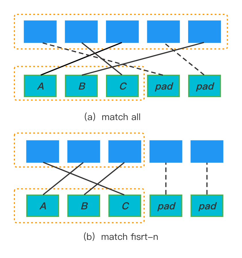
Figure 1: Two assignment schemes.

In practice, we design two assignment schemes for bipartite matching. The first scheme is to get the optimal matching between non-$\varnothing$ ground truth labels and all generated distributions, then assign $\varnothing$ labels to the rest generated distributions one-to-one. The second scheme is to get the optimal matching between non-$\varnothing$ ground truth labels and first-n generated distributions, then assign $\varnothing$ labels to the rest generated distributions one-to-one. Figure 1 shows the two assignment schemes.

Finally, we get the bipartite matching loss based on the reordered sequence $\boldsymbol{\hat{y}}=\{y_{\hat{\rho}(i)}\}_{i=1,\ldots,N}$ to train model, which is defined as follows:

$$\mathcal{L}_{b}(\boldsymbol{\hat{y}},\boldsymbol{p})=-\sum_{i=1}^{N}[\mathbbm{1}_{\{y_{\hat{\rho}(i)}\neq\varnothing\}}\log\boldsymbol{p}_{i}(y_{\hat{\rho}(i)})\\ +\mathbbm{1}_{\{y_{\hat{\rho}(i)}=\varnothing\}}\lambda_{\varnothing}\log\boldsymbol{p}_{i}(y_{\hat{\rho}(i)})]$$ (13)

where $\lambda_{\varnothing}$ is a scale factor less than $1$ that forces the model concentrate more on non-$\varnothing$ labels.

2.3.2 Semantic Optimal Transport Distance

In XMTC, semantic similar labels commonly appear together in each sample. The bipartite matching loss described in Eq.(13) only utilizes one value in each predictions. We completely utilize the predictions in training, and take the optimal transport (OT) distance in embedding space as a regularization term to make all predictions close to positive labels, as the shown in Figure 2.

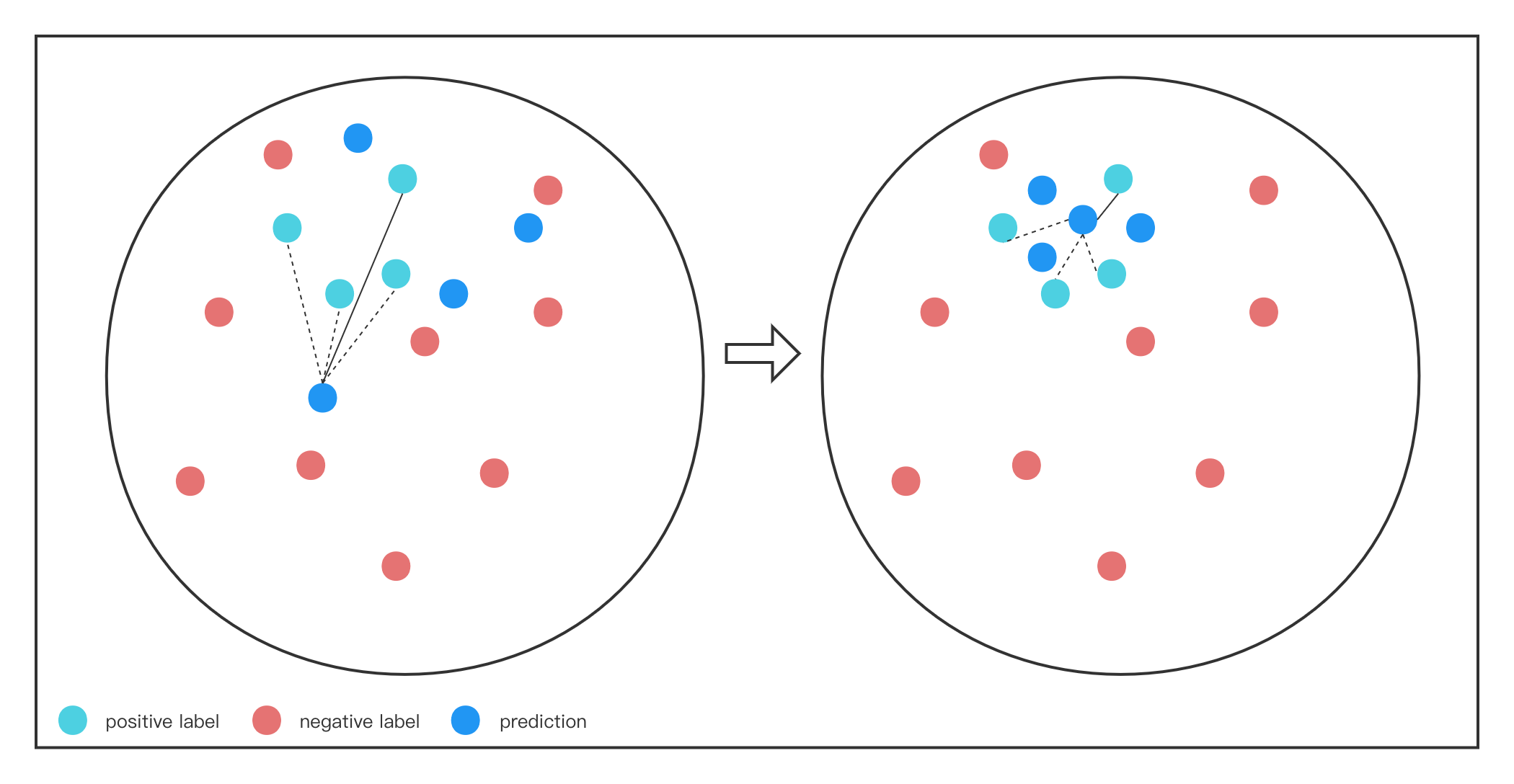
Figure 2: Semantic optimal transport distance in embedding space.

OT distance on discrete domain

The OT distance is also known as Wasserstein distance on a discrete domain $\mathbbm{X}$ (the sequence space), which is defined as follows:

$$\mathcal{L}_{ot}(\boldsymbol{p},\boldsymbol{y})=\min_{\boldsymbol{\Gamma}\in\Sigma(\boldsymbol{\mu},\boldsymbol{\nu})}\langle\boldsymbol{C},\boldsymbol{\Gamma}\rangle\\ =\min_{\boldsymbol{\Gamma}\in\Sigma(\boldsymbol{\mu},\boldsymbol{\nu})}\sum_{i=1}^{n}\sum_{j=1}^{m}\Gamma_{ij}\cdot c(\boldsymbol{p}_{i},y_{j}),$$ (14)

where $\boldsymbol{\mu}\in\mathbbm{R}_{+}^{n}$, $\boldsymbol{\nu}\in\mathbbm{{R}_{+}^{m}}$ are two discrete distributions on $\mathbbm{X}$, $\|\boldsymbol{\mu}\|=\|\boldsymbol{\nu}\|=1$. In our case, given realizations $\{\boldsymbol{p}_{i}\}_{i=1}^{n}$ and $\{y_{j}\}_{j=1}^{m}$ of $\boldsymbol{\mu}$ and $\boldsymbol{\nu}$, we can approximate them by empirical distributions $\boldsymbol{\widehat{\mu}}=\frac{1}{n}\sum_{\boldsymbol{p}_{i}}\delta_{\boldsymbol{p}_{i}}$ and $\boldsymbol{\widehat{\nu}}=\frac{1}{m}\sum_{y_{j}}\delta_{y_{j}}$. The supports of $\boldsymbol{\widehat{\mu}}$ and $\boldsymbol{\widehat{\nu}}$ are finite, so finally we have $\boldsymbol{\mu}=\frac{1}{n}\boldsymbol{1}_{\{\boldsymbol{p}_{i}\}}$ and $\boldsymbol{\nu}=\frac{1}{m}\boldsymbol{1}_{\{y_{j}\}}$. $\Sigma(\boldsymbol{\mu},\boldsymbol{\nu})$ is the set of joint distributions whose marginals are $\boldsymbol{\mu}$ and $\boldsymbol{\nu}$, which is described as $\Sigma(\boldsymbol{\mu},\boldsymbol{\nu})=\{\boldsymbol{\Gamma}\in\mathbbm{R}_{+}^{n\times m}|\boldsymbol{\Gamma}\boldsymbol{1}_{m}=\boldsymbol{\mu},\boldsymbol{\Gamma^{\top}}\boldsymbol{1}_{n}=\boldsymbol{\nu}\}$, where $\boldsymbol{1}_{n}$ represents n-dimensional vector of ones. Matrix $\boldsymbol{C}=[c(\boldsymbol{p}_{i},y_{j})]\in\mathbbm{R}_{+}^{n\times m}$ is the cost matrix, whose element $c(\boldsymbol{p}_{i},y_{j})$ denotes the distance between the $i$-th support point $\boldsymbol{p}_{i}\in\mathbbm{X}$ of $\boldsymbol{\mu}$ and the $j$-th support point $y_{j}\in\mathbbm{X}$ of $\boldsymbol{\nu}$. Notation $\langle\cdot,\cdot\rangle$ represents the Frobenius dot-product. With the optimal solution $\boldsymbol{\Gamma}^{*}$, $\mathcal{L}_{ot}(\boldsymbol{p},\boldsymbol{y})$ is the minimum cost that transport from distribution $\boldsymbol{\mu}$ to $\boldsymbol{\nu}$.

We use a robust and efficient iterative algorithm to compute the OT distance, which is the recently introduced Inexact Proximal point method for exact Optimal Transport (IPOT) (Xie et al., 2020).

Semantic Cost Function in OT

In XMTC learning, it’s intractable to directly compute the cost distance between predictions and ground-truth one-hot vector because of the huge label space. A more natural choice for computing cost distance is to use the label embeddings. Based on the rich semantics of embedding space, we can compute the semantic OT distance between model predictions and ground-truth. The details of computing the cosine distance are described as follows:

$$c(\boldsymbol{p}_{i},y_{j})=cosine\_distance(\boldsymbol{E}^{\top}\boldsymbol{p}_{i},\boldsymbol{E}^{\top}\mathbbm{1}_{y_{j}})$$ (15)

$$cosine\_distance(\boldsymbol{x},\boldsymbol{y})=1-\frac{\boldsymbol{x}^{\top}\boldsymbol{y}}{\|\boldsymbol{x}\|_{2}\|\boldsymbol{y}\|_{2}}$$ (16)

where $\boldsymbol{E}\in\mathbbm{R}^{V\times d}$ is the label embedding matrix, $V$ is the vocabulary size and $d$ is the dimension for the embedding vector. $\mathbbm{1}_{y_{j}}$ is the one-hot vector whose value is 0 in all positions except at position $y_{j}$ is 1.

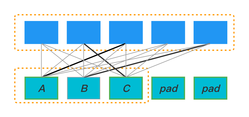
Figure 3: Semantic optimal transport distance.

In practice, we compute the semantic optimal transport distance $\mathcal{L}_{ot}(\boldsymbol{p},\boldsymbol{y})$ between non-$\varnothing$ ground-truth labels and all predictions, which is shown in 3.

2.3.3 Complete Seq2Set Training with OT regularization

The bipartite matching gives the optimal matching between ground truth and predictions, which enables the Seq2Set model to train with Maximum likelihood estimation (MLE). In addition, the OT distance provides a measurement in semantic label embedding space. We propose to combine the OT distance and the bipartite matching loss, which gives us the final training objective:

$$\mathcal{L}=\mathcal{L}_{b}(\boldsymbol{\hat{y}},\boldsymbol{p})+\lambda\mathcal{L}_{ot}(\boldsymbol{p},\boldsymbol{y})$$ (17)

where $\lambda$ is a hyper-parameter to be tuned.

Dataset	$N_{train}$	$N_{test}$	$D$	$L$	$\overline{L}$	$L_{max}$	$\hat{L}$	$\overline{W}_{train}$	$\overline{W}_{test}$
Eurlex-4K	15,449	3,865	186,104	3,956	5.30	24	20.79	1248.58	1230.40
Wiki10-31K	14,146	6,616	101,938	30,938	18.64	30	8.52	2484.30	2425.45
AmazonCat-13K	1,186,239	306,782	203,882	13,330	5.04	57	448.57	246.61	245.98
Amazon-670K	490,449	153,025	135,909	670,091	5.45	7	3.99	247.33	241.22

Table 1: Data Statistics. $N_{train}$ and $N_{test}$ refer to the number of training samples and test samples respectively. $D$ refers to the total number of features. $L$ is the total number of labels, $\overline{L}$ is the average number of labels per training sample, $L_{max}$ is the max length of labels for both training and test samples, $\hat{L}$ is the average number of samples per training label. $\overline{W}_{train}$ and $\overline{W}_{test}$ refer to the average number of words per training and test sample respectively.

3 Experiments

3.1 Datasets

We use four benchmark datasets, including three large-scale datasets Eurlex-4K (Loza Mencía and Fürnkranz, 2008) and AmazonCat-13K (McAuley and Leskovec, 2013) and Wiki10-31K (Zubiaga, 2012), one extreme-scale dataset Amazon-670K (McAuley and Leskovec, 2013). We follow the training and test split of AttentionXML (You et al., 2019) and we set aside 10% of the training instances as the validation set for hyperparameter tuning. The dataset statistics are summarized in Table 1.

3.2 Evaluation Metrics

Following the previous work (Yang et al., 2018, Nam et al., 2017, Yang et al., 2019), we evaluate all methods in terms of micro-F1 score, micro-precision and micro-recall are also reported for analysis.

3.3 Baselines

We compare our proposed methods with the following competitive baselines:

Seq2Seq (Bahdanau et al., 2015) is a classic Seq2Seq model with attention mechanism, which is also a strong baseline for XMTC tasks.

MLC2Seq (Nam et al., 2017) is based on Seq2Seq (Bahdanau et al., 2015), which enhances Seq2Seq model for MLC tasks by changing label permutations according to the frequency of labels. We take the descending order from frequent to rare in our experiments.

SGM (Yang et al., 2018) is based on previews Seq2Seq (Bahdanau et al., 2015) and MLC2Seq (Nam et al., 2017), which views the MLC task as a sequence generation problem to take the correlations between labels into account.

In order to extend the above three models to large-scale dataset Wiki10-31K and extreme-scale dataset Amazon-670K, we use the bottleneck layer to replace the fully connected layer. The bottleneck sizes are same as our proposed model and they are shown in Table 2.

3.4 Experiment Settings

For each dataset, the vocabulary size of input text is limited to 500,000 words according to the word frequency in the dataset.

The number of GRU layers of the encoder is 2, and for the decoder is 1. The hidden sizes of the encoder and the decoder both are 512. We set the max length of generated predictions $N$ to the max length of labels in each dataset are shown in Table 1 as $L_{max}$.

For LightConv, we set the kernel sizes to 3,7,15,30 for each layer respectively. To reduce the memory consumption of GPU, we set the stride of convolution to 3 in the last layer for all datasets except that Wiki10-31K is 4.

We set the hyperparameter $\lambda_{\varnothing}$ of bipartite matching loss to 0.2 in Eq.(13) following Ye et al. (2021), and $\lambda$ of final loss to 8 in Eq.(17).

For word embeddings in three baseline models and our proposed models, we use pre-trained 300-dimensional Glove vectors (Pennington et al., 2014) to all datasets for input text, and use the mean value of embeddings of words in labels for all datasets except for Amazon-670K, because the labels in Amazon-670K are corresponding item numbers and we randomly initialize 100-dimensional embeddings for Amazon-670K.

All models are trained by the Adam optimizer (Kingma and Ba, 2014) with a cosine annealing schedule. Besides, we use dropout (Srivastava et al., 2014) to avoid overfitting, the dropout rate is 0.2, and clip the gradients (Pascanu et al., 2013) to the maximum norm of 8.

All models are trained on one Nvidia TITAN V and one Nvidia GeForce RTX 3090, for the small dataset Eurlex-4K, we use TITAN V, and for others, we use RTX 3090.

Other hyperparameters are given in Table 2.

Datasets	$E$	$B$	$lr$	$b$	$L_{t}$
Eurlex-4K	20	32	0.001	-	1000
Wiki-31K	15	32	0.001	300	2000
AmazonCat-13K	5	64	0.0005	-	500
Amazon-670K	20	64	0.0005	512	500

Table 2: Hyperparameters of all datasets. $E$ is the number of epochs, $B$ is the batch size, $lr$ is init learning rate, $b$ is the bottleneck size (Note that the bottleneck layer is not used on Eurlex-4K and AmanzonCat-13K), $L_{t}$ is the maximum length of input tokens.

Methods	P	R	F1
Eurlex-4K
Seq2Seq	60.83	54.76	57.64
MLC2Seq	59.80	56.70	58.21
SGM	59.99	56.56	58.23
Seq2Seq + LC	61.36	55.03	58.02
$\mathrm{BM}_{all}$	61.72	57.63	59.61
$\mathrm{BM}_{all}$ + LC	63.38	58.10	60.63
$\mathrm{BM}_{all}$ + OT	65.95	58.54	62.03
$\mathrm{BM}_{all}$ + OT + LC	64.82	60.26	62.46

Methods	P	R	F1
Wiki10-31K
Seq2Seq	29.87	26.96	28.34
MLC2Seq	28.69	28.03	28.36
SGM	28.89	27.93	28.40
Seq2Seq + LC	30.06	27.14	28.53
$\mathrm{BM}_{first-n}$	33.23	29.43	31.22
$\mathrm{BM}_{first-n}$ + LC	33.58	29.94	31.66
$\mathrm{BM}_{first-n}$ + OT	37.26	29.08	32.67
$\mathrm{BM}_{first-n}$ + OT + LC	36.70	30.05	33.04

Amazon-670K
Seq2Seq	32.16	32.04	32.10
MLC2Seq	30.27	32.32	31.26
SGM	30.12	31.42	30.76
Seq2Seq + LC	31.15	31.32	31.24
$\mathrm{BM}_{all}$	55.23	27.33	36.56
$\mathrm{BM}_{all}$ + LC	52.70	26.30	35.09
$\mathrm{BM}_{all}$ + OT	58.36	26.46	36.42
$\mathrm{BM}_{all}$ + OT + LC	61.16	26.39	36.87

AmazonCat-13K
Seq2Seq	74.26	68.24	71.12
MLC2Seq	70.93	69.66	70.29
SGM	71.27	69.36	70.30
Seq2Seq + LC	74.60	68.49	71.41
$\mathrm{BM}_{first-n}$	70.26	72.51	71.37
$\mathrm{BM}_{first-n}$ + LC	70.46	72.95	71.68
$\mathrm{BM}_{first-n}$ + OT	71.80	71.57	71.69
$\mathrm{BM}_{first-n}$ + OT + LC	71.98	71.71	71.84

Table 3: Comparison between our models and three baselines on Eurlex-4K, Wiki10-31K, Amazon-670K, and AmazonCat-13K. $\mathrm{BM}_{all}$ denotes the Seq2Seq model with the first scheme of bipartite matching loss, $\mathrm{BM}_{first-n}$ denotes the Seq2Seq model with the second one. OT denotes the semantic optimal transport distance loss. LC denotes the light weight convolution layer. We take the average score of 4 times experiments for all models on Eurlex-4K and Wiki10-31K, and 2 times experiments for the other two datasets.

3.5 Main Results

Table 3 compares the proposed methods with three baselines on four benchmark datasets. We focus on micro-F1 score following previous works based on Seq2Seq. The best score of each metric is in boldface. Our models outperform all baselines in micro-F1 score. We find that the two assignment scheme of bipartite matching each excel on different datasets. $\mathrm{BM}_{all}$ denotes the Seq2Seq model with the first scheme of bipartite matching, $\mathrm{BM}_{first-n}$ denotes the Seq2Seq model with the second one. $\mathrm{BM}_{all}$ has the better performance on Eurlex-4K and Amazon-670K, rather $\mathrm{BM}_{first-n}$ is better on Wiki10-31K and AmazonCat-13K. Our complete method achieves a large improvement of 16.34% micro-F1 score over the second best baseline model which is SGM on Wiki10-31K, and 14.86%, 7.26%, 1.01% on other datasets respectively, the relative impovements are shown in Table 4.

Methods	Eurlex-4K	Wiki10-31K	Amazon-670K	AmazonCat-13K
$\mathrm{BM}$	2.37%	9.93%	13.89%	0.35%
$\mathrm{BM}$ + OT	6.53%	15.04%	13.46%	0.8%
$\mathrm{BM}$ + OT + LC	7.26%	16.34%	14.86%	1.01%

Table 4: Relative improvements of micro-F1 score over the second best baseline model on four datasets in Table 3. $\mathrm{BM}$ denotes $\mathrm{BM}_{all}$ or $\mathrm{BM}_{first-n}$.

3.6 $\boldsymbol{\mathrm{BM}_{first-n}}$ vs $\boldsymbol{\mathrm{BM}_{all}}$

We find that the different performance of $\mathrm{BM}_{first-n}$ and $\mathrm{BM}_{all}$ are related to the distribution of label size on the dataset. Table 5 compares $\mathrm{BM}_{first-n}$ with $\mathrm{BM}_{all}$ in micro-F1 score on all datasets. The performance difference on Eurlex-4K is very small since the two proportions which are shown in Figure 4 are nearly equal. Wiki10-31K is the same case. However, the two proportions have a big difference on AmanzonCat-13K and Amazon-670K, which leads to the large performance difference between $\mathrm{BM}_{first-n}$ and $\mathrm{BM}_{all}$. The proportion of samples whose label size is smaller than the average is less than 50%, then the performance of $\mathrm{BM}_{first-n}$ is better than $\mathrm{BM}_{all}$. The proportion of samples whose label size is greater than average number is greater than 50%, then the performance of $\mathrm{BM}_{all}$ is better than $\mathrm{BM}_{first-n}$.

Datasets	$\mathrm{BM}_{all}$	$\mathrm{BM}_{first-n}$
Eurlex-4K	59.61	59.12($\downarrow 0.82\%$)
Wiki10-31K	31.38	31.22($\downarrow 0.51\%$)
AmazonCat-13K	67.09	71.37($\uparrow 6.38\%$)
Amazon-670K	36.87	34.45($\downarrow 6.56\%$)

Table 5: The micro-F1 score of $\mathrm{BM}_{all}$ and $\mathrm{BM}_{first-n}$ and relative difference on four datasets.

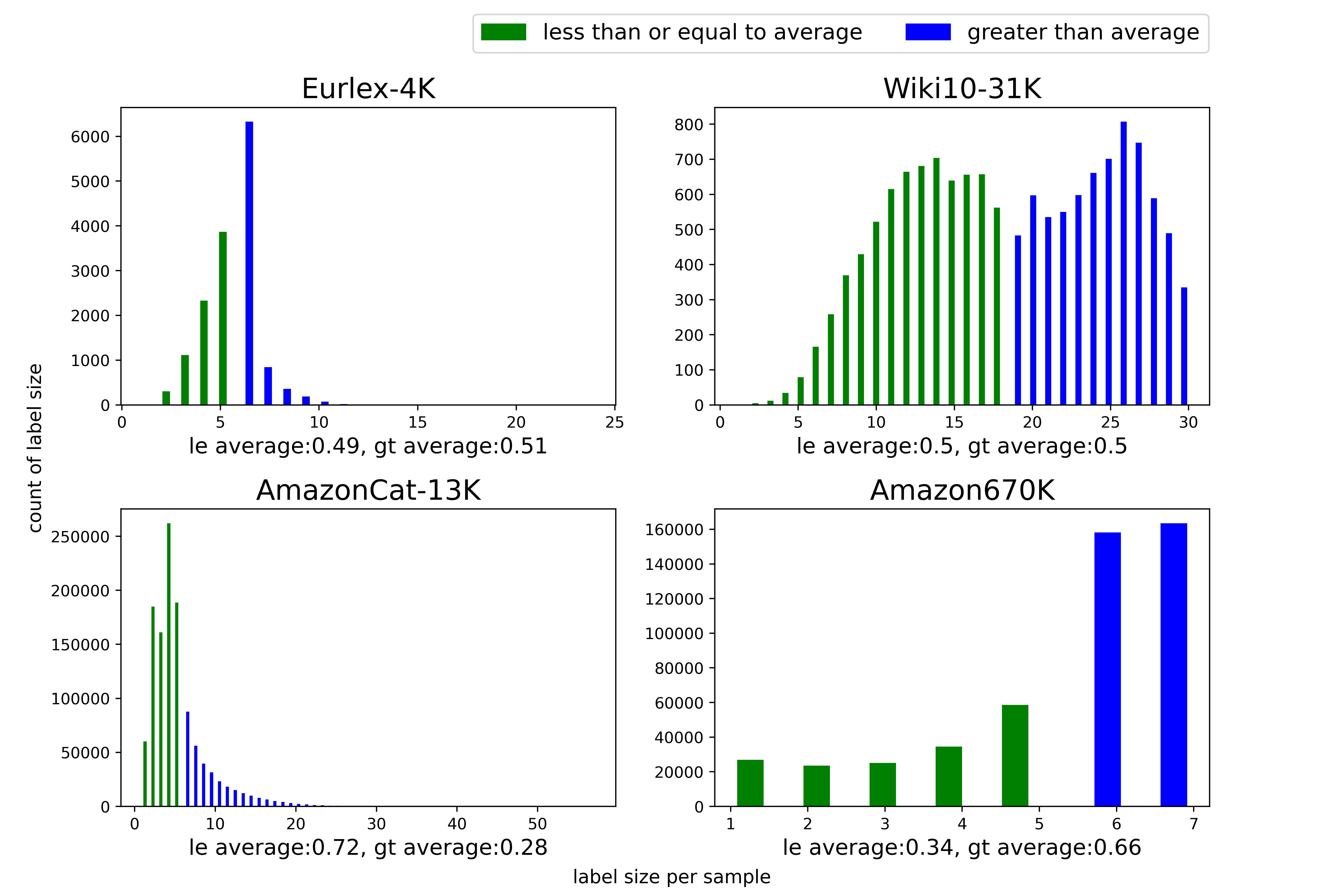
Figure 4: Distributions of label size on all datasets. The le average denotes the proportion of samples whose label size less than or equal to average number of label size, the gt average denotes the opposite proportion.

3.7 Effect of Lightweight Convolution and Semantic Optimal Transport Distance

To examine the effect of LightConv and OT, we add LightConv to the Seq2seq model and $\mathrm{BM}$ model, and add OT to $\mathrm{BM}$ model. The details of results are shown in Table 3. The semantic optimal transport distance and LigntConv achieve improvements against origin models on all datasets except for Amazon-670K, but it’s not beyond our imagination, because Amazon-670K has an extremely large label set which is item numbers. The item numbers don’t have semantic information leading to OT having no effect. At the same time Amazon-670K has the lowest average number of samples per label, it’s very hard to learn a proper context vector by the LightConv. However, the combination of OT and LightConv still has a small improvement over $\mathrm{BM}_{all}$ methods on Amazon-670K.

3.8 Comprehensive Comparison

To realize the performance of our method on tail labels, we use the macro-averaged F1 (maF1) score which treats all labels equally regardless of their support values. To more comprehensively compare our model with baselines, we also use the weighted-averaged F1 (weF1) which considers each label’s support, and the example-based F1 (ebF1) which calculates F1 score for each instance and finds their average. We show the results in Table 6.

Methods	maF1	weF1	ebF1
Eurlex-4K
Seq2Seq	23.26	55.36	57.10
MLC2Seq	24.16	56.24	58.00
SGM	24.32	56.28	57.96
$\mathrm{OTSeq2Set}_{all}$	27.34	60.45	61.04

Methods	maF1	weF1	ebF1
Wiki10-31K
Seq2Seq	3.51	24.55	27.97
MLC2Seq	4.85	26.15	28.14
SGM	4.29	26.00	28.19
$\mathrm{OTSeq2Set}_{first-n}$	3.50	26.55	32.65

Amazon-670K
Seq2Seq	11.57	30.29	29.62
MLC2Seq	11.55	30.36	29.62
SGM	11.14	29.53	28.85
$\mathrm{OTSeq2Set}_{all}$	9.91	28.83	25.65

AmazonCat-13K
Seq2Seq	41.28	69.37	74.03
MLC2Seq	39.79	68.78	73.57
SGM	40.44	68.96	73.68
$\mathrm{OTSeq2Set}_{first-n}$	43.42	70.95	75.18

Table 6: Performance comparison of all models on the macro-averaged F1, the weighted- averaged F1 and the example-based F1.

3.9 Performance over different $\lambda$

We conduct experiments on Eurlex4K dataset to evaluate performance with different hyperparameter $\lambda$ in complete loss function $\mathcal{L}$. The results are shown in Figure 5. The figure shows that when $\lambda=8$, the performance reaches its best and is stable.

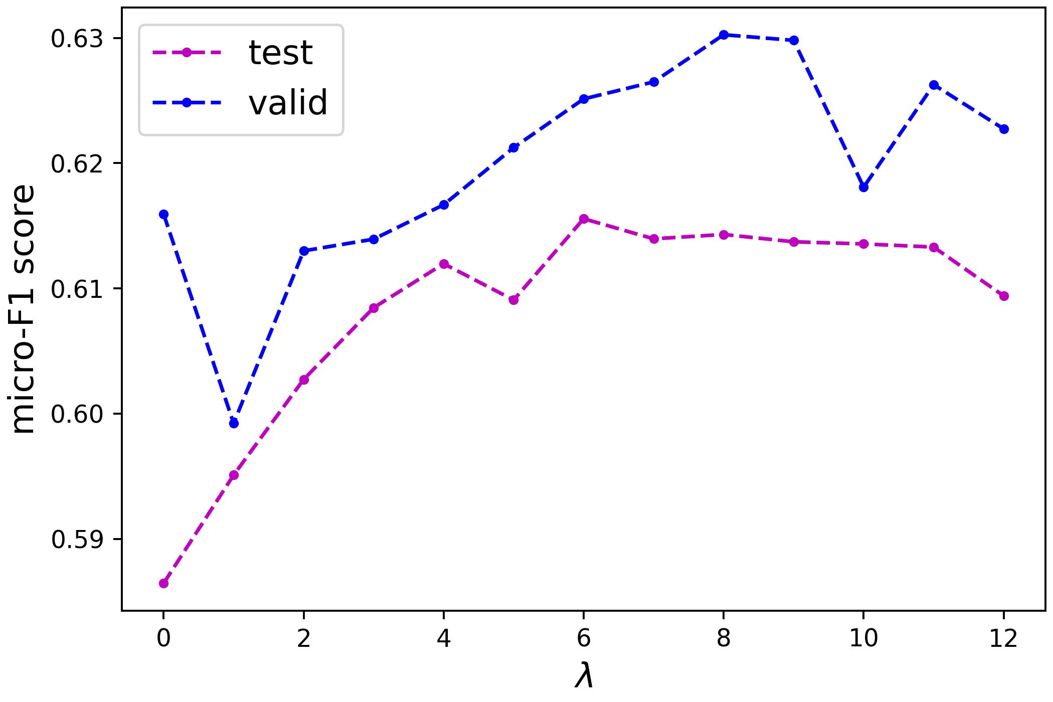
Figure 5: Performance of the OTSeq2Set using different $\lambda$ in loss function.

3.10 Computation Time and Model Size

Table 7 shows the overall training time of all models compared in our experiments. The MLC2Seq has the same model size and training time as Seq2Seq. The model size of OTSeq2Set is almost the same as that of Seq2Seq, but the overall training time is much longer than other models, because the bipartite matching loss and the optimal transport distance need to compute for each sample individually.

Datasets		Seq2Seq	SGM	OTSeq2Set
Eurlex-4K	$T_{train}$	0.85	0.85	1.52
	$M$	34.8	35.0	40.5
Wiki10-31K	$T_{train}$	1.55	1.56	1.78
	$M$	45.5	45.7	47.5
AmazonCat-13K	$T_{train}$	3.70	3.75	17.88
	$M$	54.8	55.0	70.1
Amazon-670K	$T_{train}$	12.9	16.0	18.5
	$M$	437.7	437.7	439.8

Table 7: Training Time and Model Size. $T_{train}$ is the overall training hours. $M$ is the total size of model parameters in millions.

4 Related Work

The most popular deep learning models in XMTC are fully connected layer based models. XML-CNN (Liu et al., 2017) uses a convolutional neural network (CNN) and a dynamic max pooling scheme to learn the text representation, and adds an hidden bottleneck layer to reduce model size as well as boost model performance. AttentionXML (You et al., 2019) utilizes a probabilistic label tree (PLT) to handle millions of labels. In AttentionXML, a BiLSTM is used to capture long-distane dependency among words and a multi-label attention is used to capture the most relevant parts of texts to each label. CorNet (Xun et al., 2020) proposes a correlation network (CorNet) capable of ulilizing label correlations. X-Transformers (Chang et al., 2020) proposes a scalable approach to fine-tuning deep transformer models for XMTC tasks, which is also the first method using deep transformer models in XMTC. LightXML (Jiang et al., 2021) combines the transformer model with generative cooperative networks to fine-tune transformer model.

Another type of deep learning-based method is Seq2Seq learning based methods. MLC2Seq (Nam et al., 2017) is based on the classic Seq2Seq (Bahdanau et al., 2015) architecture which uses a bidirectional RNN to encode raw text and an RNN with an attention mechanism to generate predictions sequentially. MLC2Seq enhances the model performance by determining label permutations before training. SGM (Yang et al., 2018) proposes a novel decoder structure to capture the correlations between labels. Yang et al. (2019) proposes a two-stage training method, which is trained with MLE then is trained with a self-critical policy gradient training algorithm.

About bipartite matching, Tan et al. (2021) considers named entity recognition as a Seq2Set task, the model generates an entity set by a non-autoregressive decoder and is trained by a loss function based on bipartite matching. ONE2SET (Ye et al., 2021) proposes a K-step target assignment mechanism via bipartite matching on the task of keyphrases generation, which also uses a non-autoregressive decoder.

Xie et al. (2020) proposes a fast proximal point method to compute the optimal transport distance, which is named as IPOT. Chen et al. (2019) adds the OT distance as a regularization term to the MLE training loss. The OT distance aims to find an optimal matching of similar words/phrases between two sequences which promotes their semantic similarity. Li et al. (2020) introduce a method that combines the student-forcing scheme with the OT distance in text generation tasks, this method can alleviate the exposure bias in Seq2Seq learning. The above two methods both use the IPOT to compute the OT distance.

5 Conclusion

In this paper, we propose an autoregressive Seq2Set model for XMTC, OTSeq2Set, which combines the bipartite matching and the optimal transport distance to compute overall training loss and uses the student-forcing scheme in the training state. OTSeq2Set not only eliminates the influence of order in labels, but also avoids the exposure bias. Besides, we design two schemes for the bipartite matching which are suitable for datasets with different label distributions. The semantic optimal transport distance can enhance the performance by the semantic similarity of labels. To take full advantage of the raw text information, we add a lightweight convolution module which achieves a stable improvement and requires only a few parameters. Experiments show that our method gains significant performance improvements against strong baselines on XMTC.

Limitations

For better effect, we compute the bipartite matching and the optimal transport distance between non-$\varnothing$ targets and predictions. We can’t use batch computation to improve efficiency so that the training time of OTSeq2Set is longer than other baseline models.

References

- Bahdanau et al. (2015) Dzmitry Bahdanau, Kyunghyun Cho, and Yoshua Bengio. 2015. Neural machine translation by jointly learning to align and translate. CoRR, abs/1409.0473.
- Chang et al. (2020) Wei-Cheng Chang, Hsiang-Fu Yu, Kai Zhong, Yiming Yang, and Inderjit S. Dhillon. 2020. Taming pretrained transformers for extreme multi-label text classification. In Proceedings of the 26th ACM SIGKDD International Conference on Knowledge Discovery & Data Mining, KDD ’20, page 3163–3171, New York, NY, USA. Association for Computing Machinery.
- Chen et al. (2019) Liqun Chen, Yizhe Zhang, Ruiyi Zhang, Chenyang Tao, Zhe Gan, Haichao Zhang, Bai Li, Dinghan Shen, Changyou Chen, and Lawrence Carin. 2019. Improving sequence-to-sequence learning via optimal transport. In International Conference on Learning Representations.
- Jiang et al. (2021) Ting Jiang, Deqing Wang, Leilei Sun, Huayi Yang, Zhengyang Zhao, and Fuzhen Zhuang. 2021. Lightxml: Transformer with dynamic negative sampling for high-performance extreme multi-label text classification. In AAAI.
- Kingma and Ba (2014) Diederik P Kingma and Jimmy Ba. 2014. Adam: A method for stochastic optimization. arXiv preprint arXiv:1412.6980.
- Kuhn (1955) Harold W Kuhn. 1955. The hungarian method for the assignment problem. Naval research logistics quarterly, 2(1-2):83–97.
- Li et al. (2020) Jianqiao Li, Chunyuan Li, Guoyin Wang, Hao Fu, Yuhchen Lin, Liqun Chen, Yizhe Zhang, Chenyang Tao, Ruiyi Zhang, Wenlin Wang, Dinghan Shen, Qian Yang, and Lawrence Carin. 2020. Improving text generation with student-forcing optimal transport. In Proceedings of the 2020 Conference on Empirical Methods in Natural Language Processing (EMNLP), pages 9144–9156. Association for Computational Linguistics.
- Liu et al. (2017) Jingzhou Liu, Wei-Cheng Chang, Yuexin Wu, and Yiming Yang. 2017. Deep learning for extreme multi-label text classification. In Proceedings of the 40th International ACM SIGIR Conference on Research and Development in Information Retrieval, pages 115–124. ACM.
- Loza Mencía and Fürnkranz (2008) Eneldo Loza Mencía and Johannes Fürnkranz. 2008. Efficient pairwise multilabel classification for large-scale problems in the legal domain. In Machine Learning and Knowledge Discovery in Databases, pages 50–65. Springer Berlin Heidelberg.
- McAuley and Leskovec (2013) Julian McAuley and Jure Leskovec. 2013. Hidden factors and hidden topics: understanding rating dimensions with review text. In Proceedings of the 7th ACM conference on Recommender systems, pages 165–172. ACM.
- Nam et al. (2017) Jinseok Nam, Eneldo Loza Mencía, Hyunwoo J Kim, and Johannes Fürnkranz. 2017. Maximizing subset accuracy with recurrent neural networks in multi-label classification. In Advances in Neural Information Processing Systems, volume 30. Curran Associates, Inc.
- Pascanu et al. (2013) Razvan Pascanu, Tomas Mikolov, and Yoshua Bengio. 2013. On the difficulty of training recurrent neural networks. In International conference on machine learning, pages 1310–1318. PMLR.
- Pennington et al. (2014) Jeffrey Pennington, Richard Socher, and Christopher Manning. 2014. Glove: Global vectors for word representation. In Proceedings of the 2014 Conference on Empirical Methods in Natural Language Processing (EMNLP), pages 1532–1543. Association for Computational Linguistics.
- Ranzato et al. (2016) Marc’Aurelio Ranzato, Sumit Chopra, Michael Auli, and Wojciech Zaremba. 2016. Sequence level training with recurrent neural networks. CoRR, abs/1511.06732.
- Srivastava et al. (2014) Nitish Srivastava, Geoffrey Hinton, Alex Krizhevsky, Ilya Sutskever, and Ruslan Salakhutdinov. 2014. Dropout: a simple way to prevent neural networks from overfitting. The journal of machine learning research, 15(1):1929–1958.
- Tan et al. (2021) Zeqi Tan, Yongliang Shen, Shuai Zhang, Weiming Lu, and Yueting Zhuang. 2021. A sequence-to-set network for nested named entity recognition. In Proceedings of the Thirtieth International Joint Conference on Artificial Intelligence, pages 3936–3942. International Joint Conferences on Artificial Intelligence Organization.
- Wu et al. (2019) Felix Wu, Angela Fan, Alexei Baevski, Yann Dauphin, and Michael Auli. 2019. Pay less attention with lightweight and dynamic convolutions. In International Conference on Learning Representations.
- Xie et al. (2020) Yujia Xie, Xiangfeng Wang, Ruijia Wang, and Hongyuan Zha. 2020. A fast proximal point method for computing exact wasserstein distance. In Uncertainty in artificial intelligence, pages 433–453. PMLR.
- Xun et al. (2020) Guangxu Xun, Kishlay Jha, Jianhui Sun, and Aidong Zhang. 2020. Correlation networks for extreme multi-label text classification. In Proceedings of the 26th ACM SIGKDD International Conference on Knowledge Discovery & Data Mining, pages 1074–1082. ACM.
- Yang et al. (2019) Pengcheng Yang, Fuli Luo, Shuming Ma, Junyang Lin, and Xu Sun. 2019. A deep reinforced sequence-to-set model for multi-label classification. In Proceedings of the 57th Annual Meeting of the Association for Computational Linguistics, pages 5252–5258. Association for Computational Linguistics.
- Yang et al. (2018) Pengcheng Yang, Xu Sun, Wei Li, Shuming Ma, Wei Wu, and Houfeng Wang. 2018. SGM: Sequence generation model for multi-label classification. In Proceedings of the 27th International Conference on Computational Linguistics, pages 3915–3926. Association for Computational Linguistics.
- Ye et al. (2021) Jiacheng Ye, Tao Gui, Yichao Luo, Yige Xu, and Qi Zhang. 2021. One2set: Generating diverse keyphrases as a set. In Proceedings of the 59th Annual Meeting of the Association for Computational Linguistics and the 11th International Joint Conference on Natural Language Processing (Volume 1: Long Papers), pages 4598–4608. Association for Computational Linguistics.
- You et al. (2019) Ronghui You, Zihan Zhang, Ziye Wang, Suyang Dai, Hiroshi Mamitsuka, and Shanfeng Zhu. 2019. Attentionxml: Label tree-based attention-aware deep model for high-performance extreme multi-label text classification. In NeurIPS.
- Zubiaga (2012) Arkaitz Zubiaga. 2012. Enhancing navigation on wikipedia with social tags. Number: arXiv:1202.5469.