Universal robust quantum gates by geometric correspondence of noisy quantum dynamics

Abstract

Exposure to noises is a major obstacle for processing quantum information, but noises don’t necessarily induce errors. Errors on the quantum gates could be suppressed via robust quantum control techniques. But understanding the genesis of errors and finding a universal treatment remains grueling. To resolve this issue, we develop a geometric theory to graphically capture quantum dynamics due to various noises, obtaining the quantum erroneous evolution diagrams (QEED). Our theory provides explicit necessary and sufficient criteria for robust control Hamiltonian and quantitative geometric metrics of the gate error. We then develop a protocol to engineer a universal set of single- and two-qubit robust gates that correct the generic errors. Our numerical simulation shows gate fidelities above $99.99\%$ over a broad region of noise strength using simplest and smooth pulses for arbitrary gate time. Our approach offers new insights into the geometric aspects of noisy quantum dynamics and several advantages over existing methods, including the treatment of arbitrary noises, independence of system parameters, scalability, and being friendly to experiments.

I Introduction

Paving the way to the future of quantum technologies and quantum computing hinges upon our ability to exercise precise and robust control over inherently noisy quantum systems. [1, 2, 3, 4, 5, 6, 7, 8]. Recent progress has pushed the quality of quantum gates to approach the fault-tolerant threshold in isolated characterizations [9, 10, 11, 12]; Yet, realistic multi-qubit systems are subject to a myriad of noises coupling to all system operators, precipitating quantum decoherence and gate errors [13, 14]. Remarkably, these noises do not invariably breed errors in quantum operations driven by evolution under specific control fields. Robust quantum gates, critical in integrating a large array of qubits [15, 16, 17, 18, 19], have been fashioned to dynamically correct errors [20, 21, 22, 23]. Conventionally, these gates are synthesized through pulse-shaping techniques that exploit numerical optimization, a method increasingly constrained by computational cost [24, 25, 26, 27, 28, 29], and potentially inapplicable to arbitrary noise models or scalable multi-qubit systems. Alternatives employ the geometric phase accrued via cyclic quantum evolution, achieving immunity to specific noise types but at the cost of slower gates [30, 31, 32, 33, 34]. To better engineer the control field at pulse-level, perturbative treatment of various noises has been utilized to study noisy quantum dynamics [35], leading to the proposal of dynamically-corrected gates designed to manage dephasing noises by mapping evolution onto geometric curves [21, 22, 23]. Nonetheless, both geometric methods grapple with significant challenges and practical constraints, including the limitation to a single error in a single qubit [21]. Realistic systems are subject to various noises that couple to all system operators. They may arise from inaccurate chip characterization, disturbances during quantum control, scalability issues due to excessive control lines, unwanted interactions, and crosstalk, etc [36]. Thus, a robust quantum gate’s resilience to such noise combinations becomes crucial. Therefore, our focus must be on comprehending the genesis of errors in noisy quantum dynamics and the control field’s error correction mechanisms within this noise-laden backdrop.

In this manuscript, we establish the essential correspondence between the noisy quantum dynamics and multiplex space curves that form a diagram to analyze control errors, which we call the quantum erroneous evolution diagrams (QEED). These curves are parametrized by generalized Frenet-Serret frames and thus enable a bijective map with the Hamiltonian. We use the multiplex curve diagrams to characterize the noisy quantum evolution quantitatively. We show that the diagrams provide quantitative metrics of the control robustness to different noises. We derive the necessary and sufficient conditions for general robust control. To make this theoretical framework applicable for robust control in experiments, we develop a simple and systematic protocol to find arbitrary robust control pulses with the simplest waveforms, consisting of only a few Fourier components. This protocol could be automated given only the system parameters, making it convenient for experiments. We demonstrate that these pulses could have arbitrary gate time while preserving the same robustness. We use these pulses to implement universal robust quantum gates. For the first time, we use realistic multi-qubit models of semiconductor quantum dots and superconducting transmons for numerical simulations. We obtain high gate-fidelity plateaus above the fault-tolerant threshold over a wide range of noise strength. These results demonstrate the effectiveness of our framework and suggest its potential applications. Our work provides a new perspective on noisy quantum dynamics and their relation to robust control by revealing an essential geometric correspondence between them. Our work also offers a practical solution for engineering universal robust quantum gates with simple pulses that are ready for experiments.

The paper is organized as follows: In Sec.IIII, we present our analytical theory based on QEED; in Sec.IIIIII we develop our protocol for finding robust control pulses; in Sec.IVIV, we apply our protocol to realistic models of spin qubits and transmons and present the outstanding results of robust gates; in Sec.VV, we discuss some extensions and limitations of our approach and then conclude with some remarks. Some details about the derivation and numerical results are presented in the Supplemental Materials.

II Analytical theory

II.1 Model settings

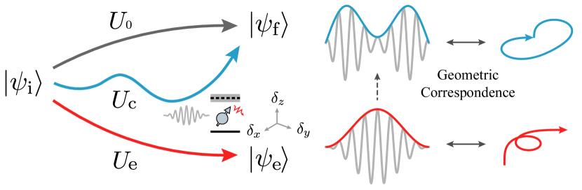
Figure 1: The illustration of geometric correspondence between noisy quantum dynamics and QEED. The black trajectory corresponds to the ideal unitary evolution $U_{0}$ that drives an initial quantum state to a desired final state. Realistic systems subject to errors in the longitudinal direction, $\delta_{z}$, and transverse direction, $\delta_{x}$ and $\delta_{y}$ undergo the colored trajectories with different control fields. The blue and red evolution trajectories are respectively driven by the robust pulse (blue) and cosine pulse (red) in the middle, corresponding to the blue and red geometric curves on the right.

We start from the generic Hamiltonian with a control field

$$H(t)=H_{0}+H_{c}(t)+V.$$ (1)

Here the system Hamiltonian $H_{0}$ added with the control term $H_{c}(t)$ generates the desired time evolution. $V=\bm{\delta}\cdot\hat{\mathbf{O}}$ is the noise term, where vector $\bm{\delta}$’s components are random complex numbers corresponding to quantum and classical noises [37, 38] that couple to the target quantum system via the operators $\hat{\mathbf{O}}=\{O_{1},...,O_{n}\}$. In the SU(2) subspace, $\hat{\mathbf{O}}=\hat{\bm{\sigma}}$ and $\hat{\bm{\sigma}}$ is the vector of Pauli operators. $\bm{\delta}$ is generally time-dependent and randomly fluctuating, which could be caused by unwanted effects including uncontrollable frequency shifts, spectrum broadening, crosstalk, parameter fluctuations, residual couplings [14, 39], etc.

The idea of robust control using the geometric correspondence is illustrated in Fig. 1. A trivial control field $H_{c}(t)$, for example, a cosine pulse, supposedly drives the raw system $H_{0}$ to a target final state $|\psi_{f}\rangle$. But subject to the noise $V$, the system’s evolution deviates from the ideal trajectory $U_{0}$ and undergoes a noisy evolution $U_{e}$. The erroneous final state $|\psi_{e}\rangle$ has an unknown distance from the desired final state depending on the noise strength. To correct the errors, control Hamiltonian $H_{c}(t)$ formed with robust control pulse (RCP) obtained by geometric correspondence should drive the system to the expected state $|\psi_{f}\rangle$, disregarding the presence of the unknown errors. This means that at some time $\tau$, $U_{c}(\tau)=U_{0}$. Nonetheless, solving the RCP is very challenging. We will show how to formulate error measures of control pulses and construct arbitrary RCPs, by establishing the geometric correspondence between space curves and the noisy quantum dynamics.

In order to obtain analytical solutions, our theory is formulated on the two-state systems, giving the SU(2) dynamics. The dynamics of higher dimensional systems correspond to more complex geometric structures and are beyond the scope of this manuscript. However, some complex system’s dynamics could be decomposed into direct sums or products of SU(2) operators, then the work presented in this manuscript still applies. The raw Hamiltonian for a single two-state Hilbert space $\text{span}\{\left|a\right\rangle,\left|b\right\rangle\}$ is $H_{raw}=-\frac{\omega}{2}\sigma_{z}$. If driven transversely with a control field, it is usually written in the rotating frame with the control field

$$H_{0}^{rot}=-\frac{\Delta}{2}\sigma_{z},$$ (2)

where $\Delta$ is the detuning between qubit frequency and control field. The formulas in this manuscript are all present in the rotating frame, so in the following, we will drop the superscript "rot". The control and the noise Hamiltonian could be written in the general form

$$H_{c}(t) = \Omega_{z}(t)\sigma_{z}+\Omega_{x}(t)\sigma_{x}+\Omega_{y}(t)\sigma_{y}$$ (3)

$$V = \delta_{z}\sigma_{z}+\delta_{x}\sigma_{x}+\delta_{y}\sigma_{y},$$ (4)

where the Pauli matrices $\sigma_{x}=|a\rangle\langle b|+|b\rangle\langle a|$, $\sigma_{y}=-i|a\rangle\langle b|+i|b\rangle\langle a|$, $\sigma_{z}=|a\rangle\langle a|-|b\rangle\langle b|$.

The error $\delta_{z}$ is related to many types of longitudinal noises including variations in frequency or fluctuating spectral splitting, which could originate from the coupling to other quantum systems, e.g., the neighboring qubits, two-level defects, or quantum bath [40, 41]. On the other hand, the transverse errors $\delta_{x}$ and $\delta_{y}$ result from energy exchange with the environment, such as relaxation, crosstalk, and imperfect control. In this manuscript, the formulation of the theory assumes that the noise fluctuation time scale is longer than a quantum gate. So $\bm{\delta}$ is a constant vector in this quasi-static limit.

Based on this assumption, we will show how to engineer the control Hamiltonian to correct the errors in its perpendicular directions. And hence for generic errors in the $x,y,z$ directions we need controls in at least directions, i.e., two terms out of the three in control Hamiltonian in Eq. (3) are sufficient to achieve dynamical error suppression. Specifically in the following discussion, we let

$$H_{c}(t)=\frac{\Omega(t)\cos\Phi(t)}{2}\sigma_{x}+\frac{\Omega(t)\sin\Phi(t)}{2}\sigma_{y},$$ (5)

where $\Omega(t)$ and $\Phi(t)$ are the control amplitude and modulated phase of the transverse control field.

II.2 Geometric correspondence

Here we present the essential geometric correspondence between the driven noisy quantum dynamics and space curves, based on which we further establish the robust control constraints. Given that the total time evolution reads $U(t)=\mathcal{T}\exp\{-i\int_{0}^{t}H(\tau)d\tau\}$, generated by the full noisy Hamiltonian $H(t)$ given in Eq. (1), whereas the noiseless driven dynamics evolves as $U_{0}(t)=\mathcal{T}\exp\{-i\int_{0}^{t}(H_{0}+H_{c}(\tau))d\tau\}$. In the interaction picture with $U_{0}(t)$, the total Hamiltonian is transformed to $V_{I}=U_{0}^{\dagger}VU_{0}=U_{0}^{\dagger}(\bm{\delta}\cdot\hat{\bm{\sigma}})U_{0}$. Our model settings have assumed time-independent errors, so $\bm{\delta}$ is a constant for time-integral. For the $j$-component of the noise source, the transformation $U_{0}^{\dagger}(t)\sigma_{j}U_{0}(t)$ over duration $dt$ gives rise to a displacement of the operator $d\bm{r}^{j}(t)\cdot\hat{\bm{\sigma}}$, while its time derivative defines a velocity $\bm{T}_{j}(t)=\dot{\bm{r}}^{j}(t)$. As $||\bm{T}_{j}||=||U_{0}^{\dagger}(t)\sigma_{j}U_{0}(t)||=1$, $\bm{T}_{j}$ is a unit vector which means the $j$-error motion has a constant speed. So the Hamiltonian has the geometric correspondence

$$V_{I}(t) =\delta_{x}\mathbf{T}_{x}(t)\cdot\hat{\bm{\sigma}}+\delta_{y}\mathbf{T}_{y}(t)\mathbf{\cdot}\hat{\bm{\sigma}}+\delta_{z}\mathbf{T}_{z}(t)\cdot\hat{\bm{\sigma}}$$

$$=\sum_{j,k=x,y,z}\delta_{j}T_{jk}(t)\sigma_{k}.$$ (6)

Here $T_{jk}(t)$ is a tensor connecting $j$-component of the noise source $\delta_{j}$ and Pauli term $\sigma_{k}$.

Because $U(t)=U_{0}(t)U_{I}(t)$, $U_{I}(t)$ could be called the erroneous evolution referring to the deviation of the noisy $U(t)$ from the noiseless $U_{0}(t)$. $U_{I}(t)$ is generated by the Hamiltonian in the interaction picture following the integral in time order as

$$U_{I}(t) =\mathcal{T}\exp\{-i\int_{0}^{t}d\tau V_{I}(t)\}$$

$$=\mathcal{T}\exp\{-i\sum_{j=x,y,z}\delta_{j}\int_{0}^{t}d\tau[\mathbf{T}_{j}(t)\cdot\hat{\bm{\sigma}}\mathbf{]}\}$$

$$=\mathcal{T}\exp\{-i\sum_{j=x,y,z}\delta_{j}\mathbf{r}^{j}(t)\cdot\hat{\bm{\sigma}}\}.$$ (7)

Therefore, the erroneous dynamics generated by the Hamiltonian could be described by the kinematics of a moving point. The displacement $\mathbf{r}^{j}(t)$ sketches a space curve in $\mathbb{R}^{3}$, corresponding to the error coupled to $\sigma_{j}$. So we call $\mathbf{r}^{j}(t)$ the $j$-error curve. Therefore, the erroneous evolution $U_{I}(t)$ could be described by three error curves, forming a diagram to describe the erroneous dynamics of the two-state system. In this manuscript, we call it a quantum erroneous evolution diagram (QEED). It is known that any continuous, differentiable space curve could be defined necessarily and efficiently with the Frenet-Serret frame [42, 43] with a tangent, a normal, and a binormal unit vector $\{\mathbf{T},\mathbf{N},\mathbf{B}\}$. Moreover, there is a correspondence between the curve length and the evolution time $L(t)=\int_{0}^{t}d\tau||\mathbf{T}_{j}(t)\cdot\hat{\bm{\sigma}}\mathbf{||}=\int_{0}^{t}d\tau=t$. Using the $j$-error curve and its tangent vector defined above, the explicit geometric correspondence could be established.

As an example, for the control Hamiltonian Eq. (5) and noise in $z$-direction, $H=\delta_{z}\sigma_{z}+H_{c}(t)$. Following the derivation in the supplementary Sec. LABEL:supp-AppendixA, the explicit geometric correspondence between the control Hamiltonian and the error curve is given by

$$\begin{array}[]{c}\mathbf{T}\cdot\hat{\bm{\sigma}}\mathbf{=}U_{0}^{\dagger}(t)\sigma_{z}U_{0}(t)\\ \mathbf{N}\cdot\hat{\bm{\sigma}}=U_{0}^{\dagger}(t)(-\sin\Phi(t)\sigma_{x}+\cos\Phi(t)\sigma_{y})U_{0}(t)\\ \mathbf{B}\cdot\hat{\bm{\sigma}}=U_{0}^{\dagger}(t)(-\cos\Phi(t)\sigma_{x}-\sin\Phi(t)\sigma_{y})U_{0}(t).\end{array}$$ (8)

Combining Eq. (5) and Eq. (8) we get the relation between the Frenet vectors and the control Hamiltonian

$$\left\{\begin{array}[]{c}\kappa(t)=\dot{\mathbf{T}}\cdot\mathbf{N}=\Omega(t)\\ \tau(t)=-\dot{\mathbf{B}}\cdot\mathbf{N}=\dot{\Phi}(t),\end{array}\right.$$ (9)

where $\kappa(t)$ and $\tau(t)$ are respectively the signed curvature and the singularity-free torsion of $z$-error curve.

So far, we have established the geometric correspondence between the control Hamiltonian and the kinematic properties of space curves. This correspondence is a bijective map which means that given either a Hamiltonian or a curve, its counterpart could be solved straightforwardly via Eq. (8) or Eq. (9). We refer to Supplementary Sec. LABEL:supp-AppendixA and LABEL:supp-AppendixC for more details.

II.3 Robust control

The robust control of the two-state system’s dynamics requires the error evolution to vanish while driving the system to achieve a target gate at a specific gate time $\tau$, i.e., satisfying the robust condition $U(\tau)=U_{0}(\tau)$ and $U_{I}(\tau)=I$. To obtain the explicit form of $U_{I}$ in terms of the error curve, we use the equivalency between the time ordering representation and the Magnus expansion [44] to obtain

$$U_{I}(t) =\exp\{-i\sum_{n}[(\mathbf{\delta}\cdot)^{n}\hat{\mathbf{A}}_{n}(t)]\}$$

$$=\exp\{-i[\delta_{j}A_{1}^{j}+\delta_{j}\delta_{k}A_{2}^{jk}+O(\delta^{3})]\},$$ (10)

where $\hat{\mathbf{A}}_{n}$ is $n$th-order tensor corresponding to $n$th-order of the Magnus series and the Einstein summation is used. We have also assumed that all the $\delta_{x,y,z}$ terms are at the same perturbative order. The exponential form can also be further expanded to polynomial series

$$U_{I}(t)=I-i\delta_{j}A_{1}^{j}-[\frac{1}{2}(\delta_{j}A_{1}^{j})^{2}+i\delta_{j}\delta_{k}A_{2}^{jk}]+O(\delta^{3}),$$ (11)

where

$$\left\{\begin{array}[]{c}A_{1}^{j}(t)=\int_{0}^{\tau}du(\mathbf{T}_{j}\cdot\hat{\bm{\sigma}}\mathbf{)}\\ A_{2}^{jk}(t)=\frac{1}{2}\int_{0}^{t}d\tau[\dot{A}_{1}^{j}(t),A_{1}^{k}(t)]\\ A_{n+1}^{jkl...}(t)=\frac{1}{2}\int_{0}^{t}d\tau[\dot{A}_{n}^{j}(t),A_{n}^{kl...}(t)].\end{array}\right.$$ (12)

Utilizing the geometric correspondence present above, the robust constraints could be established up to arbitrary perturbative orders. Correcting the leading-order error at time $\tau$ requires the first-order term $A_{1}^{j}(t)$ in Eq. (11) to vanish. Using $\mathbf{T}_{j}(t)=\dot{\mathbf{r}}^{j}(t)$ we get an explicit geometric representation of the erroneous evolution

$$A_{1}^{j}(t)=\mathbf{r}^{j}(t)\cdot\hat{\bm{\sigma}}.$$ (13)

The geometric correspondence of $A_{1}^{j}(t)$ is given by the displacement $\mathbf{r}^{j}(t)$ of the $j$-error curve. Therefore, the condition of control robustness up the leading order is

$$\mathbf{r}^{j}(\tau)=0.$$ (14)

Eq. (12) infers that the higher order terms contains more complex geometric properties. For simplicity, we consider the case when the error lies in only one axis $j$. The second order term in Eq. (11)

$$A_{2}^{jj}(t)=i\int_{0}^{t}\dot{\mathbf{r}}^{j}(\tau)\times\mathbf{r}^{j}(\tau)d\tau\cdot\hat{\bm{\sigma}}=i\mathbf{R}^{j}(t)\cdot\hat{\bm{\sigma}},$$ (15)

now has a geometric meaning that $\mathbf{R}^{j}(t)=\int_{0}^{t}\dot{\mathbf{r}}^{j}(\tau)\times\mathbf{r}^{j}(\tau)d\tau$ forms directional integral areas on $y$-$z$, $z$-$x$, and $x$-$y$ planes enclosed by the projections of the space curve. Similarly, the second-order robustness conditions requires $\frac{1}{2}(\delta_{j}A_{1}^{j})^{2}+i\delta_{j}^{2}A_{2}^{jj}=0$, i.e.,

$$\left\{\begin{array}[]{c}\mathbf{r}^{j}(\tau)=0\\ \mathbf{R}^{j}(\tau)=0.\end{array}\right.$$ (16)

Higher-robustness conditions also refer to the vanishing net areas of the corresponding space curves only with more closed loops [23]. Nonetheless, higher-order robustness means more constraints so that the search for control pulses becomes more challenging, and the resulting control pulses are typically longer and more complicated, making experimental realization infeasible. Therefore aiming at robustness for orders higher than two is usually unnecessary. We consider only the constraints up to leading terms in the pulses construction protocol presented in the following Section III.

To explain the assumption addressed at Eq. (5), we now present theorems to answer the questions: 1. What are the necessary conditions to correct the errors? 2. What are the sufficient conditions to correct the errors?

Theorem: (Non-correctable condition) If $[V,H_{c}(t)]=0$ for $\forall t\in[0,\tau_{g}]$, the erroneous evolution cannot be dynamically corrected. Specifically, if $[\sigma_{j},H_{c}(t)]=0$, the $j$-error cannot be dynamically corrected by $H_{c}$.

Proof. Using the geometric correspondence, the proof for this theorem becomes explicit and intuitive. A necessary condition for the dynamical correctability is that the velocity $\mathbf{T}$ of the erroneous evolution could be modified by the control Hamiltonian, namely $\mathbf{N}\neq 0$ at some time $t\in[0,\tau_{g}]$. Whether a trajectory $\mathbf{r}$ is curved or not depends on its normal vector $\mathbf{N}$, corresponding to the dependence of erroneous evolution on $H_{c}(t)$. From the geometric correspondence introduced above, we know

$$\mathbf{N}(t)\cdot\hat{\bm{\sigma}} =\frac{d(U_{0}^{\dagger}VU_{0})}{dt}$$

$$=\dot{U}_{0}^{\dagger}VU_{0}+U_{0}^{\dagger}\dot{V}U_{0}+U_{0}^{\dagger}V\dot{U}_{0}$$

$$=U_{0}^{\dagger}[H_{c},V]U_{0}.$$ (17)

Here for quasi-static noise, $\dot{V}=0$ within the gate time. Therefore, if $[V,H_{c}(t)]=0$ for $\forall t\in[0,\tau_{g}]$, $\mathbf{N}(t)\equiv 0$. In the geometric frame, it means that the error curve remains in the same direction and hence the erroneous evolution cannot be dynamically corrected.

Specifically, for $j$-error, $V_{j}=\delta_{j}\sigma_{j}$. The non-correctable condition $[V,H_{c}]=0$ becomes $[\sigma_{j},H_{c}]=0$. Q.E.D.

Following the general theorem, the next statements discuss the specific forms of robust control Hamiltonian.

Corollary: (Necessary condition) Controls in two non-commutable directions are necessary to correct the quasi-static noises coupled to all $x,y,z$ directions. That is $H_{c}(t)=\Omega_{j}(t)\sigma_{j}+\Omega_{k}(t)\sigma_{k}$, where $[\sigma_{j},\sigma_{k}]=i2\epsilon_{jkl}\sigma_{l}$.

For any given $j$-error, $H_{c}$ should contain at least one term that is non-commutable with $\sigma_{j}$. Eq. (5) gives an example where $j=x$, $k=y$. So it is easy to demonstrate that for general $V=\bm{\delta}\cdot\hat{\bm{\sigma}}$, we get $[V,\Omega_{j}(t)\sigma_{j}+\Omega_{k}(t)\sigma_{k}]=i\bm{\gamma}\cdot\hat{\bm{\sigma}}$, where vector $\bm{\gamma}(t)\neq 0$ for $t\in[0,\tau_{g}]$.

So far, we have answered the first question: the necessary conditions for robust control. This helps clarify in which scenarios an error cannot be corrected dynamically. And these conditions could be generalized to higher dimensions. Nevertheless, whether it is feasible to perform robust control to correct arbitrary noisy quantum evolution remains to be discovered. Furthermore, whether smooth and simple pulses exist for robust control remains a question. To answer this, we address a conjecture here. We will next present analytical and numerical solutions to the universal robust gates, which correct errors subject to noises from all directions. These results are proof of this conjecture.

Conjecture: (Sufficient condition) Controls in two directions are sufficient to correct the quasi-static noises coupled to all $x,y,z$ directions. That is $H_{c}(t)=\Omega_{j}(t)\sigma_{j}+\Omega_{k}(t)\sigma_{k}$, where $[\sigma_{j},\sigma_{k}]=2i\epsilon_{jkl}\sigma_{l}$.

III Constructing robust control Hamiltonian

In this section, we will show how to utilize the geometric correspondence of quantum evolution to quantify the robustness of arbitrary quantum control pulse and further present a protocol to construct the universal robust control Hamiltonian for arbitrary noises.

III.1 Robustness measure

The multiplex error curves, being the geometric correspondence of the erroneous quantum dynamics, provide a geometric way to measure the error of any control pulses subject to specific noises. Specifically, let’s define the error distance to be the linear error term $||\mathbf{r}^{j}(\tau)||$, as in Eq. (13). Unlike gate fidelity describing the overall performance of a quantum operation, the error distance $||\mathbf{r}^{j}(\tau)||$ characterizes the gate error subject to a specific noise-$j$. Therefore, quantitatively characterizing the robustness of a given pulse could be done by mapping the evolution to an error curve and then measuring the error distance between the starting point and ending point. To show how the error distance characterizes the robustness of control pulses, we plot the z error curves of a robust pulse $R_{1;\bot}^{\pi}$ (defined in Sec.III.3) and the two commonly used pulses in experiments, the cosine and sine pulses. As shown in Fig. 2 (a,b), the error distances associated with these three pulses exhibit different lengths. Note that the coordinates of the planar error curves in the manuscript are all denoted by $\{x,y\}$ for convenience. To verify the monotonicity of the robustness measure, we numerically simulate the driven noisy dynamics and obtain the gate fidelity of the three pulses versus error $\delta_{z}$ as shown in Fig. 2(c). The fidelity of sine and cosine pulses cannot maintain a fidelity plateau as the RCP does, which agrees with their error distances illustrated in Fig. 2(a).

Therefore, the error distances are a good robustness measure that will be used as the constraints in the pulse construction protocol introduced below. More quantitative analysis of the robustness order for various pulses can be found in Supplementary Sec. LABEL:supp-AppendixB. Since the linearity of error distance, the overall errors from multiple noises are addictive. This approach for quantifying noise susceptibility can be generalized to quantum systems with multiple error sources with multiplex error curves. The simultaneous robustness of all the error sources requires the vanishing of error distances for all the curves. The examples of a such case will be presented in Section III.3. Furthermore, the second-order error $||\mathbf{R}^{j}(\tau)||$, as introduced by Eq. (15), indicates an additional measure of the higher order control robustness and will be illustrated in Section III.3 and Section.D in the Supplementary Sec. LABEL:supp-AppendixD. A rigorous mathematical study of geometric measures of control robustness based on the measure theory is beyond the scope of this manuscript.

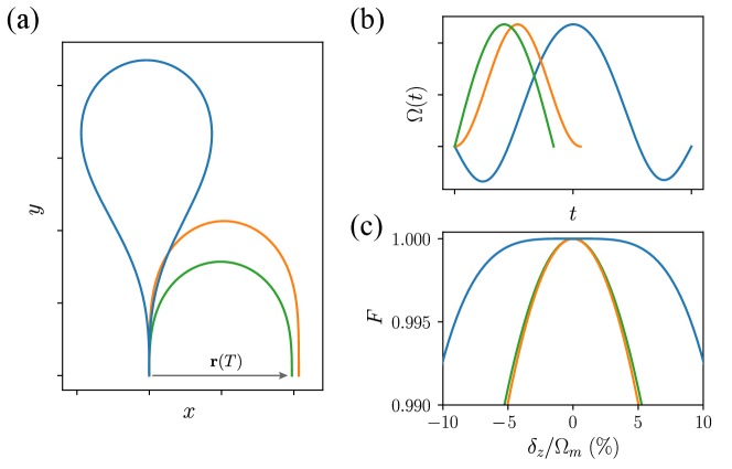
Figure 2: (a) The QEED shows three error curves of RCP (blue), cosine (orange), and sine (green) pulses, corresponding to the pulse waveforms shown in (b). (c) Comparison of the fidelities versus the error strength for different pulse waveforms, as a demonstration of the agreement between the robustness behaviors of different pulses and their error distances.

III.2 Pulse construction protocol

The geometric correspondence helps us understand how the noise affects the qubit dynamics. Therefore, it provides a way to find the conditions of robust evolution and motivates a pulse construction protocol by reverse engineering analytic space curves that satisfy the robustness conditions. The procedure of this construction is summarized as follows: (1) Construct a regular curve that meets certain boundary conditions determined by the target gate operation and robustness conditions such as closeness and vanishing net area; (2) Re-parameterize the curve in terms of the arc-length parameter to make it moving at unit-speed; (3) Scale the length of the curve to fit an optional gate time; (4) Calculate its curvature and torsion to obtain the corresponding robust control pulses. This protocol is illustrated explicitly in previous works, where plane and space curves were used to construct different RCPs [21, 22, 23]. We note that in our generic geometric correspondence, the control pulses are related to signed curvature and singularity-free torsion of the geometric curve, which are obtained by a set of well-chosen continuous Frenet vectors. We demonstrate the pulse construction from space curves and provide a universal plane curve construction for first- and second-order robust pulses in the Supplementary Sec. LABEL:supp-AppendixC and LABEL:supp-AppendixD.

However, even with the constraints given by the theory, it is still challenging to make a good guess of ansatz for the RCPs. In a real quantum computer, the universal gates using RCPs are desired to be generated automatically given the system parameters. Therefore, assistance with numerical search is needed to find the RCPs automatically using the robustness conditions.

Here, we present an analytic-numerical protocol to construct universal error-robust quantum gates that are made automatic. The theory of geometric correspondence gives analytical constraints for robustness, which is added to the objective function to perform constrained optimization using the COCOA algorithm [29]. The protocol is described as follows.

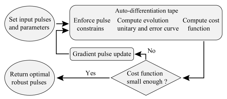
Figure 3: The flow chart of the pulse construction protocol.

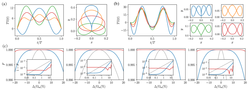
Figure 4: (a) First order robust control pulses $\{R_{1;\bot}^{\pi},R_{1;\bot}^{7\pi/4},R_{1;\bot}^{5\pi/2},R_{1;\bot}^{2\pi}\}$ (blue, orange, green, red) and their corresponding error curves. (b) Extended-robust control pulses $\{R_{\text{ex};\bot}^{\pi},R_{\text{ex};\bot}^{9\pi/4},R_{\text{ex};\bot}^{5\pi/2},R_{\text{ex};\bot}^{2\pi}\}$ (blue, orange, green, red) and their corresponding error curves. (c) Fidelities of the four single-qubit gates $\{X_{\pi},X_{\pi/4},X_{\pi/2},X_{2\pi}\}$ (left to right) realized by the first-order RCPs (blue) as in (a), extended RCPs (red) as in (b), and their cosine pulse counterpart (grey) against detuning noise. Insets are the infidelity versus the relative noise strength for each gate in the log-log scale.

(1) Initialize. Set initial input pulses and other relevant parameters.

(2) Analytic pulse constraints. We apply discrete Fourier series as the generic ansatz of the RCPs, so that we can control the smoothness of the pulses by truncating the Fourier basis while limiting the number of parameters. For pulse amplitude, the Fourier series is multiplied with a sine function to ensure zero boundary values, i.e., zero starting and ending of the pulse waveform. The ansatz of the pulse amplitude and phase takes the form

$$\Omega_{0}(a_{j},\phi_{j};t) =\sin(\frac{\pi t}{T})(a_{0}+\sum_{j=1}^{n}a_{j}\cos(\frac{2\pi j}{T}t+\phi_{j}))$$ (18)

$$\Phi_{0}(b_{j},\psi_{j};t) =b_{0}+\sum_{j=1}^{n}b_{j}\cos(\frac{2\pi j}{T}t+\psi_{j}),$$

where $n$ is the number of Fourier components, which will be set to be $[1,4]$ for different gates shown in this paper. $\{a_{j},\phi_{j},b_{j},\psi_{j}\}$’s are parameters to be optimized. For each input pulse, the corresponding Fourier series is obtained by a Fourier expansion and truncation, and then the expansion function for the amplitude is multiplied with the sine function to obtain a modified pulse.

The reason to choose the Fourier series: 1. few parameters and convenient for experiments; 2. easy to control the smoothness and bandwidth of the pulses; 3. easy to perform pre-distortion according to the transfer function.

(3) Use the modified pulses to compute the dynamics to obtain the evolution operator $U(t)$, as well as the error curve $\mathbf{r}(t)$.

(4) Compute the cost function, which takes the form

$$C=(1-F)+\xi,$$ (19)

where $F$ is the gate fidelity defined in Ref. [45] and $\xi$ is the robustness constraint. When only the first-order robustness is considered, $\xi=\|r(\tau)\|$. Here $\|r(\tau)\|$ is the error distance as defined in  III.1. The robustness against errors in different axes can be achieved by including the error distances of different error curves in the cost function. The auto-differentiation tape records the calculations in (2)-(4).

(5) Make a gradient update of the pulse to minimize $C$.

(6) Go back to step (2) with the updated pulse as input if the cost function is larger than a criterion $\tau$, such as $10^{-5}$.

(7) If $C<\tau$, break the optimization cycle and obtain the optimal robust pulse, which takes the analytical form of Eq. (18).

III.3 Universal set of RCP

Using the pulse construction protocol introduced in the former subsection, we are able to generate RCPs that satisfy the robustness condition provided by the geometric correspondence. As a specific example, we now apply the protocol to search for a set of RCPs that implement X-axis rotation robust against detuning error. Then Eq. (1) now turns into

$$H=\frac{1}{2}\Omega(t)\sigma_{x}+\frac{1}{2}\Delta\sigma_{z}.$$ (20)

We first optimize the control pulses with the first-order robustness around $\Delta=0$. The obtained optimal RCPs are shown in Fig. 4(a) and denoted as $\{R_{1;\bot}^{\pi},R_{1;\bot}^{7\pi/4},R_{1;\bot}^{5\pi/2},R_{1;\bot}^{2\pi}\}$. Here $R_{1;\bot}^{\theta}$ represents the first order RCP for a rotation of angle $\theta$ that can correct errors in its perpendicular directions. We denote the maximum absolute pulse amplitude as $\Omega_{m}=\text{max}\{|\Omega|\}$.

Searching for higher-order robust pulses requires adding more terms associated with the higher-order robustness constraints, e.g., the net-area of the error curve, to the constraint term $\xi$ in the cost function Eq. (19). However, we found that simply adding these constraints hinders the convergence of the algorithm at an unacceptable rate because the computation of these net areas involves complicated integrals over the error curve. We settle this issue by adding new terms to the cost function $C$ with the gate fidelity and error distance at a non-vanishing $\Delta$. Specifically, we use $C=\sum_{j=1,2}(F(\Delta_{j})+\|r(\Delta_{j},\tau)\|)$, where $\Delta_{1}=0$ and $\Delta_{2}$ is chosen to be $\pi/\tau$ according to the experimentalist’s expectation. This ensures the resulting RCPs maintaining high gate fidelities over a broader range of noise amplitude and thus lead to extended robustness. We then obtained a class of extended RCPs denoted as $\{R_{\text{ex};\bot}^{\pi},R_{\text{ex};\bot}^{9\pi/4},R_{\text{ex};\bot}^{5\pi/2},R_{\text{ex};\bot}^{2\pi}\}$ that are made by three cosine functions and the error curves of them have net areas close to zero, as shown in Fig. 4(b). The robustness of the eight RCPs mentioned above is further confirmed by calculating the first few Magnus expansion terms, as shown in the Supplementary Sec. LABEL:supp-AppendixB.

We use the first-order RCPs and the extended RCPs to implement four single-qubit robust gates $\{X_{\pi},X_{\pi/4},X_{\pi/2},X_{2\pi}\}$ ($X_{\theta}$ represents a rotation of angle $\theta$ around x-axis of the Bloch sphere). The first three gates together with robust $Y_{\pi/2}$ gate, a.k.a. applying $R_{1;\bot}^{5\pi/2}$ or $R_{\text{ex};\bot}^{5\pi/2}$ in the Y direction, are elementary single-qubit gates for a universal robust gate set [46], while the $2\pi$ gate is equivalent to the robust dynamical decoupling. We numerically simulate the dynamics of the noisy qubit driven transversely (Eq. 20) and present the gate robustness in Fig. 4(c). Compared with the gates performed by trivial cosine pulses with the same maximal amplitudes of the RCPs, the gates using the first-order RCPs and extended RCPs all exhibit wide high-fidelity plateaus over a significant range of noise amplitude. The gate infidelities exhibit plateaus around $10^{-8}$ within $1\%$ noise region for first-order RCPs and $10^{-5}$ within $15\%$ noise region for extended RCPs. Note that high-fidelity plateaus are a sign of the robustness of the gates.

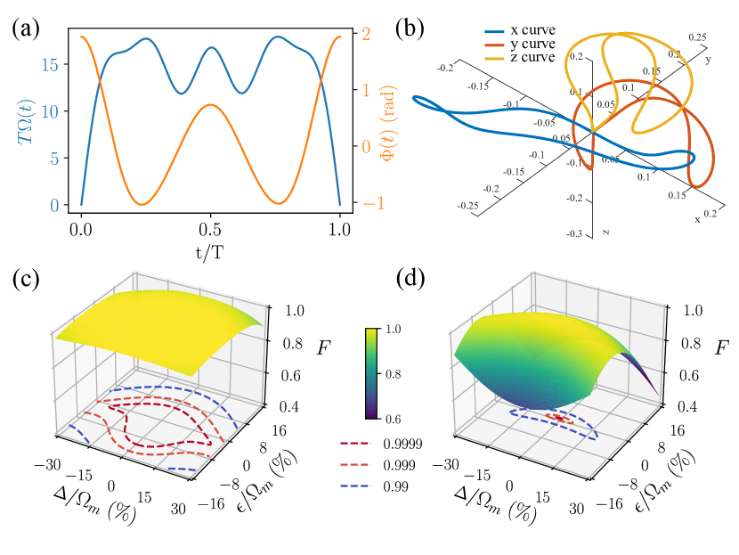
Figure 5: (a) A set of RCPs $R_{1;\text{all}}^{3\pi/2}\{\Omega(t),\Phi(t)\}$ are used to implement robust gate $X_{3\pi/2}$ to correct all errors in x, y, z directions, with the closed x, y, z error curves (blue, orange, yellow) shown in the QEED (b). A comparison of gate fidelity against longitudinal and transverse error $\delta$ and $\epsilon$ using this $R_{1;\text{all}}^{3\pi/2}$ and cosine pulse are shown in (c) and (d).

More general noises on all axes can be corrected simultaneously with XY control with the Hamiltonian in Eq. (5). This works because the robust control in a direction could correct the noise coupled to the other two perpendicular directions, as discussed in the previous section. As a numerical demonstration, we consider both longitudinal and transverse errors in the form of $V=\frac{\Delta}{2}\sigma_{z}+\frac{\epsilon}{2}(\sigma_{x}+\sigma_{y})$, giving rise to the co-existence of x, y and z error curves in the geometric space. Then the robustness constraint in Eq. (19) takes the form $\xi=\sum_{j=x,y,z}\|\mathbf{r}^{j}(\tau)\|$. We apply our protocol to find an RCP $R_{1;\text{all}}^{3\pi/2}$ with only four Fourier components to implement a single-qubit $X_{3\pi/2}$ gate that is robust against errors in all three directions. Although this RCP is solved to generate a robust $3\pi/2$ rotation around the x-axis, its rotation axis can be changed by adding a constant phase while keeping the robustness along the rotation axis and its two perpendicular axes, as demonstrated numerically in the Supplementary Sec. LABEL:supp-AppendixB. As shown in Fig. 5(a) the XY drive has three closed error curves during the gate time. The fidelity landscape of the $X_{3\pi/2}$ gate using the $R_{1;\text{all}}^{3\pi/2}$ and the cosine pulse in the two error dimensions is plotted in Fig. 5(b). The RCP shows a great advantage over the cosine pulse, showing a significant high-fidelity plateau with fidelity above $0.9999$.

IV universal robust quantum gates for realistic qubits

Applying this method to construct universal robust quantum gates for realistic systems, especially in a multi-qubit setup, is not a trivial task. In this section, we demonstrate the method by studying the physical model of gate-defined quantum dots and superconducting transmon qubits.

Without loss of generality, the simulated gate time for all the RCPs is set to be $\tau=50$ ns. The realistic gate time can be arbitrary, and we can always rescale the RCPs in the time domain and maintain their robustness. This is guaranteed by the geometric correspondence since the substitution of $t\rightarrow\alpha t$, $\Omega\rightarrow\Omega/\alpha$ only rescales the length of the error curve and does not change the correspondence such as Eq. (9), as well as the unit-speed properties and robustness conditions of the error curves. In Supplementary Sec. LABEL:supp-AppendixB, we demonstrate this property and provide the parameters for the RCPs involved in the manuscript.

IV.1 Gate-defined quantum dot qubit

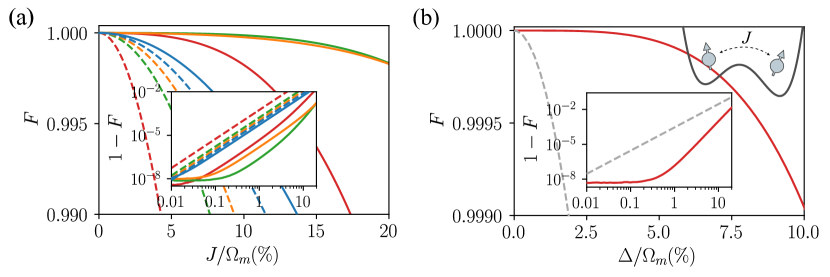
Figure 6: (a) Fidelities of single-qubit gate $\{X_{\pi},X_{\pi/4},X_{\pi/2},\newline X_{2\pi}\}$ (blue, orange, green, red) by RCPs (solid lines) and their cosine counterparts (dashed lines) versus the relative strength of the unwanted coupling $J$. (b) Fidelities of $\sqrt{\text{SWAP}}$ gate by $R_{1;\bot}^{5\pi/2}$ pulse (red) and cosine pulse (grey) versus the Zeeman difference.

First, we consider gate defined double quantum dot system, in which the spin states of electrons serve as qubit [10, 47, 48, 49, 50]. The Hamiltonian is

$$H=\mathbf{B}_{1}\cdot\mathbf{S}_{1}+\mathbf{B}_{2}\cdot\mathbf{S}_{2}+J(\mathbf{S}_{1}\cdot\mathbf{S}_{2}-1/4),$$ (21)

where $\mathbf{S}_{j}=(\sigma_{x,j},\sigma_{y,j},\sigma_{z,j})/2$ and $\mathbf{B}_{j}=(B_{x,j},B_{y,j},B_{z,j})$ are the spin operators and magnetic field acting on qubit $j$, $J$ is the exchange interaction between the spins. We denote the difference of Zeeman splitting between the two qubits as $\Delta=B_{z,2}-B_{z,1}$. Detuning noise from magnetic fluctuations, spin-orbital interaction and residual exchange interaction is one of the major obstacles to further improving the coherence and gate fidelity of such qubits [10, 51].

Single-qubit robust gates.-A single QD is a good two-level system. With detuning noise coupled to a driven QD, the system Hamiltonian takes the same form as Eq. (20). Therefore, the robustness of the pulses driving a single QD can be well described by Fig. 4.

Another source of single-qubit errors is the unwanted coupling between two QDs. The Hamiltonian of such a system with Heisenberg interaction takes the form of Eq. (21). Ideally, the universal single-qubit gates $\{X_{\pi},X_{\pi/4},X_{\pi/2},X_{2\pi}\}$ on the second qubit are given by $I\otimes X_{\theta}$, as the operations on the second qubit shall not affect the first qubit. It is reasonable to assume $J\ll\Delta$, but J cannot be completely turned off during the single-qubit operations by tuning the gate voltage between two QDs [10]. In the eigenbasis, the two subspaces $\text{span}\{|\uparrow\uparrow\rangle,|\tilde{\uparrow\downarrow}\rangle\}$ and $\text{span}\{|\tilde{\downarrow\uparrow}\rangle,|\downarrow\downarrow\rangle\}$ both correspond to the second qubit but are detuned by $J$ in the rotating frame. We tune a magnetic drive $B_{x,2}(t)$ according to the first order RCPs to implement robust X rotations against this detuning resulting from the unwanted coupling. The numerical results demonstrating robust $\{X_{\pi},X_{\pi/4},X_{\pi/2},X_{2\pi}\}$ gates in such double QD system with $\Delta=250$ MHz are shown in Fig. 6(a). Although what we demonstrated here is a partial error cancellation since there is an additional crosstalk error between the two subspaces, which will reduce the gate robustness to some extent, the fidelities are still significantly improved in comparison with the cosine waveform. Further, the crosstalk error can be canceled by appropriately timing and implementing additional correction pulses according to [52, 50], or with more sophisticated RCPs.

Two-qubit robust gates.-Two-qubit $\sqrt{\text{SWAP}}$ gate is commonly used as the entangling gates in the QD system. A perfect $\sqrt{\text{SWAP}}$ can be realized by switching on the exchange coupling in the region where two QDs have zero Zeeman difference—a condition hardly met in experiment either due to the detuning noise or the need for qubit addressability. Note that the entangling originates from the Heisenberg interaction and the Hamiltonian Eq. (21) in the anti-parallel spin states subspace $\text{span}\{|\uparrow\downarrow\rangle,|\downarrow\uparrow\rangle\}$ takes the form

$$H(t)=\frac{1}{2}\left(\begin{array}[]{cc}-J(t)+\Delta&J(t)\\ J(t)&-J(t)-\Delta\end{array}\right).$$ (22)

To implement a $\sqrt{\text{SWAP}}$ gate means to control $J(t)$ to implement $X_{\pi/2}$ operation in this subspace. The waveform of $J(t)$ could be upgraded to a robust pulse $R_{1;\bot}^{5\pi/2}$ in order to fight against the finite Zeeman difference. We numerically solve the time-dependent Schrodinger equation and obtain the results shown in Fig. 6. The robust $\sqrt{\text{SWAP}}$ gate exhibits a high-fidelity plateau, and the infidelity is several orders of magnitude lower than the cosine pulse counterpart in a wide detuning region.

IV.2 Transmon qubit

Single-qubit gates robust to frequency variation.-For a single superconducting transmon with qubit frequency variation, we use the RCPs $\{R_{1}^{\pi},R_{1}^{7\pi/4},R_{1}^{5\pi/2},R_{1}^{2\pi}\}$ found in Fig. 4 to implement robust single-qubit gates $\{X_{\pi},X_{\pi/4},X_{\pi/2},X_{2\pi}\}$. A transmon is usually considered as a three-level system with a moderate anharmonicity between the first and second transitions [53, 54]. With the transverse control field, a transmon could be modeled as

$$H=(\omega+\delta)a^{\dagger}a+\frac{u}{2}a^{\dagger}a^{\dagger}aa+H_{c}(t).$$ (23)

where the control Hamiltonian [54]

$$H_{c}(t)=\frac{1}{2}\xi(t)ae^{i\omega_{d}t}-h.c.$$ (24)

The lowest two levels form the qubit. Here $\omega$, $u$, $a^{\dagger}$, $a$ are the qubit frequency, the anharmonicity, and the creation and annihilation operators of the transmon. $\omega_{d}$ is the frequency of the driving and $\xi(t)$ is the total control waveform. We apply our theory to the dynamics associated with the qubit levels to correct the errors resulting from frequency variation, and use DRAG to suppress the leakage to higher level [55]. So $\xi(t)$ is a sum of RCP $\Omega(t)$ and the corresponding DRAG pulse $i\alpha\dot{\Omega}(t)$. The DRAG parameter $\alpha$ is related to the transmon anharmonicity [55] and takes the numerically optimized value at zero detuning in our simulation.

We set the gate times for $\{X_{\pi},X_{\pi/4},X_{\pi/2},X_{2\pi}\}$ to be $70,50,80$ and $55$ ns such that the maximal pulse amplitudes $\Omega_{m}/2\pi$ are around $27$ MHz, and take the anharmonicity $u/2\pi=-0.26$ GHz. Like previous sections, we use cosine pulses with the same maximal amplitudes for comparison. Our numerical results in Fig. 7(a) illustrate the fidelity plateau over a few MHz of frequency variation for our robust gates. Note that the centers of the fidelity plateau all shift to the left. We conclude the reason to be the AC-Stark shifts associated with the higher levels.

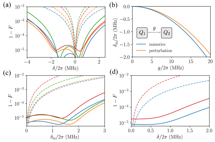
Figure 7: (a) Fidelities of single-qubit gates $\{X_{\pi},X_{\pi/4},X_{\pi/2},\newline X_{2\pi}\}$ (blue, orange, green, red) for a transmon qubit by RCPs (solid) and their cosine counterparts (dashed) versus qubit frequency variation. (b) The strength of ZZ-coupling $\delta_{zz}$ for two capacitively interacting transmons solved numerically (blue) and analytically using perturbation theory (orange). $g$ is the unwanted interaction strength. (c) Fidelities of single-qubit gates $\{X_{\pi},X_{\pi/4},X_{\pi/2},X_{2\pi}\}$ (blue, orange, green, red) for $Q_{2}$ by robust pulses (solid) and their cosine counterparts (dashed) versus residual ZZ-coupling strength caused by unwanted interaction $g$. (d) Fidelity of two-qubit iSWAP (blue) and $\sqrt{\text{iSWAP}}$ (red) for two coupled transmon qubits by RCPs (solid) and their cosine counterparts (dashed) versus the qubits’ frequency difference.

Single-qubit gates robust to unwanted coupling.-In realistic multi-qubit systems, a transmon is unavoidably coupled to another quantum systems, the so-called spectators [14, 56, 39, 57, 58, 59, 60]. This results in qubit frequency splittings or spectrum broadening, giving rise to correlated errors, which becomes a major obstacle for large-scale quantum computing [39]. As a demonstrative example, we consider two directly-coupled transmon qubits (one spectator and one target qubit) with the Hamiltonian

$$H_{0}=\sum_{j=1,2}[\omega_{j}a_{j}^{\dagger}a_{j}+\frac{u_{j}}{2}a_{j}^{\dagger}a_{j}^{\dagger}a_{j}a_{j}]+g(a_{1}^{\dagger}a_{2}+a_{1}a_{2}^{\dagger}),$$ (25)

where $\omega_{j}$ is the qubit frequency, $u_{j}$ is the anharmonicity for the $j$th qubit and $g$ is the interaction strength. Denote the eigenstates of the spectator-target qubit system [14] as $|S,T\rangle$. Up to the second-order perturbation, the effective diagonal Hamiltonian in the subspace $\{\left|00\right\rangle,\left|01\right\rangle\}$ and $\{\left|10\right\rangle,\left|11\right\rangle\}$ is detuned by $\delta_{\text{zz}}$ with $\delta_{\text{zz}}=-\frac{2g^{2}(u_{1}+u_{2})}{(u_{1}+\Delta)(u_{2}-\Delta)}$ and $\Delta=\omega_{2}-\omega_{1}$. This detuning $\delta_{\text{zz}}$ is known as the residual ZZ-coupling. We take $\omega_{1}/2\pi=5.0$ GHz, $\omega_{2}/2\pi=5.5$ GHz, $u_{1}/2\pi=-0.23$ GHz, $u_{2}/2\pi=-0.26$ GHz. The exact $\delta_{\text{zz}}$ obtained by numerical diagonalization and the perturbative one are plotted in Fig. 7(b) as a demonstration of the effectiveness for the perturbative treatment of $\delta_{\text{zz}}$ at small $g$. Our numerical results as shown in Fig. 7(c) illustrate a significant improvement of gate infidelity in the presence of residual ZZ-coupling up to the order of MHz. When ZZ-coupling is vanishing, the infidelity of robust gates remains of the same order as trivial pulses. Here the DRAG control [55] is added as well.

Two-qubit gates.-iSWAP gate is one of the favorable two-qubit entangling gates for quantum computing using transmons [1]. Traditional implementation of the iSWAP gate requires the two qubits to be on resonance. This could be achieved by tuning qubit frequencies, which, however, induces extra flux noise and hence the variation in qubit frequency. To better tune the interaction strength, recent architecture favors tunable couplers [61, 62]. This doesn’t change the effective Hamiltonian in Eq.25, only enabling the control of the coupling strength $g(t)$. To correct the error due to the uncertain frequency difference $\delta$ between the two transmons, we apply RCPs $\{R_{1}^{\pi},R_{1}^{5\pi/2}\}$ on $g(t)$ to implement the robust iSWAP and $\sqrt{\text{iSWAP}}$ gates. We use the qubit settings as in the previous discussion to study the variation of gate infidelities versus $\delta$. The additional ZZ-coupling induced by higher levels of the transmons when activating the iSWAP interaction is omitted in our simulation as it can be canceled by exploiting the tunable coupler and setting a proper gate time [63]. Our numerical results in Fig.7(d) demonstrate a great advantage of RCPs over their cosine counterparts. This control scheme also illustrates the great potential to simplify the experimental tune-ups of qubit frequencies.

V Conclusion and discussion

In summary, the bijective and singularity-free geometric correspondence generates the quantum erroneous evolution diagrams as a graphical analysis for studying the error dynamics of driven quantum systems subject to generic noises. The geometric measures of the errors obtained from the diagrams (Sec.III.1) enable the intuitive and quantitative description of the robustness of arbitrary quantum operation. Furthermore, the framework provides conditions (Sec.II.3) to identify feasible robust control scenarios and allows us to establish an experimental-friendly robust control protocol (Sec.III.2) as a fusion of analytical theory and numerical optimization. John von Neumann famously said: [64]" With four parameters I can fit an elephant, and with five I can make him wiggle his trunk." Here, this protocol exploits no more than four cosine components to construct universal robust quantum gates that can tackle generic errors. These simple pulses will enable low-cost generation and characterization in experiments. The duration of the generated pulses is flexibly adjustable while maintaining robustness as shown in Fig.LABEL:supp-Fig_pulse_rescale. The applications to realistic systems are demonstrated by the numerical simulations on semiconductor spin and superconducting transmon systems, where the gate performance is shown beyond the fault-tolerance threshold over a broad robust plateau. With this simple and versatile protocol, our robust control framework could be applied to experiments immediately and adopted on various physical systems to enhance their robustness in complex noisy environments. The data of the robust control pulses presented in the manuscript and a demonstration of our pulse construction algorithm are available on GitHub [65].

The geometric correspondence is essential Although our discussion in this manuscript focuses on single- and two-qubit systems with multiple quasi-static noises, the framework is directly extensible to multi-qubit systems with complex, time-dependent noise via higher-dimensional geometric correspondence and error curves with modified speeds. And hence it shows a promising prospect in large quantum processors, and will potentially inspire a wave of study on noisy quantum evolution, quantum control and compiling, error mitigation and correction in quantum computers, quantum sensing, metrology, etc. On the other hand, a rigorous mathematical study of the geometric measure theory remains open and is beyond the scope of this work.