Strange partners of the doubly charmed tetraquark $T^{+}_{cc}$

Abstract

The spectroscopic parameters and widths of the axial-vector $T_{cc:s}^{\mathrm{AV}}$ and scalar $T_{cc:s}^{\mathrm{S}}$, $\widetilde{T}_{cc:s}^{\mathrm{S}}$ strange partners of the doubly charmed exotic meson $T_{cc}^{+}$ with the content $cc\overline{u}\overline{s}$, are calculated in the framework of the QCD sum rule method. We model $T_{cc:s}^{\mathrm{AV}}$ as the diquark-antidiquark state composed of axial-vector and scalar components, whereas scalar particles $T_{cc:s}^{\mathrm{S}}$ and $\widetilde{T}_{cc:s}^{\mathrm{S}}$ are built of axial-vector and scalar diquarks, respectively. The masses and current couplings of these tetraquarks are calculated in the context of the two-point sum rule approach by taking into account the quark, gluon and mixed condensates up to dimension $10$. The full width of the state $T_{cc:s}^{\mathrm{AV}}$ is found from analysis of the processes $T_{cc:s}^{\mathrm{AV}}\to D^{0}D_{s}^{\ast+}$ and $T_{cc:s}^{\mathrm{AV}}\to D^{\ast}(2007)^{0}D_{s}^{+}$. Decays to $D^{0}D_{s}^{+}$, $D^{\ast}(2007)^{0}D_{s}^{\ast+}$ and $D^{0}D_{s}^{+}$ mesons are utilized in the case of the scalar tetraquarks $T_{cc:s}^{\mathrm{S}}$ and $\widetilde{T}_{cc:s}^{\mathrm{S}}$, respectively. The partial widths of the aforementioned decays are determined via the strong couplings $g_{1}$, $g_{2}$, $G_{1}$, $G_{2}$ and $\widetilde{G}$, which describe the strong interactions of the particles at the relevant tetraquark-meson-meson vertices. These couplings are computed using the QCD three-point sum rule method, most appropriate for the strong decays under study. The predictions $m=(3995\pm 143)~{}\mathrm{MeV}$ and $\Gamma_{\mathrm{AV}}=(72\pm 13)~{}\mathrm{MeV}$, as well as $m_{\mathrm{S}}=(4128\pm 142)~{}\mathrm{MeV}$, $\Gamma_{\mathrm{S}}=(213\pm 47)~{}\mathrm{MeV}$ and $\widetilde{m}_{\mathrm{S}}=(4035\pm 145)~{}\mathrm{MeV}$ and $\widetilde{\Gamma}_{\mathrm{S}}=(123\pm 32)~{}\mathrm{MeV}$ obtained for the masses and widths of these tetraquarks in the present work can be useful in future experimental investigations of the doubly charmed four-quark resonances.

I Introduction

Recently, the LHCb Collaboration discovered the doubly charmed axial-vector four-quark meson $T_{cc}^{+}$ with content $cc\overline{u}\overline{d}$ Aaij:2021vvq ; LHCb:2021auc . It was observed as a narrow peak in $D^{0}D^{0}\pi^{+}$ invariant mass distribution, and is the first doubly charmed state seen in the experiment. The state $T_{cc}^{+}$ has interesting features: its mass $m_{\exp}=3875.1~{}\mathrm{MeV}+\delta m_{\exp}$, where $\delta m_{\exp}=-273\pm 61\pm 5_{-14}^{+11}~{}\mathrm{KeV}$, is less than two-meson $D^{0}D^{\ast}(2010)^{+}$ threshold , but is very close to it. It is also the longest living exotic meson observed till now, because it has a very small full width $\Gamma=410\pm 165\pm 43_{-38}^{+18}~{}\mathrm{KeV}$.

It is worth noting that the four-quark states $QQ\overline{q}\overline{q}^{\prime}$ containing two heavy quarks $Q$ were already in the center of theoretical investigations Esposito:2013fma ; Navarra:2007yw ; Karliner:2017qjm ; Eichten:2017ffp . The reason is that some of these tetraquarks may be stable against the strong and electromagnetic decays, and therefore can transform to conventional mesons only through weak interaction. Since widths of such particles would be very small, they may be discovered in various exclusive and inclusive processes relatively easily. In the case of tetraquarks $bb\overline{q}\overline{q}^{\prime}$ with different spin-parities and light antidiquark contents $\overline{q}\overline{q}^{\prime}$, this assumption seems is confirmed by numerous studies performed in the context of various models of high energy physics. Thus, stability of the axial-vector tetraquark $T_{bb}^{-}=bb\overline{u}\overline{d}$ was proved in Refs. Navarra:2007yw ; Karliner:2017qjm ; Eichten:2017ffp ; Agaev:2018khe . In Ref. Agaev:2018khe it was demonstrated that the mass of such particle, $m=(10035\pm 260)~{}\mathrm{MeV}$, is below the $B^{-}\overline{B}^{\ast 0}$ and $B^{-}\overline{B}^{0}\gamma$ thresholds. This means that the double-beauty tetraquark $T_{bb}^{-}$ is stable against the strong and radiative decays and dissociates to ordinary mesons only weakly. The full width and mean lifetime of $T_{bb}^{-}$ were evaluated in Refs. Agaev:2018khe ; Agaev:2020mqq using various semileptonic and nonleptonic decay channels of this particle. Results obtained for these parameters, $\Gamma_{\mathrm{full}}=(7.72\pm 1.23)\times 10^{-8}~{}\mathrm{MeV}$ and $\tau=8.53_{-1.18}^{+1.57}~{}\mathrm{fs,}$ are useful for experimental investigations of the tetraquark $T_{bb}^{-}$. Some of other $bb\overline{q}\overline{q}^{\prime}$ states were also identified as stable particles, and their full widths were calculated via allowed weak transformations Xing:2018bqt ; Agaev:2020zag ; Agaev:2020dba ; Agaev:2019lwh .

The doubly charmed tetraquarks $cc\overline{q}\overline{q}^{\prime}$, as interesting objects, were undergone of intensive studies as well Navarra:2007yw ; Karliner:2017qjm ; Eichten:2017ffp ; Du:2012wp ; Wang:2017uld ; Wang:2017dtg ; Braaten:2020nwp ; Cheng:2020wxa ; Meng:2020knc ; Junnarkar:2018twb ; Guo:2021yws ; Padmanath:2022cvl . Thus, the axial-vector tetraquark $cc\overline{u}\overline{d}$ was explored in Ref. Navarra:2007yw in the framework of QCD sum rule method. Properties of the four-quark mesons $cc\overline{q}\overline{q}^{\prime}$ with spin-parities $J^{\mathrm{P}}=0^{-},~{}0^{+},~{}1^{-}$ and $1^{+}$ were analyzed in Ref. Du:2012wp . New investigations of these tetraquarks proved once more the unstable nature of the axial-vector tetraquark $cc\overline{u}\overline{d}$ Karliner:2017qjm ; Eichten:2017ffp ; Wang:2017uld ; Wang:2017dtg ; Braaten:2020nwp ; Cheng:2020wxa . In contrast to these conclusions, studies carried out in the context of the constituent quark model and lattice simulations demonstrated existence of the stable axial-vector tetraquark $cc\overline{u}\overline{d}$ lying $\approx 23~{}\mathrm{MeV}$ below the two-meson threshold Meng:2020knc ; Junnarkar:2018twb .

Detailed investigations of doubly charmed tetraquarks were carried out also in our articles Agaev:2019qqn ; Agaev:2018vag . In the first of these publications, we calculated various parameters of pseudoscalar and scalar states $cc\overline{u}\overline{d}$. Our analyses demonstrated that these four-quark systems are unstable particles and break up to conventional mesons trough strong interactions. Full widths of these particles were evaluated using their kinematically allowed decays to $D^{+}D^{\ast}(2007)^{0}$, $D^{0}D^{\ast}(2010)^{+}$ and $D^{0}D^{+}$ mesons, respectively. Interesting hypothetical pseudoscalar tetraquarks $cc\overline{s}\overline{s}$ and $cc\overline{d}\overline{s}$ carrying two units of electric charge were object of the second paper.

Experimental observation of the resonance $T_{cc}^{+}$ triggered new analyses aimed to explain the measured parameters of this particle Agaev:2021vur ; Feijoo:2021ppq ; Yan:2021wdl ; Fleming:2021wmk ; Agaev:2022ast . In our papers Agaev:2021vur ; Agaev:2022ast , we addressed the relevant problems in the framework of QCD sum rule method. In Ref. Agaev:2021vur , the doubly charmed axial-vector resonance $T_{cc}^{+}$ was treated as the diquark-antidiquark state $cc\overline{u}\overline{d}$. The mass and coupling of this tetraquark were calculated by means of the QCD two-point sum rule approach.

To estimate the full width of $T_{cc}^{+}$, we specified its decay channels and used QCD three-point sum rule method to find the strong couplings at relevant vertices. Because $T_{cc}^{+}$ is a very narrow state, its possible decay modes were objects in numerous analyses. Indeed, $T_{cc}^{+}$ was discovered in the $D^{0}D^{0}\pi^{+}$ mass distribution. One of popular ways to explain such final state is the chain of transformations $T_{cc}^{+}\rightarrow D^{0}D^{\ast+}\rightarrow D^{0}D^{0}\pi^{+}$. But the mass of $T_{cc}^{+}$ is below the $D^{0}D^{\ast+}$ threshold, therefore the process $T_{cc}^{+}\rightarrow D^{0}D^{\ast+}$ is kinematically forbidden, and may proceed only virtually. Alternatively, production of $D^{0}D^{0}\pi^{+}$ may run through a process $T_{cc}^{+}\rightarrow T_{cc;\overline{u}\overline{u}}^{0}\pi^{+}$ where $T_{cc;\overline{u}\overline{u}}^{0}$ is a scalar tetraquark. Then three-meson final state may appear due to the decay $T_{cc;\overline{u}\overline{u}}^{0}\rightarrow D^{0}D^{0}$. To calculate the full width of $T_{cc}^{+}$, we explored also another mode $T_{cc}^{+}\rightarrow\widetilde{T}_{cc;\overline{u}\overline{d}}^{+}\pi^{0}\rightarrow D^{0}D^{+}\pi^{0}$ with $\widetilde{T}_{cc;\overline{u}\overline{d}}^{+}$ being a scalar tetraquark. Results found for the mass and width of the diquark-antidiquark state $T_{cc}^{+}$ are in nice agreement with the LHCb data.

The hadronic molecule model $D^{0}D^{\ast+}$ for the resonance $T_{cc}^{+}$ was examined in Ref. Agaev:2022ast . It turned out that the mass and width of this system exceed experimental data of the LHCb Collaboration. Our studies showed that a preferable assignment for the LHCb resonance $T_{cc}^{+}$ is the diquark-antidiquark model, but because parameters of the molecule $D^{0}D^{\ast+}$ suffer from theoretical uncertainties, we did not exclude the molecule picture for $T_{cc}^{+}$.

The four-quark states containing strange $s$-quark alongside the heavy diquark $cc$ form another interesting class of the doubly charmed particles. These exotic mesons may have diquark-antidiquark or molecular structures. In the context of various methods, masses of the doubly charmed strange tetraquarks with different spin-parities and structures were considered in Refs. Karliner:2021wju ; Chen:2022ros ; Praszalowicz:2022sqx ; Xin:2021wcr ; Ren:2021dsi .

In the present article, we are going to explore features of axial-vector $T_{cc:s}^{\mathrm{AV}}$ and scalar $T_{cc:s}^{\mathrm{S}}$, $\widetilde{T}_{cc:s}^{\mathrm{S}}$ diquark-antidiquark systems $cc\overline{u}\overline{s}$ (in what follows, $T_{\mathrm{AV}}$, $T_{\mathrm{S}}$ and $\widetilde{T}_{\mathrm{S}}$, respectively) by computing their masses, current couplings and widths. We model the tetraquark $T_{\mathrm{AV}}$ as a four-quark meson composed of a heavy axial-vector diquark and light scalar antidiquark. The scalar tetraquarks $T_{\mathrm{S}}$ and $\widetilde{T}_{\mathrm{S}}$ are considered as particles built of the axial-vector and scalar constituents, respectively. To calculate the masses and couplings of these structures, we use QCD two-point sum rules by taking into account various vacuum condensates up to dimension $10$. The width of $T_{\mathrm{AV}}$ is evaluated by considering its $S$-wave decays $T_{\mathrm{AV}}\rightarrow D^{0}D_{s}^{\ast+}$ and $T_{\mathrm{AV}}\rightarrow D^{\ast}(2007)^{0}D_{s}^{+}$. The widths of scalar tetraquarks $T_{\mathrm{S}}$ and $\widetilde{T}_{\mathrm{S}}$ are estimated using their decays to $D^{0}D_{s}^{+}$, $D^{\ast}(2007)^{0}D_{s}^{\ast+}$ and $D^{0}D_{s}^{+}$ mesons, respectively. Partial widths of these processes are determined by the strong couplings $g_{1}$, $g_{2}$, $G_{1}$, $G_{2}$ and $\widetilde{G}$ at tetraquark-meson-meson vertices $T_{\mathrm{AV}}D^{0}D_{s}^{\ast+}$, $T_{\mathrm{AV}}D^{\ast}(2007)^{0}D_{s}^{+}$, $T_{\mathrm{S}}D^{0}D_{s}^{+}$, $T_{\mathrm{S}}D^{\ast}(2007)^{0}D_{s}^{\ast+}$and $\widetilde{T}_{\mathrm{S}}D^{0}D_{s}^{+}$, respectively.

This article is structured in the following manner: In Sec. II, we calculate the mass and current coupling of the tetraquarks $T_{\mathrm{AV}}$, $T_{\mathrm{S}}$ and $\widetilde{T}_{\mathrm{S}}$ in the framework of QCD two-point sum rule method. The strong couplings $g_{1}$, $g_{2}$ and partial widths of the decays $T_{\mathrm{AV}}\rightarrow D^{0}D_{s}^{\ast+}$ and $T_{\mathrm{AV}}\rightarrow D^{\ast}(2007)^{0}D_{s}^{+}$, as well as the full width of $T_{\mathrm{AV}}$ are found in Sec. III. Section IV is devoted to computation of the strong couplings$\ G_{1}$, $G_{2}$ and $\widetilde{G}$ and widths of the tetraquarks $T_{\mathrm{S}}$ and $\widetilde{T}_{\mathrm{S}}$. Section V is reserved for discussion ans concluding notes.

II Spectroscopic parameters of the tetraquarks $T_{\mathrm{AV}}$, $T_{\mathrm{S}}$, and $\widetilde{T}_{\mathrm{S}}$

In this section, we calculate the masses and current couplings of the tetraquarks $T_{\mathrm{AV}}$, $T_{\mathrm{S}}$, and $\widetilde{T}_{\mathrm{S}}$ using the two-point sum rule method Shifman:1978bx ; Shifman:1978by . The key component in the sum rule analysis is an interpolating current for a hadron under consideration. In the diquark-antidiquark model, the four-quark mesons $T_{\mathrm{AV}}$, $T_{\mathrm{S}}$, and $\widetilde{T}_{\mathrm{S}}$ are built of the heavy diquark $cc$ and light antidiquark $\overline{u}\overline{s}$. In the case of the axial-vector state $T_{\mathrm{AV}}$, we suggest that it is composed of the axial-vector diquark $c^{T}C\gamma_{\mu}c$ and scalar antidiquark $\overline{u}\gamma_{5}C\overline{s}^{T}$ with $C$ being the charge conjugation matrix. We take into account that the axial-vector diquark $c_{a}^{T}C\gamma_{\mu}c_{b}$, where $a$ and $b$ are color indices, has a symmetric flavor but an antisymmetric color organization, and its flavor-color structure is $(\mathbf{6}_{f},\overline{\mathbf{3}}_{c})$ Du:2012wp . Then, the color-singlet current $J_{\mu}(x)$ for $T_{\mathrm{AV}}$ can be constructed using the color-triplet light antidiquark field $\overline{u}_{a}\gamma_{5}C\overline{s}_{b}^{T}-\overline{u}_{b}\gamma_{5}C\overline{s}_{a}^{T}$. Because both components of this field lead to identical terms in $J_{\mu}(x)$, it is enough to preserve in calculations one of them. As a result, for the current $J_{\mu}(x)$, we get the following expression

$$J_{\mu}(x)=\left[c_{a}^{T}(x)C\gamma_{\mu}c_{b}(x)\right]\left[\overline{u}_{a}(x)\gamma_{5}C\overline{s}_{b}^{T}(x)\right],$$ (1)

which belongs to the $[\overline{\mathbf{3}}_{c}]_{cc}\otimes[\mathbf{3}_{c}]_{\overline{u}\overline{s}}$ representation of the color group $SU_{c}(3)$.

In the case of the scalar exotic meson $cc\overline{u}\overline{s}$, we consider two structures $T_{\mathrm{S}}$ and $\widetilde{T}_{\mathrm{S}}$ which can describe this tetraquark. We assume that $T_{\mathrm{S}}$ is a scalar tetraquark built of axial-vector components. The interpolating current for such state is given by the expression

$$J(x)=[c_{a}^{T}(x)C\gamma_{\mu}c_{b}(x)][\overline{u}_{a}(x)\gamma^{\mu}C\overline{s}_{b}^{T}(x)],$$ (2)

which is from the antitriplet-triplet representation of the color group $SU_{c}(3)$.

We model $\widetilde{T}_{\mathrm{S}}$ by supposing that it is made of the scalar diquark $c_{a}^{T}C\gamma_{5}c_{b}$ and antidiquark $\overline{u}_{a}\gamma_{5}C\overline{s}_{b}^{T}$. The heavy diquark has symmetric flavor and color structure $(\mathbf{6}_{f},\mathbf{6}_{c})$, i.e., has a color-flavor sextet organization Du:2012wp . Then the light antidiquark should be also symmetric in the color indices $\overline{u}_{a}\gamma_{5}C\overline{s}_{b}^{T}+\overline{u}_{b}\gamma_{5}C\overline{s}_{a}^{T}$. The interpolating current $\widetilde{J}(x)$ of such tetraquark contains relevant diquark and antidiquark fields and has $[\mathbf{6}_{c}]_{cc}\otimes[\overline{\mathbf{6}}_{c}]_{\overline{u}\overline{s}}$ color-structure. In investigations, we employ

$$\widetilde{J}(x)=[c_{a}^{T}(x)C\gamma_{5}c_{b}(x)][\overline{u}_{a}(x)\gamma_{5}C\overline{s}_{b}^{T}(x)],$$ (3)

because components of the antidiquark field generate in the current $\widetilde{J}$ two equal terms.

II.1 The mass and coupling of  $T_{\mathrm{AV}}$

To extract sum rules for the spectroscopic parameters of the tetraquark $T_{\mathrm{AV}}$, we begin from analysis of the correlation function $\Pi_{\mu\nu}(p)$,

$$\Pi_{\mu\nu}(p)=i\int d^{4}xe^{ipx}\langle 0|\mathcal{T}\{J_{\mu}(x)J_{\nu}^{{\dagger}}(0)\}|0\rangle.$$ (4)

First, $\Pi_{\mu\nu}(p)$ should be expressed using the mass $m$ and coupling $f$ of the tetraquark $T_{\mathrm{AV}}$: This expression is the hadronic representation of the $\Pi_{\mu\nu}(p)$ and forms the physical side of the desired sum rules. To this end, we saturate the correlation function $\Pi_{\mu\nu}(p)$ with a complete set of states with quantum numbers $J^{\mathrm{P}}=1^{+}$ and perform the integration over $x$ in Eq. (4),

$$\Pi_{\mu\nu}^{\mathrm{Phys}}(p)=\frac{\langle 0|J_{\mu}|T_{\mathrm{AV}}(p,\epsilon)\rangle\langle T_{\mathrm{AV}}(p,\epsilon)|J_{\nu}^{\dagger}|0\rangle}{m^{2}-p^{2}}+\cdots.$$ (5)

We write down the contribution arising from the ground-state particle $T_{\mathrm{AV}}$ explicitly, and denote ones due to higher resonances and continuum states by the dots.

The function $\Pi_{\mu\nu}^{\mathrm{Phys}}(p)$ can be simplified using the matrix element,

$$\langle 0|J_{\mu}|T_{\mathrm{AV}}(p,\epsilon)\rangle=fm\epsilon_{\mu},$$ (6)

where $\epsilon_{\mu}$ is the polarization vector of $T_{\mathrm{AV}}$. It is not difficult to demonstrate that in terms of $m$ and $f$ the function $\Pi_{\mu\nu}^{\mathrm{Phys}}(p)$ takes the following form:

$$\Pi_{\mu\nu}^{\mathrm{Phys}}(p)=\frac{m^{2}f^{2}}{m^{2}-p^{2}}\left(-g_{\mu\nu}+\frac{p_{\mu}p_{\nu}}{m^{2}}\right)+\cdots.$$ (7)

The QCD side of the sum rules $\Pi_{\mu\nu}^{\mathrm{OPE}}(p)$ has to be computed in the operator product expansion ($\mathrm{OPE}$) with some fixed accuracy. The function $\Pi_{\mu\nu}^{\mathrm{OPE}}(p)$ can be obtained by inserting the explicit form of the interpolating current $J_{\mu}(x)$ into Eq. (4), and contracting corresponding heavy and light quark fields. After these operations, we get

$$\Pi_{\mu\nu}^{\mathrm{OPE}}(p)=i\int d^{4}xe^{ipx}\mathrm{Tr}\left[\gamma_{5}\widetilde{S}_{s}^{b^{\prime}b}(-x)\right.$$

$$\left.\times\gamma_{5}S_{u}^{a^{\prime}a}(-x)\right]\left\{\mathrm{Tr}\left[\gamma_{\nu}\widetilde{S}_{c}^{ba^{\prime}}(x)\gamma_{\mu}S_{c}^{ab^{\prime}}(x)\right]\right.$$

$$\left.-\mathrm{Tr}\left[\gamma_{\nu}\widetilde{S}_{c}^{aa^{\prime}}(x)\gamma_{\mu}S_{c}^{bb^{\prime}}(x)\right]\right\}.$$ (8)

In Eq. (8), $S_{c}^{ab}(x)$ and $S_{q}^{ab}(x)$ are the $c$ and $q(u,s)$-quark propagators: their analytic expressions were presented in Ref. Agaev:2020zad . We have also introduced the notation

$$\widetilde{S}_{c(q)}(x)=CS_{c(q)}^{T}(x)C.$$ (9)

The QCD sum rules are obtained by equating the invariant amplitudes which correspond to the same Lorentz structures both in $\Pi_{\mu\nu}^{\mathrm{Phys}}(p)$ and $\Pi_{\mu\nu}^{\mathrm{OPE}}(p)$. The amplitudes corresponding to the structures $\sim g_{\mu\nu}$ do not receive contributions from the spin-$0$ particles, therefore, they are suitable for our purposes. Having denoted these invariant amplitudes by $\Pi^{\mathrm{Phys}}(p^{2})$ and $\Pi^{\mathrm{OPE}}(p^{2})$, respectively, and equating them, we find an expression which is convenient for further processing. First, we encounter here problems connected with necessity to suppress the contributions of the higher resonances and continuum states. For these purposes, we make use of the Borel transformation in the sum rule equality. Afterwards, employing the assumption about quark-hadron duality, it is possible to subtract these effects from the obtained expression. After these manipulations, the sum rule equality acquires dependence on the Borel $M^{2}$ and continuum threshold $s_{0}$ parameters.

It is evident that the Borel transformation of $\Pi^{\mathrm{Phys}}(p^{2})$ is trivial. The Borel transformation and continuum subtraction convert the invariant amplitude $\Pi^{\mathrm{OPE}}(p^{2})$ to the form,

$$\Pi(M^{2},s_{0})=\int_{\mathcal{M}^{2}}^{s_{0}}ds\rho^{\mathrm{OPE}}(s)e^{-s/M^{2}}+\Pi(M^{2}),$$ (10)

where $\mathcal{M}=2m_{c}+m_{s}$. In numerical computations, we set $m_{u}=0$ and $m_{s}^{2}=0$, but take into account terms proportional to $m_{s}$. In Eq. (10), $\rho^{\mathrm{OPE}}(s)$ is the two-point spectral density computed as the imaginary part of the correlation function. The second component of the invariant amplitude $\Pi(M^{2})$ includes nonperturbative contributions extracted directly from $\Pi_{\mu\nu}^{\mathrm{OPE}}(p)$. We calculate $\Pi(M^{2},s_{0})$ by taking into account the nonperturbative terms up to dimension $10$. Explicit expression of $\Pi(M^{2},s_{0})$ is rather cumbersome, therefore we do not provide it here.

The sum rules for $m$ and $f$ read

$$m^{2}=\frac{\Pi^{\prime}(M^{2},s_{0})}{\Pi(M^{2},s_{0})},$$ (11)

and

$$f^{2}=\frac{e^{m^{2}/M^{2}}}{m^{2}}\Pi(M^{2},s_{0}),$$ (12)

where $\Pi^{\prime}(M^{2},s_{0})=d\Pi(M^{2},s_{0})/d(-1/M^{2})$.

The formulas in Eqs. (11) and (12) depend on the various quark, gluon and mixed condensates. They are universal quantities extracted from numerous analyses:

$$\langle\overline{q}q\rangle=-(0.24\pm 0.01)^{3}~{}\mathrm{GeV}^{3},\ \langle\overline{s}s\rangle=(0.8\pm 0.1)\langle\overline{q}q\rangle,$$

$$\langle\overline{q}g_{s}\sigma Gq\rangle=m_{0}^{2}\langle\overline{q}q\rangle,\ \langle\overline{s}g_{s}\sigma Gs\rangle=m_{0}^{2}\langle\overline{s}s\rangle,$$

$$m_{0}^{2}=(0.8\pm 0.2)~{}\mathrm{GeV}^{2}$$

$$\langle\frac{\alpha_{s}G^{2}}{\pi}\rangle=(0.012\pm 0.004)~{}\mathrm{GeV}^{4},$$

$$\langle g_{s}^{3}G^{3}\rangle=(0.57\pm 0.29)~{}\mathrm{GeV}^{6},$$

$$m_{s}=93_{-5}^{+11}~{}\mathrm{MeV},\ m_{c}=(1.27\pm 0.02)~{}\mathrm{GeV}.$$ (13)

We also added the masses of $c$ and $s$ quarks to this list.

It is known that the Borel and continuum threshold parameters, $M^{2}$ and $s_{0}$, are auxiliary quantities of calculations, which have to satisfy some constraints imposed on $\Pi(M^{2},s_{0})$ by the dominance of the pole contribution ($\mathrm{PC}$) and convergence of the $\mathrm{OPE}$. We use the following definition for $\mathrm{PC}$:

$$\mathrm{PC}=\frac{\Pi(M^{2},s_{0})}{\Pi(M^{2},\infty)}.$$ (14)

The restriction on $\mathrm{PC}$ is necessary to fix the maximum value of the Borel parameter. The low boundary of the window for the Borel parameter is obtained from the convergence of the $\mathrm{OPE}$. To this end, we employ the expression

$$R(M^{2})=\frac{\Pi^{\mathrm{DimN}}(M^{2},s_{0})}{\Pi(M^{2},s_{0})},$$ (15)

where $\Pi^{\mathrm{DimN}}(M^{2},s_{0})$ is the contribution of the last three terms in $\mathrm{OPE}$, i.e., $\mathrm{DimN=Dim(8+9+10)}$.

Apart from these constraints, the region for $M^{2}$ should lead to stable predictions for extracted physical quantities. Our computations prove that the regions for $M^{2}$ and $s_{0}$,

$$M^{2}\in[3,4.5]~{}\mathrm{GeV}^{2},\ s_{0}\in[20.5,21.5]~{}\mathrm{GeV}^{2},$$ (16)

satisfy all restrictions mentioned above. In fact, in these regions, on average in $s_{0}$, the pole contribution changes within the limits:

$$0.79\geq\mathrm{PC}\geq 0.49.$$ (17)

At $M^{2}=3~{}\mathrm{GeV}^{2}$, the contributions to $\Pi(M^{2},s_{0})$ of the last three terms in $\mathrm{OPE}$ is less than $0.01$.

In Fig. 1, we plot the dependence of the mass $m$ of the tetraquark $T_{\mathrm{AV}}$ on $M^{2}$ and $s_{0}$. It is clear, that the window for $M^{2}$, where parameters of $T_{\mathrm{AV}}$ are extracted, can be considered as a relatively stable plateau. Nevertheless, one sees a residual dependence of $m$ on the Borel parameter $M^{2}$. This effect allows one to find ambiguities of the sum rule calculations. Another source of the theoretical uncertainties is the continuum threshold parameter $s_{0}$. The region for $s_{0}$ has to meet the constraints coming from the dominance of $\mathrm{PC}$ and convergence of the $\mathrm{OPE}$. The parameter $\sqrt{s_{0}}$ bears also information on the mass of the $T_{\mathrm{AV}}$ tetraquark’s first radial excitation.

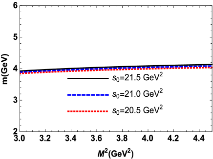
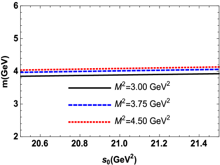
Figure 1: Mass $m$ of the tetraquark $T_{\mathrm{AV}}$ as a function of the Borel parameter $M^{2}$ (left), and the continuum threshold parameter $s_{0}$ (right).

Our results for the spectral parameters of the tetraquark $T_{\mathrm{AV}}$ read

$$m = (3995\pm 143)~{}\mathrm{MeV},$$

$$f = (2.4\pm 0.5)\times 10^{-3}~{}\mathrm{GeV}^{4}.$$ (18)

The predictions for the mass $m$ and coupling $f$ are obtained as average of results for these quantities in the working windows (16). These values correspond to the sum rules’ predictions approximately at middle of these regions, i.e., to results at $M^{2}=3.5~{}\mathrm{GeV}^{2}$ and $s_{0}=21~{}\mathrm{GeV}^{2}$, where $\mathrm{PC}\approx 0.65$ guarantees the ground-state nature of $T_{\mathrm{AV}}$. As it has been noted above, $\sqrt{s_{0}}-m\geq 480~{}\mathrm{MeV}$ allows us to estimate the mass of the excited tetraquark as $m^{\ast}\approx(m+480)~{}\mathrm{MeV}$, which is reasonable for double-heavy tetraquarks.

II.2 Parameters of the tetraquarks $T_{\mathrm{S}}$ and $\widetilde{T}_{\mathrm{S}}$

To find the mass $m_{\mathrm{S}}$ and current coupling $f_{\mathrm{S}}$ of the scalar tetraquark $T_{\mathrm{S}}$, we start from the correlation function $\Pi(p)$

$$\Pi(p)=i\int d^{4}xe^{ipx}\langle 0|\mathcal{T}\{J(x)J^{{\dagger}}(0)\}|0\rangle,$$ (19)

where the current $J(x)$ is given by Eq. (2). In terms of the tetraquark’s physical parameters, $\Pi(p)$ is determined by the expression,

$$\Pi^{\mathrm{Phys}}(p)=\frac{\langle 0|J|T_{\mathrm{S}}(p)\rangle\langle T_{\mathrm{S}}(p)|J^{\dagger}|0\rangle}{m_{\mathrm{S}}^{2}-p^{2}}+\cdots.$$ (20)

The function $\Pi^{\mathrm{Phys}}(p)$ can be rewritten by employing the matrix element,

$$\langle 0|J|T_{\mathrm{S}}(p)\rangle=m_{\mathrm{S}}f_{\mathrm{S}}.$$ (21)

Then, it is easy to see that in terms of the parameters $m_{\mathrm{S}}$ and $f_{\mathrm{S}}$ the $\Pi^{\mathrm{Phys}}(p)$ has the form,

$$\Pi^{\mathrm{Phys}}(p)=\frac{m_{\mathrm{S}}^{2}f_{\mathrm{S}}^{2}}{m_{\mathrm{S}}^{2}-p^{2}}+\cdots.$$ (22)

To obtain the QCD side of the sum rules, $\Pi^{\mathrm{OPE}}(p)$, we insert the interpolating current $J(x)$ into Eq. (19), and contract the relevant quark fields. After these manipulations, we get

$$\Pi^{\mathrm{OPE}}(p)=i\int d^{4}xe^{ipx}\mathrm{Tr}\left[\gamma_{\mu}\widetilde{S}_{s}^{b^{\prime}b}(-x)\right.$$

$$\left.\times\gamma_{\nu}S_{u}^{a^{\prime}a}(-x)\right]\left\{\mathrm{Tr}\left[\gamma^{\nu}\widetilde{S}_{c}^{aa^{\prime}}(x)\gamma^{\mu}S_{c}^{bb^{\prime}}(x)\right]\right.$$

$$\left.-\mathrm{Tr}\left[\gamma^{\nu}\widetilde{S}_{c}^{ba^{\prime}}(x)\gamma^{\mu}S_{c}^{ab^{\prime}}(x)\right]\right\}.$$ (23)

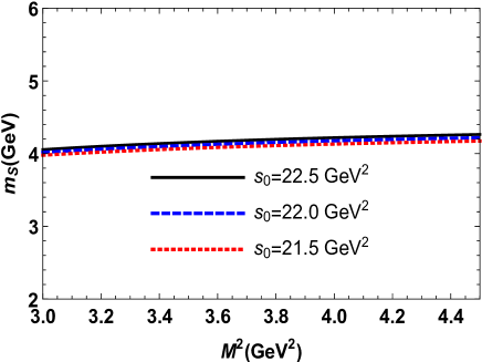
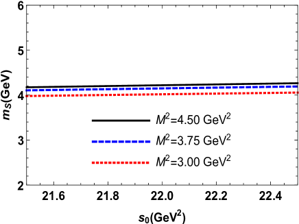
Figure 2: Dependence of the $T_{\mathrm{S}}$ tetraquark’s mass $m_{\mathrm{S}}$ on the Borel parameter $M^{2}$ (left), and on the continuum threshold parameter $s_{0}$ (right).

Because the remaining operations with the correlation function $\Pi^{\mathrm{OPE}}(p)$ are standard ones, we omit the further details and provide only the final results for the mass $m_{\mathrm{S}}$ and coupling $f_{\mathrm{S}}$:

$$m_{\mathrm{S}} = (4128\pm 142)~{}\mathrm{MeV},$$

$$f_{\mathrm{S}} = (3.84\pm 0.34)\times 10^{-3}~{}\mathrm{GeV}^{4}.$$ (24)

Let us note that the values of $m_{\mathrm{S}}$ and $f_{\mathrm{S}}$ are found utilizing for the parameters $M^{2}$ and $s_{0}$ working regions

$$M^{2}\in[3,4.5]~{}\mathrm{GeV}^{2},\ s_{0}\in[21.5,22.5]~{}\mathrm{GeV}^{2}.$$ (25)

In these regions the pole contribution varies within boundaries

$$0.69\geq\mathrm{PC}\geq 0.51,$$ (26)

and $R(3~{}\mathrm{GeV}^{2})<0.01$. The behavior of $m_{\mathrm{S}}$ as a function of $M^{2}$ and $s_{0}$ is depicted in Fig. 2.

Similar analysis for the tetraquark $\widetilde{T}_{\mathrm{S}}$ gives

$$\widetilde{\Pi}^{\mathrm{OPE}}(p)=i\int d^{4}xe^{ipx}\mathrm{Tr}\left[\gamma_{5}\widetilde{S}_{s}^{b^{\prime}b}(-x)\right.$$

$$\left.\times\gamma_{5}S_{u}^{a^{\prime}a}(-x)\right]\left\{\mathrm{Tr}\left[\gamma_{5}\widetilde{S}_{c}^{aa^{\prime}}(x)\gamma_{5}S_{c}^{bb^{\prime}}(x)\right]\right.$$ (27)

$$\left.+\mathrm{Tr}\left[\gamma_{5}\widetilde{S}_{c}^{ba^{\prime}}(x)\gamma_{5}S_{c}^{ab^{\prime}}(x)\right]\right\}.$$ (28)

The spectroscopic parameters of $\widetilde{T}_{\mathrm{S}}$ are equal to

$$\widetilde{m}_{\mathrm{S}} = (4035\pm 145)~{}\mathrm{MeV},$$

$$\widetilde{f}_{\mathrm{S}} = (7.7\pm 1.2)\times 10^{-3}~{}\mathrm{GeV}^{4}.$$ (29)

To extract $\widetilde{m}_{\mathrm{S}}$ and $\widetilde{f}_{\mathrm{S}}$ , we used the windows Eq. (16) for the parameters $M^{2}$ and $s_{0}$, which satisfy all of the sum rule constraints in this case as well.

III Width of the tetraquark $T_{\mathrm{AV}}$

In the previous section, we have calculated the masses and couplings of the tetraquarks $T_{\mathrm{AV}}$, $T_{\mathrm{S}}$ and $\widetilde{T}_{\mathrm{S}}$. This information forms a basis to determine the kinematically allowed decay channels of these particles. In the case of the tetraquark $T_{\mathrm{AV}}$ the channels $T_{\mathrm{AV}}\rightarrow D^{0}D_{s}^{\ast+}$ and $T_{\mathrm{AV}}\rightarrow D^{\ast}(2007)^{0}D_{s}^{+}$ are its $S$-wave modes, thresholds for which equal to $\approx 3975~{}\mathrm{MeV}$ and $3977~{}\mathrm{MeV}$, respectively. We calculate the full width of $T_{\mathrm{AV}}$ by taking into account these two channels.

It is worth noting, that we use central value of the mass $m$. But sum rule computations depend on auxiliary parameters $M^{2}$ and $s_{0}$, which restrict precision of the method by generating uncertainties in extracted physical observables. Thus, the maximal predicted value for $m$ is $4138~{}\mathrm{MeV}$ which, however does not affect considerably our result for its full widths. The reason is that even for such $m$ other strong decays of $T_{\mathrm{AV}}$, for instance, $P$-wave modes $T_{\mathrm{AV}}\rightarrow D^{0}D_{s0}^{\ast}(2317)^{+}$ or $T_{\mathrm{AV}}\rightarrow D_{0}^{\ast}(2400)^{0}D_{s}^{+}$ are kinematically forbidden processes because $4138~{}\mathrm{MeV}$ is below relevant two-meson thresholds.

At the $m$ less than the limit $3975~{}\mathrm{MeV}$ the axial-vector state $T_{\mathrm{AV}}$ cannot decay to $D^{0}D_{s}^{\ast+}$ and $D^{\ast}(2007)^{0}D_{s}^{+}$. The process $T_{\mathrm{AV}}\rightarrow D^{0}D^{0}K^{+}$, analog of $T_{cc}^{+}\rightarrow D^{0}D^{0}\pi^{+}$, could not also take place: A threshold for this decay $4224~{}\mathrm{MeV}$ is significantly larger than $3975~{}\mathrm{MeV}$. Therefore, at $m<3975~{}\mathrm{MeV}$ the tetraquark $T_{\mathrm{AV}}$ becomes a strong-interaction stable particle, which is excluded by the experimental data of the LHCb Collaboration and theoretical analyses of diquark masses. In fact, the axial-vector states $T_{cc}^{+}=cc\overline{u}\overline{d}$ and $T_{\mathrm{AV}}=cc\overline{u}\overline{s}$ contain the same heavy diquark $c^{T}C\gamma_{\mu}c$ and ”good” light scalar antidiquarks $\overline{u}\gamma_{5}C\overline{d}^{T}$ and $\overline{u}\gamma_{5}C\overline{s}^{T}$ in $(\mathbf{3}_{f},\mathbf{3}_{c})$ flavor-color representations, respectively. The mass splitting $\delta$ between ”good” $J^{\mathrm{P}}=0^{+}$ diquarks $us$ and $ud$ was analyzed in Ref. Burden:1996nh and found equal to $145~{}\mathrm{MeV}$. This gap leads to the mass of $T_{\mathrm{AV}}$ approximately around of $4020~{}\mathrm{MeV}$. Our prediction for $m$, as well as for the $T_{\mathrm{AV}}-T_{cc}^{+}$ mass splitting $\Delta=120~{}\mathrm{MeV}$ are close to these estimates. Thus, the experimental-theoretical analyses rule out the small mass region for $T_{\mathrm{AV}}$, and confirm its unstability against strong decays to conventional open-charmed mesons.

III.1 Decay $T_{\mathrm{AV}}\rightarrow D^{0}D_{s}^{\ast+}$

Here, we consider in a detailed form the process $T_{\mathrm{AV}}\rightarrow D^{0}D_{s}^{\ast+}$. The partial width of this decay contains various physical parameters of the initial and final particles, such as their masses and decay constants. These parameters are known from other sources or have been computed in the present article.

The partial width depends also on the strong interaction’s coupling $g_{1}$ of the corresponding tetraquark and mesons at the vertex $T_{\mathrm{AV}}D^{0}D_{s}^{\ast+}$. It is convenient to determine $g_{1}$ by means of the QCD three-point sum rule method. To this end, we analyze the correlation function

$$\Pi_{\mu\nu}(p,p^{\prime})=i^{2}\int d^{4}xd^{4}ye^{i(p^{\prime}y-px)}\langle 0|\mathcal{T}\{J_{\nu}^{D_{s}^{\ast}}(y)$$

$$\times J^{D^{0}}(0)J_{\mu}^{\dagger}(x)\}|0\rangle,$$ (30)

where $J_{\mu}(x)$,$\ J_{\nu}^{D_{s}^{\ast}}(y)$ and $J^{D^{0}}(0)$ are the interpolating currents for the tetraquark $T_{\mathrm{AV}}$, the vector $D_{s}^{\ast+}$ and pseudoscalar $D^{0}$ mesons, respectively. The four-momenta of $T_{\mathrm{AV}}$ and $D_{s}^{\ast+}$ are denoted by $p$ and $p^{\prime}$, then momentum of the meson $D^{0}$ is equal to $q=p-p^{\prime}$.

The $J_{\mu}(x)$ is determined by Eq. (1), whereas for currents of two final-state mesons, we use

$$\ J_{\nu}^{D_{s}^{\ast}}(x) = \overline{s}_{j}(x)\gamma_{\nu}c_{j}(x),$$

$$J^{D^{0}}(x) = \overline{u}_{i}(x)i\gamma_{5}c_{i}(x),$$ (31)

where $i$ and $j$ are color indices.

To continue our study in the framework of the sum rule method, we calculate the correlation function $\Pi_{\mu\nu}(p,p^{\prime})$ by employing the physical parameters of the particles involved into this process. For the physical side of the sum rule, $\Pi_{\mu\nu}^{\mathrm{Phys}}(p,p^{\prime})$, we obtain

$$\Pi_{\mu\nu}^{\mathrm{Phys}}(p,p^{\prime})=\frac{\langle 0|J_{\nu}^{D^{\ast}}|D_{s}^{\ast+}(p^{\prime},\varepsilon^{\prime})\rangle\langle 0|J^{D^{0}}|D^{0}(q)\rangle}{(p^{\prime 2}-m_{D_{s}^{\ast}}^{2})(q^{2}-m_{D}^{2})}$$

$$\times\frac{\langle D^{0}(q)D_{s}^{\ast+}(p^{\prime},\varepsilon^{\prime})|T_{\mathrm{AV}}(p,\epsilon)\rangle\langle T_{\mathrm{AV}}(p,\epsilon)|J_{\mu}^{\dagger}|0\rangle}{(p^{2}-m^{2})}+\cdots,$$

(32)

where $m_{D_{s}^{\ast}}$ and $m_{D}$ are the masses of the mesons $D_{s}^{\ast+}$ and $D^{0}$, respectively. To derive this expression, we separate the contributions of the ground-state particles from the effects of the higher resonances and continuum states in Eq. (30). Hence, in Eq. (32), the ground-state term is written down explicitly, whereas ellipses stand for the other contributions.

The function $\Pi_{\mu\nu}^{\mathrm{Phys}}(p,p^{\prime})$ can be simplified by introducing the $D_{s}^{\ast+}$ and $D^{0}$ mesons’ matrix elements

$$\langle 0|J_{\nu}^{D^{\ast}}|D_{s}^{\ast+}(p^{\prime},\varepsilon^{\prime})\rangle = m_{D_{s}^{\ast}}f_{D_{s}^{\ast}}\varepsilon_{\nu}^{\prime},\$$

$$\langle 0|J^{D^{0}}|D^{0}\rangle = \frac{m_{D}^{2}f_{D}}{m_{c}},$$ (33)

with $f_{D_{s}^{\ast}}$ and $f_{D}$ being their decay constants. Here, $\varepsilon_{\nu}^{\prime}$ is the polarization vector of the meson $D_{s}^{\ast+}$.

The matrix element of the vertex $T_{\mathrm{AV}}D^{0}D_{s}^{\ast+}$ can be modeled in the form

$$\langle D^{0}(q)D_{s}^{\ast+}(p^{\prime},\varepsilon^{\prime})|T_{\mathrm{AV}}(p,\epsilon)\rangle=g_{1}(q^{2})\left[\left(p\cdot p^{\prime}\right)\left(\epsilon\cdot\varepsilon^{\prime\ast}\right)\right.$$

$$\left.-\left(p^{\prime}\cdot\epsilon\right)\left(p\cdot\varepsilon^{\prime\ast}\right)\right],$$ (34)

where we denote the strong coupling at $T_{\mathrm{AV}}D^{0}D_{s}^{\ast+}$ by $g_{1}(q^{2})$. Then, one can easily find that

$$\Pi_{\mu\nu}^{\mathrm{Phys}}(p,p^{\prime})=g_{1}(q^{2})\frac{m_{D_{s}^{\ast}}f_{D_{s}^{\ast}}m_{D}^{2}f_{D}fm}{m_{c}(p^{2}-m^{2})(q^{2}-m_{D}^{2})}$$

$$\times\frac{1}{(p^{\prime 2}-m_{D_{s}^{\ast}}^{2})}\left(\frac{m^{2}+m_{D_{s}^{\ast}}^{2}-q^{2}}{2}g_{\mu\nu}-p_{\nu}p_{\mu}^{\prime}\right)+\cdots.$$

(35)

The double Borel transformation of the correlation function over the variables $-p^{2}$ and $-p^{\prime 2}$ is determined by the expression

$$\mathcal{B}\Pi_{\mu\nu}^{\mathrm{Phys}}(p,p^{\prime})=g_{1}(q^{2})\frac{m_{D_{s}^{\ast}}f_{D_{s}^{\ast}}m_{D}^{2}f_{D}fm}{m_{c}(q^{2}-m_{D}^{2})}e^{-m^{2}/M_{1}^{2}}$$

$$\times e^{-m_{D_{s}^{\ast}}^{2}/M_{2}^{2}}\left(\frac{m^{2}+m_{D_{s}^{\ast}}^{2}-q^{2}}{2}g_{\mu\nu}-p_{\mu}p_{\nu}^{\prime}\right)+\cdots.$$

The function $\mathcal{B}\Pi_{\mu\nu}^{\mathrm{Phys}}(p,p^{\prime})$ has two Lorentz structures which are proportional to $g_{\mu\nu}$ and $p_{\nu}p_{\mu}^{\prime}$. In our analysis, we work with the Borel transformation of the invariant amplitude $\Pi^{\mathrm{Phys}}(p^{2},p^{\prime 2},q^{2})$ which corresponds to the structure $\sim g_{\mu\nu}$.

To derive the QCD side of the three-point sum rule, we calculate $\Pi_{\mu\nu}(p,p^{\prime})$ using the quark propagators, and obtain

$$\Pi_{\mu\nu}^{\mathrm{OPE}}(p,p^{\prime})=i^{3}\int d^{4}xd^{4}ye^{i(p^{\prime}y-px)}$$

$$\times\left\{\mathrm{Tr}\left[\gamma_{\nu}S_{c}^{ja}(y-x)\gamma_{\mu}\widetilde{S}_{c}^{ib}(-x)\gamma_{5}\widetilde{S}_{u}^{ai}(x)\gamma_{5}\right.\right.$$

$$\left.\times S_{s}^{bj}(x-y)\right]-\mathrm{Tr}\left[\gamma_{\nu}S_{c}^{jb}(y-x)\gamma_{\mu}\widetilde{S}_{c}^{ia}(-x)\right.$$

$$\left.\left.\times\gamma_{5}\widetilde{S}_{u}^{ai}(x)\gamma_{5}S_{s}^{bj}(x-y)\right]\right\}.$$ (37)

The correlation function $\Pi_{\mu\nu}^{\mathrm{OPE}}(p,p^{\prime})$ is computed by taking into account the nonperturbative contributions up to dimension $6$. It contains the same Lorentz structures as $\Pi_{\mu\nu}^{\mathrm{Phys}}(p,p^{\prime})$. Let us denote by $\Pi^{\mathrm{OPE}}(p^{2},p^{\prime 2},q^{2})$ the invariant amplitude that corresponds to the term proportional to $g_{\mu\nu}$ in $\Pi_{\mu\nu}^{\mathrm{OPE}}(p,p^{\prime})$. The double Borel transformation, $\mathcal{B}\Pi^{\mathrm{OPE}}(p^{2},p^{\prime 2},q^{2})$, establishes the second component of the sum rule. Having equated $\mathcal{B}\Pi^{\mathrm{OPE}}(p^{2},p^{\prime 2},q^{2})$ and $\mathcal{B}\Pi^{\mathrm{Phys}}(p^{2},p^{\prime 2},q^{2})$, and carried out the continuum subtraction, we derive the sum rule for the strong coupling $g_{1}(q^{2})$.

The Borel transformed and subtracted amplitude $\Pi^{\mathrm{OPE}}(p^{2},p^{\prime 2},q^{2})$ can be expressed by means of the spectral density $\widetilde{\rho}(s,s^{\prime},q^{2})$ which is proportional to the relevant imaginary part of the $\Pi_{\mu\nu}^{\mathrm{OPE}}(p,p^{\prime})$

$$\Pi(\mathbf{M}^{2},\mathbf{s}_{0},q^{2})=\int_{\mathcal{M}^{2}}^{s_{0}}ds\int_{(m_{c}+m_{s})^{2}}^{s_{0}^{\prime}}ds^{\prime}\rho(s,s^{\prime},q^{2})$$

$$\times e^{-s/M_{1}^{2}}e^{-s^{\prime}/M_{2}^{2}}.$$ (38)

The Borel and continuum threshold parameters are denoted in Eq. (38) by $\mathbf{M}^{2}=(M_{1}^{2},\ M_{2}^{2})$ and $\mathbf{s}_{0}=(s_{0},\ s_{0}^{\prime})$, respectively. Then, the sum rule for $g_{1}(q^{2})$ reads

$$g_{1}(q^{2})=\frac{2m_{c}}{m_{D_{s}^{\ast}}f_{D_{s}^{\ast}}m_{D}^{2}f_{D}fm}\frac{q^{2}-m_{D}^{2}}{m^{2}+m_{D_{s}^{\ast}}^{2}-q^{2}}$$

$$\times e^{m^{2}/M_{1}^{2}}e^{m_{D_{s}^{\ast}}^{2}/M_{2}^{2}}\Pi(\mathbf{M}^{2},\mathbf{s}_{0},q^{2}).$$ (39)

The coupling $g_{1}(q^{2})$ is also a function of the Borel and continuum threshold parameters which for simplicity are omitted in Eq. (39). We also introduce a new variable $Q^{2}=-q^{2}$ and denote the obtained function $g_{1}(Q^{2})$.

It is seen that Eq. (39) contains the mass and coupling of the tetraquark $T_{\mathrm{AV}}$ as well as the masses and decay constants of the mesons $D^{0}$ and $D_{s}^{\ast+}$. The relevant input parameters are collected in Table 1, which contains also the masses and decay constants of the mesons appearing at final stages of other processes. The masses of all mesons and decay constants $f_{D}$ and $f_{D_{s}}$ are borrowed from Ref. PDG:2022 . For decay constants of the mesons $D_{s}^{\ast+}$ and $D^{\ast}(2007)^{0}$, we use predictions obtained in the context of the QCD lattice method Lubicz:2016bbi .

Besides, for numerical analysis, we should determine working regions for parameters $\mathbf{M}^{2}$ and $\mathbf{s}_{0}$. The restrictions imposed on $\mathbf{M}^{2}$ and $\mathbf{s}_{0}$ are standard for sum rule computations and have been discussed above. The windows for $M_{1}^{2}$ and $s_{0}$ correspond to the $T_{\mathrm{AV}}$ channel and coincide with regions from Eq. (16). The second pair of parameters $(M_{2}^{2},\ s_{0}^{\prime})$ for the $D_{s}^{\ast+}$ channel are fixed within boundaries:

$$M_{2}^{2}\in[2.5,3.5]~{}\mathrm{GeV}^{2},\ s_{0}^{\prime}\in[6,8]~{}\mathrm{GeV}^{2}.$$ (40)

The regions for the Borel and continuum subtraction parameters are chosen in such a way that to minimize also dependence of $g_{1}(Q^{2})$ on them.

The width of the decay $T_{\mathrm{AV}}\rightarrow D^{0}D_{s}^{\ast+}$ has to be calculated by means of the strong coupling at the $D^{0}$ meson’s mass shell $q^{2}=m_{D}^{2}$, which is not calculable by the sum rule method. To avoid this obstacle, we use a fit function $\mathcal{F}_{i}(Q^{2})$ which at the momenta $Q^{2}>0$ coincides with results of the sum rule analyses, but can be extended to the $Q^{2}<0$ domain to find $g_{1}(-m_{D}^{2})$. For these purposes, we employ the function $\mathcal{F}_{i}(Q^{2})$

$$\mathcal{F}_{i}(Q^{2})=\mathcal{F}_{i}^{0}\mathrm{\exp}\left[c_{i}^{1}\frac{Q^{2}}{m^{2}}+c_{i}^{2}\left(\frac{Q^{2}}{m^{2}}\right)^{2}\right],$$ (41)

where $\mathcal{F}_{i}^{0}$, $c_{i}^{1}$ and $c_{i}^{2}$ are fitting parameters. Numerical computations show that $\mathcal{F}_{1}^{0}=7.86~{}\mathrm{GeV}^{-1}$, $c_{1}^{1}=7.33$, and $c_{1}^{2}=-4.94$ lead to nice agreement with the sum rule’s data (see, Fig. 3).

At the mass shell, $q^{2}=m_{D}^{2}$, this function predicts

$$g_{1}\equiv\mathcal{F}_{1}(-m_{D}^{2})=(1.26\pm 0.14)~{}\mathrm{GeV}^{-1}.$$ (42)

The width of the process $T_{\mathrm{AV}}\rightarrow D^{0}D_{s}^{\ast+}$ is determined by the following formula:

$$\Gamma\left[T_{\mathrm{AV}}\rightarrow D^{0}D_{s}^{\ast+}\right]=\frac{g_{1}^{2}m_{D_{s}^{\ast}}^{2}\lambda}{24\pi}\left(3+\frac{2\lambda^{2}}{m_{D_{s}^{\ast}}^{2}}\right),$$ (43)

where $\lambda=\lambda\left(m,m_{D_{s}^{\ast}},m_{D}\right)$ and

$$\lambda\left(a,b,c\right) = \frac{1}{2a}\left[a^{4}+b^{4}+c^{4}\right.$$ (44)

$$\left.-2\left(a^{2}b^{2}+a^{2}c^{2}+b^{2}c^{2}\right)\right]^{1/2}.$$

Employing the coupling $g_{1}$ from Eq. (42), it is easy to find the partial width of the process $T_{\mathrm{AV}}\rightarrow D^{0}D_{s}^{\ast+}$

$$\Gamma\left[T_{\mathrm{AV}}\rightarrow D^{0}D_{s}^{\ast+}\right]=(53\pm 12)~{}\mathrm{MeV}.$$ (45)

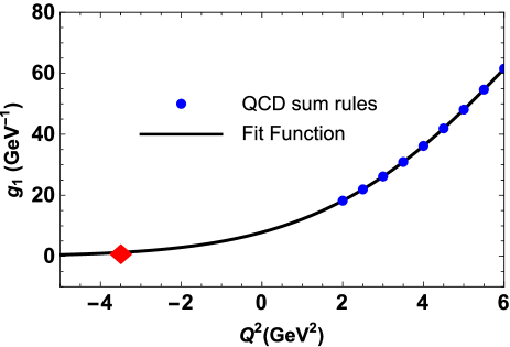
Figure 3: The sum rule predictions and fit function for the strong coupling $g_{1}(Q^{2})$. The red diamond shows the point $Q^{2}=-m_{D}^{2}$.

III.2 Process $T_{\mathrm{AV}}\rightarrow D^{\ast}(2007)^{0}D_{s}^{+}$

The second decay $T_{\mathrm{AV}}\rightarrow D^{\ast}(2007)^{0}D_{s}^{+}$ can be explored by the same manner. The correlation function which should be considered in this case is

$$\widetilde{\Pi}_{\mu\nu}(p,p^{\prime}) = i^{2}\int d^{4}xd^{4}ye^{i(p^{\prime}y-px)}\langle 0|\mathcal{T}\{J^{D_{s}}(y)$$ (46)

$$\times J_{\nu}^{D^{\ast 0}}(0)J_{\mu}^{\dagger}(x)\}|0\rangle,$$

where $\ J_{\nu}^{D^{\ast 0}}(0)$ and $J^{D_{s}}(y)$ are the interpolating currents of the mesons $D^{\ast}(2007)^{0}$ and $D_{s}^{+}$, respectively. These currents are determined by the formulas

$$J_{\nu}^{D^{\ast 0}}(x) = \overline{u}_{i}(x)\gamma_{\nu}c_{i}(x),$$

$$J^{D_{s}}(x) = \overline{s}_{j}(x)i\gamma_{5}c_{j}(x).$$ (47)

To find the physical side of the sum rule, we use recipes described above and get

$$\widetilde{\Pi}_{\mu\nu}^{\mathrm{Phys}}(p,p^{\prime})=g_{2}(q^{2})\frac{m_{D^{\ast 0}}f_{D^{\ast 0}}m_{D_{s}}^{2}f_{D_{s}}fm}{(m_{c}+m_{s})(p^{2}-m^{2})(q^{2}-m_{D^{\ast 0}}^{2})}$$

$$\times\frac{1}{(p^{\prime 2}-m_{D_{s}}^{2})}\left(\frac{m^{2}-m_{D_{s}}^{2}+q^{2}}{2}g_{\mu\nu}-q_{\mu}p_{\nu}\right)+\cdots,$$

(48)

where $m_{D^{\ast 0}}$, $m_{D_{s}}$ and $f_{D^{\ast 0}}$, $f_{D_{s}}$ are the masses and decay constants of the mesons $D^{\ast}(2007)^{0}$ and $D_{s}^{+}$, respectively.

In deriving of Eq. (48), we have used the following matrix elements:

$$\langle 0|J_{\nu}^{D^{\ast 0}}|D^{\ast 0}(q,\varepsilon^{\prime})\rangle=m_{D^{\ast 0}}f_{D^{\ast 0}}\varepsilon_{\nu}^{\prime},\$$

$$\langle 0|J^{D_{s}}|D_{s}^{+}\rangle=\frac{m_{D_{s}}^{2}f_{D_{s}}}{m_{c}+m_{s}},$$

$$\langle D^{\ast 0}(q,\varepsilon^{\prime})D_{s}^{+}(p^{\prime})|T_{\mathrm{AV}}(p,\epsilon)\rangle=g_{2}(q^{2})\left[\left(p\cdot q\right)\left(\epsilon\cdot\varepsilon^{\prime\ast}\right)\right.$$

$$\left.-\left(q\cdot\epsilon\right)\left(p\cdot\varepsilon^{\prime\ast}\right)\right].$$ (49)

Here $g_{2}$ is the strong coupling, which corresponds to the vertex $T_{\mathrm{AV}}D^{\ast}(2007)^{0}D_{s}^{+}$ and is defined at the mass shell of the $D^{\ast}(2007)^{0}$ meson,

$$g_{2}=\mathcal{F}_{2}(-m_{D^{\ast 0}}^{2}).$$ (50)

The fit function $\mathcal{F}_{2}(Q^{2})$ is given by Eq. (41) with the parameters: $\mathcal{F}_{2}^{0}=5.36~{}\mathrm{GeV}^{-1}$, $c_{2}^{1}=3.68$, and $c_{2}^{2}=-15.73$. The partial width of this decay can be calculated by means of the formula in Eq. (43) with evident replacements $g_{1}\rightarrow g_{2}$, $m_{D_{s}^{\ast}}^{2}\rightarrow m_{D^{\ast 0}}^{2}$ and $\lambda\left(m,m_{D_{s}^{\ast}},m_{D}\right)\rightarrow\lambda\left(m,m_{D^{\ast 0}},m_{D_{s}}\right)$.

In the sum rule computations, we use Eq. (25) and $M^{2}_{2}\in[2.5,3.5]~{}\mathrm{GeV}^{2}$, $s^{\prime}_{0}\in[5,7]~{}\mathrm{GeV}^{2}$. As a result, we find

$$g_{2}\equiv\mathcal{F}_{2}(-m_{D^{\ast 0}}^{2})=(7.8\pm 0.9)\cdot 10^{-1}\ \mathrm{GeV}^{-1}.$$ (51)

Then, the width of the process $T_{\mathrm{AV}}\rightarrow D^{\ast}(2007)^{0}D_{s}^{+}$ is equal to

$$\Gamma\left[T_{\mathrm{AV}}\rightarrow D^{\ast}(2007)^{0}D_{s}^{+}\right]=(19\pm 5)~{}\mathrm{MeV}.$$ (52)

For the full width of the exotic axial-vector meson $T_{\mathrm{AV}}$, we get

$$\Gamma_{\mathrm{AV}}=(72\pm 13)~{}\mathrm{MeV}.$$ (53)

Quantity	Value (in $\mathrm{MeV}$ units)
$m_{D_{s}^{\ast}}$	$2112.2\pm 0.4$
$m_{D}$	$1864.84\pm 0.05$
$m_{D_{s}}$	$1969.0\pm 1.4$
$m_{D^{\ast 0}}$	$2006.85\pm 0.05$
$f_{D_{s}^{\ast}}$	$268.8\pm 6.5$
$f_{D}$	$212.0\pm 0.7$
$f_{D_{s}}$	$249.9\pm 0.5$
$f_{D^{\ast 0}}$	$223.5\pm 8.4$

Table 1: Masses and decay constants of the mesons $D_{s}^{\ast+}$, $D^{0}$, $D_{s}^{+}$, and $D^{\ast}(2007)^{0}$, which have been used in numerical computations.

This result is rather stable prediction for $\Gamma_{\mathrm{AV}}$, because in the region $3995~{}\mathrm{MeV}\leq m\leq 4138~{}\mathrm{MeV}$ there are not other allowed decays of $T_{\mathrm{AV}}$, and its full width may undergone only small variations due to changes of $m$ and $\lambda$ in Eq. (43).

IV Full widths of $T_{\mathrm{S}}$ and $\widetilde{T}_{\mathrm{S}}$

In the case of the scalar tetraquark $T_{\mathrm{S}}$, the $S$-wave decay channels which contribute to its full width are the processes $T_{\mathrm{S}}\rightarrow D^{0}D_{s}^{+}$ and $T_{\mathrm{S}}\rightarrow D^{\ast}(2007)^{0}D_{s}^{\ast+}$. The two-meson thresholds for these decays $3833~{}\mathrm{MeV}$ and $4119~{}\mathrm{MeV}$ make them dominant channels of the tetraquark $T_{\mathrm{S}}$. There are other channels via of which the scalar four-quark state $cc\overline{u}\overline{s}$ may transform to conventional charmed mesons. For example, decays to meson pairs $D_{0}^{\ast}(2400)^{0}D_{s0}^{\ast}(2317)^{+}$ and $D^{\ast}(2007)^{0}D_{s0}^{\ast}(2317)^{+}$ are possible $S$- and $P$-wave modes of $cc\overline{u}\overline{s}$, respectively. But thresholds for production of these and other pairs exceed considerably the maximal value $m_{\mathrm{S}}=4270~{}\mathrm{MeV}$ predicted for $T_{\mathrm{S}}$. In the case of $\widetilde{T}_{\mathrm{S}}$, we explore the decay $\widetilde{T}_{\mathrm{S}}\rightarrow D^{0}D_{s}^{+}$ allowed by its mass $\widetilde{m}_{\mathrm{S}}=4035~{}\mathrm{MeV}$.

IV.1 Decay modes $T_{\mathrm{S}}\rightarrow D^{0}D_{s}^{+}$ and $T_{\mathrm{S}}\rightarrow D^{\ast}(2007)^{0}D_{s}^{\ast+}$

The treatment of the decays $T_{\mathrm{S}}\rightarrow D^{0}D_{s}^{+}$ and $T_{\mathrm{S}}\rightarrow D^{\ast}(2007)^{0}D_{s}^{\ast+}$ in the context of the three-point sum rule approach does differ from our analysis made in the previous section. Here, one should find the strong couplings $G_{1}$ and $G_{2}$ at the relevant vertices. For the coupling $G_{1}$ the correlation function of interest is

$$\Pi(p,p^{\prime})=i^{2}\int d^{4}xd^{4}ye^{i(p^{\prime}y-px)}\langle 0|\mathcal{T}\{J^{D_{s}}(y)$$

$$\times J^{D^{0}}(0)J^{\dagger}(x)\}|0\rangle,$$ (54)

where all interpolating currents have been defined above. Thus, the current $J(x)$ of the scalar tetraquark $T_{\mathrm{S}}$ has been introduced in Eq. (2), whereas $J^{D^{0}}(x)$ and $J^{D_{s}}(x)$ have been determined by Eqs. (31) and (47), respectively.

The physical side of the sum rule has the form

$$\Pi^{\mathrm{Phys}}(p,p^{\prime})=\frac{\langle 0|J^{D_{s}}|D_{s}^{+}(p^{\prime})\rangle\langle 0|J^{D^{0}}|D^{0}(q)\rangle}{(p^{\prime 2}-m_{D_{s}}^{2})(q^{2}-m_{D}^{2})}$$

$$\times\frac{\langle D^{0}(q)D_{s}^{+}(p^{\prime})|T_{\mathrm{S}}(p)\rangle\langle T_{\mathrm{S}}(p)|J^{\dagger}|0\rangle}{(p^{2}-m_{\mathrm{S}}^{2})}+\cdots.$$ (55)

The matrix elements of the mesons $D^{0}$ and $D_{s}^{+}$ have been defined by Eqs. (33) and (49), respectively. We model the matrix element $\langle D^{0}(q)D_{s}^{+}(p^{\prime})|T_{\mathrm{S}}(p)\rangle$ as

$$\langle D^{0}(q)D_{s}^{+}(p^{\prime})|T_{\mathrm{S}}(p)\rangle=G_{1}(q^{2})p\cdot p^{\prime}.$$ (56)

These matrix elements allow us to rewrite $\Pi^{\mathrm{Phys}}(p,p^{\prime})$ in a simplified form,

$$\Pi^{\mathrm{Phys}}(p,p^{\prime})=G_{1}(q^{2})\frac{m_{D}^{2}f_{D}m_{D_{s}}^{2}f_{D_{s}}f_{\mathrm{S}}m_{\mathrm{S}}}{m_{c}(m_{c}+m_{s})(p^{2}-m_{\mathrm{S}}^{2})}$$

$$\times\frac{m_{\mathrm{S}}^{2}+m_{D_{s}}^{2}-q^{2}}{2(q^{2}-m_{D}^{2})(p^{\prime 2}-m_{D_{s}}^{2})}+\cdots.$$ (57)

As is seen, the correlation function $\Pi^{\mathrm{Phys}}(p,p^{\prime})$ has a simple Lorentz structure proportional to $\mathrm{I}$, therefore we employ the whole expression in Eq. (57) as an invariant amplitude to derive the sum rule for $G_{1}(q^{2})$.

After some calculations, we find also the QCD side of the required sum rule

$$\Pi^{\mathrm{OPE}}(p,p^{\prime})=\int d^{4}xd^{4}ye^{i(p^{\prime}y-px)}$$

$$\times\left\{\mathrm{Tr}\left[\gamma_{5}S_{c}^{ja}(y-x)\gamma_{\mu}\widetilde{S}_{c}^{ib}(-x)\gamma_{5}\widetilde{S}_{u}^{ai}(x)\gamma^{\mu}\right.\right.$$

$$\left.\times S_{s}^{bj}(x-y)\right]-\mathrm{Tr}\left[\gamma_{5}S_{c}^{jb}(y-x)\gamma_{\mu}\widetilde{S}_{c}^{ia}(-x)\right.$$

$$\left.\left.\times\gamma_{5}\widetilde{S}_{u}^{ai}(x)\gamma^{\mu}S_{s}^{bj}(x-y)\right]\right\}.$$ (58)

Then the sum rule for the coupling $G_{1}(q^{2})$ reads

$$G_{1}(q^{2})=\frac{2m_{c}(m_{c}+m_{s})}{m_{D}^{2}f_{D}m_{D_{s}}^{2}f_{D_{s}}f_{\mathrm{S}}m_{\mathrm{S}}}\frac{q^{2}-m_{D}^{2}}{m_{\mathrm{S}}^{2}+m_{D_{s}}^{2}-q^{2}}$$

$$\times e^{m_{\mathrm{S}}^{2}/M_{1}^{2}}e^{m_{D_{s}}^{2}/M_{2}^{2}}\Pi_{\mathrm{scal}}(\mathbf{M}^{2},\mathbf{s}_{0},q^{2}),$$ (59)

where $\Pi_{\mathrm{scal}}(\mathbf{M}^{2},\mathbf{s}_{0},q^{2})$ is the correlation function $\Pi^{\mathrm{OPE}}(p,p^{\prime})$ after the Borel transformation and subtraction operations. It is calculated by taking into account the nonperturbative terms up to dimension $6$, as two similar functions in the previous section.

Computations carried out in accordance with a scheme described above, give the following predictions

$$G_{1}=\mathcal{F}_{3}(-m_{D}^{2})=(1.01\pm 0.21)\ \mathrm{GeV}^{-1},$$ (60)

where parameters of the function $\mathcal{F}_{3}(Q^{2})$ are: $\mathcal{F}_{3}^{0}=4.10~{}\mathrm{GeV}^{-1}$, $c_{3}^{1}=4.86$, and $c_{3}^{2}=-9.90$. It is worth nothing that the fit function is given by Eq. (41) with substitution $m\rightarrow m_{S}$. In the sum rule computations for the $T_{S}$ channel, we employ the parameters from Eq. (25).

The partial width of this decay is determined by the expression

$$\Gamma\left[T_{\mathrm{S}}\rightarrow D^{0}D_{s}^{+}\right]=\frac{G_{1}^{2}m_{D_{s}}^{2}\lambda}{8\pi}\left(1+\frac{\lambda^{2}}{m_{D_{s}}^{2}}\right),$$ (61)

with $\lambda$ being equal to $\lambda\left(m_{\mathrm{S}},m_{D_{s}},m_{D}\right)$. Numerical computations yield

$$\Gamma\left[T_{\mathrm{S}}\rightarrow D^{0}D_{s}^{+}\right]=(138\pm 41)~{}\mathrm{MeV}.$$ (62)

To determine the coupling $G_{2}$ and study the decay $T_{\mathrm{S}}\rightarrow D^{\ast}(2007)^{0}D_{s}^{\ast+}$, we analyze the correlation function

$$\widehat{\Pi}_{\mu\nu}(p,p^{\prime})=i^{2}\int d^{4}xd^{4}ye^{i(p^{\prime}y-px)}\langle 0|\mathcal{T}\{J_{\mu}^{D_{s}^{\ast}}(y)$$

$$\times J_{\nu}^{D^{\ast 0}}(0)J^{\dagger}(x)\}|0\rangle,$$ (63)

with $J_{\mu}^{D_{s}^{\ast}}(y)$ and $J_{\nu}^{D^{\ast 0}}(0)$ being the interpolating currents of the vector mesons $D_{s}^{\ast+}$ and $D^{\ast}(2007)^{0}$ given by Eqs. (31) and (47), respectively.

The function $\widehat{\Pi}_{\mu\nu}(p,p^{\prime})$ in terms of the physical parameters of the tetraquark $T_{\mathrm{S}}$ and mesons $D_{s}^{\ast+}$ and $D^{\ast}(2007)^{0}$ is equal to expression

$$\widehat{\Pi}_{\mu\nu}^{\mathrm{Phys}}(p,p^{\prime})=G_{2}(q^{2})\frac{m_{D_{s}^{\ast}}f_{D_{s}^{\ast}}m_{D^{\ast 0}}f_{D^{\ast 0}}f_{\mathrm{S}}m_{\mathrm{S}}}{(p^{2}-m_{\mathrm{S}}^{2})(p^{\prime 2}-m_{D_{s}^{\ast}}^{2})}$$

$$\times\frac{1}{(q^{2}-m_{D^{\ast 0}}^{2})}\left(\frac{m_{\mathrm{S}}^{2}-m_{D_{s}^{\ast}}^{2}-q^{2}}{2}g_{\mu\nu}-q_{\mu}p_{\nu}^{\prime}\right)+\cdots,$$

where the vertex $\langle D^{\ast}(2007)^{0}(q,\varepsilon)D_{s}^{\ast+}(p^{\prime},\varepsilon^{\prime})|T_{\mathrm{S}}(p)\rangle$ is modeled in the form

$$\langle D^{\ast}(2007)^{0}(q,\varepsilon)D_{s}^{\ast+}(p^{\prime},\varepsilon^{\prime})|T_{\mathrm{S}}(p)\rangle=G_{2}(q^{2})$$

$$\times\left[\left(p^{\prime}\cdot q\right)\left(\varepsilon^{\ast}\cdot\varepsilon^{\prime\ast}\right)-\left(q\cdot\varepsilon^{\prime\ast}\right)\left(p^{\prime}\cdot\varepsilon^{\ast}\right)\right].$$ (65)

In terms of the quark-gluon degrees of freedom, $\widehat{\Pi}_{\mu\nu}^{\mathrm{OPE}}(p,p^{\prime})$ is given by the formula

$$\widehat{\Pi}_{\mu\nu}^{\mathrm{OPE}}(p,p^{\prime})=\int d^{4}xd^{4}ye^{i(p^{\prime}y-px)}\left\{\mathrm{Tr}\left[\gamma_{\mu}S_{c}^{ia}(y-x)\right.\right.$$

$$\left.\times\gamma_{\alpha}\widetilde{S}_{c}^{jb}(-x)\gamma_{\nu}\widetilde{S}_{s}^{bj}(x)\gamma^{\alpha}S_{u}^{ai}(x-y)\right]$$

$$\left.-\mathrm{Tr}\left[\gamma_{\mu}S_{c}^{ib}(y-x)\gamma_{\alpha}\widetilde{S}_{c}^{ja}(-x)\gamma_{\nu}\widetilde{S}_{s}^{bj}(x)\gamma^{\alpha}S_{u}^{ai}(x-y)\right]\right\}.$$

(66)

Omitting details of rather standard computations, let us write down the final results:

$$G_{2}=\mathcal{F}_{4}(-m_{D^{\ast 0}}^{2})=(2.11\pm 0.43)\ \mathrm{GeV}^{-1},$$ (67)

where parameters of the function $\mathcal{F}_{4}(Q^{2})$ are: $\mathcal{F}_{4}^{0}=3.17~{}\mathrm{GeV}^{-1}$, $c_{4}^{1}=1.14$, and $c_{4}^{2}=-2.51$.

The partial width of this decay is equal to

$$\Gamma\left[T_{\mathrm{S}}\rightarrow D^{\ast}(2007)^{0}D_{s}^{\ast+}\right]=(75\pm 22)~{}\mathrm{MeV}.$$ (68)

Using Eqs. (62) and (68), we find

$$\Gamma_{\mathrm{S}}=(213\pm 47)~{}\mathrm{MeV}.$$ (69)

IV.2 Decay $\widetilde{T}_{\mathrm{S}}\rightarrow D^{0}D_{s}^{+}$

For the decay $\widetilde{T}_{\mathrm{S}}\rightarrow D^{0}D_{s}^{+}$ one should employ the following correlation function

$$\widetilde{\Pi}^{\mathrm{OPE}}(p,p^{\prime})=-\int d^{4}xd^{4}ye^{i(p^{\prime}y-px)}$$

$$\times\left\{\mathrm{Tr}\left[\gamma_{5}S_{c}^{ja}(y-x)\gamma_{5}\widetilde{S}_{c}^{ib}(-x)\gamma_{5}\widetilde{S}_{u}^{ai}(x)\gamma_{5}\right.\right.$$

$$\left.\times S_{s}^{bj}(x-y)\right]+\mathrm{Tr}\left[\gamma_{5}S_{c}^{jb}(y-x)\gamma_{5}\widetilde{S}_{c}^{ia}(-x)\right.$$

$$\left.\left.\times\gamma_{5}\widetilde{S}_{u}^{ai}(x)\gamma_{5}S_{s}^{bj}(x-y)\right]\right\}.$$ (70)

Then $\widetilde{G}(q^{2})$ can be extracted from the sum rule

$$\widetilde{G}(q^{2})=\frac{2m_{c}(m_{c}+m_{s})}{m_{D}^{2}f_{D}m_{D_{s}}^{2}f_{D_{s}}\widetilde{f}_{\mathrm{S}}\widetilde{m}_{\mathrm{S}}}\frac{q^{2}-m_{D}^{2}}{\widetilde{m}_{\mathrm{S}}^{2}+m_{D_{s}}^{2}-q^{2}}$$

$$\times e^{\widetilde{m}_{\mathrm{S}}^{2}/M_{1}^{2}}e^{m_{D_{s}}^{2}/M_{2}^{2}}\widetilde{\Pi}_{\mathrm{scal}}(\mathbf{M}^{2},\mathbf{s}_{0},q^{2}),$$ (71)

where $\widetilde{\Pi}_{\mathrm{scal}}(\mathbf{M}^{2},\mathbf{s}_{0},q^{2})$ is the Borel transformed and subtracted correlation function $\widetilde{\Pi}^{\mathrm{OPE}}(p,p^{\prime})$.

Computations give the following predictions:

$$\widetilde{G}=\mathcal{F}_{5}(-m_{D}^{2})=(1.07\pm 0.21)\ \mathrm{GeV}^{-1},$$ (72)

where parameters of the function $\mathcal{F}_{5}(Q^{2})$, obtained from Eq. (41) after the replacement $m\rightarrow\tilde{m}_{S}$, are: $\mathcal{F}_{5}^{0}=4.06~{}\mathrm{GeV}^{-1}$, $c_{5}^{1}=4.56$, and $c_{5}^{2}=-7.82$.

The partial width of this decay is determined by the expression Eq. (61) after substitutions $G_{1}\rightarrow\widetilde{G}$, $m_{\mathrm{S}}\rightarrow$ $\widetilde{m}_{\mathrm{S}}$ and $\lambda\rightarrow$ $\widetilde{\lambda}=$ $\lambda(\widetilde{m}_{\mathrm{S}},m_{D_{s}},m_{D})$.

Numerical computations yield

$$\widetilde{\Gamma}_{\mathrm{S}}=(123\pm 32)~{}\mathrm{MeV},$$ (73)

which characterizes $\widetilde{T}_{\mathrm{S}}$ as a wide resonance.

V Discussion and concluding notes

The main motivation for present investigation is the LHCb discovery of the very narrow doubly charmed axial-vector state $T_{cc}^{+}$. It is special in two respects: First, $T_{cc}^{+}$ is the only doubly charmed resonance observed experimentally. Secondly, it is narrowest candidate to a four-quark meson. These circumstances made $T_{cc}^{+}$ an object of intensive theoretical studies: Its structure and parameters were investigated in numerous publications using various methods and models.

This discovery generated interest to possible counterparts of $T_{cc}^{+}$, which may be four-quark systems with the same content but different spin-parities. The doubly charmed tetraquarks containing strange $s$-quark(s) are another class of particles closely related to $T_{cc}^{+}$. In present article, we have concentrated namely on these particles and explored the axial-vector and scalar doubly charmed strange tetraquarks $T_{\mathrm{AV}}$, $T_{\mathrm{S}}$, and $\widetilde{T}_{\mathrm{S}}$ by calculating their masses and widths.

It is worth to compare predictions obtained for the mass $m=(3995\pm 143)~{}\mathrm{MeV}$ and width $\Gamma_{\mathrm{AV}}=(72\pm 13)~{}\mathrm{MeV}$ of $T_{\mathrm{AV}}$ with parameters of $T_{cc}^{+}$ measured by the LHCb Collaboration. The mass gap between these two states, in accordance with our findings, amounts to $120~{}\mathrm{MeV}$, which can be considered as a reasonable estimate for particles with a $s$-quark difference in their contents. The two-meson states $D^{0}D_{s}^{\ast+}$ and $D^{\ast}(2007)^{0}D_{s}^{+}$ play for the tetraquark $T_{\mathrm{AV}}$ the same role as $D^{0}D^{\ast}{}^{+}$ for the resonance $T_{cc}^{+}$. The mass of $T_{cc}^{+}$ is very close but less than $D^{0}D^{\ast}{}^{+}$ threshold, whereas $T_{\mathrm{AV}}$ lies $\approx 20~{}\mathrm{MeV}$ above corresponding thresholds, which makes its decays to mesons $D^{0}D_{s}^{\ast+}$ and $D^{\ast}(2007)^{0}D_{s}^{+}$ kinematically allowed processes. These $S$-wave channels form width of the tetraquark $T_{\mathrm{AV}}$, and our prediction for $\Gamma_{\mathrm{AV}}$ means that it is relatively wide resonance. In this aspect, $T_{\mathrm{AV}}$ differs from the very narrow state $T_{cc}^{+}$, because $T_{\mathrm{AV}}$ and $T_{cc}^{+}$ decay to ordinary mesons through different mechanisms. Thus, the decay mode $T_{cc}^{+}\rightarrow D^{0}D^{0}\pi^{+}$ in which $T_{cc}^{+}$ was discovered, may run due to the transformation $T_{cc}^{+}\rightarrow D^{0}D^{\ast+}$. But this process is forbidden, therefore the final state $D^{0}D^{0}\pi^{+}$ appears through production of intermediate scalar tetraquarks, partial widths of which are very small.

Another interesting question to be addressed here is the mass splitting between the axial-vector $T_{\mathrm{AV}}$ and scalar $T_{\mathrm{S}}$ tetraquarks. The $T_{\mathrm{AV}}$ contains $J^{\mathrm{P}}=0^{+}$ ”good” $(\mathbf{3}_{f},\mathbf{3}_{c})$ antidiquark $\overline{u}\overline{s}$, whereas $T_{\mathrm{S}}$ is made of $J^{\mathrm{P}}=1^{+}$ ”bad” $(\overline{\mathbf{6}}_{f},\mathbf{3}_{c})$ one. For the nonstrange diquark the ”bad”-”good” mass difference $\delta(1^{+}-0^{+})_{ud}$ was found from the QCD lattice calculations equal to $198~{}\mathrm{MeV}$ Francis:2021vrr , which transforms to $\delta(1^{+}-0^{+})_{us}=135~{}\mathrm{MeV}$ in the case of $\overline{u}\overline{s}$ diquark Karliner:2021wju . Then, in accordance with this scheme, $m_{\mathrm{S}}$ should be equal approximately to $4130~{}\mathrm{MeV}$. As is seen, our sum rule prediction for $m_{\mathrm{S}}=(4128\pm 142)~{}\mathrm{MeV}$ agrees well with this estimate. The tetraquark $\widetilde{T}_{\mathrm{S}}$ built of color-sextet scalar diquarks resides between $T_{\mathrm{AV}}$ and $T_{\mathrm{S}}$ states. In a situation when an existence of a scalar state $cc\overline{u}\overline{s}$ with ”good” components is forbidden, the axial-vector tetraquark $T_{\mathrm{AV}}$ becomes the lightest particle in the spectrum.

The four-quark structure $cc\overline{u}\overline{s}$ with $J^{\mathrm{P}}=1^{+}$ was studied in other publications in the framework of alternative approaches. In the diquark-antidiquark and molecule models its mass was estimated as $4106~{}\mathrm{MeV}$ and $3974.8_{-0.5}^{+0.4}~{}\mathrm{MeV}$ in Refs. Karliner:2021wju and Ren:2021dsi , respectively. As it has been emphasized above, the prediction around of $3975~{}\mathrm{MeV}$ contradicts to experimental-theoretical constraints on the mass of $T_{\mathrm{AV}}$. Our result is less than the prediction made in Ref. Karliner:2021wju though $m$ in upper limit overlaps with it.

One sees, that there are interesting open problems in physics of doubly charmed four-quark mesons, which require additional theoretical and experimental studies. The information gained in this article on the masses and widths of the strange doubly-charmed tetraquarks gives new perspectives on these states and can be used in future experimental investigations of multiquark hadrons.

Data Availability Statement: No Data associated in the manuscript.

References

- (1) R. Aaij et al. [LHCb Collaboration], Nature Phys. 18, 751 (2022).
- (2) R. Aaij et al. [LHCb Collaboration], Nature Commun. 13, 1 (2022).
- (3) A. Esposito, M. Papinutto, A. Pilloni, A. D. Polosa, and N. Tantalo, Phys. Rev. D 88, 054029 (2013).
- (4) F. S. Navarra, M. Nielsen, and S. H. Lee, Phys. Lett. B 649, 166 (2007).
- (5) M. Karliner and J. L. Rosner, Phys. Rev. Lett. 119, 202001 (2017).
- (6) E. J. Eichten and C. Quigg, Phys. Rev. Lett. 119, 202002 (2017).
- (7) S. S. Agaev, K. Azizi, B. Barsbay and H. Sundu, Phys. Rev. D 99, 033002 (2019).
- (8) S. S. Agaev, K. Azizi, B. Barsbay, and H. Sundu, Eur. Phys. J. A 57, 106 (2021).
- (9) Y. Xing and R. Zhu, Phys. Rev. D 98, 053005 (2018).
- (10) S. S. Agaev, K. Azizi, B. Barsbay, and H. Sundu, Chin. Phys. C 45, 013105 (2021).
- (11) S. S. Agaev, K. Azizi, B. Barsbay, and H. Sundu, Eur. Phys. J. A 56, 177 (2020).
- (12) S. S. Agaev, K. Azizi, B. Barsbay, and H. Sundu, Phys. Rev. D 101, 094026 (2020).
- (13) M. L. Du, W. Chen, X. L. Chen, and S. L. Zhu, Phys. Rev. D 87, 014003 (2013).
- (14) Z. G. Wang, Acta Phys. Polon. B 49, 1781 (2018).
- (15) Z. G. Wang and Z. H. Yan, Eur. Phys. J. C 78, 19 (2018).
- (16) E. Braaten, L. P. He, and A. Mohapatra, Phys. Rev. D 103, 016001 (2021).
- (17) J. B. Cheng, S. Y. Li, Y. R. Liu, Z. G. Si, and T. Yao, Chin. Phys. C 45, 043102 (2021).
- (18) Q. Meng, E. Hiyama, A. Hosaka, M. Oka, P. Gubler, K. U. Can, T. T. Takahashi, and H. S. Zong, Phys. Lett. B 814, 136095 (2021).
- (19) P. Junnarkar, N. Mathur, and M. Padmanath, Phys. Rev. D 99, 034507 (2019).
- (20) T. Guo, J. Li, J. Zhao, and L. He, Phys. Rev. D 105, 014021 (2022).
- (21) M. Padmanath, and S. Prelovsek, Phys. Rev. Lett. 129, 032002 (2022).
- (22) S. S. Agaev, K. Azizi, and H. Sundu, Phys. Rev. D 99, 114016 (2019).
- (23) S. S. Agaev, K. Azizi, B. Barsbay, and H. Sundu, Nucl. Phys. B 939, 130 (2019).
- (24) A. Feijoo, W. H. Liang, and E. Oset, Phys. Rev. D 104, 114015 (2021).
- (25) M. J. Yan and M. P. Valderrama, Phys. Rev. D 105, 014007 (2022).
- (26) S. Fleming, R. Hodges, and T. Mehen, Phys. Rev. D 104, 116010 (2021).
- (27) S. S. Agaev, K. Azizi, and H. Sundu, Nucl. Phys. B 975, 115650 (2022).
- (28) S. S. Agaev, K. Azizi, and H. Sundu, JHEP 06, 057 (2022).
- (29) M. Karliner and J. L. Rosner, Phys. Rev. D 105, 034020 (2022).
- (30) X. Chen, F. L. Wang, Y. Tan and Y. Yang arXiv:2206.10917 [hep-ph].
- (31) M. Praszalowicz, Phys. Rev. D 106, 114005 (2022).
- (32) Q. Xin and Z. G. Wang Eur. Phys. J. A 58, 110 (2022).
- (33) H. Ren, F. G. Wu, and R. Zhu Adv. High Energy Phys. 2022, 9103031 (2022).
- (34) M. A. Shifman, A. I. Vainshtein, and V. I. Zakharov, Nucl. Phys. B 147, 385 (1979).
- (35) M. A. Shifman, A. I. Vainshtein and V. I. Zakharov, Nucl. Phys. B 147, 448 (1979).
- (36) S. S. Agaev, K. Azizi and H. Sundu, Turk. J. Phys. 44, 95 (2020).
- (37) C. J. Burden, L. Qian, C. D. Roberts, P. C. Tandy, and M. J. Thomson, Phys. Rev. C 55, 2649 (1997).
- (38) R. L. Workman et al. [Particle Data Group], Prog. Theor. Exp. Phys. 2022, 083C01 (2022).
- (39) V. Lubicz, A. Melis and S. Simula, PoS LATTICE 2016, 291 (2017).
- (40) A. Francis, P. de Forcrand, R. Lewis, and K. Maltman, JHEP 05, 062 (2022).