Quantum-to-classical crossover in single-electron emitter

Abstract

We investigate the temperature-driven quantum-to-classical crossover in a single-electron emitter. The emitter is composed of a quantum conductor and an electrode, which is coupled via an Ohmic contact. At zero temperature, it has been shown that a single electron can be injected coherently by applying an unit-charge Lorentzian pulse on the electrode. As the electrode temperature increases, we show that the electron emission approaches a time-dependence Poisson process at long times. The Poissonian character is demonstrated from the time-resolved full counting statistics. In the meantime, we show that the emission events remain correlated, which is due to the Pauli exclusion principle. The correlation is revealed from the emission rates of individual electrons, from which a characteristic correlation time can be extracted. The correlation time drops rapidly as the electrode temperature increases, indicating that correlation can only play a non-negligible role at short times in the high-temperature limit. By using the same procedure, we further show that the quantum-to-classical crossover exhibits similar features when the emission is driven by a Lorentzian pulse carrying two electron charge. Our results show how the electron emission process is affected by thermal fluctuations in a single-electron emitter.

I Introduction

The on-demand control of coherent electron emission in mesoscopic conductors has attracted much interest in recent decades [1, 2]. In a simple setup, the electrons are emitted from an electrode into a conductor though an Ohmic contact, which are driven by voltage pulses $V(t)$. For a single-channel quantum conductor, the current $I(t)$ follows instantly to $V(t)$ as $I(t)=e^{2}V(t)/h$, with $e$ being the electron charge and $h$ being the Planck constant. However, the details of the emission process can be quite different in quantum and classical limits.

In the quantum limit, the current is due to the coherent emission of electrons or holes, which are usually accompanied by neutral electron-hole pairs. Their wave functions are well-defined, which can be extracted by quantum tomography methods [3, 4, 5, 6, 7]. In particular, by using an unit-charge Lorentzian pulse $V(t)$ with time width $W$, i.e., $V(t)=hW/[\pi e(W^{2}+t^{2})]$, a single electron can be emitted on top of the Fermi sea without accompanied electron-hole pairs [8, 9]. It has been called a leviton, whose wave function can be given as $\psi_{L}(t)=\sqrt{W/(2\pi)}/(t+iW/2)$. The emission probability density of the leviton follows instantly to the voltage pulse as $\left|\psi_{L}(t)\right|^{2}=I(t)/e=eV(t)/h$, indicating an excellent synchronization between the electron emission and driving voltage. In contrast, the current corresponds to the incoherent emission of electrons and/or holes in the classical limit. This typically occurs at high temperatures, when thermal fluctuations in the electrode can play an important role. The emission events can be treated as random and independent, which follow Poisson statistics. In this limit, the voltage pulse does not control the emission probability density of individual electrons. Instead, it decides the overall emission rate of the emission process.

One expects that the quantum to classical crossover occurs as the temperature of the electrode increases. Indeed, the many-body quantum state of the emitted electrons can evolve from a pure state into a mixed one due to thermal fluctuations [10, 11]. This can lead to a reduction of the dc shot noise [12, 13, 14]. But the electron anti-bunching is robust against temperature, which has been revealed from the Hong-Ou-Mandel interference [12]. This indicates that the quantum coherence between different electrons is still preserved and hence the temperature-induced quantum-to-classical crossover is incomplete. In the case of dc driving when $V(t)=V_{0}$, this has been clearly demonstrated from the waiting time distribution $\mathcal{W}(\tau)$ (WTD), which gives the distribution of time delays $\tau$ between successive electrons [15, 16, 17, 18, 19]. At zero temperature, $\mathcal{W}(\tau)$ follows the Wigner-Dyson distribution, which has a zero dip around $\tau=0$ and a Gaussian tail as $\tau\to+\infty$ [16]. As the electrode temperature $T$ increases, the tail approaches an exponential distribution when $T$ is comparable to $eV_{0}/k_{B}$, with $k_{B}$ being the Boltzmann constant. In contrast, the essential shape of $\mathcal{W}(\tau)$ remains unchanged, especially around the zero dip [17]. This implies that the emission approaches a Poisson process at long times, but the emission events are still correlated at short times.

However, the crossover can have a different nature when the emission is driving by the Lorentzian pulse. First, the pulse width $W$ provides an important time scale in this case. In fact, it decides the crossover temperature, which separates the high- and low-temperature regions for the dc shot noise [10]. Secondly, the full counting statistics (FCS) changes drastically as the temperature increases: In the classical limit, the emission tends to follow the Poisson statistics. While in the quantum limit, the voltage pulse injects exactly one electron into the quantum conductor. This make the WTD less suitable for the study of emission in this limit. Finally, as the emission is triggered by a time-dependent voltage, it is helpful to elucidate the relation between the electron emission and the driving voltage, which is also absent from the WTD.

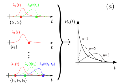
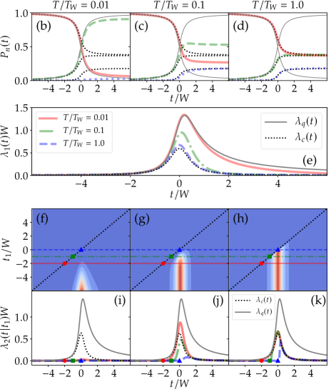
Figure 1: (a) Illustration for the real-time electron counting measurements. A single measurement is represented by a sequence of random points in the time trace. The $k$-th point in each time trace represents the emission time of the $k$-th electron. The emission of the $k$-th electron is governed by the corresponding emission rate $\lambda_{k}(t|t_{1},\dots,t_{k-1})$. In the figure, we mark the emission of the first, second and third electrons by the red, green and blue dots, which correspond to the emission rate $\lambda_{1}(t)$, $\lambda_{2}(t|t_{1})$ and $\lambda_{3}(t|t_{1},t_{2})$, respectively. The time-resolved FCS $P_{n}(t)$ is obtained from the statistics gathered from a large number of measurements. (b-d) The time-resolved FCS $P_{n}(t)$ at different temperatures $T/T_{W}=0.01$ (b), $T/T_{W}=0.1$ (c) and $T/T_{W}=1.0$ (d). The red solid, green dashed and blue dotted curves correspond to $n=0$, $1$ and $2$, respectively. The thin gray solid curves correspond to the quantum limit from Eq. (1). The thin black dotted curves represent the classical limit from Eq. (2). (e) The emission rate $\lambda_{1}(t)$ of the first electron at different temperatures. The gray solid and black dotted curves represent the quantum and classical limit for the emission rate. See text for details. (f-h) The emission rate $\lambda_{2}(t|t_{1})$ of the second electron at different temperatures $T/T_{W}=0.01$ (f), $T/T_{W}=0.1$ (g) and $T/T_{W}=1.0$ (h). They are shown as contour plots in the $t$-$t_{1}$ plane. (i-j) The emission rate $\lambda_{2}(t|t_{1})$ as a function of $t$ for three typical $t_{1}$ at different temperatures. The red solid, green dash-dotted and blue dashed curves correspond to $t_{1}/W=-2.0$, $-1.0$ and $0.0$, while the red dots, green squares and blue triangles represent the point $t=t_{1}$, respectively. The classical and quantum limit of the emission rates $\lambda_{q}(t)$ and $\lambda_{c}(t)$ are also plotted by the gray solid and black dotted curves for comparison.

To solve this problem, in this paper we discuss the quantum-to-classical crossover by combining the time-resolved full counting statistics and electron emission rates. The time-resolved FCS $P_{n}(t)$ gives the probability of emitting $n$ electrons up to a given time $t$, which can be extracted from the statistics gathered on a large number of measurements [37]. Each single measurement is represented by a random time sequence $\{t_{1},t_{2},\dots,t_{k},\dots t_{n}\}$, where each $t_{k}$ stands for the emission time of the $k$-th electron [See Fig. 1(a) for illustration]. The emission of the $k$-th electron is governed by the corresponding emission rate $\lambda_{k}(t|t_{1},t_{2},\dots,t_{k-1})$, which describes the expected number of electrons emitted in a given infinitesimal time interval $[t,t+dt]$. As the emission events are generally correlated in quantum conductors [20], the emission rate depends not only on the time $t$, but also on the emission times $\{t_{1},t_{2},\dots,t_{k-1}\}$ of all previously emitted electrons.

The typical temperature-dependence of $P_{n}(t)$ is illustrated in Fig. 1(b-d). In the quantum limit when the temperature $T$ is very low, $P_{n}(t)$ can be well-approximated from the wave function of leviton as

$$P_{n}(t) = \begin{cases}1-\int^{t}_{-\infty}d\tau\left|\psi_{L}(t)\right|^{2},&n=0\\ \int^{t}_{-\infty}d\tau\left|\psi_{L}(t)\right|^{2},&n=1\\ 0,&n\geq 2\end{cases}.$$ (1)

The quantum limit of $P_{n}(t)$ is shown by the gray solid curves in the figure. At high temperatures, $P_{n}(t)$ tends to follow the classical limit, which corresponds to the time-dependent Poisson distribution

$$P_{n}(t)=\frac{\left[\int^{t}_{-\infty}d\tau\lambda_{c}(\tau)\right]^{n}}{n!}\exp{\left[-\int^{t}_{-\infty}d\tau\lambda_{c}(\tau)\right]},$$ (2)

where the emission rate $\lambda_{c}(t)$ is decided by the driving pulse as $\lambda_{c}(t)=eV(t)/h$. The classical limit of $P_{n}(t)$ is plotted by the black dotted curves. The figure shows that $P_{n}(t)$ evolves from the quantum limit to the classical limit as the temperatures $T$ approaches $T_{W}=\hbar/(k_{B}W)$, which providing a clear signature of the quantum-to-classical crossover.

The behavior of $P_{n}(t)$ suggests that the emission rates of all the electrons should approach the classical limit $\lambda_{c}(t)$ at high temperatures. We find that this only holds for the emission rate of the first electron $\lambda_{1}(t)$, which is illustrated in Fig. 1(e). The figure shows that $\lambda_{1}(t)$ evolves from the quantum limit $\lambda_{q}(t)=V(t)/[1-\int^{t}_{-\infty}d\tau V(\tau)]$ (gray solid curve) to the classical limit $\lambda_{c}(t)$ (black dotted curve) as the temperature $T$ approaches $T_{W}$. However, other emission rates do not fully follow this behavior. This can be seen from the emission rate of the second electron $\lambda_{2}(t|t_{1})$, which are displayed as contour plots in the $t$-$t_{1}$ plane [Fig. 1(f-h)]. As the emission of the second electron is the coeffect of the driving pulse and thermal fluctuations, it remains rather small at low temperatures [Fig. 1(f)]. At moderate temperatures [Fig. 1(g)], it depends significantly on both $t$ and $t_{1}$, indicating strong correlations between the emission of the first and second electrons. In particular, $\lambda_{2}(t|t_{1})$ always drops to zero as $t$ approaches $t_{1}$. This is better demonstrated in Fig. 1(j), where the points $t=t_{1}$ for three typical $t_{1}$ are marked by the red dots, blue triangles and green squares. This indicates that the emission of the second electron is coupled to the first one due to the Pauli exclusion principle. At high temperatures [Fig. 1(h)], the correlations remain pronounced, but can only be seen at short times. We find that $\lambda_{2}(t|t_{1})$ tends to follow $\Theta(t-t_{1})\lambda_{c}(t)$ in the high temperature limit. This can be better seen from Fig. 1(k), where $\lambda_{c}(t)$ is plotted by the black dotted curve for comparison. These behaviors show that, as the electrode temperature increases, the electron emission approaches a time-dependent Poisson process at long times, but the correlations between the emission events are always preserved at short times. By using a similar procedure, we find that similar behaviors can also be seen when the emission is driven by a Lorentzian pulse carrying two electron charge.

This paper is organized as follows. In Sec. II, we introduce a procedure to calculate the time-resolved statistics and emission rates for the electron emission in quantum conductors. In Sec. III, we demonstrate the procedure by studying the single and two electron emissions at zero temperature. The finite temperature effect is discussed in Sec. IV. We summarize our results in Sec. V.

II Time-resolved statistics of a quantum emitter

The statistics of the electron emission process can be described by two equivalently ways. On one hand, it can be characterized by $n$-fold delayed coincidences, which gives the joint probability that one electron is emitted in each infinitesimal time interval $[t_{i},t_{i}+dt]$ (with $i=1,2,\dots,n$). It can be expressed as

$$g_{n}(t_{1},\dots,t_{n}) = \langle a^{\dagger}(t_{1})\dots a^{\dagger}(t_{n})a(t_{n})\dots a(t_{1})\rangle$$ (3)

$$- \langle a^{\dagger}(t_{1})\dots a^{\dagger}(t_{n})a(t_{n})\dots a(t_{1})\rangle_{0},$$

where $a^{\dagger}(t)$ and $a(t)$ represent the creation and annihilation operations of electrons, respectively. Here the two angular brackets $\langle\dots\rangle$ and $\langle\dots\rangle_{0}$ denote the quantum-statistical average over the many-body electron states with and without the emitted electrons, respectively. In doing so, one excludes the contribution from the undisturbed Fermi sea [21, 4]. The coincidences functions are just the diagonal part of the Glauber’s correlation functions [22, 23, 24, 25, 26, 27], which can be extracted from the current correlation measurements [3, 28, 4].

In contrast, the emission process can also be investigated by real-time electron counting techniques [29, 30, 31, 32, 33]. This can be used to extract the information of electron process in single-shot experiments. In this case, the emission process can be described by recording each individual emission event in a time trace [See Fig.1(a) for illustration]. This allows us to represent emission events by random points in a line. One usually further assumes that two emission events cannot occur exactly at the same time, i.e., there can only exist at most one emission event in an arbitrary infinitesimal time interval $[t,t+dt]$. This assumption has been proved to be valid for typical emission processes, such as photon emission in quantum optics and neuronal spike emission in neuroscience [24, 34, 35, 36].

The emission process can be characterized by the time-resolved statistics of these events. For example, it can be characterized by the time-dependent counting statistics $P_{n}(t_{s},t_{e})$, which gives the probability to emit $n$ electrons in a given time interval $[t_{s},t_{e}]$. It can also be described by statistics of times, such as idle time distribution $\Pi_{0}(t_{s},t_{e})$, which gives the probability that no electron is emitted in the time interval $[t_{s},t_{e}]$. The WTD can be obtained from $\Pi_{0}(t_{s},t_{e})$ by its second derivative [16]. Note that all these quantities usually depend on two times $t_{s}$ and $t_{e}$, which can be treated as the starting and ending times of the electron counting measurements.

It is inconvenient to describe the time-resolved statistics directly in terms of the $n$-fold delayed coincidences $g_{n}(t_{1},\dots,t_{n})$. In contrast, the exclusive joint probability density $f_{n}(t_{1},\dots,t_{n};t_{s},t_{e})$ (with $n\geq 1$) has been introduced [24, 38]. It gives the joint probability that one electron is emitted in each infinitesimal time interval $[t_{i},t_{i}+dt]$ (with $i=1,2,\dots,n$ and all $t_{i}\in[t_{s},t_{e}]$), while no other electron is emitted in the time interval $[t_{s},t_{e}]$. It has been shown that $f_{n}(t_{1},\dots,t_{k};t_{s},t_{e})$ can be related to $g_{n}(t_{1},\dots,t_{n})$ as

$$f_{n}(t_{1},\dots,t_{n};t_{s},t_{e})=\sum_{k=n}^{+\infty}\frac{(-1)^{k-n}}{(k-n)!}\int^{t_{e}}_{t_{s}}dt_{n+1}...\int^{t_{e}}_{t_{s}}dt_{k}g_{k}(t_{1},\dots,t_{n},t_{n+1},\dots,t_{k}).$$ (4)

This relation is derived from the definition of $f_{n}(t_{1},\dots,t_{n};t_{s},t_{e})$ and $g_{n}(t_{1},\dots,t_{n})$, which is independent on the nature of the emitted particles [24]. So it can be applied to both Bosons and Fermions.

All the time-resolved statistics can be obtained from $f_{n}(t_{1},\dots,t_{n};t_{s},t_{e})$ in a direct way. In particular, the FCS $P_{n}(t_{s},t_{e})$ for $n\geq 1$ can be given as

$$P_{n}(t_{s},t_{e})=\frac{1}{n!}\int^{t_{e}}_{t_{s}}dt_{1}\dots\int^{t_{e}}_{t_{s}}dt_{n}f_{n}(t_{1},t_{2},\dots,t_{n};t_{s},t_{e}).$$ (5)

For $n=0$, the corresponding FCS $P_{0}(t_{s},t_{e})$, or equivalently the idle time distribution $\Pi_{0}(t_{s},t_{e})$, can be obtained via the normalization relation

$$\Pi_{0}(t_{s},t_{e})=P_{0}(t_{s},t_{e})=1-\sum^{+\infty}_{n=1}P_{n}(t_{s},t_{e}).$$ (6)

Comparing to the FCS, the exclusive joint probability densities $f_{n}(t_{1},\dots,t_{n};t_{s},t_{e})$ contain much detailed information on the emission process. In particular, one can extract the emission rate of each individual electron from them [39, 36, 38]. This can be better understood by starting from a stationary Poisson process with emission rate $\lambda_{0}$. In this case, the emission events are random and independent. The corresponding coincidence function can be simply given as $g_{k}(t_{1},\dots,t_{n})=\lambda^{n}_{0}$. From Eq. (4), one finds that

$$f_{n}(t_{1},\dots,t_{n};t_{s},t_{e})=\lambda^{n}_{0}\exp[-\lambda_{0}(t_{e}-t_{s})],$$ (7)

whose FCS follows the well-known Poisson statistics

$$P_{n}(t_{s},t_{e})=\frac{\left[\lambda_{0}(t_{e}-t_{s})\right]^{n}}{n!}\exp[-\lambda_{0}(t_{e}-t_{s})].$$ (8)

The corresponding idle time distribution can be expressed as $\Pi_{0}(t_{s},t_{e})=\exp[-\lambda_{0}(t_{e}-t_{s})]$.

The physical meaning of Eq. (7) can be better seen by rewriting it in the form

$$f_{n}(t_{1},\dots,t_{n};t_{s},t_{e}) = \exp[-\lambda_{0}(t_{1}-t_{s})]$$ (9)

$$\times\prod^{n-1}_{i=1}\left\{\lambda_{0}\exp[-\lambda_{0}(t_{i+1}-t_{i})]\right\}$$

$$\times\lambda_{0}\exp[-\lambda_{0}(t_{e}-t_{n})].$$

Here each $\lambda_{0}$ gives the emission probability of an electron in each infinitesimal time interval $[t_{i},t_{i}+dt]$. The exponential factors are just idle time distributions, they ensure that no other electron can be emitted between these infinitesimal time intervals. From the above expression, one finds that the emission rate can be obtained from $f_{n}(t_{1},\dots,t_{n};t_{s},t_{e})$ as

$$\lambda_{0}=\frac{f_{n+1}(t_{1},\dots,t_{n},t_{n+1};t_{s},t_{n+1})}{f_{n}(t_{1},\dots,t_{n};t_{s},t_{n})}.$$ (10)

Alternatively, it can also be related to the idle time distribution as

$$\lambda_{0}=\frac{f_{1}(t_{1};t_{s},t_{1})}{\Pi_{0}(t_{s},t_{1})}.$$ (11)

In general cases, the emission rate of an electron has a more complicated form. On one hand, it depends explicitly on the time $t$, which is due to the time-dependence of the driving voltage. On the other hand, it also depends on the history of the emission process, which can be induced by the quantum coherence between electrons [20]. So the emission rates are different for different electrons. For the $n$-th electron, the corresponding emission rate can be written as $\lambda_{n}(t|t_{s},t_{1},\dots,t_{n-1})$. It is essentially a conditional intensity, which gives the expected number of electrons emitted in the infinitesimal time interval $[t,t+dt]$, under the condition that there are $n-1$ electrons emitted previously in each infinitesimal time interval $[t_{i},t_{i}+dt]$ (with $i=1,2,\dots,n-1$). Here the history of the emission process is represented by the ordered time sequence $t_{1},\dots,t_{n-1}$, which satisfies

$$t_{s}<t_{1}<\dots<t_{n-1}<t.$$ (12)

Equation (9) can be generalized to incorporate the history-dependence of the emission rate. For example, $f_{1}(t_{1};t_{s},t_{e})$ can be expressed in terms of $\lambda_{1}(t)$ and $\lambda_{2}(t|t_{1})$, which has the form

$$f_{1}(t_{1};t_{s},t_{e}) = \exp\left[-\int^{t_{1}}_{t_{s}}d\tau\lambda_{1}(\tau|t_{s})\right]$$ (13)

$$\times\lambda_{1}(t_{1}|t_{s})\exp\left[-\int^{t_{e}}_{t_{1}}d\tau\lambda_{2}(\tau|t_{s},t_{1})\right].$$

The expression looks complicated at the first sight, but it can be understood in the similar way as Eq. (9). It is composed by three factors: 1) The exponential factor $\exp\left[-\int^{t_{1}}_{t_{s}}d\tau\lambda_{1}(\tau|t_{s})\right]$ is just the idle time distribution $\Pi_{0}(t_{s},t_{1})$, it ensures that no electron can be emitted in the time interval $[t_{s},t_{1}]$; 2) $\lambda(t_{1}|t_{s})$ gives the emission probability of the first electron in the infinitesimal time interval $[t_{1},t_{1}+dt]$; 3) The exponential factor $\exp\left[-\int^{t_{e}}_{t_{1}}d\tau\lambda_{2}(\tau|t_{s},t_{1})\right]$ can be treated as a conditional idle time distribution. It guarantees that if the first electron has been emitted at the time $t_{1}$, the second electron cannot be emitted before the time $t_{e}$. From the definition of $f_{1}(t_{1};t_{s},t_{e})$, one finds that the emission rate $\lambda_{1}(t|t_{s})$ of the first electron can be given as

$$\lambda_{1}(t|t_{s})=\frac{f_{1}(t;t_{s},t)}{\Pi_{0}(t_{s},t)}.$$ (14)

The exclusive joint probability density for arbitrary $n$ can be constructed in a similar way, which depends on the emission rates up to the $(n+1)$-th electron. To write it in a more compact form, one reminds that the emission times $t_{i}$ follows the relation given in Eq. (12). Due to this restriction, all the emission rates can be composed into a piece-wise function $\lambda^{\ast}(t)$, which has the form

$$\lambda^{\ast}(t) = \begin{cases}\lambda_{1}(t|t_{s}),&t_{s}<t\leq t_{1}\\ \lambda_{2}(t|t_{s},t_{1}),&t_{1}<t\leq t_{2}\\ \vdots\\ \lambda_{n+1}(t|t_{s},t_{1},\dots,t_{n}),&t_{n}<t\leq t_{e}\end{cases}$$ (15)

In doing so, $f_{n}(t_{1},\dots,t_{n};t_{s},t_{e})$ can be written as [38]

$$f_{n}(t_{1},t_{2},\dots,t_{n};t_{s},t_{e})=\prod^{n}_{i=1}\lambda^{\ast}(t_{i})\exp\left[-\int^{t_{e}}_{t_{s}}d\tau\lambda^{\ast}(\tau)\right].$$ (16)

From this expression, one finds that the emission rate for the $n$-th electron ($n\geq 2$) can be given as

$$\lambda_{n}(t|t_{s},t_{1},\dots,t_{n-1})=\frac{f_{n}(t_{1},\dots,t_{n-1},t;t_{s},t)}{f_{n-1}(t_{1},\dots,t_{n-2},t;t_{s},t)}.$$ (17)

Generally speaking, one can calculate the FCS and emission rates from the coincidences $g_{n}(t_{1},\dots,t_{n})$ by using Eqs. (4), (5), (6), (14) and  (17) . However, the calculation is rather involved in general cases. For non-interacting systems, this can be greatly simplified, as the system can be fully decided by the corresponding first-order Glauber correlation functions $G(t,t^{\prime})=\langle a^{\dagger}(t)a(t^{\prime})\rangle-\langle a^{\dagger}(t)a(t^{\prime})\rangle_{0}$ [40, 41, 42, 43, 44]. In a previous work, Macchi has shown that $f_{n}(t_{1},\dots,t_{n};t_{s},t_{e})$ can be calculated from $G(t,t^{\prime})$ by solving the eigenvalue equation [35]:

$$\int^{t_{e}}_{t_{s}}dt^{\prime}G(\tau,\tau^{\prime})\varphi_{\alpha}(\tau^{\prime})=\nu_{\alpha}(t_{s},t_{e})\varphi_{\alpha}(\tau),$$ (18)

with $\alpha=1,2,\dots$ being the index of the eigenvalues and eigenfunctions. The eigenvalue $\nu_{\alpha}(t_{s},t_{e})$ satisfies $0\leq\nu_{\alpha}\leq 1$, while the eigenfunctions $\varphi_{\alpha}(\tau)$ form an orthonormal basis within the time interval $[t_{s},t_{e}]$, i.e.,

$$\int^{t_{e}}_{t_{s}}d\tau\varphi^{\ast}_{\alpha}(\tau)\varphi_{\alpha^{\prime}}(\tau)=\delta_{\alpha,\alpha^{\prime}}.$$ (19)

The time-resolved FCS can be solely decided from the eigenvalues $\nu_{\alpha}(t_{s},t_{e})$, whose momentum generating function can be given as

$$\Phi(\chi;t_{s},t_{e}) = \sum^{+\infty}_{n=0}P_{n}(t_{s},t_{e})e^{in\chi}$$ (20)

$$= \prod_{\alpha=1}^{N}\left[1-\nu_{\alpha}(t_{s},t_{e})+e^{i\chi}\nu_{\alpha}(t_{s},t_{e})\right].$$

The corresponding idle time distribution can be given following Eqs. (5) and (6), which can be written as

$$\Pi_{0}(t_{s},t_{e})=\prod_{\alpha=1}^{N}\left[1-\nu_{\alpha}(t_{s},t_{e})\right].$$ (21)

The exclusive joint probability density $f_{n}(t_{1},\dots,t_{n};t_{s},t_{e})$ depends on both the eigenvalues and eigenfunctions, which can be expressed as

$$f_{n}(t_{1},t_{2},\dots,t_{n};t_{s},t_{e})=\Pi_{0}(t_{s},t_{e})$$

$$\times\begin{vmatrix}C(t_{1},t_{1})&C(t_{1},t_{2})&\dots&C(t_{1},t_{n})\\ C(t_{2},t_{1})&C(t_{2},t_{2})&\dots&C(t_{2},t_{n})\\ {1}\\ C(t_{n},t_{1})&C(t_{n},t_{2})&\dots&C(t_{n},t_{n})\end{vmatrix},$$ (22)

with

$$C(t,t^{\prime})=\sum_{\alpha=1}^{+\infty}\frac{\nu_{\alpha}}{1-\nu_{\alpha}}\varphi_{\alpha}(t)\varphi^{\ast}_{\alpha}(t^{\prime}).$$ (23)

The emission rates can then be calculated from Eqs. (14) and (17). This provides an efficient numerical methods to evaluate the real-time electron statistics in mesoscopic transports.

Both the time-resolved FCS and emission rates depend on the starting time $t_{s}$ of the measurement. To obtain the full information of the emission process, the measurement has to start early enough, corresponding to the limit $t_{s}\to-\infty$. In the following discussion, we shall concentrate on this limit and hence omit $t_{s}$ in all the expressions for clarification.

III Zero temperature

The procedure introduced in the above section allows one to extract both the time-resolved FCS and emission rates of electrons in a unified manner. In this section, we demonstrate this procedure by studying the emission of a single and two levitons at zero temperature. In these two cases, both the FCS and emission rates can be given analytically. It helps one to better understand the relation between the real-time electron statistics and the wave functions of emitted electrons.

III.1 Single-leviton emitter

Let us first consider the simplest case, when a single Lorentzian voltage pulse is applied on the electrode at zero temperature. In this case, the many-body state of the emitted electron can be written as

$$|\Psi\rangle=\psi_{1}^{\dagger}|F\rangle,$$ (24)

with $\psi_{1}^{\dagger}=\int dt\psi_{1}(t)a^{\dagger}(t)$. Here $a^{\dagger}(t)$ represents the electron creation operator in the time domain and $\psi_{1}(t)=\sqrt{W/(2\pi)}/(t+iW/2)$ is the wave function of a single leviton. The corresponding first-order Glauber correlation function can be given as

$$G(t,t^{\prime})=\psi^{\dagger}_{1}(t)\psi_{1}(t^{\prime}).$$ (25)

This is just the emission of a single leviton. The corresponds emission process is solely determined by the corresponding wave function $\psi_{1}(t)$. Indeed, the solution of Eqs. (18 - 23) is trivial: The only nonzero exclusive joint density can be given as $f_{1}(t_{1};t)=|\psi_{1}(t_{1})|^{2}$. The corresponding FCS can be described by the momentum generating function:

$$\Phi(\chi;t)=P_{0}(t)+P_{1}(t)e^{i\chi}=1-\nu_{1}(t)+e^{i\chi}\nu_{1}(t).$$ (26)

where $\nu_{1}(t)=\int^{t}_{-\infty}d\tau|\psi_{1}(\tau)|^{2}$ plays the role as the emission probability of the electron. Clearly one has $P_{0}(t)=1-\nu_{1}(t)$, $P_{1}(t)=\nu_{1}(t)$, while other $P_{n}(t)$ are all zero [see also Eq. (1)].

The typical behavior of $\nu_{1}(t)$ as a function of normalized time $t/W$ is plotted in Fig. 2(a) by the red solid curve. The modules of the wave function $|\psi_{1}(t)|^{2}$ is also plotted in Fig. 2(b) by the green dashed curve for comparison. One finds that $\nu_{1}(t)$ remains smaller than $0.05$ for $t/W<-3.1$. It increases rapidly from $0.05$ to $0.95$ for $t/W\in[-3.1,3.1]$. This indicates that the electron is mostly likely to be emitted within this time window, which is marked by the red region in the figure. As $t/W\to+\infty$, $\nu_{1}(t)$ approaches $1.0$, indicating that the voltage pulse emits exactly one electron in the long time limit.

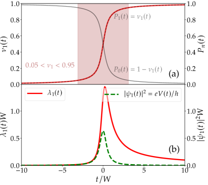
Figure 2: (a) Emission probability $\nu_{1}(t)$ (red solid curve) of the electron in the case of single leviton emission. The red region ($t/W\in[-3.1,3.1]$) marks the emission time window, which is extracted by requiring $0.05<\nu_{1}(t)<0.95$. The distribution $P_{0}(t)=1-\nu_{1}(t)$ and $P_{1}(t)=\nu_{1}(t)$ is plotted by the grey solid and black dashed curves for comparison. (b) The emission rate $\lambda_{1}(t)$ (red solid curve) of the first electron for the single leviton emission. The leviton wave function $\left|\psi_{1}(t)\right|^{2}$ is plotted by the green dashed curve for comparison.

From the FCS, the corresponding idle time distribution can be given as $\Pi_{0}(t)=1-\int^{t}_{-\infty}d\tau|\psi_{1}(\tau)|^{2}$. By using Eq. (17), the emission rate of the electron can be related to the wave function $\psi_{1}(t)$ as

$$\lambda_{1}(t)=\frac{|\psi_{1}(t)|^{2}}{1-\int^{t}_{-\infty}d\tau|\psi_{1}(\tau)|^{2}}.$$ (27)

The typical behavior $\lambda_{1}(t)$ is illustrated in Fig. 2(b) by the red solid curve. One can see that, while the modules of the wave function $|\psi_{1}(t)|^{2}$ follows instantly to the voltage pulse $V(t)$, the emission rate exhibits a different profile. It increases rapidly in the rising edge, while decays relatively slow in the falling edge. This shows that the emission is switched on by the voltage pulse $V(t)$, but it does not switch off immediately when $V(t)$ drops to zero.

Note that by using the relation $|\psi_{1}(t)|^{2}=eV(t)/h$, the emission rate can be written as

$$\lambda_{1}(t)=\frac{eV(t)/h}{1-\int^{t}_{-\infty}d\tau eV(t)/h}.$$ (28)

This can be treated as the quantum limit of the emission rate, which describes the emission of a single leviton.

III.2 Two-leviton emitter

Now let us turn to the two-leviton emitter, which can be realized by applying a Lorentzian pulse carrying two electron charges. To better clarify the basic concept of the emission rate, let us start from a more general case, when two unit-charge Lorentzian pulses are applied with the time delay $t_{c}$. In this case, the many-body state represents two levitons propagating on top of the Fermi sea, whose wave functions can be written as $\psi_{1}(t)=\sqrt{W/(2\pi)}/(t-t_{c}/2+iW/2)$ and $\psi_{2}(t)=\sqrt{W/(2\pi)}/(t+t_{c}/2+iW/2)$. It is convenient to write the many-body state in the form similar to Eq. (24). This can be done by constructing an orthonormal basis from $\psi_{1}(t)$ and $\psi_{2}(t)$ via Gram-Schmidt orthonormal procedure, which gives

$$\psi_{a}(t) = \psi_{1}(t),$$ (29)

$$\psi_{b}(t) = \frac{1}{D}\left[\psi_{2}(t)-\langle\psi_{1}|\psi_{2}\rangle\psi_{2}(t)\right].$$ (30)

Here the normalization constant $D$ can be given as $D=1-\left|\langle\psi_{1}|\psi_{2}\rangle\right|^{2}$, with $\langle\psi_{1}|\psi_{2}\rangle=\int^{+\infty}_{-\infty}d\tau\psi^{\ast}_{1}(\tau)\psi_{2}(\tau)$ being the inner product of the two wave functions. The corresponding many-body state can be given as

$$|\Psi\rangle=\psi_{a}^{\dagger}\psi_{b}^{\dagger}|F\rangle,$$ (31)

where $\psi_{\alpha}^{\dagger}=\int dt\psi_{\alpha}(t)a^{\dagger}(t)$ (with $\alpha=a,b$) represents the creation operator of the two emitted electrons. The corresponding first-order Glauber correlation function can be related to the wave functions as

$$G(t,t^{\prime})=\psi^{\dagger}_{a}(t)\psi_{a}(t^{\prime})+\psi^{\dagger}_{b}(t)\psi_{b}(t^{\prime}).$$ (32)

By solving Eqs. (18 - 23), one finds that only the first two exclusive joint densities are non-zero, which can be written as

$$f_{1}(t_{1};t) = \left|\psi_{a}(t_{1})\right|^{2}\left(1-\int^{t}_{-\infty}d\tau\left|\psi_{b}(\tau)\right|^{2}\right)+\left|\psi_{b}(t_{1})\right|^{2}\left(1-\int^{t}_{-\infty}d\tau\left|\psi_{a}(\tau)\right|^{2}\right)$$ (33)

$$\mbox{}+2\operatorname{Re}\left[\psi_{a}(t_{1})\psi^{\ast}_{b}(t_{1})\int^{t}_{-\infty}d\tau\psi_{b}(\tau)\psi^{\ast}_{a}(\tau)\right],$$

$$f_{2}(t_{1},t_{2};t) = \left|\psi_{a}(t_{1})\psi_{b}(t_{2})\right|^{2}+\left|\psi_{a}(t_{2})\psi_{b}(t_{1})\right|^{2}-2\operatorname{Re}\left[\psi_{a}(t_{1})\psi_{b}(t_{2})\psi^{\ast}_{a}(t_{2})\psi^{\ast}_{b}(t_{1})\right].$$ (34)

It is worth noting that $f_{2}(t_{1},t_{2};t)$ is just equal to the coincidence function $g_{2}(t_{1},t_{2})$, which can also be written as

$$f_{2}(t_{1},t_{2};t)=g_{2}(t_{1},t_{2})=\left|\psi_{a}(t_{1})\psi_{b}(t_{2})-\psi_{a}(t_{2})\psi_{b}(t_{1})\right|^{2}.$$ (35)

In Eqs. (33) and (34), the first and second terms correspond to the incoherence contributions, while the last terms represents the contributions from two-electron coherence. The corresponding FCS can be described by the momentum generating function:

$$\Phi(\chi)=P_{0}(t)+P_{1}(t)e^{i\chi}+P_{2}(t)e^{2i\chi}=\left[1-\nu_{1}(t)+e^{i\chi}\nu_{1}(t)\right]\left[1-\nu_{2}(t)+e^{i\chi}\nu_{2}(t)\right].$$ (36)

It corresponds to a generalized binomial process, where two electrons attempt to emit with the probabilities $\nu_{1}(t)$ and $\nu_{2}(t)$, respectively. They can be related to the wave functions $\psi_{a}(t)$ and $\psi_{b}(t)$ as

$$\nu_{1}(t) = \frac{I_{a}+I_{b}}{2}+\sqrt{\left(\frac{I_{a}-I_{b}}{2}\right)^{2}+\left|I_{ab}\right|^{2}},$$ (37)

$$\nu_{2}(t) = \frac{I_{a}+I_{b}}{2}-\sqrt{\left(\frac{I_{a}-I_{b}}{2}\right)^{2}+\left|I_{ab}\right|^{2}}.$$ (38)

The two terms $I_{a}=\int^{t}_{-\infty}d\tau\left|\psi_{a}(\tau)\right|^{2}$ and $I_{b}=\int^{t}_{-\infty}d\tau\left|\psi_{b}(\tau)\right|^{2}$ correspond to the incoherent contributions from $\psi_{a}(t)$ and $\psi_{b}(t)$, respectively. The term $I_{ab}=\int^{t}_{-\infty}d\tau\psi^{\ast}_{a}(\tau)\psi_{b}(\tau)$ represents the contributions due to the two-electron coherence. The idle time probability can be obtained from the FCS $P_{0}(t)$ [Eq. (6)], which has the form

$$\Pi_{0}(t)=P_{0}(t)=\left[1-\int^{t}_{-\infty}d\tau\left|\psi_{a}(\tau)\right|^{2}\right]\left[1-\int^{t}_{-\infty}d\tau\left|\psi_{b}(\tau)\right|^{2}\right]-\left|\int^{t}_{-\infty}d\tau\psi_{a}(\tau)\psi^{\ast}_{b}(\tau)\right|^{2},$$ (39)

where the contributions from two-electron coherence is represented by the last term. By substituting Eqs. (33), (34) and (39) into Eqs. (14) and (17), the emission rates of the two electrons can be given as

$$\lambda_{1}(t) = \frac{f_{1}(t|t)}{\Pi_{0}(t)},$$ (40)

$$\lambda_{2}(t|t_{1}) = \frac{f_{2}(t_{1},t|t)}{f_{1}(t|t)}.$$ (41)

Figure 3: (a) Wave functions of the emitted electron for $t_{c}/W=20.0$. (b) Emission probabilities $\nu_{1}(t)$ (red solid curve) and $\nu_{2}(t)$ (green dashed curve) of the first and second electrons. The black dashed and gray solid curves represent the approximation from Eq. (42) and Eq. (43), respectively. (c) The emission rate $\lambda_{1}(t)$ (red solid curve) of the first electron. The green dashed and blue dotted curves represent the contribution solely from $\psi_{a}(t)$ [Eq. (45)] and $\psi_{b}(t)$ [Eq. (46)], respectively. The black solid curve represent the incoherent summation $\lambda_{a}(t)+\lambda_{a}(t)$.

To better understand the physical meaning of the emission rates, let us first consider on a limit case, when the wave functions of two levitons are well-separated from each other. In this case, the two electrons are essentially distinguishable and one expect that their emissions can be treated as independent events. This is demonstrated in Fig. 3(a), corresponding to $t_{c}/W=20.0$. In this case, one has $\psi_{a}(t)\approx\psi_{1}(t)$ and $\psi_{b}(t)\approx\psi_{2}(t)$. The overlap between them are rather small, indicating a negligible two-electron coherence. By dropping the coherence contributions $I_{ab}$ in Eqs. (37) and (38), the emission probabilities can be well-approximated as

$$\nu_{1}(t) \approx \int^{t}_{-\infty}d\tau\left|\psi_{a}(\tau)\right|^{2},$$ (42)

$$\nu_{2}(t) \approx \int^{t}_{-\infty}d\tau\left|\psi_{b}(\tau)\right|^{2}.$$ (43)

The approximation is illustrated in Fig. 3(b). The red solid and green dash curves represent the exact result from Eqs. (37) and (38), while the black dashed and gray solid curves correspond to the approximation given in Eqs. (42) and (43), respectively. One can see that they agrees quite well, indicating that the emission of the two electron are dominated by the corresponding wave functions $\psi_{a}(t)$ and $\psi_{b}(t)$, respectively.

The independence of the emission can also be seen from the emission time windows. From Fig. 3(b), one can see that $\nu_{1}(t)$ [$\nu_{2}(t)$] increases rapidly from $0.05$ to $0.95$ as $t/W$ increases from $-12.42$ to $-5.45$ ($7.22$ to $15.47$). This indicates that the two electrons are most likely to be emitted in two time windows $t/W\in[-12.42,-5.45]$ and $t/W\in[7.22,15.47]$, which are marked by the the red and green regions in Fig. 3(b). One can see that they are well-separated from each other, indicating that the emission of the two electrons can be treated as independent events, which are distinguishable from their emission times.

Now let us discuss the emission rate $\lambda_{1}(t)$ of the first electron. From Eqs. (33), (39) and (40), one finds that both $\psi_{a}(t)$ and $\psi_{b}(t)$ can contribute to $\lambda_{1}(t)$. By dropping the coherence contributions [the last terms in Eqs. (33) and (39) ], the emission rate of the first electron $\lambda_{1}(t)$ can be approximated as

$$\lambda_{1}(t)\approx\lambda_{a}(t)+\lambda_{b}(t),$$ (44)

with

$$\lambda_{a}(t) = \frac{|\psi_{a}(t)|^{2}}{1-\int^{t}_{-\infty}d\tau|\psi_{a}(\tau)|^{2}},$$ (45)

$$\lambda_{b}(t) = \frac{|\psi_{b}(t)|^{2}}{1-\int^{t}_{-\infty}d\tau|\psi_{b}(\tau)|^{2}}.$$ (46)

By comparing to Eq. (27), one finds that these two terms are just the emission rates solely due to $\psi_{a}(t)$ and $\psi_{b}(t)$, respectively. The two terms can lead to two well-separated peaks in the emission rate $\lambda_{1}(t)$. This can be seen from Fig. 3(c). In the figure, the red solid curve represents the exact emission rate $\lambda_{1}(t)$, while the emission rates $\lambda_{a}(t)$ and $\lambda_{b}(t)$ are plotted by the green dashed and blue dotted curves, respectively. Around the first peak ($t/W=-10.0$), one finds that the emission rate $\lambda_{1}(t)$ is almost solely due to $\lambda_{a}(t)$. In contrast, although $\lambda_{b}(t)$ dominates the emission rate around the second peak ($t/W=10.0$), the two-electron coherence can also play a non-negligible role. As a consequence, the approximation from Eq. (44) slightly underestimates the exact emission rate, which can be seen by comparing the red solid curve (exact emission rate) to the black solid one [Eq. (44)]. However, as the emission of the first electron is concentrated in the emission time window of the first electron [red region in Fig. 3(b)], $\lambda_{1}(t)$ is essentially decided by $\lambda_{a}(t)$ alone.

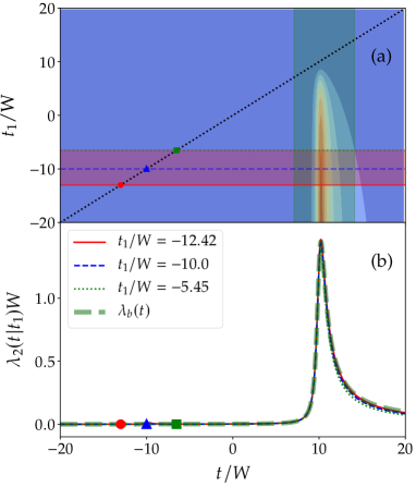
Figure 4: (a) The emission rate $\lambda_{2}(t|t_{1})$ as a contour plot in $t$-$t_{1}$ plane. It is only nonzero for $t_{1}<t$ (lower-right side of plane. The black dashed curve represents $t_{1}=t$ ). The red and green regions represent the emission time windows of the first and second electrons, respectively. (b) $\lambda_{2}(t|t_{1})$ as a function of $t$ for three typical $t_{1}$ in the first emission time window. The red solid, blue dashed and green dotted curves correspond to $t_{1}/W=-12.42$, $-10.0$ and $-5.45$. The red dots, blue triangles and green squares in both (a) and (b) mark the corresponding points $t=t_{1}$.

Now we turn to the emission rate $\lambda_{2}(t|t_{1})$ of the second electron. By dropping the coherence contributions [the last terms in Eqs. (33) and (34)], it can be approximated as

$$\lambda_{2}(t|t_{1})\approx\frac{\left|\psi_{a}(t_{1})\psi_{b}(t)\right|^{2}+\left|\psi_{a}(t)\psi_{b}(t_{1})\right|^{2}}{\left|\psi_{a}(t_{1})\right|^{2}\left(1-\int^{t}_{-\infty}d\tau\left|\psi_{b}(\tau)\right|^{2}\right)+\left|\psi_{b}(t_{1})\right|^{2}\left(1-\int^{t}_{-\infty}d\tau\left|\psi_{a}(\tau)\right|^{2}\right)}.$$ (47)

Here $t_{1}$ represents the emission time of the first electron, which satisfies $t_{1}<t$ following the restriction given in Eq. (12). Due to the $t_{1}$-dependence, the behavior of $\lambda_{2}(t|t_{1})$ appears more complicated. This can be seen from Fig. 4(a), where we plot $\lambda_{2}(t|t_{1})$ as a contour plot in the $t$-$t_{1}$ plane. Note that $\lambda_{2}(t|t_{1})$ is only nonzero in the lower-right side of the plane, which is due to the restriction $t_{1}<t$. From the contour plot, one finds that $\lambda_{2}(t|t_{1})$ exhibits a strong peak around $t/W=10.0$. The amplitudes of the peak drop to zero as $t_{1}$ approach $t$. It seems that the emission of the second electron is correlated to the first one even in the absence of two-electron coherence.

However, the $t_{1}$-dependence is essentially negligible when $t_{1}$ lies in the first emission time window, which is marked by the red region in Fig. 4(a). In this case, $\left|\psi_{b}(t_{1})\right|^{2}$ is rather small [see Fig. 3(a)] and can be omitted in Eq. (47). In doing so, one finds that $\lambda_{2}(t|t_{1})$ can be written as

$$\lambda_{2}(t|t_{1})\approx\frac{\left|\psi_{b}(t)\right|^{2}}{1-\int^{t}_{-\infty}d\tau\left|\psi_{b}(\tau)\right|^{2}}=\lambda_{b}(t).$$ (48)

It is just the emission rate solely from the wave function $\psi_{b}(t)$, which does not depends on $t_{1}$. This approximation is demonstrated in Fig. 4(b). In the figure, the red solid, blue dashed and green dotted curves corresponds to $\lambda_{2}(t|t_{1})$ with three typical $t_{1}$ in the emission time window of the first electron. The thick green dashed curve represents $\lambda_{b}(t)$. One can see that they agree quite well, indicating that the emission of the second electron is dominated by $\psi_{b}(t)$.

The above results show that when the two pulses are well-separated in the time domain, the emission of the two electrons can be treated as independent quantum events, whose emission rates are decided solely by their own wave functions.

As the two pulses approach each other, the wave function of the two electrons can overlap. This is demonstrated Fig. 5(a), corresponding to $t_{c}/W=2.0$. The emission probabilities $\nu_{1}(t)$ and $\nu_{2}(t)$ are plotted in Fig. 5(b) by the red solid and green dashed curves, respectively. In this case, the two electrons are most likely to be emitted in two time windows $t/W\in[-4.97,0.7]$ and $t/W\in[-0.53,9.4]$, which are marked by the red and green regions in Fig. 5(b). The two time windows can overlap with each other, indicating that their emissions are correlated. Indeed, one finds that the approximations for the emission probabilities Eqs. (42) (black dashed curve) and (43) (gray solid curve) becomes inaccurate, as illustrated in Fig. 5(b). This indicates that the two-electron coherence can play a non-negligible role on the emission process.

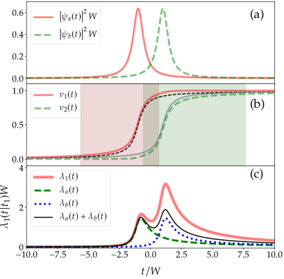
Figure 5: The same as Fig. 3 but for $t_{c}/W=2.0$.

The impact of the two-electron coherence can also be seen from the emission rate $\lambda_{1}(t)$. This is demonstrated in Fig. 5(c). The red solid curve represents the exact emission rate $\lambda_{1}(t)$, while the green dashed and blue dotted curves correspond to the emission rates solely from $\lambda_{a}(t)$ [Eq. (45)] and $\lambda_{b}(t)$ [Eq. (46)], respectively. The black solid curve represents the incoherent summation $\lambda_{a}(t)+\lambda_{b}(t)$. One can see that $\lambda_{1}(t)$ is larger than the $\lambda_{a}(t)+\lambda_{b}(t)$, which can be attributed to the contribution from the two-electron coherence.

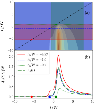
Figure 6: The same as Fig. 4 but for $t_{c}/W=2.0$. The red solid, blue dashed and green dotted curves correspond to $t_{1}/W=-4.97$, $-1.0$ and $-0.7$.

While the two-electron coherence enhances the emission rate $\lambda_{1}(t)$ of the first electron, it plays a different role for the emission rate $\lambda_{2}(t|t_{1})$ of the second electron. This can be seen from Fig. 6(a), where we plot $\lambda_{2}(t|t_{1})$ as a contour plot in the $t$-$t_{1}$ plane. One can see that $\lambda_{2}(t|t_{1})$ exhibits a strong peak around $t/W=1.0$ and a small shoulder peak around $t/W=-1.0$. The amplitudes of both peaks drop as $t_{1}$ approaches $t$. The dependence remains pronounced when $t_{1}$ lies in the first emission time window, which is marked by the red region in Fig. 6(a). The $t_{1}$-dependence can be better seen from Fig. 6(b). In the figure, the red solid, blue dashed and green dotted curves corresponds to $\lambda_{2}(t|t_{1})$ with three typical $t_{1}$ in the emission time window of the first electron. The emission rate $\lambda_{b}(t)$ solely due to $\psi_{b}(t)$ [Eq. (46)] is plotted by the thick green dashed curve for comparison. One finds that $\lambda_{b}(t)$ can only give a good estimation of $\lambda_{2}(t|t_{1})$ for $t_{1}/W=-1.0$ (blue dashed curve). In contrast, $\lambda_{2}(t|t_{1})$ is suppressed for $t_{1}/W=0.7$ (green dotted curve) and it is enhanced for $t_{1}/W=-4.97$ (red solid curve), indicating that the emission of the second electron is strongly correlated to the first one. In particular, $\lambda_{2}(t|t_{1})$ always drops to zero as $t_{1}$ approaches $t$. This is also illustrated in Fig. 6(b), where the point $t=t_{1}$ are marked by the red dot ($t_{1}/W=-4.97$), blue triangle ($t_{1}/W=-1.0$) and green square ($t_{1}/W=0.7$), respectively.

The behavior of $\lambda_{2}(t|t_{1})$ can be understood in an intuitive way. When $t_{1}/W=-1.0$, one has $|\psi_{a}(t_{1})|\gg|\psi_{b}(t_{1})|$ [see Fig. 5(a)]. Then the emission of the first electron at $t_{1}$ is almost solely due to $\psi_{a}(t_{1})$. As the first electron has been emitted, the many-body state is most likely to be collapsed to $|\Psi\rangle=\psi^{\dagger}_{b}|F\rangle$, which is just a single-electron state with wave function $\psi_{b}(t)$. This explains why one has $\lambda_{2}(t|t_{1})\approx\lambda_{b}(t)$ for $t_{1}/W=-1.0$. As $t_{1}$ approaches $t$, the Pauli exclusion principle prevents two electrons emit at the same time, which can greatly suppress the emission rate $\lambda_{2}(t|t_{1})$ when $t_{1}$ is sufficiently close to $t$. In particularly, it requires $\lambda_{2}(t_{1}|t_{1})=0$. This can be seen more clearly by substituting Eq. (35) into Eq. (41). When $t_{1}$ is far from $t$, both $\psi_{a}(t)$ and $\psi_{b}(t)$ can contribute to the emission of the second electron, while the suppression due to the Pauli exclusion principle becomes less important. As a consequence, the emission rate $\lambda_{2}(t|t_{1})$ is enhanced comparing to $\lambda_{b}(t)$.

The above results show that the two-electron coherence can have a different impact on the emission of two electrons. While it always enhances the emission rate $\lambda_{1}(t)$, its impact on $\lambda_{2}(t|t_{1})$ depends strongly on $t_{1}$. In particular, it greatly suppresses $\lambda_{2}(t|t_{1})$ when $t$ is close enough to $t_{1}$. This can be attributed to the Pauli exclusion principle, indicating a strong correlation at short times.

In the extreme case when $t_{c}/W=0$, the two voltage pulses reduce to a single pulse carrying two electron charges. In this case, the modules of the two wave functions $\psi_{a}(t)$ and $\psi_{b}(t)$ exhibit the same profile, which is shown in Fig. 7(a). But the emission of the two electrons are distributed in two time windows $t/W\in[-4.8,0.32]$ (red region) and $t/W\in[-0.3,9.3]$ (green region), which are only slightly overlapped. This can be seen from the corresponding emission probabilities plotted in Fig. 7(b).

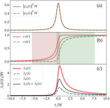
Figure 7: The same as Fig. 3 but for $t_{c}/W=0.0$.

In this case, the two-electron coherence can make a large contribution, which greatly enhances the emission rate of the first electron $\lambda_{1}(t)$. This can be seen by comparing the red solid curve to the black dotted one in Fig. 7(c). Due to the contribution from the two-electron coherence, the $t_{1}$-dependence of $\lambda_{2}(t|t_{1})$ also becomes more pronounced, which can be seen from Fig. 8.

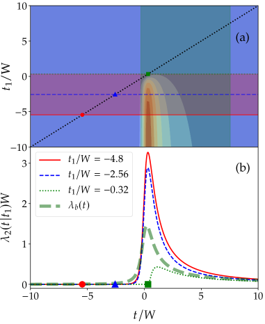
Figure 8: The same as Fig. 4 but for $t_{c}/W=0.0$. The red solid, blue dashed and green dotted curves correspond to $t_{1}/W=-4.8$, $-2.56$ and $-0.32$.

In the end of this section, let us elucidate the relation between the electron emission and driving pulse by using the emission rates. This is illustrated in Fig. 9, corresponding to $t_{c}/W=20.0$ (a), $t_{c}/W=2.0$ (b) and $t_{c}/W=0.0$ (c). In the figure, the red solid curve represents the emission rate of the first electron $\lambda_{1}(t)$. The green dotted, blue dashed and orange dashed-dotted curves represent the emission rates of the second electron $\lambda_{2}(t|t_{1})$ for three typical $t_{1}$ in the emission time window of the first electron. The normalized driving voltage $eV(t)/h$ are plotted by the black solid curve for comparison. When the two pulses are well-separated [Fig. 9(a)], one finds that the rising edges of $\lambda_{1}(t)$ [$\lambda_{2}(t|t_{1})$] follows the first [second] driving pulse. In the meantime, the emission rate $\lambda_{2}(t|t_{1})$ is almost independent on $t_{1}$. This indicates a good synchronization between the electron emissions and driving pulses. In this case, the two electrons tend to be emitted in two separated time windows (red and green regions), which are approximately centered around the peak of the each pulse. As the two pulses approach each other, the emission rate $\lambda_{1}(t)$ is greatly enhanced, leading to a fast rising edge. As a consequence, the first electron tends to be emitted before the peak of the first pulse. This can be seen by comparing the red regions in Fig. 9(a-c). In contrast, the emission rate $\lambda_{2}(t|t_{1})$ becomes $t_{1}$-dependent, which is enhanced when $t_{1}$ is far from $t$ and greatly suppressed when $t_{1}$ is close to $t$. As a consequence, the emission of the second electron tends to be emitted after the peak of the second pulse. This can be seen by comparing the green regions in Fig. 9(a-c).

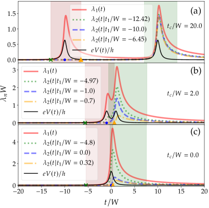
Figure 9: The relation between the emission rates $\lambda_{1}(t)$, $\lambda_{2}(t)$ and normalized driving pulse $eV(t)/h$ for $t_{c}/W=20.0$ (a), $t_{c}/W=2.0$ (b) and $t_{c}/W=0.0$ (c). The emission time windows for the first and second electrons are marked by the red and green regions. The red solid curve represents $\lambda_{1}(t)$. The green dotted, blue dashed and orange dash-dotted curves represent $\lambda_{2}(t|t_{1})$ with three typical $t_{1}$, which lie in the first emission time window.

IV Finite temperatures

Now let us discuss the impact of the finite temperature. In this case, the first-order Glauber function can be expressed as [11, 46]

$$G(t,t^{\prime}) = \sum_{i}\int d\epsilon\left[-\frac{\partial f(\epsilon)}{\partial\epsilon}\right]$$ (49)

$$\times\left[\psi_{i}(t)e^{-i\epsilon t}\right]\left[\psi_{i}(t^{\prime})e^{-i\epsilon t^{\prime}}\right]^{\dagger}.$$

For the single electron emission, one can choose $i=1$ [see Eq. (25)], while for the two electron emission, one can choose $i=a,b$ [see Eq. (32)]. Here $f(\epsilon)=1/\left[1+e^{-\epsilon/(k_{B}T)}\right]$ represents the Fermi-Dirac distribution, with $T$ being the electron temperature. Note that we set the zero of energy to be the Fermi energy in the electrode. In the calculation, we choose $T_{W}=\hbar/(k_{B}W)$ as the temperature unit.

IV.1 Single-electron emitter

Equation (49) corresponds to a mixed state. It indicates that a large number of electrons can be emitted due to thermal fluctuations [11]. Each electron is emitted with the probability $p(\epsilon)=-\partial_{\epsilon}f(\epsilon)$, whose wave function can be given as $\psi_{i}(t)e^{-i\epsilon t}$. As a consequence, even a single Lorentzian pulse can trigger the emission of multiple electrons. This can be seen from the time-resolved FCS, which is illustrated in Fig. 10. In the left column [(a-c)] of the figure, we plot emission probabilities $\nu_{\alpha}(t)$ as functions of the normalized time $t/W$. The three sub-figures (a), (b) and (c) correspond to $T/T_{W}=0.01$, $T/T_{W}=0.1$ and $T/T_{W}=1.0$, respectively. The corresponding distributions $P_{n}(t)$ are plotted in the right column [(d-f)]. For better visualization, we only show the first three distributions $P_{0}(t)$, $P_{1}(t)$ and $P_{2}(t)$, which are plotted by the thick red solid, green dotted and blue dashed curves, respectively.

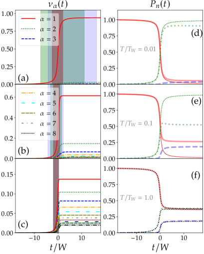
Figure 10: (a-c) Emission probabilities $\nu_{\alpha}$ ($\alpha=1,2,\dots,8$) at different temperatures. The emission is driven by a single Lorentzian pulse carrying an unit electron charge. The red, green and blue regions correspond to the emission time windows of the first three electrons. (d-f) The corresponding distributions $P_{n}(t)$. The thick red solid, green dotted and blue dashed curves represent $P_{0}(t)$, $P_{1}(t)$ and $P_{2}(t)$, respectively. The thin red solid and green dashed curves in (d) and (e) represent the quantum limit of $P_{0}(t)$ and $P_{1}(t)$ from Eq. (1). The black dashed curves in (f) represent the classical limit, corresponding to the Poisson process with emission rate $\lambda_{c}(t)=eV(t)/h$.

At low temperatures, the emission probability $\nu_{1}(t)$ plays the dominant role. For $T/T_{W}=0.01$, it can reach the maximum value $0.94$ in the long time limit $t\to+\infty$. This is illustrated by the red solid curve in Fig. 10(a). It increases from $5\%$ to $95\%$ of its maximum value for $t/W\in[-2.5,2.03]$, indicating that the emission is concentrated in this time window (marked by the red region). In contrast, other emission probabilities are rather small. In Fig. 10(a), one can only identify $\nu_{2}(t)$ (green dotted curve) and $\nu_{3}(t)$ (blue dashed curve), which merely reach $0.03$ and $0.01$ in the long time limit. The corresponding emission time windows are $t/W\in[-7.34,11.1]$ and $t/W\in[-4.22,16.33]$, which are marked by the green and blue regions in the figure. The two time windows are much wider than the emission time window of the first electron, indicating that the emission of the second and third electrons are less concentrated in the time domain. This results show that the emission due to thermal fluctuations is weak at this temperature. In fact, the corresponding distribution $P_{n}(t)$ can still be well-approximated by the quantum limit from Eq. (1), which can be seen from Fig. 10(d).

As the temperature increases to $T/T_{W}=0.1$, the emission probability $\nu_{1}(t)$ is suppressed, which can only reach $0.61$ in the long time limit [red solid curve in Fig. 10(b)]. It increases from $5\%$ to $95\%$ of its maximum value for $t/W\in[-1.95,0.7]$ [red region in Fig. 10(b)]. Comparing to Fig. 10(a), one can see that that the corresponding emission time window is narrowed. In the meantime, the emission probabilities $\nu_{2}(t)$ and $\nu_{3}(t)$ are enhanced, which can reach $0.15$ and $0.07$ in the long time limit. Their emission time windows become $t/W\in[-3.2,1.48]$ and $t/W\in[-4.3,2.19]$, which are also narrowed significantly. Comparing to Fig. 10(a), one also finds that other emission probabilities $\nu_{\alpha}(t)$ ($\alpha=4,5,\dots,8$) can have non-negligible contributions. This makes the distribution $P_{n}(t)$ departs from the quantum limit, as illustrated in Fig. 10(e).

As the temperature $T$ further increases, more emission probabilities can contribute. This is illustrated in Fig. 10(c), corresponding to $T/T_{W}=1.0$. From the figure, one finds that the emission is not dominated by a single probability. Instead, there exits a large number of emission probabilities, which are comparable in magnitude. This makes the corresponding distribution $P_{n}(t)$ approaches the time-dependent Poisson distribution from Eq. (2). This can be seen from Fig. 10(f), where the Poisson distribution is plotted by the black dotted curves. At this temperature, the emission time windows of the first three electrons are almost completely overlapped, which can be seen by comparing the red, green and blue regions in Fig. 10(c). This suggests that all the electron tends to be emitted in the same time window at high temperatures.

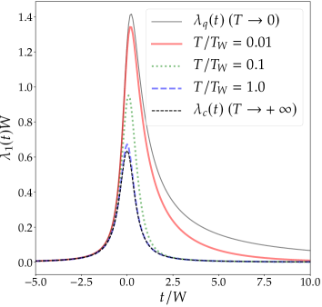
Figure 11: Emission rate $\lambda_{1}(t)$ of the first electron at different temperatures. The gray solid curve corresponds to the quantum limit from Eq. (28), while the black dashed curve corresponds to the classical limit $\lambda_{c}(t)=eV(t)/h$.

The above results indicate that the system can be treated as a Poisson emitter at high temperatures, whose emission rate follows the driving pulse as $\lambda_{c}(t)=eV(t)/h$. We find that the emission rate $\lambda_{1}(t)$ of the first electron does evolve from the quantum limit $\lambda_{q}(t)$ from Eq. (28) (gray solid curve) to the classical limit $\lambda_{c}(t)$ (black dotted curve) as the temperature $T$ increases from zero to $T_{W}$, which is plotted in Fig. 11.

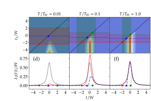
Figure 12: (a-c) Emission rate $\lambda_{2}(t|t_{1})$ at different temperatures, which are plotted as contour plots in the $t$-$t_{1}$ plane. The red and green regions mark the emission time windows of the first and second electrons. (d-f) $\lambda_{2}(t|t_{1})$ as a functions of $t$ at different temperatures for three typical $t_{1}$ lies in the emission time windows of the first electron. In (d), the red solid, blue dashed and green dotted curves correspond to $t_{1}/W=-2.5$, $-0.23$ and $2.03$, respectively. In (e), the red solid, blue dashed and green dotted curves correspond to $t_{1}/W=-1.95$, $-0.63$ and $0.7$, respectively. In (e), the red solid, blue dashed and green dotted curves correspond to $t_{1}/W=-1.95$, $-0.9$ and $0.16$, respectively. The point $t=t_{1}$ are marked by the red dots, blue triangles and green squares. The black dotted curves represent the classical limit $\lambda_{c}(t)=eV(t)/h$.

However, the Poissonian character from $P_{n}(t)$ and $\lambda_{1}(t)$ does not mean that the emission events are completely uncorrelated. This can be seen from the emission rate $\lambda_{2}(t|t_{1})$ of the second electron, which is illustrated in Fig. 12. In the figure, we compare $\lambda_{2}(t|t_{1})$ at three typical temperatures $T/T_{W}=0.01$ (a), $T/T_{W}=0.1$ (b) and $T/T_{W}=1.0$ (c), which are plotted as contour plots in the $t$-$t_{1}$ plane. The emission time windows for the first and second two electrons are also shown by the red and green regions in the $t$-$t_{1}$ plane. As the emission of the second electron is the coeffect of the driving pulse and thermal fluctuations, it remains very weak at low temperatures. This is illustrated in Fig. 12(a), corresponding to $T/T_{W}=0.01$. In this case, $\lambda_{2}(t|t_{1})$ is much smaller than the classical limit $\lambda_{c}(t)$. This can be seen from Fig. 12(d), where we compare $\lambda_{2}(t|t_{1})$ with three typical times $t_{1}$ to the classical limit $\lambda_{c}(t)$ (black dotted curve). Note that at this temperature, the emission time window of the second electron is rather wide. It corresponds to $t/W\in[-7.34,11.1]$, which covers the whole range of $t/W$-axis.

The emission rate $\lambda_{2}(t|t_{1})$ increases rapidly as the temperature reaches $T/T_{W}=0.1$. This can be seen by comparing Fig. 12(b) to Fig. 12(a). This suggests that the emission of the second electron is enhanced by thermal fluctuations. In the meantime, it is still strongly correlated to the emission of the first electron. This is better illustrated in Fig. 12(e), where we plot $\lambda_{2}(t|t_{1})$ with three typical times $t_{1}/W=-1.95$, $-0.63$ and $0.7$ by the red solid, blue dashed and green dotted curves, respectively. One can see that $\lambda_{2}(t|t_{1})$ depends strongly on the value of $t_{1}$. In particular, it drops rapidly to zero as $t$ approaches $t_{1}$, where the points corresponding to $t=t_{1}$ are marked by the red dot ($t_{1}/W=-1.95$), blue triangle ($t_{1}/W=-0.63$) and green square ($t_{1}/W=0.7$). This indicates that the correlation due to the Pauli exclusion principle is still preserved at this temperature. The correlation remains pronounced at high temperatures. This is demonstrated in Fig. 12(c), corresponding to $T/T_{W}=1.0$. At this temperature, one finds that $\lambda_{2}(t|t_{1})$ largely follows $\lambda_{c}(t)$ when $t>t_{1}$, but drops to zero rapidly as $t$ approaches $t_{1}$. The relation between $\lambda_{2}(t|t_{1})$ and $\lambda_{c}(t)$ is better illustrated in Fig. 12(f), where we plot $\lambda_{2}(t|t_{1})$ with three typical $t_{1}$ by the red solid, green dotted and blue dashed curves, while $\lambda_{c}(t)$ is plotted by the black dotted curve for comparison.

Although the correlations are always present, they can only play a non-negligible role at short times. To better seen this, we plot the emission rates $\lambda_{2}(t|t_{1})$ as a function of $t_{1}/W$ in Fig. 13, where subfigures (a), (b) and (c) correspond to three typical emission time $t/W=-1.0$, $-0.5$ and $0.0$, respectively. One can see that $t_{1}$ can only affect the emission rate $\lambda_{2}(t|t_{1})$ when $t_{1}$ is close enough to $t$. If $t_{1}$ is too far from $t$, i.e., $t-t_{1}>\tau_{c}$, $\lambda_{2}(t|t_{1})$ is almost a constant, indicating the absence of the correlation at long times. Here $\tau_{c}$ can be regarded as a correlation time, which should depends on both the temperature $T$ and the emission time $t$. We estimate the value of $\tau_{c}$ by requiring that

$$\frac{\lambda_{2}(t|t_{1}\to-\infty)-\lambda_{2}(t|t_{1})}{\lambda_{2}(t|t_{1}\to-\infty)}<0.05$$ (50)

when $t-t_{1}>\tau_{c}$. In doing so, we obtain $\tau_{c}$ as a function of normalized temperature $T/T_{W}$ for three typical emission time $t$. This is shown in the inset of Fig. 13, where different curves corresponds to different $t$. One can see that $\tau_{c}$ for different $t$ exhibits similar temperature dependence, which drops to zero rapidly as the temperature $T/T_{W}$ increases. This results show that, although the correlations are always present, they are difficult to be observed at high temperatures due to the short correlation times. As a consequence, the emission rate $\lambda_{2}(t|t_{1})$ tends to follow the classical limit $\Theta(t-t_{1})eV(t)/h$, which is plotted by the gray solid curves in Fig. 13.

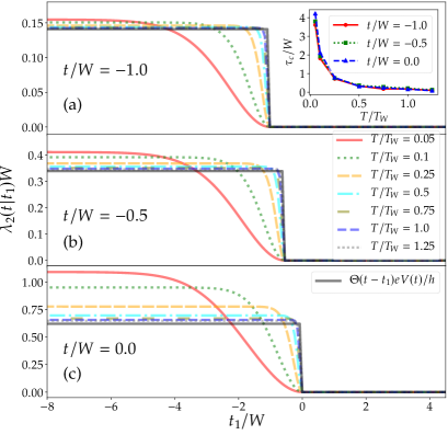
Figure 13: Emission rate $\lambda_{2}(t|t_{1})$ as a function of $t_{1}/W$ for three typical $t/W=-1.0$ (a), $-0.5$ (b) and $0.0$ (c). Curves with different colors and line types correspond to different temperatures. The gray solid curve represent the classical limit $\Theta(t-t_{1})eV(t)/h$. The inset shows the correlation times $\tau_{c}$ as a function of temperature $T/T_{W}$.

The above results show that thermal fluctuations in the electrode can suppress the correlations, making the emission process behaves like a time-dependence Poisson process at long times. As these results are obtained in the case of single Lorentzian pulse, one may wonder if such conclusion still holds in more general cases. To further confirm our conclusion, in the next subsection we consider the case when a Lorentzian pulse carrying two electric charges are applied on the electrode.

IV.2 Two-electron emitter

This corresponds to the case $t_{c}/W=0$ discussed in Sec. III.2. The typical behavior of the FCS is demonstrated in Fig. 14. Comparing to Fig. 10, one can identify the same features as the temperature $T$ reaches $T_{W}$: 1) The distribution $P_{n}(t)$ evolves from the quantum limit [thin colored curves in Fig. 14(d) and (e)] to the classical limit [thin dotted curves in Fig. 14(f)]. Note that in this case, the quantum limit of $P_{n}(t)$ is calculated from Eq. (36). There are three non-zero distributions $P_{0}(t)$, $P_{1}(t)$ and $P_{2}(t)$, which are plotted by thin red solid, green dotted and blue dashed curves, respectively. 2) Multiple electrons can be emitted due to thermal fluctuations, which tends to be emitted in the same time window [the colored region in Fig. 14(c)]. These features indicates that the quantum-to-classical crossover exhibit same behavior as in the case of unit-charged pulse.

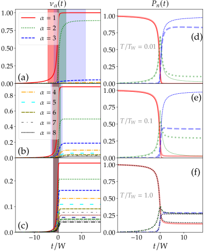
Figure 14: The same as Fig. 10 but with the driving pulse carrying two electron charge. In this case, the quantum limit of $P_{n}(t)$ is obtained from Eq. (36). The thin red solid, green dotted and blue dashed curves in (d) and (e) correspond to $P_{0}(t)$, $P_{1}(t)$ and $P_{2}(t)$, respectively.

The similarity of the crossover can also be seen from the emission rates. In Fig. 15. One can see that the emission rate $\lambda_{1}(t)$ of the first electron evolves from the quantum limit to the classical limit $\lambda_{c}(t)=eV(t)/h$ as temperature $T$ approaches $T_{W}$. Note that in this case, the quantum limit $\lambda_{q}(t)$ is calculated from Eq. (40). In the meantime, the emission rate $\lambda_{2}(t|t_{1})$ of the second electron tends to follow the classical counterpart $\Theta(t-t_{1})eV(t)/h$, which is illustrated in Fig. 16 and 17. Moreover, we also compare the temperature-dependence correlations time $\tau_{c}$ in the two cases, which are illustrated in Fig. 18. In the figure, the curves with the label “$1e$” represent the correlation times from the inset of Fig. 13, while curves with the label “$2e$” represent the correlation times from the inset of Fig. 17. One finds that they tends to follow the same temperature dependence. These results indicates that the quantum-to-classical crossover exhibit similar behavior, despite the voltage pulse carrying one or two electron charges.

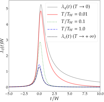
Figure 15: The same as Fig. 11 but with the driving pulse carrying two electron charge. In this case, the classical limit $\lambda_{c}(t)$ still follows $eV(t)/h$, but the quantum limit $\lambda_{q}(t)$ is determined from Eq. (40).

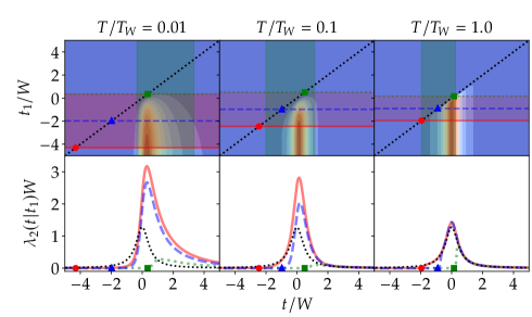
Figure 16: The same as Fig. 12 but with the driving pulse carrying two electron charge.

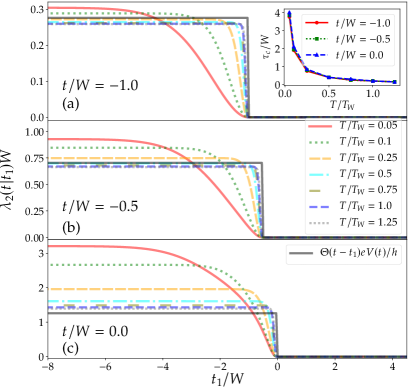
Figure 17: The same as Fig. 13 but with the driving pulse carrying two electron charge.

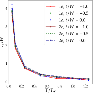
Figure 18: The correlation time $\tau_{c}$ as a function of temperature $T/T_{W}$. Curves with the label “$1e$” represent the correlation times from the inset of Fig. 13, while curves with the label “$2e$” represent the correlation times from the inset of Fig. 17.

V Summary and Discussion

In summary, we have investigated the quantum-to-classical crossover in a single-electron emitter, which is driven by electrode temperature. By combining the time-resolved FCS and emission rates, we have shown that the emission approaches a time-dependence Poisson process at long times. In contrast, the correlation between emission events remains at short times, which is due to the Pauli exclusion principle. This behavior is demonstrated in two cases, when the electron emission is driven by a Lorentzian pulse carrying a single and two electron charges.

It is worth noting that the quantum-to-classical crossover has also been studied previously in another type of single-electron emitter [47], which is based on a driven localized state [48, 49, 50]. Instead of increasing the temperature, the quantum-to-classical crossover in such emitter is realized by manipulating the driving rate of the localized state. The quantum-to-classical crossover is characterized via the Wigner function [51, 52]. The emitted electron from such emitter can have a energy which is far above the Fermi level, whose Wigner function can be partially resolved from a continuous-variable tomography techniques [53]. It will be interesting to study the quantum-to-classical crossover in such emitter by using our approach, which we will explore in future works.