Policy iteration: for want of recursive feasibility, all is not lost

Abstract

This paper investigates recursive feasibility, recursive robust stability and near-optimality properties of policy iteration (PI). For this purpose, we consider deterministic nonlinear discrete-time systems whose inputs are generated by PI for undiscounted cost functions. We first assume that PI is recursively feasible, in the sense that the optimization problems solved at each iteration admit a solution. In this case, we provide novel conditions to establish recursive robust stability properties for a general attractor, meaning that the policies generated at each iteration ensure a robust $\mathcal{KL}$-stability property with respect to a general state measure. We then derive novel explicit bounds on the mismatch between the (suboptimal) value function returned by PI at each iteration and the optimal one. Afterwards, motivated by a counter-example that shows that PI may fail to be recursively feasible, we modify PI so that recursive feasibility is guaranteed a priori under mild conditions. This modified algorithm, called PI⁺, is shown to preserve the recursive robust stability when the attractor is compact. Additionally, PI⁺ enjoys the same near-optimality properties as its PI counterpart under the same assumptions. Therefore, PI⁺ is an attractive tool for generating near-optimal stabilizing control of deterministic discrete-time nonlinear systems.

1 Introduction

Policy iteration (PI) is an optimization algorithm that forms one of the pillars of dynamic programming [2]. PI iteratively generates control laws, also called policies, that converge to an optimal control law for general dynamical systems and cost functions under mild conditions, see, e.g., [2, 15, 5, 17]. Also, PI may exhibit the attractive feature of converging faster to the optimal value function than its counterpart value iteration (VI) [15] at the price of more computations. For these reasons, PI attracts a lot of attention both in terms of theoretical investigations see, e.g., [15, 3, 23, 5, 24, 7], and practical applications e.g., [29, 30, 22, 14]. Nevertheless, several fundamental questions remain largely open regarding the properties of PI in a control context: (i) its recursive feasibility; (ii) general conditions for recursive robust stability when the attractor is not necessarily a single point but a more general set; (iii) near-optimality guarantees, in particular when the cost function is not discounted. We explain each of these challenges next.

It is essential that PI is recursively feasible in the sense that the optimization problem admits a solution at each iteration. Surprisingly, we have not been able to find general conditions for the recursive feasibility of PI in the literature when dealing with deterministic nonlinear discrete-time systems with general cost functions, whose state and inputs evolves on a Euclidean space. The only results we came across concentrate on special cases like when the input set is finite [3] or the system is linear and the cost is quadratic [2]. The dominant approach in the literature for nonlinear discrete-time systems on Euclidean spaces is thus to assume that the algorithm is recursively feasible, see, e.g., [15, 23], or to rely on conditions that are hard to verify a priori in general as they employ feasibility tests at each iteration [3]. Model predictive control literature recognised a long time ago the importance of recursive feasibility. Hence we believe that the recursive feasibility of PI is a property of major importance in view of the burgeoning literature on dynamic programming and reinforcement learning where PI plays a major role [6, 4].

A second challenge for PI is related to its application in a control context. In many applications, the closed-loop system must exhibit stability guarantees as: (i) it provides analytical guarantees on the behavior of the controlled system solutions as time evolves; (ii) it endows the system with robustness properties and is thus associated to safety considerations, see, e.g., [1]. Available results on the stability of systems controlled by PI concentrate on the case where the attractor is a single point, as in, e.g., [5, 24, 7, 23]. They exclude set stability, which is inevitable for instance in presence of clock or toggle variables [9, Examples 3.1-3.2], and more generally when the desired operating behaviour of the closed-loop system is given by a set and not a point. Moreover, the commonly used assumptions imposed on the plant model and the stage cost are also subject to some conservatism, like requiring the stage cost to satisfy positive definiteness properties. In addition, it is essential to ensure that these stability properties are robust, which is not automatically guaranteed, as pointed out in [12, 21], and this matter is often eluded in the literature at the exception of the recent work in [25] in the linear quadratic case. There is therefore a need for general conditions allowing to conclude robust set stability properties for systems controlled by PI. We further would like these stability properties to be preserved at each iteration; that is, we want to ensure recursive robust stability.

Finally, it is important to understand when and how the sequence of value functions generated by PI at each iteration converges to the optimal value function; we talk of near-optimality guarantees. The literature stands in two ways on this issue. On the one hand, the value functions are known to converge monotonically and point-wisely to the optimal value function under mild conditions on the model and the cost [5, 15]; uniform convergence properties are only ensured, as far as we know, for discounted costs functions [2]. On the other hand, it is important to be able to evaluate the mismatch between the returned value function at each iteration and the optimal one. These computable or explicit bounds on the mismatch of generated value functions are vital to decide when to stop iterating the algorithm. Existing results concentrate on discounted costs [2], which are not always natural in control applications. In the discounted setting, the provided near-optimality bounds explode when the discount factor $\gamma\in(0,1)$ converges to one [2], while to ensure stability, in opposition, $\gamma$ should be close enough to one in view of [26, 11]. Hence, there is a need for stronger near-optimality guarantees for PI. In particular, we seek to develop results that provide computable near-optimality bounds, without relying on a discount factor, and to provide conditions under which the sequence of constructed value functions satisfies a uniform monotonic convergence property towards the optimal one.

In this context, we consider deterministic nonlinear discrete-time systems, whose inputs are generated by PI for an undiscounted infinite-horizon cost function. We first assume that PI is recursively feasible and we provide general conditions inspired from the model predictive control literature [13] to ensure the recursive robust stability of the closed-loop system at each iteration, where the attractor is a set. These conditions relate to the detectability of the system with respect to the stage cost and the stabilizing property of the initial policy. We then exploit these stability properties to derive explicit and computable bounds on the mismatch between the optimal value function and the value function obtained by PI at each iteration. We also show that the sequence of value functions satisfies a uniform convergence property towards the optimal value function by exploiting stability.

Afterwards, we show via a counter-example that PI may actually fail to be recursively feasible under commonly used assumptions. We thus propose to modify the original formulation of PI so that we can guarantee the recursive feasibility of the algorithm under mild conditions on the model, the stage cost and the input set. We call this new algorithm PI plus (PI⁺). PI⁺ differs from PI in two aspects. First, an (outer semicontinuous) regularization is performed at the so-called improvement step, which is a common technique in the discontinuous/hybrid systems literature [9]. Second, instead of letting the algorithm select any policy that minimizes the (regularized) improvement step, we select any of those generating the smallest cost that we aim to minimize thereby requiring an extra layer of computation. In this paper, we do not address the question of the practical implementation of PI⁺, which is left for future work. Instead, we concentrate on the methodological challenges raised by the algorithm. We then prove that PI⁺ is indeed recursively feasible, and that it preserves the recursive robust stability when the attractor is compact as well as the near-optimality properties established for PI. Compared to our preliminary work in [10], novel elements include the results for PI, the robust stability analysis, the fact that the admissible input set can be state-dependent, and new technical developments to derive less conservative near-optimality bounds. Moreover, the full proofs are provided.

The rest of the paper is organized as follows. Preliminaries are given in Section 2. The analysis of PI is carried out in Section 3. The new algorithm PI⁺ and its properties are presented in Section 4. We defer the robustness analysis of the stability properties ensured by PI and PI⁺ in Section 5. Concluding remarks are provided in Section 6. In order to streamline the presentation, the proofs are given in the appendices.

2 Preliminaries

In this section, we define the notation, provide important definitions and formalize the problem.

2.1 Notation

Let $\mathbb{R}:=(-\infty,\infty)$, $\mathbb{R}_{\geq 0}:=[0,\infty)$, $\overline{\mathbb{R}}:=[-\infty,\infty]$, $\mathbb{Z}_{\geq 0}:=\{0,1,2,\ldots\}$ and $\mathbb{Z}_{>0}:=\{1,2,\ldots\}$. The notation $(x,y)$ stands for $[x^{\top},\,y^{\top}]^{\top}$, where $x\in\mathbb{R}^{n}$, $y\in\mathbb{R}^{m}$ and $n,m\in\mathbb{Z}_{>0}$. The Euclidean norm of a vector $x\in\mathbb{R}^{n}$ with $n\in\mathbb{Z}_{>0}$ is denoted by $|x|$ and the distance of $x\in\mathbb{R}^{n}$ to a non-empty set $\mathcal{A}\subseteq\mathbb{R}^{n}$ is denoted by $|x|_{\mathcal{A}}:=\inf\{|x-y|\,:\,y\in\mathcal{A}\}$. The unit closed ball of $\mathbb{R}^{n}$ for $n\in\mathbb{Z}_{>0}$ centered at the origin is denoted by $\mathbb{B}$. We consider $\mathcal{K}$, $\mathcal{K}_{\infty}$ and $\mathcal{KL}$ functions as defined in [9, Section 3.5]. We write $\beta\in{\exp}{-}\mathcal{KL}$ when $\beta(s_{1},s_{2})=\lambda_{1}s_{1}e^{-\lambda_{2}s_{2}}$ for some $\lambda_{1}\in[1,\infty)$ and $\lambda_{2}>0$ for any $(s_{1},s_{2})\in\mathbb{R}_{\geq 0}^{2}$. For any set $\mathcal{A}\subseteq\mathbb{R}^{n}$, $x\in\mathbb{R}^{n}$, the indicator function $\delta_{\mathcal{A}}:\mathbb{R}^{n}\to\overline{\mathbb{R}}$ is defined as $\delta_{\mathcal{A}}(x)=0$ when $x\in\mathcal{A}$ and $\delta_{\mathcal{A}}(x)=\infty$ when $x\notin\mathcal{A}$ as in [27]. Moreover, when $\mathcal{A}$ is closed, we say $\sigma:\mathbb{R}^{n}\to\mathbb{R}_{\geq 0}$ is a proper indicator of set $\mathcal{A}$ whenever $\sigma$ is continuous and there exist $\underline{\alpha}_{\sigma},\overline{\alpha}_{\sigma}\in\mathcal{K}_{\infty}$ such that $\underline{\alpha}_{\sigma}(|x|_{\mathcal{A}})\leq\sigma(x)\leq\overline{\alpha}_{\sigma}(|x|_{\mathcal{A}})$ for any $x\in\mathbb{R}^{n}$. The identity map from $\mathbb{R}_{\geq 0}$ to $\mathbb{R}_{\geq 0}$ is denoted by $\mathbb{I}$, and the zero map from $\mathbb{R}_{\geq 0}$ to $0$ by $\bm{0}$. Let $f:\mathbb{R}_{\geq 0}\to\mathbb{R}_{\geq 0}$. We use $f^{(k)}$ for the composition of function $f$ to itself $k$ times, where $k\in\mathbb{Z}_{\geq 0}$ and $f^{(0)}:=\mathbb{I}$. Given a set-valued map $S:\mathbb{R}^{n}\rightrightarrows\mathbb{R}^{m}$, a selection of $S$ is a single-valued mapping $s:\text{dom}\,S\to\mathbb{R}^{m}$ such that $s(x)\in S(x)$ for any $x\in\text{dom}\,S$. For the sake of convenience, we write $s\in S$ to denote a selection $s$ of $S$. We also employ the following definition from [27, Def. 1.16].

Definition 1 (uniform level boundedness)

A function $f:\mathbb{R}^{n}\times\mathbb{R}^{m}\to\overline{\mathbb{R}}$ where $n,m\in\mathbb{Z}_{>0}$ with values $f(x,u)$ is level-bounded in $u$, locally uniform in $x$ if for each $x\in\mathbb{R}^{n}$ and $\alpha\in\mathbb{R}$ there is a neighborhood $\mathcal{S}$ of $x$ along a bounded set $B\subset\mathbb{R}^{n}$ such that $\{u\in\mathbb{R}^{m}\,:\,f(z,u)\leq\alpha\}\subset B$ for any $z\in\mathcal{S}$. $\hfill\Box$

2.2 Plant model and cost function

Consider the plant model

$$x(k+1)=f(x(k),u(k)),$$ (1)

where $x\in\mathbb{R}^{n_{x}}$ is the state, $u\in\mathcal{U}(x)\subseteq\mathbb{R}^{n_{u}}$ is the control input, the time-step is $k\in\mathbb{Z}_{\geq 0}$, $\mathcal{U}(x)$ is a non-empty set of admissible inputs for state $x\in\mathbb{R}^{n_{x}}$, and $n_{x},n_{u}\in\mathbb{Z}_{>0}$. We wish to find, for any given $x\in\mathbb{R}^{n_{x}}$, an infinite-length sequence of admissible inputs $\bm{u}=(u(0),u(1),\dots)$, that minimizes the infinite-horizon cost

$$J(x,\bm{u}):=\sum_{k=0}^{\infty}\ell(\phi(k,x,\bm{u}|_{k}),u(k)),$$ (2)

where $\ell:\mathbb{R}^{n_{x}}\times\mathbb{R}^{n_{u}}\to\mathbb{R}_{\geq 0}$ is a non-negative stage cost and $\phi(k,x,\bm{u}|_{k})$ is the solution to (1) at the $k^{\text{th}}$-step, initialized at $x$ at time 0 with inputs $\bm{u}|_{k}:=(u(0),\ldots,u({k-1}))$. The minimum of $J(x,\cdot)$ is denoted as

$$V^{\star}(x):=\min_{\bm{u}}J(x,\bm{u})$$ (3)

for any $x\in\mathbb{R}^{n_{x}}$, where $V^{\star}$ is the optimal value function associated to the minimization of (2).

Standing Assumption 1 (1)

For any $x\in\mathbb{R}^{n_{x}}$, there exists an optimal sequence of admissible inputs $\bm{u}^{\star}(x)$ such that $V^{\star}(x)=J(x,\bm{u}^{\star}(x))<{+\infty}$ and for any infinite-length sequence of admissible inputs $\bm{u}$, $V^{\star}(x)\leq J(x,\bm{u})$. $\Box$

Conditions to ensure 1 can be found in, e.g., [19]. Given (3), we define the set of optimal inputs as

$$H^{\star}(x):=\operatorname*{\text{argmin}\,}_{u\in\mathcal{U}(x)}\left\{\ell(x,u)+V^{\star}(f(x,u))\right\}.$$ (4)

To compute $H^{\star}$ in (4) for the general dynamics in (1) is notoriously hard. Dynamic programming provides algorithms to iteratively obtain feedback laws, which instead converge to $H^{\star}$ [4]. A fundamental algorithm of dynamic programming is PI, which is presented and analysed in the next section. Before that, we introduce some notation, which will be convenient in the sequel. Given a feedback law $h:\mathbb{R}^{n_{x}}\to\mathbb{R}^{n_{u}}$ that is admissible, i.e., $h\in\mathcal{U}$, we denote the solution to system (1) in closed-loop with feedback law $h$ at time $k\in\mathbb{Z}_{\geq 0}$ with initial condition $x$ at time 0 as $\phi(k,x,h)$. Likewise, $J(x,h)$ is the cost induced by $h$ at initial state $x$, i.e., $J(x,h)=\sum_{k=0}^{\infty}\ell(\phi(k,x,h),h(\phi(k,x,h)))$. In this way, we have that for any selection $h^{\star}\in H^{\star}$, $V^{\star}(\cdot)=J(\cdot,h^{\star})$, as $H^{\star}(x)$ is non-empty for any $x\in\mathbb{R}^{n_{x}}$ by 1.

3 Policy Iteration

We recall in this section the original formulation of PI and we assume the algorithm is feasible at any iteration. We then establish novel recursive stability and near-optimality guarantees, assuming a detectability property is satisfied and the initial policy is stabilizing. Finally, we present an example where PI is not recursively feasible despite supposedly favorable properties, thereby motivating the need to modify PI to overcome this issue, which will be the topic of Section 4. As mentioned in the introduction, the robustness of the stability properties is analyzed in Section 5.

3.1 The algorithm

PI is presented in 1. Given an initial admissible policy $h^{0}$, PI generates at each iteration $i\in\mathbb{Z}_{\geq 0}$ a policy $h^{i+1}$ with cost $V^{i+1}(x):=J(x,h^{i+1})$ and it can be proved that $V^{i+1}(x)\leq V^{i}(x)$ for all $x\in\mathbb{R}^{n_{x}}$ [28, Section 4.2]. This is done via the improvement step in (PI.2). The policy $h^{i+1}$ obtained at iteration $i+1$ is an arbitrary selection of $H^{i+1}$ in (PI.2) where $H^{i+1}$ may be set-valued. We then evaluate the cost induced by $h^{i+1}$, namely $V^{i+1}=J(\cdot,h^{i+1})$, this is the evaluation step in (PI.3). By doing so repeatedly, $V^{i}$ converges to the optimal value function $V^{\infty}=V^{\star}$ under mild conditions, see [2].

Algorithm 1 Policy Iteration (PI)

1:$f$ in (1), $\ell$ in (2), initial policy $h^{0}\in\mathcal{U}$

2:Policy $h^{\infty}$, cost $V^{\infty}$

3:Initial evaluation step: for all $x\in\mathbb{R}^{n_{x}}$,

$$V^{0}(x):=J(x,h^{0}).$$ (PI.1)

4:for $i\in\mathbb{Z}_{\geq 0}$ do

5:   Policy improvement step: for all $x\in\mathbb{R}^{n_{x}}$,

$$H^{i+1}(x):=\operatorname*{\text{argmin}\,}\limits_{u\in\mathcal{U}(x)}\{\ell(x,u)+V^{i}(f(x,u))\}.$$ (PI.2)

6:   Select $h^{i+1}\in H^{i+1}$.

7:   Policy evaluation step: for all $x\in\mathbb{R}^{n_{x}}$,

$$V^{i+1}(x):=J(x,h^{i+1}).$$ (PI.3)

8:end for

9:return $h^{\infty}\in H^{\infty}$ and $V^{\infty}$.

Remark 1

In practice, PI is often stopped at some iteration, typically by looking at the difference between $V^{i}$ and $V^{i-1}$ for some $i\in\mathbb{Z}_{>0}$. We will return to this point in 2 in Section 3.4.2. $\Box$

3.2 Desired properties

For the remainder of this section, we proceed as is often done in the literature and assume 1 is recursively feasible, see, e.g., [15, 23], in the sense that the optimization problem in (PI.2) admits a solution for any $x\in\mathbb{R}^{n_{x}}$ at any iteration $i\in\mathbb{Z}_{>0}$, which is formalized below.

Assumption 1

Set-valued map $H^{i}(x)$ is non-empty for any $i\in\mathbb{Z}_{>0}$ and $x\in\mathbb{R}^{n_{x}}$. $\Box$

We note that verifying 1 is hard in general. At a given iteration $i+1$ with $i\in\mathbb{Z}_{\geq 0}$, a sufficient condition for $H^{i+1}(x)$ to be non-empty for any $x\in\mathbb{R}^{n_{x}}$ is establishing the lower semicontinuity of map $(x,u)\mapsto\ell(x,u)+V^{i}(f(x,u))+\delta_{\mathcal{U}(x)}(u)$ on $\mathbb{R}^{n_{x}}\times\mathbb{R}^{n_{u}}$, see, e.g., [3]. However, this is hard to check in advance as $V^{i}$ is not known a priori. We will return to the question of the recursive feasibility of PI in Section 3.5.

Under 1, the goal of this section is to establish the recursive stability and near-optimality bounds for PI, in particular we aim at showing that PI is

• recursively stabilizing, i.e., if $h^{0}$ stabilizes system (1), then this property is also ensured by any $h^{i}\in H^{i}$ for any $i\in\mathbb{Z}_{>0}$, in the sense that the difference inclusion

  $$x(k+1)\in f(x(k),H^{i}(x(k)))=:F^{i}(x(k))$$ (5)

  exhibits desirable set stability properties;

• near-optimal in the sense that we have guaranteed bounds on $V^{i}-V^{\star}$ for any $i\in\mathbb{Z}_{\geq 0}$, despite the fact that $V^{\star}$ in (3) is typically unknown.

These results rely on assumptions given in the next section. For convenience, solutions to system (5) are denoted in the sequel as $\phi^{i}(\cdot,x)$ when initialized at some $x\in\mathbb{R}^{n_{x}}$ for any $i\in\mathbb{Z}_{\geq 0}$.

3.3 Standing assumptions

To define stability, we use a continuous function $\sigma:\mathbb{R}^{n_{x}}\to\mathbb{R}_{\geq 0}$ that serves as a state “measure” relating the distance of the state to a given attractor where $\sigma$ vanishes. By stability, we mean that there exists $\beta\in\mathcal{KL}$ (independent of $i$) such that, for any $x\in\mathbb{R}^{n_{x}}$, $i\in\mathbb{Z}_{\geq 0}$, any solution $\phi^{i}$ to (5) verifies, for any $k\in\mathbb{Z}_{\geq 0}$,

$$\sigma(\phi^{i}(k,x))\leq\beta(\sigma(x),k).$$ (6)

Property (6) is a $\mathcal{KL}$-stability property of system (5) with respect to $\sigma$. When $\sigma$ is a proper indicator function of a closed set $\mathcal{A}\subseteq\mathbb{R}^{n_{x}}$, the uniform global asymptotic stability of set $\mathcal{A}=\{x\in\mathbb{R}^{n_{x}}\,:\,\sigma(x)=0\}$ is guaranteed by (6). When $\sigma(x)=|x|^{a}$ for any $x\in\mathbb{R}^{n_{x}}$ with $a\geq 1$, the uniform global asymptotic stability of the origin $x=0$ is ensured by (6), for instance. Function $\sigma$ is thus convenient to address stability properties for general attractors.

We make the next detectability assumption on system (1) and stage cost $\ell$ consistently with e.g., [13, 26, 11, 18].

Standing Assumption 2 (2)

There exist a continuous function $W:\mathbb{R}^{n_{x}}\to\mathbb{R}_{\geq 0}$, $\alpha_{W},\chi_{W}\in\mathcal{K}_{\infty}$ and $\overline{\alpha}_{W}:\mathbb{R}_{\geq 0}\to\mathbb{R}_{\geq 0}$ continuous, nondecreasing and zero at zero, such that, for any $(x,u)\in\mathcal{W}:=\{(x,u)\in\mathbb{R}^{n}\times\mathbb{R}^{m}\,:\,u\in\mathcal{U}(x)\}$,
$$\begin{split}W(x)&{}\leq\overline{\alpha}_{W}(\sigma(x))\\ W(f(x,u))-W(x)&{}\leq-\alpha_{W}(\sigma(x))+\chi_{W}(\ell(x,u)).\end{split}$$ (7) $\Box$

2 is a detectability property of system (1) and stage cost $\ell$, see [13, 16] for more details. 2 holds for instance with $W=0$ when $\{x\in\mathbb{R}^{n_{x}}\,:\,\sigma(x)=0\}$ is compact, $\ell(x,u)=\ell_{1}(x)+\ell_{2}(x,u)$ with $\ell_{1}$ continuous, positive definite with respect to the set $\{x\in\mathbb{R}^{n_{x}}:\sigma(x)=0\}$, $\ell_{1}(x)\to\infty$ as $|x|\to\infty$, and $\ell_{2}(x,u)\geq 0$ for any $(x,u)\in\mathcal{W}$. Note that 2 relaxes the requirement that $\ell(\cdot,u)$ be positive definite for any $u\neq 0$ as found in, e.g., [5, 24, 7, 23], and $\ell$ is not required to satisfy convexity properties.

Finally, like in e.g., [15, 3, 23], we assume that we initialize the algorithm with a stabilizing feedback law $h^{0}$. In particular, we make the next assumption.

Standing Assumption 3 (3)

There exists $\overline{\alpha}_{V}\in\mathcal{K}_{\infty}$ such that, for any $x\in\mathbb{R}^{n_{x}}$, $V^{0}(x)=J(x,h^{0})\leq\overline{\alpha}_{V}(\sigma(x))$. $\Box$

2 and 3 are related to the stability property of system (1) in closed-loop with $h^{0}$ as in (6). This is established below.

3.4 Results

We now establish the desired properties listed in Section 3.4. The proofs of the forthcoming results follow very similar lines as the equivalent ones stated in Section 4 for PI⁺. For this reason, the proofs are carried out in details for the results of Section 4 in Appendices 7 and 8, and their application to the results of the present section is discussed in Appendix 9.

3.4.1 Recursive stability

The next theorem establishes recursive stability.

Theorem 1

Suppose 1 holds. For any $i\in\mathbb{Z}_{\geq 0}$, for any $x\in\mathbb{R}^{n_{x}}$, solution $\phi^{i}$ to (5) and $k\in\mathbb{Z}_{\geq 0}$,

$$\sigma(\phi^{i}(k,x))\leq\beta(\sigma(x),k),$$ (8)

where $\beta:(k,s)\mapsto\underline{\alpha}_{Y}^{-1}\circ(\mathbb{I}-\widetilde{\alpha}_{Y})^{(k)}\circ\overline{\alpha}_{Y}(s)\in\mathcal{KL}$ with $\underline{\alpha}_{Y},\overline{\alpha}_{Y},\alpha_{Y}$ in Table 1. $\Box$

1 ensures the desired $\mathcal{KL}$-stability property of system (5) with respect to $\sigma$ at any iteration $i\in\mathbb{Z}_{\geq 0}$, and thus at $i=0$, which confirms that $h^{0}$ is stabilizing as mentioned above. It is important to note that $\beta$ in (8) is independent of the number of iterations $i$, which makes the stability property uniform with respect to $i$.

Under extra conditions, we can derive an exponential stability result.

Corollary 1

Suppose 1 holds and that there exist $c_{W},a_{W},\overline{a}_{V}>0$ and $\overline{a}_{W}\geq 0$ such that $\chi_{W}(s)\leq c_{W}s$, $\alpha_{W}(s)\geq a_{W}s$, $\overline{\alpha}_{V}(s)\leq\overline{a}_{V}s$, $\overline{\alpha}_{W}(s)\leq\overline{a}_{W}s$ for any $s\geq 0$, where $\chi_{W},\alpha_{W},\overline{\alpha}_{W}$ come from 2 and $\overline{\alpha}_{V}$ comes from 3. Then, 1 holds with $\beta:(s,k)\mapsto\tfrac{\overline{a}_{Y}}{\underline{a}_{Y}}(1-\widetilde{a}_{Y})^{k}s\in{\exp}{-}\mathcal{KL}$, and $\widetilde{a}_{Y},\overline{a}_{Y},\underline{a}_{Y}$ in Table 1. $\Box$

3.4.2 Near-optimality properties

Next, we establish near-optimality properties of PI.

Theorem 2

Suppose 1 holds. For any $i\in\mathbb{Z}_{\geq 0}$ and $x\in\mathbb{R}^{n_{x}}$,

$$\begin{array}[]{rlll}(V^{i}-V^{\star})(x)&\leq&(V^{0}-V^{\star})(\phi(i,x,h^{\star})),\end{array}$$ (9)

where $h^{\star}\in H^{\star}$ from (4). Moreover, for any $i\in\mathbb{Z}_{\geq 0}$ and $x\in\mathbb{R}^{n_{x}}$,

$$\begin{array}[]{rlll}V^{i}(x)-V^{\star}(x)&\leq&\widetilde{\alpha}\left(\beta(\sigma(x),i)\right),\end{array}$$ (10)

where $\beta\in\mathcal{KL}$ comes from 1 and $\widetilde{\alpha}=\max_{\hat{s}\in[0,s]}\widehat{\alpha}(\hat{s})$ is non-decreasing and positive definite function with $\widehat{\alpha}$ in Table 1. $\Box$

2 provides novel characterisations of the near-optimality properties of PI. In (9), $(V^{i}-V^{\star})(x)$ is the near-optimality error term at iteration $i\in\mathbb{Z}_{\geq 0}$ and state $x\in\mathbb{R}^{n_{x}}$. This error is upper-bounded in (9) by $(V^{0}-V^{\star})(\phi(i,x,h^{\star}))$, which is the “initial” near-optimality error term for $i=0$, but evaluated at state $\phi(i,x,h^{\star})$ instead of $x$. In its turn, state $\phi(i,x,h^{\star})$ corresponds to the $i^{\text{th}}$ time-step of the solution of (1) initialized at $x$ in closed-loop with an optimal (and typically unknown) policy $h^{\star}\in H^{\star}$. This bound decreases to zero point-wisely as $i\to\infty$ thanks for the stability property of system (1) in closed-loop with (4), which follows similarly as 1. However, the upper-bound in (9) is typically unknown. To overcome this possible issue, a conservative upper-bound of $(V^{0}-V^{\star})(\phi(i,x,h^{\star}))$ in the form of $\widetilde{\alpha}\left(\beta(\sigma(x),i)\right)$ is given in (10), where $\beta$ and $\widetilde{\alpha}$ come from Theorems 1 and 2 and can be both computed. The fact that function $\beta$ in (8) is independent of the number of iterations $i$ is vital for (10). Indeed, as a result, the upper-bound is ensured to converge to zero as $i$ increases to infinity. We emphasize that the above near-optimality properties exploit stability to provide explicit bounds as in (10). This is in contrast to the literature, which relies on discount factors to derive contractive properties of the sequence of value functions generated by PI [2].

Remark 2

The bound in (10) can be used to design stopping criteria for PI for a given near-optimality guarantee. To see this, consider a desired near-optimality target $\varepsilon_{\text{target}}:\mathbb{R}_{\geq 0}\to\mathbb{R}_{\geq 0}$, which may only vanish at the origin. It suffices to iterate PI until $i\geq i^{\star}$, where $i^{\star}$ is such that

$$\widetilde{\alpha}\left(\beta(\sigma(x),i^{\star})\right)\leq\varepsilon_{\text{target}}(\sigma(x))$$ (11)

for every $x\in\mathbb{R}^{n_{x}}$. As a result, for any $i\geq i^{\star}$ and $x\in\mathbb{R}^{n_{x}}$, it holds that $V^{i}(x)-V^{\star}(x)\leq\varepsilon_{\text{target}}(\sigma(x))$ as desired. Moreover, $\varepsilon_{\text{target}}(\sigma(x))$ may be as small as desired for $x$ in a given compact set, provided $i^{\star}$ is sufficiently large. $\Box$

A direct consequence of 2 is that the sequence of cost functions $V^{i}$ satisfies a uniform convergence property towards $V^{\star}$, as formalized next.

Proposition 1

Suppose 1 holds. The sequence of functions $V^{i}$ monotonically uniformly converges to $V^{\star}$ on level-sets of $\sigma$, i.e.,:

• for all $x\in\mathbb{R}^{n_{x}}$, $V^{i+1}(x)\leq V^{i}(x)$;

• for any $\Delta,\delta>0$, there exists $i^{\star}\in\mathbb{Z}_{>0}$ such that, for all $x\in\{z\in\mathbb{R}^{n_{x}}\,:\,\sigma(z)\leq\Delta\}$ and $i\geq i^{\star}$, $V^{i}(x)-V^{\star}(x)\leq\delta$. $\mbox{}\hfill\Box$

1 implies a monotonic uniform convergence property of $V^{i}$ to $V^{\star}$. This is an additional benefit of our analysis compared to the existing PI literature, for which only monotonic point-wise convergence of the value functions to the optimal one is guaranteed in general [3, 15] when the cost is not discounted as in (2).

The results of this section rely on 1, namely that PI is recursively feasible. We show next that 1 may fail to hold even when the system and the cost satisfy supposedly favorable properties.

General case
$\widetilde{\alpha}_{Y}\,\,\,\,=$	$\alpha_{Y}\circ\overline{\alpha}_{Y}^{-1}$
$\alpha_{Y}\,\,\,\,=$	$q_{W}(\frac{1}{4}\alpha_{W})\frac{1}{4}\alpha_{W}$
$\overline{\alpha}_{Y}\,\,\,\,=$	$\rho_{V}\circ\overline{\alpha}_{V}+\rho_{W}\circ\overline{\alpha}_{W}$
$\underline{\alpha}_{Y}\,\,\,\,=$	$\min\left\{\rho_{V}\circ\chi_{W}^{-1}(\frac{1}{2}\alpha_{W}),\rho_{W}(\frac{1}{2}\alpha_{W})\right\}$
$q_{V}\,\,\,\,=$	$\displaystyle 2\chi_{W}(2\mathbb{I})$
$q_{W}\,\,\,\,=$	$\frac{1}{2}[\chi_{W}+(\overline{\alpha}_{W}+\mathbb{I})\circ\alpha_{W}^{-1}(2\chi_{W})]^{-1}$
$\rho_{V}(s)\,\,\,\,=$	$\int_{0}^{s}q_{V}(\tau)d\tau$ $\,\,\,\,\forall s\geq 0$
$\rho_{W}(s)\,\,\,\,=$	$\int_{0}^{s}q_{W}(\tau)d\tau$ $\,\,\,\forall s\geq 0$
$\widehat{\alpha}\,\,\,\,=$	$\overline{\alpha}_{V}-\chi_{W}^{-1}\left(\max\{0,\alpha_{W}-\overline{\alpha}_{W}\}\right)$

When $\chi_{W}\leq\mathbb{I}$		Under the conditions of 1
$\widetilde{\alpha}_{Y}\,\,\,\,=$	$\alpha_{Y}\circ\overline{\alpha}_{Y}^{-1}$	$\widetilde{a}_{Y}\,\,\,\,=$	$\nicefrac{{a_{Y}}}{{\overline{a}_{Y}}}$
$\alpha_{Y}\,\,\,\,=$	$\alpha_{W}$	$a_{Y}\,\,\,\,=$	$a_{W}$
$\overline{\alpha}_{Y}\,\,\,\,=$	$\overline{\alpha}_{V}+\overline{\alpha}_{W}$	$\overline{a}_{Y}\,\,\,\,=$	$\overline{a}_{V}+\overline{a}_{W}$
$\underline{\alpha}_{Y}\,\,\,\,=$	$\alpha_{W}$	$\underline{a}_{Y}\,\,\,\,=$	$a_{W}$
$\widehat{\alpha}\,\,\,\,\,\,=$	$\min\{\overline{\alpha}_{V},\overline{\alpha}_{Y}-\underline{\alpha}_{Y}\}$	$\widehat{\alpha}\,\,\,\,\,\,=$	$\min\{\overline{a}_{V},\overline{a}_{Y}-\underline{a}_{Y}\}\cdot\mathbb{I}$

Table 1: Functions in Theorems 1 and 2.

3.5 Recursive feasibility: a counter-example for PI

Consider the input-affine system

$$x(k+1)=(1-u(k))\max\{0,|x(k)|-1\},$$ (12)

with $x\in\mathbb{R}$, $u\in\mathcal{U}(x)=[-\delta,1]$ with $\delta=\frac{1}{100}$. Notice that $f:(x,u)\mapsto(1-u(k))\max\{0,|x(k)|-1\}$ is continuous on $\mathbb{R}^{n_{x}}\times\mathbb{R}^{n_{u}}$ and that the admissible set of input is compact and convex. Stage cost $\ell$ is defined as $\ell(x,u)=3|x|g_{1}(u)+\left(|x|+\frac{7}{4}|x|^{2}\right)g_{2}(u),$ where $g_{1}(u):=\max\{\min\{2(1-u),1\},0\}$ and $g_{2}(u):=\max\{\min\{2u,1\},0\}$, for any $x\in\mathbb{R}$ and $u\in\mathcal{U}(x)$. Note that $\ell(x,u)\geq 0$ for any $x\in\mathbb{R}$, $u\in\mathcal{U}(x)$ and $\ell(0,u)=0$ for any $u\in\mathcal{U}(0)$.

Let $h^{0}(x)=0$ for all $x\in\mathbb{R}$. We obtain from 1 that $V^{0}(x)=3|x|$ for $|x|\in[0,1]$, $V^{0}(x)=6|x|-3$ for $|x|\in[1,2]$, $V^{0}(x)=9|x|-9$ for $|x|\in[2,3]$ and so on, hence $V^{0}$ is continuous. As a result, since $\mathcal{U}(x)$ is compact, $H^{1}(x)$ in (PI.2) is non-empty for any $x\in\mathbb{R}$. Consider $\bar{x}=\frac{18}{7}$, we have that $H^{1}(\bar{x})=\{0,1\}$: $H^{1}$ is set-valued at $\bar{x}$. This implies that we can consider two distinct policies $h^{1},h^{1^{\prime}}\in H^{1}$ such that $h^{1}(\bar{x})=1$ and $h^{1^{\prime}}(\bar{x})=0$. For $x\in(\bar{x},\infty)$ $H^{1}(x)=0$, for $x\in(0,\bar{x})\setminus\{2\}$ $H^{1}(x)=1$, $H(2)=\{0,1\}$, $H^{1}(0){=}\mathcal{U}(0)$ and $H(x)=H(-x)$ for $x<0$.

Let $V^{1}(x):=J(x,h^{1})$ and $V^{1^{\prime}}(x):=J(x,h^{1^{\prime}})$. We note that $V^{1}(\bar{x})=\ell(\bar{x},1)=\frac{396}{28}>\frac{381}{28}=\ell(\bar{x},0)+\ell(\bar{x}-1,1)=V^{1^{\prime}}(\bar{x})$. Hence the policies $h_{1}$ and $h_{1}^{\prime}$ lead to different value functions. Consider $h^{1}$ and $V^{1}$. We see in Figure 1 that $u\mapsto\ell(\bar{x}+1,u)+V^{1}(f(\bar{x}+1,u))$ has no minimum over $\mathcal{U}(\bar{x}+1)$, but only an infimum at $u=0$. As a result, the minimization step in (PI.2) is not feasible in this case at step $i=2$. 1 can thus not proceed although $f$, $\ell$, $h^{0}$ and $V^{0}$ are continuous and $\mathcal{U}(x)$ is compact and independent of $x$.

To overcome this issue, we present in the next section a modification of PI that ensures recursive feasibility for the above example.

Remark 3

The conditions in [3] for the feasibility of (PI.2) are not satisfied in this example. Indeed, [3] requires the set $\mathcal{U}^{2}_{\lambda}(x)=\{u\in\mathcal{U}(x)\,:\,\ell(x,u)+V^{1}(f(x,u))\leq\lambda\}$ to be compact for any $x,\lambda\in\mathbb{R}$, see the discussion following [3, (7) and Proposition 3]. However, $\mathcal{U}^{2}_{\lambda}(\bar{x}+1)$ is not compact for any $\lambda\geq\frac{681}{28}$, as seen in Figure 1. We also note that the other condition for feasibility provided in [3, Propositions 3-4], namely $\{u\in\mathcal{U}(x)\,:\,\ell(x,u)\leq\lambda\}$ compact for any $x,\lambda\in\mathbb{R}$, is verified for the considered example but does not guarantee feasibility here. $\Box$

Remark 4

Contrary to model predictive control problems where the main obstacles for recursive feasibility are state constraints, we see via this example that the issue arises with PI even when no restriction is imposed on the set where the state lies. $\Box$

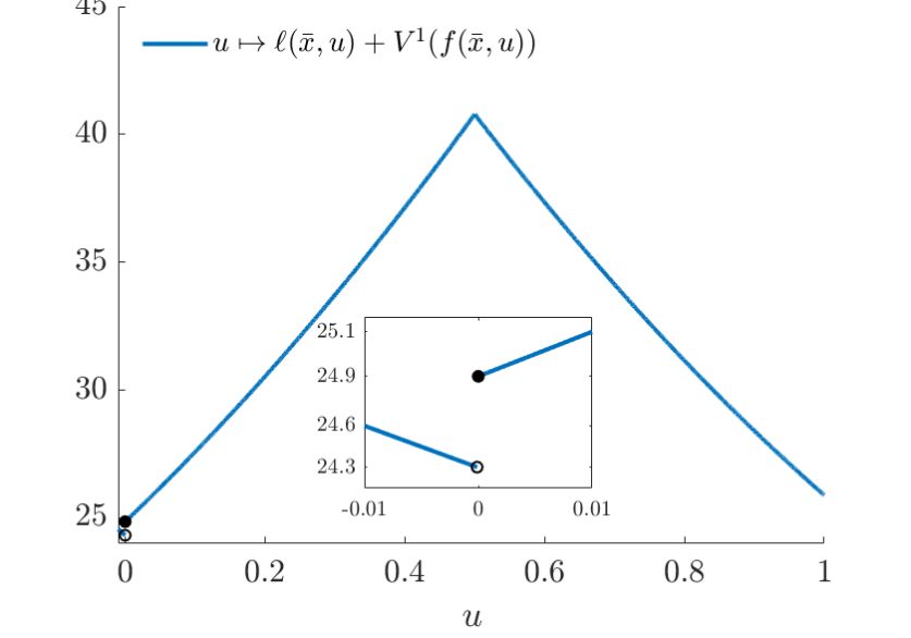
Figure 1: $u\mapsto\ell(\bar{x}+1,u)+V^{1}(f(\bar{x}+1,u))$ has no minimum.

4 Policy iteration plus

In this section we modify PI to enforce recursive feasibility under mild conditions, and we call the modified algorithm PI⁺. We show PI⁺ preserves the recursive (robust) stability and near-optimality properties stated for PI in Section 3.

4.1 The algorithm

PI⁺ is presented in 2. At any iteration $i\in\mathbb{Z}_{\geq 0}$, to enforce the existence of minimizer to $\ell(x,u)+V^{i}(f(x,u))$ over $u\in\mathcal{U}(x)$ in (PI.2) for any given $x\in\mathbb{R}^{n_{x}}$, we first regularize the set-valued map $H^{i+1}$ in (PI⁺.3), see [9, Def. 4.13]. For $x\in\mathbb{R}^{n_{x}}$, the set $H_{r}^{i+1}(x)$ is the intersection for all $\delta>0$ of the closures of sets $H^{i+1}(x+\delta\mathbb{B})$. As a result, $H_{r}^{i+1}$ in (PI⁺.3) is outer semicontinous [9, Lemma 5.16]. It is important to notice that $H^{i+1}(x)\subseteq H_{r}^{i+1}(x)$ for any $x\in\mathbb{R}^{n_{x}}$ and $i\in\mathbb{Z}_{\geq 0}$.

Algorithm 2 Policy Iteration Plus (PI⁺)

1:$f$ in (1), $\ell$ in (2), initial policy $h^{0}\in\mathcal{U}$

2:Policy $h_{r}^{\star,\infty}$, cost $V_{r}^{\infty}$

3:Initial evaluation step: for all $x\in\mathbb{R}^{n_{x}}$,

$$V_{r}^{0}(x):=J(x,h^{0}).$$ (PI⁺.1)

4:Let $H^{0}:=H_{r}^{0}:=H_{r}^{\star,0}:=\{h^{0}\}$.

5:for $i\in\mathbb{Z}_{\geq 0}$ do

6:   Policy improvement step: for all $x\in\mathbb{R}^{n_{x}}$,

$$H^{i+1}(x):=\operatorname*{\text{argmin}\,}\limits_{u\in\mathcal{U}(x)}\left\{\ell(x,u)+V_{r}^{i}(f(x,u))\right\}.$$ (PI⁺.2)

7:   Policy regularization step: for all $x\in\mathbb{R}^{n_{x}}$,

$$H_{r}^{i+1}(x):=\bigcap_{\delta>0}\overline{H^{i+1}(x+\delta\mathbb{B})}.$$ (PI⁺.3)

8:   Policy evaluation step: for all $x\in\mathbb{R}^{n_{x}}$,

$$V_{r}^{i+1}(x):=\min_{h_{r}^{i+1}\in H_{r}^{i+1}}J(x,h_{r}^{i+1}).$$ (PI⁺.4)

9:   Select $h_{r}^{\star,i+1}\in H_{r}^{\star,i+1}$ where, for all $x\in\mathbb{R}^{n_{x}}$,

$${\small H_{r}^{\star,i+1}(x){:=}\!\!\!\operatorname*{\text{argmin}\,}_{u\in H_{r}^{i+1}(x)}\!\!\!\!\!\!\left\{\ell(x,u)+V_{r}^{i+1}(f(x,u))\right\}\!.}$$ (PI⁺.5)

10:end for

11:return $h_{r}^{\star,\infty}\in H_{r}^{\star,\infty}$ and $V_{r}^{\infty}$.

The second modification compared to PI is on the evaluation step in (PI⁺.4). Given $i\in\mathbb{Z}_{\geq 0}$, for any $x\in\mathbb{R}^{n_{x}}$, instead of (PI.3), we define $V_{r}^{i+1}(x)$ as the minimum cost over all selections $h_{r}^{i+1}$ of $H_{r}^{i+1}$, see (PI⁺.4). Note that all selections do not necessarily lead to the same cost $V^{i+1}$, see Section 3.5 for an example. The differences with the evaluation step in PI are that we consider $H_{r}^{i+1}$, instead of $H^{i+1}$, and that we do not take an arbitrary selection of this set-valued map, but only those policies which give the minimum cost, see (PI⁺.5). Therefore, $V_{r}^{i+1}(\cdot)=J(\cdot,h_{r}^{\star,i+1})$ for any $h_{r}^{\star,i+1}\in H_{r}^{\star,i+1}$.

We will show that these two modifications are essential to ensure the recursive feasibility of PI⁺. It can also be already noted that, when $H^{i}$ is non-empty, outer semicontinuous and single-valued at any iteration $i\in\mathbb{Z}_{\geq 0}$, PI⁺ reduces to PI; we elaborate more on the links between PI and PI⁺ in Section 5.4.

Remark 5

Regarding the issue identified in the example of Section 3.5, PI⁺ produces cost $V^{1^{\prime}}$ and selects $h^{1^{\prime}}$ due (PI⁺.4) and (PI⁺.5), which ensures $u\mapsto\ell(\bar{x}+1,u)+V_{r}^{1}(f(\bar{x}+1,u))$ is lower semicontinuous for $u\in[-\delta,1]$ and thus $H^{2}(\bar{x}+1)$ is non-empty. $\Box$

Remark 6

In this work, we do not consider the possible errors arising from solving (PI⁺.3), (PI⁺.4) and (PI⁺.5) in practice. These relevant questions are left for future work. $\Box$

Remark 7

Lower semicontinuous regularizations of the optimal control problem is often considered in the literature for the optimal control of continuous-time systems, see, e.g., [8]. If we would consider a lower semicontinuous regularization of $(x,u)\mapsto\ell(x,u)+V^{i}(f(x,u))$ in (PI.2), instead of (PI⁺.3), to guarantee $H^{i+1}(x)$ is non-empty for any $x\in\mathbb{R}^{n_{x}}$, it is then unclear here whether: (i) $V^{\star}\leq V^{i+1}\leq V^{i}$; and (ii) that $V^{i+1}$ is the induced cost of some policy $h^{i+1}$. Both are key properties that allow for $V^{i}$ to converge to $V^{\star}$ when $i\to\infty$. $\Box$

4.2 Desired properties

Like in Section 3.2, the objectives in this section are to provide conditions under which PI⁺ is such that at any iteration $i\in\mathbb{Z}_{\geq 0}$:

• (recursive feasibility) for any $x\in\mathbb{R}^{n_{x}}$, $H^{i}(x)$, $H_{r}^{i}(x)$ and $H_{r}^{\star,i}(x)$ are non-empty;

• (recursive stability) system (1) whose inputs are generated by PI⁺, i.e.,

  $$x(k+1)\in f(x(k),H_{r}^{\star,i}(x(k)))=:F_{r}^{i}(x(k)),$$ (13)

  exhibits desirable set stability properties;

• (near-optimality guarantees) explicit bounds on $V_{r}^{i}(x)-V^{\star}(x)$ for any $x\in\mathbb{R}^{n_{x}}$ can be derived, which asymptotically go to zero as $i$ increases.

For convenience, we abuse notation to denote solutions to system (13) in the sequel as $\phi^{i}(\cdot,x)$ when initialized at some $x\in\mathbb{R}^{n_{x}}$ for any $i\in\mathbb{Z}_{\geq 0}$. As for PI, the robustness of the stability properties is deferred to Section 5.

4.3 Recursive feasibility

The recursive feasibility analysis rests on the next assumptions in addition to the ones from Section 3.3, which are all checkable a priori.

Assumption 2

The following holds.

1. The function $f$ and the stage cost function $\ell$ are continuous on $\mathbb{R}^{n_{x}}\times\mathbb{R}^{n_{u}}$.

2. $\ell$ is level-bounded in $u$, locally uniform in $x$.

3. $\mathcal{U}$ is outer semicontinuous on $\mathbb{R}^{n_{x}}$.

4. $V_{r}^{0}=J(x,h^{0})$ is lower semicontinuous on $\mathbb{R}^{n_{x}}$.

5. For all $\Delta>0$, the set $\{x\in\mathbb{R}^{n_{x}}:\sigma(x)\leq\Delta\}$ is compact. $\Box$

Item (i) of 2 imposes regularity conditions on model $f$ and stage cost $\ell$. Item (ii) of 2 is satisfied when $\ell(x,u)=\ell_{1}(x,u)+\ell_{2}(u)$ for any $(x,u)\in\mathbb{R}^{n_{x}}\times\mathbb{R}^{n_{u}}$ with $\ell_{1}(x,u)\geq 0$ and $\ell_{2}$ radially unbounded, i.e., $\ell_{2}(u)\to+\infty$ as $|u|\to+\infty$ for instance. A typical example of $\ell_{2}$ radially unbounded being $\ell_{2}(u)=u^{\top}Ru$ with $R\in\mathbb{R}^{n_{u}\times n_{u}}$ symmetric and positive definite; note that this property also trivially holds when $\mathcal{U}$ is independent of $x$ and compact. On the other hand, item (iii) of 2 is satisfied when $\mathcal{U}(\cdot)=\mathbb{R}^{n_{u}}$ or $\mathcal{U}(\cdot)$ is independent of $x$ and compact for example. Item (iv) of 2 is a mild regularity assumption on the initial cost function, which holds when $V_{r}^{0}$ is continuous on $\mathbb{R}^{n_{x}}$. Finally, item (v) of 2 implies $\sigma$ is radially unbounded, which implies that the attractor $\{x\in\mathbb{R}^{n_{x}}\,:\,\sigma(x)=0\}$ is compact.

Remark 8

The example in Section 3.5 verifies 1–3 and 2 with $\sigma(\cdot)=|\cdot|$, $W=\overline{\alpha}_{W}=0$, $\alpha_{W}=\chi_{W}=\mathbb{I}$ and $\overline{\alpha}_{V}=V_{r}^{0}\circ\sigma$ where $V_{r}^{0}=V^{0}$. As a consequence, the objectives stated for PI⁺ in Section 4.2 are satisfied for this example in view of the results presented next. $\Box$

The next theorem ensures recursive feasibility for PI⁺. For technical reasons, we prove recursive feasibility in conjunction with recursive stability for PI⁺ in Appendix 7.

Theorem 3

Suppose 2 holds. Sets $H^{i}(x)$, $H_{r}^{i}(x)$ and $H_{r}^{\star,i}(x)$ are non-empty for any $i\in\mathbb{Z}_{\geq 0}$ and $x\in\mathbb{R}^{n_{x}}$. $\Box$

Given the recursive feasibility of PI⁺ in 3, we now establish that the properties of PI in Section 3.4 also hold for PI⁺.

4.4 Recursive stability

The next theorem ensures recursive stability for PI⁺. Its proof is given in Appendix 7.

Theorem 4

Suppose 2 holds. For any $i\in\mathbb{Z}_{\geq 0}$, for any $x\in\mathbb{R}^{n_{x}}$, solution $\phi^{i}$ to (13) and $k\in\mathbb{Z}_{\geq 0}$,

$$\sigma(\phi^{i}(k,x))\leq\beta(\sigma(x),k)$$ (14)

where $\beta:(k,s)\mapsto\underline{\alpha}_{Y}^{-1}\circ(\mathbb{I}-\widetilde{\alpha}_{Y})^{(k)}\circ\overline{\alpha}_{Y}(s)\in\mathcal{KL}$ with $\underline{\alpha}_{Y},\overline{\alpha}_{Y},\widetilde{\alpha}_{Y}$ in Table 1. $\Box$

Similar to 1, 4 is a $\mathcal{KL}$-stability property of system (13) with respect to $\sigma$, with $\beta$ in (14). As previously mentioned, when $\sigma$ is a proper indicator of a compact set $\mathcal{A}$, (14) ensures that this set is uniformly globally asymptotically stable.

As in 1, when some of the functions in 1–3 satisfy stronger conditions, the stability property in 4 becomes exponential. A sketch of the proof is given in Section 7.8.

Corollary 2

Suppose 2 holds and that there exist $c_{W},a_{W},\overline{a}_{V}>0$ and $\overline{a}_{W}\geq 0$ such that $\chi_{W}(s)\leq c_{W}s$, $\alpha_{W}(s)\geq a_{W}s$, $\overline{\alpha}_{V}(s)\leq\overline{a}_{V}s$, $\overline{\alpha}_{W}(s)\leq\overline{a}_{W}s$ for any $s\geq 0$, where $\chi_{W},\alpha_{W},\overline{\alpha}_{W}$ come from 2 and $\overline{\alpha}_{V}$ comes from 3. Then, 4 holds with $\beta:(s,k)\mapsto\displaystyle\tfrac{\overline{a}_{Y}}{\underline{a}_{Y}}(1-\widetilde{a}_{Y})^{k}s\in{\exp}{-}\mathcal{KL}$, and $\widetilde{a}_{Y},\overline{a}_{Y},\underline{a}_{Y}$ in Table 1. $\Box$

4.5 Near-optimality properties

Similar to 2, the next theorem provides near-optimality guarantees for PI⁺. Its proof is given in the Section 8.1.

Theorem 5

Suppose 2 holds. For any $i\in\mathbb{Z}_{\geq 0}$ and $x\in\mathbb{R}^{n_{x}}$,

$$\begin{array}[]{rll}(V_{r}^{i}-V^{\star})(x)&\leq&(V_{r}^{0}-V^{\star})(\phi(i,x,h^{\star})),\end{array}$$ (15)

where $h^{\star}\in H^{\star}$ from (4). Moreover, for any $i\in\mathbb{Z}_{\geq 0}$ and $x\in\mathbb{R}^{n_{x}}$

$$\begin{array}[]{rll}V_{r}^{i}(x)-V^{\star}(x)\leq\widetilde{\alpha}\left(\beta(\sigma(x),i)\right),\end{array}$$ (16)

where $\beta\in\mathcal{KL}$ comes from 4 and $\widetilde{\alpha}=\max_{\hat{s}\in[0,s]}\widehat{\alpha}(\hat{s})$ is non-decreasing and positive definite function with $\widehat{\alpha}$ in Table 1. $\Box$

Similar to 2, 5 provides near-optimality guarantees to PI⁺. We conclude that $V_{r}^{i}\to V^{\star}$ as $i\to\infty$ point-wisely, as $\beta\in\mathcal{KL}$ and $\lim_{i\to\infty}\sigma(\phi(i,x,h^{\star}))=0$ by following similar lines as in the proof of 4. This qualitative property of PI⁺ is strengthened in (16) by employing a conservative bound for (15) in the form of $\widetilde{\alpha}\left(\beta(\sigma(x),i)\right)$, whose formulas for $\beta$ and $\widetilde{\alpha}$ are given in Theorems 4 and 5 in terms of functions in Table 1 and are thus known. Again, the fact that function $\beta$ in (14) is independent of the number of iterations $i$ ensures that the upper-bound converges to zero as $i$ increases to infinity.

Remark 9

As in 1, the bound in (16) can be used to design stopping criteria for PI⁺ to ensure a desired level of near-optimality. $\Box$

A direct consequence of 5 is that the sequence of cost functions $V_{r}^{i}$ converge compactly to $V^{\star}$, as formalized next.

Proposition 2

Suppose 2 holds. The sequence of functions $V_{r}^{i}$ monotonically compactly converges to $V^{\star}$, i.e.:

• for all $x\in\mathbb{R}^{n_{x}}$, $V_{r}^{i+1}(x)\leq V_{r}^{i}(x)$;

• for any compact set $K\subset\mathbb{R}^{n_{x}}$ and $\delta>0$ there exists $i^{\star}\in\mathbb{Z}_{>0}$ such that for any $x\in K$ and $i\geq i^{\star}$, $V_{r}^{i}(x)-V^{\star}(x)\leq\delta$ holds. $\mbox{}\hfill\Box$

2 establishes the uniform convergence of $V_{r}^{i}$ to $V^{\star}$ on any compact set $K\subset\mathbb{R}^{n_{x}}$, which, compared to 1, comes from the fact that level sets of $\sigma$ are compact in view of item (iv) of 2.

5 Robust stability

So far, we have established stability properties for system (1), whose inputs are generated either by PI or PI⁺. However, it is not clear yet whether these stability properties are robust to uncertainties and perturbations. Indeed, the corresponding closed-loop systems are given by difference inclusions and it has been shown in [12] in the context of model predictive control that difference inclusion may have zero robustness despite them satisfying so-called $\mathcal{KL}$-stability properties like in Theorems 1 and 4, in the sense that a vanishing arbitrarily small perturbation, may destroy asymptotic stability properties established for the unperturbed system. It is thus vital that the stability properties stated in Section 4.4 come with some nominal robustness properties. This is the focus of this section. The results are derived for system (13) controlled by PI⁺, but the same results follow when the inputs are generated by PI as explained in Section 5.4.

5.1 Nominal robustness definition

We consider the notion of nominal robustness in [21], which we recall below in the context of this paper. Let $\mathcal{X}\subseteq\mathbb{R}^{n_{x}}$ be open and such that $F_{r}^{i}(x)\subseteq\mathcal{X}$, where $F_{r}^{i}$ comes from (13), for any $x\in\mathcal{X}$ and $i\in\mathbb{Z}_{\geq 0}$. We introduce a continuous function $\rho:\mathcal{X}\to\mathbb{R}_{\geq 0}$ to perturb the set-valued map $F_{r}^{i}$ in (13) for $i\in\mathbb{Z}_{\geq 0}$ as

$$\begin{split}&F_{r,\rho}^{i}(x):=\\ &\!\!\!\!\!\left\{\eta\in\mathbb{R}^{n_{x}}:\eta\in\{\upsilon\}+\rho(\upsilon)\mathbb{B},\upsilon\in F_{r}^{i}(x+\rho(x)\mathbb{B})\!\right\}\!.\end{split}$$ (17)

We say that $F_{r,\rho}^{i}$ is the $\rho$-perturbation of $F_{r}^{i}$. Given $F_{r,\rho}^{i}$, we have the next difference inclusion

$$x(k+1)\in F_{r,\rho}^{i}(x(k)).$$ (18)

System (18) corresponds to system (13) perturbed by $\rho$, in the sense of (17). Note that $F_{r}^{i}=F_{r,\bm{0}}^{i}$ and $F_{r}^{i}\subseteq F_{r,\rho}^{i}$. We denote solutions to system (18) as $\phi^{i}_{\rho}(\cdot,x)$ when initialized at $x\in\mathbb{R}^{n_{x}}$ for $i\in\mathbb{Z}_{\geq 0}$.

4 establishes a $\mathcal{KL}{-}\text{stability}$ property with respect to $\sigma$ for which the attractor is $\mathcal{A}=\{x\in\mathbb{R}^{n_{x}}\,:\,\sigma(x)=0\}$ when $\sigma$ is a proper indicator of $\mathcal{A}$. To define robust stability as in [21], we consider instead a two-measure $\mathcal{KL}{-}\text{stability}$ property with respect to $(\sigma_{1},\sigma_{2})$ where $\sigma_{1},\sigma_{2}:\mathcal{X}\to\mathbb{R}_{\geq 0}$ are continuous. Given $\rho$ in (17), the attractor of perturbed system (18) becomes

$$\mathcal{A}^{i}_{\rho}:=\big{\{}\xi\in\mathcal{X}:\sup_{k\in\mathbb{Z}_{\geq 0}}\sigma_{1}(\phi^{i}_{\rho}(k,\xi))=0\big{\}}.$$ (19)

We are ready to define robust $\mathcal{KL}$-stability.

Definition 2 ([21])

Given $i\in\mathbb{Z}_{\geq 0}$ and $\sigma_{1},\sigma_{2}:\mathcal{X}\to\mathbb{R}_{\geq 0}$ continuous, system (13) is robustly $\mathcal{KL}$-stable with respect to $(\sigma_{1},\sigma_{2})$ on $\mathcal{X}$ if there exists a continuous function $\rho:\mathcal{X}\to\mathbb{R}_{\geq 0}$ such that the following holds.

• For all $x\in\mathcal{X}$, $\{x\}+\rho(x)\mathbb{B}\subset\mathcal{X}$.

• For all $x\in\mathcal{X}\setminus\mathcal{A}^{i}_{\bm{0}}$, $\rho(x)>0$.

• $\mathcal{A}^{i}_{\rho}=\mathcal{A}^{i}_{\bm{0}}$.

• System (18) is $\mathcal{KL}$-stable with respect to $(\sigma_{1},\sigma_{2})$ on $\mathcal{X}$, i.e., there exists $\beta\in\mathcal{KL}$ such that $\sigma_{1}(\phi^{i}_{\rho}(k,x))\leq\beta(\sigma_{2}(x),k)$ for every $x\in\mathcal{X}$ and $k\in\mathbb{Z}_{\geq 0}$. When $\sigma_{1}\,{=}\,\sigma_{2}\,{=}\,\sigma$, (13) is $\mathcal{KL}{-}\text{stable}$ with respect to $\sigma$. $\Box$

Item (i) of 2 imposes a condition on $\rho$ so that $F_{r,\rho}^{i}(\mathcal{X})\subseteq\mathcal{X}$ for any $i\in\mathbb{Z}_{\geq 0}$, as $F_{r}^{i}(x)\subseteq\mathcal{X}$ for all $x\in\mathcal{X}$. Item (ii) of 2 in turn requires that $\rho$ is non-zero outside the attractor $\mathcal{A}^{i}_{\bm{0}}$ corresponding to (19) with $\rho=0$. Then, item (iii) of 2 states that the perturbed attractor $\mathcal{A}^{i}_{\rho}$ is the same as the unperturbed one $\mathcal{A}^{i}_{\bm{0}}$. Finally, item (iv) of 2 says that the perturbed system is $\mathcal{KL}{-}\text{stable}$ with respect to $(\sigma_{1},\sigma_{2})$.

As advocated in [12], if a difference inclusion is $\mathcal{KL}{-}\text{stable}$ with respect to some measures $(\sigma_{1},\sigma_{2})$, it is not necessarily robustly $\mathcal{KL}{-}\text{stable}$. In other words, the (unperturbed) system may have zero robustness. In the context of this paper, sufficient conditions to conclude robust $\mathcal{KL}{-}\text{stability}$ with respect to some pair $(\sigma_{1},\sigma_{2})$ on $\mathcal{X}$ for system (13) with $i\in\mathbb{Z}_{\geq 0}$ are that:

• $F_{r}^{i}(x)$ is non-empty and compact for any $x\in\mathcal{X}$;

• the Lyapunov function used to establish the stability of the unperturbed system is continuous.

The next lemma states that item (a) above holds.

Lemma 1

Suppose 2 holds. For any $i\in\mathbb{Z}_{\geq 0}$, $F_{r}^{i}(x)$ is compact and non-empty for any $x\in\mathbb{R}^{n_{x}}$. $\Box$

Proof: Let $i\in\mathbb{Z}_{\geq 0}$ and $x\in\mathbb{R}^{n_{x}}$, since $f$ is continuous by item (i) of 2, the compactness of $F_{r}^{i}(x)=f\left(x,H_{r}^{\star,i}(x)\right)$ follows from the compactness of $H_{r}^{\star,i}$, which we now show. To this end, we prove that the conditions of [27, Theorem 1.17(a)] are verified by invoking similar arguments to those employed in the proof of 4 in Section 7.5. Consider $g_{r}^{i}:(x,u)\mapsto\ell(x,u)+V_{r}^{i}(f(x,u))+\delta_{H_{r}^{i}(x)}(u)$. On the one hand, $g_{r}^{i}$ is proper and level-bounded in $u$, locally uniform in $x$, for the same reasons as stated in the proof of 4. On the other hand, $(x,u)\mapsto\ell(x,u)+V_{r}^{i}(f(x,u))$ is lower semicontinuous on $\mathbb{R}^{n_{x}}\times\mathbb{R}^{n_{u}}$, in view of the lower semicontinuity of $V_{r}^{i}$ on $\mathbb{R}^{n_{x}}$ from 9 in Appendix 7 and the continuity of $f$ and $\ell$ by 2. Moreover, $\delta_{H_{r}^{i}(\cdot)}(\cdot)$ is lower semicontinuous on $\mathbb{R}^{n_{x}}\times\mathbb{R}^{n_{u}}$, as this holds from 12 in Section 11 since $H_{r}^{i}$ is an outer semicontinuous set-valued in view of [9, Lemma 5.16]. Thus $g_{r}^{i}$ is lower semicontinuous on $\mathbb{R}^{n_{x}}\times\mathbb{R}^{n_{u}}$ and all the conditions of [27, Theorem 1.17(a)] hold, we can therefore apply it to conclude $H_{r}^{\star,i+1}(x)$ in (PI⁺.2) is non-empty and compact at $x\in\mathbb{R}^{n_{x}}$. Since $x$ has been selected arbitrarily, the desired result follows. $\mbox{}\hfill\blacksquare$

Regarding item (b), it turns out that the Lyapunov function used to establish $\mathcal{KL}{-}\text{stability}$ in Section 4.4, namely $Y^{i}=\rho_{V}(V_{r}^{i})+\rho_{W}(W)$, is only guaranteed to be lower semicontinuous. Indeed, while $W,\rho_{V}$ and $\rho_{W}$ are continuous, $V_{r}^{i}$ is only shown to be lower semicontinuous in 9 given in Appendix 7. Thus we will require a different analysis or extra assumptions as presented next.

5.2 Robust semi-global practical stability

An alternative Lyapunov function to analyse the stability of (13) is $Y^{\star}:=\rho_{V}(V^{\star})+\rho_{W}(W)$, where $V^{\star}$ is the optimal value function defined in (3), which is known to be continuous in view of [26, Theorem 3] under a mild additional assumption on $\mathcal{U}$ that can be checked a priori.

Assumption 3

Set-valued map $\mathcal{U}$ is continuous and locally bounded on $\mathbb{R}^{n_{x}}$. $\Box$

However, function $Y^{\star}$ only allows to establish a semiglobal practical $\mathcal{KL}{-}\text{stability}$ property under SA1–3 for $i$ is sufficiently large so that, somehow, $V_{r}^{i}$ is sufficiently close to $V^{\star}$ in view of 2. The next theorem provides a first robustness guarantee for the stability property established in 4. Its proof is given in Section 10.1.

Theorem 6

For any $\delta,\Delta>0$, let $\sigma_{1}=\max\{\sigma-\delta,0\}$, $\sigma_{2}=\sigma$, $\mathcal{X}=\{x\in\mathbb{R}^{n_{x}}\,:\,\sigma(x)<\Delta\}$ and suppose Assumptions 2 and 3 hold. There exists $i^{\star}\in\mathbb{Z}_{\geq 0}$ such that, for any $i\geq i^{\star}$, system (13) is robustly $\mathcal{KL}{-}\text{stable}$ with respect to $(\sigma_{1},\sigma_{2})$ on $\mathcal{X}$. $\Box$

6 implies that the stability property of system (13) established in 4 is robust in a semiglobal practical sense after sufficiently many iterations $i$ with $i\geq i^{\star}$ and $i^{\star}$ depends on $\delta,\Delta$. It is a semiglobal property as we consider the set of initial conditions as $\{x\in\mathbb{R}^{n_{x}}\,:\,\sigma(x)<\Delta\}$ instead of $\mathbb{R}^{n_{x}}$, and it is practical as $\sigma_{1}$ is given by $\max\{\sigma(\cdot)-\delta,0\}$ instead of $\sigma$.

By strengthening the assumptions given in Section 3.3, we can ensure stronger robustness guarantees as shown in the next corollaries.

Corollary 3

For any $\Delta>0$, let $\mathcal{X}=\{x\in\mathbb{R}^{n_{x}}\,:\,\sigma(x)<\Delta\}$ and suppose Assumptions 2 and 3 hold. There exists $i^{\star}\in\mathbb{Z}_{\geq 0}$ such that, for any $i\geq i^{\star}$, system (13) is robustly $\mathcal{KL}{-}\text{stable}$ with respect to $\sigma$ on $\mathcal{X}$ when there exist $l\in\mathbb{R}_{>0}$, $c_{W},a_{W},\overline{a}_{V}>0$ and $\overline{a}_{W},\widetilde{a}\geq 0$ such that, for any $s\in[0,l)$, $\chi_{W}(s)\leq c_{W}s$, $\alpha_{W}(s)\geq a_{W}s$, $\overline{\alpha}_{V}(s)\leq\overline{a}_{V}s$, $\overline{\alpha}_{W}(s)\leq\overline{a}_{W}s$, $\widetilde{\alpha}(s)\leq\widetilde{a}s$. $\Box$

3 extends 6 to allow $\delta=0$, thus enabling robust semiglobal asymptotic stability guarantees. The proof follows by the same manipulations as in the proofs of [11, Corollary 1] or [13, Corollary 2] and is thus omitted. The next corollary ensures a robust global practical stability property under different conditions.

Corollary 4

For any $\delta>0$, let $\sigma_{1}=\max\{\sigma(\cdot)-\delta,0\}$ and suppose Assumptions 2 and 3 hold. There exists $i^{\star}\in\mathbb{Z}_{\geq 0}$ such that, for any $i\geq i^{\star}$, system (13) is robustly $\mathcal{KL}{-}\text{stable}$ with respect to $(\sigma_{1},\sigma)$ on $\mathcal{X}=\mathbb{R}^{n_{x}}$ when there exist $L\in\mathbb{R}_{\geq 0}$, $c_{W},a_{W},\overline{a}_{V}>0$ and $\overline{a}_{W},\widetilde{a}\geq 0$ such that, for any $s\in[L,\infty)$, $\chi_{W}(s)\leq c_{W}s$, $\alpha_{W}(s)\geq a_{W}s$, $\overline{\alpha}_{V}(s)\leq\overline{a}_{V}s$, $\overline{\alpha}_{W}(s)\leq\overline{a}_{W}s$, $\widetilde{\alpha}(s)\leq\widetilde{a}s$. $\Box$

4 extends 6 to allow $\Delta=\infty$, thus indeed enabling for robust global practical stability guarantees. The proof also follows by similar manipulations as in the proofs of [11, Corollary 1] or [13, Corollary 2] and is thus omitted. Finally, we can combine the conditions of Corollaries 3 and 4 to provide robust global and asymptotic stability properties. Its proof is omitted as it follows from 6, Corollaries 3 and 4.

Corollary 5

Suppose Assumptions 2 and 3 hold. There exists $i^{\star}\in\mathbb{Z}_{\geq 0}$ such that, for any $i\geq i^{\star}$, system (13) is robustly $\mathcal{KL}{-}\text{stable}$ with respect to $\sigma$ on $\mathcal{X}=\mathbb{R}^{n_{x}}$ when both conditions at the end of Corollaries 3 and 4 are satisfied. $\Box$

The results of this section establishes robust stability properties only when sufficiently many iterations of PI⁺ have been performed. When $V_{r}^{0}$ is sufficiently close to $V^{\star}$, the required number of iterations for robust stability may be as low as 0. In general, however, we might not have robust stability at the first iterations. In order to establish robustness of the global asymptotic stability of PI⁺ at any iteration, we require extra assumptions, which are presented in the next section.

5.3 Robust global asymptotic stability

It is possible to ensure robust stability at any iteration by adding an assumption on the problem, thanks to which $V_{r}^{i}$ can be shown to be continuous so that the desired robustness property follows from [21].

Assumption 4

For any iteration $i\in\mathbb{Z}_{\geq 0}$, for any two selections $h,h^{\prime}\in H^{i}$, $J(\cdot,h)=J(\cdot,h^{\prime})$. $\Box$

4 implies that all selections at any given iteration have the same induced cost. This arises, for example, when $H^{i}$ is single-valued at any $i\in\mathbb{Z}_{\geq 0}$, which for instance occurs when the plant dynamics is linear and the cost is quadratic under mild conditions. While verifying 4 a priori is not trivial, we can check this condition at each iteration for certain classes of optimal control problems, e.g., when the set of different selections of $H^{i}$ is finite.

We establish the next key result that follows from 4, whose proof is given in Section 10.2.

Proposition 3

Suppose Assumptions 2 and 4 hold and $h^{0}\in\mathcal{U}$ be such that $J(\cdot,h^{0})$ is continuous. Then, for any $i\in\mathbb{Z}_{\geq 0}$, $V_{r}^{i}$ is continuous on $\mathbb{R}^{n_{x}}$. $\Box$

3 gives a condition for $V_{r}^{i}$ to be continuous.

Remark 10

While 3 is vital for the subsequent robustness analysis, its consequences are interesting in their own right. Indeed, knowing that $V_{r}^{i}$ is continuous is useful when $f$ is unknown, which is not the case in this paper, as it allows using a variety of techniques to learn the value function and an associated policy at each iteration on any given compact set. $\Box$

We provide the next robustness analysis for PI⁺ under 4. The proof is given in Section 10.3.

Theorem 7

Suppose Assumptions 2 and 4 hold and $h^{0}\in\mathcal{U}$ be such that $J(\cdot,h^{0})$ is continuous. Then, for any $i\in\mathbb{Z}_{\geq 0}$ system (13) is robustly $\mathcal{KL}{-}\text{stable}$ with respect to measure $\sigma$ on $\mathcal{X}=\mathbb{R}^{n_{x}}$ for any $i\in\mathbb{Z}_{\geq 0}$. $\Box$

In contrast to 6, 7 shows that the stability guarantee given by 4 is indeed robust at any iteration.

5.4 Robustness for PI

The robustness properties established for PI⁺ also apply to PI. Indeed, when $F^{i}$ is compact and non-empty on $\mathbb{R}^{n_{x}}$ for every $i\in\mathbb{Z}_{\geq 0}$, we can draw corresponding robustness guarantees for PI. In turn, $F^{i}$ compact and non-empty on $\mathbb{R}^{n_{x}}$ for every $i\in\mathbb{Z}_{\geq 0}$ holds when 2 holds and $V^{i}$ is lower semicontinuous for every $i\in\mathbb{Z}_{\geq 0}$.

Moreover, PI⁺ reduces to PI under 4 is satisfied, i.e., $V_{r}^{i}=V^{i}$ when $V_{r}^{0}=V^{0}$ and continuous. To see this, note that $V_{r}^{0}$ continuous implies that $H^{1}$ is outer semicontinuous, hence $H^{1}=H_{r}^{1}$. Then, 4 guarantees that any selection of $H^{1}_{r}$ produces the same induced cost, hence $H^{1}_{r}=H^{\star,1}_{r}$. Thus $H^{\star,1}_{r}=H^{1}$ and $V_{r}^{1}=V^{1}$, which are also continuous in view of 3 for $i=1$. The above reasoning allows to obtain $V_{r}^{i}=V^{i}$ holds for any $i\in\mathbb{Z}_{\geq 0}$ by induction. In conclusion, we also endow classical PI with robustness guarantees as in Section 5.3 when 4 holds.

6 Conclusion

We presented conditions to ensure recursive robust set stability properties for deterministic nonlinear discrete-time systems whose inputs are generated by PI. We also gave novel near-optimality properties, which do not rely on a discount factor contrary to the related works of the literature, see, e.g., [2, 4]. Because PI may fail to be recursively feasible, we have then modified it to address this issue, which leads to the algorithm called PI⁺. PI⁺ was shown to be recursively feasible under mild conditions and to preserve the robust stability and near-optimality properties of PI when the attractor is compact. It will be interesting in future work to study the conservatism of the given near-optimality bounds and to extend the current robustness properties to address more general non-vanishing perturbations, possibly in a data-driven case, as recently done in [25] for linear systems.

7 Proofs of Theorems 3 and 4

7.1 Proof outline

We prove Theorems 3 and 4 together by invoking the next proposition.

Proposition 4

For all $i\in\mathbb{Z}_{\geq 0}$, the following holds.

• For any $x\in\mathbb{R}^{n_{x}}$, $H^{i}(x)$, $H_{r}^{i}(x)$ and $H_{r}^{\star,i}(x)$ are non-empty.

• For any $x\in\mathbb{R}^{n_{x}}$ and $k\in\mathbb{Z}_{\geq 0}$, $\sigma(\phi^{i}(k,x))\leq\beta(\sigma(x),k)$ holds with $\beta\in\mathcal{KL}$ in 4.

• For any $h_{r}^{\star,i}\in H_{r}^{\star,i}$ and $x\in\mathbb{R}^{n_{x}}$, $V_{r}^{i}(x)=J(x,h_{r}^{\star,i}(x))\leq\overline{\alpha}_{V}(\sigma(x))$.

• $V_{r}^{i}$ is lower semicontinuous on $\mathbb{R}^{n_{x}}$. $\Box$

Item (i) of 4 corresponds to 3, item (ii) of 4 in turn corresponds to 4, while items (iii) and (iv) of 4 are technical properties used in the proof of 4.

4 is proved by induction in this appendix. We first analyse the base case, i.e., $i=0$. We establish items (i)-(iv) 4 for $i=0$ by virtue of 2–3 and 2, (PI⁺.1) and Line 4 of 2. In particular, for $i=0$, items (i), (iii) and (iv) of 4 follow immediately from 3, 2 and 2, while item (ii) of 4 is a consequence of 2 and 3. Afterwards, we will proceed with the induction step, namely we consider $i\in\mathbb{Z}_{\geq 0}$ and we assume that (i)-(iv) of 4 hold for $i$, we then show that they also hold for $i+1$. We proceed in steps. First feasibility of the improvement step is proved, in the sense that $H^{i+1}(x)$ and $H^{i+1}_{r}(x)$ are non-empty for any $x\in\mathbb{R}^{n_{x}}$, and we also show $H^{i+1}$ in (PI⁺.2) and $H_{r}^{i+1}$ in (PI⁺.3) are locally bounded on $\mathbb{R}^{n_{x}}$ by virtue of the inductive hypothesis. Next, we study the feasibility of the evaluation step, and show that $V_{r}^{i+1}$ in (PI⁺.4) is well defined and is upper-bounded by $V_{r}^{i}$, hence by $\overline{\alpha}_{V}\circ\sigma$. This in turn allows us to provide stability guarantees for system (13) for $i+1$, which is given by (1) in closed-loop with $H_{r}^{\star,i+1}$ from (PI⁺.5). As a consequence, we prove that $V_{r}^{i+1}$ is lower semicontinuous, and conclude that items (i)-(iv) of 4 hold for $i+1$ thereby completing the proof.

7.2 Proof of 4

We first verify the base case, which is that items (i)-(iv) of 4 hold for $i=0$, and we then address the induction step.

7.2.1 Base case $(i=0)$

In view of 3, item (iv) of 2, (PI⁺.1) and Line 4 of 2, we have that items (i), (iii) and (iv) of 4 hold for $i=0$.

We now show that item (ii) of 4 holds for $i=0$. For this purpose, we establish in the next lemma the existence of a strict Lyapunov function for system (13) for $i=0$, whose proof is given in Section 7.3.

Lemma 2

There exist $\underline{\alpha}_{Y},\overline{\alpha}_{Y},\alpha_{Y},\rho_{V},\rho_{W}\in\mathcal{K}_{\infty}$ such that $Y^{0}:=\rho_{V}(V_{r}^{0})+\rho_{W}(W)$ satisfies

$$\begin{split}\underline{\alpha}_{Y}(\sigma(x))\leq Y^{0}(x)&{}\leq\overline{\alpha}_{Y}(\sigma(x))\\ Y^{0}(\upsilon)-Y^{0}(x)&{}\leq-\alpha_{Y}(\sigma(x))\end{split}$$ (20)

for any $x\in\mathbb{R}^{n_{x}}$ and $v\in F_{r}^{0}(x)$. $\Box$

The next lemma formalizes the uniform global asymptotic stability property for system (13) at iteration $i=0$ based on 2. Its proof is given in Section 7.4.

Lemma 3

For any $x\in\mathbb{R}^{n_{x}}$, the corresponding solution $\phi^{0}$ to (13) for $i=0$ verifies $\sigma(\phi^{0}(k,x))\leq\beta(\sigma(x),k)$ with $\beta\in\mathcal{KL}$ in 4. $\Box$

As item (ii) of 4 holds for $i=0$ in view of 3, we have proved that 4 holds at $i=0$. It is important for the following to note that $\beta$ is constructed in terms of $\overline{\alpha}_{V},\overline{\alpha}_{W},\chi_{W}$ and $\alpha_{W}$, so that we can establish later that $\beta$ is independent of $i$.

7.2.2 Induction step $(``i\Rightarrow i+1")$

We now proceed to the induction step, and assume 4 holds for $i\in\mathbb{Z}_{\geq 0}$.

Inductive Hypothesis (IH)

Items (i)-(iv) of 4 hold for $i$. $\Box$

Under Section 7.2.2, we show items (i)-(iv) of 4 holds for $i+1$.

Feasibility of the improvement step: The following lemma ensures that $H^{i+1}$ in (PI⁺.2) and $H_{r}^{i+1}$ in (PI⁺.3) are non-empty and locally bounded on $\mathbb{R}^{n_{x}}$. Its proof is given in Section 7.5.

Lemma 4

Set-valued maps $H^{i+1}$ in (PI⁺.2) and $H_{r}^{i+1}$ in (PI⁺.3) are non-empty and locally bounded on $\mathbb{R}^{n_{x}}$. $\Box$

We now seek to evaluate $V_{r}^{i+1}$.

Feasibility of the evaluation step: For the $(i+1)^{\text{th}}$ evaluation step of PI⁺ in (PI⁺.4), we need to show that the minimum cost over any selection of $H_{r}^{i+1}$ is well-defined. In other words, that $H_{r}^{\star,i+1}(x)$ in (PI⁺.5) is non-empty for any $x\in\mathbb{R}^{n_{x}}$. For the sake of convenience, we extend the state vector as $\chi:=(x,u)\in\mathbb{R}^{n_{x}}\times\mathbb{R}^{n_{u}}$ and we write

$$\chi(k+1)\in\big{(}f(x,u),H_{r}^{i+1}\big{(}f(x,u)\big{)}\big{)}=:G^{i+1}(\chi(k)).$$ (21)

Given any $x\in\mathbb{R}^{n_{x}}$, we consider initial conditions to (21) of the form $(x,u)$ with $u\in H_{r}^{i+1}(x)$ with $H_{r}^{i+1}$ defined in (PI⁺.3), and we denote the associated set of solutions to (21) by $\mathcal{S}^{i+1}(x)$, which only depends on $x$. To extend the state vector as in (21) allows to write the stage cost as a function of $\chi$ only, i.e., $\ell(x,u)=\ell(\chi)$, which is convenient in the sequel. We now evaluate the cost of solutions to (21), that is, in view of (PI⁺.4), for any $x\in\mathbb{R}^{n_{x}}$,

$$V_{r}^{i+1}(x)=\min_{\psi^{i+1}\in\mathcal{S}^{i+1}(x)}\sum_{k=0}^{\infty}\ell\big{(}\psi^{i+1}(k,x)\big{)},$$ (22)

where $\psi^{i+1}=(\phi^{i+1},v^{i+1})\in\mathcal{S}^{i+1}(x)$ is a solution to system (21) initialized at $(x,h_{r}^{i+1}(x))$ with $h_{r}^{i+1}(x)\in H_{r}^{i+1}(x)$. To guarantee the existence of a minimum in (22), we invoke similar arguments as in [20, Claim 24]. For this purpose, we first state the next properties of $G^{i+1}$ in (21).

Lemma 5

Function $G^{i+1}$ in (21) is outer semicontinuous, locally bounded on $\mathbb{R}^{n_{x}}\times\mathbb{R}^{n_{u}}$ and $G^{i+1}(\chi)$ is non-empty for any $\chi\in\mathcal{W}^{i+1}:=\{(x,u)\in\mathbb{R}^{n_{x}}\times\mathbb{R}^{n_{u}}\,:u\in H_{r}^{i+1}(x)\}$. $\Box$

Proof: Since single-valued $f$ is continuous on $\mathbb{R}^{n_{x}}\times\mathbb{R}^{n_{u}}$ by item (i) of 2, it is locally bounded and outer-semicontinuous on $\mathbb{R}^{n_{x}}\times\mathbb{R}^{n_{u}}$ by [27, Corollary 5.20]. Moreover, as $H_{r}^{i+1}$ in (PI⁺.3) is locally bounded by 4 and outer semicontinuous on $\mathbb{R}^{n_{x}}$ by [9, Lemma 5.16], we deduce that $G^{i+1}$ is locally bounded and outer semicontinuous on $\mathbb{R}^{n_{x}}\times\mathbb{R}^{n_{u}}$ by [27, Proposition 5.52(a) and (b)]. Finally, $G^{i+1}(\chi)$ is non-empty for any $\chi\in\mathcal{W}^{i+1}$ as $H_{r}^{i+1}(x)$ is non-empty for $x\in\mathbb{R}^{n_{x}}$ by 4. $\blacksquare$

We verify the existence of a policy as in (PI⁺.5) for $i+1$, and we provide key properties of such policy in the next proposition, whose proof is in Section 7.6.

Lemma 6

There exists $h_{r}^{\star,i+1}\in H_{r}^{\star,i+1}$ such that $V_{r}^{i+1}(x)=J(x,h_{r}^{\star,i+1})$ for all $x\in\mathbb{R}^{n_{x}}$. Furthermore, the following holds for any $x\in\mathbb{R}^{n_{x}}$,

1. $V_{r}^{i+1}(x)=\ell(x,h_{r}^{\star,i+1}(x))+V_{r}^{i+1}\big{(}f(x,h_{r}^{\star,i+1}(x))\big{)}$,

2. $V_{r}^{i+1}(x)\leq V_{r}^{i}(x)\leq\overline{\alpha}_{V}(\sigma(x))$. $\Box$

In view of Lemmas 4 and 6, items (i) and (iii) of 4 are verified at $i+1$. We now establish stability properties as in item (ii) of 4 at $i+1$, which then allows to show the lower semicontinuity of $V_{r}^{i+1}$, which is the final item (iv) of 4.

Stability: We follow similar lines as in Section 7.2.1 to analyze the stability of system (13) at iteration $i+1$. The next result establish the existence of a strict Lyapunov function for the $(i+1)^{\text{th}}$-step of PI⁺, similar to the one found in 2. The proof relies on similar arguments as the proof of 2 in Section 7.3, and is hence omitted.

Lemma 7

For any $x\in\mathbb{R}^{n_{x}}$ and $v\in F_{r}^{i+1}(x)$,

$$\begin{split}\underline{\alpha}_{Y}(\sigma(x))\leq Y^{i+1}(x)&{}\leq\overline{\alpha}_{Y}(\sigma(x))\\ Y^{i+1}(\upsilon)-Y^{i+1}(x)&{}\leq-\alpha_{Y}(\sigma(x))\end{split}$$ (23)

with $Y^{i+1}:=\rho_{V}(V_{r}^{i+1})+\rho_{W}(W)$ and $\underline{\alpha}_{Y},\allowbreak\overline{\alpha}_{Y},\allowbreak\alpha_{Y},\allowbreak\rho_{V},\allowbreak\rho_{W}\in\mathcal{K}_{\infty}$ as in 2. $\Box$

The next result follows from 7. Its proof is very similar to the proof of 3 in Section 7.4, it is therefore omitted.

Lemma 8

For any $x\in\mathbb{R}^{n_{x}}$, any solution $\phi^{i+1}$ to (13) verifies $\sigma(\phi^{i+1}(k,x))\leq\beta(\sigma(x),k)$ with $\beta\in\mathcal{KL}$ in 4. $\Box$

Since, in 3, we have $\beta$ only constructed in terms of $\overline{\alpha}_{V},\overline{\alpha}_{W},\chi_{W}$ and $\alpha_{W}$, we therefore obtain $\beta$ independent of $i+1$ in 8. This establishes item (ii) of 4 at $i+1$. All that remains to prove is item (iv) of 4 for $i+1$.

Lower semicontinuity of $V_{r}^{i+1}$: The next lemma establishes the lower semicontinuity of $V_{r}^{i+1}$, whose proof is given in Section 7.7 and is inspired by [20, Theorem 6].

Lemma 9

$V_{r}^{i+1}$ is lower semicontinuous on $\mathbb{R}^{n_{x}}$. $\Box$

We have obtained lower semicontinuous $V_{r}^{i+1}$ and items (i)-(iv) of 4 holds for $i+1$. Therefore 4 holds for $i+1$ and the induction proof of 4 is complete. We then deduce that Theorems 3 and 4 hold.

The remaining part of Appendix 7 is dedicated to the proofs of the various lemmas stated above to prove 4.

7.3 Proof of 2

The proof follows similar lines as the proofs of [13, Theorem 1] and [26, Theorem 1]. We distinguish two cases.

Case where $\bm{\chi_{W}\leq\mathbb{I}}$: Let $\rho_{V}:=\rho_{W}:=\mathbb{I}$, thus $Y^{0}=\rho_{V}(V_{r}^{0})+\rho_{W}(W)=V_{r}^{0}+W$. By 2 and 3, $Y^{0}(x)\leq\overline{\alpha}_{V}(\sigma(x))+\overline{\alpha}_{W}(\sigma(x))$ for any $x\in\mathbb{R}^{n_{x}}$, therefore $\overline{\alpha}_{Y}:=\overline{\alpha}_{V}+\overline{\alpha}_{W}$. On the other hand, by 2 and since $\chi_{W}\leq\mathbb{I}$, $\alpha_{W}(\sigma(x))\leq\ell(x,u)+W(x)$ for any $(x,u)\in\mathcal{W}$, hence $Y^{0}(x)=V_{r}^{0}(x)+W(x)\geq\ell(x,h^{0}(x))+W(x)\geq\alpha_{W}(\sigma(x))$, therefore $\underline{\alpha}_{Y}:=\alpha_{W}$. Moreover, since $V_{r}^{0}(x)=J(x,h^{0})=\ell(x,h^{0}(x))+J(f(x,h^{0}(x)),h^{0})=\ell(x,h^{0}(x))+V_{r}^{0}(f(x,h^{0}(x)))$, we have for $\upsilon=f(x,h^{0}(x))$ that

$$V_{r}^{0}(\upsilon)-V^{0}(x)=-\ell(x,h^{0}(x)).$$ (24)

Again by 2 as $\chi_{W}\leq\mathbb{I}$ and $u=h^{0}(x)$,

$$W(\upsilon)-W(x)\leq-\alpha_{W}(\sigma(x))+\ell(x,u).$$ (25)

Summing (24) and (25), we obtain $Y^{0}(\upsilon)-Y(x)\leq-\alpha_{W}(\sigma(x))$, therefore $\alpha_{Y}:=\alpha_{W}$. The case is complete.

Case where $\bm{\chi(s)>s}$ for some $\bm{s>0}$: We define $q_{V}:=\displaystyle 2\chi_{W}(2\mathbb{I})$ and $q_{W}:=\frac{1}{2}[\chi_{W}+(\overline{\alpha}_{W}+\mathbb{I})\circ\alpha_{W}^{-1}(2\chi_{W})]^{-1}$, where the involved functions come from 2. Note that $q_{W}$ is well-defined as $\chi_{W}+(\overline{\alpha}_{W}+\mathbb{I})\circ\alpha_{W}^{-1}(2\chi_{W})$ is invertible, being a class-$\mathcal{K}_{\infty}$ function. Moreover, both $q_{V}$ and $q_{W}$ are of class-$\mathcal{K}_{\infty}$. We further define $\rho_{V}(s):=\int_{0}^{s}q_{V}(\tau)d\tau$ and $\rho_{W}(s):=\int_{0}^{s}q_{W}(\tau)d\tau$ for any $s\geq 0$. Note that $\rho_{V}$ and $\rho_{W}$ are also of class-$\mathcal{K}_{\infty}$. We are ready to define the Lyapunov function used to prove stability.

Let $x\in\mathbb{R}^{n_{x}}$ and $v\in F_{r}^{0}(x)$. According to 2 and 3, $Y^{0}(x)\leq\rho_{V}\circ\overline{\alpha}_{V}(\sigma(x))+\rho_{W}\circ\overline{\alpha}_{W}(\sigma(x))=:\overline{\alpha}_{Y}(\sigma(x))$ and $\overline{\alpha}_{Y}$ is of class-$\mathcal{K}_{\infty}$ in view of the properties of the functions $\rho_{V},\rho_{W},\overline{\alpha}_{V}$ and $\overline{\alpha}_{W}$. On the other hand, from (24), for any $x\in\mathbb{R}^{n_{x}}$,

$$V_{r}^{0}(x)\geq\ell(x,h^{0}(x))$$ (26)

and in view of 2, $Y^{0}(x)\geq\rho_{V}(\ell(x,h^{0}(x)))+\rho_{W}\left(\max\left\{\alpha_{W}(\sigma(x))-\chi_{W}(\ell(x,h^{0}(x)))),0\right\}\right)$. When $\frac{1}{2}\alpha_{W}(\sigma(x))\leq\chi_{W}(\ell(x,h^{0}(x)))$, it follows $Y^{0}(x)\geq\rho_{V}\circ\chi_{W}^{-1}(\frac{1}{2}\alpha_{W}(\sigma(x)))$. When $\frac{1}{2}\alpha_{W}(\sigma(x))\geq\chi_{W}(\ell(x,h^{0}(x))))$ then $Y^{0}(x)\geq\rho_{W}\circ\frac{1}{2}\alpha_{W}(\sigma(x))$. Hence $Y^{0}(x)\geq\underline{\alpha}_{Y}(\sigma(x))$ with $\underline{\alpha}_{Y}:=\min\left\{\rho_{V}\circ\chi_{W}^{-1}(\frac{1}{2}\alpha_{W}),\rho_{W}(\frac{1}{2}\alpha_{W})\right\}\in\mathcal{K}_{\infty}$. We have proved the first line in (20).

In view of (24), (26) and 3, the conditions of [13, Lemma 3] are satisfied with $h(x)=\ell(x,h^{0}(x))$, $\alpha_{1}=\overline{\alpha}_{V}$ and $\alpha_{2}=0$. Thus, we derive that

$$\rho_{V}(V_{r}^{0}(v))-\rho_{V}(V_{r}^{0}(x))$$

$$\leq-\chi_{W}(\ell(x,h^{0}(x)))\ell(x,h^{0}(x))).$$ (27)

On the other hand, the conditions of [13, Lemma 4] are verified with $\alpha_{1}=\overline{\alpha}_{W}+\mathbb{I}$, $\alpha_{2}=\chi_{W}$ and $\alpha_{3}=\alpha_{W}$, according to 2. Hence, we deduce from [13, Lemma 4]

$$\rho_{W}(W(v))-\rho_{W}(W(x))$$

$$\!\!\!\!\!\!\!\!{}\leq 2q_{W}\Big{(}\chi_{W}(\ell(x,h^{0}(x)))+\alpha_{1}\circ\alpha_{W}^{-1}(2\chi_{W}(\ell(x,h^{0}(x))))\Big{)}$$

$$\!\!\!\!\!\!\!\!\qquad\times\chi_{W}(\ell(x,h^{0}(x)))-q_{W}(\tfrac{1}{4}\alpha_{W}(\sigma(x)))\tfrac{1}{4}\alpha_{W}(\sigma(x))$$

$$\!\!\!\!\!\!\!\!{}=\ell(x,h^{0}(x))\chi_{W}(\ell(x,h^{0}(x)))-\widetilde{\alpha}_{W}(\sigma(x))$$ (28)

where $\widetilde{\alpha}_{W}=q_{W}(\frac{1}{4}\alpha_{W})\frac{1}{4}\alpha_{W}\in\mathcal{K}_{\infty}$. In view of (27) and (28), it follows that $Y^{0}(v)-Y^{0}(x)\leq-\chi_{W}(\ell(x,h^{0}(x)))\allowbreak\ell(x,h^{0}(x)))+\ell(x,h^{0}(x))\chi_{W}(\ell(x,h^{0}(x)))-\widetilde{\alpha}_{W}(\sigma(x))\leq-\widetilde{\alpha}_{W}(\sigma(x))$. We have shown that the second line in (20) holds with $\alpha_{Y}=\widetilde{\alpha}_{W}\in\mathcal{K}_{\infty}$. The case is complete.

7.4 Proof of 3

The proof follows by application of 2 and 14 in Appendix 11. Indeed, we apply 14 with $\alpha=\mathbb{I}-\widetilde{\alpha}_{Y}$, where $\widetilde{\alpha}_{Y}:=\alpha_{Y}\circ\overline{\alpha}_{Y}^{-1}$. For any $x\in\mathbb{R}^{n_{x}}$, we consider the sequence $s_{k}(x)$, $k\in\mathbb{Z}_{\geq 0}$, defined as $s_{k}(x)=Y^{0}(\phi(k,x))$. We note that $s_{k+1}(x)\leq\alpha(s_{k}(x))$ as required. This property follows from (20), which implies $\widetilde{\alpha}_{Y}(Y^{0}(x))=\alpha_{Y}\circ\overline{\alpha}_{Y}^{-1}(Y^{0}(x))\leq\alpha_{Y}(\sigma(x))$ hence $Y^{0}(\phi(k+1,x))\leq Y^{0}(\phi(k,x))-\widetilde{\alpha}_{Y}(Y^{0}(\phi(k,x)))$ for any $x\in\mathbb{R}^{n_{x}}$ and $k\in\mathbb{Z}_{\geq 0}$. Note moreover that $\mathbb{I}-\widetilde{\alpha}_{Y}$ is indeed continuous, zero at zero, $\alpha(s)<s$ for all $s>0$ and non-negative. Hence 14 generates $\widetilde{\beta}_{x}\in\mathcal{KL}$ such that $Y^{0}(\phi^{0}(k,x))\leq\widetilde{\beta}_{x}(Y^{0}(x),k)$ for any $x\in\mathbb{R}^{n_{x}}$ and $k\in\mathbb{Z}_{\geq 0}$, and since $\alpha$ is uniform in $x$, $\widetilde{\beta}_{x}=:\widetilde{\beta}$. Again by (20), we obtain that $\underline{\alpha}_{Y}(\sigma(\phi^{0}(k,x)))\leq\widetilde{\beta}(\overline{\alpha}_{Y}(\sigma(x)),k)$. Hence the result of 3 holds with $\beta=\underline{\alpha}_{Y}^{-1}(\widetilde{\beta}(\overline{\alpha}_{Y}(\cdot),\cdot))\in\mathcal{KL}$.

7.5 Proof of 4

We prove that the conditions of [27, Theorem 1.17(a)] are verified to first show that $H^{i+1}(x)$ is non-empty for any $x\in\mathbb{R}^{n_{x}}$. Let $g^{i+1}:(x,u)\mapsto\ell(x,u)+V_{r}^{i}(f(x,u))+\delta_{\mathcal{U}(x)}(u)$ be defined on $\mathbb{R}^{n_{x}}\times\mathbb{R}^{n_{u}}$. The map $g^{i+1}$ is lower semicontinuous on $\mathbb{R}^{n_{x}}\times\mathbb{R}^{n_{u}}$ as: (i) $\ell$ and $f$ are continuous on $\mathbb{R}^{n_{x}}\times\mathbb{R}^{n_{u}}$ by item (i) of 2; (ii) $V_{r}^{i}$ is lower semicontinuous on $\mathbb{R}^{n_{x}}$ by Section 7.2.2; (iii) $(x,u)\mapsto\delta_{\mathcal{U}(x)}(u)$ is lower semicontinuous on $\mathbb{R}^{n_{x}}\times\mathbb{R}^{n_{u}}$ by 12 in Appendix 11 as $\mathcal{U}$ is outer semicontinuous on $\mathbb{R}^{n_{x}}$ by item (iii) of 2. Moreover, $g^{i+1}$ is proper as $g^{i+1}(x,u)>-\infty$ for any $(x,u)\in\mathbb{R}^{n_{x}}\times\mathbb{R}^{n_{u}}$ and $g^{i+1}(x,u)<\infty$ for any $(x,u)\in\mathcal{W}$, as $\mathcal{U}(x)$ is non-empty for any $x\in\mathbb{R}^{n_{x}}$. In addition, as $g^{i+1}(x,u)\geq\ell(x,u)$ for any $(x,u)\in\mathbb{R}^{n_{x}}\times\mathbb{R}^{n_{u}}$ and $\ell$ is level-bounded in $u$, locally uniform in $x$ by item (ii) of 2, $(x,u)\mapsto g^{i+1}(x,u)$ is level-bounded in $u$, locally uniform in $x$ for any $x\in\mathbb{R}^{n_{x}}$ by 13 in Appendix 11. All the conditions of [27, Theorem 1.17(a)] thus hold, we can therefore apply this result to deduce that $H^{i+1}(x)$ in (PI⁺.2) is non-empty and compact for any $x\in\mathbb{R}^{n_{x}}$. Since $H^{i+1}(x)\subseteq H_{r}^{i+1}(x)$ for any $x\in\mathbb{R}^{n_{x}}$ by definition from (PI⁺.3), $H_{r}^{i+1}(x)$ is also non-empty for any $x\in\mathbb{R}^{n_{x}}$.

On the other hand, $H_{r}^{i+1}$ is outer semicontinuous by [9, Lemma 5.16]. Furthermore, again by [9, Lemma 5.16], $H_{r}^{i+1}$ is locally bounded when $H^{i+1}$ also is, which we now show by applying [27, Theorem 7.41(a)]. Indeed, let $x\in\mathbb{R}^{n_{x}}$ and denote $\overline{V}^{i+1}(x):=\min_{u\in\mathcal{U}(x)}\left\{\ell(x,u)+V_{r}^{i}(f(x,u))\right\}$, which is well-defined as $H^{i+1}$ is non-empty. Since $\overline{V}^{i+1}(x)\leq\ell(x,h_{r}^{\star,i}(x))+V_{r}^{i}(f(x,h_{r}^{\star,i}(x)))=V_{r}^{i}(x)$ for $h_{r}^{\star,i}\in H_{r}^{\star,i}$ (recall that $H_{r}^{\star,i}(x)$ is non-empty for any $x\in\mathbb{R}^{n_{x}}$ by Section 7.2.2) and $V_{r}^{i}(x)\leq\overline{\alpha}_{V}(\sigma(x))$ again by the Section 7.2.2, we have $\overline{V}^{i+1}(x)\leq\overline{\alpha}_{V}(\sigma(x))$. $\overline{V}^{i+1}(x)$ is thus bounded from above at any $x\in\mathbb{R}^{n_{x}}$. To see this, let $\mathcal{V}$ be a neighborhood of $x$, and since $\sigma$ and $\overline{\alpha}_{V}$ are continuous by 3, there exists some finite $M>0$ such that $\overline{V}^{i+1}(x)\leq\sup_{x^{\prime}\in\mathcal{V}}\{\overline{\alpha}_{V}(\sigma(x^{\prime}))\}=M$. Hence $\overline{V}^{i+1}$ is bounded from above in a neighborhood of $x$. By invoking [27, Theorem 7.41(a)], it follows that $H^{i+1}$ is locally bounded in $\mathcal{V}$. Since $x$ is arbitrary, it follows that $H^{i+1}$ is locally bounded on $\mathbb{R}^{n_{x}}$ and so is $H_{r}^{i+1}$.

7.6 Proof of 6

First, we show there exists $h_{r}^{i+1}\in H_{r}^{i+1}$ such that $J(\cdot,h_{r}^{i+1})\leq V_{r}^{i}$. For this purpose, since $H^{i+1}\subseteq H_{r}^{i+1}$ by definition of $H_{r}^{i+1}$ in (PI⁺.3), it is sufficient to show $J(\cdot,h^{i+1})\leq V_{r}^{i}$ for any $h^{i+1}\in H^{i+1}$. To do so, we proceed like in [28, Section 4.2]. Let $x\in\mathbb{R}^{n_{x}}$. We have $V_{r}^{i}(x)=J(x,h_{r}^{\star,i})\leq\overline{\alpha}_{V}(\sigma(x))$ for any $h_{r}^{\star,i}\in H_{r}^{\star,i}$ by Section 7.2.2 and let $h^{i+1}\in H^{i+1}$, which is possible in view of 4. It follows that $V_{r}^{i}(x)=\ell(x,h_{r}^{\star,i}(x))+V_{r}^{i}(f(x,h_{r}^{\star,i}(x)))\geq\ell(x,h^{i+1}(x))+V_{r}^{i}(f(x,h^{i+1}(x)))$. By repeating the same reasoning on $V_{r}^{i}(f(x,h^{i+1}(x)))$ and denoting $v=f(x,h^{i+1}(x))$, we derive that $V_{r}^{i}(x)\geq\ell(x,h^{i+1}(x))+V_{r}^{i}(v)=\ell(x,h^{i+1}(x))+\ell\left(v,h_{r}^{\star,i}(v)\right)+V_{r}^{i}(f(v,h_{r}^{\star,i}(v)))\geq\ell(x,h^{i+1}(x))+\ell(v,h^{i+1}(v))+V_{r}^{i}(f(v,h^{i+1}(v)))$. We can continue this process infinitely many times to obtain an infinite sum, which is bounded as such sum is: (i) upper-bounded by $V_{r}^{i}(x)$, which itself is finite in view of $V_{r}^{i}(x)\leq\overline{\alpha}_{V}(\sigma(x))$ by Section 7.2.2; (ii) lower-bounded by $0$, since it is a sum of non-negative terms. In this manner, we derive that

$$V_{r}^{i}(x)\geq J(x,h^{i+1})$$ (29)

for any $h^{i+1}\in H^{i+1}\subseteq H_{r}^{i+1}$. Thus, we can apply the steps of [20, Claim 24] and derive that there exists $h_{r}^{\star,i+1}\in H_{r}^{i+1}$ such that $V_{r}^{i+1}(x)=J(x,h_{r}^{\star,i+1})$ in view of the outer semicontinuity and local boundedness of $H_{r}^{i+1}$. Hence, $H_{r}^{\star,i+1}(x)$ is non-empty for all $x\in\mathbb{R}^{n_{x}}$. Furthermore, by definition of $V_{r}^{i+1}$ in (PI⁺.4), we have that $V_{r}^{i+1}(x)\leq J(x,h_{r}^{i+1})$ for any $h_{r}^{i+1}\in H_{r}^{i+1}$, and by (29), we conclude that $V_{r}^{i+1}(x)\leq J(x,h^{i+1})\leq V_{r}^{i}(x)\leq\overline{\alpha}_{V}(\sigma(x))$. On the other hand, $J(x,h_{r}^{\star,i+1})=\ell(x,h_{r}^{\star,i+1}(x))+J(f(x,h_{r}^{\star,i+1}(x)),h_{r}^{\star,i+1})$ for $h_{r}^{\star,i+1}\in H_{r}^{\star,i+1}$ and hence items (i)-(ii) of 6 are verified and the proof is complete.

7.7 Proof of 9

To prove the lower semicontinuity of $V_{r}^{i+1}$, we show that, for any $\varepsilon>0$, for any $x\in\mathbb{R}^{n_{x}}$ and any sequence $x_{n}\to x$, there exists $N\in\mathbb{Z}_{>0}$ such that for any $n\geq N$, $V_{r}^{i+1}(x_{n})\geq V_{r}^{i+1}(x)-\varepsilon$.

Since $H_{r}^{\star,i+1}(x)\subseteq H_{r}^{i+1}(x)$ for any $x\in\mathbb{R}^{n_{x}}$, by 8 there exists $\psi=(\phi,v)\in\mathcal{S}^{i+1}(x)$ with $\mathcal{S}^{i+1}$ defined after (21), such that for any $x\in\mathbb{R}^{n_{x}}$ and $k\in\mathbb{Z}_{\geq 0}$,

$$\sigma(\phi(k,x))\leq\beta(\sigma(x),k))$$ (30)

where $\beta\in\mathcal{KL}$ as in 8. From now on, we designate such solutions as “optimal” and we follow similar lines as in the proof of [20, Theorem 6]. Let $x\in\mathbb{R}^{n_{x}}$ and consider an arbitrary sequence $x_{n}\in\mathbb{R}^{n_{x}}$, $n\in\mathbb{Z}_{\geq 0}$, which converges to $x$, as well as an arbitrary sequence $u_{n}$, which converges to $u\in\mathbb{R}^{n_{u}}$ with $u_{n}\in H_{r}^{i+1}(x_{n})$. We have $u\in H_{r}^{i+1}(x)$ by outer semicontinuity of $H_{r}^{i+1}$ in 4. Let $\varepsilon>0$ and $\overline{N}\in\mathbb{Z}_{\geq 0}$ be sufficiently big such that

$$\beta(\sigma(x)+1,\overline{N})\leq\varepsilon_{1}:=\min\{\frac{1}{2}{\overline{\alpha}_{V}}^{-1}(\frac{\varepsilon}{4}),1\},$$ (31)

with $\overline{\alpha}_{V}$ from 3. We assume without loss of generality that $n\in\mathbb{Z}_{\geq 0}$ is sufficiently large such that $\sigma(x_{n})\leq\sigma(x)+1$, which is possible since $\sigma$ is continuous and the sequence $x_{n}$ converges to $x$ as $n$ tends to $\infty$. In view of (30), we have for all $k\in\mathbb{Z}_{\geq 0}$ and any optimal solution $(\phi,\upsilon)\in\mathcal{S}^{i+1}(x_{n})$,

$$\sigma\big{(}\phi(k,x_{n})\big{)} \leq\beta\big{(}\sigma(x_{n}),k\big{)}\leq\beta\big{(}\sigma(x_{n}),0\big{)}$$ (32)

$$\leq\beta\big{(}\sigma(x)+1,0\big{)}.$$

According to item (iv) of 2 and the continuity of $\beta$ and $\sigma$,

$$\mathcal{M}(x):=\{z\in\mathbb{R}^{n_{x}}:\sigma(z)\leq\beta\big{(}\sigma(x)+1,0\big{)}+1\}$$ (33)

is compact. Moreover, $H_{r}^{i+1}(\mathcal{M}(x))$ is also compact. Indeed, $H_{r}^{i+1}$ is outer semicontinuous according to 4, hence $H_{r}^{i+1}(\mathcal{M}(x))$ is closed according to [27, Theorem 5.25(a)]. On the other hand, $H_{r}^{i+1}\big{(}\mathcal{M}(x)\big{)}$ is bounded since $\mathcal{M}(x)$ itself is bounded and $H_{r}^{i+1}$ is locally bounded, according to [27, Proposition 5.15]. Hence, $\mathcal{M}(x)\times H_{r}^{i+1}\big{(}\mathcal{M}(x)\big{)}$ is compact and, therefore, the continuity of $\sigma$ and $\ell$ ensured by 2 and 2 is uniform by Heine theorem. As a result, for $\frac{\varepsilon}{2\overline{N}}>0$, there exists $\delta_{1}>0$ such that for any $\chi_{1},\chi_{2}\in\mathcal{M}(x)\times H_{r}^{i+1}\big{(}\mathcal{M}(x)\big{)}$,

$$\lvert\chi_{1}-\chi_{2}\rvert\leq\delta_{1}\Rightarrow\lvert\ell(\chi_{1})-\ell(\chi_{2})\rvert\leq\tfrac{\varepsilon}{2\overline{N}}.$$ (34)

On the other hand, for $\varepsilon_{1}>0$, which is defined in (31), there exists $\delta_{2}>0$ such that for any $(x_{1},x_{2})\in\mathcal{M}(x)\times(\mathcal{M}(x)+\delta_{2}\mathbb{B})$,

$$\lvert x_{1}-x_{2}\rvert\leq\delta_{2}\Rightarrow\lvert\sigma(x_{1})-\sigma(x_{2})\rvert\leq\varepsilon_{1}.$$ (35)

Let $\chi:=(x,u)$ with $u\in H_{r}^{i+1}(x)$. In view of 5, $G^{i+1}$ is outer semicontinous and locally bounded, it follows that system (21) is (nominally) well-posed according to [9, Theorem 6.30, Assumption 6.5 (A3)]. Consequently, the conditions of [9, Proposition 6.14] are verified, we thus apply this result with the triple $K=\{\chi\}$, $\tau=\overline{N}$, $\varepsilon=\min\{\delta_{1},\delta_{2}\}$. As a result, there exists $\delta_{3}>0$ such that for any optimal solution $\psi_{i+1,n}=(\phi_{i+1,n},\upsilon_{i+1,n})\in\mathcal{S}^{i+1}(x_{n})$ with $n$ sufficiently large such that $\lvert x-x_{n}\rvert\leq\delta_{3}$, there exists a solution $\hat{\psi}_{i+1,n}=(\hat{\phi}_{i+1,n},\hat{\upsilon}_{i+1,n})\in\mathcal{S}^{i+1}(x)$, not necessarily optimal, such that $\hat{\psi}_{i+1,n}$ and $\psi_{i+1,n}$ are $(\tau,\varepsilon)$-close, see [9, Definition 5.23], i.e., for all $k\in\{0,\ldots,\overline{N}\}$,

$$\lvert\psi_{i+1,n}(k,x_{n})-\hat{\psi}_{i+1,n}(k,x)\rvert\leq\min\{\delta_{1},\delta_{2}\}.$$ (36)

Given $\psi_{i+1,n}$ and $\hat{\psi}_{i+1,n}$, we now ensure that they lie in $\mathcal{M}(x)\times H_{r}^{i+1}(\mathcal{M}(x))$ for $k\in\{0,\ldots,\overline{N}\}$ in order to exploit (34). For $k\in\{0,\ldots,\overline{N}\}$, as $\hat{\psi}_{i+1,n}$ is optimal and in view of (32), $\phi_{i+1,n}(k,x_{n})\in\mathcal{M}(x)$ and it follows that $H_{r}^{i+1}(\phi_{i+1,n}(k,x_{n}))\subseteq H_{r}^{i+1}(\mathcal{M}(x))$. Therefore, for $k\in\{0,\ldots,\overline{N}\}$, in view of (36), $\hat{\phi}_{i+1,n}(k,x)\in\mathcal{M}(x)+\delta_{2}\mathbb{B}$, and from (35) we deduce that

$$\lvert\sigma(\phi_{i+1,n}(k,x_{n}))-\sigma(\hat{\phi}_{i+1,n}(k,x))\rvert\leq\varepsilon_{1}.$$ (37)

In view of (31), $\varepsilon_{1}\in(0,1]$ and from (32) and (37), it follows that $\sigma(\hat{\phi}_{i+1,n}(k,x))\leq\sigma\big{(}\phi_{i+1,n}(k,x_{n})\big{)}+\varepsilon_{1}\leq\beta\big{(}\sigma(x)+1,0\big{)}+\varepsilon_{1}\leq\beta\big{(}\sigma(x)+1,0\big{)}+1$. We derive that, for all $k\in\{0,\ldots,\overline{N}\}$, $\hat{\phi}_{i+1,n}(k,x)$ belongs to $\mathcal{M}(x)$ in view of (33) and $H_{r}^{i+1}\big{(}\hat{\phi}_{i+1,n}(k,x)\big{)}\subseteq H_{r}^{i+1}\big{(}\mathcal{M}(x)\big{)}$. Hence, from (34), we have for all $k\in\{0,\ldots,\overline{N}\}$,

$$\lvert\ell\big{(}\psi_{i+1,n}(k,x_{n})\big{)}-\ell\big{(}\hat{\psi}_{i+1,n}(k,x)\big{)}\rvert\leq\frac{\varepsilon}{2\overline{N}}.$$ (38)

We now define $\overline{\psi}_{i+1}(k,x)=\hat{\psi}_{i+1,n}(k,x)$ for $k\in\{0,\ldots,\overline{N}-1\}$ and optimal $\overline{\psi}_{i+1}(k,x)=\psi_{i+1}(k-\overline{N},\hat{\phi}_{i+1,n}(\overline{N},x))$ for $k\in\{\overline{N},\ldots\}$. We note that $\overline{\psi}_{i+1}\in\mathcal{S}^{i+1}(x)$. As a result, from (22),

$$\textstyle\begin{split}&V_{r}^{i+1}(x)\\ &\leq\sum\nolimits_{k=0}^{\infty}\ell(\overline{\psi}_{i+1}(k,x))\\ &=\sum\nolimits_{k=0}^{\overline{N}-1}\ell(\hat{\psi}_{i+1,n}(k,x))+V_{r}^{i+1}(\hat{\phi}_{i+1,n}(\overline{N},x)).\end{split}$$ (39)

From (38), we deduce that

$$V_{r}^{i+1}(x_{n})\geq\sum_{k=0}^{\overline{N}-1}\ell(\psi_{i+1,n}(k,x_{n}))\geq\sum_{k=0}^{\overline{N}-1}\ell(\hat{\psi}_{i+1,n}(k,x))-\frac{\varepsilon}{2}.$$ (40)

By adding and subtracting $V_{r}^{i+1}(\hat{\phi}_{i+1,n}(\overline{N},x))$ to (40), in view of (39),

$$V_{r}^{i+1}(x_{n}) \geq\sum_{k=0}^{\infty}\ell\big{(}\overline{\psi}_{i+1}(k,x)\big{)}-\frac{\varepsilon}{2}-V_{r}^{i+1}(\hat{\phi}_{i+1,n}(\overline{N},x))$$

$$\geq V_{r}^{i+1}(x)-\frac{\varepsilon}{2}-V_{r}^{i+1}(\hat{\phi}_{i+1,n}(\overline{N},x)).$$ (41)

The next inequality comes from $V_{r}^{i+1}(z)\leq\overline{\alpha}_{V}(\sigma(z))$ for any $z\in\mathbb{R}^{n_{x}}$ by 6 as well as (37),

$$V_{r}^{i+1}\big{(}\hat{\phi}_{i+1,n}(\overline{N},x)\big{)}$$

$${}\leq\overline{\alpha}_{V}\big{(}\sigma(\hat{\phi}_{i+1,n}(\overline{N},x))\big{)}\leq\overline{\alpha}_{V}\big{(}\sigma(\phi_{i+1,n}(\overline{N},x_{n}))+\varepsilon_{1}\big{)}.$$ (42)

Since $\overline{\alpha}_{V}\in\mathcal{K}_{\infty}$, then for all $a,b\geq 0$, $\overline{\alpha}_{V}(a+b)\leq\overline{\alpha}_{V}(2a)+\overline{\alpha}_{V}(2b)$. Given $n\in\mathbb{Z}_{\geq 0}$ sufficiently big so that (32) holds, it follows from (31), (42) that $V_{r}^{i+1}\big{(}\hat{\phi}_{i+1,n}(\overline{N},x)\big{)}\leq\overline{\alpha}_{V}\big{(}2\sigma(\phi_{i+1,n}(\overline{N},x_{n}))\big{)}+\overline{\alpha}_{V}\big{(}2\varepsilon_{1}\big{)}\leq\overline{\alpha}_{V}\big{(}2\beta(\sigma(x_{n}),\overline{N})\big{)}+\overline{\alpha}_{V}\big{(}2\varepsilon_{1}\big{)}\leq\overline{\alpha}_{V}\big{(}2\beta(\sigma(x)+1,\overline{N})\big{)}+\overline{\alpha}_{V}\big{(}2\varepsilon_{1}\big{)}\leq 2\overline{\alpha}_{V}\big{(}2\varepsilon_{1}\big{)}$. By definition of $\varepsilon_{1}$ in (31) and the result just above, we deduce $V_{r}^{i+1}\big{(}\hat{\phi}_{i+1,n}(\overline{N},x)\big{)}\leq\frac{\varepsilon}{2}$. Finally, the combination of the previous inequality and (41) leads to $V_{r}^{i+1}(x_{n})\geq V_{r}^{i+1}(x)-\varepsilon$. We have proved that $V_{r}^{i+1}$ is lower semicontinuous at $x$, it is thus lower semicontinuous on $\mathbb{R}^{n_{x}}$ as $x$ has been arbitrarily selected.

7.8 Sketch of proof of 2

Given 4, it suffices to show that 4 holds with $\beta:(s,k)\mapsto\displaystyle\tfrac{\overline{a}_{Y}}{\underline{a}_{Y}}(1-\widetilde{a}_{Y})^{k}s$, which is ${\exp}{-}\mathcal{KL}$. This is the case in view of the conditions of 2. To see this, note the following. First, 7 is verified with $\rho_{V}=\mathbb{I}$ and $\rho_{W}=\frac{1}{c_{W}}\mathbb{I}$ with the functions given in the case where $\chi_{W}\leq\mathbb{I}$ in the proof of 7. Then, by following the steps in the proof of 3, we derive $\overline{\beta}(s,k)=(1-\widetilde{a}_{Y})^{k}s$ such that $Y^{i}(\phi^{i}(k,x))\leq\overline{\beta}(Y^{i}(x),k)$ for all $x\in\mathbb{R}^{n_{x}}$. The desired result is derived by using the conditions of 2.

8        Proofs of Section 4.5

8.1 Proof of 5

Let $x\in\mathbb{R}^{n_{x}}$ and $i\in\mathbb{Z}_{>0}$. From item (i) of 6 and Bellman equation, it follows $V_{r}^{i}(x)-V^{\star}(x)=\ell(x,h_{r}^{\star,i}(x))+V_{r}^{i}(\phi(1,x,h_{r}^{\star,i}))-\ell(x,h^{\star}(x))-V^{\star}(\phi(1,x,h^{\star})),$ for any $h_{r}^{\star,i}\in H_{r}^{\star,i}$ and $h^{\star}\in H^{\star}$. Moreover, $V_{r}^{i}(x)=\ell(x,h_{r}^{\star,i}(x))+V_{r}^{i}(\phi(1,x,h_{r}^{\star,i}))\leq\ell(x,h^{i}(x))+V_{r}^{i}(f(x,h^{i}(x)))\leq\ell(x,u)+V_{r}^{i-1}(f(x,u))$ for any $h^{i}\in H^{i}$ and $u\in\mathcal{U}(x)$ as consequence of (PI⁺.2), (PI⁺.5) and item (ii) of 6. We derive $V_{r}^{i}(x)-V^{\star}(x)\leq\ell(x,u)+V_{r}^{i-1}(f(x,u))-\ell(x,h^{\star}(x))-V^{\star}(\phi(1,x,h^{\star}))\leq\ell(x,h^{\star}(x))+V_{r}^{i-1}(\phi(1,x,h^{\star}))-\ell(x,h^{\star}(x))-V^{\star}(\phi(1,x,h^{\star}))=V_{r}^{i-1}(\phi(1,x,h^{\star}))-V^{\star}(\phi(1,x,h^{\star}))$. We repeat the above reasoning $i-1$ times, hence $V_{r}^{i}(x)-V^{\star}(x)\leq V_{r}^{0}(\phi(i,x,h^{\star}))-V^{\star}(\phi(i,x,h^{\star}))$. The first part of 5 is obtained.

We now show (16) holds and we distinguish two cases as in the proof of 2 in Section 7.3.

Case where $\bm{\chi_{W}\leq\mathbb{I}}$: For any $z\in\mathbb{R}^{n_{x}}$, $V_{r}^{0}(z)-V^{\star}(z)=V_{r}^{0}(z)-V^{\star}(z)\pm W(z)=Y^{0}(z)-Y^{\star}(z)$, where $Y^{\star}=V^{\star}+W$ defined in Section 5.2, in view of the proof of 3 in Section 7.3. Moreover that $V_{r}^{0}(z)-V^{\star}(z)\leq V_{r}^{0}(z)$ since $V^{\star}(z)\geq 0$. Hence $V_{r}^{0}(z)-V^{\star}(z)\leq\min\{V_{r}^{0}(z),Y^{0}(z)-Y^{\star}(z)\}$. On the one hand, $V_{r}^{0}(z)\leq\overline{\alpha}_{V}(\sigma(z))$ for any $z\in\mathbb{R}^{n_{x}}$ from 3, and on the other hand, $\underline{\alpha}_{Y}(\sigma(z))\leq Y^{\star}(z)$ moreover $Y^{0}(z)\leq\overline{\alpha}_{Y}(\sigma(z))$, $Y^{0}(z)-Y^{\star}(z)\leq\overline{\alpha}_{Y}(\sigma(z))-\underline{\alpha}_{Y}(\sigma(z))$. Therefore $V_{r}^{0}(z)-V^{\star}(z)\leq\min\{V_{r}^{0}(z),Y^{0}(z)-Y^{\star}(z)\}\leq\min\{\overline{\alpha}_{V}(\sigma(z)),\overline{\alpha}_{Y}(\sigma(z))-\underline{\alpha}_{Y}(\sigma(z))\}=:\widehat{\alpha}(\sigma(z))$, where $\widehat{\alpha}\circ\sigma$ is continuous and positive semidefinite but not necessarily non-decreasing. Thus, we construct $\widetilde{\alpha}(s):=\max_{\hat{s}\in[0,s]}\widehat{\alpha}(\hat{s})$ and we obtain suitable $\widetilde{\alpha}$ continuous, positive definite and non-decreasing such that $V_{r}^{0}(z)-V^{\star}(z)\leq\widetilde{\alpha}(\sigma(z))$, and this concludes the case where $\chi_{W}\leq\mathbb{I}$.

Case where $\bm{\chi(s)>s}$ for some $\bm{s>0}$: For any $z\in\mathbb{R}^{n_{x}}$, since $V^{\star}(z)\geq\ell(z,u)$ for any $u\in\mathcal{U}(x)$ and $V_{r}^{0}(z)\leq\overline{\alpha}_{V}(\sigma(z)))$ for any $z\in\mathbb{R}^{n_{x}}$ from 3, $V_{r}^{0}(z)-V^{\star}(z)\leq\overline{\alpha}_{V}(\sigma(z))-\ell(z,u)$. From 2 and $\ell(z,u)\geq 0$ for any $(z,u)\in\mathcal{W}$, we have $\max\{0,\alpha_{W}(\sigma(z))-\overline{\alpha}_{W}(\sigma(z))\}\leq\chi_{W}(\ell(z,u))$ hence $-\ell(z,u)\leq-\chi_{W}^{-1}\left(\max\{0,\alpha_{W}(\sigma(z))-\overline{\alpha}_{W}(\sigma(z))\}\right)=:-\widetilde{\alpha}_{W}(\sigma(z))$, where $\widetilde{\alpha}_{W}\circ\sigma$ is continuous and positive semidefinite but not necessarily class $\mathcal{K}_{\infty}$. Nevertheless, $V_{r}^{0}(z)-V^{\star}(z)\leq\overline{\alpha}_{V}(\sigma(z))-\ell(z,u)\leq\overline{\alpha}_{V}(\sigma(z))-\widetilde{\alpha}_{W}(\sigma(z))=:\widehat{\alpha}(\sigma(z))$. As done above, we construct $\widetilde{\alpha}(s):=\max_{\hat{s}\in[0,s]}\widehat{\alpha}(\hat{s})$ and we obtain suitable $\widetilde{\alpha}$ continuous, positive definite and non-decreasing such that $V_{r}^{0}(z)-V^{\star}(z)\leq\widetilde{\alpha}(\sigma(z))$, and this concludes the case where $\chi(s)>s$ for some $s>0$.

All that remains is to show that $\sigma(\phi(i,x,h^{\star}))\leq\beta(\sigma(x),i)$ holds for any $x\in\mathbb{R}^{n_{x}}$ and $i\in\mathbb{Z}_{\geq 0}$. To see this, it suffices to note that, in view of 1 and 3, $V^{\star}\leq V^{0}\leq\overline{\alpha}\circ\sigma$, and then to follow the same steps as in the proof of 2 in Section 7.3 and the proof of 3 in Section 7.4 for $h^{\star}\in H^{\star}$ as in (4) instead of $H_{r}^{\star,i+1}$. Then, since $\widetilde{\alpha}$ is non-decreasing, $V_{r}^{i}(x)-V^{\star}(x)\leq\widetilde{\alpha}(\beta(\sigma(x),i))$ and this concludes the proof.

8.2 Proof of 2

Item (i) of 2 holds in view of item (ii) of 6. We now focus on item (ii) of 2. Let $\delta>0$ and $K\subset\mathbb{R}^{n_{x}}$ compact. Let $\Delta>0$ sufficiently large such that $\{z\in\mathbb{R}^{n_{x}}\,:\,\sigma(z)\leq\Delta\}\supseteq K$ and let $x\in K$, thus $\sigma(x)\leq\Delta$. Since $\beta\in\mathcal{KL}$ and $\widetilde{\alpha}$ is continuous and zero at zero, there exists $i^{\star}$ sufficiently large that $\widetilde{\alpha}(\beta(\Delta,i^{\star}))\leq\delta$. As $\widetilde{\alpha}$ is non-decreasing and $\beta\in\mathcal{KL}$, $\widetilde{\alpha}(\beta(\sigma(x),i))\leq\widetilde{\alpha}(\beta(\Delta,i))\leq\widetilde{\alpha}(\beta(\Delta,i^{\star}))\leq\delta$ for $i\geq i^{\star}$, and the proof is finished by invoking (16).

9        Sketch of proofs of Section 3

In view of 1, we do not require the interplay between stability and feasibility as in 4 in Appendix 7. Hence, to derive stability properties as in 1, it suffices to show that: (i) for all $i\in\mathbb{Z}_{\geq 0}$, $x\in\mathbb{R}^{n_{x}}$ and any $h^{i+1}\in H^{i+1}$, $J(x,h^{i+1})\leq V^{i}(x)$, which is standard in PI literature, see e.g., [28, Section 4.2], and is akin to 6 for PI⁺; (ii) invoke $V^{0}(x)\leq\overline{\alpha}_{V}\circ\sigma(x)$ for any $x\in\mathbb{R}^{n_{x}}$ by 3 and then to follow the Lyapunov arguments made in the proof of Lemmas 2 and 3. On the other hand, for near-optimality of PI in 2 and 1, it suffices to follow the proofs in Appendix 8 with $V^{i}$ in place of $V_{r}^{i}$.

10        Proofs of Section 5

10.1 Proof of 6

As explained in Section 5.1, we will invoke [21, Theorem 2.8] to obtain robust $\mathcal{KL}{-}\text{stability}$ with respect to some measures $(\sigma_{1},\sigma_{2})$ on $\mathcal{X}\subseteq\mathbb{R}^{n_{x}}$. The first requirement, regarding the compactness of $F^{i}_{r}(x)$ for all $x\in\mathcal{X}$ is established in 1. All that remains is to show that $Y^{\star}=\rho_{V}(V^{\star})+\rho_{W}(W)$ is continuous and is a suitable Lyapunov function for the considered stability property of system (13) with respect to measures $(\sigma_{1},\sigma_{2})$ on $\mathcal{X}\subseteq\mathbb{R}^{n_{x}}$.

First, we show in the next lemma that $V^{\star}$ satisfies a useful dissipation inequality along (13).

Lemma 10

For any $i\in\mathbb{Z}_{\geq 0}$, $x\in\mathbb{R}^{n_{x}}$, $\upsilon\in F_{r}^{i}(x)$, $h_{r}^{\star,i}\in H_{r}^{\star,i}$ such that $f(x,h^{\star,i}(x))=\upsilon$ and $h^{\star}\in H^{\star}$, $V^{\star}(\upsilon)-V^{\star}(x)\leq-\ell(x,h_{r}^{\star,i}(x))+(V_{r}^{0}-V^{\star})(\phi(i,x,h^{\star}))$. $\Box$

Proof: Let $i\in\mathbb{Z}_{\geq 0}$, $x\in\mathbb{R}^{n_{x}}$, $\upsilon\in F_{r}^{i}(x)$ and $h^{\star,i}\in H^{\star,i}$ such that $f(x,h^{\star,i}(x))=\upsilon$. Since $V_{r}^{i}(x)=\ell(x,h^{\star,i}(x))+V_{r}^{i}(\upsilon)$ and $V^{\star}\leq V_{r}^{i}$ for all $i\in\mathbb{Z}_{>0}$ by definition of $V^{\star}$ in (3), $V_{r}^{i}(x)\geq\ell(x,h^{\star,i}(x))+V^{\star}(\upsilon)$ holds. In view of (15), $V_{r}^{i}(x)-V^{\star}(x)\leq(V_{r}^{0}-V^{\star})(\phi(i,x,h^{\star}))$, and the desired result holds by combining the previous inequalities. $\blacksquare$

The details of the remaining of the proof is omitted for space reasons. The proof follows by employing similar steps as done in the proof of 7 to derive there exists $i^{\star}\in\mathbb{Z}_{\geq 0}$ such that, for any $i>i^{\star}$, $\sigma_{1}(\phi^{i}(k,x))=\sigma(\phi^{i}(k,x))-\delta\leq\max\{\widehat{\beta}(k,\sigma(x))-\delta,0\}\leq\widehat{\beta}(k,\sigma_{2}(x))$ holds for any $x\in\mathcal{X}:=\{z\in\mathbb{R}^{n_{x}}\,:\,\sigma(z)<\Delta\}$. The Lyapunov function used to establish this stability property is $Y^{\star}$, which is continuous in view of 3 and following similar steps as [21, Theorem 6]. As $F_{r}^{i}$ is non-empty and compact on $\mathcal{X}$ in view of 1, we invoke [21, Theorem 2.8] to establish the desired result.

10.2 Proof of 3

We first show that, under 4, when $V_{r}^{i}$ is continuous for some $i\in\mathbb{Z}_{\geq 0}$, $V_{r}^{i+1}$ is continuous. Since $V_{r}^{0}$ is continuous, the desired result then follows by induction.

Lemma 11

When 4 holds, $V_{r}^{i}$ continuous on $\mathbb{R}^{n_{x}}$ for $i\in\mathbb{Z}_{\geq 0}$ implies $V_{r}^{i+1}$ continuous on $\mathbb{R}^{n_{x}}$. $\Box$

Proof: In light of 9, all that remains to be shown is that $V_{r}^{i+1}$ is upper semicontinuous on $\mathbb{R}^{n_{x}}$ given $V_{r}^{i}$ continuous on $\mathbb{R}^{n_{x}}$ and 4. Hence, we extend here the proof of 9 in Section 7.7 to show, for any $\varepsilon>0$, for any $x\in\mathbb{R}^{n_{x}}$ and sequence $x_{n}\to x$, there exists $N\in\mathbb{Z}_{>0}$, for any $n\geq N$ such that $V^{i+1}(x)\geq V^{i+1}(x_{n})-\varepsilon$.

Let $x\in\mathbb{R}^{n_{x}}$, $\varepsilon\in\mathbb{R}_{\geq 0}$ and $n$ sufficiently large such that any invoked inequalities of the proof of 9 in Section 7.7 hold in the sequel. Given the continuity of $V_{r}^{i}$, we have that $H^{i+1}$ is outer semicontinuous in view of [27, Theorem 7.41(b)], hence $H^{i+1}=H_{r}^{i+1}$, and in view of 4 we have $H^{i+1}=H_{r}^{i+1}=H_{r}^{\star,i+1}$. Thus, for any two solutions $\psi,\widetilde{\psi}\in\mathcal{S}^{i+1}(z)$, $\sum_{k=0}^{\infty}\ell(\psi(k,z))=\sum_{k=0}^{\infty}\ell(\widetilde{\psi}(k,z))=V_{r}^{i+1}(z)$ for all $z\in\mathbb{R}^{n_{x}}$, that is, all solutions are optimal. Therefore, we have $V^{i+1}(x)=\sum_{k=0}^{\infty}\ell(\hat{\psi}_{i+1,n}(k,x))$ for $\hat{\psi}_{i+1,n}=(\hat{\phi}_{i+1,n},\hat{v}_{i+1,n})\in\mathcal{S}^{i+1}(x)$ as defined in Section 7.7. From (34), we deduce that $V^{i+1}(x)\geq\sum_{k=0}^{\overline{N}-1}\ell(\hat{\psi}_{i+1,n}(k,x))\geq\sum_{k=0}^{\overline{N}-1}\ell({\psi}_{i+1,n}(k,x_{n}))-\frac{\varepsilon}{2}$ for $\psi_{i+1,n}=(\phi_{i+1,n},v_{i+1,n})\in\mathcal{S}^{i+1}(x_{n})$ as defined in Section 7.7. By adding and subtracting $\sum_{k=\overline{N}}^{\infty}\ell({\psi}_{i+1,n}(k,x_{n}))$ to the previous inequality and in view of the optimality of ${\psi}_{i+1,n}$, $V^{i+1}(x)\geq\sum_{k=0}^{\infty}\ell({\psi}_{i+1,n}(k,x_{n}))-\frac{\varepsilon}{2}-\sum_{k=\overline{N}}^{\infty}\ell({\psi}_{i+1,n}(k,x_{n}))=V^{i+1}(x_{n})-\frac{\varepsilon}{2}-\sum_{k=\overline{N}}^{\infty}\ell({\psi}_{i+1,n}(k,x_{n}))$. Again, in view of the optimality of $\psi_{i+1,n}$, $V^{i+1}({\phi}_{i+1,n}(\overline{N},x_{n}))=\sum_{k=\overline{N}}^{\infty}\ell\big{(}{\psi}_{i+1,n}(k,x_{n})\big{)}$. Hence it follows from the previous inequality that

$$V^{i+1}(x)\geq V^{i+1}(x_{n})-\frac{\varepsilon}{2}-V^{i+1}({\phi}_{i+1,n}(\overline{N},x_{n})).$$ (43)

The following inequality is deduced from $V^{i+1}(z)\leq\overline{\alpha}_{V}(\sigma(z))$ for any $z\in\mathbb{R}^{n_{x}}$ in view of 6, 3, (35), and optimality of $\psi_{i+1,n}$, $V^{i+1}\big{(}{\phi}_{i+1,n}(\overline{N},x_{n})\big{)}\leq\overline{\alpha}_{V}\big{(}\sigma({\phi}_{i+1,n}(\overline{N},x_{n}))\big{)}\leq\overline{\alpha}_{V}\big{(}\sigma(\hat{\phi}_{i+1,n}(\overline{N},x))+\varepsilon_{1}\big{)}$. Given $n\in\mathbb{Z}_{\geq 0}$ sufficiently big so that (32) holds, by proceeding like in the end of the proof of 9, we obtain $V^{i+1}\big{(}{\phi}_{i+1,n}(\overline{N},x_{n})\big{)}\leq 2\overline{\alpha}_{V}\big{(}2\varepsilon_{1}\big{)}$. By definition of $\varepsilon_{1}$ in (31) we deduce $V^{i+1}\big{(}{\phi}_{i+1,n}(\overline{N},x_{n})\big{)}\leq\frac{\varepsilon}{2}$. Finally, in view of (43), $V^{i+1}(x)\geq V^{i+1}(x_{n})-\varepsilon$. Hence, $V^{i+1}$ is upper semicontinuous at $x$. We have proved that $V^{i+1}$ is continuous at $x$, it is thus continuous on $\mathbb{R}^{n_{x}}$ as $x$ has been arbitrarily selected.

10.3 Proof of 7

The proof is an application of [21, Theorem 2.8] as by 1, 4 and 3 all the required conditions hold.

11        Technical lemmas

Three technical lemmas used in Appendix 7 are given here.

Lemma 12

Given an outer-semicontinuous set-valued map $H:\mathbb{R}^{n}\rightrightarrows\mathbb{R}^{m}$ with $n,m\in\mathbb{Z}_{>0}$, the function $(x,u)\mapsto\delta_{H(x)}(u)$ is lower semicontinuous on $\mathbb{R}^{n}\times\mathbb{R}^{m}$. $\Box$

Proof: Let $x\in\mathbb{R}^{n}$ and $u\in\mathbb{R}^{m}$. To prove that $\delta_{H(\cdot)}(\cdot)$ is lower semicontinuous at $(x,u)$, we will show that $\liminf_{(\tilde{x},\tilde{u})\to(x,u)}\allowbreak\delta_{H(\tilde{x})}(\tilde{u})\geq\delta_{H(x)}(u)$, see [27, Definition 1.5]. This is equivalent to $\min\{\alpha\in\overline{\mathbb{R}}\,:\,\exists(x_{n},u_{n})\to(x,u),\delta_{H(x_{n})}(u_{n})\to\alpha\}\geq\delta_{H(x)}(u)$, as $\liminf_{(\tilde{x},\tilde{u})\to(x,u)}\delta_{H(\tilde{x})}(\tilde{u})=\min\{\alpha\in\overline{\mathbb{R}}\,:\,\exists(x_{n},u_{n})\to(x,u),\delta_{H(x_{n})}(u_{n})\to\alpha\}$ by [27, Lemma 1.7]. For what follows, we employ the fact that both $\min\{\alpha\in\overline{\mathbb{R}}\,:\,\exists(x_{n},u_{n})\to(x,u),\delta_{H(x_{n})}(u_{n})\to\alpha\}$ and $\delta_{H(x)}(u)$ only take values in $\{0,\infty\}$.

We distinguish two cases. First, when $\min\{\alpha\in\overline{\mathbb{R}}\,:\,\exists(x_{n},u_{n})\to(x,u),\delta_{H(x_{n})}(u_{n})\to\alpha\}=\infty$. The desired result holds. Second, when $\min\{\alpha\in\overline{\mathbb{R}}\,:\,\exists(x_{n},u_{n})\to(x,u),\delta_{H(x_{n})}(u_{n})\to\alpha\}=0$. This implies that there exists a (sub)sequence $(x_{n},u_{n})\to(x,u)$ such that $u_{n}\in H(x_{n})$ as $\delta_{H(x_{n})}(u_{n})\to 0$. Hence, since $H$ is outer semicontinuous, we have $u\in H(x)$. Therefore, $\delta_{H(x)}(u)=0$, and $\min\{\alpha\in\overline{\mathbb{R}}\,:\,\exists(x_{n},u_{n})\to(x,u),\delta_{H(x_{n})}(u_{n})\to\alpha\}=0=\delta_{H(x)}(u)$. We have proved that $\delta_{H(\cdot)}(\cdot)$ is lower semicontinuous at arbitrary $(x,u)$, it is therefore lower semicontinuous on $\mathbb{R}^{n}\times\mathbb{R}^{m}$. $\blacksquare$

Lemma 13

Let $n,m\in\mathbb{Z}_{>0}$ and $g,\ell:\mathbb{R}^{n}\times\mathbb{R}^{m}\to\mathbb{R}_{\geq 0}$ with $g(x,u)\geq\ell(x,u)$ for any $(x,u)\in\mathbb{R}^{n}\times\mathbb{R}^{m}$. If $\ell$ is level-bounded in $u$, locally uniform in $x$, then so is $g$. $\Box$

Proof: Let $x\in\mathbb{R}^{n}$, $\alpha\in\mathbb{R}$, $\mathcal{S}$ be a neighbourhood of $x$ and $B\subset\mathbb{R}^{m}$ be bounded such that $\{u\in\mathbb{R}^{m}\,:\,\ell(z,u)\leq\alpha\}\subset B$ for any $z\in\mathcal{S}$, which exist by item (ii) of 2, see 1. Necessarily $\{u\in\mathbb{R}^{m}\,:\,g(z,u)\leq\alpha\}\subseteq\{u\in\mathbb{R}^{m}\,:\,\ell(z,u)\leq\alpha\}$ for $z\in\mathcal{S}$, as as $\ell(z,u)\leq g(z,u)$, hence $\{u\in\mathbb{R}^{m}\,:\,g(z,u)\leq\alpha\}\subset B$ for any $z\in\mathcal{S}$. As $x$ and $\alpha$ have been arbitrarily, the desired result holds. $\blacksquare$

Lemma 14

Let $\alpha:\mathbb{R}_{\geq 0}\to\mathbb{R}_{\geq 0}$ with $\alpha(0)=0$, for any sequence $s_{k}\in\mathbb{R}_{\geq 0}$, $k\in\mathbb{Z}_{\geq 0}$, with $s_{k+1}\leq\alpha(s_{k})$, we have $s_{k+1}\leq\widetilde{\beta}(s_{0},k):=\max_{\hat{s}\in[0,s_{0}]}\alpha^{(k)}(\hat{s})$. Moreover, when $\alpha$ is continuous and $\alpha(s)<s$ for all $s\in\mathbb{R}_{>0}$, $\widetilde{\beta}\in\mathcal{KL}$. $\Box$

Proof: To show $s_{k}\leq\widetilde{\beta}(k,s_{0})$, we proceed by induction. For $k=0$, $s_{0}=\widetilde{\beta}(0,s_{0})$. We assume $s_{k}\leq\widetilde{\beta}(k,s_{0})$ and show $s_{k+1}\leq\widetilde{\beta}(k+1,s_{0})$. On the one hand, $s_{k+1}\leq\alpha(s_{k})\leq\max_{\hat{s}\in[0,s_{k}]}\alpha(\hat{s})\leq\max_{\hat{s}\in[0,\widetilde{\beta}(k,s_{0})]}\alpha(\hat{s})$ as $s_{k}\leq\widetilde{\beta}(k,s_{0})$ by the induction hypothesis. On the other hand, $\max_{\hat{s}\in[0,\widetilde{\beta}(k,s_{0})]}\alpha(\hat{s})=\max_{\hat{s}\in[\underline{s},\overline{s}]}\alpha(\hat{s})$ with $\underline{s}:=0$ and $\overline{s}:=\widetilde{\beta}(k,s_{0})$. Noting that $0=\min_{\hat{\hat{s}}\in[0,s_{0}]}\alpha^{(k)}(\hat{\hat{s}})$ and $\widetilde{\beta}(k,s_{0})=\max_{\hat{\hat{s}}\in[0,s_{0}]}\alpha^{(k)}(\hat{\hat{s}})$, we have $\max_{\hat{s}\in[\underline{s},\overline{s}]}\alpha(\hat{s})=\max_{\hat{s}\in[0,s_{0}]}\alpha(\alpha^{(k)}(\hat{s}))$ by the definitions of $\underline{s}$ and $\overline{s}$. We conclude $s_{k+1}\leq\max_{\hat{s}\in[0,s_{0}]}\alpha(\alpha^{(k)}(\hat{s}))=\widetilde{\beta}(k+1,s_{0})$.

Now we establish $\widetilde{\beta}\in\mathcal{KL}$ when $\alpha$ is continuous and $\alpha(s)<s$ for all $s>0$. First, it is clear that $\alpha^{(k)}$ is continuous and zero at zero for any $k\in\mathbb{Z}_{\geq 0}$, hence $\widetilde{\beta}(\cdot,k)$ is continuous, zero at zero and non-decreasing for any $k\in\mathbb{Z}_{\geq 0}$, thus $\widetilde{\beta}$ is class-$\mathcal{K}$ in its first argument. Moreover, as $\alpha(s)<s$ for all $s>0$ and $\alpha(0)=0$, we have $\widetilde{\beta}(s,k+1)<\widetilde{\beta}(s,k)$ when $\widetilde{\beta}(s,k)>0$ and $\widetilde{\beta}(s,k+1)=\widetilde{\beta}(s,k)=0$ otherwise. Therefore $\widetilde{\beta}(s,\cdot)$ monotonically decreases to zero. $\blacksquare$

[]Mathieu Granzotto received his engineering degree in Control and Automation in 2016 from “Universidade Federal de Santa Catarina”, Brazil. In 2019, he received his Ph.D. in Control Theory from Université de Lorraine, France, where he was a Temporary Research and Teaching Attaché at CRAN. Since 2022, he is a research fellow at the Department of Electrical and Electronic Engineering (DEEE) at the University of Melbourne, Australia.

[]Olivier Lindamulage De Silva received the “Ingénieur” degree in Digital Systems Engineering from ENSEM (France) in 2020. He obtained the M.Sc. by Research in Robotic Vision Learning from Université de Lorraine (France) in 2020. He is currently a Ph.D student in Control Theory at Université de Lorraine.

[]Romain Postoyan received the “Ingénieur” degree in Electrical and Control Engineering from ENSEEIHT (France) in 2005. He obtained the M.Sc. by Research in Control Theory & Application from Coventry University (United Kingdom) in 2006 and the Ph.D. in Control Theory from Université Paris-Sud (France) in 2009. In 2010, he was a research assistant at the University of Melbourne (Australia). Since 2011, he is a CNRS researcher at the CRAN (France).

[]Dragan Nešić is a Professor at The University of Melbourne, Australia. He currently serves as Associate Dean Research at the Melbourne School of Engineering. His research interests include networked control systems, reset systems, extremum seeking control, hybrid control systems, event-triggered control, security and privacy in cyber-physical systems, and so on. He is a Fellow of the Institute of Electrical and Electronic Engineers (IEEE, 2006) and Fellow of the International Federation for Automatic Control (IFAC, 2019). He was a co-recipient of the George S. Axelby Outstanding Paper Award for the Best Paper in IEEE Transactions on Automatic Control (2018).

[]Zhong-Ping Jiang (Fellow, IEEE) received the M.Sc. degree in statistics from the University of Paris XI, France, in 1989, and the Ph.D. degree in automatic control and mathematics from the Ecole des Mines de Paris (now, called ParisTech-Mines), France, in 1993, under the direction of Prof. Laurent Praly. Currently, he is a Professor of Electrical and Computer Engineering at the Tandon School of Engineering, New York University. His main research interests include stability theory, robust/adaptive/distributed nonlinear control, robust adaptive dynamic programming, reinforcement learning and their applications to information, mechanical and biological systems. He has served as Deputy Editor-in-Chief, Senior Editor and Associate Editor for numerous journals. Prof. Jiang is a Fellow of the IEEE, IFAC, and CAA, a foreign member of the Academia Europaea (Academy of Europe), and is among the Clarivate Analytics Highly Cited Researchers. In 2022, he received the Excellence in Research Award from the NYU Tandon School of Engineering.

References

- [1] F. Berkenkamp, M. Turchetta, A. Schoellig, and A. Krause. Safe model-based reinforcement learning with stability guarantees. In Adv. Neural Inf. Process Syst., pages 908–918, 2017.
- [2] D.P. Bertsekas. Dynamic Programming and Optimal Control, volume 2. Athena Scientific, Belmont, U.S.A., 4th edition, 2012.
- [3] D.P. Bertsekas. Value and policy iterations in optimal control and adaptive dynamic programming. IEEE Trans. Neural Netw. Learn. Syst., 28(3):500–509, 2015.
- [4] D.P. Bertsekas. Reinforcement Learning and Optimal Control. Athena Scientific, 2019.
- [5] T. Bian, Y. Jiang, and Z.-P. Jiang. Adaptive dynamic programming and optimal control of nonlinear nonaffine systems. Automatica, 50(10):2624–2632, 2014.
- [6] L. Buşoniu, D. Ernst, B. De Schutter, and R. Babuška. Approximate reinforcement learning: An overview. In IEEE Symp. Adapt. Dyn. Program. Reinf. Learn., pages 1–8, Paris, France, April 2011.
- [7] T.Y. Chun, J.Y. Lee, J.B. Park, and Y.H. Choi. Stability and monotone convergence of generalised policy iteration for discrete-time linear quadratic regulations. Int. J. of Control, 89(3):437–450, 2016.
- [8] W. H. Fleming and H. M. Soner. Controlled Markov Processes and Viscosity Solutions. Springer, New York, USA, 2006.
- [9] R. Goebel, R.G. Sanfelice, and A.R. Teel. Hybrid Dynamical Systems. Princeton University Press, Princeton, U.S.A., 2012.
- [10] M. Granzotto, O. Lindamulage de Silva, R. Postoyan, D. Nešić, and Z.-P. Jiang. Regularizing policy iteration for recursive feasibility and stability. In IEEE CDC, Cancún, Mexico, 2022.
- [11] M. Granzotto, R. Postoyan, L. Buşoniu, D. Nešić, and J. Daafouz. Finite-horizon discounted optimal control: stability and performance. IEEE Trans. Autom. Control, 66(2):550–565, 2021.
- [12] G. Grimm, M.J. Messina, S.E. Tuna, and A.R. Teel. Examples when nonlinear model predictive control is nonrobust. Automatica, 40(10):1729–1738, 2004.
- [13] G. Grimm, M.J. Messina, S.E. Tuna, and A.R. Teel. Model predictive control: for want of a local control Lyapunov function, all is not lost. IEEE Trans. Autom. Control, 50(5):546–558, 2005.
- [14] W. Guo, J. Si, F. Liu, and S. Mei. Policy approximation in policy iteration approximate dynamic programming for discrete-time nonlinear systems. IEEE Trans. Neural Netw. Learn. Syst., 29(7):2794–2807, 2018.
- [15] A. Heydari. Analyzing policy iteration in optimal control. In ACC, Boston, U.S.A., pages 5728–5733, 2016.
- [16] M. Höger and L. Grüne. On the relation between detectability and strict dissipativity for nonlinear discrete time systems. IEEE Control Sys. Lett., 3(2):458–462, 2019.
- [17] Z.-P. Jiang, T. Bian, and W. Gao. Learning-based control: A tutorial and some recent results. Found. Trends® Sys. Control, 8(3):176–284, 2020.
- [18] R.E. Kalman. Contributions to the theory of optimal control. Bol. Soc. Mat. Mexicana, 5(2):102–119, 1960.
- [19] S.S. Keerthi and E.G. Gilbert. An existence theorem for discrete-time infinite-horizon optimal control problems. IEEE Trans. Autom. Control, 30(9):907–909, 1985.
- [20] C.M. Kellett and A.R. Teel. Discrete-time asymptotic controllability implies smooth control-Lyapunov function. Sys. Control Lett., 52:349–359, 2004.
- [21] C.M. Kellett and A.R. Teel. On the robustness of -stability for difference inclusions: smooth discrete-time Lyapunov functions. SIAM J. Control Optim., 44(3):777–800, 2005.
- [22] Y. Li, K.P. Tee, R. Yan, W.L. Chan, and Y. Wu. A framework of human–robot coordination based on game theory and policy iteration. IEEE Trans. Robot., 32(6):1408–1418, 2016.
- [23] D. Liu and Q. Wei. Policy iteration adaptive dynamic programming algorithm for discrete-time nonlinear systems. IEEE Trans. Neural Netw. Learn. Syst., 25(3):621–634, 2013.
- [24] H. Modares, M. N. Sistani, and F. L. Lewis. A policy iteration approach to online optimal control of continuous-time constrained-input systems. ISA Trans., 52(5):611–621, 2013.
- [25] B. Pang, T. Bian, and Z.-P. Jiang. Robust policy iteration for continuous-time linear quadratic regulation. IEEE Trans. Autom. Control, 67(1):504–511, 2022.
- [26] R. Postoyan, L. Buşoniu, D. Nešić, and J. Daafouz. Stability analysis of discrete-time infinite-horizon optimal control with discounted cost. IEEE Trans. Autom. Control, 62(6):2736–2749, 2017.
- [27] R.T. Rockafellar and R.J.-B. Wets. Variational analysis. Springer, Dordrecht, Germany, 3rd edition, 1998.
- [28] R.S. Sutton and A.G. Barto. Reinforcement Learning: An Introduction. MIT press, 2018.
- [29] J. Wang, X. Xu, D. Liu, Z. Sun, and Q. Chen. Self-learning cruise control using kernel-based least squares policy iteration. IEEE Trans. Control Sys. Technol., 22(3):1078–1087, 2014.
- [30] Y. Wu and T. Shen. Policy iteration approach to control residual gas fraction in ic engines under the framework of stochastic logical dynamics. IEEE Trans. Control Sys. Technol., 25(3):1100–1107, 2017.
[![[Uncaptioned image]](/html/2210.14459/assets/mathieuphoto.jpg) ]Mathieu Granzotto
received his engineering degree in Control and Automation in 2016 from “Universidade Federal de Santa Catarina”, Brazil. In 2019, he received his Ph.D. in Control
Theory from Université de Lorraine, France, where he was a Temporary Research and Teaching Attaché at CRAN. Since 2022, he is a research fellow at the Department of Electrical and Electronic Engineering (DEEE) at the University of
Melbourne, Australia.