Joint Waveform and Passive Beamformer Design in Multi-IRS-Aided Radar

Abstract

Intelligent reflecting surface (IRS) technology has recently attracted a significant interest in non-light-of-sight radar remote sensing. Prior works have largely focused on designing single IRS beamformers for this problem. For the first time in the literature, this paper considers multi-IRS-aided multiple-input multiple-output (MIMO) radar and jointly designs the transmit unimodular waveforms and optimal IRS beamformers. To this end, we derive the Cramér-Rao lower bound (CRLB) of target direction-of-arrival (DoA) as a performance metric. Unimodular transmit sequences are the preferred waveforms from a hardware perspective. We show that, through suitable transformations, the joint design problem can be reformulated as two unimodular quadratic programs (UQP). To deal with the NP-hard nature of both UQPs, we propose unimodular waveform and beamforming design for multi-IRS radar (UBeR) algorithm that takes advantage of the low-cost power method-like iterations. Numerical experiments illustrate that the MIMO waveforms and phase shifts obtained from our UBeR algorithm are effective in improving the CRLB of DoA estimation.

Index Terms—  Beamforming, IRS-aided radar, non-line-of-sight sensing, unimodular sequences, waveform design.

1 Introduction

An intelligent reflecting surface (IRS) is composed of a large array of scattering meta-material elements, which reflect the incoming signal after introducing a pre-determined phase shift [1, 2]. Recently, the benefits of IRS have been investigated for future wireless communications [3, 4, 5] applications, including multi-beam design [6], secure parameter estimation [7] and joint sensing-communications  [8, 9, 10]. In this paper, we focus on the IRS-aided radar, where combined processing of line-of-sight (LoS) and non-LoS (NLoS) paths has shown improvement in target estimation and detection [11, 12, 13, 14] through an optimal design of IRS phase shifts.

Target detection via multiple-input multiple-output (MIMO) IRS-aided radar was studied extensively in [11]. In our earlier works on target estimation  [12, 15], we derived the optimal IRS phase shifts based on the mean-squared-error of the best linear unbiased estimator (BLUE) for complex target reflection factor [12] and the Cramér-Rao lower bound (CRLB) of Doppler estimation for moving targets [15]. Recent studies [13, 16] focused on optimization of IRS beamforming based on CRLB of direction-of-arrival (DoA) estimation for a single IRS-aided radar. More recent works [15, 17] demonstrate the benefits of deploying multiple IRS platforms instead of a single IRS.

Similar to a conventional radar [18], a judicious design of transmit waveforms improves the performance of IRS-aided radar. Whereas designing radar probing signals is a well-studied problem [18, 19, 20, 21, 22], it is relatively unexamined for IRS-aided radar. In this context, transmit sequences that mitigate the non-linearities of amplifiers and yield a uniform power transmission over time are of particular interest. Unimodular sequences with the minimum peak-to-average power ratio exhibit these properties and have been studied in previous non-IRS works for radar applications [21]. In this paper, we jointly design unimodular sequences and IRS beamformers.

Multipath propagation through multiple IRS platforms increases the spatial diversity of the radar system [23]. To this end, we investigate the benefits of multipath processing for multi-IRS-aided target estimation. We first derive the CRLB of DoA estimation for a multi-IRS-aided radar. Then, we formulate the unimodular waveform design problem based on the CRLB minimization for IRS-aided radar as a unimodular quadratic program (UQP). The unimodularity constraint makes the UQP an NP-hard problem. In general, UQP may be relaxed via a semi-definite program (SDP) formulation but the latter has a high computational complexity as well[24, 25]. Inspired by the power method that has the advantage of simple matrix-vector multiplications, [26, 22] proposed power method like iterations (PMLI) algorithm to approximate UQP solutions leading to a low-cost algorithm. We formulate the IRS beamforming design as a unimodular quartic programming (UQ²P). Prior works [27, 19] on unimodular waveform design with good correlation properties also lead to UQ²Ps, for which they employ a more costly majorization-minimization technique. On the contrary, we use a quartic to bi-quadratic transformation to solve UQ²P by splitting it into two quadratic subproblems. Our unimodular waveform and beamforming design for multi-IRS radar (UBeR) algorithm is based on the cyclic application of PMLI and provides the optimized CRLB. In summary, the contributions of our work are introducing the signal model for a multi-IRS-aided radar system, derivation of the Fisher information for the DoA estimation and developing our algorithm called UBeR for joint Unimodular waveform and beamforming design in multi-IRS-aided radar.

Throughout this paper, we use bold lowercase and bold uppercase letters for vectors and matrices, respectively. We represent a vector $\mathbf{x}\in\mathbb{C}^{N}$ in terms of its elements $\{x_{i}\}$ as $\mathbf{x}=[x_{i}]^{N}_{i=1}$. The $mn$-th element of the matrix $\mathbf{B}$ is $\left[\mathbf{B}\right]_{mn}$. The sets of complex and real numbers are $\mathbb{C}$ and $\mathbb{R}$, respectively; $(\cdot)^{\top}$, $(\cdot)^{\ast}$and $(\cdot)^{\mathrm{H}}$ are the vector/matrix transpose, conjugate and the Hermitian transpose, respectively; trace of a matrix is $\operatorname{Tr}(.)$; the function $\textrm{diag}(.)$ returns the diagonal elements of the input matrix; and $\textrm{Diag}(.)$ produces a diagonal/block-diagonal matrix with the same diagonal entries/blocks as its vector/matrices argument. The Hadamard (element-wise) and Kronecker products are $\odot$ and $\otimes$, respectively. The vectorized form of a matrix $\mathbf{B}$ is written as $\mathrm{vec}\left(\mathbf{B}\right)$. The $s$-dimensional all-ones vector, all-zeros vector, and the identity matrix of size $s\times s$ are $\mathbf{1}_{s}$, $\mathbf{0}_{N}$, and $\mathbf{I}_{s}$, respectively. The minimum eigenvalue of $\mathbf{B}$ is denoted by $\lambda_{min}(\mathbf{B})$. The real, imaginary, and angle/phase components of a complex number are $\operatorname{Re}\left(\cdot\right)$, $\operatorname{Im}\left(\cdot\right)$, and $\operatorname{arg}\left(\cdot\right)$, respectively. $\mathrm{vec}_{{}_{K,L}}^{-1}\left(\mathbf{c}\right)$ reshapes the input vector $\mathbf{c}\in\mathbb{C}^{KL}$ into a matrix $\mathbf{C}\in\mathbb{C}^{K\times L}$ such that $\mathrm{vec}\left(\mathbf{C}\right)=c$.

2 Multi-IRS-Aided Radar System Model

Consider a colocated MIMO radar with $N_{t}$ transmit and $N_{r}$ receive antennas, each arranged as uniform arrays (ULA) with inter-element spacing $d$. The $M$ IRS platforms indexed as IRS₁, IRS₂,…,IRS_M, are implemented at stationary and known locations, each equipped with $N_{m}$ reflecting elements arranged as ULA, with element spacing of $d_{m}$ between the antennas/reflecting elements of IRS_m. The continuous-time signal transmitted from the $n$-th antenna at time instant $t$ is $x_{n}(t)$. Denote the $N_{t}\times 1$ vector of all transmit signals as $\bm{x}(t)=[x_{{}_{i}}(t)]_{i=1}^{N_{t}}\in\Omega^{N_{t}}$, where the set of unimodular sequences is $\Omega^{n}=\left\{\mathbf{s}\in\mathbb{C}^{n}|\mathbf{s}=[e^{\textrm{j}\omega_{i}}]^{n}_{i=1},\omega_{i}\in[0,2\pi]\right\}$. The steering vectors of radar transmitter, receiver and the $m$-th IRS are, respectively, $\mathbf{a}_{t}(\theta)=[1,e^{\textrm{j}\frac{2\pi}{\lambda}dsin\theta},\ldots,e^{\textrm{j}\frac{2\pi}{\lambda}d(N_{t}-1)sin\theta}]^{\top}$, $\mathbf{a}_{r}(\bm{\theta})=[1,e^{\textrm{j}\frac{2\pi}{\lambda}dsin\theta},\ldots,e^{\textrm{j}\frac{2\pi}{\lambda}d(N_{r}-1)sin\theta}]^{\top}$, and $\mathbf{b}_{m}(\bm{\theta})=[1,e^{\textrm{j}\frac{2\pi}{\lambda}d_{m}sin\theta},\ldots,e^{\textrm{j}\frac{2\pi}{\lambda}d_{m}(N_{m}-1)sin\theta}]^{\top}$, where $\lambda$, is the carrier wavelength and $d$ and $d_{m}$ are usually assumed to be half the carrier wavelength. Each reflecting element of IRS_m reflects the incident signal with a phase shift and amplitude change that is configured via a smart controller [28]. We denote the phase shift vector of IRS_m by $\mathbf{v}_{m}=[e^{\textrm{j}\phi_{{}_{m,1}}},\ldots,e^{\textrm{j}\phi_{{}_{m,N_{m}}}}]^{\top}\in\mathbb{C}^{N_{m}}$, where $\phi_{{}_{m,k}}\in[0,2\pi]$ is the phase shift associated with the $k$-th passive element of IRS_m.

Denote the angle between the radar-target, radar–IRS_m, and target-IRS_m by $\theta_{tr}$, $\theta_{ri,m}$, and $\theta_{ti,m}$, respectively. Denote target-radar channel by $\mathbf{H}_{tr}=\mathbf{a}_{r}(\theta_{tr})\in\mathbb{C}^{N_{r}\times 1}$; and radar-target by $\mathbf{H}_{rt}=\mathbf{a}_{t}(\theta_{tr})^{\top}\in\mathbb{C}^{1\times N_{t}}$. The LoS or radar-target-radar channel matrix is $\mathbf{H}_{rtr}=\mathbf{a}_{r}{(\theta_{tr})}\mathbf{a}_{t}{(\theta_{tr})}^{\top}\in\mathbb{C}^{N_{r}\times N_{T}}$. Analogously, for the multi-IRS aided radar the NLoS channel matrices associated with IRS_m are defined as $\mathbf{H}_{ri,m}=\mathbf{b}_{m}(\theta_{ri,m})\mathbf{a}_{t}^{\top}(\theta_{ri,m})\in\mathbb{C}^{N_{m}\times N_{T}}$ for radar-IRS_m; $\mathbf{H}_{it,m}=\mathbf{b}_{m}^{\top}(\theta_{ti,m})\in\mathbb{C}^{1\times N_{m}}$ for IRS_m-target; $\mathbf{H}_{ti,m}=\mathbf{b}_{m}(\theta_{ti,m})\in\mathbb{C}^{N_{m}\times 1}$ for target-IRS_m; and $\mathbf{H}_{ir,m}=\mathbf{a}_{r}(\theta_{ri,m})\mathbf{b}^{\top}_{m}(\theta_{ri,m})\in\mathbb{C}^{N_{r}\times N_{m}}$ for IRS_m-radar paths.

The received signal back-scattered from a single target is the superimposition of echoes from both LoS and NLoS paths as

$$\mathbf{y}(t) =\alpha_{{}_{rtr}}\mathbf{H}_{rtr}\mathbf{x}(t-\tau_{rtr})$$

$$+\sum_{m=1}^{M}\alpha_{{}_{ritr,m}}\mathbf{H}_{tr}\mathbf{H}_{it,m}\bm{\Phi}_{m}\mathbf{H}_{ri,m}\mathbf{x}(t-\tau_{ritr,m})$$

$$+\sum_{m=1}^{M}\alpha_{{}_{rtir,m}}\mathbf{H}_{ir,m}\bm{\Phi}_{m}\mathbf{H}_{ti,m}\mathbf{H}_{rt}\mathbf{x}(t-\tau_{rtir,m})$$

$$+\sum_{m=1}^{M}\alpha_{{}_{ritir,m}}\mathbf{H}_{ir,m}\bm{\Phi}_{m}\mathbf{H}_{ti,m}\mathbf{H}_{it,m}\bm{\Phi}_{m}\mathbf{H}_{ri,m}$$

$$\mathbf{x}(t-\tau_{ritir,m})+\mathbf{w}(t),\;\in\mathbb{C}^{N_{r}},$$ (1)

where $\bm{\Phi}_{m}=\mathrm{Diag}\left(\mathbf{v}_{m}\right)$, $\alpha_{{}_{{(\cdot),m}}}$ is the complex reflectivity which depends on the target back-scattering coefficient and the atmospheric attenuation, and $\mathbf{w}(t)\sim\mathcal{CN}(\bm{0},\sigma^{2}\mathbf{I}_{N_{t}})$ denotes a stationary (homoscedastic) additive white Gaussian noise (AWGN). In general, the received signal may also have an additional inter-IRS interference that should be included while accounting for the SNR. When there is some blockage or obstruction between the radar and target, we have $\alpha_{rtr}\simeq 0$, $\alpha_{ritr,m}\simeq 0$ and $\alpha_{rtir,m}\simeq 0$. We replace $\alpha_{{}_{ritir,m}}$ by $\alpha_{{}_{m}}$ for notation brevity. The received signal becomes

$$\mathbf{y}(t) =\sum_{m=1}^{M}\alpha_{{}_{m}}\mathbf{H}_{ir,m}\bm{\Phi}_{m}\mathbf{H}_{ti,m}\mathbf{H}_{it,m}\bm{\Phi}_{m}\mathbf{H}_{ri,m}$$

$$\hskip 56.9055pt\bm{x}(t-\tau_{ritir,m})+\mathbf{w}(t).$$ (2)

Our goal is to design a radar system for inspecting a range cell located at distance $d_{tr}$ with respect to (w.r.t.) the radar transmitter/receiver for a potential target. Assume that the relative time gaps between any two multipath signals are very small in comparison to the actual roundtrip delays, i.e., $\tau_{ritir,m}\approx\tau_{0}=\frac{2d_{tr}}{c}$ for $m\in\{1,\ldots,M\}$, where $c$ is the speed of light. We collect $N$ slow-time samples at the rate $1/T_{s}$ from the signal, at $t=nT_{s}$, $n=0,\ldots,N-1$. Hence, corresponding to the range-cell of interest, the received signal vector is

$$\mathbf{y}[n]=\sum_{m=1}^{M}\alpha_{{}_{m}}\mathbf{H}_{m}\mathbf{x}[n]+\mathbf{w}[n],\quad\mathbf{y}[n]\in\mathbb{C}^{N_{r}\times 1},$$ (3)

where $\mathbf{x}[n]=\mathbf{x}(\tau_{0}+nT_{s})\in\mathbb{C}^{N_{t}\times 1}$, $\mathbf{y}[n]=[y_{{}_{i}}[n]]_{i=1}^{N_{r}}$, and we define $\mathbf{H}_{m}=\mathbf{H}_{ir,m}\bm{\Phi}_{m}\mathbf{H}_{ti,m}\mathbf{H}_{it,m}\bm{\Phi}_{m}\mathbf{H}_{ri,m}\in\mathbb{C}^{N_{r}\times N_{t}}$. The delay $\tau_{0}$ is aligned on-the-grid so that $n_{0}=\tau_{0}/T_{s}$ is an integer [29].

Collecting all discrete-time samples for $N_{r}$ receiver antennas, the received signal is the $N_{r}\times N$ matrix$\mathbf{Y}=[\mathbf{y}[0],\ldots,\mathbf{y}[N-1]]=\sum_{m=1}^{M}\alpha_{{}_{m}}\mathbf{H}_{m}\mathbf{X}+\mathbf{W},$where $\mathbf{X}=[\mathbf{x}[0],\ldots,\mathbf{x}[N-1]]\in\mathbb{C}^{N_{t}\times N}$and $\mathbf{W}$ $=[\mathbf{w}[0],\ldots,$ $\mathbf{w}[N-1]]\in\mathbb{C}^{N_{r}\times N}$. Vectorizing as $\mathbf{y}=\mathrm{vec}\left(\mathbf{Y}\right)$ yields

$$\mathbf{y}=\sum_{m=1}^{M}\alpha_{{}_{m}}\mathrm{vec}\left(\mathbf{H}_{m}\mathbf{X}\right)+\mathrm{vec}\left(\mathbf{W}\right)=\tilde{\mathbf{X}}\tilde{\mathbf{H}}\bm{\alpha}+\tilde{\mathbf{w}},$$ (4)

where $\tilde{\mathbf{X}}=\mathbf{X}^{\top}\otimes\mathbf{I}_{{}_{N_{r}}}$, $\tilde{\mathbf{H}}=[\tilde{\mathbf{H}}_{{}_{1}},\ldots,\tilde{\mathbf{H}}_{{}_{M}}]$, $\tilde{\mathbf{H}}_{m}=\mathrm{vec}\left(\mathbf{H}_{m}\right)$ for $m\in\{1,\ldots,M\}$, $\tilde{\mathbf{w}}=\mathrm{vec}\left(\mathbf{W}\right)$ and $\bm{\alpha}=[\alpha_{m}]_{m=1}^{M}$. Given that $\mathbf{w}(t)$ is AWGN in (2), it is easily observed that $\mathbf{y}\sim\mathcal{CN}(\bm{\mu},\mathbf{R})$, where $\bm{\mu}=\tilde{\mathbf{X}}\tilde{\mathbf{H}}\bm{\alpha}$ and $\mathbf{R}=\sigma^{2}\mathbf{I}_{{}_{N_{r}N}}$. Note that, since $\mathbf{w}(n)$ is a stationary process and i.i.d. with $\sigma^{2}$ variance, through vectorization and stacking all ensembles as one vector, the resulting process is still stationary and i.i.d with the same variance.

Our goal is to show the effectiveness of placing $M$ IRS platforms in estimating the DoA of the target in the LoS path, i.e. $\theta_{tr}$. For simplicity, we consider a two-dimensional (2-D) scenario, where the radar, IRS platforms and the target are in the same plane. Our analysis can be easily extended to 3-D scenarios. The following remark states that the estimation of DoAs in the NLoS paths, $\theta_{ti,m}$, for $m\in\{1,\ldots,M\}$ is equivalent to an estimation of $\theta_{tr}$.

Remark 1.

Estimation of the vector of target DoAs, $\bm{\zeta}=[\theta_{ti,1},$ $\ldots,\theta_{ti,M}]^{\top}$ is equivalent to estimating scalar DoA parameter, $\theta_{tr}$. This follows because, given the locations of radar, IRS platforms and potential target range in the 2-D plane, we have $\bm{\zeta}=[\theta_{tr}+\theta_{1},\ldots,\theta_{tr}+\theta_{{}_{M}}]^{\top}$, where $\theta_{m}$ for $m\in\{1,\ldots,M\}$ are known.

3 UQP-Based CRLB Optimization

For an unbiased estimator of a parameter $\theta_{tr}$ ($\theta$, hereafter), the variance of $\hat{\theta}$ is lower bounded as $\mathbf{E}\{{(\hat{\theta}-\theta)(\hat{\theta}-\theta)^{H}}\}\geq\textrm{CRLB}(\theta)$ [30]. Theorem 1 below unveils the Fisher information $F_{\theta}=\left(\textrm{CRLB}(\theta)\right)^{-1}$.

Theorem 1.

Consider for the multi-IRS-aided radar, the receive signal model in (4). The Fisher information of LoS DoA $\theta$ is

$$F_{\theta}=\frac{2}{\sigma^{2}}\operatorname{Re}\left(\bm{\alpha}^{\mathrm{H}}\dot{\tilde{\mathbf{H}}}^{\mathrm{H}}\tilde{\mathbf{X}}^{\mathrm{H}}\tilde{\mathbf{X}}\dot{\tilde{\mathbf{H}}}\bm{\alpha}\right),$$ (5)

where $\dot{\tilde{\mathbf{H}}}=\left[\dot{\tilde{\mathbf{H}}}_{{}_{1}},\ldots,\dot{\tilde{\mathbf{H}}}_{{}_{M}}\right]$, $\dot{\tilde{\mathbf{H}}}_{m}=\mathrm{vec}\left(\dot{\mathbf{H}}_{{}_{m}}\right)$ and $\dot{\mathbf{H}}_{m}=\frac{\partial\mathbf{H}_{{}_{m}}}{\partial\theta}=b_{m}\mathbf{H}_{ir,m}\bm{\Phi}_{m}(\mathbf{b}_{m}(\theta_{ti,m})(\mathbf{d}\odot\mathbf{b}_{m}(\theta_{ti,m}))^{\top}$ $+(\mathbf{d}\odot\mathbf{b}_{m}(\theta_{ti,m}))\mathbf{b}_{m}(\theta_{ti,m})^{\top})\bm{\Phi}_{m}\mathbf{H}_{ri,m}$, with NLoS DoAs being $\theta_{ti,m}=\theta+\theta_{m}$, $b_{m}=\mathrm{j}\frac{2\pi d_{m}}{\lambda}\cos(\theta_{m})$ and $\mathbf{d}=[0,\ldots,N_{m}-1]^{\top}$.

Proof.

Given the observations $\mathbf{y}\sim\mathcal{CN}(\bm{\mu}(\theta),\mathbf{R})$, using Slepian-Bangs formula [30, Chapter 3C], the Fisher information is

$$F_{\theta}=\mathrm{Tr}\left(\mathbf{R}^{-1}\frac{\partial\mathbf{R}}{\partial\theta}\mathbf{R}^{-1}\frac{\partial\mathbf{R}}{\partial\theta}\right)+2\operatorname{Re}\left(\frac{\partial\bm{\mu}(\theta)}{\partial\theta}^{H}\mathbf{R}^{-1}\frac{\partial\bm{\mu}(\theta)}{\partial\theta}\right).$$ (6)

From (4), $\bm{\mu}(\theta)=\tilde{\mathbf{X}}\tilde{\mathbf{H}}\bm{\alpha}$. Also, given the above mentioned definitions, we have $\frac{\partial\mu(\theta)}{\partial\theta}=\tilde{\mathbf{X}}\dot{\tilde{\mathbf{H}}}\bm{\alpha}$. Substituting this in (6) and using $\mathbf{R}=\sigma^{2}\mathbf{I}$, one arrives at (5). ∎

Remark 2.

In the absence of the IRS, ceteris paribus, the LoS Fisher information is $F_{\theta}=\frac{2|\alpha_{rtr}|^{2}}{\sigma^{2}}\|\tilde{\mathbf{X}}\dot{\tilde{\mathbf{H}}}_{rtr}\|_{2}^{2}$, where $\dot{\tilde{\mathbf{H}}}_{rtr}=\mathrm{vec}\left(\dot{\mathbf{H}}_{{}_{rtr}}\right)$, $\dot{\mathbf{H}}_{rtr}=\frac{\partial\mathbf{H}_{{}_{rtr}}}{\partial\theta}=\mathrm{j}\frac{2\pi d}{\lambda}\cos(\theta)\left(\left(\mathbf{d}^{\prime}\odot\mathbf{a}_{r}{(\theta)}\right)\mathbf{a}_{t}{(\theta)}^{\top}\right.$ $\left.+\mathbf{a}_{r}{(\theta)}(\mathbf{d}^{\prime}\odot\mathbf{a}_{t}{(\theta)}^{\top})\right)$, $N_{r}=N_{t}$, and $\mathbf{d}^{\prime}=[0,\ldots,N_{r}-1]^{\top}$.

To design the unimodular waveform $\mathbf{X}$, the following proposition casts $F_{\theta}$ in standard quadratic form.

Proposition 1.

The Fisher information $F_{\theta}$ of LoS DoA is

$$F_{\theta}\left(\mathbf{X}\right)=\mathrm{vec}\left(\mathbf{X}\right)^{\mathrm{H}}(\mathbf{I}_{N}\otimes\mathbf{B})^{\mathrm{H}}(\mathbf{I}_{N}\otimes\mathbf{B})\mathrm{vec}\left(\mathbf{X}\right),$$ (7)

where $\mathbf{B}=\frac{\sqrt{2}}{\sigma}\mathrm{vec}_{{}_{{}_{N_{r},N_{t}}}}^{-1}\left(\dot{\tilde{\mathbf{H}}}\alpha\right)\in\mathbb{C}^{N_{r}\times N_{t}}$.

Proof.

Given $\tilde{\mathbf{X}}=\mathbf{X}^{\top}\otimes\mathbf{I}_{{}_{N_{r}}}$, rewrite Fisher information in (5) as

$$F_{\theta}=\frac{2}{\sigma^{2}}\operatorname{Re}\left\{\left(\left(\mathbf{X}^{\top}\otimes\mathbf{I}_{N_{r}}\right)\dot{\tilde{\mathbf{H}}}\alpha\right)^{\mathrm{H}}\left(\left(\mathbf{X}^{\top}\otimes\mathbf{I}_{N_{r}}\right)\dot{\tilde{\mathbf{H}}}\alpha\right)\right\}.$$ (8)

Since the argument of real operator is a real number, we can put it out of the real operator. Using the identity $\left(\mathbf{X}^{\top}\otimes\mathbf{I}_{N_{r}}\right)\dot{\tilde{\mathbf{H}}}\alpha=\left(\mathbf{I}_{N}\otimes\operatorname{vec}_{{}_{N_{r},N_{t}}}^{-1}\left(\dot{\tilde{\mathbf{H}}}\alpha\right)\right)\mathrm{vec}\left(\mathbf{X}\right)$ in (8), we immediately get (7). ∎

Using the expression in (7), we recast the unimodular waveform design objective as a unimodular quadratic objective that leads to a UQP. To proceed with IRS beamformer design, define, $\dot{\tilde{\mathbf{H}}}_{{}_{m}}=\mathbf{D}_{m}\mathrm{vec}\left(\mathbf{V}_{m}\right)$, $\mathbf{D}=\mathrm{Diag}\left(\mathbf{D}_{1},\ldots,\mathbf{D}_{m}\right)$,

$$\mathbf{D}_{m}=\left(\mathbf{C}_{m}^{\top}\mathrm{diag}\left(\mathbf{d}\right)\otimes\mathbf{C}_{m}^{\top}\right)+\left(\mathbf{C}_{m}^{\top}\otimes\mathbf{C}_{m}^{\top}\mathrm{diag}\left(\mathbf{d}\right)\right)$$ (9)

and $\mathbf{C}_{m}=\mathrm{Diag}\left(\mathbf{b}_{m}(\theta_{ti,m})\right)\mathbf{H}_{ri,m}$, where the unimodular phase shifts for IRS_m are given by $\mathbf{v}_{m}=\mathrm{diag}\left(\bm{\Phi}_{m}\right)$ or $\mathbf{V}_{m}=\mathrm{vec}\left(\mathbf{v}_{m}\mathbf{v}_{m}^{\top}\right)$. In order to obtain (9), we imposed the reciprocity, $\mathbf{H}_{ir,m}=\mathbf{H}_{ri,m}^{\top}$ for a radar with collocated antennas and $N_{r}=N_{t}$. For the IRS beamforming, the Fisher information $F_{\theta}$ w.r.t. phase shifts is recast in the following proposition.

Proposition 2.

The Fisher information is quartic in phase shifts:

$$F_{\theta}(\upnu)=\upnu^{\mathrm{H}}\mathbf{Q}^{\mathrm{H}}_{1}(\upnu)\mathbf{T}\mathbf{Q}_{1}(\upnu)\upnu=\upnu^{\mathrm{H}}\mathbf{Q}_{2}^{\mathrm{H}}(\upnu)\mathbf{T}\mathbf{Q}_{2}(\upnu)\upnu,$$ (10)

where $\upnu=\left[\mathbf{v}^{\top}_{1},\mathbf{v}^{\top}_{2},\cdots,\mathbf{v}^{\top}_{M}\right]^{\top}\in\mathbb{C}^{MN_{m}}$, $\mathbf{T}=\mathbf{D}^{H}\mathbf{P}^{\mathrm{H}}\mathbf{Z}^{\ast}\mathbf{P}\mathbf{D}$, $\mathbf{Q}_{1}(\upnu)=\mathrm{Diag}\left([\mathbf{v}_{1}\otimes\mathbf{I}_{N_{m}},\ldots,\mathbf{v}_{{}_{M}}\otimes\mathbf{I}_{N_{m}}]\right)$, $\mathbf{Q}_{2}(\upnu)=\mathrm{Diag}\left([\right.$ $\left.\mathbf{I}_{N_{m}}\otimes\mathbf{v}_{1},\ldots,\mathbf{I}_{N_{m}}\otimes\mathbf{v}_{{}_{M}}]\right)$, $\mathbf{Z}=(\mathbf{I}_{N_{r}N_{t}}\otimes\bm{\alpha}^{*}\bm{\alpha}^{\top})^{\top}(\tilde{\mathbf{X}}^{\top}\tilde{\mathbf{X}}^{*}\otimes\mathbf{I}_{M})$, and $\mathbf{P}$ is the commutation matrix, i.e., $\mathrm{vec}\left(\dot{\tilde{\mathbf{H}}}^{\top}\right)=\mathbf{P}\mathrm{vec}\left(\dot{\tilde{\mathbf{H}}}\right)$.

Proof.

The Fisher information is $F_{\theta}=\mathrm{Tr}\left(\dot{\tilde{\mathbf{H}}}\bm{\alpha}\bm{\alpha}^{\mathrm{H}}\dot{\tilde{\mathbf{H}}}^{\mathrm{H}}\tilde{\mathbf{X}}^{\mathrm{H}}\tilde{\mathbf{X}}\right)=\mathrm{vec}\left(\bm{\alpha}^{*}\bm{\alpha}^{\top}\dot{\tilde{\mathbf{H}}}^{\top}\right)^{\top}\mathrm{vec}\left(\dot{\tilde{\mathbf{H}}}^{\mathrm{H}}\tilde{\mathbf{X}}^{\mathrm{H}}\tilde{\mathbf{X}}\right)=\mathrm{vec}\left(\dot{\tilde{\mathbf{H}}}^{\top}\right)^{\top}\mathbf{Z}\mathrm{vec}\left(\dot{\tilde{\mathbf{H}}}^{\mathrm{H}}\right)$. Since $F_{\theta}$ is real, we have $F_{\theta}\left(\mathbf{z}\right)=\mathrm{vec}\left(\dot{\tilde{\mathbf{H}}}^{\top}\right)^{\mathrm{H}}\mathbf{Z}^{\ast}\mathrm{vec}\left(\dot{\tilde{\mathbf{H}}}^{\top}\right)=\mathrm{vec}\left(\dot{\tilde{\mathbf{H}}}\right)^{\mathrm{H}}\mathbf{P}^{\mathrm{H}}\mathbf{Z}^{\ast}\mathbf{P}\mathrm{vec}\left(\dot{\tilde{\mathbf{H}}}\right)=\mathbf{z}^{\mathrm{H}}\mathbf{D}^{H}\mathbf{P}^{\mathrm{H}}\mathbf{Z}^{\ast}\mathbf{P}\mathbf{D}\mathbf{z}$, where $\mathbf{z}=\mathrm{vec}\left([\mathbf{V}_{1},\ldots,\mathbf{V}_{M}]\right)=[\mathrm{vec}\left(\mathbf{v}_{m}\mathbf{v}_{m}^{\top}\right)^{\top},\ldots,\mathrm{vec}\left(\mathbf{v}_{m}\mathbf{v}_{m}^{\top}\right)^{\top}]^{\top}$. Applying the identity

$$\operatorname{vec}\left(\mathbf{v}_{m}\mathbf{v}^{\top}_{m}\right)=\left(\mathbf{I}_{N_{m}}\otimes\mathbf{v}_{m}\right)\mathbf{v}_{m}=\left(\mathbf{v}_{m}\otimes\mathbf{I}_{N_{m}}\right)\mathbf{v}_{m},$$ (11)

yields $\mathbf{z}=\mathbf{Q}_{1}(\upnu)\upnu=\mathbf{Q}_{2}(\upnu)\upnu$. This completes the proof. ∎

To jointly optimize $\mathbf{v}_{m}=\mathrm{diag}\left(\bm{\Phi}_{m}\right)$ and $\mathbf{X}$, we solve

$$\underset{\mathbf{X}\in\Omega^{N_{t}\times N},\upnu\in\Omega^{MN_{m}}}{\textrm{maximize}}\quad F_{\theta}(\upnu,\mathbf{X}),$$ (12)

which leads to the CRLB minimization. Note that this problem is UQP w.r.t. $\mathbf{X}$ but quartic or UQ²P w.r.t. the phase shifts $\upnu$.

4 UBeR Algorithm

We resort to a task-specific alternating optimization (AO) or cyclic algorithm [31, 32, 22], wherein we optimize (12) for $\mathbf{X}$ and $\upnu$ cyclically. To tackle each subproblem, we adopt power method-like iterations (PMLI) [26], which is a computationally efficient procedure to tackle the UQP. The PMLI resembles the well-studied power method for computing the dominant eigenvalue/vector pairs of matrices [26]. Given a matrix $\mathbf{G}$, the following problem is a UQP[26]:

$$\mathcal{P}_{1}:\leavevmode\nobreak\ \underset{\mathbf{s}\in\Omega^{n}}{\textrm{maximize}}\quad\mathbf{s}^{\mathrm{H}}\mathbf{G}\mathbf{s}.$$ (13)

If $\mathbf{G}$ is positive semidefinite, the PMLI iterations

$$\mathbf{s}^{(t+1)}=e^{\textrm{j}\operatorname{arg}\left(\mathbf{G}\mathbf{s}^{(t)}\right)},$$ (14)

lead to a monotonically increasing objective value for the UQP.

Unimodular Waveform Design: From Proposition 1, the Fisher information $F_{\theta}$ for the unimodular waveform $\mathbf{X}$ is the unimodular quadratic objective in (7). Let $\bm{s}=\mathrm{vec}\left(\mathbf{X}\right)$, and $\mathbf{G}=(\mathbf{I}_{N}\otimes\mathbf{B})^{\mathrm{H}}(\mathbf{I}_{N}\otimes\mathbf{B})$. Therefore, the vectorized $\mathbf{X}$ is obtained from $\mathcal{P}_{1}$ via the iterations ($t\geq 0$):

$$\mathrm{vec}\left(\mathbf{X}^{(t+1)}\right)=e^{\textrm{j}\operatorname{arg}\left((\mathbf{I}_{N}\otimes\mathbf{B})^{\mathrm{H}}(\mathbf{I}_{N}\otimes\mathbf{B})\mathrm{vec}\left(\mathbf{X}^{(t)}\right)\right)}.$$ (15)

If $\mathbf{G}$ is not positive semidefinte, at each iteration we use the diagonal loading technique, i.e., $\tilde{\bm{G}}\leftarrow\mathbf{G}+\lambda_{m}\mathbf{I}$, where the loading parameter $\lambda_{m}\geq-\lambda_{min}(\mathbf{G})$. Note that diagonal loading with $\lambda_{m}\mathbf{I}$ has no effect on the solution of (15) because $\mathbf{s}^{\mathrm{H}}\tilde{\mathbf{G}}(\bm{s})\mathbf{s}=\lambda_{m}N_{{}_{t}}N+\mathbf{s}^{\mathrm{H}}\mathbf{G}\mathbf{s}$. IRS Beamforming Design: For the phase shifts optimization, we find an alternative bi-quadratic formulation to the quartic $F_{\theta}\left(\upnu\right)$. Define

$$g\left(\upnu_{1},\upnu_{2}\right)=\frac{1}{2}\left(\upnu^{\mathrm{H}}_{1}\mathbf{G}_{1}\left(\upnu_{2}\right)\upnu_{1}+\upnu^{\mathrm{H}}_{2}\mathbf{G}_{1}\left(\upnu_{1}\right)\upnu_{2}\right),$$ (16)

where $\mathbf{G}_{1}(\upnu)=\mathbf{Q}^{\mathrm{H}}_{1}(\upnu)\mathbf{T}\mathbf{Q}_{1}(\upnu)$. The function $g(.,.)$ is symmetric, i.e., $g\left(\upnu_{1},\upnu_{2}\right)=g\left(\upnu_{2},\upnu_{1}\right)$ and from proposition 2, $F_{\theta}(\upnu)=g(\upnu,\upnu)$. According to (11), one can readily verify that $\mathbf{Q}_{1}(\upnu_{1})\upnu_{2}=\mathbf{Q}_{2}(\upnu_{2})\upnu_{1}$. As a result, $g\left(\upnu_{1},\upnu_{2}\right)$ is rewritten as

$$g\left(\upnu_{1},\upnu_{2}\right)=\mathbf{v}^{\mathrm{H}}_{1}\mathbf{E}\left(\upnu_{2}\right)\upnu_{1},$$ (17)

where $\mathbf{E}\left(\upnu_{2}\right)=\frac{\left(\mathbf{G}_{1}\left(\upnu_{2}\right)+\mathbf{G}_{2}\left(\upnu_{2}\right)\right)}{2}$, and $\mathbf{G}_{2}(\upnu)=\mathbf{Q}^{\mathrm{H}}_{2}(\upnu)\mathbf{T}\mathbf{Q}_{2}(\upnu)$. Fixing either $\upnu_{1}$ or $\upnu_{2}$ and minimizing $g\left(\upnu_{1},\upnu_{2}\right)$ w.r.t. the other variable requires solving the following UQP:

$$\underset{\upnu_{j}\in\Omega^{MN_{m}}}{\textrm{minimize}}\quad\upnu_{j}^{\mathrm{H}}\tilde{\mathbf{E}}(\upnu_{i})\upnu_{j},\quad i\neq j\in\left\{1,2\right\},$$ (18)

where we used the diagonal loading, $\tilde{\mathbf{E}}(\upnu_{i})\leftarrow\lambda_{M}\mathbf{I}-\mathbf{E}(\upnu_{i})$, with $\lambda_{M}$ being the maximum eigenvalue of $\mathbf{E}(\upnu_{i})$. Note that diagonal loading has no effect on the solution because $\upnu_{j}^{\mathrm{H}}\tilde{\mathbf{E}}(\upnu_{i})\upnu_{j}=\lambda_{M}MN_{m}-\upnu_{j}^{\mathrm{H}}\mathbf{E}(\upnu_{i})\upnu_{j}$. Moreover, $\tilde{\mathbf{E}}(\upnu_{i})$ is positive semidefinite, to satisfy the requirement of PMLI.

To guarantee that the maximization of $g\left(\upnu_{1},\upnu_{2}\right)$ w.r.t. $\upnu_{1}$ and $\upnu_{2}$ also maximizes $F_{\theta}\left(\upnu\right)$, a regularization would be helpful. Therefore, we add the norm-$2$ error between $\upnu_{1}$ and $\upnu_{2}$ as a penalty function to (18), we obtain

$$\underset{\upnu_{j}\in\Omega^{MN_{m}}}{\textrm{minimize}}\quad\upnu_{j}^{\mathrm{H}}\tilde{\mathbf{E}}(\upnu_{i})\upnu_{j}+\eta||\upnu_{i}-\upnu_{j}||_{2}^{2},\quad i\neq j\in\left\{1,2\right\},$$ (19)

where $\eta$ is Lagrangian multiplier. Rewrite the objective of (19) as $\bar{\upnu}_{j}^{\mathrm{H}}\underbrace{\begin{bmatrix}\tilde{\mathbf{E}}(\upnu_{i})&-\eta\upnu_{i}\\ -\eta\upnu_{i}^{\mathrm{H}}&2\eta MN_{m}\end{bmatrix}}_{\mathcal{E}(\upnu_{i})}\bar{\upnu}_{j}$, where $\bar{\upnu}_{j}=\left[\upnu^{\top}_{j}\quad 1\right]^{\top}$. Then, UQP for (12) w.r.t. $\upnu$ becomes

$$\mathcal{P}_{2}:\leavevmode\nobreak\ \underset{\upnu_{j}\in\Omega^{MN_{m}}}{\textrm{maximize}}\quad\bar{\upnu}_{j}^{\mathrm{H}}\underbrace{\begin{bmatrix}\hat{\lambda}_{M}\mathbf{I}-\tilde{\mathbf{E}}(\upnu_{i})&\eta\upnu_{i}\\ \eta\upnu_{i}^{\mathrm{H}}&\hat{\lambda}_{M}-2\eta MN_{m}\end{bmatrix}}_{=\hat{\mathbf{E}}(\upnu_{i})=\hat{\lambda}_{M}\mathbf{I}-\mathcal{E}(\upnu_{i})}\bar{\upnu}_{j},$$ (20)

where $\hat{\lambda}_{M}$ is the maximum eigenvalue of $\mathcal{E}(\upnu_{i})$.

To tackle the UQ²P for maximizing $F_{\theta}$, we solve the bi-quadratic program (20) using PMLI in (14). Algorithm 1 summarizes the proposed steps. The PMLI in UBeR have previously been shown to be convergent in terms of both the optimization objective and variable [22, 21].

Algorithm 1 Unimodular waveform and beamforming design for multi-IRS-aided radar (UBeR).

1:Input: Initialization values $\mathbf{X}^{(0)}$ and $\upnu_{1}^{(0)}$ and $\upnu_{2}^{(0)}$, Lagrangian multiplier $\eta$, total number of iterations $\Gamma_{1}$ and $\Gamma_{2}$ for problems $\mathcal{P}_{1}$ and $\mathcal{P}_{2}$, respectively.

2:Output: Optimized phase shifts $\upnu^{*}$, unimodular waveform $\mathbf{X}^{*}$.

3:Obtain $F_{\theta}\left(\mathbf{X}\right)$ and $F_{\theta}\left(\upnu\right)$ from (7) and (10), respectively.

4:$\mathbf{B}\leftarrow\mathrm{vec}^{-1}\left(\dot{\tilde{\mathbf{H}}}\bm{\alpha}\right)\in\mathbb{C}^{N_{r}\times N_{t}}$,

5:$\mathbf{G}\leftarrow\left(\mathbf{I}_{N}\otimes\mathbf{B}\right)^{\mathrm{H}}\left(\mathbf{I}_{N}\otimes\mathbf{B}\right)$.

6:for $t_{1}=0:\Gamma_{1}-1$ do $\triangleright$ Update the unimodular waveform

7:     for $t_{2}=0:\Gamma_{2}-1$ do $\triangleright$ Bi-quadratic programming via PMLI

8:         $\upnu^{(t_{2}+1)}_{1}\leftarrow e^{\textrm{j}\operatorname{arg}\left(\begin{bmatrix}\mathbf{I}_{{}_{MN_{m}}}\mathbf{0}_{{}_{MN_{m}}}\end{bmatrix}\hat{\mathbf{E}}\left(\upnu^{(t_{2})}_{2},\mathbf{X}^{(t_{1})}\right)\bar{\upnu}^{(t_{2})}_{1}\right)},$

9:         $\upnu^{(t_{2}+1)}_{2}\leftarrow e^{\textrm{j}\operatorname{arg}\left(\begin{bmatrix}\mathbf{I}_{{}_{MN_{m}}}\mathbf{0}_{{}_{MN_{m}}}\end{bmatrix}\hat{\mathbf{E}}\left(\upnu^{(t_{2}+1)}_{1},\mathbf{X}^{(t_{1})}\right)\bar{\upnu}^{(t_{2})}_{2}\right)}.$      

10:     $\upnu^{(t_{1}+1)}\leftarrow$ $\upnu^{(\Gamma_{2})}_{1}$ or $\upnu^{(\Gamma_{2})}_{2}$.

11:     $\mathrm{vec}\left(\mathbf{X}^{(t_{1}+1)}\right)\leftarrow e^{\textrm{j}\operatorname{arg}\left(\mathbf{G}\left(\upnu^{(t_{1}+1)}\right)\mathrm{vec}\left(\mathbf{X}^{(t_{1})}\right)\right)}$.

12:return $\left\{\upnu^{\star},\mathbf{X}^{\star}\right\}\leftarrow\left\{\upnu^{(\Gamma_{1})},\mathbf{X}^{(\Gamma_{1})}\right\}$.

5 Simulation results

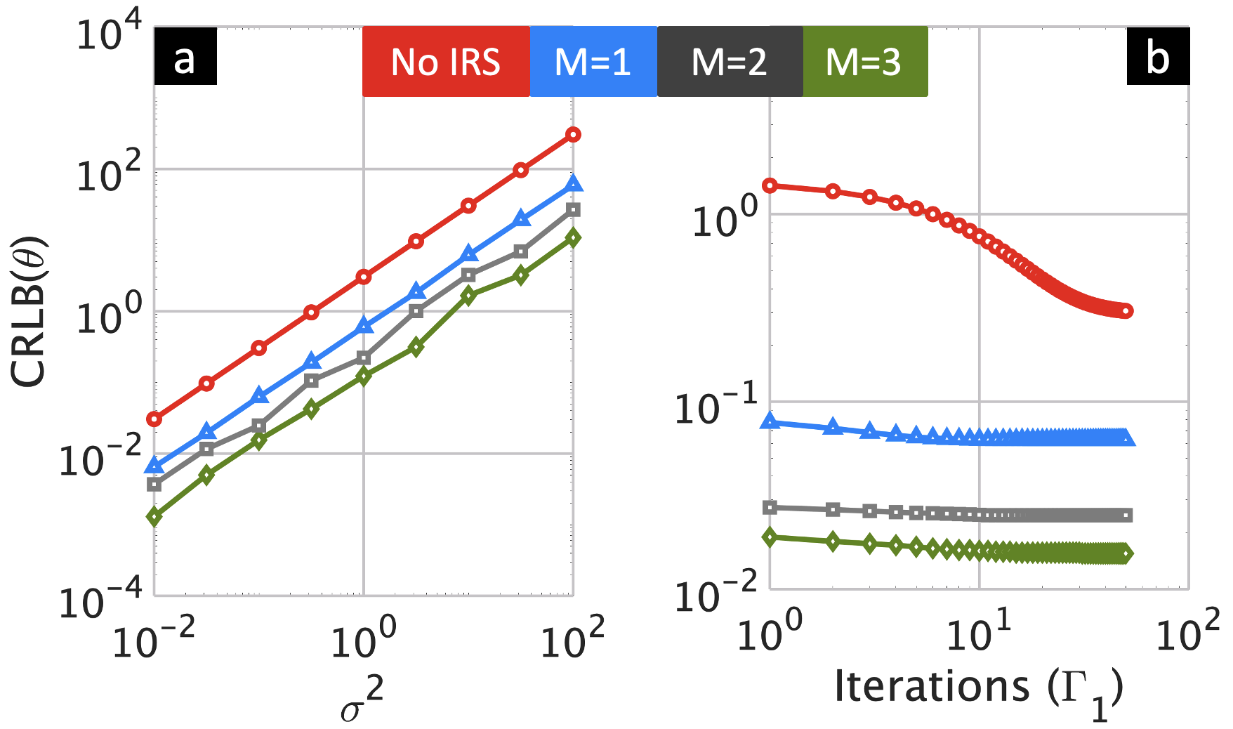
Fig. 1: The optimized CRLB of DoA versus (a) $\sigma^{2}$ for fixed number of iterations $\Gamma_{1}=50$, and (b) $\Gamma_{1}$ for fixed $\sigma^{2}=0.1$. In both experiments, $\Gamma_{2}$ was set to $20$.

We consider a radar, equipped with $N_{r}=N_{t}=8$ antennas for transmitter/receiver, positioned in the 2-D Cartesian plane at [$0$ m, $0$ m], sensing a target at [$5000$ m, $5000$ m]. We placed three IRS platforms with $N_{m}=8$ reflecting elements arranged as ULA with the first elements located at [$500$ m, $500$ m], [$500$ m, $-800$ m], and [$300$ m, $1300$ m]. The IRS platforms were deployed at far ranges w.r.t. the radar. Usually, distant targets tend to have obstructed or very weak LoS signal. In these cases, the received signal from the NLoS paths, i.e., the signal propagated through IRS platforms, is helpful in boosting the reflected LoS echo strength.

For a point-like target, given the radar, target and IRS positions, the corresponding radar–IRS_m and target–IRS_m angles $\theta_{ir,m}$ and $\theta_{ti,m}$, for $m\in\{1,\ldots,M\}$, are obtained through geometric computations. The complex reflectivity coefficients $\{\alpha_{m}\}$, which correspond to a Swerling 0 target model are generated from a $\mathcal{CN}(0,1)$. In Algorithm 1, we set $\Gamma_{1}=50$ and $\Gamma_{2}=20$ for all iterations. Throughout all our experiments the Lagrangian multiplier $\eta$ is tuned to $0.1$. Initially, all IRS platforms are set to impose zero phase shift $\upnu_{i}^{(0)}=\bm{0}_{{}_{MN_{m}}}$ for $i\in\{1,2\}$. The number of slow-time samples is set to $N=50$ and the samples in $\mathbf{X}^{(0)}$ are generated from a normal distribution. Fig. 1a illustrates that the multiple IRS-aided radar outperforms the single-IRS aided radar. Further, Fig. 1b indicates that iterations of Algorithm 1 result in a monotonically decreasing CRLB.

6 Summary

Waveform design for IRS-aided radar is relatively unexplored in prior works. In this context, this paper studies a new set of waveform design problems. Numerical experiments demonstrate that the deployment of multiple IRS platforms leads to a better achievable estimation performance compared to non-IRS and single-IRS systems. Some IRS model enhancements that should be accounted for in the future include the inter-IRS interference and quantization of the IRS phases.

References

• [1] Q. Wu and R. Zhang, “Towards smart and reconfigurable environment: Intelligent reflecting surface aided wireless network,” IEEE Communications Magazine, vol. 58, no. 1, pp. 106–112, 2019.
• [2] Ö. Özdogan, E. Björnson, and E. G. Larsson, “Intelligent reflecting surfaces: Physics, propagation, and pathloss modeling,” IEEE Wireless Communications Letters, vol. 9, no. 5, pp. 581–585, 2019.
• [3] S. Gong, X. Lu, D. T. Hoang, D. Niyato, L. Shu, D. I. Kim, and Y.-C. Liang, “Toward smart wireless communications via intelligent reflecting surfaces: A contemporary survey,” IEEE Communications Surveys & Tutorials, vol. 22, no. 4, pp. 2283–2314, 2020.
• [4] J. A. Hodge, K. V. Mishra, and A. I. Zaghloul, “Intelligent time-varying metasurface transceiver for index modulation in 6G wireless networks,” IEEE Antennas and Wireless Propagation Letters, vol. 19, no. 11, pp. 1891–1895, 2020.
• [5] J. A. Hodge, K. V. Mishra, B. M. Sadler, and A. I. Zaghloul, “Index-modulated metasurface transceiver design using reconfigurable intelligent surfaces for 6G wireless networks,” IEEE Journal of Selected Topics in Signal Processing, 2022, in press.
• [6] N. Torkzaban and M. A. A. Khojastepour, “Shaping mmwave wireless channel via multi-beam design using reconfigurable intelligent surfaces,” in IEEE Global Communications Conference Workshops, 2021, pp. 1–6.
• [7] M. F. Ahmed, K. P. Rajput, N. K. Venkategowda, K. V. Mishra, and A. K. Jagannatham, “Joint transmit and reflective beamformer design for secure estimation in IRS-aided WSNs,” IEEE Signal Processing Letters, vol. 29, pp. 692–696, 2022.
• [8] K. V. Mishra, A. Chattopadhyay, S. S. Acharjee, and A. P. Petropulu, “OptM3Sec: Optimizing multicast IRS-aided multiantenna DFRC secrecy channel with multiple eavesdroppers,” in IEEE International Conference on Acoustics, Speech and Signal Processing, 2022, pp. 9037–9041.
• [9] T. Wei, L. Wu, K. V. Mishra, and M. B. Shankar, “IRS-aided wideband dual-function radar-communications with quantized phase-shifts,” in IEEE Sensor Array and Multichannel Signal Processing Workshop, 2022, pp. 465–469.
• [10] A. M. Elbir, K. V. Mishra, M. B. Shankar, and S. Chatzinotas, “The rise of intelligent reflecting surfaces in integrated sensing and communications paradigms,” IEEE Network, 2022, in press.
• [11] S. Buzzi, E. Grossi, M. Lops, and L. Venturino, “Foundations of MIMO radar detection aided by reconfigurable intelligent surfaces,” IEEE Transactions on Signal Processing, vol. 70, pp. 1749–1763, 2022.
• [12] Z. Esmaeilbeig, K. V. Mishra, and M. Soltanalian, “IRS-aided radar: Enhanced target parameter estimation via intelligent reflecting surfaces,” in IEEE Sensor Array and Multichannel Signal Processing Workshop, 2022, pp. 286–290.
• [13] X. Song, J. Xu, F. Liu, T. X. Han, and Y. C. Eldar, “Intelligent reflecting surface enabled sensing: Cramér-Rao lower bound optimization,” arXiv preprint arXiv:2204.11071, 2022.
• [14] S. K. Dehkordi and G. Caire, “Reconfigurable propagation environment for enhancing vulnerable road users visibility to automotive radar,” in 2021 IEEE Intelligent Vehicles Symposium (IV), 2021, pp. 1523–1528.
• [15] Z. Esmaeilbeig, K. V. Mishra, A. Eamaz, and M. Soltanalian, “Cramér–Rao lower bound optimization for hidden moving target sensing via multi-irs-aided radar,” IEEE Signal Processing Letters, vol. 29, pp. 2422–2426, 2022.
• [16] Z. Wang, X. Mu, and Y. Liu, “STARS enabled integrated sensing and communications,” arXiv preprint arXiv:2207.10748, 2022.
• [17] T. Wei, L. Wu, K. V. Mishra, and M. Shankar, “Multi-IRS-aided doppler-tolerant wideband DFRC system,” arXiv preprint arXiv:2207.02157, 2022.
• [18] M. Alaee-Kerahroodi, M. Soltanalian, P. Babu, and M. R. B. Shankar, Signal Design for Modern Radar Systems.   Artech House, 2022.
• [19] Y. Li and S. Vorobyov, “Fast algorithms for designing unimodular waveform(s) with good correlation properties,” IEEE Transactions on Signal Processing, vol. 66, no. 5, pp. 1197–1212, 2017.
• [20] A. Bose, S. Khobahi, and M. Soltanalian, “Efficient waveform covariance matrix design and antenna selection for MIMO radar,” Signal Processing, vol. 183, p. 107985, 2021.
• [21] H. Hu, M. Soltanalian, P. Stoica, and X. Zhu, “Locating the few: Sparsity-aware waveform design for active radar,” IEEE Transactions on Signal Processing, vol. 65, no. 3, pp. 651–662, 2016.
• [22] M. Soltanalian, B. Tang, J. Li, and P. Stoica, “Joint design of the receive filter and transmit sequence for active sensing,” IEEE Signal Processing Letters, vol. 20, no. 5, pp. 423–426, 2013.
• [23] Z. Xu, C. Fan, and X. Huang, “MIMO radar waveform design for multipath exploitation,” IEEE Transactions on Signal Processing, vol. 69, pp. 5359–5371, 2021.
• [24] M. Naghsh, M. Soltanalian, P. Stoica, M. Modarres-Hashemi, A. De Maio, and A. Aubry, “A doppler robust design of transmit sequence and receive filter in the presence of signal-dependent interference,” IEEE Transactions on Signal Processing, vol. 62, no. 4, pp. 772–785, 2013.
• [25] A. Eamaz, F. Yeganegi, and M. Soltanalian, “One-bit phase retrieval: More samples means less complexity?” IEEE Transactions on Signal Processing, vol. 70, pp. 4618–4632, 2022.
• [26] M. Soltanalian and P. Stoica, “Designing unimodular codes via quadratic optimization,” IEEE Transactions on Signal Processing, vol. 62, no. 5, pp. 1221–1234, 2014.
• [27] J. Song, P. Babu, and D. Palomar, “Sequence design to minimize the weighted integrated and peak sidelobe levels,” IEEE Transactions on Signal Processing, vol. 64, no. 8, pp. 2051–2064, 2015.
• [28] E. Björnson, H. Wymeersch, B. Matthiesen, P. Popovski, L. Sanguinetti, and E. de Carvalho, “Reconfigurable intelligent surfaces: A signal processing perspective with wireless applications,” IEEE Signal Processing Magazine, vol. 39, no. 2, pp. 135–158, 2022.
• [29] K. V. Mishra and Y. C. Eldar, “Sub-Nyquist channel estimation over IEEE 802.11 ad link,” in IEEE International Conference on Sampling Theory and Applications, 2017, pp. 355–359.
• [30] S. M. Kay, Fundamentals of statistical signal processing: estimation theory.   Prentice-Hall, Inc., 1993.
• [31] J. Bezdek and R. Hathaway, “Convergence of alternating optimization,” Neural, Parallel & Scientific Computations, vol. 11, no. 4, pp. 351–368, 2003.
• [32] B. Tang, J. Tuck, and P. Stoica, “Polyphase waveform design for MIMO radar space time adaptive processing,” IEEE Transactions on Signal Processing, vol. 68, pp. 2143–2154, 2020.