^∗Corresponding author. Email: sryee@physnet.uni-hamburg.de (S.R.); tim.wehling@physik.uni-hamburg.de (T.O.W.)

Abstract

Mott-Hubbard and Hund electron correlations have been realized thus far in separate classes of materials. Here, we show that a single moiré homobilayer encompasses both kinds of physics in a controllable manner. We develop a microscopic multiband model that we solve by dynamical mean-field theory to nonperturbatively address the local many-body correlations. We demonstrate how tuning with twist angle, dielectric screening, and hole density allows us to switch between Mott-Hubbard and Hund correlated states in a twisted WSe₂ bilayer. The underlying mechanism is based on controlling Coulomb-interaction-driven orbital polarization and the energetics of concomitant local singlet and triplet spin configurations. From a comparison to recent experimental transport data, we find signatures of a filling-controlled transition from a triplet charge-transfer insulator to a Hund-Mott metal. Our finding establishes twisted transition metal dichalcogenides as a tunable platform for exotic phases of quantum matter emerging from large local spin moments.

Keywords: moiré materials, strongly correlated electrons, Hund physics, Mott-Hubbard physics, charge-transfer insulator, dynamical mean-field theory

Strong electron correlations in quantum materials are often associated with two different categories. In single-orbital Mott-Hubbard systems PALee ; Arovas , strong correlations promoted by large onsite Coulomb repulsion Imada ; Phillips lead from Mott insulating to metallic and unconventional superconducting phases upon doping. In contrast, distinct Hund correlations emerge in materials with almost degenerate multiple orbitals at low energies Georges . Prominent examples are iron-based superconductors and ruthenates Haule ; Mravlje ; Yin1 ; Medici_2014 ; Medici_2017 ; Fanfarillo_2 ; Miao ; HJLee ; Fernandes . Here, Hund coupling $J$ induces the formation of large local spin moments and impedes the quasiparticle coherence down to very low temperatures Nevidomskyy ; Yin_power ; Aron ; Stadler1 ; Horvat ; Drouin-Touchette . Hund physics can also give rise to many intriguing broken-symmetry phases, such as spin-triplet superconductivity Hoshino ; Vafek ; Coleman , charge orders Isidori ; Ryee ; Ryee3 , and exciton condensates Kunes ; Geffroy ; Werner_exciton .

From a theoretical perspective, Mott-Hubbard and Hund physics arise, respectively, in the strong and weak crystal-field limits of multiorbital Hamiltonians Georges ; Ryee4 . Material-wise, however, Mott-Hubbard and Hund correlated systems have appeared thus far as separate classes of compounds. This missing bridge is related to chemical constraints on the tunability of “conventional” materials. In this respect, moiré heterostructures constitute a complementary domain of correlated electron physics Kennes .

In this work, twisted transition metal dichalcogenide (TMD) homobilayers are shown to host both Mott-Hubbard and Hund physics. We demonstrate how Coulomb interactions facilitate the promotion of electrons to higher energy moiré bands. As a consequence, multiorbital correlations can arise even in situations in which moiré band theory suggests single-orbital physics. We combine a microscopic multiband continuum model with dynamical mean-field theory (DMFT) Georges_DMFT to demonstrate how twist angle ($\theta$), dielectric constant ($\epsilon$), and hole density ($n$) (see Figure 1a) enable continuous switching between Mott-Hubbard and Hund physics (Figure 1b) for the experimentally most relevant case of twisted WSe₂ (tWSe₂) Scuri ; LWang ; 2020_flatband ; Andersen ; Ghiotto ; bilayer2022 . A comparison to recent transport experiments LWang reveals a filling-controlled transition from a novel “triplet charge-transfer insulator” to a strongly correlated Hund-Mott metal. The multiorbital spin correlations are expected to control, both, excitonic physics and the emergence of magnetism and superconductivity in the system.

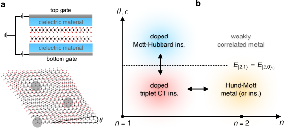
Figure 1: (a) Twisted TMD homobilayer surrounded by a dielectric material in the side view (top) and top view (bottom). Voltages applied to the top and bottom gates control the hole density $n$. The emergent moiré superlattice is illustrated by gray circles marking the AA stacked regions. (b) Nature of electron correlations depending on hole density $n$, twist angle $\theta$, and dielectric constant $\epsilon$ that effectively encodes screening processes affecting the magnitude of Coulomb interactions.

We begin with the AA-stacked bilayer WSe₂, where every W and Se atom in the top layer are located on top of the same type of atom in the bottom layer. Twisting by a small angle $\theta$ (Figure 1a), a long-wavelength moiré pattern with concomitant moiré Brillouin zone (mBZ) (see Figure 2a) emerges. Due to the strong spin-valley locking, the topmost valence bands of each monolayer (schematically shown in Figure 2b) exhibit solely spin-$\uparrow$ character in the $K$ valley and spin-$\downarrow$ in the $K^{\prime}$ valley Wu_1 . The top- and bottom-layer valence bands hybridize in each valley through interlayer tunneling, which leads, by twisting the two layers, to minibands at low energies.

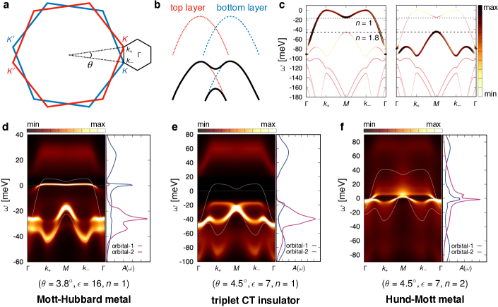
Figure 2: (a) Brillouin zones of the top (red) and bottom (blue) layers along with the resulting mBZ (black). (b) Upper: schematic band dispersion of the top (red) and bottom (blue) layer valence states whose valence band maxima are located, respectively, at $k_{+}$ and $k_{-}$ points. Lower: schematic moiré bands resulting from the hybridization between the top and bottom layer bands. (c) The band characters are represented by color intensity for orbital-1 (left panel; $\eta=1$) and orbital-2 (right panel; $\eta=2$). The spin-$\uparrow$ band originating from the $K$ valley and the spin-$\downarrow$ band from $K^{\prime}$ are degenerate. The horizontal dashed lines indicate Fermi levels for two different hole fillings within a rigid-band model. (d, e, f) Influence of many-body effects on excitation spectra as obtained from DMFT. The momentum-dependent spectral functions $A(\mathbf{k},\omega)$ (color coded) and the local density of states $A(\omega)$ are shown for representative examples of correlated regimes realized in tWSe₂: (d) Mott-Hubbard metal, (e) triplet CT insulator, and (f) Hund-Mott metal. The chemical potential is at $\omega=0$. White solid lines indicate the noninteracting continuum bands for the same $n$.

A useful strategy to describe the noninteracting band structure associated with the long-wavelength moiré potential is the continuum model Santos ; Bistritzer ; Pan_1 ; Wu_1 ; Devakul ; see Supporting Information. Our moiré bands in Figure 2c are consistent with large-scale ab initio calculations at a nearby angle of $\theta=5.08^{\circ}$ Devakul ; LWang . We below focus on $\theta$ in a range of $3.5^{\circ}\leq\theta\leq 6.5^{\circ}$, in light of recent experiments LWang ; Ghiotto . At first glance, only the topmost band seems to play a role for hole filling up to $n\simeq 1.8$; see dashed lines in Figure 2c. One of our main conclusions, however, is that many-body interactions can significantly modify this picture, which leads to multiorbital (or multiband) physics already at $n=1$, contrary to the current belief.

To investigate the impact of electron correlations, we derive a lattice model for the two topmost moiré bands. These bands resemble the parabolic top (bottom) layer states near $k_{+}$ ($k_{-}$) and display an avoided crossing in between them (schematically shown in Figure 2b). Using bonding-antibonding combinations of top and bottom layer states we construct Wannier functions (Supporting Information), $|\widetilde{c}_{i\eta\sigma}\rangle$, from the topmost two bands. Here, $i$ denotes the site, $\eta\in\{1,2\}$ the orbital, and $\sigma\in\{\uparrow,\downarrow\}$ the spin. The decomposition of the two topmost bands into the Wannier orbitals in Figure 2c shows that the topmost (second) displays predominantly $|\widetilde{c}_{i1\sigma}\rangle$ ($|\widetilde{c}_{i2\sigma}\rangle$) character.

We now arrive at the two-orbital Hamiltonian $\mathcal{H}=H_{\mathrm{k}}+\sum_{i}H^{i}_{\mathrm{loc}}$. We hereafter switch to the hole representation by performing a particle-hole transformation: $\widetilde{c}_{i\eta\sigma}\rightarrow d^{\dagger}_{i\eta\sigma}$. $H_{\mathrm{k}}$ is the kinetic term consisting of inter-cell hopping amplitudes (see Supporting Information). $H^{i}_{\mathrm{loc}}$ contains all the nonnegligible local terms acting at a site $i$:

$$\begin{split}H^{i}_{\mathrm{loc}}&=\sum_{\eta}U_{\eta}{n_{i\eta\uparrow}n_{i\eta\downarrow}}+\sum_{\eta<\eta^{\prime},\sigma\sigma^{\prime}}(U^{\prime}-J\delta_{\sigma\sigma^{\prime}}){n_{i\eta\sigma}n_{i\eta^{\prime}\sigma^{\prime}}}\\ &+\sum_{\eta\neq\eta^{\prime}}J(d^{\dagger}_{i\eta\uparrow}d^{\dagger}_{i\eta^{\prime}\downarrow}d_{i\eta\downarrow}d_{i\eta^{\prime}\uparrow}+d^{\dagger}_{i\eta\uparrow}d^{\dagger}_{i\eta\downarrow}d_{i\eta^{\prime}\downarrow}d_{i\eta^{\prime}\uparrow})+\sum_{\eta,\sigma}\Big{(}\frac{\Delta}{2}(-1)^{\eta}-\mu\Big{)}n_{i\eta\sigma}.\end{split}$$ (1)

$n_{i\eta\sigma}=d^{\dagger}_{i\eta\sigma}d_{i\eta\sigma}$ is the hole number operator. $\mu$ is the chemical potential that determines the hole filling and is experimentally controllable via gate voltage (see Figure 1a). $U_{\eta}$ and $U^{\prime}$ are intra- and inter-orbital Coulomb repulsions, respectively. $J$ is the Hund exchange coupling. The real-space shape of the Wannier functions leads to an unusual hierarchy of Coulomb terms: $U_{1}>U^{\prime}>U_{2}>J$. The values of $U_{\eta}$, $U^{\prime}$, and $J$ are tunable via twist angle and dielectric screening, where the latter approximately modifies the Coulomb potential $v_{c}(\mathbf{r},\mathbf{r}^{\prime})=e^{2}/(\epsilon|\mathbf{r}-\mathbf{r}^{\prime}|)$ (see Supporting Information for further analysis). $\Delta$ ($\Delta>0$) is the local energy-level splitting between the two orbitals and plays the role of a crystal field. To address nonperturbatively the effects of the local many-body interactions, we solve the model using DMFT DMFT (see Supporting Information). For hole fillings smaller than $n=1$ ($n=\sum_{i\eta\sigma}\langle n_{i\eta\sigma}\rangle/N_{\mathrm{s}}$ where $N_{\mathrm{s}}$ is the number of lattice sites), the low-energy physics is essentially captured by a single-orbital model. We thus focus on a range of $1\leq n\leq 2$.

We first discuss how interactions affect the electron/hole excitation spectra. Central observables are the momentum-dependent spectral function $A(\mathbf{k},\omega)$ and the local density of states $A(\omega)$, which can be measured by photoemission or scanning tunneling spectroscopies, respectively. Figures 2d–f presents $A(\mathbf{k},\omega)$ and $A(\omega)$ of three different correlated states. Many-body interactions significantly modify the excitation spectra compared to the noninteracting cases. Specifically, incoherent upper Hubbard bands (located far above $\omega=0$) stemming from orbital-1 are clearly visible in all of the three cases. Lower Hubbard bands (located below $\omega=0$) also form, but they are smeared over wider energy ranges due to the hybridization with the relatively coherent states of orbital-2 ($\eta=2$) character.

Looking into the spectra in more detail reveals distinct features in each regime. In the Mott-Hubbard case (Figure 2d), low-energy charge excitations involve almost exclusively orbital-1. We also find that a flatter dispersion (i.e., enhanced quasiparticle mass) emerges near $\omega=0$ compared to the noninteracting one due to a large band-renormalization promoted by Mott-Hubbard physics. Hubbard models based solely on orbital-1 can describe this case, as was done and reported previously Zang_1 ; Zang_2 ; Wietek ; Klebl ; Wu ; Belanger .

For a smaller $\epsilon$ (i.e., weaker dielectric screening), however, the single-orbital description breaks down. In Figure 2e, a pronounced charge gap emerges at one-hole filling, which demonstrates a phase transition to a correlated insulator by many-body interactions. The nature of this insulating phase is clearly distinct from what is expected from single-orbital Mott-Hubbard physics. Namely, the lowest-energy charge excitations involve both orbital characters on the hole side. As a consequence, doped holes will occupy both orbitals. Upon further hole doping (energies below $\omega\simeq-20$ meV), almost all the holes should go into orbital-2; see the orbital-2 weight pronounced in $A(\omega)$ near $\omega\simeq-40$ meV. This type of insulator is reminiscent of charge-transfer (CT) insulators ZSA . Importantly, however, due to the $J$ in the system, two holes distributed over both orbitals in a site should favor a local triplet, as opposed to the singlet realized in many typical CT insulators like cuprates ZR . We, thus, call this phase a “triplet CT insulator”.

Heavy hole doping the triplet CT insulator up to $n=2$ (Figure 2f) gives rise to a metal with strong mass enhancement and with broad incoherent excitations up to about $\pm 80$ meV. Here, both orbitals contribute again to the low-energy spectral weight. Since both orbitals are almost equally occupied in this regime, $J$ plays a crucial role in promoting strong correlations, which will be analyzed further below.

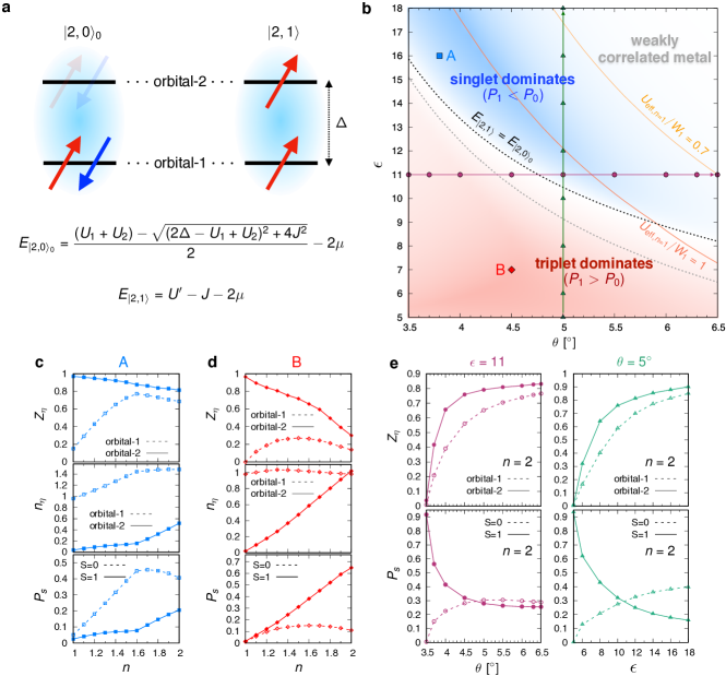
Figure 3: (a) Illustration of the orbital-polarized two-hole singlet state $|2,0\rangle_{0}$ (left) and the two hole triplet states $|2,1\rangle$ (right), and their energies. Here, only one of the three $|2,1\rangle$ states is plotted. The arrows denote spin-up (red) or spin-down (blue) holes. (b) Nature of electronic states relevant for the hole filling range of $1\leq n\leq 2$ as function of twist angle ($\theta$) and dielectric constant ($\epsilon$). Two regimes are highlighted by colors: blue for singlet-dominant correlations (i.e., $P_{1}<P_{0}$) and red for triplet-dominant correlations (i.e., $P_{1}>P_{0}$), where $P_{S}$ denotes the probability of a given spin $S$ to be realized in the two-hole subspace of $H^{i}_{\mathrm{loc}}$. The black (gray) dotted line represents the “phase boundary” below which $E_{|2,1\rangle}<E_{|2,0\rangle_{0}}$ ($U_{1}-U^{\prime}>\Delta$). The four different symbols indicate the twisted angles and dielectric constants used in the DMFT scans of the phase diagram. To estimate the strength of electron correlations, we look at the ratio of the bandwidth to the “effective” local Coulomb interactions $U_{\mathrm{eff},n}$ defined by $U_{\mathrm{eff},n}\equiv\mathcal{E}_{n+1}+\mathcal{E}_{n-1}-2\mathcal{E}_{n}$ Georges . Here, $\mathcal{E}_{n}$ denotes the lowest eigenvalue of $H^{i}_{\mathrm{loc}}$ in the $n$-hole subspace. Near $n\simeq 1$, one would expect strong correlations below the line defined by $U_{\mathrm{eff},n=1}=W_{1}$ (orange line). $W_{1}$ is the bandwidth of the lowest-lying band. (c, d) DMFT results for orbital-dependent quasiparticle weight $Z_{\eta}$, orbital-resolved hole filling $n_{\eta}$, and $P_{S}$ as a function of hole density $n$ for (c) $\theta=3.8^{\circ}$ and $\epsilon=16$ (i.e., $P_{1}<P_{0}$) and (d) $\theta=4.5^{\circ}$ and $\epsilon=7$ (i.e., $P_{1}>P_{0}$). (e) DMFT results for $Z_{\eta}$ and $P_{S}$ at fixed hole filling $n=2$ as a function of $\theta$ at $\epsilon=11$ (left panels) and $\epsilon$ at $\theta=5^{\circ}$ (right panels).

To pinpoint the microscopic origin of the distinct correlations revealed by the spectral functions, we look at the eigenstates and eigenvalues of $H^{i}_{\mathrm{loc}}$ in the two-hole subspace. Here, two types of lowest-energy states are competing in energy: an orbital-polarized singlet $|N=2,S=0\rangle_{0}$ ($N$: the number of holes, $S$: total spin of $N$ holes) and triply degenerate states $|2,1\rangle$, where each orbital is occupied by one hole and total spin $S=1$. See Figure 3a for a schematic illustration of these states and corresponding energies. Note that while $|2,0\rangle_{0}$ is a mixed state to be exact, i.e., $|2,0\rangle_{0}=\alpha d^{\dagger}_{i1\downarrow}d^{\dagger}_{i1\uparrow}|0\rangle+\beta d^{\dagger}_{i2\downarrow}d^{\dagger}_{i2\uparrow}|0\rangle$, the contribution from the second term is found to be negligible (i.e., $|\alpha|^{2}\gg|\beta|^{2}$) in a regime where $|2,0\rangle_{0}$ is the lowest-energy multiplet. Refer to Supporting Information for all of the eigenvalues and eigenstates of $H^{i}_{\mathrm{loc}}$. Indeed, we find that the energy of $|2,0\rangle_{0}$ ($E_{|2,0\rangle_{0}}$) is lower than that of $|2,1\rangle$ ($E_{|2,1\rangle}$) in the Mott-Hubbard regime (Figure 2d), whereas it is the opposite in the triplet CT insulator (Figure 2e) and in the Hund-Mott metal regimes (Figure 2f). Thus, the nature of the correlations can be traced back to the local two-hole multiplets even at $n=1$.

One natural question arises: What drives the occupation of orbital-2? We find to zeroth-order in $J$, which is the smallest energy scale in $H^{i}_{\mathrm{loc}}$, $E_{|2,1\rangle}\approx U^{\prime}-2\mu$ and $E_{|2,0\rangle_{0}}\approx U_{1}-\Delta-2\mu$. Thus, $E_{|2,1\rangle}<E_{|2,0\rangle_{0}}$ means that $U_{1}-U^{\prime}>\Delta$, i.e. occupation of orbital-2 is favorable if the difference between intra- and inter-orbital Coulomb repulsion exceeds the crystal field splitting $\Delta$. Since $\Delta$ is unchanged by $\epsilon$ and $U_{1}>U^{\prime}$, orbital-2 can be occupied when the dielectric screening is sufficiently weak (see also Supporting Information).

We now conceive a twist-angle and dielectric-constant dependent “phase” diagram, see Figure 3b, where we denote the nature of electron correlations. Here, one can identify a boundary, black dotted line defined by $E_{|2,1\rangle}=E_{|2,0\rangle_{0}}$, below (above) which triplet (singlet) dominates in the two-hole eigenstates of $H^{i}_{\mathrm{loc}}$. This boundary is indeed also well approximated by the requirement of $U_{1}-U^{\prime}=\Delta$ (gray dotted line).

Insight into the correlation strength is obtained by the orbital-dependent quasiparticle weight $Z_{\eta}$. This quantity corresponds to the inverse of the quasiparticle mass enhancement within DMFT via $Z_{\eta}=(m^{*}/m_{b})_{\eta}^{-1}$ where $m^{*}$ ($m_{b}$) is the renormalized (bare) band mass. Thus, strong correlations feature small or vanishing $Z_{\eta}$. We investigate the results in case A in Figure 3b for the Mott-Hubbard and case B for the triplet CT regimes. We find that $Z_{1}\simeq 0.15$ in A and $Z_{1}=0$ in B (upper panels of Figures 3c and d). On the other hand, $Z_{2}\simeq 1$ for both cases, since orbital-2 is almost empty when $n=1$. These small $Z_{1}$ values for both cases corroborate the strong correlations of orbital-1 character captured in the excitation spectra of A and B at $n=1$, as presented in Figures 2d and e.

In contrast, near $n\simeq 2$, strong correlations are found only when triplet states are predominant (the region where $E_{|2,1\rangle}<E_{|2,0\rangle_{0}}$ in Figure 3b). Namely, while both orbitals are weakly correlated, i.e., $Z_{\eta}\gtrapprox 0.7$ in A, they are almost equally occupied ($n_{1}\simeq n_{2}\simeq 1$) due to the CT nature and are both strongly correlated in B (Figures 3c and d). Investigating the quasiparticle scattering rate $\Gamma_{\eta}$ also reveals strong correlations in B at $n=2$ in that $\Gamma_{1}\simeq 0.7T$ and $\Gamma_{2}\simeq 0.5T$ ($T=0.005W_{1}\simeq 3.56$ K), which are comparable to the thermal fluctuation rate, which means scattering close to the Planckian limit.

We find that the strong correlation near $n=2$ accompanies the predominance of triplets ($S=1$) over singlets ($S=0$) in the local two-hole states. Based on the Kondo picture of Hund physics, a large local spin moment impedes the formation of quasiparticles by protracting the Kondo screening Nevidomskyy ; Yin_power ; Aron ; Stadler1 ; Horvat ; Drouin-Touchette . In this respect, we present $P_{S}$ (the probability of a given spin $S$ to be realized in the two-hole subspace of $H^{i}_{\mathrm{loc}}$) in the bottom panels of Figures 3c and d. It shows that $P_{1}<P_{0}$ in A whereas $P_{1}>P_{0}$ in B near $n=2$, which is also consistent with the energetics of $|2,1\rangle$ and $|2,0\rangle_{0}$. The dichotomy between these two points is not specific to the parameter choice, but a general feature related to which spin state is dominant in the local two-hole states. Indeed, the same correlation between $Z_{\eta}$ and $P_{S}$ is found by varying either twist angle or dielectric constant (Figure 3e). The role of $J$ at $n=2$ is particularly pronounced because it not only impedes the spin-Kondo screening, but also enhances the atomic (Mott) gap Georges . In this respect, we call this regime a “Hund-Mott” metal [or, insulator when $Z_{\eta}=0$ at $n=2$; see the results for ($\theta=3.5^{\circ}$, $\epsilon=11$) or ($\theta=5^{\circ}$, $\epsilon=5$) in Figure 3e] following the term used in Ref. Springer .

Having established all of the regimes of Figure 1b, we now discuss implications of our findings for the understanding of recent experiments. Figure 4a presents the resistance $R$ of tWSe₂ measured at $\theta=4.2^{\circ}$ in Ref. LWang under hBN encapsulation. Given the dielectric tensor of bulk hBN ($\epsilon_{\parallel}=6.9$ for in-plane and $\epsilon_{\perp}=3.8$ for out-of-plane values) Laturia2018 , we assume that $\epsilon<10$, which will put this sample into the regime of Hund physics (c.f. Figure 3). The experimentally measured resistance features peaks around the (experimentally estimated) integer fillings $n=1$ and $n=2$. Extrinsic disorder or impurity scattering as well as phonons will contribute to the magnitude of the resistance. We show, however, in the following, that the “two-peak” structure near integer fillings can be naturally explained by an electronic origin. To this end, we consider the transport scattering rate $(\Gamma/Z)_{\eta}$ which is responsible for degrading conductivity owing to electron correlations.

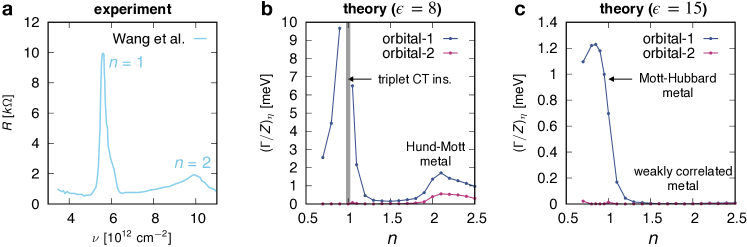
Figure 4: Comparison between (a) the experimental resistance $R$ as a function of hole density $\nu$ at $T=1.8$ K and $\theta=4.2^{\circ}$, reported in Ref. LWang and (b, c) theoretically calculated transport scattering rates $(\Gamma/Z)_{\eta}$ at $T\simeq 2.97$ K and $\theta=4.2^{\circ}$. (b) Hund physics dominant regime; $\epsilon=8$. $(\Gamma/Z)_{1}\rightarrow\infty$ at $n=1$. (c) Mott-Hubbard physics dominant regime; $\epsilon=15$.

Using the same twist angle as in the experiment ($\theta=4.2^{\circ}$) and approximating the dielectric constant of $\epsilon=8$, we find the transport scattering rate shown in Figure 4b. Two peaks emerge around integer fillings $n=1$ and $n=2$ in the doping-dependence of $(\Gamma/Z)_{1}$, as also seen in the experiment. In contrast, calculations in the Mott-Hubbard case do not feature the two-peak structure (Figure 4c; see also Supporting Information). The reason is the weakening of correlations upon doping toward $n=2$ in the Mott-Hubbard case, which stands in contrast to the doped triplet CT regime and Hund-Mott metal. Thus, the two-peak structure in the experimentally measured resistance signals prevailing strong electron correlations by Hund physics.

Other experiments can potentially be used to detect direct signatures of Hund physics in this system. Since an instantaneous local triplet is promoted by Hund physics, fast local probes like x-ray absorption or emission spectroscopies are relevant techniques. In TMDs, spin-valley coupling sets special optical selection rules and it might be possible to probe local moments using optical techniques. We speculate that triplet formation will affect spin and valley lifetimes of the excitonic species.

Our study shows that tWSe₂ implements the first system where a tuning between Mott-Hubbard and Hund physics is continuously possible. Near $\theta\simeq 5^{\circ}$ we expect a change between Hund and Mott-Hubbard physics under typical experimental hBN encapsulation conditions (Figure 3b), which is likely a crossover if it involves metallic states. Genuine phase transitions may also be possible if symmetry breaking is involved. The system at hand might facilitate experimental approaches to this question.

What consequences can be expected from Hund physics emerging in the hole fillings of $n>1$? First, Hund-driven pairing mechanisms Hoshino ; Vafek ; Coleman may give rise to superconductivity. In particular, enhanced local spin fluctuations driven by the competition between a singlet and triplet near $\theta\simeq 5^{\circ}$ and $\epsilon\simeq 10$ may induce $s$-wave spin-triplet pairing Hoshino . Near $n=2$, the spin-state transition (or crossover) can trigger excitonic instabilities both in and out-of equilibrium Kunes ; Geffroy ; Werner_exciton , accompanying the transition between the Hund-Mott state and a weakly correlated metal (Figure 1b).

Thus, tWSe2 and related TMD homobilayers Yu_2021 open the gate for the realization and control of novel broken-symmetry phases in the regime of triplet correlations and in the hitherto unexplored spin-crossover region. Similar physics may also be expected in TMD heterobilayers where higher-lying orbitals appear within reach by charge doping YZhang .

Supporting Information

The continuum model (S1), Wannier functions in the bonding-antibonding-orbital basis (S2), Hopping amplitudes and local interaction tensor elements (S3), Coulomb versus Keldysh potential (S4), Method (S5), Eigenvalues and eigenstates in the atomic limit and the atomic gap (S6), The effect of interorbital hopping on the doped Mott-Hubbard regime (S7), The effect of intersite density-density interactions (S8), and Mott-Hubbard versus Hund physics on the transport scattering rate (S9).

Acknowledgements

The authors are grateful to M. J. Han and L. Klebl for useful discussions. This work is supported by the Cluster of Excellence ‘CUI: Advanced Imaging of Matter’ of the Deutsche Forschungsgemeinschaft (DFG) - EXC 2056 - project ID 390715994, by DFG priority program SPP 2244 (WE 5342/5-1 project No. 422707584) and the DFG research unit FOR 5242 (WE 5342/7-1, project No. 449119662).

Supporting Information for
Switching between Mott-Hubbard and Hund physics in moiré quantum simulators

Siheon Ryee¹ and Tim O. Wehling^1,2
1I. Institute of Theoretical Physics, University of Hamburg, Notkestrasse 9, 22607 Hamburg, Germany
²The Hamburg Centre for Ultrafast Imaging, Luruper Chaussee 149, 22761 Hamburg, Germany

S1 The continuum model

The continuum model Hamiltonian for spin-$\uparrow$ moiré bands of $K$-valley twisted transition-metal dichalcogenides reads Wu_2 ; Pan_1 ; Devakul

$$H_{\uparrow}=\begin{pmatrix}\frac{-\hbar^{2}(\mathbf{k}-k_{+})^{2}}{2m_{b}}+\Delta_{+}(\mathbf{r})&\Delta_{T}(\mathbf{r})\\ \Delta^{\dagger}_{T}(\mathbf{r})&\frac{-\hbar^{2}(\mathbf{k}-k_{-})^{2}}{2m_{b}}+\Delta_{-}(\mathbf{r})\end{pmatrix},$$ (S1)

where $k_{\pm}$ are the corners of the moiré Brillouin zone, resulting from $\pm\theta/2$ rotation of top ($+$) and bottom ($-$) layers [see Figure 2a in the main text]. The Hamiltonian for spin-$\downarrow$ bands (originating from top and bottom layer $K^{\prime}$-valley valence states) is obtained by time-reversal conjugation of Eq. (S1). The intralayer potential $\Delta_{\pm}(\mathbf{r})$ and interlayer tunneling $\Delta_{T}(\mathbf{r})$ are given by Wu_2 ; Pan_1 ; Devakul

$$\begin{split}\Delta_{\pm}(\mathbf{r})=2V\sum_{j=1,3,5}\mathrm{cos}(\mathbf{g}_{j}\cdot\mathbf{r}\pm\phi),\\ \Delta_{T}(\mathbf{r})=\omega(1+e^{-i\mathbf{g}_{2}\cdot\mathbf{r}}+e^{-i\mathbf{g}_{3}\cdot\mathbf{r}}).\end{split}$$ (S2)

Here, $\mathbf{g}_{j}$ are reciprocal lattice vectors of the moiré superlattice, which are obtained by $(j-1)\pi/3$ counterclockwise rotation of $\mathbf{g}_{1}=4\pi\theta/(a_{0}\sqrt{3})\hat{x}$ with $a_{0}$ being the lattice constant of monolayer WSe₂ ($a_{0}=3.317$ Å). The resulting band structure largely depends on four adjustable parameters: $m_{b}$, $V$, $\phi$, and $\omega$. We adopt $m_{b}=0.43m_{e}$ ($m_{e}$: free electron mass) and $(V,\phi,\omega)=(9\leavevmode\nobreak\ \mathrm{meV},128^{\circ},18\leavevmode\nobreak\ \mathrm{meV})$ which were estimated previously by density functional theory calculations Devakul .

S2 Wannier functions in the bonding-antibonding-orbital basis

To investigate the impact of electron correlations, we derive a lattice model and analyze the band structure in detail. The topmost band closely resembles the parabolic top and bottom layer valence states near $k_{+}$ and $k_{-}$, respectively. Interlayer coupling opens a hybridization gap around the crossing of the two topmost moiré bands (schematically shown in Figure 2b of the main text), where the eigenstates resemble bonding/antibonding combinations of the top and bottom layer valence band states. To construct a lattice model, we thus project two “layer-localized” Gaussian trial functions (one for each layer) centered at the triangular sites of the moiré superlattice onto the two topmost bands. Then, we construct corresponding Wannier functions following the recipe of Ref. Witt via the Löwdin orthogonalization Marzari . As a final step, we perform a basis transformation to a “bonding-antibonding-orbital” (BAO) basis as follows:

$$|\widetilde{c}_{i1\sigma}\rangle=\frac{|c_{it\sigma}\rangle+|c_{ib\sigma}\rangle}{\sqrt{2}},\leavevmode\nobreak\ |\widetilde{c}_{i2\sigma}\rangle=\frac{|c_{it\sigma}\rangle-|c_{ib\sigma}\rangle}{\sqrt{2}}.$$ (S3)

Here, $|c_{it(b)\sigma}\rangle$ denotes a layer-localized Wannier state residing mainly in the top (bottom) layer. $\sigma\in\{\uparrow,\downarrow\}$ is the spin and $i$ the site index. $|\widetilde{c}_{i1\sigma}\rangle$ and $|\widetilde{c}_{i2\sigma}\rangle$ are BAOs, respectively.

Figure S1: (a) The band characters are represented by color intensity for orbital-1 (top panel; $\eta=1$) and orbital-2 (bottom panel; $\eta=2$). The spin-$\uparrow$ band originating from the $K$ valley and the spin-$\downarrow$ bands from $K^{\prime}$ are degenerate. The horizontal dashed lines indicate Fermi levels for two different hole fillings $n$ within a rigid-band model. Here, $n\equiv\frac{1}{N_{\mathbf{k}}}\sum_{\mathbf{k}l\sigma}n_{\mathbf{k}l\sigma}$ with $n_{\mathbf{k}l\sigma}$ being the layer ($l$) and spin ($\sigma$) resolved hole density at a given $\mathbf{k}$. $N_{\mathbf{k}}$ is the number of $\mathbf{k}$ points. (b) Leftmost: the real space Wannier density $|w_{i\eta}(\mathbf{r})|^{2}$. $|w_{i\eta}(\mathbf{r})|^{2}$ is the sum of layer-resolved densities which are plotted in the middle panels. Rightmost: the probability density of continuum-band wave functions $\sum_{\mathbf{k}}|\psi_{\mathbf{k},m}(\mathbf{r})|^{2}$ for $m=1$ (upper panel) and $m=2$ (lower panel).

The relative weight of BAOs in the two topmost continuum bands is presented using color intensity in Figure S1(a). Indeed, this basis nicely captures the two topmost bands with interorbital hybridization along the $k_{\pm}$–$M$ lines. We hereafter omit the spin index for simplicity. Figure S1(b) presents the real space densities of the BAOs $|w_{i\eta}(\mathbf{r})|^{2}$ located at a triangular lattice site $i$. $\eta\in\{1,2\}$ denotes BAOs, and $\mathbf{r}$ is the real space position vector. Interestingly, $|w_{i1}(\mathbf{r})|^{2}$ is peaked at the center of the hexagon, whereas $|w_{i2}(\mathbf{r})|^{2}$ is largest along a ring encompassing AB and BA moiré sites. These contrasting real-space profiles of two orbitals are manifestations of the same characteristics of the corresponding continuum-band wave functions; see the right panels in Figure S1(b) for $\sum_{\mathbf{k}}|\psi_{\mathbf{k},m}(\mathbf{r})|^{2}$ ($\mathbf{k}$ is the crystal-momentum of moiré superlattice and $m$ the band index numbered from top to bottom bands). The same is true also for the entire range of $\theta$ ($3.5^{\circ}\leq\theta\leq 6.5^{\circ}$) which we consider in this work. Thus, we conclude that two BAOs well represent the continuum-model band structure of the two topmost bands in this range of $\theta$. Note in passing that for smaller twist angles outside this range (around $\theta\sim 1^{\circ}$), a honeycomb lattice with one orbital for each sublattice properly models the two topmost bands Devakul .

S3 Hopping amplitudes and local interaction tensor elements

Figure S2: (a) The $\theta$-dependence of the hopping amplitudes between the two orbitals. (b) The sign (red for spin-$\uparrow$ and blue for spin-$\downarrow$) of imaginary hopping $t^{(1)}_{12}$ from a given site (black circle) to its NNs (red circles) in the triangular lattice. (c) Comparison between the continuum-model and the two-orbital-model bands using hopping amplitudes presented in (a) at $\theta=5^{\circ}$. The bands are plotted in terms of hole representation. (d) The $\theta$-dependence of $U_{\eta}$, $U^{\prime}$, and $J$.

Figure S2(a) presents the magnitude of $l$-th nearest neighbor (NN) hopping amplitudes $t^{(l)}_{\eta\eta^{\prime}}$ of holes between $\eta$ and $\eta^{\prime}$ orbitals ($\eta,\eta^{\prime}=1,2$). All the hopping amplitudes are real numbers except for $t^{(1)}_{12}$ which is purely imaginary and acquires different signs depending on the spin and the direction of hopping [Figure S2(b)]. We find from Figure S2(a) that all the hopping amplitudes increase with $\theta$, which is consistent with the general observations in related twisted transition-metal dichalcogenides: the moiré periodicity decreases and concomitantly the moiré superlattice constant gets reduced resulting in the increase of hoppings LWang ; Pan_1 ; Wu_2 ; Devakul ; Witt . This change by varying $\theta$ is most pronounced in the first NN components, $t^{(1)}_{\eta\eta^{\prime}}$. This difference between the two orbitals stems from the different real-space density profiles of corresponding Wannier functions as presented in Figure S1(b). Namely, the orbital-2 exhibits a “ring”-like shape and is more extended than the orbital-1. To construct as simple model as possible, we take $t^{(l)}_{22}$ up to $l=3$ without loss of validity. Indeed, we find that the tight-binding model using parameters presented in Figure S2(a) can nicely mimic the original continuum-model band structures, although it deviates for the heavy hole dopings, e.g., above $\sim 70$ meV when $\theta=5^{\circ}$ [Figure S2(c)].

The Coulomb interaction tensor elements are given by

$$\mathcal{U}_{\eta_{1}\eta_{2}\eta_{3}\eta_{4}}\equiv\int d\mathbf{r}d\mathbf{r^{\prime}}w^{\dagger}_{i\eta_{1}}(\mathbf{r})w^{\dagger}_{i\eta_{2}}(\mathbf{r^{\prime}})v_{c}(\mathbf{r},\mathbf{r}^{\prime})w_{i\eta_{3}}(\mathbf{r^{\prime}})w_{i\eta_{4}}(\mathbf{r}),$$ (S4)

where $v_{c}(\mathbf{r},\mathbf{r}^{\prime})=e^{2}/(\epsilon|\mathbf{r}-\mathbf{r}^{\prime}|)$ is the Coulomb potential with $\epsilon$ being the dielectric constant. The interlayer distance between the top and bottom layers is set to $7\leavevmode\nobreak\ \mathrm{\AA}$ considering the large-scale ab initio results in Ref. Devakul . While we neglect the effects of nonlocal Coulomb interactions, they can be manipulated or screened effectively via a suitable dielectric environment in two-dimensional materials Pizarro ; Steinke ; Loon . Thus, we restrict ourselves in this study to only local Coulomb interactions.

Figure S2(d) presents the calculated Coulomb interaction tensor elements. For simplicity we use the following notations: $U_{\eta}\equiv\mathcal{U}_{\eta\eta\eta\eta}$, $U^{\prime}\equiv\mathcal{U}_{\eta\eta^{\prime}\eta^{\prime}\eta}$, and $J\equiv\mathcal{U}_{\eta\eta^{\prime}\eta\eta^{\prime}}$ ($\eta\neq\eta^{\prime}$). Note first that all the elements other than those in Figure S2(d) are negligible. Interestingly, among density-density elements the following relation holds: $U_{1}>U^{\prime}>U_{2}$ because of the ring-like shape of the orbital-2 Wannier function [Figure S1(b)]. As in the case of hopping amplitudes, $U_{\eta}$, $U^{\prime}$, and Hund coupling $J$ also increase with $\theta$ because more charges are trapped in a smaller area as the size of the moiré unitcell gets reduced.

S4 Coulomb versus Keldysh potential

The Keldysh potential has frequently been adopted for describing the effect of dielectric screening in two-dimensional materials Cudazzo ; Berkelbach ; Kylanpaa . The Keldysh potential $v_{k}(\mathbf{r},\mathbf{r}^{\prime})$ reads

$$v_{k}(\mathbf{r},\mathbf{r}^{\prime})=\frac{e^{2}\pi}{2r_{0}}\Big{\{}H_{0}\big{(}\frac{\epsilon|\mathbf{r}-\mathbf{r}^{\prime}|}{r_{0}}\big{)}-Y_{0}\big{(}\frac{\epsilon|\mathbf{r}-\mathbf{r}^{\prime}|}{r_{0}}\big{)}\Big{\}},$$ (S5)

where $H_{0}$ and $Y_{0}$ are the Struve function and the Bessel function of the second kind, respectively. Here $r_{0}=h\epsilon_{\mathrm{TMD}}/2$ is the material dependent length scale with $h$ and $\epsilon_{\mathrm{TMD}}$ being the thickness and the dielectric constant of the TMD bilayer, respectively. The Eq. (S5) behaves as a Coulomb potential ($v_{k}\sim e^{2}/\epsilon|\mathbf{r}-\mathbf{r}^{\prime}|$) for $\epsilon|\mathbf{r}-\mathbf{r}^{\prime}|\gg r_{0}$, whereas it exhibits weaker logarithmic divergence of $v_{k}\sim-\frac{e^{2}}{r_{0}}\big{[}\mathrm{ln}\big{(}\frac{\epsilon|\mathbf{r}-\mathbf{r}^{\prime}|}{2r_{0}}\big{)}+0.5772\big{]}$ for $\epsilon|\mathbf{r}-\mathbf{r}^{\prime}|\ll r_{0}$ Cudazzo . To evaluate the local interaction elements using Eq. (S5), we adopt $h$ and $\epsilon_{\mathrm{TMD}}$ of bulk WSe₂ ($h\simeq 10$ Å and $\epsilon_{\mathrm{TMD}}\simeq 10$ Laturia2018 ).

Figure S3: (a–c) The ratio of local interaction elements calculated by using the Keldysh potential ($\mathcal{U}_{K}$) to those using the Coulomb potential ($\mathcal{U}_{C}$).

In Figure S3, we present the ratio of local interaction elements calculated by using the Keldysh potential ($\mathcal{U}_{K}$) to those using the Coulomb potential ($\mathcal{U}_{C}$). We first note that the difference between $\mathcal{U}_{K}$ and $\mathcal{U}_{C}$ is decreased as $\epsilon$ increases since $v_{k}$ behaves like the Coulomb potential for $|\mathbf{r}-\mathbf{r}^{\prime}|\gg r_{0}/\epsilon$. For the $\epsilon$ values of interest, the density-density elements are not significantly affected by the form of the potential used. On the other hand, the magnitude of $J$ is reduced by a factor of $\sim 2$ compared to the case of Coulomb potential.

Care must be taken, however, in interpreting the above results. The Keldysh potential by construction is a long-range approximation of the Coulomb potential and contains some unphysical overscreening at small $|\mathbf{r}-\mathbf{r}^{\prime}|$. Indeed, the logarithmic divergence of the Keldysh potential for $|\mathbf{r}-\mathbf{r}^{\prime}|\rightarrow 0$ is much weaker than $\sim 1/\epsilon_{\mathrm{TMD}}|\mathbf{r}-\mathbf{r}^{\prime}|$, which must be realized for $|\mathbf{r}-\mathbf{r}^{\prime}|\ll h$. Thus, $J$ reduction is possibly too strong in the Keldysh approximation. In any case, the phase diagram in Figure 3 of the main text is relatively robust to decreasing $J$ even by a factor of $2$, since it is the interplay of $U_{1}$, $U^{\prime}$, and $J$ which determines the phase diagram: indeed, mostly the effect of $U_{1}$ and $U^{\prime}$ promotes a second hole into the orbital-2, while $J$ then lifts the degeneracy in the resulting two-hole subspace. .

S5 Method

To address the effects of the local many-body interactions, we use DMFT DMFT combined with a numerically exact hybridization-expansion continuous-time quantum Monte Carlo algorithm CTQMC ; choi , which accounts for nonperturbatively the local correlations. We restrict ourselves to paramagnetic phases without any spatial symmetry-breaking, and set temperature $T$ of $T=0.005W_{1}\sim\mathcal{O}(1\leavevmode\nobreak\ \mathrm{K})$. $W_{1}$ is the bandwidth of the topmost band consisting mostly of the orbital-1 ($\eta=1$) character. The quasiparticle weight within DMFT is given by $Z_{\eta}=\big{(}1-{\partial\mathrm{Im}\Sigma_{\eta}(i\omega_{n})}/{\partial\omega_{n}}\big{|}_{\omega_{n}\to 0^{+}}\big{)}^{-1}$, where $\Sigma_{\eta}(i\omega_{n})$ is the local self-energy of orbital $\eta$ on the imaginary frequency axis. We fitted a fourth-order polynomial to the self-energies in the lowest six imaginary frequency points, following Refs. Mravlje ; Ryee3 . The quasiparticle scattering rate of orbital $\eta$ is given by $\Gamma_{\eta}=-Z_{\eta}\mathrm{Im}\Sigma_{\eta}(i\omega_{n}\to 0^{+})$. To calculate the spectral functions $A(\mathbf{k},\omega)$ and $A(\omega)$, we analytically continue the imaginary-axis self-energies by employing the maximum entropy method Jarrel . We used OmegaMaxEnt package Bergeron .

S6 Eigenvalues and eigenstates in the atomic limit and the atomic gap

We list eigenvalues and eigenstates of Eq. (S6) in Table S1. Equation (S6) is basically the same with Eq. (2) in the main text except for the absence of the site index $i$ which is omitted here for simplicity.

$$\begin{split}H_{\mathrm{loc}}&=\sum_{\eta}U_{\eta}{n_{\eta\uparrow}n_{\eta\downarrow}}+\sum_{\eta<\eta^{\prime},\sigma\sigma^{\prime}}(U^{\prime}-J\delta_{\sigma\sigma^{\prime}}){n_{\eta\sigma}n_{\eta^{\prime}\sigma^{\prime}}}\\ &+\sum_{\eta\neq\eta^{\prime}}J(d^{\dagger}_{\eta\uparrow}d^{\dagger}_{\eta^{\prime}\downarrow}d_{\eta\downarrow}d_{\eta^{\prime}\uparrow}+d^{\dagger}_{\eta\uparrow}d^{\dagger}_{\eta\downarrow}d_{\eta^{\prime}\downarrow}d_{\eta^{\prime}\uparrow})+\sum_{\eta,\sigma}\Big{(}\frac{\Delta}{2}(-1)^{\eta}-\mu\Big{)}n_{\eta\sigma}.\end{split}$$ (S6)

The atomic gap $U_{\mathrm{eff},n}$ is defined as $U_{\mathrm{eff},n}\equiv\mathcal{E}_{n+1}+\mathcal{E}_{n-1}-2\mathcal{E}_{n}$, where $\mathcal{E}_{n}$ denotes the lowest eigenvalue of $H^{i}_{\mathrm{loc}}$ in the $n$-hole subspace. In the case of $n=1$, $U_{\mathrm{eff},n=1}=\mathcal{E}_{2}+\mathcal{E}_{0}-2\mathcal{E}_{1}$. Here $\mathcal{E}_{2}=\mathrm{min}(E_{|2,1\rangle},E_{|2,0\rangle_{0}},E_{|2,0\rangle_{1}}$, $E_{|2,0\rangle_{2}})$, $\mathcal{E}_{0}=E_{|0,0\rangle}$, and $\mathcal{E}_{1}=E_{|1,1/2\rangle_{0}}$; refer to Table S1 for the eigenvalues of $|N,S\rangle_{k}$. In the case of $U_{\mathrm{eff},n=2}$ when $\mathcal{E}_{2}=E_{|2,0\rangle_{1}}$, $U_{\mathrm{eff},n=2}\propto J$. Thus, it can be seen that $J$ increases the atomic gap near $n=2$, whereby the system moves toward a Hund-Mott insulating phase.

Index	Eigenstate	$|N,S\rangle$	$N$	$S$	$S_{z}$	Eigenvalue
1	$|0,0\rangle$	$|0,0\rangle$	0	0	0	0
2	$|\uparrow,0\rangle$	$|1,1/2\rangle_{0}$	1	1/2	1/2	$-\Delta/2-\mu$
3	$|\downarrow,0\rangle$	$|1,1/2\rangle_{0}$	1	1/2	-1/2	$-\Delta/2-\mu$
4	$|0,\uparrow\rangle$	$|1,1/2\rangle_{1}$	1	1/2	1/2	$\Delta/2-\mu$
5	$|0,\downarrow\rangle$	$|1,1/2\rangle_{1}$	1	1/2	-1/2	$\Delta/2-\mu$
6	$|\uparrow,\uparrow\rangle$	$|2,1\rangle$	2	1	1	$U^{\prime}-J-2\mu$
7	$\big{(}|\uparrow,\downarrow\rangle+|\downarrow,\uparrow\rangle\big{)}/\sqrt{2}$	$|2,1\rangle$	2	1	0	$U^{\prime}-J-2\mu$
8	$|\downarrow,\downarrow\rangle$	$|2,1\rangle$	2	1	-1	$U^{\prime}-J-2\mu$
9	$\Big{(}\frac{a+b}{\sqrt{(a+b)^{2}+J^{2}}}|\uparrow\downarrow,0\rangle-\frac{J}{\sqrt{(a+b)^{2}+J^{2}}}|0,\downarrow\uparrow\rangle\Big{)}$	$|2,0\rangle_{0}$	2	0	0	$\big{[}(U_{1}+U_{2})-\sqrt{(2\Delta-U_{1}+U_{2})^{2}+4J^{2}}\big{]}/2-2\mu$
10	$\big{(}|\uparrow,\downarrow\rangle-|\downarrow,\uparrow\rangle\big{)}/\sqrt{2}$	$|2,0\rangle_{1}$	2	0	0	$U^{\prime}+J-2\mu$
11	$\Big{(}\frac{J}{\sqrt{(a+b)^{2}+J^{2}}}|\uparrow\downarrow,0\rangle+\frac{a+b}{\sqrt{(a+b)^{2}+J^{2}}}|0,\downarrow\uparrow\rangle\Big{)}$	$|2,0\rangle_{2}$	2	0	0	$\big{[}(U_{1}+U_{2})+\sqrt{(2\Delta-U_{1}+U_{2})^{2}+4J^{2}}\big{]}/2-2\mu$
12	$|\uparrow,\uparrow\downarrow\rangle$	$|3,1/2\rangle_{0}$	3	1/2	1/2	$U_{2}+2U^{\prime}-J+\Delta/2-3\mu$
13	$|\downarrow,\uparrow\downarrow\rangle$	$|3,1/2\rangle_{0}$	3	1/2	-1/2	$U_{2}+2U^{\prime}-J+\Delta/2-3\mu$
14	$|\uparrow\downarrow,\uparrow\rangle$	$|3,1/2\rangle_{1}$	3	1/2	1/2	$U_{1}+2U^{\prime}-J-\Delta/2-3\mu$
15	$|\uparrow\downarrow,\downarrow\rangle$	$|3,1/2\rangle_{1}$	3	1/2	-1/2	$U_{1}+2U^{\prime}-J-\Delta/2-3\mu$
16	$|\uparrow\downarrow,\uparrow\downarrow\rangle$	$|4,0\rangle$	4	0	0	$U_{1}+U_{2}+4U^{\prime}-2J-4\mu$

Table S1: $a=(2\Delta-U_{1}+U_{2})/2$ and $b=\sqrt{a^{2}+J^{2}}$. The first (second) entry of a ket in the second column is the state of orbital-1 (orbital-2). The third column expresses eigenstates in terms of $|N,S\rangle_{k}$. The subscript $k$ ($k\in\{0,1,...\}$) of the ket labels different eigenvalues, if any, in the corresponding $|N,S\rangle$ subspace.

S7 The effect of interorbital hopping on the doped Mott-Hubbard regime

Figure S4: DMFT results for $\theta=3.8^{\circ}$ and $\epsilon=16$. The doped Mott-Hubbard regime emerges neat $n=1$. The blue (skyblue) lines indicate the case of $t^{(1)}_{12}\neq 0$ ($t^{(1)}_{12}=0$). (a) $P_{S}$ (the probability of a given spin S to be realized in the two-hole subspace of $H_{\mathrm{loc}}$), (b) orbital-resolved hole filling $n_{\eta}$, and (c) the QP weight of orbital-1 $Z_{1}$ as a function of hole filling $n$.

In order to examine the effect of the first NN interorbital hopping $t^{(1)}_{12}$ on the doped Mott-Hubbard regime, we intentionally turned off $t^{(1)}_{12}$ and then performed the DMFT calculations. Figure S4 presents the calculated quantities as a function of $n$. For comparison, the corresponding quantities from the original case of nonzero $t^{(1)}_{12}$ (the same data presented in Figure 3c of the main text) are also plotted.

By looking at the two different cases in Figure S1, one can easily notice that the complete single-orbital Mott-Hubbard physics is realized when $t^{(1)}_{12}=0$ for $n\lessapprox 1.6$. In other words, it can be seen that a nonzero $t^{(1)}_{12}$ enhances $S=1$ weight in the two-hole subspace [Figure S4(a)] and accelerates the occupation of orbital-2 [Figure S4(b)] in this range of filling. We also find that the correlation strength as measured by $Z_{1}$ is affected by $t^{(1)}_{12}$, namely the system becomes more correlated when $t^{(1)}_{12}$ vanishes near integer fillings.

S8 The effect of intersite density-density interactions

Figure S5(a) presents the NN density-density interaction elements ($V_{\eta\eta}$) between $\eta$ and $\eta^{\prime}$ orbitals. Here, $V_{\eta}\equiv V_{\eta\eta}$ and $V^{\prime}\equiv V_{\eta\eta^{\prime}}$ $(\eta\neq\eta^{\prime})$. We assume the Coulomb potential of $v_{c}(\mathbf{r},\mathbf{r}^{\prime})=e^{2}/(\epsilon|\mathbf{r}-\mathbf{r}^{\prime}|)$ with $\epsilon$ being the dielectric constant. As in the case of local interaction elements, $V_{\eta\eta^{\prime}}$ increases with $\theta$.

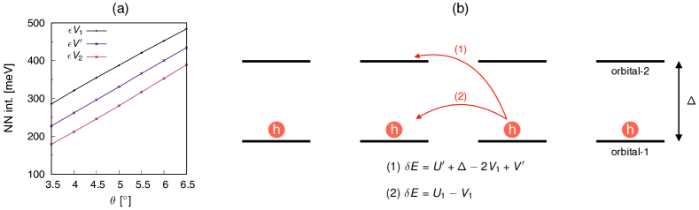
Figure S5: (a) The $\theta$-dependence of $V_{\eta}$ and $V^{\prime}$. (b) Schematic illustration of a one-dimensional two-orbital chain at one-hole filling ($n=1$). (1) and (2) highlight two different charge excitation processes with corresponding excitation energies, $\delta E=U^{\prime}+\Delta-2V_{1}+V^{\prime}$ and $\delta E=U_{1}-V_{1}$, respectively. We ignored $J$ for simplicity.

We now discuss qualitatively the effect of $V_{\eta\eta^{\prime}}$ for charge excitations. In Figure S5(b), we depict two different charge excitation processes denoted by (1) and (2) for a one-dimensional two-orbital chain at one-hole filling ($n=1$). The process-(1) corresponds to the charge-transfer (CT) excitation which leads to the triplet CT insulating phase in tWSe₂. On the other hand, the process-(2) depicts the single-orbital Mott-Hubbard excitation. From the explicit expression of the excitation energies, namely $\delta E=U^{\prime}+\Delta-2V_{1}+V^{\prime}$ for (1) and $\delta E=U_{1}-V_{1}$ for (2), it is clear that the effect of $V_{\eta\eta^{\prime}}$ is to promote the CT process rather than the Mott-Hubbard one because $V_{1}>V^{\prime}$ as shown in Figure S5(a). In certain experiments, this effect of intersite interactions may be less pronounced due to the external screening, e.g. by metallic gate, which is more effective for the intersite interactions than the onsite ones.

S9 Mott-Hubbard versus Hund physics on the transport scattering rate

S9.1 Why is Hund physics (not Mott-Hubbard) essential for the large resistance near $n=2$?

To understand the relationship between Hund physics and the large scattering rate (large resistance) near $n=2$, we performed the DMFT calculations with three different values of onsite energy level splitting $\Delta$, while keeping all the interaction parameters unchanged.

Figures S6(a–c) present our DMFT results for (a) $\Delta=\Delta_{\theta=4.2^{\circ}}$, (b) $\Delta=1.3\Delta_{\theta=4.2^{\circ}}$, and (c) $\Delta=1.5\Delta_{\theta=4.2^{\circ}}$. Here, $\Delta_{\theta=4.2^{\circ}}$ refers to the original value of onsite energy level splitting at $\theta=4.2^{\circ}$ of the system, which we obtained from the continuum-model band structure and was used for Figure 4b in the main text. Thus, Figure S6(a) is the same results as shown in Figure 4b.

By looking at Figures S6(a–c), one can clearly notice that a large transport scattering rate $(\Gamma/Z)_{\eta}$ near $n=2$ is realized for large $P_{1}$ and small $P_{0}$. Here $P_{S}$ is the probability of a given spin $S$ to be realized in the local two-hole subspace. In other words, the large resistance is attributed to the predominance of triplet ($S=1$) over singlet ($S=0$), which is promoted by Hund physics. This is because a large local spin moment impedes the formation of long-lived quasiparticles by protracting the Kondo screening of it Nevidomskyy ; Georges . It thus results in the degradation of conductivity because of strong scattering due to the unscreened local spin moment. On the contrary, Mott-Hubbard physics favors singlet rather than triplet formation for $n\lessapprox 1.9$ and gives rise to reduced scattering rate around $n=2$, even though a correlated insulator occurs at $n=1$ [Figure S6(c)].

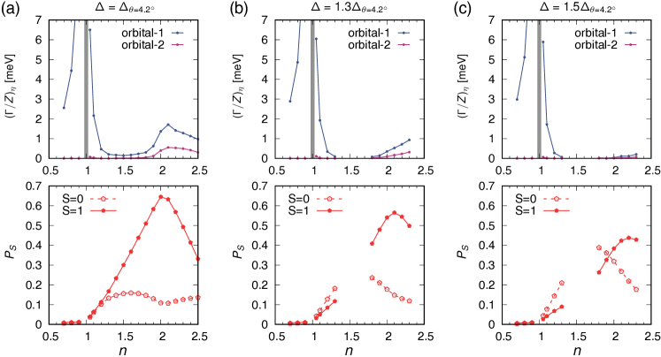
Figure S6: (a–c) The transport scattering rate (upper panels) and $P_{S}$ (lower panels) at $\theta=4.2^{\circ}$ and $\epsilon=8$. Three different values of onsite energy level splitting $\Delta$ were used for the same interaction parameters; (a) its orginal value $\Delta_{\theta=4.2^{\circ}}$, (b) 1.5$\Delta_{\theta=4.2^{\circ}}$, and (c) 1.7$\Delta_{\theta=4.2^{\circ}}$. The vertical gray bars at $n=1$ indicate correlated insulating phases.

S9.2 How does charge-transfer + Hund physics give rise to the resistance “peak” near $n=2$?

The analysis above indeed shows that Hund physics gives rise to the large resistance near $n=2$. However, one may also ask why the resistance “peak” rather than the value itself is related to Hund physics as well. The reason is closely related to orbital occupations. At one-hole filling ($n=1$), the occupation of orbtial-1 ($n_{1}$) and orbtial-2 ($n_{2}$) will be $n_{1}=1$ and $n_{0}=0$, as we have seen in Figure 3c and 3d in the main text. Then, let us assume a situation of $U_{1}-U^{\prime}\gg\Delta$ with a finite $J$. Here, $U_{1}$ is the intraorbital Coulomb repulsion of orbial-1 and $U^{\prime}$ the interorbital Coulomb repulsion. In this case, doped holes for $n>1$ will go to orbital-2 in order to minimize the Coulomb energy cost and to maximize the energy gain by Hund exchange. Thus, eventually at two-hole filling ($n=2$), orbital-1 and orbital-2 will be evenly occupied, i.e., $n_{1}=n_{2}=1$ forming spin-triplet $S=1$; see also Figure 3d in the main text. Since we are dealing with the “two-orbital” system, the situation of $n_{1}=n_{2}=1$ corresponds to the global half-filling. In this commensurate filling, charge fluctuations require additional energy which prohibits charges from freely moving from site to site.

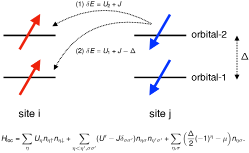
Figure S7: A two-orbital model at two-hole filling ($n=2$). The dotted arrows denote the low-energy charge excitations with energies $\delta E=U_{2}+J$ for (1) and $\delta E=U_{1}+J-\Delta$ for (2). The form of the local Hamiltonian $H_{\mathrm{loc}}$ is shown in the figure.

To further illustrate the above argument, see first Figure S7. Here, we focus on a two-orbital model at two-hole filling ($n=2$). The local part of Hamiltonian reads:

$$H_{\mathrm{loc}} =\sum_{\eta}U_{\eta}{n_{\eta\uparrow}n_{\eta\downarrow}}+\sum_{\eta<\eta^{\prime},\sigma\sigma^{\prime}}(U^{\prime}-J\delta_{\sigma\sigma^{\prime}}){n_{\eta\sigma}n_{\eta^{\prime}\sigma^{\prime}}}+\sum_{\eta,\sigma}\Big{(}\frac{\Delta}{2}(-1)^{\eta}-\mu\Big{)}n_{\eta\sigma},$$ (S7)

where $n_{i\eta\sigma}=d^{\dagger}_{i\eta\sigma}d_{i\eta\sigma}$ is the hole number operator. $\mu$ is the chemical potential. $\eta,\eta^{\prime}\in\{1,2\}$ are the orbital indices and $\sigma,\sigma^{\prime}\in\{\uparrow,\downarrow\}$ the spin indices. For simplicity, we ignore any non-density-density interactions which are irrelevant for the current analysis. The two low-energy charge excitation processes, with energies $\delta E=U_{2}+J$ for (1) and $\delta E=U_{1}+J-\Delta$ for (2), are denoted in Figure S7 with the dotted arrows. Note that the large resistance should correspond to large $\delta E$. As $\delta E$ increases with $J$ (and decreases with $\Delta$ for process-2), it can be seen that large $J$ and small $\Delta$ are detrimental to “good” conductivity, which is consistent with what we have discussed thus far.

References

- (1) Lee, P. A., Nagaosa, N. & Wen, X.-G. Doping a Mott insulator: Physics of high-temperature superconductivity. Rev. Mod. Phys. 78, 17–85 (2006). URL https://link.aps.org/doi/10.1103/RevModPhys.78.17.
- (2) Arovas, D. P., Berg, E., Kivelson, S. A. & Raghu, S. The Hubbard model. Annual Review of Condensed Matter Physics 13, 239–274 (2022).
- (3) Imada, M., Fujimori, A. & Tokura, Y. Metal-insulator transitions. Rev. Mod. Phys. 70, 1039–1263 (1998). URL https://link.aps.org/doi/10.1103/RevModPhys.70.1039.
- (4) Phillips, P. Mottness. Annals of Physics 321, 1634–1650 (2006). URL https://www.sciencedirect.com/science/article/pii/S0003491606000765.
- (5) Georges, A., Medici, L. d. & Mravlje, J. Strong correlations from Hund’s coupling. Annual Review of Condensed Matter Physics 4, 137–178 (2013). URL https://doi.org/10.1146/annurev-conmatphys-020911-125045.
- (6) Haule, K. & Kotliar, G. Coherence–incoherence crossover in the normal state of iron oxypnictides and importance of ’s rule coupling. New Journal of Physics 11, 025021 – 025033 (2009). URL https://doi.org/10.1088%2F1367-2630%2F11%2F2%2F025021.
- (7) Mravlje, J. et al. Coherence-incoherence crossover and the mass-renormalization puzzles in . Phys. Rev. Lett. 106, 096401 – 096404 (2011). URL https://link.aps.org/doi/10.1103/PhysRevLett.106.096401.
- (8) Yin, Z. P., Haule, K. & Kotliar, G. Kinetic frustration and the nature of the magnetic and paramagnetic states in iron pnictides and iron chalcogenides. Nature Materials 10, 932–935 (2011). URL https://doi.org/10.1038/nmat3120.
- (9) de’ Medici, L., Giovannetti, G. & Capone, M. Selective physics as a key to iron superconductors. Phys. Rev. Lett. 112, 177001 – 177005 (2014). URL https://link.aps.org/doi/10.1103/PhysRevLett.112.177001.
- (10) de’ Medici, L. Hund’s induced -liquid instabilities and enhanced quasiparticle interactions. Phys. Rev. Lett. 118, 167003 – 167007 (2017). URL https://link.aps.org/doi/10.1103/PhysRevLett.118.167003.
- (11) Fanfarillo, L., Valli, A. & Capone, M. Synergy between Hund-driven correlations and boson-mediated superconductivity. Phys. Rev. Lett. 125, 177001 (2020). URL https://link.aps.org/doi/10.1103/PhysRevLett.125.177001.
- (12) Miao, H. et al. Hund’s superconductor Li(Fe,Co)As. Phys. Rev. B 103, 054503 (2021). URL https://link.aps.org/doi/10.1103/PhysRevB.103.054503.
- (13) Lee, H. J., Kim, C. H. & Go, A. Hund’s metallicity enhanced by a van hove singularity in cubic perovskite systems. Phys. Rev. B 104, 165138 (2021). URL https://link.aps.org/doi/10.1103/PhysRevB.104.165138.
- (14) Fernandes, R. M. et al. Iron pnictides and chalcogenides: a new paradigm for superconductivity. Nature 601, 35–44 (2022).
- (15) Nevidomskyy, A. H. & Coleman, P. Kondo resonance narrowing in - and -electron systems. Phys. Rev. Lett. 103, 147205 (2009). URL https://link.aps.org/doi/10.1103/PhysRevLett.103.147205.
- (16) Yin, Z. P., Haule, K. & Kotliar, G. Fractional power-law behavior and its origin in iron-chalcogenide and ruthenate superconductors: Insights from first-principles calculations. Phys. Rev. B 86, 195141 – 195149 (2012). URL https://link.aps.org/doi/10.1103/PhysRevB.86.195141.
- (17) Aron, C. & Kotliar, G. Analytic theory of ’s metals: a renormalization group perspective. Phys. Rev. B 91, 041110(R) (2015). URL https://link.aps.org/doi/10.1103/PhysRevB.91.041110.
- (18) Stadler, K. M., Yin, Z. P., von Delft, J., Kotliar, G. & Weichselbaum, A. Dynamical mean-field theory plus numerical renormalization-group study of spin-orbital separation in a three-band metal. Phys. Rev. Lett. 115, 136401 – 136405 (2015). URL https://link.aps.org/doi/10.1103/PhysRevLett.115.136401.
- (19) Horvat, A., Žitko, R. & Mravlje, J. Low-energy physics of three-orbital impurity model with interaction. Phys. Rev. B 94, 165140 – 165150 (2016). URL https://link.aps.org/doi/10.1103/PhysRevB.94.165140.
- (20) Drouin-Touchette, V., König, E. J., Komijani, Y. & Coleman, P. Emergent moments in a Hund’s impurity. Phys. Rev. B 103, 205147 (2021). URL https://link.aps.org/doi/10.1103/PhysRevB.103.205147.
- (21) Hoshino, S. & Werner, P. Superconductivity from emerging magnetic moments. Phys. Rev. Lett. 115, 247001 – 247005 (2015). URL https://link.aps.org/doi/10.1103/PhysRevLett.115.247001.
- (22) Vafek, O. & Chubukov, A. V. Hund interaction, spin-orbit coupling, and the mechanism of superconductivity in strongly hole-doped iron pnictides. Phys. Rev. Lett. 118, 087003 (2017). URL https://link.aps.org/doi/10.1103/PhysRevLett.118.087003.
- (23) Coleman, P., Komijani, Y. & König, E. J. Triplet resonating valence bond state and superconductivity in Hund’s metals. Phys. Rev. Lett. 125, 077001 (2020). URL https://link.aps.org/doi/10.1103/PhysRevLett.125.077001.
- (24) Isidori, A. et al. Charge disproportionation, mixed valence, and effect in multiorbital systems: A tale of two insulators. Phys. Rev. Lett. 122, 186401 – 186406 (2019). URL https://link.aps.org/doi/10.1103/PhysRevLett.122.186401.
- (25) Ryee, S., Sémon, P., Han, M. J. & Choi, S. Nonlocal Coulomb interaction and spin-freezing crossover as a route to valence-skipping charge order. npj Quantum Materials 5, 19 (2020). URL https://doi.org/10.1038/s41535-020-0221-9.
- (26) Ryee, S., Han, M. J. & Choi, S. Hund physics landscape of two-orbital systems. Phys. Rev. Lett. 126, 206401 (2021). URL https://link.aps.org/doi/10.1103/PhysRevLett.126.206401.
- (27) Kuneš, J. & Augustinský, P. Excitonic instability at the spin-state transition in the two-band Hubbard model. Phys. Rev. B 89, 115134 (2014). URL https://link.aps.org/doi/10.1103/PhysRevB.89.115134.
- (28) Geffroy, D. et al. Collective modes in excitonic magnets: Dynamical mean-field study. Phys. Rev. Lett. 122, 127601 (2019). URL https://link.aps.org/doi/10.1103/PhysRevLett.122.127601.
- (29) Werner, P. & Murakami, Y. Nonthermal excitonic condensation near a spin-state transition. Phys. Rev. B 102, 241103 (2020). URL https://link.aps.org/doi/10.1103/PhysRevB.102.241103.
- (30) Ryee, S., Choi, S. & Han, M. J. Frozen spin ratio and the detection of Hund correlations. arXiv preprint arXiv:2207.10421 (2022). URL https://arxiv.org/abs/2207.10421.
- (31) Kennes, D. M. et al. Moiréheterostructures as a condensed-matter quantum simulator. Nature Physics 17, 155–163 (2021).
- (32) Georges, A. & Kotliar, G. Hubbard model in infinite dimensions. Phys. Rev. B 45, 6479–6483 (1992). URL https://link.aps.org/doi/10.1103/PhysRevB.45.6479.
- (33) Scuri, G. et al. Electrically tunable valley dynamics in twisted bilayers. Phys. Rev. Lett. 124, 217403 (2020). URL https://link.aps.org/doi/10.1103/PhysRevLett.124.217403.
- (34) Wang, L. et al. Correlated electronic phases in twisted bilayer transition metal dichalcogenides. Nature Materials 19, 861–866 (2020). URL https://doi.org/10.1038/s41563-020-0708-6.
- (35) Zhang, Z. et al. Flat bands in twisted bilayer transition metal dichalcogenides. Nature Physics 16, 1093–1096 (2020).
- (36) Andersen, T. I. et al. Excitons in a reconstructed moirépotential in twisted WSe2/WSe2 homobilayers. Nature Materials 20, 480–487 (2021). URL https://doi.org/10.1038/s41563-020-00873-5.
- (37) Ghiotto, A. et al. Quantum criticality in twisted transition metal dichalcogenides. Nature 597, 345–349 (2021). URL https://doi.org/10.1038/s41586-021-03815-6.
- (38) Xu, Y. et al. A tunable bilayer hubbard model in twisted WSe2. Nature Nanotechnology (2022).
- (39) Wu, F., Lovorn, T., Tutuc, E. & MacDonald, A. H. Hubbard model physics in transition metal dichalcogenide moiré bands. Phys. Rev. Lett. 121, 026402 (2018). URL https://link.aps.org/doi/10.1103/PhysRevLett.121.026402.
- (40) Lopes dos Santos, J. M. B., Peres, N. M. R. & Castro Neto, A. H. Graphene bilayer with a twist: Electronic structure. Phys. Rev. Lett. 99, 256802 (2007). URL https://link.aps.org/doi/10.1103/PhysRevLett.99.256802.
- (41) Bistritzer, R. & MacDonald, A. H. Moiré bands in twisted double-layer graphene. Proceedings of the National Academy of Sciences 108, 12233–12237 (2011). URL https://www.pnas.org/doi/abs/10.1073/pnas.1108174108.
- (42) Pan, H., Wu, F. & Das Sarma, S. Band topology, Hubbard model, Heisenberg model, and Ezyaloshinskii-Moriya interaction in twisted bilayer . Phys. Rev. Research 2, 033087 (2020). URL https://link.aps.org/doi/10.1103/PhysRevResearch.2.033087.
- (43) Devakul, T., Crépel, V., Zhang, Y. & Fu, L. Magic in twisted transition metal dichalcogenide bilayers. Nature Communications 12, 6730 (2021). URL https://doi.org/10.1038/s41467-021-27042-9.
- (44) Georges, A., Kotliar, G., Krauth, W. & Rozenberg, M. J. Dynamical mean-field theory of strongly correlated fermion systems and the limit of infinite dimensions. Rev. Mod. Phys. 68, 13–125 (1996). URL https://link.aps.org/doi/10.1103/RevModPhys.68.13.
- (45) Zang, J., Wang, J., Cano, J. & Millis, A. J. Hartree-Fock study of the moiré hubbard model for twisted bilayer transition metal dichalcogenides. Phys. Rev. B 104, 075150 (2021). URL https://link.aps.org/doi/10.1103/PhysRevB.104.075150.
- (46) Zang, J., Wang, J., Cano, J., Georges, A. & Millis, A. J. Dynamical mean-field theory of moiré bilayer transition metal dichalcogenides: Phase diagram, resistivity, and quantum criticality. Phys. Rev. X 12, 021064 (2022). URL https://link.aps.org/doi/10.1103/PhysRevX.12.021064.
- (47) Wietek, A. et al. Tunable stripe order and weak superconductivity in the moiré Hubbard model. Phys. Rev. Research 4, 043048 (2022). URL https://link.aps.org/doi/10.1103/PhysRevResearch.4.043048.
- (48) Klebl, L., Fischer, A., Classen, L., Scherer, M. M. & Kennes, D. M. Competition of density waves and superconductivity in twisted tungsten diselenide. arXiv preprint arXiv:2204.00648 (2022). URL https://arxiv.org/abs/2204.00648.
- (49) Wu, Y.-M., Wu, Z. & Yao, H. Pair-density-wave and chiral superconductivity in twisted bilayer transition-metal-dichalcogenides. arXiv preprint arXiv:2203.05480 (2022). URL https://arxiv.org/abs/2203.05480.
- (50) Bélanger, M., Fournier, J. & Sénéchal, D. Superconductivity in the twisted bilayer transition metal dichalcogenide : A quantum cluster study. Phys. Rev. B 106, 235135 (2022). URL https://link.aps.org/doi/10.1103/PhysRevB.106.235135.
- (51) Zaanen, J., Sawatzky, G. A. & Allen, J. W. Band gaps and electronic structure of transition-metal compounds. Phys. Rev. Lett. 55, 418–421 (1985). URL https://link.aps.org/doi/10.1103/PhysRevLett.55.418.
- (52) Zhang, F. C. & Rice, T. M. Effective Hamiltonian for the superconducting Cu oxides. Phys. Rev. B 37, 3759–3761 (1988). URL https://link.aps.org/doi/10.1103/PhysRevB.37.3759.
- (53) Springer, D. et al. Osmates on the verge of a Hund’s-Mott transition: The different fates of and . Phys. Rev. Lett. 125, 166402 (2020). URL https://link.aps.org/doi/10.1103/PhysRevLett.125.166402.
- (54) Laturia, A., Van de Put, M. L. & Vandenberghe, W. G. Dielectric properties of hexagonal boron nitride and transition metal dichalcogenides: from monolayer to bulk. npj 2D Materials and Applications 2, 6 (2018). URL https://doi.org/10.1038/s41699-018-0050-x.
- (55) Yu, G., Wen, L., Luo, G. & Wang, Y. Band structures and topological properties of twisted bilayer MoTe2 and WSe2. Physica Scripta 96, 125874 (2021). URL https://doi.org/10.1088/1402-4896/ac4192.
- (56) Zhang, Y., Yuan, N. F. Q. & Fu, L. Moiré quantum chemistry: Charge transfer in transition metal dichalcogenide superlattices. Phys. Rev. B 102, 201115(R) (2020). URL https://link.aps.org/doi/10.1103/PhysRevB.102.201115.
- (57) Wu, F., Lovorn, T., Tutuc, E., Martin, I. & MacDonald, A. H. Topological insulators in twisted transition metal dichalcogenide homobilayers. Phys. Rev. Lett. 122, 086402 (2019). URL https://link.aps.org/doi/10.1103/PhysRevLett.122.086402.
- (58) Witt, N. et al. Doping fingerprints of spin and lattice fluctuations in moiré superlattice systems. Phys. Rev. B 105, L241109 (2022). URL https://link.aps.org/doi/10.1103/PhysRevB.105.L241109.
- (59) Marzari, N., Mostofi, A. A., Yates, J. R., Souza, I. & Vanderbilt, D. Maximally localized wannier functions: Theory and applications. Rev. Mod. Phys. 84, 1419–1475 (2012). URL https://link.aps.org/doi/10.1103/RevModPhys.84.1419.
- (60) Pizarro, J. M., Rösner, M., Thomale, R., Valentí, R. & Wehling, T. O. Internal screening and dielectric engineering in magic-angle twisted bilayer graphene. Phys. Rev. B 100, 161102(R) (2019). URL https://link.aps.org/doi/10.1103/PhysRevB.100.161102.
- (61) Steinke, C., Wehling, T. O. & Rösner, M. Coulomb-engineered heterojunctions and dynamical screening in transition metal dichalcogenide monolayers. Phys. Rev. B 102, 115111 (2020). URL https://link.aps.org/doi/10.1103/PhysRevB.102.115111.
- (62) van Loon, E. G. et al. Coulomb engineering of two-dimensional mott materials. arXiv preprint arXiv:2001.01735 (2020). URL https://arxiv.org/abs/2001.01735.
- (63) Cudazzo, P., Tokatly, I. V. & Rubio, A. Dielectric screening in two-dimensional insulators: Implications for excitonic and impurity states in graphane. Phys. Rev. B 84, 085406 (2011). URL https://link.aps.org/doi/10.1103/PhysRevB.84.085406.
- (64) Berkelbach, T. C., Hybertsen, M. S. & Reichman, D. R. Theory of neutral and charged excitons in monolayer transition metal dichalcogenides. Phys. Rev. B 88, 045318 (2013). URL https://link.aps.org/doi/10.1103/PhysRevB.88.045318.
- (65) Kylänpää, I. & Komsa, H.-P. Binding energies of exciton complexes in transition metal dichalcogenide monolayers and effect of dielectric environment. Phys. Rev. B 92, 205418 (2015). URL https://link.aps.org/doi/10.1103/PhysRevB.92.205418.
- (66) Gull, E. et al. Continuous-time methods for quantum impurity models. Rev. Mod. Phys. 83, 349 – 404 (2011). URL https://link.aps.org/doi/10.1103/RevModPhys.83.349.
- (67) Choi, S., Semon, P., Kang, B., Kutepov, A. & Kotliar, G. Comdmft: A massively parallel computer package for the electronic structure of correlated-electron systems. Computer Physics Communications 244, 277–294 (2019). URL https://www.sciencedirect.com/science/article/pii/S0010465519302140.
- (68) Jarrell, M. & Gubernatis, J. Bayesian inference and the analytic continuation of imaginary-time quantum monte carlo data. Physics Reports 269, 133–195 (1996). URL https://www.sciencedirect.com/science/article/pii/0370157395000747.
- (69) Bergeron, D. & Tremblay, A.-M. S. Algorithms for optimized maximum entropy and diagnostic tools for analytic continuation. Phys. Rev. E 94, 023303 (2016). URL http://link.aps.org/doi/10.1103/PhysRevE.94.023303.