An Effective Approach for Multi-label Classification with Missing Labels

Abstract

Compared with multi-class classification, multi-label classification that contains more than one class is more suitable in real life scenarios. Obtaining fully labeled high-quality datasets for multi-label classification problems, however, is extremely expensive, and sometimes even infeasible, with respect to annotation efforts, especially when the label spaces are too large. This motivates the research on partial-label classification, where only a limited number of labels are annotated and the others are missing. To address this problem, we first propose a pseudo-label based approach to reduce the cost of annotation without bringing additional complexity to the existing classification networks. Then we quantitatively study the impact of missing labels on the performance of classifier. Furthermore, by designing a novel loss function, we are able to relax the requirement that each instance must contain at least one positive label, which is commonly used in most existing approaches. Through comprehensive experiments on three large-scale multi-label image datasets, i.e. MS-COCO, NUS-WIDE, and Pascal VOC12, we show that our method can handle the imbalance between positive labels and negative labels, while still outperforming existing missing-label learning approaches in most cases, and in some cases even approaches with fully labeled datasets.

I Introduction

In deep learning, multi-class classification is a common problem where the goal is to classify a set of instances, each associated with a unique class label from a set of disjoint class labels. A generalized version of multi-class problem is multi-label classification [1], which allows the instances to be associated with more than one class. It is more a practical problem in real life because of the intrinsic multi-label property of the physical world [2]: automatic driving always needs to identify which objects are contained in the current scene, such as cars, traffic lights and pedestrians; CT scan can detect a variety of possible lesions; a movie can simultaneously belong to different categories, for instance. Ideally, multi-label classification is a form of supervised learning [3], which requires lots of accurate labels. In practice, however, annotating all labels for each training instance raises a great challenge in multi-label classification, which is time-consuming and even impractical especially in the presence of a large number of categories [4, 5]. Therefore, how to leverage the performance of multi-label classifier and the cost of collecting labels receives significant interests in recent years.

The main strategies can be roughly divided into two categories: (1) generating annotations automatically and (2) training with missing labels. The former uses the web as the supervisor to generate annotations [6, 7, 8], since there is a large amount of imagery data with labeled information available on the web, such as social media hashtags and connections between web-pages and user feedback. However, these methods may introduce additional noises to the label space, which can degrade a classifier’s performance. For the latter, missing labels means that only a subset of all the labels can be observed and the rest remains unknown. It can be further divided into several representative settings: fully observed labels (FOL), partially observed labels (POL), which is the most common setting. Two variations of POL include: partially observed positive labels (PPL) and single positive label (SPL). Table I shows the difference between these settings. It should be pointed out that POL setting is more common than PPL in real life. For example, in many execution records of industrial devices [9, 10, 11], the probability of each component’s failure is extremely low. Therefore, it is almost impossible to guarantee that each instance corresponds to one positive label, let alone in the setting of missing labels.

TABLE I: Different Missing-label Settings. ✓, $\times$, $\varnothing$ represent that current instance belongs to this class, does not belong to this class, and lacks related label, respectively.

Settings	Class 1	Class 2	Class 3	Class 4	Class 5
FOL	✓	$\times$	✓	$\times$	✓
POL	✓	$\varnothing$	$\varnothing$	$\times$	✓
PPL	✓	$\varnothing$	✓	$\varnothing$	$\varnothing$
SPL	✓	$\varnothing$	$\varnothing$	$\varnothing$	$\varnothing$

This paper focuses on multi-label classification with missing labels. Although there has been a lot of work done along this direction [5, 12], there are still some critical issues to be addressed:

• To solve the multi-label classification with missing labels, many state-of-the-art (SOTA) methods [2][4] rely on additional structures, such as GNN and label estimator, which further increase the complexity of networks. A natural question is whether this problem can be effectively solved without significantly increasing the network complexity.

• It is still not clear how the missing ratio of the labels affects the classification performance, which is of great importance for us to balance the performance of classifier and the annotation cost.

• Due to imbalance between positive and negative labels, most methods dealing with missing labels require that there is at least one positive label per instance, i.e., PPL, instead of POL, which is more common in real life.

With these observations, this paper investigates new approaches for multi-label classification with missing labels. The main contributions are summarized as follows:

• We propose a pseudo-label-based approach to predict all possible categories with missing labels, which can effectively balance the performance of classifiers and the cost of annotation. The network structure in our approach is the same as the classifier trained with full labels, which means that our approach will not increase the network complexity. The major difference lies in the novel design of loss functions and training schemes.

• We provide systematical and quantitative analysis of the impact of labels’ missing ratio on the classifier’s performance. In particular, we relax the strict requirement that the label space of each instance must contain at least one positive label, which is commonly seen in the related work [4, 5]. Therefore, our method is applicable to general POL settings, not only PPL.

• Comprehensive experiments verify that our approach can be effectively applied to missing-label classification. Specifically, our approach outperforms most existing missing-label learning approaches, and in some cases even approaches trained with fully labeled datasets. More importantly, our approach can adopt POL settings, which is incompatible with most existing methods.

The rest of the paper is organized as follows. Section II discusses the related work. The problem is formulated in Section III and our proposed method is presented in Section IV. Section V shows the experimental results. Finally, conclusions are drawn in Section VI.

II Related Work

II-A Multi-label Learning with Missing Labels

Recently, numerous methods have been proposed for multi-label classification with missing labels. Herein, we briefly review the relevant studies.

Binary Relevance (BR). A straightforward approach for multi-label learning with missing labels is BR [1, 13], which decomposes the task into a number of binary classification problems, each for one label. Such an approach encounters many difficulties, mainly due to ignoring correlations between labels. To address this issue, many correlation-enabling extensions to binary relevance have been proposed [14, 12, 15, 16, 17]. However, most of these methods require solving an optimization problem while keeping the training set in memory at the same time. So it is extremely hard, if not impossible, to apply a mini-batch strategy to fine-tune the model [2], which will limit the use of pre-trained neural networks (NN) [18].

Positive and Unlabeled Learning (PU-learning). PU-learning is an alternative solution [19], which studies the problem with a small number of positive examples and a large number of unlabeled examples for training. Most methods can be divided into the following three categories: two-step techniques [20, 21, 22], biased learning [23, 24], and class prior incorporation [25, 26]. All these methods require that the training data consists of positive and unlabeled examples [27]. In other words, they treat the negative labels as unlabeled, which discard the existing negatives and does not make full use of existing labels.

Pseudo Label. Pseudo-labeling was first proposed in [28]. The goal of pseudo-labeling is to generate pseudo-labels for unlabeled samples [29]. There are different methods to generate pseudo labels: the work in [28, 30] uses the predictions of a trained NN to assign pseudo labels. Neighborhood graphs are used in [31]. The approach in [32] updates pseudo labels through an optimization framework. It is worth mentioning that MixMatch-family semi-supervised learning methods [33, 34, 35, 36] achieve SOTA on multi-class problem by utilizing pseudo labels and consistency regularization [37]. However, creation of negative pseudo-labels (i.e. labels which specify the absence of specific classes) is not supported by these methods, which therefore affects the performance of classifier by neglecting negative labels [30]. Instead, the work in [30] obtains the reference values of pseudo labels directly from the network predictions and then generates hard pseudo labels by setting confidence thresholds for positive and negative labels, respectively. Different from [30], we simplify this process by studying the proportion of positive and negative labels to generate pseudo labels.

II-B Imbalance

A key characteristic of multi-label classification is the inherent positive-negative imbalance created when the overall number of labels is large [38]. Missing labels exacerbate the imbalance and plague recognizing positives [5]. Therefore, the work in [5, 4] mandates that each instance in the training set must have at least one positive label, which means that they focus on PPL setting instead of “real” POL. Obviously, this assumption may not always hold in real life scenarios. To relax this assumption, a trivial solution is to treat the instances with only negative labels as unlabeled instances. In this case, however, it wastes the value of negative labels.

In this work, we allow the instances in training sets with only negative labels (that is POL setting). From this perspective, our work is most closely related to [2]. It should be pointed out that [2] uses a Graph Neural Network (GNN) [39] on top of a Convolutional Neural Network (CNN) to model the correlations between labels, and its message update function relies on a multi-layer perception (MLP), which brings extra additional complexity to the parameter space and training process. Whereas our approach focuses on designing the training schemes and the loss function without introducing additional structures. Furthermore, although [2] can cope with instances containing only negative labels, it does not specifically explore this direction, which leaves the possibility of falling into a trivial solution (always predict negative) when these types of instances occupies the majority.

III Formulation

III-A Multi-label Classification

Given a multi-label classifier with full labels, let $\mathcal{X}=\mathbb{R}^{M}$ be the input attribute space of $M$-dimensional feature vectors and $\mathcal{Y}=\{1,2,\ldots,L\}$ denote the set of $L$ possible labels. An instance $\textbf{x}\in\mathcal{X}$ is associated with a subset of labels $\textbf{y}\in 2^{\mathcal{Y}}$, which can be represented as an $L$-vector $\textbf{y}=[y_{1},y_{2},\ldots,y_{L}]=\{0,1\}^{L}$ where $y_{j}=1$ iff the $j$th label is relevant (otherwise $y_{j}=0$). Let $\mathcal{D}=\{(\textbf{x}_{1},\textbf{y}_{1}),\ldots,(\textbf{x}_{N},\textbf{y}_{N})\}$ is the training set of $N$ samples. Given $\mathcal{D}$, a multi-label classifier $h:\mathcal{X}\rightarrow\mathcal{Y}$ learns to map the attribute input space to the label output space. We use $\hat{\textbf{y}}$ to present the prediction of classifier $h$, that is, $\hat{\textbf{y}}=f(h(\textbf{x}))$, where $f(\cdot)$ stands for a function (commonly the sigmoid function as $\sigma(s)=\frac{1}{1+e^{-s}}$) that turns confidence outputs into a prediction. In this case, most of the existing work [40, 1, 41, 42] adopts the binary cross entropy (BCE) function as the loss function, which is formulated by

$$\mathcal{L}(\hat{y},y)=-\frac{1}{L}\sum_{i=1}^{L}[(y_{i}\log(\hat{y}_{i})+(1-y_{i})\log(1-\hat{y}_{i})].$$ (1)

For multi-label classification with missing-label, we use $\textbf{z}=[z_{1},z_{2},\ldots,z_{L}]=\{0,1,\varnothing\}^{L}$ to present the observed labels, where $z_{j}=\varnothing$ means the corresponding label is missing. It is worth mentioning that the training set is $\mathcal{D}=\{(\textbf{x}_{1},\textbf{z}_{1}),\ldots,(\textbf{x}_{N},\textbf{z}_{N})\}$, while validation and test set is $\mathcal{D}_{v}=\mathcal{D}_{t}=\{(\textbf{x}_{1},\textbf{y}_{1}),\ldots,(\textbf{x}_{N},\textbf{y}_{N})\}$ in this case. In other words, we still use full labels for validation and testing.

III-B Different Missing-label Settings

According to the number and positive/negative properties of the observable labels, we divide multi-label classification problem into several settings: partially observed labels (POL), partially positive labels (PPL), and an extreme case, i.e., single positive label (SPL) [4]. Specially, we formulate these settings as the following:

$$\textbf{z}_{POL}=\{0,1,\varnothing\}^{L}\text{ and }$$ (2)

$$\sum_{j=1}^{L}(\mathbf{1}_{[\textbf{z}_{POL_{j}}=1]}+\mathbf{1}_{[\textbf{z}_{POL_{j}}=0]})<L,$$

$$\textbf{z}_{PPL}=\{1,\varnothing\}^{L}\text{ and }\sum_{j=1}^{L}\mathbf{1}_{[\textbf{z}_{PPL_{j}}=1]}<L,$$ (3)

$$\textbf{z}_{SPL}=\{1,\varnothing\}^{L}\text{ and }\sum_{j=1}^{L}\mathbf{1}_{[\textbf{z}_{PPL_{j}}=1]}=1,$$ (4)

where $\mathbf{1}_{[\cdot]}$ stands for the indicator function, that is, $\mathbf{1}_{[True]}=1$ and $\mathbf{1}_{[False]}=0$. Considering the large number of unknown labels and the imbalance problem in these settings, we design a new loss function to handle them, instead of directly using BCE (1).

IV Proposed Method

Without changing the basic structure of the classification network, we address multi-label classification with missing labels by introducing pseudo-label, designing new loss functions, and adjusting training schemes. The pipeline of our method is shown as Fig. 1.

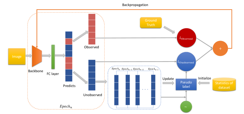
Figure 1: Pipeline of our method. We feed an image to the classifier network and obtain the predictions. Then different strategies are utilized to deal with observed and unobserved labels. For the unobserved part, we introduce pseudo labels by leveraging the prior knowledge of the dataset and design a novel loss function $\mathcal{L}_{\text{Unobserved}}$. For the observed part, we treat it as a full-label classification problem. The total loss is defined by adding the losses of these two parts with designed weights. The network used in our method is the most common classification network, which means that there is no additional complexity in the network structure.

IV-A Pseudo-labels

For all missing-label settings, the label of any instance in the training set can be divided into two categories: observed and unobserved labels. [43, 44, 45] directly set the unobserved labels as negative. However, performance drops because a lot of ground-truth positive labels are initialized as negatives [46]. Therefore, we decide to introduce soft pseudo labels for the unobserved part and take pseudo labels as the target value of unobserved labels in calculation of the loss. Another benefit of introducing pseudo labels is that by properly designing updating methods, it will not add complexity to the existing classifier network. In contrast, ROLE [4] adds another NN as the label estimator and takes the predictions of this NN as the target. [2] adds a GNN on top of a CNN. Obviously, these methods bring additional complexity to the network.

In our approach, the classifier actually has two goals in the training process:

• For observed labels, we expect the predicted value to be pushed to its ground-true value.

• For unobserved labels, we expect the predicted value to be as close as possible to the value of its corresponding pseudo label.

All the design steps in our method revolve these two points. For (1), we just need to do as traditional supervised learning does. For (2), there are two issues in front of us, that is, how to generate pseudo-labels and how to update them. In the following discussion, we denote pseudo labels as $\widetilde{\textbf{y}}$ and the pseudo-labeling value corresponding to the $i$th instance’s $j$th class as $\widetilde{y}_{i_{j}}$, which can be any real number between $[0,1]$.

Creation of Pseudo-labels. There are several approaches to create pseudo-labels for unobserved labels, as described in Section II. In this work, we simplify this step by leveraging the prior knowledge of the datasets. We first calculate the average number of observed positive labels per instance and denote it as $P_{p}$, and then count the missing ratio $m$ of the current training set, $m=T_{o}/T$, where $T_{o}$ and $T$ stand for the number of observed and total labels, respectively. We expect that $P_{p}/m$ can, to some extent, approximate or recover the average number of positive labels per instance over the entire dataset. With these statistics about the missing-label dataset, we can set the initial value for pseudo labels of the $i$th instance $\widetilde{y}_{i_{j}}$ as

$$\widetilde{y}_{i_{j}}=\begin{cases}\min\left(\frac{\max(\frac{P_{p}}{m},1)-P_{i}}{T_{u_{i}}},1\right),&\max(\frac{P_{p}}{m},1)>P_{i}\\ 0,&\textit{otherwise}\end{cases}$$ (5)

for unobserved label $j$, where $P_{i}$ and $T_{u_{i}}$ stand for the number of the observed positive labels and unobserved labels in the $i$th instance, respectively. By using the $\max$ function in (5), it means we have an initial guess that each instance has at least one positive label in average, either observed or unobserved (of course, such an initial guess is not necessarily true).

The initial method relies on a fact that even though most of the labels are missing, the statistics of the observed labels can still be used as a reference for the overall distribution of this dataset. Therefore, if the number of an instance’s observed positive labels, $P_{i}$, is less than the average $\max(P_{p}/m,1)$, we assign the difference, divided by $T_{u_{i}}$, as the pseudo labels of those unobserved labels on this instance. Otherwise, if the number of the observed positive labels exceeds the average, we set the pseudo labels to 0. Note that this setting is only for initialization. The pseudo labels will be updated during the training progresses.

It is worth mentioning that the previous approaches often initialize the pseudo labels as 0.5 or 0. Compared with the 0.5 setting, they do not take full advantage of the statistic information of the dataset. As to the 0 setting, it may aggravate the label imbalance.

Update. We update the value of pseudo labels after each epoch of updating the network. A common way is to simply use the network predictions as the pseudo labels. To check the trajectory of the pseudo labels of this method, we randomly select 10 training instances and record the fluctuations of their predictions and pseudo labels’ value in SPL settings. Due to space limitation, we only show the fluctuations of one category of one instance in Fig. 2. Obviously, the predictions fluctuate greatly in this common update method (as shown in the left plot in Fig. 2). Note that even in the later stage of training, the fluctuation still exists, which makes it hard to converge. This is clearly not what we expect in training.

Therefore, we use a stack to record the predictions of our classifier for the past $n$ epochs and take the average of these historical predictions as the value for the associated pseudo labels, where $n$ is a hyperparameter. Following this method, we record the trajectories of the predictions and the pseudo labels on the same training instances under SPL setting during training (the right plot in Fig. 2). It is easy to find that this running-average method smooths the fluctuation of predictions and accelerate the convergence. We formulate this updating method as follows:

$$\widetilde{y}_{i_{j}}=\frac{1}{n}\sum_{k=0}^{n-1}\hat{y}_{i_{j}}^{m-k}$$ (6)

where $m$ stands for the current epoch index and $\hat{y}_{i_{j}}^{m}$ stands for the predicted value of the $j$th category in the $i$th instance at the $m$th epoch.

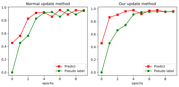
Figure 2: Fluctuations in predicted values and pseudo labels during training. The GT value for this specific label is 1. The left and right plot shows the trajectories of the predicted and pseudo labels under traditional updating method (set the pseudo label equal to the predicted value) and our running-average updating method, respectively. It is easy to see that our method accelerates convergence and smooths updating trajectories.

Disturbance Injection. In experiments, we find that the predictions of the classifier for some unobserved categories remain around 0.5. As mentioned before, we believe that it is always better for the classifier to give an answer instead of being ambiguities. Following this concept, we devise a detector to detect such vague decisions. By utilizing the historical prediction stack $S_{pse}=\{\hat{y}_{i_{j}}^{m-k}\}_{k=0}^{n-1}$, we determine whether these predictions are all in interval $[0.5-d,0.5+d]$, where $d$ is a hyperparameter. If so, we update the pseudo labels using (7), instead of updating pseudo labels in (6), which adds random disturbances to these kind of unobserved categories to push the pseudo labels away from 0.5:

$$\widetilde{y}_{i_{j}}=\begin{cases}\hat{y}_{i_{j}}-\text{random}(0,\hat{y}_{i_{j}}),&\hat{y}_{i_{j}}<0.5\\ \hat{y}_{i_{j}}+\text{random}(0,1-\hat{y}_{i_{j}}),&\text{otherwise}\end{cases}$$ (7)

where $\text{random}(a,b)$ stands for a function which generates a random real number between $a$ and $b$.

Algorithm 1 summarizes the updating process of pseudo labels. It should be pointed that the detection will not be performed in the first $D_{s}$ epochs and the last $D_{e}$ epochs of training, since the predicted labels may fall into $[0.5-d,0.5+d]$ simply due to non-convergence at the beginning of training and training may stop before reaching convergence in the last several epochs. Here $D_{s}$ and $D_{e}$ are also hyperparameters.

Algorithm 1 Update_pseudo()

0:  predcited value $\hat{y_{i_{j}}}$ for $j$th class of $i$th instance at epoch $m$, stack $\textbf{S}_{i_{j}}$, start epoch $D_{s}$, end epoch $D_{e}$

1:  if $D_{s}<m<D_{e}$  then

2:     if $\textbf{S}_{i_{j}}$ is FULL then

3:        $\textbf{S}_{i_{j}}$.pop()

4:     end if

5:     $\textbf{S}_{i_{j}}$.push($\hat{y_{i_{j}}}$)

6:     if detector($\textbf{S}_{i_{j}}$) is TRUE then

7:        update pseudo labels $\widetilde{y}_{i_{j}}$ based on (7)

8:     else

9:        $\widetilde{y}_{i_{j}}\leftarrow$ avg($\textbf{S}_{i_{j}}$) based on (6)

10:     end if

11:  end if

11:  $\widetilde{y}_{i_{j}}$, $\textbf{S}_{i_{j}}$

IV-B Design of Loss function

At this point, we have solutions to meet the two goals mentioned in Subsection IV-A. Next, we relate these two goals together by designing an appropriate loss function. Intuitively, we can obtain the loss function by adding the losses of the observed part and unobserved part:

$$\mathcal{L}=\mathcal{L}_{\text{Observed}}+\mathcal{L}_{\text{Unobserved}}$$ (8)

where $\mathcal{L}_{\text{Observed}}$ is obtained by modifying the number of classes $L$ in (1) to the number of observed labels $O_{i}$ in the $i$th instance:

$$\mathcal{L}_{\text{Observed}}=-\frac{1}{O_{i}}\sum_{j=1}^{O_{i}}[y_{j}\log(\hat{y}_{j})+(1-y_{j})\log(1-\hat{y}_{j})].$$ (9)

Before passing the pseudo labels into the loss function, we define a threshold function on the pseudo labels, $f(\widetilde{y_{i}},t)$, where $t$ is a hyperparameter. In order to simplify the description, this threshold is ignored below. For $\mathcal{L}_{\text{Unobserved}}$, since the pseudo labels may contain errors, we can generally regard them as the GT values with noises. Therefore, we follow the idea in [47] to design $\mathcal{L}_{\text{SBCE}}$ as follows, which has been proven to be robust to noises:

$$\mathcal{L}_{\text{Unobserved}}=\mathcal{L}_{\text{SBCE}}=\alpha\mathcal{L}(\hat{y},\widetilde{y})+\beta\mathcal{L}(\widetilde{y},\hat{y}).$$ (10)

where $\alpha$ and $\beta$ stand for two decoupled hyperparameters.

Imbalance between Positives and Negatives. Label imbalance significantly affects the generalization performance of the multi-label predictive model. The classifier can be easily reduced to the trivial “always predict positive/negative” solution. To alleviate imbalance, we add confidence scores into $\mathcal{L}_{\text{Unobserved}}$ to balance the contributions of positive and negatives during training:

$$\mathcal{L}_{\text{CFS}}(x,y,C_{1},C_{2},L)= -\frac{1}{L}\sum_{i=1}^{L}[C_{1}x_{i}\log(y_{i})$$ (11)

$$+C_{2}(1-x_{i})\log(1-y_{i})],$$

where $C_{1}=\frac{N}{T}$ and $C_{2}=\frac{P}{T}$ are the weights, $N$ and $P$ stand for the total number of the observed negative and positive labels, respectively, and $T=N+P$ stands for the total number of observed labels in the training set. Obviously, $C_{1}+C_{2}=1$. Accordingly, the loss function for unobserved part can be defined as follows:

$$\mathcal{L}_{\text{Unobserved}}= \alpha\mathcal{L}_{\text{CFS}}(\hat{y},\widetilde{y},C_{1},C_{2},U)$$ (12)

$$+\beta\mathcal{L}_{\text{CFS}}(\widetilde{y},\hat{y},C_{1},C_{2},U),$$

where $U$ stands for the number of the unobserved labels on the current instance. It should be pointed out that the focal loss in [48] also designs scores for positive and negative labels, which are fine-tuned hyperparameters. Compared with [48], our method is more intuitive by using the scale information of observed labels in the training set.

The Weighted Loss Function. To improve the loss, we follow the concept from curriculum learning [49]: start learning from the axioms that have been carefully tested, and then apply the axioms to real problems in life. Consequently, we expect our model to follow the same pattern during the training process, i.e., it should first focus on the observed part, which takes the GT labels as target, and then gradually shifts its attention to the unobserved part. Therefore, we design the time-varying confidence scores for $\mathcal{L}_{\text{Observed}}$ and $\mathcal{L}_{\text{Unobserved}}$ to reflect this dynamic by utilizing the index of the current epoch $e$:

$$\mathcal{L}=\frac{T_{e}-\frac{e}{2}}{T_{e}}\mathcal{L}_{\text{Observed}}+\frac{\frac{e}{2}}{T_{e}}\mathcal{L}_{\text{Unobserved}}.$$ (13)

where $T_{e}$ is the total number of epochs. We will use this loss function in (13) in our experiments.

Algorithm 2 summarizes the entire training process of our approach for each instance.

Algorithm 2 Training Process

0:  instance $\textbf{x}_{i}$, classifier $M(\cdot|\theta)$, ground-truth labels $G_{i}$, epoch index $m$, stack of $i$th instance $\textbf{S}_{i}$, pseudo labels of $i$th instance $\widetilde{y}_{i}$

1:  if $\widetilde{y}_{i}$ not exists then

2:     $\widetilde{y}_{i}\leftarrow~{}$init() based on (5)

3:  end if

4:  $\hat{y}_{i}\leftarrow M(\textbf{x}_{i}|\theta)$

5:  calculate $\mathcal{L}_{observed}(\hat{y}_{i},G_{i})$ based on (9)

6:  calculate $\mathcal{L}_{unobserved}(\hat{y}_{i},\widetilde{y}_{i})$ based on (12)

7:  calculate $\mathcal{L}$ based on (13)

8:  $\mathcal{L}$.backpropagation()

9:  update parameter $\theta$

10:  repeat

11:     $\hat{y}_{i_{j}}$, $\textbf{S}_{i_{j}}\leftarrow~{}$Update_pseudo($\hat{y}_{i_{j}}$, $\textbf{S}_{i_{j}}$)

12:  until perform the above for all unobserved classes in $\textbf{x}_{i}$

13:  $m\leftarrow m+1$

13:  $M(\cdot|\theta)$, $m$

V Experiments

We test the effectiveness of our approach separately on different labeling settings (POL, PPL, and SPL) and various datasets, and compare it with several representative baseline methods. Then we provide the ablation study that evaluates the contribution of each component described in Section IV.

V-A Datasets

We conduct comprehensive experiments on three large-scale multi-label image datasets: COCO [50], NUS-WIDE [51], and Pascal VOC [52]. Each instance in these three datasets is fully annotated with clean labels that can be used as the GT in performance evaluation.

To test our approach on various missing-label settings, we need to corrupt label spaces of these three datasets by discarding a part of labels. The processing method we use is similar to [4] which generate labels for SPL setting. The difference in our case is that besides SPL setting, we also generate other settings by randomly selecting positive/negative labels at specified proportions. If a label (0 or 1) is discarded, we use ${\varnothing}$ to denote it. Note that we only do this operation once so that the labels on each instance of the training set can keep consistent during multiple training processes.

For COCO and Pascal VOC, we adopt the official training/testing splitting methods. In COCO, the official training set consists of 82081 images, where each one is associated with 80 possible categories, and there are 40,137 images in the official testing set. The official training and testing sets of Pascal VOC contain 5,717 and 5,823 images respectively, and each image has 20 different categories. For NUS-WIDE, we download it from Flickr, mix the official training and testing sets together, and then follow the splitting method of [38]. Finally, we collect NUS-wide with 116445 and 50720 images as training set and test set and each image has 81 labels.

After determining the training and testing sets, to be consistent with [4], we choose 20% images from the training set as the validation set. Then we train end-to-end fine-tuned deep CNNs across these three datasets in different settings.

It should be pointed out that since we adopt the round-up method during the process of randomly selecting labels, PPL_08 for Pascal VOC is equivalent to using all positive labels while none negative labels are selected. Table II shows the statistics of positive and negative labels used in different settings and different datasets.

As for the data augmentation and pre-processing, we first resize the original input image of all these three datasets to the shape of $448\times 448$. And then, horizontal flip is applied with a probability of 0.5. In the end, by using the standard Imagenet statistics, we normalize the input image.

TABLE II: Statistics of the observed labels in different settings mentioned in this work, including the total number of positive/negative labels and the average number of positive/ negatives labels per instance. We bold the number of positive labels per instance less then 1, which proves that there exists some instances with no positive labels in these settings. This also demonstrate that our method relax the requirement that each instance must contain at least one positive label.

	total pos	per. pos	total neg	per. neg
Dataset	Pascal VOC
FOL	6665	1.5	84815	18.5
PPL_08	6665	1.5	0	0
PPL_06	6244	1.4	0	0
PPL_04	5009	1.1	0	0
SPL	4574	1.0	0	0
POL_005	340	0.1	4234	0.9
POL_01	649	0.1	8499	1.9
POL_02	1302	0.3	16994	3.7
POL_04	2662	0.6	33930	7.4
POL_06	3974	0.9	50914	11.1
POL_08	5315	1.2	67869	14.8
Dataset	COCO
FOL	190378	2.9	5060122	77.1
PPL_08	186723	2.8	0	0
PPL_06	152609	2.3	0	0
PPL_04	111160	1.7	0	0
SPL	65665	1.0	0	0
Dataset	NUS-WIDE
FOL	176998	1.9	7368638	79.1
PPL_08	166818	1.8	0	0
PPL_06	142734	1.5	0	0
PPL_04	114581	1.2	0	0
SPL	93156	1.0	0	0

V-B Metrics

There are different standard metrics to evaluate the performance of multi-label classifiers [1, 42], such as mean average precision(mAP), precision-at-k, and recall-at-k, to name a few. In our case, we adopt mAP as the primary evaluation metric.

V-C Baselines

In order to demonstrate the effectiveness of our method and evaluate the impact of the missing ratio, we first choose BCE and BCE-LS with full labels as strong baselines. These two methods are the most commonly used methods in multi-label problem. The former takes BCE (1) as the loss function and the latter uses label smoothing BCE [53], which is proposed to reduce overfitting and has been shown to be effective in mitigating the negative impacts of label noises.

Besides taking BCE and BCE-LS under FOL setting as strong baselines, we select some representative approaches for comparison.

In PPL setting, we choose AN [54], WAN [44], and ROLE [4] and directly use the official experimental settings and code. AN assumes that unobserved labels are always negative, which is perhaps the most common method for PPL settings. WAN down-weights terms in the loss related to negative labels by introducing a weight parameter. ROLE considers regularized online estimation of unobserved labels.

For POL, as stated before, most existing methods can not be applied in this setting directly. Therefore, we have to make some modifications to the original methods. Specifically, besides AN, WAN and ROLE, the approaches for comparison in this setting include Focal [48], and ASL [38]. For AN, WAN and ROLE, due to the severe imbalance in missing-label settings, Cole et al. [4] reuqire that each instance must have one positive labels in the code implementation. We directly remove the restriction in the official code for comparison. Focal addresses the problem of positive-negative imbalance and hard-mining. We can formulate it as follows:

$$-\sum_{i=1}^{L}(y_{i}\alpha_{+}(1-p)^{\gamma}\log(p)+(1-y_{i})\alpha_{-}p^{\gamma}\log(1-p))$$ (14)

where $p$ stands for the predict value, $\gamma$ is a focus parameter and $\alpha_{+},\alpha_{-}$ are used to balance positive and negative labels. In our experiment, we set $\alpha_{+}=0.9$, $\alpha_{-}=0.1$ and $\gamma=2$, which is determined experimentally. ASL relieves imbalance by operating differently on positives and negatives as follows,

$$-\sum_{i=1}^{L}(y_{i}(1-p_{m})^{\gamma_{+}}\log(p_{m})+(1-y_{i})p_{m}^{\gamma_{-}}\log(1-p_{m}))$$ (15)

where $\gamma_{+},\gamma_{-}$ are the focus parameters, $p_{m}=\max(p-m,0)$, and $m$ is a hyperparameter. We set $\gamma_{+}=8$, $\gamma_{-}=1$ and $m=0.05$ for our experiments through fine tuning. Note that although Focal and ASL are designed to solve the imbalance issue, the authors did not consider them in missing-label settings. Therefore, in order to make a comparison with our method, we follow [45, 44, 43] and regard the labels for unobserved part as negative when implementing these two approaches.

TABLE III: The mAP results in POL settings on Pascal VOC. In each column we bold the best performing method and underline the second-best except BCE under FOL setting.

	POL_02	POL_04	POL_06	POL_08
BCE (FOL)	89.1
Ours	81.5	86.5	88.0	89.2
ASL [38]	78.2	84.6	86.7	88.0
Focal [48]	77.7	82.1	85.9	87.3
AN [54]	63.1	69.4	72.8	76.5
WAN [44]	70.6	78.9	80.0	83.4
ROLE [4]	69.2	79.0	81.1	82.9

V-D Implement Details

Network Structure. We use an end-to-end network for all experiments: a ResNet-50 [55], pre-trained on ImageNet [56], as the backbone and a fully connected layer, which is the same as the multi-label classifier under FOL setting. Our approach does not add any extra structure to the network.

Hyperparameters. We train our classifier for 10 epochs, that is, $T_{e}=10$. For the learning rate and batch size, we use a hyperparameter search method and select the hyperparameters with the bast mAP on the validation set, where the learning rate is in $[1e-3,1e-4,1e-5,1e-6]$ and batch size is in $[8,16]$. We assign the threshold $t$ to be $0.7$ and $d$ to be $0.2$. Recall that $d$ is used to decide whether to introduce disturbances in pseudo labels. The historical stack size $n$ is 3, considering the memory consumption. $D_{s}$ and $D_{e}$ are set to be 3 and 7, respectively, which are determined after several trials. Finally, we set $\alpha=0.95$ and $\beta=0.05$.

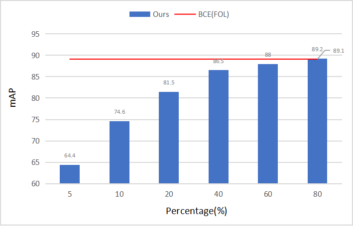
Figure 3: The performance of our approach in POL settings of Pascal VOC. The x-axis represents the percentage of observed labels used in our experiments. For instance, 5 stands for POL_005. The y-axis represents the mAP scores. The score of BCE under FOL setting is shown in red for comparison. Notice that in POL_08, our approach eventually exceeds the performance of BCE with full labels.

V-E Analysis

TABLE IV: The mAP results in PPL settings on COCO, Pascal VOC, and NUSWIDE datasets. PPL_04, PPL_06, and PPL_08 represent randomly retaining 40%, 60% and 80% of positive labels for each instance, respectively, and discarding all negative labels. SPL is equivalent to PPL_single, which is an extreme variation of PPL. In each column we bold the best performing method and underline the second-best except BCE and BCE-LS that is performed under FOL setting.

	COCO				Pascal VOC				NUSWIDE
	SPL	PPL_04	PPL_06	PPL_08	SPL	PPL_04	PPL_06	PPL_08	SPL	PPL_04	PPL_06	PPL_08
BCE (FOL)	75.8				88.9				52.6
BCE-LS (FOL)	76.8				90.0				53.5
AN [54]	63.9	66.4	67.0	69.2	84.7	86.8	87.3	88.0	40.0	45.1	48.3	50.3
WAN [44]	64.8	69.1	70.8	71.2	85.9	87.5	87.9	88.3	43.7	46.9	48.5	50.6
ROLE [4]	65.9	73.1	75.4	77.1	87.0	88.9	90.0	90.3	43.2	48.0	50.4	52.0
Ours	67.8	74.4	75.9	77.8	86.6	88.9	90.8	91.1	46.0	49.6	51.9	53.3

POL. Alleviating the imbalance between positives and negatives is one highlight of our approach. In POL, the impact of the imbalance may be exacerbated since the observable labels are randomly selected. There is equal chance for positive and negative labels to be selected, which means that it is even possible that an instance has multiple positive labels, while another one has no positive labels. This is the reason why most related methods are incompatible with this setting. We opt to use the modified version of AN, WAN, ROLE, Focal and ASL as baseline methods for comparison, and the detailed modification process is described in Sec. V-C.

We conduct experiments on Pascal VOC in POL_02, POL_04, POL_06, and POL_08 settings. The experimental results are shown in Table III. As excepted, since AN does not take imbalance into consideration, it performs the worst among all other methods in our experiments. Moreover, ROLE, which won the second place in PPL setting in our experiments, can not cope with POL setting well. Relying on the ingenious design of the loss function, our method has a significant improvements compared with other baseline-methods. In particular, we notice that the fewer labels are available, the greater the performance of our approach can be over other baselines. Obviously, the experimental results show that our approach can effectively deal with POL settings, which is the most common settings in real world.

To further quantify the impact of the missing ratio of labels on the classification performance, we run our approach in POL_005, POL_01, and the results are summarized in Fig. 3. The performance of our algorithm improves as the number of observed labels increases. Note that in POL_06, we use only 60% of labels and the achieved score is only 1.1% lower than the strong baseline. In POL_08, the performance even exceeds the strong baseline with only 80% of labels. Considering that the cost of annotation is expensive, we can find a balance between 60% and 80% of labels to trade off accuracy of the classifier and the annotation cost.

PPL & SPL. In order to demonstrate the effectiveness of our approach in PPL settings, we consider different labeling settings (PPL_04, PPL_06, PPL_08 and SPL) on three datasets. For fair comparison, we directly execute the official code of AN, WAN and ROLE without any modification as baseline-methods. Meantime, we perform BCE and BCE-LS on these three fully-labeled datasets, i.e., under FOL setting, which are used as strong baselines for our approach. Table IV summarizes the experimental results. For COCO dataset and NUS-WIDE dataset, our algorithm achieves the highest score in all settings. For Pascal VOC, our approach achieves the best mAP score in PPL_04, PPL_06 and PPL_08 settings and the second highest, but comparable, score in SPL setting. These results fully demonstrate that our approach can be effectively applied to PPL settings.

Compared with the strong baselines under FOL setting, the results show that for COCO, our approach can achieve comparable performance to BCE and BCE-LS in PPL_06 and PPL_08, respectively. For Pascal VOC, the results by our approach in PPL_06 and PPL_08 are even able to outperform these two FOL baselines. It is surprising to find that our approach in PPL_04 can even achieve a score comparable to strong baselines, which means we save 26.7% of the cost in labeling positives and 100% cost in labeling negatives, according to the statistics of the labels used in our experiments. As for NUS-WIDE, our method also can reach the strong baselines ,even outperforms BCE(FOL) in PPL_08 setting. However, the other baseline-methods are not able to exceed the strong baselines.

V-F Ablation study

We present an ablation study to measure the contributions of different components in our approach. We run experiments on Pascal VOC in PPL_06 and POL_06. The results are shown in Table V.

TABLE V: The mAP results in ablation study under PPL_06 and POL_06 settings on Pascal VOC.

	PPL_06	POL_06
Ours Approach	90.8	88.0
Without Update	90.1	86.6
Without Disturbances	88.2	86.0
Without Imbalance Design	91.1	76.9
Without Weighted Loss	90.9	79.4

For PPL_06 setting, both our proposed running-average updating method and the introduction of disturbances improve the performance of the approach. However, the novel loss function, including imbalance and weighted design, reduces the performance, because these two factors are designed for more general settings, not specifically for PPL. This can be found in POL_06 setting, where the effectiveness of our design is demonstrated: the imbalance and dynamically weighted design can significantly enhance the performance of the classifier. The former improves the result by more than 11.1%, and the latter improves by 8.6%. In contrast, the new updating method and disturbance have relatively limited, but still positive, improvements in POL setting (more than 1% increase).

VI Conclusion

This paper explores the problem of multi-label classification with missing labels. We propose a novel pseudo-label-based approach to cope with missing-label problem without increasing the complexity of the existing classification networks. By leveraging prior knowledge of the dataset, our approach relaxes the assumption that each instance in the training set must has at least one positive label, which is often required in existing approaches. We demonstrate the effectiveness of our approach by performing extensive experiments on three large-scale datasets. It is shown that our method can effectively reduce the annotation cost without significant degradation in classification performance. We also evaluate the impact of the missing ratio of the labels on the classifier’s performance, which can be used as a guideline to achieve the balance between performance and labeling costs.

References

- [1] G. Tsoumakas and I. Katakis, “Multi-label classification: An overview,” International Journal of Data Warehousing and Mining (IJDWM), vol. 3, no. 3, pp. 1–13, 2007.
- [2] T. Durand, N. Mehrasa, and G. Mori, “Learning a deep convnet for multi-label classification with partial labels,” in Proceedings of the IEEE/CVF Conference on Computer Vision and Pattern Recognition, 2019, pp. 647–657.
- [3] T. Hastie, R. Tibshirani, and J. Friedman, “Overview of supervised learning,” in The elements of statistical learning. Springer, 2009, pp. 9–41.
- [4] E. Cole, O. Mac Aodha, T. Lorieul, P. Perona, D. Morris, and N. Jojic, “Multi-label learning from single positive labels,” in Proceedings of the IEEE/CVF Conference on Computer Vision and Pattern Recognition, 2021, pp. 933–942.
- [5] Y. Zhang, Y. Cheng, X. Huang, F. Wen, R. Feng, Y. Li, and Y. Guo, “Simple and robust loss design for multi-label learning with missing labels,” arXiv preprint arXiv:2112.07368, 2021.
- [6] M. A. Hedderich and D. Klakow, “Training a neural network in a low-resource setting on automatically annotated noisy data,” arXiv preprint arXiv:1807.00745, 2018.
- [7] D. Mahajan, R. Girshick, V. Ramanathan, K. He, M. Paluri, Y. Li, A. Bharambe, and L. Van Der Maaten, “Exploring the limits of weakly supervised pretraining,” in Proceedings of the European conference on computer vision (ECCV), 2018, pp. 181–196.
- [8] C. Sun, A. Shrivastava, S. Singh, and A. Gupta, “Revisiting unreasonable effectiveness of data in deep learning era,” in Proceedings of the IEEE international conference on computer vision, 2017, pp. 843–852.
- [9] W. A. Smith and R. B. Randall, “Rolling element bearing diagnostics using the case western reserve university data: A benchmark study,” Mechanical systems and signal processing, vol. 64, pp. 100–131, 2015.
- [10] M. Bin Hasan, “Model-free drive system current monitoring: faults detection and diagnosis through statistical features extraction and support vector machines classification. current based condition monitoring of electromechanical systems,” Ph.D. dissertation, Thesis (Ph. D.). School of Engineering Design and Technology, University of …, 2012.
- [11] D. Lee, V. Siu, R. Cruz, and C. Yetman, “Convolutional neural net and bearing fault analysis,” in Proceedings of the International Conference on Data Science (ICDATA). The Steering Committee of The World Congress in Computer Science, Computer …, 2016, p. 194.
- [12] B. Wu, S. Lyu, and B. Ghanem, “Ml-mg: Multi-label learning with missing labels using a mixed graph,” in Proceedings of the IEEE international conference on computer vision, 2015, pp. 4157–4165.
- [13] M.-L. Zhang, Y.-K. Li, X.-Y. Liu, and X. Geng, “Binary relevance for multi-label learning: an overview,” Frontiers of Computer Science, vol. 12, no. 2, pp. 191–202, 2018.
- [14] R. Cabral, F. Torre, J. P. Costeira, and A. Bernardino, “Matrix completion for multi-label image classification,” Advances in neural information processing systems, vol. 24, 2011.
- [15] M. Xu, R. Jin, and Z.-H. Zhou, “Speedup matrix completion with side information: Application to multi-label learning,” Advances in neural information processing systems, vol. 26, 2013.
- [16] H. Yang, J. T. Zhou, and J. Cai, “Improving multi-label learning with missing labels by structured semantic correlations,” in European conference on computer vision. Springer, 2016, pp. 835–851.
- [17] M. Chen, A. Zheng, and K. Weinberger, “Fast image tagging,” in International conference on machine learning. PMLR, 2013, pp. 1274–1282.
- [18] S. Kornblith, J. Shlens, and Q. V. Le, “Do better imagenet models transfer better?” in Proceedings of the IEEE/CVF conference on computer vision and pattern recognition, 2019, pp. 2661–2671.
- [19] X. Li and B. Liu, “Learning to classify texts using positive and unlabeled data,” in IJCAI, vol. 3, no. 2003. Citeseer, 2003, pp. 587–592.
- [20] B. Liu, W. S. Lee, P. S. Yu, and X. Li, “Partially supervised classification of text documents,” in ICML, vol. 2, no. 485. Sydney, NSW, 2002, pp. 387–394.
- [21] X. Li, B. Liu, and S.-K. Ng, “Learning to identify unexpected instances in the test set.” in IJCAI, vol. 7, 2007, pp. 2802–2807.
- [22] H. Yu, J. Han, and K. C.-C. Chang, “Pebl: positive example based learning for web page classification using svm,” in Proceedings of the eighth ACM SIGKDD international conference on Knowledge discovery and data mining, 2002, pp. 239–248.
- [23] S. Sellamanickam, P. Garg, and S. K. Selvaraj, “A pairwise ranking based approach to learning with positive and unlabeled examples,” in Proceedings of the 20th ACM international conference on Information and knowledge management, 2011, pp. 663–672.
- [24] M. Claesen, F. De Smet, J. A. Suykens, and B. De Moor, “A robust ensemble approach to learn from positive and unlabeled data using svm base models,” Neurocomputing, vol. 160, pp. 73–84, 2015.
- [25] L. Jiang, H. Zhang, and Z. Cai, “A novel bayes model: Hidden naive bayes,” IEEE Transactions on knowledge and data engineering, vol. 21, no. 10, pp. 1361–1371, 2008.
- [26] C. Liang, Y. Zhang, P. Shi, and Z. Hu, “Learning very fast decision tree from uncertain data streams with positive and unlabeled samples,” Information Sciences, vol. 213, pp. 50–67, 2012.
- [27] J. Bekker and J. Davis, “Learning from positive and unlabeled data: A survey,” Machine Learning, vol. 109, no. 4, pp. 719–760, 2020.
- [28] D.-H. Lee et al., “Pseudo-label: The simple and efficient semi-supervised learning method for deep neural networks,” in Workshop on challenges in representation learning, ICML, vol. 3, no. 2, 2013, p. 896.
- [29] W. Shi, Y. Gong, C. Ding, Z. M. Tao, and N. Zheng, “Transductive semi-supervised deep learning using min-max features,” in Proceedings of the European Conference on Computer Vision (ECCV), 2018, pp. 299–315.
- [30] M. N. Rizve, K. Duarte, Y. S. Rawat, and M. Shah, “In defense of pseudo-labeling: An uncertainty-aware pseudo-label selection framework for semi-supervised learning,” arXiv preprint arXiv:2101.06329, 2021.
- [31] A. Iscen, G. Tolias, Y. Avrithis, and O. Chum, “Label propagation for deep semi-supervised learning,” in Proceedings of the IEEE/CVF Conference on Computer Vision and Pattern Recognition, 2019, pp. 5070–5079.
- [32] G.-H. Wang and J. Wu, “Repetitive reprediction deep decipher for semi-supervised learning,” in Proceedings of the AAAI Conference on Artificial Intelligence, vol. 34, no. 04, 2020, pp. 6170–6177.
- [33] D. Berthelot, N. Carlini, I. Goodfellow, N. Papernot, A. Oliver, and C. A. Raffel, “Mixmatch: A holistic approach to semi-supervised learning,” Advances in Neural Information Processing Systems, vol. 32, 2019.
- [34] D. Berthelot, N. Carlini, E. D. Cubuk, A. Kurakin, K. Sohn, H. Zhang, and C. Raffel, “Remixmatch: Semi-supervised learning with distribution alignment and augmentation anchoring,” arXiv preprint arXiv:1911.09785, 2019.
- [35] K. Sohn, D. Berthelot, N. Carlini, Z. Zhang, H. Zhang, C. A. Raffel, E. D. Cubuk, A. Kurakin, and C.-L. Li, “Fixmatch: Simplifying semi-supervised learning with consistency and confidence,” Advances in Neural Information Processing Systems, vol. 33, pp. 596–608, 2020.
- [36] Q. Xie, Z. Dai, E. Hovy, T. Luong, and Q. Le, “Unsupervised data augmentation for consistency training,” Advances in Neural Information Processing Systems, vol. 33, pp. 6256–6268, 2020.
- [37] H. Zhang, Z. Zhang, A. Odena, and H. Lee, “Consistency regularization for generative adversarial networks,” arXiv preprint arXiv:1910.12027, 2019.
- [38] T. Ridnik, E. Ben-Baruch, N. Zamir, A. Noy, I. Friedman, M. Protter, and L. Zelnik-Manor, “Asymmetric loss for multi-label classification,” in Proceedings of the IEEE/CVF International Conference on Computer Vision, 2021, pp. 82–91.
- [39] F. Scarselli, M. Gori, A. C. Tsoi, M. Hagenbuchner, and G. Monfardini, “The graph neural network model,” IEEE transactions on neural networks, vol. 20, no. 1, pp. 61–80, 2008.
- [40] J. Nam, J. Kim, E. Loza Mencía, I. Gurevych, and J. Fürnkranz, “Large-scale multi-label text classification—revisiting neural networks,” in Joint european conference on machine learning and knowledge discovery in databases. Springer, 2014, pp. 437–452.
- [41] J. Wang, Y. Yang, J. Mao, Z. Huang, C. Huang, and W. Xu, “Cnn-rnn: A unified framework for multi-label image classification,” in Proceedings of the IEEE conference on computer vision and pattern recognition, 2016, pp. 2285–2294.
- [42] M. S. Sorower, “A literature survey on algorithms for multi-label learning,” Oregon State University, Corvallis, vol. 18, pp. 1–25, 2010.
- [43] Y.-Y. Sun, Y. Zhang, and Z.-H. Zhou, “Multi-label learning with weak label,” in Twenty-fourth AAAI conference on artificial intelligence, 2010.
- [44] O. Mac Aodha, E. Cole, and P. Perona, “Presence-only geographical priors for fine-grained image classification,” in Proceedings of the IEEE/CVF International Conference on Computer Vision, 2019, pp. 9596–9606.
- [45] S. S. Bucak, R. Jin, and A. K. Jain, “Multi-label learning with incomplete class assignments,” in CVPR 2011. IEEE, 2011, pp. 2801–2808.
- [46] A. Joulin, L. v. d. Maaten, A. Jabri, and N. Vasilache, “Learning visual features from large weakly supervised data,” in European Conference on Computer Vision. Springer, 2016, pp. 67–84.
- [47] Y. Wang, X. Ma, Z. Chen, Y. Luo, J. Yi, and J. Bailey, “Symmetric cross entropy for robust learning with noisy labels,” in Proceedings of the IEEE/CVF International Conference on Computer Vision, 2019, pp. 322–330.
- [48] T.-Y. Lin, P. Goyal, R. Girshick, K. He, and P. Dollár, “Focal loss for dense object detection,” in Proceedings of the IEEE international conference on computer vision, 2017, pp. 2980–2988.
- [49] P. Morerio, J. Cavazza, R. Volpi, R. Vidal, and V. Murino, “Curriculum dropout,” in IEEE International Conference on Computer Vision (ICCV), 2017, pp. 3544–3552.
- [50] T.-Y. Lin, M. Maire, S. Belongie, J. Hays, P. Perona, D. Ramanan, P. Dollár, and C. L. Zitnick, “Microsoft coco: Common objects in context,” in European conference on computer vision. Springer, 2014, pp. 740–755.
- [51] T.-S. Chua, J. Tang, R. Hong, H. Li, Z. Luo, and Y. Zheng, “Nus-wide: a real-world web image database from national university of singapore,” in Proceedings of the ACM international conference on image and video retrieval, 2009, pp. 1–9.
- [52] M. Everingham, S. Eslami, L. Van Gool, C. K. Williams, J. Winn, and A. Zisserman, “The pascal visual object classes challenge: A retrospective,” International journal of computer vision, vol. 111, no. 1, pp. 98–136, 2015.
- [53] C. Szegedy, V. Vanhoucke, S. Ioffe, J. Shlens, and Z. Wojna, “Rethinking the inception architecture for computer vision,” in Proceedings of the IEEE conference on computer vision and pattern recognition, 2016, pp. 2818–2826.
- [54] K. Kundu and J. Tighe, “Exploiting weakly supervised visual patterns to learn from partial annotations,” Advances in Neural Information Processing Systems, vol. 33, pp. 561–572, 2020.
- [55] S. Xie, R. Girshick, P. Dollár, Z. Tu, and K. He, “Aggregated residual transformations for deep neural networks,” in Proceedings of the IEEE conference on computer vision and pattern recognition, 2017, pp. 1492–1500.
- [56] J. Deng, W. Dong, R. Socher, L.-J. Li, K. Li, and F.-F. Li, “Imagenet: A large-scale hierarchical image database,” in 2009 IEEE conference on computer vision and pattern recognition. Ieee, 2009, pp. 248–255.