Supplemental Material: Effective Landé factors of electrons and holes in lead chalcogenide nanocrystals

Abstract

This supporting information contains the: Explicit form of matrices entering Eq.(1). Details of TB calculations. Comparison of results obtained for NCs of different shape. Illustration of accuracy of effective $g$-factor extraction. Details of calculations in isotropic and anisotropic k$\cdot$p model. Discussion of off-diagonal terms in effective magnetic field Hamiltonian. Explicit form of the matrices transforming the basis functions of independent valleys to the basis of irreducible representations of the group $T_{d}$. Some mathematical expressions used in k$\cdot$p calculations.

S1 Matrices entering Eq. (1)

The matrices $J_{\gamma}$ ($\gamma=x,y,z$) are given by

$$J_{x}=\begin{pmatrix}0&\frac{\sqrt{3}}{2}&0&0\\ \frac{\sqrt{3}}{2}&0&1&0\\ 0&1&0&\frac{\sqrt{3}}{2}\\ 0&0&\frac{\sqrt{3}}{2}&0\end{pmatrix}\,,$$ (S1a)

$$J_{y}=\begin{pmatrix}0&-\frac{{\rm i}\sqrt{3}}{2}&0&0\\ \frac{{\rm i}\sqrt{3}}{2}&0&-{\rm i}&0\\ 0&{\rm i}&0&-\frac{{\rm i}\sqrt{3}}{2}\\ 0&0&\frac{{\rm i}\sqrt{3}}{2}&0\end{pmatrix}\,,$$ (S1b)

$$J_{z}=\begin{pmatrix}\frac{3}{2}&0&0&0\\ 0&\frac{1}{2}&0&0\\ 0&0&-\frac{1}{2}&0\\ 0&0&0&-\frac{3}{2}\end{pmatrix}\,.$$ (S1c)

They are written in the basis $(\left|j\right\rangle,\left|j-1\right\rangle,\ldots,\left|-j\right\rangle)$ [1].

S2 Tight-binding calculations

We follow the procedure described in Refs. 2, 3, 4 and use the extended tight-binding model [5, 6] to compute the energies and wave functions of electron states in the conduction and valence bands for NCs of various shapes and classify them in accordance with irreducible representations of the point group $T_{d}$ [4] (we restrict our consideration to stoichiometric NCs with no inversion center). The effect of the magnetic field is taken into account using the standard procedure of Ref. 7.

From the energy splittings induced by the external magnetic field we extract the constants in the effective Hamiltonain (1). NCs of cubic, octaherdal, and cuboctahedral shapes and various sizes are used in the calculations (see Refs. 8 and 4 for details). The effective NC diameter is calculated as a diameter of the sphere with the same volume as the NC. NCs with quasi-spherical shapes [6] are obtained as a set of atoms of the bulk material located within a sphere with the diameter $D$ and the center lying halfway between a cation and an anion on a line parallel to the $\langle 111\rangle$ direction.

S3 Nanocrystals of various shapes

In the main text we show only the effective $g$-factors calculated for the quasi-spherical NCs with $T_{d}$ point group symmetry. They are obtained as a set of atoms of the bulk material located within a sphere with the diameter $D$ and the center lying halfway between a cation and an anion on a line parallel to the $\langle 111\rangle$ direction.[6] In figure 1 we give the intra-valley $g$-factors extracted from the tight-binding calculations for NCs of various shapes: quasi-spherical, octahedral, cubic, and cuboctahedron.

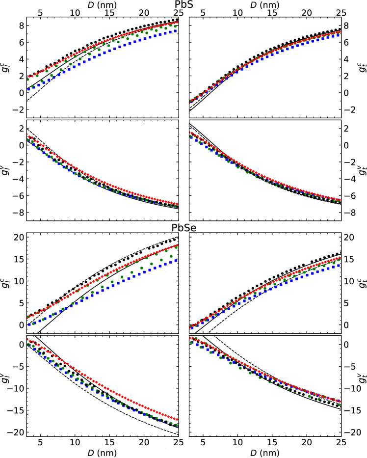
Figure 1: Shape dependence of the effective valley $g$-factors in PbS (top four panels) and PbSe (lower four panels) NCs. Shape and color of the symbols represent the shapes of the NCs: cubic (blue), cuboctahedral (green), octahedral (red), and spherical (black). Solid (dashed) lines show outcomes of the anisotropic (isotropic) k$\cdot$p model.

S4 Accuracy of $g$-factor determination

Since the numbers of independent constants in equations (1) and (3) are different (four versus two), determination of the effective valley $g$-factors introduces an error. In order to estimate it, in figure 2 we show the deviation of $g_{6}^{\eta}$ and $g_{7}^{\eta}$, calculated using the tight-binding method, from their counterparts obtained with the help of $g^{\eta}_{l}$ and $g^{\eta}_{t}$.

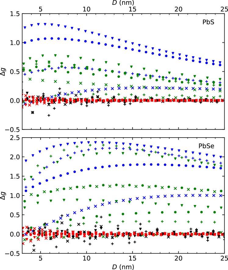
Figure 2: Difference between the values $g_{6}$ ($\bullet$, +), $g_{7}$ ($\blacktriangledown$, $\times$) extracted from the tight-binding calculations and the values of these $g$-factors calculated after phenomenological Eqs. (5) in conduction band ($\bullet$,$\blacktriangledown$) and valence band ($+$,$\times$). Color of the symbols represents the shapes of the NCs: cubic (blue), cuboctahedral (green), octahedral (red) and spherical (black).

S5 k$\cdot$p model

In the k$\cdot$p calculations, we use the single-valley model of Ref. 9. Energies of the electron states with a given value of $F$, confined in a spherical NC, are found from the dispersion equations

$$i^{(1)}_{F-\frac{p}{2}}(k_{-}R)j_{F+\frac{p}{2}}(k_{+}R)\rho_{-}\\ -p\,i^{(1)}_{F+\frac{p}{2}}(k_{-}R)j_{F-\frac{p}{2}}(k_{+}R)\rho_{+}=0\,,$$ (S2)

where $p=\pm 1$ is an additional quantum number, related to the parity,

$$\Lambda(E) =\frac{E(\alpha_{v}-\alpha_{c})-\frac{\hbar^{2}P^{2}}{m_{0}^{2}}-\frac{(\alpha_{v}+\alpha_{c})E_{g}}{2}}{2\alpha_{c}\alpha_{v}}\,,$$ (S3a)

$$\Sigma(E) =\sqrt{\Lambda^{2}(E)+\frac{E^{2}-(E_{g}/2)^{2}}{\alpha_{c}\alpha_{v}}}\,,$$ (S3b)

$$k_{\pm}(E) =\sqrt{\Sigma(E)\pm\Lambda(E)}\,,$$ (S3c)

$$\rho_{\pm}(E) =\frac{E_{g}/2\pm\alpha_{c}k_{\pm}^{2}(E)-E}{(\hbar P/m_{0})k_{\pm}(E)}\,.$$ (S3d)

For each $p=\pm 1$ there are positive (conduction band) and negative (valence band) roots $E_{n}$ of the equation (S2). We enumerate energy levels in each band separately starting from $n=0$.

The explicit forms of the normalized radial functions in Eq. (8) are

$$\begin{split}f_{\ell p}(r)=&A\left[j_{\ell}(k_{+}r)-\frac{j_{\ell}(k_{+}R)}{i^{(1)}_{\ell}(k_{-}R)}i^{(1)}_{\ell}(k_{-}r)\right]\,,\\ g_{\ell p}(r)=&A\left[\rho_{+}j_{\ell}(k_{+}r)-p\rho_{-}\frac{j_{\ell-p}(k_{+}R)}{i^{(1)}_{\ell-p}(k_{-}R)}i^{(1)}_{\ell}(k_{-}r)\right]\,.\end{split}$$ (S4)

Here $j_{\ell}$ and $i_{\ell}^{(1)}$ are, respectively, the spherical Bessel and modified spherical Bessel functions of the first kind. The normalization constant $A$ is determined from the condition

$$\int\limits_{0}^{R}\left[f_{\ell p}^{2}(r)+g_{\ell p}^{2}(r)\right]r^{2}\mathrm{d}r=1\,.$$ (S5)

Since Eq. (8) is written in the basis of conduction and valence band Bloch functions which are, respectively, odd and even, the partiy of the resulting wave function $\left|F,p,n,F_{z}\right\rangle$ is $\pi=(-1)^{F+\frac{p}{2}}$.

S6 Anisotropic effective mass model

The effective Hamiltonian of the anisotropic model takes the form 9

$$H_{\text{aniso}}=\begin{pmatrix}\left(\frac{E_{g}}{2}-\alpha_{c}^{t}\frac{\partial^{2}}{\partial x^{2}}-\alpha_{c}^{t}\frac{\partial^{2}}{\partial y^{2}}-\alpha_{c}^{l}\frac{\partial^{2}}{\partial z^{2}}\right)&-\frac{i\hbar}{m_{0}}\left(P_{t}\sigma_{x}\frac{\partial}{\partial x}+P_{t}\sigma_{y}\frac{\partial}{\partial y}+P_{l}\sigma_{z}\frac{\partial}{\partial z}\right)\\ -\frac{i\hbar}{m_{0}}\left(P_{t}\sigma_{x}\frac{\partial}{\partial x}+P_{t}\sigma_{y}\frac{\partial}{\partial y}+P_{l}\sigma_{z}\frac{\partial}{\partial z}\right)&-\left(\frac{E_{g}}{2}-\alpha_{v}^{t}\frac{\partial^{2}}{\partial x^{2}}-\alpha_{v}^{t}\frac{\partial^{2}}{\partial y^{2}}-\alpha_{v}^{l}\frac{\partial^{2}}{\partial z^{2}}\right)\end{pmatrix}\,,$$ (S6)

where $P_{t}$ and $P_{l}$ are transverse and longitudinal interband momentum matrix elements and $\alpha_{c(v)}^{t(l)}$ describe contributions to the energy dispersion from the remote bands; $x$, $y$, $z$ are the local coordinates of the valley. The Schrödinger equation with this Hamiltonian can be solved numerically in the basis of the solutions of the isotropic model (8).

An external magnetic field can be taken into account using analogs of equations (9), (10). The resulting Hamiltonian takes the form $H_{\text{aniso}}+H_{\text{aniso}}({\bf B})$, where

$$H_{\text{aniso}}({\bf B})=H^{\prime}_{\text{iso}}({\bf B})+\delta H_{P}({\bf B})+\delta H_{\alpha}({\bf B})\,.$$ (S7)

Here $H^{\prime}_{\text{iso}}({\bf B})$ has the same form as Eq. (10), with the electron and hole $g$-factors renormalized in accordance with[10]

$$\begin{split}g_{t,\text{bulk}}^{c}=g^{c}_{0t}+\frac{4P_{t}P_{l}}{E_{g}m_{0}}\,,\qquad&g_{l,\text{bulk}}^{c}=g^{c}_{0l}+\frac{4P_{t}^{2}}{E_{g}m_{0}}\,,\\ g_{t,\text{bulk}}^{v}=g^{v}_{0t}-\frac{4P_{t}P_{l}}{E_{g}m_{0}}\,,\qquad&g_{l,\text{bulk}}^{v}=g^{v}_{0l}-\frac{4P_{t}^{2}}{E_{g}m_{0}}\,.\end{split}$$ (S8)

The remaining two terms in the right-hand side of equation (S7) can be written as follows: $\delta H_{P}({\bf B})=\delta H_{P,l}({\bf B})+\delta H_{P,t}({\bf B})$, where

$$\delta H_{P,l}({\bf B})=\mu_{B}\frac{P_{l}-P}{\hbar}\sigma_{z}\left(B_{x}y-B_{y}x\right)\begin{pmatrix}0&1\\ 1&0\end{pmatrix}$$ (S9a)

$$\delta H_{P,t}({\bf B})=\mu_{B}\frac{P_{t}-P}{\hbar}\big{[}z\left(\sigma_{x}B_{y}-\sigma_{y}B_{x}\right)+B_{z}\left(x\sigma_{y}-y\sigma_{x}\right)\big{]}\begin{pmatrix}0&1\\ 1&0\end{pmatrix}\,,$$ (S9b)

and $\delta H_{\alpha}({\bf B})=\delta H_{\alpha,l}({\bf B})+\delta H_{\alpha,t}({\bf B})$, where

$$\delta H_{\alpha,l}({\bf B})=-{\rm i}\mu_{B}(B_{x}y-B_{y}x)\nabla_{z}\\ \times\frac{2m_{0}}{\hbar^{2}}\begin{pmatrix}(\alpha_{c}^{l}-\alpha_{c})&0\\ 0&-(\alpha_{v}^{l}-\alpha_{v})\end{pmatrix}\,,$$ (S10a)

$$\delta H_{\alpha,t}({\bf B})=-{\rm i}\mu_{B}\left[z(B_{y}\nabla_{x}-B_{x}\nabla_{y})+{\rm i}B_{z}L_{z}\right]\\ \frac{2m_{0}}{\hbar^{2}}\begin{pmatrix}(\alpha_{c}^{t}-\alpha_{c})&0\\ 0&-(\alpha_{v}^{t}-\alpha_{v})\end{pmatrix}\,.$$ (S10b)

Using the Wigner-Eckart theorem, each correction term, Eqs. (S9), (S10), can be decomposed into a one-dimensional integral containing the radial functions (S4) and an angular part. Both these parts are computed numerically. In practical calculations, it is enough to restrict the basis of unperturbed states by few confined states of the isotropic model with total angular momentum $F\leq 5/2$.

	PbS	PbSe
$E_{g}$ (eV)	$0.29397$	$0.21288$
$\alpha_{v}^{t}\,m_{0}/\hbar^{2}$	$3.71261$	$3.61848$
$\alpha_{v}^{l}\,m_{0}/\hbar^{2}$	$0.48082$	$0.78444$
$\alpha_{c}^{t}\,m_{0}/\hbar^{2}$	$3.35927$	$3.00629$
$\alpha_{c}^{l}\,m_{0}/\hbar^{2}$	$0.69673$	$0.94606$
$2P_{t}^{2}/m_{0}$ (eV)	$1.67733$	$3.96341$
$2P_{l}^{2}/m_{0}$ (eV)	$2.42323$	$2.73803$
$g_{t,\text{bulk}}^{v}$	$-9.62387$	$-24.19664$
$g_{l,\text{bulk}}^{v}$	$-9.99538$	$-31.45314$
$g_{t,\text{bulk}}^{c}$	$10.13564$	$25.99249$
$g_{l,\text{bulk}}^{c}$	$11.05293$	$31.26533$

Table 1: The parameters of the anisotropic k$\cdot$p model, $m_{0}$ is the free electron mass.

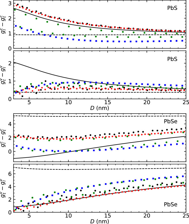
Figure 3: Differences in the longitudinal $g^{\eta}_{l}$ and transverse $g^{\eta}_{t}$ $g$-factors in the conduction ($\eta=c$) and valence ($\eta=v$) bands of PbX quantum dots. The outcomes of the anisotropic (isotropic) k$\cdot$p models are shown by solid (dashed) lines. By symbols are shown the corresponding values calculated in the tight-binding method for NCs of cubic (blue), cuboctahedral (green), octahedral (red), and quasi-spherical (black) shapes.

While both isotropic and anisotropic k$\cdot$p models provide a good agreement with the tight-binding calculations of the $g$-factor, only anisotropic one can account for the difference in longitudinal and transverse $g$-factors introduced by their renormalization. This is illustrated in Fig. 3 where the differences between longitudinal and transverse $g$-factors in the conduction and valence bands, $(g^{c}_{l}-g^{c}_{t})$ and $(g^{v}_{t}-g^{v}_{l})$, are shown. One can see that, in the isotropic model, the difference is almost constant.

S7 The off-diagoinal terms

The symmetry-allowed off-diagonal corrections to the Hamiltonian (1) are

$$\delta{H}_{1}^{\eta}({\bf B})=\mu_{B}{\bf B}\begin{pmatrix}0&0&g_{68}{\bf J}_{68}\\ 0&0&g_{78}{\bf J}_{78}\\ g_{68}{\bf J}_{68}^{{\dagger}}&g_{78}{\bf J}_{78}^{{\dagger}}&0\\ \end{pmatrix}\,.$$ (S11)

This form of the Hamiltonian follows from the fact that the $\Gamma_{6}\otimes\Gamma_{8}$ and $\Gamma_{7}\otimes\Gamma_{8}$ reducible representations contain the irreducible $\Gamma_{4}$ (pseudovector) representation of the group $T_{d}$. Here ${\bf J}_{68}$ are the matrices transforming under the irreducible representation $\Gamma_{4}$ of the point group $T_{d}$ and asymmetric with respect to time inversion, written in the basis $\Gamma_{6}\otimes\Gamma_{8}$. Their explicit form is

$$[J_{68}]_{x} =\begin{pmatrix}-\frac{\sqrt{3}}{2}&0&\frac{1}{2}&0\\ 0&-\frac{1}{2}&0&\frac{\sqrt{3}}{2}\end{pmatrix}\,,$$ (S12a)

$$[J_{68}]_{y} =-{\rm i}\begin{pmatrix}\frac{\sqrt{3}}{2}&0&\frac{1}{2}&0\\ 0&\frac{1}{2}&0&\frac{\sqrt{3}}{2}\end{pmatrix}\,,$$ (S12b)

$$[J_{68}]_{z} =\begin{pmatrix}0&1&0&0\\ 0&0&1&0\end{pmatrix}\,,$$ (S12c)

where rows correspond to the basis functions of $\Gamma_{6}$ and columns correspond to the basis functions of $\Gamma_{8}$. ${\bf J}_{78}$ are analogous matrices in the basis $\Gamma_{7}\otimes\Gamma_{8}$:

$$[J_{78}]_{x} =\begin{pmatrix}\frac{1}{2}&0&\frac{\sqrt{3}}{2}&0\\ 0&-\frac{\sqrt{3}}{2}&0&-\frac{1}{2}\end{pmatrix}\,,$$ (S13a)

$$[J_{78}]_{y} ={\rm i}\begin{pmatrix}-\frac{1}{2}&0&\frac{\sqrt{3}}{2}&0\\ 0&\frac{\sqrt{3}}{2}&0&-\frac{1}{2}\end{pmatrix}\,,$$ (S13b)

$$[J_{78}]_{z} =\begin{pmatrix}0&0&0&1\\ 1&0&0&0\end{pmatrix}\,.$$ (S13c)

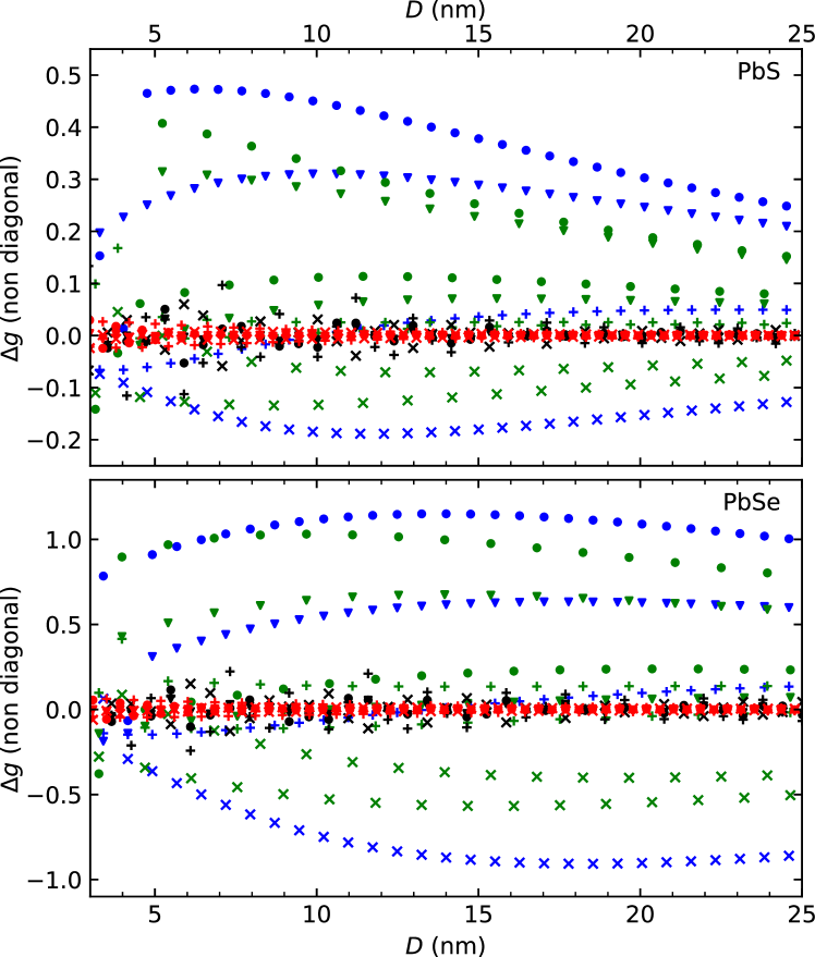
Figure 4: Deviations of the values $g_{68}$ ($\bullet$, +) and $g_{78}$ ($\blacktriangledown$, $\times$) extracted from tight-binding calculations from phenomenological equations (S14) in conduction band ($\bullet$,$\blacktriangledown$) and valence band ($+$,$\times$). Color of the symbols represents the shapes of the quantum dots: cubic (blue), cuboctahedral (green), octahedral (red) and spherical (black).

Comparison with equation (3) yields the following relation of $g_{68}$ and $g_{78}$ to the $g$-factors in $L$ valleys:

$$g_{68}^{c}=\frac{g_{l}^{c}+g_{t}^{c}}{3\sqrt{2}}\,,\quad g_{78}^{c}=\frac{g_{l}^{c}-g_{t}^{c}}{3\sqrt{2}}\,,$$ (S14a)

$$g_{68}^{v}=\frac{g_{l}^{c}-g_{t}^{c}}{3\sqrt{2}}\,,\quad g_{78}^{v}=-\frac{g_{l}^{c}+g_{t}^{c}}{3\sqrt{2}}\,.$$ (S14b)

The difference between the values $g_{68}$ and $g_{78}$ extracted from the tight-binding calculations and calculated from the phenomenological equations (S14) are shown in Figure 4. It is clear that this difference qualitatively follows the same trend as the values of the valley splittings, see Ref. 4: they are relatively large in cubic (blue), smaller in cuboctahedral (green) and even smaller in octahedral (red) and quasi-spherical (black) NCs. In all cases, the deviations vanish with the increase of NC diameter.

S8 Transformation matrices

In this Section we define transformation matrices between the basis of electronic states in independent valleys with valley-specific coordinate axes and the basis of combinations of valley states transforming according to irreducible representations $\Gamma_{6}$, $\Gamma_{7}$, and $\Gamma_{8}$ ($\Gamma^{\pm}_{6}$, $\Gamma^{\pm}_{7}$, and $\Gamma^{\pm}_{8}$) of the point group $T_{d}$ ($O_{h}$). The latter basis is defined using the laboratory reference frame with the coordinate axes $x,y,$ and $z$ along the $[100]$, $[010]$, and $[001]$ directions, respectively (see Figure 5).

We begin with the $L_{0}$ valley. In this valley the ground electron (hole) states form the basis of the $\Gamma_{4}^{\mp}$ irreducible representation of the $D_{3d}$ group of the wave vector ${\bf k}_{0}$. Within the isotropic k$\cdot$p model (see Methods and Refs. 9, 4), electron (hole) states are associated with pseudo-spinors (spinors) transforming under $D_{1/2}^{-}$ ($D_{1/2}^{+}$) representations of the three-dimensional orthogonal group $O(3)$. In the other three valleys $L_{\mu}$ ($\mu=1,2,3$) we define the bases via $C_{2}$ rotations of the basis in the $L_{0}$ valley (see Figure 5 and Ref. 2) as follows:

$$L_{0}\to L_{1}\;\mbox{via}\;C_{2}^{[001]}\,,\;\;L_{0}\to L_{2}\;\mbox{via}\;C_{2}^{[100]}\,,\;\;L_{0}\to L_{3}\;\mbox{via}\;C_{2}^{[010]}\,.$$ (S15)

The joint basis, combining all the four valley bases, represents the spin-valley basis of the star of the wave vector ${\bf k}_{0}$ in $T_{d}$ (or $O_{h}$) point group.

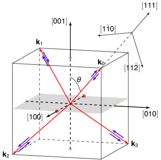
Figure 5: The valley wave vectors ${\bf k}_{\nu}$ (red arrows) serve as directions used to define “spin” (total angular momentum) projections $F_{z}=\pm 1/2$ (blue arrows) in their respective valley coordinate frames. The axes of the laboratory frame are along the $[100]$, $[010]$, and $[001]$ directions (bold black arrows).

With this definition, one may find the matrices which transform the spin-valley basis to the bases of irreducible representations $\Gamma_{6},\Gamma_{7}$, and $\Gamma_{8}$ of the group $T_{d}$. It is convenient to write the transformation matrices $S_{c(v)}$ as products of the three matrices:

$$S_{c(v)}=DV_{s}U_{c(v)}\,.$$ (S16)

Here the first matrix $D$ affects only spin degrees of freedom. It is a block-diagonal matrix which transforms spin states, defined in the coordinate frames of their respective valleys, to the states with certain spin projections along $z\parallel[001]$:

$$D=\operatorname{diag}\left\{D_{0},D_{1},D_{2},D_{3}\right\}\,.$$ (S17)

The blocks are given by

$$D_{0} =\begin{pmatrix}c_{c}e^{-{\rm i}\frac{\pi}{8}}&-{\rm i}s_{c}e^{{\rm i}\frac{\pi}{8}}\\ -{\rm i}s_{c}e^{-{\rm i}\frac{\pi}{8}}&\phantom{-}c_{c}e^{\rm{\rm i}\frac{\pi}{8}}\end{pmatrix}\,,\;\; D_{1} =\begin{pmatrix}\phantom{-}{\rm i}c_{c}e^{-{\rm i}\frac{\pi}{8}}&-s_{c}e^{{\rm i}\frac{\pi}{8}}\\ \phantom{-}s_{c}e^{-{\rm i}\frac{\pi}{8}}&-{\rm i}c_{c}e^{{\rm i}\frac{\pi}{8}}\end{pmatrix}\,,$$ (S18a)

$$D_{2} =\begin{pmatrix}\phantom{-}s_{c}e^{{\rm i}\frac{\pi}{8}}&\phantom{-}{\rm i}c_{c}e^{-{\rm i}\frac{\pi}{8}}\\ \phantom{-}{\rm i}c_{c}e^{{\rm i}\frac{\pi}{8}}&\phantom{-}s_{c}e^{-{\rm i}\frac{\pi}{8}}\end{pmatrix}\,,\;\; \;\;\;\;\;D_{3} =\begin{pmatrix}\phantom{-}{\rm i}s_{c}e^{{\rm i}\frac{\pi}{8}}&c_{c}e^{-{\rm i}\frac{\pi}{8}}\\ -c_{c}e^{{\rm i}\frac{\pi}{8}}&-{\rm i}s_{c}e^{-{\rm i}\frac{\pi}{8}}\end{pmatrix}\,,$$ (S18b)

where $c_{c}=\sqrt{\frac{\sqrt{3}+1}{2\sqrt{3}}}$ and $s_{c}=\sqrt{\frac{\sqrt{3}-1}{2\sqrt{3}}}$. These blocks were obtained assuming the following relation between spinors aligned along $z$ and along the $L_{\mu}$ valley axes

$$g_{0\to\mu}g_{x^{\prime}}g_{z}({\uparrow}_{z})={\uparrow}_{\mu}\,,\;\;\;\;\;g_{0\to\mu}g_{x^{\prime}}g_{z}({\downarrow}_{z})={\downarrow}_{\mu}\,,$$ (S19)

where $g_{0\to\mu}$ is one of the three $C_{2}$ rotations (S15) or the identity transformation (for the $L_{0}$ valley) and the rotation $g_{x^{\prime}}g_{z}$ transforms the crystallographic axes $xyz$ to the coordinate frame of the $L_{0}$ valley: $x_{0}\parallel[1\bar{1}0]$, $y_{0}\parallel[11\bar{2}]$, $z_{0}\parallel[111]$. This is achieved by choosing $g_{z}$ as the clockwise rotation by angle $\pi/4$ around the $[001]$ axis and $g_{x^{\prime}}$ as the clockwise rotation by the angle $\arccos(1/\sqrt{3})$ around $[1\bar{1}0]$. Therefore, the inverse transformation $D_{\mu}$ can be written as

$$({\uparrow}_{z},{\downarrow}_{z})=({\uparrow}_{\mu},{\downarrow}_{\mu})\left[D_{\frac{1}{2}}(g_{0\to\mu})D_{\frac{1}{2}}(g_{x^{\prime}})D_{\frac{1}{2}}(g_{z})\right]^{{\dagger}}\,,$$ (S20)

where $D_{\frac{1}{2}}(\omega,\bf n)=\cos{(\frac{\omega}{2})}-{\rm i}{\bf n}\bm{\sigma}\sin{(\frac{\omega}{2})}$ is the spin rotation matrix.

The second matrix in the right-hand side of equation (S16), $V_{s}=V\otimes\mathbb{1}_{2}$, affects only the valley degrees of freedom. The valley wave vectors are ${\bf k}_{0}\parallel[111]$, ${\bf k}_{1}\parallel[\bar{1}\bar{1}1]$, ${\bf k}_{2}\parallel[1\bar{1}\bar{1}]$, ${\bf k}_{3}\parallel[\bar{1}1\bar{1}]$, in agreement with (S15). If the spin degrees of freedom are neglected, then one can construct the spinless Bloch functions $\left|\mu\right\rangle={\rm e}^{{\rm i}{\bf k}_{\mu}r}u_{\mu}({\bf r})$ that would transform as permutations of the wave vectors ${\bf k}_{\mu}$ and form the basis of $\Gamma_{1}\oplus\Gamma_{5}$ representation of the group $T_{d}$. This yields the following matrix

$$V=\frac{1}{2}\left(\begin{array}[]{r|rrr}1&1&1&1\\ 1&-1&-1&1\\ 1&1&-1&-1\\ 1&-1&1&-1\\ \end{array}\right)\,$$ (S21)

which transforms the Bloch functions $\left|\mu\right\rangle$ as follows:

$$(\left|0\right\rangle,\left|1\right\rangle,\left|2\right\rangle,\left|3\right\rangle)V=(\left|S\right\rangle,\left|X^{+}\right\rangle,\left|Y^{+}\right\rangle,\left|Z^{+}\right\rangle)\,.$$

The functions $\left|\mu\right\rangle$ and $\left|X^{+}\right\rangle,\left|Y^{+}\right\rangle,\left|Z^{+}\right\rangle$ are even since ${\bf k}_{\mu}$ and $-{\bf k}_{\mu}$ are equivalent points different by a reciprocal lattice vector.

The last matrix in the right-hand side of equation (S16) combines the valley and spin degrees of freedom and brings the combinations of $S,X,Y,Z$ and spins ${\uparrow},{\downarrow}$ to the canonical bases of the $\Gamma_{6},\Gamma_{7}$ and $\Gamma_{8}$ irreducible representations of the group $T_{d}$. The matrix $U$ is different for the conduction and valence bands due to the different parities of the corresponding Bloch states. We address this formally by adding parity to spinors. For the conduction band, we use odd spinors $({\uparrow}^{-},{\downarrow}^{-})$ which form the basis of $\Gamma_{7}$ and, therefore, the transformation takes the form

$$(\left|S\right\rangle,\left|X^{+}\right\rangle,\left|Y^{+}\right\rangle,\left|Z^{+}\right\rangle)\otimes({\uparrow}^{-},{\downarrow}^{-})U_{c}=({\uparrow}_{6},{\downarrow}_{6},{\uparrow}_{7},{\downarrow}_{7},{\Uparrow}_{8},{\uparrow}_{8},{\downarrow}_{8},{\Downarrow}_{8})\,,$$ (S22)

where

$$U_{c}=\left(\begin{array}[]{cc|cc|cccc}0&0&1&0&0&0&0&0\\ 0&0&0&1&0&0&0&0\\ \hline\cr 0&\frac{{\rm i}}{\sqrt{3}}&0&0&-\frac{{\rm i}}{\sqrt{2}}&0&\frac{{\rm i}}{\sqrt{6}}&0\\ \frac{{\rm i}}{\sqrt{3}}&0&0&0&0&-\frac{{\rm i}}{\sqrt{6}}&0&\frac{{\rm i}}{\sqrt{2}}\\ 0&\frac{1}{\sqrt{3}}&0&0&\frac{1}{\sqrt{2}}&0&\frac{1}{\sqrt{6}}&0\\ -\frac{1}{\sqrt{3}}&0&0&0&0&\frac{1}{\sqrt{6}}&0&\frac{1}{\sqrt{2}}\\ \frac{{\rm i}}{\sqrt{3}}&0&0&0&0&\frac{2{\rm i}}{\sqrt{6}}&0&0\\ 0&-\frac{{\rm i}}{\sqrt{3}}&0&0&0&0&\frac{2{\rm i}}{\sqrt{6}}&0\\ \end{array}\right)\,.$$ (S23)

In the valence band, spinors are even $({\uparrow}^{+},{\downarrow}^{+})$ and form the basis of $\Gamma_{6}$. Therefore, in order to obtain $U_{v}$, the first two pairs of columns of $U_{c}$ should be interchanged, while, for the $\Gamma_{8}$ states, the following transformation should be applied to account for the difference in parities:

$$({\Uparrow},{\uparrow},{\downarrow},{\Downarrow})\to(-{\downarrow},{\Downarrow},{\Uparrow},-{\uparrow})\,.$$

As a result,

$$U_{v}=U_{c}\begin{pmatrix}0&\mathbb{1}_{2}&0&0\\ \mathbb{1}_{2}&0&0&0\\ 0&0&0&\sigma_{z}\\ 0&0&-\sigma_{z}&0\\ \end{pmatrix}\,.$$ (S24)

We note that the derivation above is different from the procedure described in Ref. 4. First, in Ref. 4 we arranged the basis states of the $\Gamma_{6}$, $\Gamma_{7}$, and $\Gamma_{8}$ representations of the point group $T_{d}$ in agreement with Ref. 11 while here we arranged them in the canonical form  [1] corresponding to representations $D_{1/2}^{+}$, $D_{3/2}^{+}$ of the group $O(3)$ restricted on its subgroup $T_{d}\subset O(3)$. Second, in Ref. 4, the valley wave vectors were connected using the powers of $S_{4}$ symmetry operations while here they are related according to (S15).

S9 Integrals used in derivation of $g$-factors

Eqs. (12,13) were derived using the following integrals:

$$\begin{split}\int\mathrm{d}{\bf o}\,\hat{\Omega}_{\frac{1}{2},F_{z}^{\prime}}^{0{\dagger}}\bm{\sigma}\>\hat{\Omega}_{\frac{1}{2},F_{z}}^{0}&=\bm{\sigma}_{F_{z}^{\prime}F_{z}}\,,\\ \int\mathrm{d}{\bf o}\,\hat{\Omega}_{\frac{1}{2},F_{z}^{\prime}}^{1{\dagger}}\bm{\sigma}\>\hat{\Omega}_{\frac{1}{2},F_{z}}^{1}&=-\frac{\bm{\sigma}_{F_{z}^{\prime}F_{z}}}{3}\,,\\ \int\mathrm{d}{\bf o}\,\hat{\Omega}_{\frac{1}{2},F_{z}^{\prime}}^{0(1){\dagger}}[{\bf n}_{\bf o}\times\bm{\sigma}]\,\hat{\Omega}_{\frac{1}{2},F_{z}}^{1(0)}&=\pm\frac{2{\rm i}}{3}\bm{\sigma}_{F_{z}^{\prime}F_{z}}\,,\\ \int\mathrm{d}{\bf o}\,\hat{\Omega}_{\frac{1}{2},F_{z}^{\prime}}^{1{\dagger}}{\bf L}\>\hat{\Omega}_{\frac{1}{2},F_{z}}^{1}&=\frac{2}{3}\bm{\sigma}_{F_{z}^{\prime}F_{z}}\,,\end{split}$$ (S25)

where ${\bf n}_{\bf o}=(\sin{\theta}\cos{\phi},\sin{\theta}\sin{\phi},\cos{\theta})$ and $\mathrm{d}{\bf o}=\sin{\theta}\,\mathrm{d}\theta\,\mathrm{d}\phi$.

References

- Varshalovich et al. [1988] D. A. Varshalovich, A. N. Moskalev, and V. K. Khersonskii, Quantum theory of angular momentum (World Scientific, 1988).
- Avdeev et al. [2017] I. D. Avdeev, A. N. Poddubny, S. V. Goupalov, and M. O. Nestoklon, Valley and spin splittings in PbSe nanowires, Phys. Rev. B 96, 085310 (2017).
- Avdeev [2019] I. D. Avdeev, Shape effect on the valley splitting in lead selenide nanowires, Phys. Rev. B 99, 195303 (2019).
- Avdeev et al. [2020] I. D. Avdeev, M. O. Nestoklon, and S. V. Goupalov, Exciton fine structure in lead chalcogenide quantum dots: Valley mixing and crucial role of intervalley electron–hole exchange, Nano Lett. 20, 8897 (2020).
- Jancu et al. [1998] J.-M. Jancu, R. Scholz, F. Beltram, and F. Bassani, Empirical tight-binding calculation for cubic semiconductors: General method and material parameters, Phys. Rev. B 57, 6493 (1998).
- Poddubny et al. [2012] A. N. Poddubny, M. O. Nestoklon, and S. V. Goupalov, Anomalous suppression of valley splittings in lead salt nanocrystals without inversion center, Phys. Rev. B 86, 035324 (2012).
- Graf and Vogl [1995] M. Graf and P. Vogl, Electromagnetic fields and dielectric response in empirical tight-binding theory, Phys. Rev. B 51, 4940 (1995).
- Kim et al. [2021] Y. Kim, Z. Hu, I. D. Avdeev, A. Singh, A. Singh, V. Chandrasekaran, M. O. Nestoklon, S. V. Goupalov, J. A. Hollingsworth, and H. Htoon, Interplay of bright triplet and dark excitons revealed by magneto-photoluminescence of individual PbS/CdS quantum dots, Small 17, 2006977 (2021).
- Kang and Wise [1997] I. Kang and F. W. Wise, Electronic structure and optical properties of PbS and PbSe quantum dots, J. Opt. Soc. Am. B 14, 1632 (1997).
- Dimmock and Wright [1964] J. O. Dimmock and G. B. Wright, Band Edge Structure of PbS, PbSe, and PbTe, Phys. Rev. 135, A821 (1964).
- Ivchenko and Pikus [2005] E. L. Ivchenko and G. E. Pikus, Superlattices and other heterostructures: Symmetry and optical phenomena, 1st ed. (Springer-Verlag, 2005).