Layer-Neighbor Sampling — Defusing Neighborhood Explosion in GNNs

Abstract

Graph Neural Networks (GNNs) have received significant attention recently, but training them at a large scale remains a challenge. Mini-batch training coupled with sampling is used to alleviate this challenge. However, existing approaches either suffer from the neighborhood explosion phenomenon or have poor performance. To address these issues, we propose a new sampling algorithm called LAyer-neighBOR sampling (LABOR). It is designed to be a direct replacement for Neighbor Sampling (NS) with the same fanout hyperparameter while sampling up to 7 times fewer vertices, without sacrificing quality. By design, the variance of the estimator of each vertex matches NS from the point of view of a single vertex. Moreover, under the same vertex sampling budget constraints, LABOR converges faster than existing layer sampling approaches and can use up to 112 times larger batch sizes compared to NS.

1 Introduction

Graph Neural Networks (GNN) Hamilton et al. (2017); Kipf and Welling (2017) have become de facto models for representation learning on graph structured data. Hence they have started being deployed in production systems Ying et al. (2018); Niu et al. (2020). These models iteratively update the node embeddings by passing messages along the direction of the edges in the given graph with nonlinearities in between different layers. With $l$ layers, the computed node embeddings contain information from the $l$-hop neighborhood of the seed vertex.

In the production setting, the GNN models need to be trained on billion-scale graphs (Ching et al., 2015; Ying et al., 2018). The training of these models takes hours to days even on distributed systems Zheng et al. (2022b, a). As in general Deep Neural Networks (DNN), it is more efficient to use mini-batch training (Bertsekas, 1994) on GNNs, even though it is a bit trickier in this case. The node embeddings in GNNs depend recursively on their set of neighbors’ embeddings, so when there are $l$ layers, this dependency spans the $l$-hop neighborhood of the node. Real world graphs usually have a very small diameter and if $l$ is large, the $l$-hop neighborhood may very well span the entire graph, also known as the Neighborhood Explosion Phenomenon (NEP) (Zeng et al., 2020).

To solve these issues, researchers proposed sampling a subgraph of the $l$-hop neighborhood of the nodes in the batch. There are mainly three different approaches: Node-based, Layer-based and Subgraph-based methods. Node-based sampling methods (Hamilton et al., 2017; Chen et al., 2018a; Liu et al., 2020; Zhang et al., 2021) sample independently and recursively for each node. It was noticed that node-based methods sample subgraphs that are too shallow, i.e., with a low ratio of number of edges to nodes. Thus layer-based sampling methods were proposed (Chen et al., 2018b; Zou et al., 2019; Huang et al., 2018; Dong et al., 2021), where the sampling for the whole layer is done collectively. On the other hand subgraph sampling methods (Chiang et al., 2019; Zeng et al., 2020; Hu et al., 2020b; Zeng et al., 2021; Fey et al., 2021; Shi et al., 2023) do not use the recursive layer by layer sampling scheme used in the node- and layer-based sampling methods and instead tend to use the same subgraph for all of the layers. Some of these sampling methods take the magnitudes of embeddings into account (Liu et al., 2020; Zhang et al., 2021; Huang et al., 2018), while others, such as Chen et al. (2018a); Cong et al. (2021); Fey et al. (2021); Shi et al. (2023), cache the historical embeddings to reduce the variance of the computed approximate embeddings. There are methods sampling from a vertex cache Dong et al. (2021) filled with popular vertices. Most of these approaches are orthogonal to each other and they can be incorporated into other sampling algorithms.

Node-based sampling methods suffer the most from the NEP but they guarantee a good approximation for each embedding by ensuring each vertex gets $k$ neighbors which is the only hyperparameter of the sampling algorithm. Layer-based sampling methods do not suffer as much from the NEP because number of vertices sampled is a hyperparameter but they can not guarantee that each vertex approximation is good enough and also their hyperparameters are hard to reason with, number of nodes to sample at each layer depends highly on the graph structure (as the numbers in Table 2 show). Subgraph sampling methods usually sample sparser subgraphs compared to their node- and layer-based counterparts. Hence, in this paper, we focus on the node- and layer-based sampling methods and combine their advantages. The major contributions of this work can be listed as follows:

• We propose the use of Poisson Sampling for GNNs, taking advantage of its lower variance and computational efficiency against sampling without replacement. Applying it to the existing layer sampling method LADIES, we get the superior PLADIES method outperforming the former by up to 2% in terms of F1-score.

• We propose a new sampling algorithm called LABOR, combining advantages of neighbor and layer sampling approaches using Poisson Sampling. LABOR correlates the sampling procedures of the given set of seed nodes so that the sampled vertices from different seeds have a lot of overlap, resulting into a $7\times$ and $4\times$ reduction in the number of vertices and edges sampled compared to NS, respectively. Furthermore, LABOR can sample up to $13\times$ fewer edges compared to LADIES.

• We experimentally verify our findings, show that our proposed sampling algorithm LABOR outperforms both neighbor sampling and layer sampling approaches. LABOR can enjoy a batch-size of up to $112\times$ larger than NS while sampling the same number of vertices.

2 Background

Graph Neural Networks: Given a directed graph $\mathcal{G}=(V,E)$, where $V$ and $E\subset V\times V$ are vertex and edge sets respectively, $(t\to s)\in E$ denotes an edge from a source vertex $t\in V$ to a destination vertex $s\in V$, and $A_{ts}$ denotes the corresponding edge weight if provided. If we have a batch of seed vertices $S\subset V$, let us define $l$-hop neighborhood $N^{l}(S)$ for the incoming edges as follows:

$$N(s)=\{t|(t\to s)\in E\},N^{1}(S)=N(S)=\cup_{s\in S}N(s),N^{l}(S)=N(N^{(l-1)}(S))$$ (1)

Let us also define the degree $d_{s}$ of vertex $s$ as $d_{s}=|N(s)|$. To simplify, let’s assume uniform edge weights, $A_{ts}=1,\forall(t\to s)\in E$. Then, our goal is to estimate the following for each vertex $s\in S$, where $H^{(l-1)}_{t}$ is defined as the embedding of the vertex $t$ at layer $l-1$, and $W^{(l-1)}$ is the trainable weight matrix at layer $l-1$, and $\sigma$ is the nonlinear activation function (Hamilton et al., 2017):

$$Z^{l}_{s}=\frac{1}{d_{s}}\sum_{t\to s}H^{(l-1)}_{t}W^{(l-1)},\;H^{l}_{s}=\sigma(Z^{l}_{s})$$ (2)

Exact Stochastic Gradient Descent: If we have a node prediction task and $V_{t}\subseteq V$ is the set of training vertices, $y_{s},s\in V_{t}$ are the labels of the prediction task, and $\ell$ is the loss function for the prediction task, then our goal is to minimize the following loss function: $\frac{1}{|V_{t}|}\sum_{s\in V_{t}}\ell(y_{s},Z^{l}_{s})$. Replacing $V_{t}$ in the loss function with $S\subset V_{t}$ for each iteration of gradient descent, we get stochastic gradient descent for GNNs. However with $l$ layers, the computation dependency is on $N^{l}(S)$, which reaches large portion of the real world graphs, i.e. $|N^{l}(S)|\approx|V|$, making each iteration costly both in terms of computation and memory.

Neighbor Sampling: Neighbor sampling approach was proposed by Hamilton et al. (2017) to approximate $Z^{(l)}_{s}$ for each $s\in S$ with a subset of $N^{l}(S)$. Given a fanout hyperparameter $k$, this subset is computed recursively by randomly picking $k$ neighbors for each $s\in S$ from $N(s)$ to form the next layer $S^{1}$, that is a subset of $N^{1}(S)$. If $d_{s}\leq k$, then the exact neighborhood $N(s)$ is used. For the next layer, $S^{1}$ is treated as the new set of seed vertices and this procedure is applied recursively.

Revisiting LADIES, Dependent Layer-based Sampling: From now on, we will drop the layer notation and focus on a single layer and also ignore the nonlinearities. Let us define $M_{t}=H_{t}W$ as a shorthand notation. Then our goal is to approximate:

$$H_{s}=\frac{1}{d_{s}}\sum_{t\to s}M_{t}$$ (3)

If we assign probabilities $\pi_{t}>0,\forall t\in N(S)$ and normalize it so that $\sum_{t\in N(S)}\pi_{t}=1$, then use sampling with replacement to sample $T\subset N(S)$ with $|T|=n$, where $n$ is the number of vertices to sample given as input to the LADIES algorithm and $T$ is a multi-set possibly with multiple copies of the same vertices, and let $\tilde{d}_{s}=|T\cap N(s)|$ which is the number of sampled vertices for a given vertex $s$, we get the following two possible estimators for each vertex $s\in S$:

$$H^{\prime}_{s}=\frac{1}{nd_{s}}\sum_{t\in T\cap N(s)}\frac{M_{t}}{\pi_{t}}$$ (4a) (4b)

Note that $H^{\prime}_{s}$ in (4a) is the Thompson-Horvitz estimator and the $H^{\prime\prime}_{s}$ in (4b) is the Hajek estimator. For a comparison between the two and how to get an even better estimator by combining them, see Khan and Ugander (2021). The formulation in the LADIES paper uses $H^{\prime}_{s}$, but it proposes to row-normalize the sampled adjacency matrix, meaning they use $H^{\prime\prime}_{s}$ in their implementation. However, analyzing the variance of the Thompson-Horvitz estimator is simpler and its variance serves as an upper bound for the variance of the Hajek estimator when $|M_{t}|$ and $\pi_{t}$ are uncorrelated Khan and Ugander (2021); Dorfman (1997), which we assume to be true in our case. Note that the variance analysis is simplified to be element-wise for all vectors involved.

$$\operatorname{Var}(H^{\prime\prime}_{s})\leq\operatorname{Var}(H^{\prime}_{s})=\frac{1}{\tilde{d}_{s}d_{s}^{2}}\sum_{t\to s}\pi_{t}\sum_{t^{\prime}\to s}\frac{\operatorname{Var}(M_{t^{\prime}})}{\pi_{t^{\prime}}}$$ (5)

Since we do not have access to the computed embeddings and to simplify the analysis, we assume that $\operatorname{Var}(M_{t})=1$ from now on. One can see that $\operatorname{Var}(H^{\prime}_{s})$ is minimized when $\pi_{t}=p,\forall t\to s$ under the constraint $\sum_{t\to s}\pi_{t}\leq pd_{s}$ for some constant $p\in[0,1]$, hence any deviation from uniformity increases the variance. The variance is also smaller the larger $\tilde{d}_{s}$ is. However, in theory and in practice, there is no guarantee that each vertex $s\in S$ will get any neighbors in $T$, not to mention equal numbers of neighbors. Some vertices will have pretty good estimators with thousands of samples and very low variances, while others might not even get a single neighbor sampled. For this reason, we designed LABOR so that every vertex in $S$ will sample enough neighbors in expectation.

While LADIES is optimal from an approximate matrix multiplication perspective Chen et al. (2022), it is far from optimal in the case of nonlinearities and multiple layers. Even if there is a single layer, then the used loss functions are nonlinear. Moreover, the existence of nonlinearities in-between layers and the fact that there are multiple layers exacerbates this issue and necessitates that each vertex gets a good enough estimator with low enough variance. Also, LADIES gives a formulation using sampling with replacement instead of without replacement and that is sub-optimal from the variance perspective while its implementation uses sampling without replacement without taking care of the bias created thereby. In the next section, we will show how all of these problems are addressed by our newly proposed Poisson sampling framework and LABOR sampling.

3 Proposed Layer Sampling Methods

Node-based sampling methods suffer from sampling too shallow subgraphs leading to NEP in just a few hops (e.g., see Table 2). Layer sampling methods Zou et al. (2019) attempt to fix this by sampling a fixed number of vertices in each layer, however they can not ensure that the estimators for the vertices are of high quality, and it is hard to reason how to choose the number of vertices to sample in each layer. LADIES Zou et al. (2019) proposes using the same number for each layer while papers evaluating it found it is better to sample an increasing number of vertices in each layer Liu et al. (2020); Chen et al. (2022). There is no systematic way to choose how many vertices to sample in each layer for the LADIES method, and since each graph has different density and connectivity structure, this choice highly depends on the graph in question. Therefore, due to its simplicity and high quality results, Neighbor Sampling currently seems to be the most popular sampling approach and there exists high quality implementations on both CPUs and GPUs in the popular GNN frameworks Wang et al. (2019); Fey and Lenssen (2019).

We propose a new approach that combines the advantages of layer and neighbor sampling approaches using a vertex-centric variance based framework, reducing the number of sampled vertices drastically while ensuring the training quality does not suffer and matches the quality of neighbor sampling. Another advantage of our method is that the user only needs to choose the batch size and the fanout hyperparameters as in the Neighbor Sampling approach, the algorithm itself then samples the minimum number of vertices in the later layers in an unbiased way while ensuring each vertex gets enough neighbors and a good approximation.

We achieve all the previously mentioned good properties with the help of Poisson Sampling. So, next section will demonstrate applying Poisson Sampling to Layer Sampling, then we will show how the advantages of Layer and Neighbor Sampling methods can be combined into LABOR while getting rid of their cons altogether.

3.1 Poisson Layer Sampling (PLADIES)

In layer sampling, the main idea can be summarized as individual vertices making correlated decisions while sampling their neighbors, because in the end if a vertex $t$ is sampled, all edges into the seed vertices $S$, i.e., $t\to s$, $s\in S$, are added to the sampled subgraph. This can be interpreted as vertices in $S$ making a collective decision on whether to sample $t$, or not.

The other thing to keep in mind is that, the existing layer sampling methods use sampling with replacement when doing importance sampling with unequal probabilities, because it is nontrivial to compute the inclusion probabilities in the without replacement case. The Hajek estimator in the without replacement case with equal probabilities becomes:

$$H^{\prime\prime}_{s}=\frac{\sum_{t\in T\cap N(s)}\frac{M_{t}}{\bar{\pi}_{t}}}{\sum_{t\in T\cap N(s)}\frac{1}{\bar{\pi}_{t}}}=\frac{\sum_{t\in T\cap N(s)}M_{t}|N(S)|}{\sum_{t\in T\cap N(s)}|N(S)|}=\frac{1}{\tilde{d}_{s}}\sum_{t\in T\cap N(s)}M_{t}$$ (6)

and it has the variance:

$$\operatorname{Var}(H^{\prime\prime}_{s})=\frac{d_{s}-\tilde{d}_{s}}{d_{s}-1}\frac{1}{\tilde{d}_{s}}$$ (7)

Let us show how one can do layer sampling using Poisson sampling (PLADIES). Given probabilities $\pi_{t}\in[0,1],\forall t\in N(S)$ so that $\sum_{t\in N(S)}\pi_{t}=n$, we include $t\in N(S)$ in our sample $T$ with probability $\pi_{t}$ by flipping a coin for it, i.e., we sample $r_{t}\sim U(0,1)$ and include $t\in T$ if $r_{t}\leq\pi_{t}$. In the end, $E[|T|]=n$ and we can still use the Hajek estimator $H^{\prime\prime}_{s}$ or the Horvitz Thomson estimator $H^{\prime}_{s}$ to estimate $H_{s}$. Doing layer sampling this way is unbiased by construction and achieves the same goal in linear time in contrast to the quadratic time debiasing approach explained in Chen et al. (2022). The variance then approximately becomes (Williams et al., 1998), see  Section A.1 for a derivation:

$$\operatorname{Var}(H^{\prime\prime}_{s})\leq\operatorname{Var}(H^{\prime}_{s})=\frac{1}{d_{s}^{2}}\sum_{t\to s}\frac{1}{\pi_{t}}-\frac{1}{d_{s}}$$ (8)

One can notice that the minus term $\frac{1}{d_{s}}$ enables the variance to converge to $0$, if all $\pi_{t}=1$ and we get the exact result. However, in the sampling with replacement case, the variance goes to $0$ only as the sample size goes to infinity.

3.2 LABOR: Layer Neighbor Sampling

The design philosophy of LABOR Sampling is to create a direct alternative to Neighbor Sampling while incorporating the advantages of layer sampling. Mimicking Layer Sampling with Poisson Sampling in Section 3.1 still has the disadvantage that $\tilde{d}_{s}$ varies wildly for different $s$. To overcome this and mimic Neighbor Sampling where $E[\tilde{d}_{s}]=\min(d_{s},k)$, where $k$ is a given fanout hyperparameter, we proceed as follows: for given $\pi_{t}\geq 0,\forall t\in N(S)$ denoting unnormalized probabilities, for a given $s$, let us define $c_{s}$ as the quantity satisfying the following equality if $k<d_{s}$, otherwise $c_{s}=\max_{t\to s}\frac{1}{\pi_{t}}$:

$$\frac{1}{d_{s}^{2}}\sum_{t\to s}\frac{1}{\min(1,c_{s}\pi_{t})}-\frac{1}{d_{s}}=\frac{1}{k}-\frac{1}{d_{s}}$$ (9)

Note that $\frac{1}{k}-\frac{1}{d_{s}}$ is the variance when $\pi_{t}=\frac{k}{d_{s}},\forall t\in N(s)$ so that $E[\tilde{d}_{s}]=k$. Also note that:

$$\frac{d_{s}}{d_{s}-1}(\frac{1}{k}-\frac{1}{d_{s}})-\frac{d_{s}-k}{d_{s}-1}\frac{1}{k}=\frac{d_{s}-k}{k(d_{s}-1)}-\frac{d_{s}-k}{d_{s}-1}\frac{1}{k}=0$$ (10)

meaning that the variance target we set through (9) is equal to Neighbor Sampling’s variance in (7) after calibrating with $\frac{d_{s}}{d_{s}-1}$ Ohlsson (1998) and it will result in $E[\tilde{d}_{s}]\geq k$ with strict equality in the uniform probability case. Then each vertex $s\in S$ samples $t\to s$ with probability $c_{s}\pi_{t}$. To keep the collective decision making, we sample $r_{t}\sim U(0,1),\forall t\in N(S)$ and vertex $s$ samples vertex $t$ if and only if $r_{t}\leq c_{s}\pi_{t}$. Note that if we use a uniform random variable for each edge $r_{ts}$ instead of each vertex $r_{t}$, and if $\pi$ is uniformly initialized, then we get the same behavior as Neighbor Sampling.

3.2.1 Importance Sampling

Given the sampling procedure above, one wonders how different choices of $\pi\geq 0$ will affect $|T|$, the total number of unique vertices sampled. We can compute as follows:

$$E[|T|]=\sum_{t\in N(S)}\mathbb{P}(t\in T)=\sum_{t\in N(S)}\min(1,\pi_{t}\max_{t\to s}c_{s})$$ (11)

In particular, we need to find $\pi^{*}\geq 0$ minimizing $E[|T|]$:

$$\pi^{*}=\operatorname*{arg\,min}_{\pi\geq 0}\sum_{t\in N(S)}\min(1,\pi_{t}\max_{t\to s}c_{s})$$ (12)

Note that for any given $\pi\geq 0$, $E[|T|]$ is the same for any vector multiple $x\pi,x\in\mathbb{R}^{+}$, meaning that the objective function is homogenous of degree $0$.

3.2.2 Computing $c$ and $\pi^{*}$

$c_{s}$ was defined to be the scalar satisfying the following equality involving the variance of the estimator of $H_{s}$:

$$\frac{1}{d_{s}^{2}}\sum_{t\to s}\frac{1}{\min(1,c_{s}\pi_{t})}-\frac{1}{d_{s}}=\frac{1}{k}-\frac{1}{d_{s}}$$ (13)

If we rearrange the terms, we get:

$$\sum_{t\to s}\frac{1}{\min(1,c_{s}\pi_{t})}=\frac{d_{s}^{2}}{k}$$ (14)

One can see that the left hand side of the equality is monotonically decreasing with respect to $c_{s}\geq 0$. Thus one can use binary search to find the $c_{s}$ satisfying the above equality to any precision needed. But we opt to use the following iterative algorithm to compute it:

$$v_{s}^{(0)}=0,c_{s}^{(0)}=\frac{k}{d_{s}^{2}}\sum_{t\to s}\frac{1}{\pi_{t}}$$ (15)

$$c_{s}^{(i+1)}=\frac{c_{s}^{(i)}}{\frac{d_{s}^{2}}{k}-v_{s}^{(i)}}\Big{(}-v_{s}^{(i)}+\sum_{t\to s}\frac{1}{\min(1,c_{s}^{(i)}\pi_{t})}\Big{)}$$ (16)

$$v_{s}^{(i+1)}=\sum_{t\to s}\mathbbm{1}[c_{s}^{(i+1)}\pi_{t}\geq 1]$$ (17)

This iterative algorithm converges in at most $d_{s}$ steps and the convergence is exact and monotonic from below. One can also implement it in linear time $\mathcal{O}(d_{s})$ if $\{\pi_{t}\nonscript\>|\allowbreak\nonscript\>\mathopen{}t\to s\}$ is sorted and making use of precomputed prefix sum arrays. Note that $c=c(\pi)$, meaning that $c$ is a function of the given probability vector $\pi$. To compute $\pi^{*}$, we use a similar fixed point iteration as follows:

$$\pi^{(0)}=1,\forall t\in N(S):\pi^{(i+1)}_{t}=\pi_{t}^{(i)}\max_{t\to s}c_{s}(\pi^{(i)})$$ (18)

Thus, we alternate between computing $c=c(\pi)$, meaning $c$ is computed with the current $\pi$, and updating the $\pi$ with the computed $c$ values. Each step of this iteration is guaranteed to lower the objective function value in (12) until convergence to a fixed point, see the  Section A.5. Modified formulation for a given nonuniform weight matrix $A_{ts}$ is explained in the Section A.7. Algorithm 1 in the Appendix summarizes LABOR.

Table 1: Properties of the datasets used in experiments: numbers of vertices ($|V|$), edges ($|E|$), avg. degree ($\frac{|E|}{|V|}$), number of features, sampling budget used, training, validation and test vertex split.

Dataset	$\bm{|V|}$	$\bm{|E|}$	$\bm{\frac{|E|}{|V|}}$	# feats.	$\bm{|V^{3}|}$ budget	train - val - test (%)
reddit	233K	115M	493.56	602	60k	66 - 10 - 24
products	2.45M	61.9M	25.26	100	400k	8 - 2 - 90
yelp	717K	14.0M	19.52	300	200k	75 - 10 - 15
flickr	89.2K	900K	10.09	500	70k	50 - 25 - 25

4 Experiments

In this section, we empirically evaluate the performance of each method in the node-prediction setting on the following datasets: reddit (Hamilton et al., 2017), products (Hu et al., 2020a), yelp, flickr (Zeng et al., 2020). Details about these datasets are given in Table 1. We compare our proposed LABOR variants LABOR-0, LABOR-1 and LABOR-*, where $0,1,*$ stand for the number of fixed point iterations applied to optimize (12), respectively, together with PLADIES (see Section 3.1), against the baseline sampling methods: Neighbor Sampling (NS) and LADIES. We do not include Fast-GCN in our comparisons as it is super-seeded by the LADIES paper. The works of Liu et al. (2020); Zhang et al. (2021); Huang et al. (2018); Cong et al. (2021); Dong et al. (2021) are not included in the comparisons because they either take into account additional information such as historical embeddings or their magnitudes or they have an additional sampling structure such as a vertex cache to sample from. Also the techniques in these papers are mostly orthogonal to the sampling problem and algorithms discussed in this paper, hence our proposed LABOR and PLADIES methods can be used together with them. However, we leave this investigation to future work.

We evaluate all the methods on the GCN model in (2) with 3 layers, with 256 hidden dimension and residual skip connections enabled. We use the Adam optimizer (Kingma and Ba, 2014) with $0.001$ learning rate. We implemented LABOR variants and PLADIES in DGL (Wang et al., 2019), and carried out our experiments using the DGL with the Pytorch backend (Paszke et al., 2019). Experiments were repeated 100 times and averages are presented.

4.1 Baseline Comparison of Vertex/Edge Efficiency

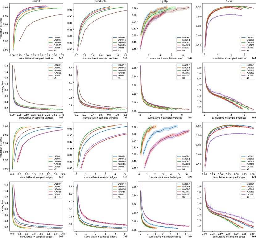
Figure 1: The validation F1-score and training loss curves on different datasets with same batch size. The x-axis stands for cumulative number of vertices and edges used during training, respectively. The soft edges represent the confidence interval. Number of sampled vertices and edges can be found in Table 2.

Table 2: Average number of vertices and edges sampled in different layers (All the numbers are in thousands, lower is better). Last two columns show iterations (mini-batches) per second (it/s) and test F1-score, for both, higher is better. The hyperparameters of LADIES and PLADIES were picked to roughly match the number of vertices sampled by the LABOR-* to get a fair comparison. The convergence curves can be found in Figure 1. The timing information was measured on an NVIDIA T4 GPU. Green stands for best, red stands for worst results, with a $5\%$ cutoff.

Dataset	Algo.	$\bm{|V^{3}|}$	$\bm{|E^{2}|}$	$\bm{|V^{2}|}$	$\bm{|E^{1}|}$	$\bm{|V^{1}|}$	$\bm{|E^{0}|}$	$\bm{|V^{0}|}$	it/s	test F1-score
	PLADIES	24	2390	14.1	927	6.0	33.2	1	1.7	96.21 $\pm$ 0.06
	LADIES	25	2270	14.5	852	6.0	32.5	1	1.8	96.20 $\pm$ 0.05
reddit	LABOR-*	24	1070	13.7	435	6.0	26.9	1	4.1	96.23 $\pm$ 0.05
	LABOR-1	27	261	14.4	116	6.1	16.7	1	24.8	96.23 $\pm$ 0.06
	LABOR-0	36	177	17.8	67	6.8	9.6	1	37.6	96.25 $\pm$ 0.05
	NS	167	682	68.3	100	10.1	9.7	1	14.2	96.24 $\pm$ 0.05
	PLADIES	160	2380	51.2	293	9.7	11.7	1	4.1	78.44 $\pm$ 0.24
	LADIES	165	2230	51.8	270	9.7	11.5	1	4.2	78.59 $\pm$ 0.22
products	LABOR-*	166	1250	51.8	167	9.8	10.6	1	6.2	78.59 $\pm$ 0.34
	LABOR-1	178	799	53.4	136	9.8	10.5	1	21.3	78.47 $\pm$ 0.26
	LABOR-0	237	615	62.4	100	10.1	9.9	1	32.5	78.76 $\pm$ 0.26
	NS	513	944	95.4	106	10.6	9.9	1	24.6	78.48 $\pm$ 0.29
	PLADIES	100	1300	29.5	183	6.2	6.9	1	5.1	61.55 $\pm$ 0.87
	LADIES	102	1280	29.7	182	6.2	6.9	1	5.3	61.89 $\pm$ 0.66
yelp	LABOR-*	105	991	30.7	158	6.1	6.8	1	13.3	61.57 $\pm$ 0.67
	LABOR-1	109	447	31.0	96	6.2	6.8	1	27.3	61.71 $\pm$ 0.70
	LABOR-0	138	318	35.1	54	6.2	6.3	1	27.2	61.55 $\pm$ 0.85
	NS	188	392	42.5	55	6.3	6.3	1	23.0	61.50 $\pm$ 0.66
	PLADIES	55	309	24.9	85	6.2	6.9	1	10.2	51.52 $\pm$ 0.26
	LADIES	56	308	25.1	85	6.2	6.9	1	10.5	50.79 $\pm$ 0.29
flickr	LABOR-*	57	308	25.6	85	6.3	6.9	1	20.3	51.67 $\pm$ 0.27
	LABOR-1	58	242	25.9	73	6.3	6.9	1	32.7	51.66 $\pm$ 0.24
	LABOR-0	66	219	29.1	52	6.4	6.7	1	33.3	51.65 $\pm$ 0.26
	NS	73	244	32.8	52	6.4	6.7	1	31.7	51.70 $\pm$ 0.23

LABOR comparison against NS:

In this experiment, we set the batch size to 1,000 and the fanout $k=10$ for LABOR and NS methods to see the difference in the sizes of the sampled subgraphs and also how vertex/edge efficient they are. In Figure 1, we can see that LABOR variants outperform NS in both vertex and edge efficiency metrics. Table 2 shows the difference of the sampled subgraph sizes in each layer. One can see that on reddit, LABOR-* samples $6.9\times$ fewer vertices in the 3rd layer leading much faster convergence in terms of cumulative number of sampled vertices. On the flickr dataset however, LABOR-* samples only $1.3\times$ fewer vertices. The amount of difference depends on two factors. The first is the amount of overlap of neighbors among the vertices in $S$. If the neighbors of vertices in $S$ did not overlap at all, then one obviously can not do better than NS. The second is the average degree of the graph. With a fanout of $10$, both NS and LABOR has to copy the whole neighborhood of a vertex $s$ with degree $d_{s}\leq 10$. Thus for such graphs, it is expected that the difference will be insignificant. The average degree of the flickr is $10.09$ (Table 1), and thus there is only a small difference between LABOR and NS.

As seen in Figure 1 and Table 2, LABOR-0 reduces both the number of vertices and edges sampled. On the other hand, when importance sampling is enabled, the number of vertices sampled goes down while number of edges sampled goes up. This is because when importance sampling is used, inclusion probabilities become nonuniform and it takes more edges per seed vertex to get a good approximation (see Equation 9). Thus, LABOR-0 leads the pack when it comes to edge efficiency.

Layer sampling algorithm comparison:

The hyperparameters of LADIES and PLADIES were picked to match LABOR-* so that all methods have the same vertex sampling budget in each layer (see Table 2). Figure 1 shows that, in terms of convergence, LADIES and PLADIES perform almost the same as each other, on all but the flickr dataset, in which case there is a big difference between the two in favor of PLADIES. We also see that LABOR variants outperform LADIES variants on products, yelp and flickr in terms of vertex efficiency with the exception of reddit, where the best performing algorithm is PLADIES proposed by us. When it comes to edge efficiency however, we see that LADIES variants are simply inefficient and all LABOR variants outperform LADIES variants on across all the datasets by up to $13\times$.

Comparing LABOR variants:

Looking at Table 2, we can see that LABOR-0 has the best runtime performance across all datasets. This is due to 1) sampling fewer edges, 2)  not having the fixed point iteration overhead, compared to the other LABOR variants. By design, all LABOR variants should have the same convergence curves, as seen in Section A.4 in Figure 3. Then, the decision of which variant to use depends on one factor: feature access speed. If vertex features were stored on a slow storage medium (such as, on host memory accessed over PCI-E), then minimizing number of sampled vertices would become the highest priority, in which case, one should pick LABOR-*. Depending on the relative vertex feature access performance and the performance of the training processor, one can choose to use LABOR-$j$, the faster feature access, the lower the $j$.

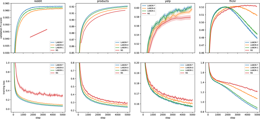
Figure 2: Validation F1-score and the training loss curves to evaluate vertex sampling efficiency under the same sampling budget. The x-axis stands for the number of training iterations. The batch size is chosen so that the # sampled vertices matches the vertex budget for each dataset and method and it is given in Table 4.

4.2 LABOR vs NS under vertex sampling budgets

In this experiment, we set a limit on the number of sampled vertices and modify the batch size to match the given vertex budget. The budgets used were picked around the same magnitude with numbers in the Table 2 in the $|V_{3}|$ column and can be found in Table 1. Figure 2 displays the result of this experiment. Table 4 shows that the more vertex efficient the sampling method is, the larger batch size it can use during training. Number of sampled vertices is not a function of the batch size for the LADIES algorithm so we do not include it in this comparison. All of the experiments were repeated 100 times and their averages were plotted, that is why our convergence plots are smooth and differences are clear. The most striking result in this experiment is that there can be up to $112\times$ difference in batch sizes of LABOR-* and NS algorithms on the reddit dataset, which translates into faster convergence as the training loss and validation F1-score curves in Figure 2 show.

Table 3: The batch sizes used in Figure 2. These were chosen such that in expectation, each method samples with the same budget given in Table 1. Having a larger batch-size speeds up convergence.

Dataset	LAB-*	LAB-1	LAB-0	NS
reddit	10100	8250	3850	90
products	7750	6000	2750	700
yelp	3700	3300	1950	1120
flickr	3600	3100	1400	800

Table 4: Number of vertices (in thousands) in 3rd layer w.r.t # fixed point iterations (its). * denotes applying the fixed point iterations until convergence, i.e., LABOR-*, 1 its stands for LABOR-1 etc.

Dataset	NS	0	1	2	3	*
reddit	167	36	27	25	25	24
products	513	237	178	170	169	166
yelp	188	138	109	106	105	105
flickr	73	66	58	57	57	56

4.3 Importance Sampling, Fixed Point Iterations

In this section, we look at the convergence behavior of the fixed point iterations described in Section 3.2.2. Table 4 shows the number of sampled vertices in the last layer with respect to the number of fixed point iterations applied. In this table, the * stands for applying the fixed point iterations until convergence, and convergence occurs in at most 15 iterations in practice before the relative change in the objective function is less than $10^{-4}$. One can see that most of the reduction in the objective function (12) occurs after the first iteration, and the remaining iterations have diminishing returns. Full convergence can save from $14\%$ - $33\%$ depending on the dataset. The monotonically decreasing numbers provide empirical evidence for the presented proof in the Section A.5.

5 Conclusions

In this paper, we introduced LABOR sampling, a novel way to combine layer and neighbor sampling approaches using a vertex-variance centric framework. We then transform the sampling problem into an optimization problem where the constraint is to match neighbor sampling variance for each vertex while sampling the fewest number of vertices. We show how to minimize this new objective function via fixed-point iterations. On datasets with dense graphs like Reddit, we show that our approach can sample a subgraph with $7\times$ fewer vertices without degrading the batch quality. We also show that compared to LADIES, LABOR converges faster with same sampling budget.

Appendix A Appendix

A.1 Derivation of Poisson Sampling variance

Following is a derivation of Equation 8 for the Horvitz-Thomson estimator. Note that we assume $\operatorname{Var}(M_{t})=1,\forall t$. Also, $\operatorname{Var}(\mathbbm{1}[r_{t}\leq\pi_{t}])$ is the variance of the bernoulli trial with probability $\pi_{t}$ and is equal to $\pi_{t}(1-\pi_{t})$.

$$H^{\prime}_{s} =\frac{1}{d_{s}}\sum_{t\to s}\frac{M_{t}}{\pi_{t}}\mathbbm{1}[r_{t}\leq\pi_{t}]$$ (19)

$$\operatorname{Var}(H^{\prime}_{s}) =\operatorname{Var}\Big{(}\frac{1}{d_{s}}\sum_{t\to s}\frac{M_{t}}{\pi_{t}}\mathbbm{1}[r_{t}\leq\pi_{t}]\Big{)}$$

$$=\frac{1}{d_{s}^{2}}\sum_{t\to s}\frac{\operatorname{Var}(M_{t})}{\pi_{t}^{2}}\operatorname{Var}(\mathbbm{1}[r_{t}\leq\pi_{t}])$$

$$=\frac{1}{d_{s}^{2}}\sum_{t\to s}\frac{\operatorname{Var}(M_{t})}{\pi_{t}^{2}}\pi_{t}(1-\pi_{t})$$

$$=\frac{1}{d_{s}^{2}}\sum_{t\to s}\frac{\operatorname{Var}(M_{t})}{\pi_{t}}(1-\pi_{t})$$

$$=\frac{1}{d_{s}^{2}}\sum_{t\to s}\frac{1}{\pi_{t}}(1-\pi_{t})$$

$$=\frac{1}{d_{s}^{2}}\sum_{t\to s}(\frac{1}{\pi_{t}}-1)$$

$$=\frac{1}{d_{s}^{2}}\sum_{t\to s}\frac{1}{\pi_{t}}-\frac{1}{d_{s}}$$

Algorithm 1 LABOR-i for uniform edge weights

  Input: seed vertices $S$, # iterations $i$, fanout $k$

  Output: sampled edges $E^{\prime}$, sampled weights $A^{\prime}$

  $T\leftarrow\{t\mid t\in N(S)\}$

  $\pi_{t}\leftarrow 1,\forall t\in T$

  while $i>0$ do

     for all $s\in S$ do

        Solve (14) for $c_{s}$

     for all $t\in T$ do

        $\pi_{t}\leftarrow\pi_{t}\max_{t\to s}c_{s}$

     $i\leftarrow i-1$

  $r_{t}\sim U(0,1),\forall t\in T$

  $E^{\prime}\leftarrow\text{[ ]}$

  $A^{\prime}\leftarrow\text{[ ]}$

  for all $s\in S$ do

     $w\leftarrow 0$

     for all $t\in N(s)$ do

        if $r_{t}\leq c_{s}\pi_{t}$ then

           $E^{\prime}$.append($t\to s$)

           $w\leftarrow w+\frac{1}{\pi_{t}}$

     for all $t\in N(s)$ do

        if $r_{t}\leq c_{s}\pi_{t}$ then

           $A^{\prime}$.append($\frac{1}{\pi_{t}w}$)

A.2 Choosing how many neighbors to sample

The variance of Poisson Sampling when $\pi_{t}=\frac{k}{d_{s}}$ is $\frac{1}{k}-\frac{1}{d_{s}}$. One might question why we are trying to match the variance of Neighbor Sampling and choose to use a fixed fanout for all the seed vertices. In the uniform probability case, if we have already sampled some set of edges for all vertices in $S$, and want to sample one more edge, the question becomes which vertex in $S$ should we sample the new edge for? Our answer to this question is the vertex $s$, whose variance would improve the most. If currently vertex $s$ has $\tilde{d}_{s}$ edges sampled, then sampling one more edge for it would improve its variance from $\frac{1}{\tilde{d}_{s}}-\frac{1}{d_{s}}$ to $\frac{1}{1+\tilde{d}_{s}}-\frac{1}{d_{s}}$. Since the derivative of the variance with respect to $\tilde{d}_{s}$ is monotonic, we are allowed to reason about the marginal improvements by comparing their derivatives, which is:

$$\frac{\partial(\frac{1}{\tilde{d}_{s}}-\frac{1}{d_{s}})}{\partial\tilde{d}_{s}}=-\frac{1}{\tilde{d}_{s}^{2}}$$ (20)

Notice that the derivative does not depend on the degree $d_{s}$ of the vertex $s$ at all, and the greater the magnitude of the derivative, the more improvement the variance of a vertex gets by sampling one more edge. Thus, choosing any vertex $s$ with least number of edges sampled would work for us, that is: $s=\operatorname*{arg\,min}_{s^{\prime}\in S}\tilde{d}_{s^{\prime}}$. In light of this observation, one can see that it is optimal to sample an equal number of edges for each vertex in $S$. This is one of the reasons LADIES is not efficient with respect to the number of edges it samples. On graphs with skewed degree distributions, it samples thousands of edges for some seed vertices, which contribute very small amounts to the variance of the estimator since it is already very close to $0$.

A.3 Sampling a fixed number of neighbors

One can easily resort to Sequential Poisson Sampling by Ohlsson [1998] if one wants $\tilde{d}_{s}=\min(k,d_{s})$ instead of $E[\tilde{d}_{s}]=\min(k,d_{s})$ to get the exact same behavior to Neighbor Sampling. Given $\pi_{t}$, $c_{s}$ and $r_{t}$, we pick the $\tilde{d}_{s}=\min(k,d_{s})$ smallest vertices $t\to s$ with respect to $\frac{r_{t}}{c_{s}\pi_{t}}$, which can be computed in expected linear time by using the quickselect algorithm [Hoare, 1961].

A.4 Baseline Comparison of Vertex/Edge Efficiency (cont.)

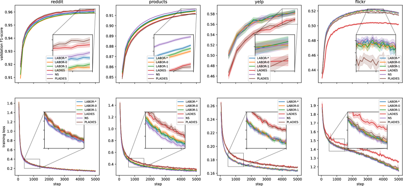
Figure 3: The validation F1-score and training loss curves on different datasets with same batch size. The soft edges represent the confidence interval. The x-axis stands for the number of training iterations. Number of sampled vertices and edges can be found in Table 2.

Here, we show another version of Figure 1, replacing the x-axis with the number of training iterations, see Figure 3. We would like to point out that despite NS and LABOR variants sampling drastically different number of vertices/edges as shown in Table 2 (up to $7\times$ fewer vertices), their convergence behavior is more or less the same, even indistinguishable on Yelp and Flickr.

A.5 Fixed point iterations

Given any $\pi^{(0)}>0$ and one iteration to get $\pi^{(1)}$ and one more iteration using $c(\pi^{(1)})$ to get $\pi^{(2)}$, then we have the following observation:

$$\pi^{(1)}_{t}=\pi^{(0)}_{t}\max_{t\to s}c_{s}(\pi^{(0)})$$

$$\frac{1}{d_{s}^{2}}\sum_{t\to s}\frac{1}{\min(1,c_{s}(\pi^{(0)})\pi^{(0)}_{t})}-\frac{1}{d_{s}}=\frac{1}{k}-\frac{1}{d_{s}}$$

$$\frac{1}{d_{s}^{2}}\sum_{t\to s}\frac{1}{\min(1,c_{s}(\pi^{(1)})\pi^{(1)}_{t})}=\frac{1}{d_{s}^{2}}\sum_{t\to s}\frac{1}{\min(1,c_{s}(\pi^{(1)})\max_{t\to s^{\prime}}c_{s^{\prime}}(\pi^{(0)})\pi^{(0)}_{t})}$$

Now, note that for a given $t\in N(s)$, $\max_{t\to s^{\prime}}c_{s^{\prime}}(\pi^{(0)})\geq c_{s}(\pi^{(0)})$ since $s\in\{s^{\prime}\mid t\to s^{\prime}\}$. This implies that $\max_{t\to s^{\prime}}c_{s^{\prime}}(\pi^{(0)})\pi^{(0)}_{t}\geq c_{s}(\pi^{(0)})\pi^{(0)}_{t}$. Note that for $\pi_{t}^{\prime}=c_{s}(\pi^{(0)})\pi^{(0)}_{t},\forall t\to s$, we have $c_{s}(\pi^{\prime})=1$ for any given $s$. Since $\max_{t\to s^{\prime}}c_{s^{\prime}}(\pi^{(0)})\pi^{(0)}_{t}\geq c_{s}(\pi^{(0)})\pi^{(0)}_{t}=\pi_{t}^{\prime},\forall t\to s$, this let’s us conclude that the $c_{s}(\pi^{(1)})\leq 1$, because the expression is monotonically increasing with respect to any of the $\pi_{t}$. By induction, this means that $c_{s}^{(i)}\leq 1,\forall i\geq 1$. Since $\pi^{(i)}_{t}=\pi^{(0)}_{t}\prod_{j=0}^{i-1}\max_{t\to s^{\prime}}c_{s^{\prime}}(\pi^{(i-1)})$, $\pi^{(i)}_{t}$ is monotonically decreasing. This means that the objective value in (12) is also monotonically decreasing and is clearly bounded from below by $0$. Any monotonically decreasing sequence bounded from below has to converge, so our fixed point iteration procedure is convergent as well.

The intuition behind the proof above is that after updating $\pi$ via (18), the probability of each edge $t\to s:\pi_{t}c_{s}$ goes up because the update takes the maximum $c_{s}$ over all possible $s$. This means each vertex gets higher quality estimators than the set variance target so we now have room to reduce the number of vertices sampled by choosing the appropriate $c_{s}\leq 1$. To summarize, $\pi$ update step increases the quality of the batch which in turn let’s the $c_{s}$ step to reduce the total number of vertices sampled.

A.6 GATv2 runtime performance

We utilize the GATv2 model Brody et al. [2022] and show the runtime performance of different samplers in Table 5. All the hyperparameters were kept same as Section 4.1 and the number of attention heads was set to 8. The runtimes correlate with the $|E_{3}|$ column in Table 2 for the GATv2 model as the computation and memory requirements depend on the number of edges. That is why the LADIES variants went out-of-memory on the reddit and products datasets.

Table 5: The runtimes (ms) per iteration for the GATv2 model on NVIDIA A100 80GB corresponding to Table 2. The abbreviation OOM stands for an ‘out-of-memory’ error, which occurs when an excessive number of edges are sampled.

Dataset	LADIES	PLADIES	LABOR-*	LABOR-1	LABOR-0	NS
reddit	OOM	OOM	266.6	69.8	51.9	155.1
products	OOM	OOM	224.8	154.6	138.7	218.5
yelp	278.0	278.9	169.2	96.6	83.2	99.5
flickr	96.6	100.3	79.8	65.0	61.1	66.2

A.7 Extension to the weighted case

If the given adjacency matrix $A$ has nonuniform weights, then we want the estimate the following:

$$H_{s}=\frac{1}{A_{*s}}\sum_{t\to s}A_{ts}M_{t}$$ (21)

where $A_{*s}=\sum_{t\to s}A_{ts}$. If we have a probability over each edge $\pi_{ts},\forall(t\to s)\in E$, then the variance becomes:

$$\operatorname{Var}(H^{\prime\prime}_{s})\leq\operatorname{Var}(nH^{\prime}_{s})=\frac{1}{(A_{*s})^{2}}\Big{(}\sum_{t\to s}\frac{A_{ts}^{2}}{\min(1,c_{s}\pi_{ts})}-\sum_{t\to s}A_{ts}^{2}\Big{)}$$ (22)

In this case, we can still aim to reach the same variance target $v_{s}=\frac{1}{k}-\frac{1}{d_{s}}$ or any given custom target $v_{s}\in\mathbb{R^{+}}$ by finding $c_{s}$ that satisfies the following equality:

$$\frac{1}{(A_{*s})^{2}}\Big{(}\sum_{t\to s}\frac{A_{ts}^{2}}{\min(1,c_{s}\pi_{ts})}-\sum_{t\to s}A_{ts}^{2}\Big{)}=v_{s}$$ (23)

In this case, the objective function becomes:

$$\pi^{*}=\operatorname*{arg\,min}_{\pi\geq 0}\sum_{t\in N(S)}\min(1,\max_{t\to s}c_{s}\pi_{ts})$$ (24)

Optimizing the objective function above will result into minimizing the number of vertices sampled. Given any $\pi_{ts}>0,\forall(t\to s)$, then the fixed point iterations proposed for the non-weighted case in (18) can be modified as follows:

$$\pi^{(0)}=A,\forall(t\to s):\pi^{(i+1)}_{ts}=\max_{t\to s^{\prime}}c_{s^{\prime}}(\pi^{(i)})\pi_{ts^{\prime}}^{(i)}$$ (25)

A more principled way to choose $v_{s}$ in the weighted case is by following the argument presented in Section A.2. There, the discussion revolves around the derivative of the variance with respect to the expected number of vertices sampled for a given seed vertex $s$. If we apply the same argument, then we get:

$$v_{s}(c_{s})=\frac{1}{(A_{*s})^{2}}\Big{(}\sum_{t\to s}\frac{A_{ts}^{2}}{\min(1,c_{s}\pi_{ts})}-\sum_{t\to s}A_{ts}^{2}\Big{)}$$

$$\frac{\partial v_{s}}{\partial c_{s}}=\frac{-1}{(A_{*s})^{2}}\sum_{t\to s}\frac{\mathbbm{1}[c_{s}\pi_{ts}<1]A_{ts}^{2}}{c_{s}^{2}\pi_{ts}}$$

$$E[\tilde{d}_{s}](c_{s})=\sum_{t\to s}\min(1,c_{s}\pi_{ts})$$

$$\frac{\partial E[\tilde{d}_{s}]}{c_{s}}=\sum_{t\to s}\mathbbm{1}[c_{s}\pi_{ts}<1]\pi_{ts}$$

Then to compute the derivative of the variance with respect to the expected number of vertices sampled for a given seed vertex $s$, which is $\frac{\partial v_{s}}{\partial E[\tilde{d}_{s}]}$, we can use the chain rule and get:

$$\frac{\partial v_{s}}{\partial E[\tilde{d}_{s}]}=\frac{\partial v_{s}}{\partial c_{s}}\frac{\partial c_{s}}{\partial E[\tilde{d}_{s}]}=\frac{\frac{-1}{(A_{*s})^{2}}\sum_{t\to s}\frac{\mathbbm{1}[c_{s}\pi_{ts}<1]A_{ts}^{2}}{c_{s}^{2}\pi_{ts}}}{\sum_{t\to s}\mathbbm{1}[c_{s}\pi_{ts}<1]\pi_{ts}}$$ (26)

Then, what one would do is to choose a constant $C(k)$ as a function of the fanout parameter $k$ and set $\frac{\partial v_{s}}{\partial E[\tilde{d}_{s}]}=C(k)$ and solve for $c_{s}$. $C(k)$ would be a negative quantity whose absolute value decreases as $k$ increases. It would probably look like $C(k)=\frac{-C^{\prime}}{k^{2}}$ for some constant $C^{\prime}>0$. We leave this as future work.

A.8 Convergence speed with respect to wall time

In this section, we perform hyperparameter optimization on Neighbor Sampler and Labor Sampler so that the training converges to a target validation accuracy as fast as possible. We leave LADIES out of this experiment because it is too slow as can be seen in the last column of Table 2. We ran this experiment on an A100 GPU and stored the input features on the main memory, which were accessed over the PCI-e directly during training by pinning their memory. This kind of training scenario is commonly used when training on large datasets whose input features don’t fit in the GPU memory. We use larger of the two datasets we have for this experiment, products and yelp. For products, the validation accuracy target we set is 91.5%, and for yelp it is 60%. We tune the learning rate between $[10^{-4},10^{-1}]$, the batch size between $[2^{10},2^{15}]$ and the fanout for each layer between $[5,25]$. We use the same model used in Section 4. For LABOR, we additionally tune over the number of importance sampling iterations i between $[0,3]$ so that it can switch between LABOR-$i$ and also a layer dependency boolean parameter that makes LABOR use the same random variates $r_{t}$ for different layers when enabled, which has the effect of increasing the overlap of sampled vertices across layers. We use the state of the art hyperparameter tuner HEBO Cowen-Rivers et al. [2020], the winning submission to the NeurIPS 2020 Black-Box Optimization Challenge, to tune the parameters of the sampling algorithm with respect to runtime required to reach the target validation accuracy with a timeout of 300 seconds, terminating the run if the configuration doesn’t reach the target accuracy.

We let HEBO run overnight and collect the minimum runtimes required to achieve the target accuracies. For products, the fastest hyperparameter corresponding to the 38.2s runtime had fanouts $(18,5,25)$, batch size $10500$, learning rate $0.0145$, used LABOR-1, layer dependency False.

For Neighbor Sampler, the fastest hyperparameter corresponding to 43.82s runtime had fanouts $(15,5,21)$, batch size $12000$, learning rate $0.0144$.

For the Yelp dataset, the fastest hyperparameter corresponding to the 41.60s runtime had fanouts $(6,5,7)$, batch size $5400$, learning rate $0.000748$, used LABOR-1 and layer dependency True.

For Neighbor Sampler, the fastest hyperparameter corresponding to the 47.40s runtime had fanouts $(5,6,6)$, batch size $4600$, learning rate $0.000931$.

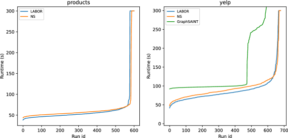
Figure 4: The runtimes to reach a validation F1-score of 91.5% on products and 60% on yelp, belonging to runs tried by the HEBO hyperparameter tuner, sorted with respect to their runtimes. Having a lower curve means that a method is faster overall compared to the others. HEBO could not find any hyperparameter configuration to reach the set target on products, hence its curve is left out.

These results clearly indicate that training with LABOR is faster compared to Neighbor Sampling when it comes to time to convergence.

We run the same experiment with GraphSAINT [Zeng et al., 2020] using the DGL example code, both on ogbn-products and yelp using the same model architecture. We used their edge sampler, the edge sampling budget between $[2^{10},2^{15}]$ and learning rate between $[10^{-4},10^{-1}]$. We disabled batch normalization to make it a fair comparison with NS and LABOR since the models they are using does not have batch normalization. We use HEBO to tune these hyperparameters to reach the set validation accuracy, and let it run overnight. The results show that HEBO was not able to find any configuration of the hyperparameters reaching 91.5% accuracy on products faster than 1500 seconds. For the Yelp dataset, the fastest runtime to reach 60% accuracy was 92.2s, with an edge sampling budget of $12500$ and learning rate $0.0214$.

References

- Bertsekas [1994] D.P. Bertsekas. Incremental least squares methods and the extended kalman filter. In Proceedings of 1994 33rd IEEE Conference on Decision and Control, volume 2, pages 1211–1214 vol.2, 1994. doi: 10.1109/CDC.1994.411166.
- Brody et al. [2022] Shaked Brody, Uri Alon, and Eran Yahav. How attentive are graph attention networks? In International Conference on Learning Representations, 2022. URL https://openreview.net/forum?id=F72ximsx7C1.
- Chen et al. [2018a] Jianfei Chen, Jun Zhu, and Le Song. Stochastic training of graph convolutional networks with variance reduction. 35th International Conference on Machine Learning, ICML 2018, 3:1503–1532, 2018a.
- Chen et al. [2018b] Jie Chen, Tengfei Ma, and Cao Xiao. FastGCN: Fast Learning with Graph Convolutional Networks via Importance Sampling. jan 2018b. URL http://arxiv.org/abs/1801.10247.
- Chen et al. [2022] Yifan Chen, Tianning Xu, Dilek Hakkani-Tur, Di Jin, Yun Yang, and Ruoqing Zhu. Calibrate and Debias Layer-wise Sampling for Graph Convolutional Networks. jun 2022. URL http://arxiv.org/abs/2206.00583.
- Chiang et al. [2019] Wei Lin Chiang, Yang Li, Xuanqing Liu, Samy Bengio, Si Si, and Cho Jui Hsieh. Cluster-GCN: An efficient algorithm for training deep and large graph convolutional networks. In Proceedings of the ACM SIGKDD International Conference on Knowledge Discovery and Data Mining, pages 257–266. Association for Computing Machinery, jul 2019. doi: 10.1145/3292500.3330925.
- Ching et al. [2015] Avery Ching, Sergey Edunov, Maja Kabiljo, Dionysios Logothetis, and Sambavi Muthukrishnan. One trillion edges: Graph processing at facebook-scale. Proc. VLDB Endow., 8(12):1804–1815, aug 2015. doi: 10.14778/2824032.2824077. URL https://doi.org/10.14778/2824032.2824077.
- Cong et al. [2021] Weilin Cong, Morteza Ramezani, and Mehrdad Mahdavi. On the Importance of Sampling in Training GCNs: Tighter Analysis and Variance Reduction. 2021. URL http://arxiv.org/abs/2103.02696.
- Cowen-Rivers et al. [2020] Alexander I Cowen-Rivers, Wenlong Lyu, Rasul Tutunov, Zhi Wang, Antoine Grosnit, Ryan Rhys Griffiths, Hao Jianye, Jun Wang, and Haitham Bou Ammar. An empirical study of assumptions in bayesian optimisation. arXiv preprint arXiv:2012.03826, 2020.
- Dong et al. [2021] Jialin Dong, Da Zheng, Lin F. Yang, and George Karypis. Global Neighbor Sampling for Mixed CPU-GPU Training on Giant Graphs. Proceedings of the ACM SIGKDD International Conference on Knowledge Discovery and Data Mining, pages 289–299, 2021. doi: 10.1145/3447548.3467437.
- Dorfman [1997] Alan H Dorfman. The Hajek Estimator Revisited. (4):760–765, 1997. URL http://www.asasrms.org/Proceedings/papers/1997_130.pdf.
- Fey and Lenssen [2019] Matthias Fey and Jan Eric Lenssen. Fast graph representation learning with pytorch geometric, 2019. URL https://arxiv.org/abs/1903.02428.
- Fey et al. [2021] Matthias Fey, Jan E. Lenssen, Frank Weichert, and Jure Leskovec. Gnnautoscale: Scalable and expressive graph neural networks via historical embeddings. In Marina Meila and Tong Zhang, editors, Proceedings of the 38th International Conference on Machine Learning, volume 139 of Proceedings of Machine Learning Research, pages 3294–3304. PMLR, 18–24 Jul 2021. URL https://proceedings.mlr.press/v139/fey21a.html.
- Hamilton et al. [2017] Will Hamilton, Zhitao Ying, and Jure Leskovec. Inductive representation learning on large graphs. In I. Guyon, U. Von Luxburg, S. Bengio, H. Wallach, R. Fergus, S. Vishwanathan, and R. Garnett, editors, Advances in Neural Information Processing Systems, volume 30. Curran Associates, Inc., 2017. URL https://proceedings.neurips.cc/paper/2017/file/5dd9db5e033da9c6fb5ba83c7a7ebea9-Paper.pdf.
- Hoare [1961] C. A. R. Hoare. Algorithm 65: Find. Commun. ACM, 4(7):321–322, jul 1961. doi: 10.1145/366622.366647. URL https://doi.org/10.1145/366622.366647.
- Hu et al. [2020a] Weihua Hu, Matthias Fey, Marinka Zitnik, Yuxiao Dong, Hongyu Ren, Bowen Liu, Michele Catasta, and Jure Leskovec. Open graph benchmark: Datasets for machine learning on graphs. Advances in Neural Information Processing Systems, 2020-Decem(NeurIPS):1–34, 2020a.
- Hu et al. [2020b] Ziniu Hu, Yuxiao Dong, Kuansan Wang, and Yizhou Sun. Heterogeneous Graph Transformer. The Web Conference 2020 - Proceedings of the World Wide Web Conference, WWW 2020, pages 2704–2710, 2020b. doi: 10.1145/3366423.3380027.
- Huang et al. [2018] Wenbing Huang, Tong Zhang, Yu Rong, and Junzhou Huang. Adaptive sampling towards fast graph representation learning. Advances in Neural Information Processing Systems, 2018-Decem(Nips):4558–4567, 2018.
- Khan and Ugander [2021] Samir Khan and Johan Ugander. Adaptive normalization for IPW estimation. pages 1–31, 2021. URL http://arxiv.org/abs/2106.07695.
- Kingma and Ba [2014] Diederik P. Kingma and Jimmy Ba. Adam: A method for stochastic optimization, 2014. URL https://arxiv.org/abs/1412.6980.
- Kipf and Welling [2017] Thomas N. Kipf and Max Welling. Semi-supervised classification with graph convolutional networks. 5th International Conference on Learning Representations, ICLR 2017 - Conference Track Proceedings, pages 1–14, 2017.
- Liu et al. [2020] Ziqi Liu, Zhengwei Wu, Zhiqiang Zhang, Jun Zhou, Shuang Yang, Le Song, and Yuan Qi. Bandit samplers for training graph neural networks. Advances in Neural Information Processing Systems, 2020-Decem, 2020.
- Niu et al. [2020] Xichuan Niu, Bofang Li, Chenliang Li, Rong Xiao, Haochuan Sun, Hongbo Deng, and Zhenzhong Chen. A dual heterogeneous graph attention network to improve long-tail performance for shop search in e-commerce. In Proceedings of the 26th ACM SIGKDD International Conference on Knowledge Discovery and Data Mining, KDD ’20, page 3405–3415, 2020. doi: 10.1145/3394486.3403393.
- Ohlsson [1998] E Ohlsson. Sequential poisson sampling. Journal of Official Statistics-Stockholm-, 14(2):149–162, 1998.
- Paszke et al. [2019] Adam Paszke, Sam Gross, Francisco Massa, Adam Lerer, James Bradbury, Gregory Chanan, Trevor Killeen, Zeming Lin, Natalia Gimelshein, Luca Antiga, Alban Desmaison, Andreas Köpf, Edward Yang, Zach DeVito, Martin Raison, Alykhan Tejani, Sasank Chilamkurthy, Benoit Steiner, Lu Fang, Junjie Bai, and Soumith Chintala. Pytorch: An imperative style, high-performance deep learning library. In NeurIPS, 2019.
- Shi et al. [2023] Zhihao Shi, Xize Liang, and Jie Wang. LMC: Fast training of GNNs via subgraph sampling with provable convergence. In The Eleventh International Conference on Learning Representations, 2023. URL https://openreview.net/forum?id=5VBBA91N6n.
- Wang et al. [2019] Minjie Wang, Da Zheng, Zihao Ye, Quan Gan, Mufei Li, Xiang Song, Jinjing Zhou, Chao Ma, Lingfan Yu, Yu Gai, Tianjun Xiao, Tong He, George Karypis, Jinyang Li, and Zheng Zhang. Deep graph library: A graph-centric, highly-performant package for graph neural networks, 2019. URL https://arxiv.org/abs/1909.01315.
- Williams et al. [1998] Michael S Williams, Hans T Schreuder, and Gerardo H Terrazas. Poisson Sampling – The Adjusted and Unadjusted Estimator Revisited. page 12, 1998.
- Ying et al. [2018] Rex Ying, Ruining He, Kaifeng Chen, Pong Eksombatchai, William L. Hamilton, and Jure Leskovec. Graph convolutional neural networks for web-scale recommender systems. Proceedings of the ACM SIGKDD International Conference on Knowledge Discovery and Data Mining, pages 974–983, 2018. doi: 10.1145/3219819.3219890.
- Zeng et al. [2020] Hanqing Zeng, Hongkuan Zhou, Ajitesh Srivastava, Rajgopal Kannan, and Viktor Prasanna. GraphSAINT: Graph sampling based inductive learning method. In International Conference on Learning Representations, 2020. URL https://openreview.net/forum?id=BJe8pkHFwS.
- Zeng et al. [2021] Hanqing Zeng, Muhan Zhang, Yinglong Xia, Ajitesh Srivastava, Andrey Malevich, Rajgopal Kannan, Viktor Prasanna, Long Jin, and Ren Chen. Decoupling the depth and scope of graph neural networks. In A. Beygelzimer, Y. Dauphin, P. Liang, and J. Wortman Vaughan, editors, Advances in Neural Information Processing Systems, 2021. URL https://openreview.net/forum?id=d0MtHWY0NZ.
- Zhang et al. [2021] Qingru Zhang, David Wipf, Quan Gan, and Le Song. A Biased Graph Neural Network Sampler with Near-Optimal Regret. (NeurIPS):1–25, 2021. URL http://arxiv.org/abs/2103.01089.
- Zheng et al. [2022a] Che Zheng, Hongzhi Chen, Yuxuan Cheng, Zhezheng Song, Yifan Wu, Changji, Li, James Cheng, Han Yang, and Shuai Zhang. Bytegnn: Efficient graph neural network training at large scale. Proc. VLDB Endow., 15:1228–1242, 2022a.
- Zheng et al. [2022b] Da Zheng, Xiang Song, Chengru Yang, Dominique LaSalle, and George Karypis. Distributed hybrid cpu and gpu training for graph neural networks on billion-scale heterogeneous graphs. In Proceedings of the 28th ACM SIGKDD Conference on Knowledge Discovery and Data Mining, pages 4582–4591, 2022b.
- Zou et al. [2019] Difan Zou, Ziniu Hu, Yewen Wang, Song Jiang, Yizhou Sun, and Quanquan Gu. Layer-dependent importance sampling for training deep and large graph convolutional networks. Advances in Neural Information Processing Systems, 32(NeurIPS), 2019.