1 Introduction

Let $\mathbb{R}^{m}$ and $\mathbb{R}^{n}$ be finite-dimensional Euclidean spaces and assume that the function $f:\mathbb{R}^{m}\times\mathbb{R}^{n}\mapsto\mathbb{R}$ has a bounded and Lipschitz-continuous Hessian. We consider the problem of finding a global saddle point of the following min-max optimization problem:

$$\min_{\mathbf{x}\in\mathbb{R}^{m}}\max_{\mathbf{y}\in\mathbb{R}^{n}}\ f(\mathbf{x},\mathbf{y}),$$ (1.1)

i.e., a tuple $(\mathbf{x}^{\star},\mathbf{y}^{\star})\in\mathbb{R}^{m}\times\mathbb{R}^{n}$ such that

$$f(\mathbf{x}^{\star},\mathbf{y})\leq f(\mathbf{x}^{\star},\mathbf{y}^{\star})\leq f(\mathbf{x},\mathbf{y}^{\star}),\quad\textnormal{for all }\mathbf{x}\in\mathbb{R}^{m},\ \mathbf{y}\in\mathbb{R}^{n}.$$

Throughout our paper, we assume that the function $f(\mathbf{x},\mathbf{y})$ is convex in $\mathbf{x}$ for all $\mathbf{y}\in\mathbb{R}^{n}$ and concave in $\mathbf{y}$ for all $\mathbf{x}\in\mathbb{R}^{m}$. This convex-concave setting has been the focus of intense research in optimization, game theory, economics and computer science for several decades now (Von Neumann and Morgenstern, 1953; Dantzig, 1963; Blackwell and Girshick, 1979; Facchinei and Pang, 2007; Ben-Tal et al., 2009), and variants of the problem have recently attracted significant interest in machine learning and data science, with applications in generative adversarial networks (GANs) (Goodfellow et al., 2014; Arjovsky et al., 2017), adversarial learning (Sinha et al., 2018), distributed multi-agent systems (Shamma, 2008), and many other fields; for a range of concrete examples, see Facchinei and Pang (2007) and references therein.

Motivated by these applications, several classes of optimization algorithms have been proposed and analyzed for finding a global saddle point of Eq. (1.1) in the convex-concave case. An important algorithm is the extragradient (EG) method (Korpelevich, 1976; Antipin, 1978; Nemirovski, 2004). The method’s rate of convergence for smooth and strongly-convex-strongly-concave functions and bilinear functions (i.e., when $f(\mathbf{x},\mathbf{y})=\mathbf{x}^{\top}A\mathbf{y}$ for some square, full-rank matrix $A$) was shown to be linear by Korpelevich (1976) and Tseng (1995). Subsequently, Nemirovski (2004) showed that the method enjoys an $O(\epsilon^{-1})$ convergence guarantee for constrained problems with a bounded domain and a convex-concave function $f$. In unbounded domains, Solodov and Svaiter (1999) generalized EG to the hybrid proximal extragradient (HPE) method which provides a framework for analyzing the iteration complexity of several existing algorithms, including EG and Tseng’s forward-backward splitting (Tseng, 2000), while Monteiro and Svaiter (2010) provided an $O(\epsilon^{-1})$ guarantee for HPE in both bounded and unbounded domains. In addition to EG, there are other methods that can achieve the same convergence guarantees, such as optimistic gradient descent ascent (OGDA) (Popov, 1980) and dual extrapolation (DE) (Nesterov, 2007); for a partial survey, see Hsieh et al. (2019) and the references therein. All these methods are order-optimal first-order methods since they have matched the lower bound of Ouyang and Xu (2021).

Focusing on convex minimization problems for the moment, significant effort has been devoted to developing first-order methods that are characterized by simplicity of implementation and analytic tractability (Nesterov, 1983; Beck and Teboulle, 2009). In particular, it has been recognized that first-order methods are suitable for solving large-scale machine learning problems where low-accuracy solutions may suffice (Sra et al., 2012; Lan, 2020). However, second-order methods are known to enjoy superior convergence properties over their first-order counterparts, in both theory and practice for many other problems. For instance, the accelerated cubic regularized Newton method (Nesterov, 2008) and accelerated Newton proximal extra-gradient method (Monteiro and Svaiter, 2013) converge at a rate of $O(\epsilon^{-1/3})$ and $\tilde{O}(\epsilon^{-2/7})$ respectively, both exceeding the best possible $O(\epsilon^{-1/2})$ bound for first-order methods (Nemirovski and Yudin, 1983). Optimal second-order methods with the rate of $O(\epsilon^{-2/7})$ were further recently proposed by Carmon et al. (2022) and Kovalev and Gasnikov (2022). Moreover, first-order methods may perform poorly in ill-conditioned problems and can be sensitive to the parameter choices in real-world applications in which second-order methods are observed to be more robust (Pilanci and Wainwright, 2017; Roosta-Khorasani and Mahoney, 2019; Berahas et al., 2020).

By contrast, in the context of convex-concave min-max problems, two separate issues arise: (a) achieving acceleration with second-order information is much less tractable analytically; and (b) acquiring accurate second-order information is computationally very expensive in general. Aiming to address these issues, a line of recent work has generalized classical first-order methods, e.g., EG and OGDA, to their higher-order counterparts (Monteiro and Svaiter, 2012; Bullins and Lai, 2022; Jiang and Mokhtari, 2022; Lin and Jordan, 2023), where the best known upper bound is $O(\epsilon^{-2/3}\log\log(1/\epsilon))$ (Jiang and Mokhtari, 2022) with a lower bound of $\Omega(\epsilon^{-2/3})$ (Lin and Jordan, 2022; Adil et al., 2022). Closing this $\log\log(1/\epsilon)$ gap is not only of theoretical interest but has important practical implications because all existing methods require solving a nontrivial implicit binary search problem at each iteration, and this can be computationally expensive in practice.

Working in a similar vein,  Huang et al. (2022) extended cubic regularized Newton methods (Nesterov and Polyak, 2006) to convex-concave min-max optimization. The algorithm of Huang et al. (2022) has two phases and the guarantees provided therein require a certain error bound condition with a parameter $\theta\in(0,1]$ (Huang et al., 2022, Assumption 5.1). Indeed, the rate is linear under a Lipschitz-type condition ($\theta=1$) and $O(\epsilon^{-(1-\theta)/\theta^{2}})$ under a Hölder-type condition ($\theta\in(0,1)$). These conditions unfortunately exclude some important problem classes and are hard to be verified in practice. Focusing on solving more general monotone variational inequalities, Nesterov (2006) also extended the cubic regularized Newton’s method and proved a global convergence rate of $O(\epsilon^{-1})$.

Fianally, it is also worth mentioning that existing second-order min-max optimization algorithms require exact second-order information; as a result, given the implicit nature of the inner loop subproblems involved, the methods’ robustness to inexact information cannot be taken for granted. It is thus natural to ask:

Can we develop explicit second-order min-max optimization algorithms that remain order-optimal even with inexact second-order information?

Our paper provides an affirmative answer to this question. In particular, inspired by recent advances in the literature on variational inequalities (VIs) (Lin and Jordan, 2022), we begin by proposing a conceptual second-order min-max optimization algorithm with a global convergence guarantee of $O(\epsilon^{-2/3})$ in the convex-concave case. The proposed algorithm does not contain any binary search procedure but still requires exact second-order information and an exact solution of an inner explicit subproblem. Subsequently, to relax these requirements, we propose a class of second-order min-max optimization algorithms that only require inexact second-order information and inexact subproblem solutions. The approximation condition is inspired by Condition 1 in Xu et al. (2020) and allows for direct construction of such oracles through randomized sampling in the case of finite-sum problems (Drineas and Mahoney, 2018). As far as we are aware, this is the first class of subsampled Newton methods for solving finite-sum min-max optimization problems, gaining considerable computational savings since the sample size increases gracefully from a very small sample set. In terms of theoretical guarantees, we prove that these inexact algorithms achieve the convergence guarantee of $O(\epsilon^{-2/3})$ and the subsampled Newton methods achieve the same rate with high probability.

Overall, our paper stands at the interface of two synergistic research thrusts in the literature: one is to generalize second-order methods for convex minimization problems (Huang et al., 2022) and the other is to generalize first-order methods for min-max optimization problems (Monteiro and Svaiter, 2012; Bullins and Lai, 2022; Jiang and Mokhtari, 2022; Lin and Jordan, 2023). To the best of our knowledge, there are no explicit second-order methods in the literature that (i) achieve an order-optimal convergence guarantee of $\Theta(\epsilon^{-2/3})$ in the convex-concave case; and (ii) do not require exact second-order information in their implementation. Experimental results on both real and synthetic data demonstrate the efficiency of the proposed algorithms.

1.1 Related Work

Our work comes amid a surge of interest in optimization algorithms for a large class of emerging min-max optimization problems. For brevity, we will focus on the convex-concave cases and leave other cases out of discussion; see Section 2 in Lin et al. (2020) for a more detailed presentation.

Historically, a concrete instantiation of the convex-concave min-max optimization problem is the solution of $\min_{\mathbf{x}\in\Delta^{m}}\max_{\mathbf{y}\in\Delta^{n}}\mathbf{x}^{\top}A\mathbf{y}$ for $A\in\mathbb{R}^{m\times n}$ over the simplices $\Delta^{m}$ and $\Delta^{n}$. Spurred by von Neumann’s theorem (Neumann, 1928), this problem provided the initial impetus for min-max optimization. Sion (1958) generalized von Neumann’s result from bilinear cases to convex-concave cases and triggered a line of research on algorithms for convex-concave min-max optimization (Korpelevich, 1976; Nemirovski, 2004; Nesterov, 2007; Nedić and Ozdaglar, 2009; Mokhtari et al., 2020b). A notable result is that gradient descent ascent (GDA) with diminishing stepsizes can find an $\epsilon$-global saddle point within $O(\epsilon^{-2})$ iterations if the gradients are bounded over the feasible sets (Nedić and Ozdaglar, 2009).

Recent years have witnessed progress on the analysis of first-order min-max optimization algorithms in bilinear cases and convex-concave cases. In the bilinear case, Daskalakis et al. (2018) proved the convergence of OGDA to a neighborhood of a global saddle point. Liang and Stokes (2019) used a dynamical system approach to establish the linear convergence of OGDA for the special case when the matrix $A$ is square and full rank. Mokhtari et al. (2020a) have revisited proximal point method and proposed an unified framework for achieving the sharpest convergence rates of both EG and OGDA. In the convex-concave case, Nemirovski (2004) demonstrated that EG finds an $\epsilon$-global saddle point within $O(\epsilon^{-1})$ iterations when the feasible sets are convex and compact. The same convergence guarantee was extended to unbounded feasible sets (Monteiro and Svaiter, 2010, 2011) using the HPE algorithm with different optimality criteria. Nesterov (2007) and Tseng (2008) proposed new algorithms and refined convergence analysis with the same convergence guarantee. Abernethy et al. (2021) presented a Hamiltonian gradient descent method with last-iterate convergence under a “sufficiently bilinear” condition. Focusing on special min-max optimization problems with $f(\mathbf{x},\mathbf{y})=g(\mathbf{x})+\mathbf{x}^{\top}A\mathbf{y}-h(\mathbf{y})$, Chambolle and Pock (2011) introduced a primal-dual hybrid gradient algorithm that converges to a global saddle point at the rate of $O(\epsilon^{-1})$ when the functions $g$ and $h$ are simple and convex. Nesterov (2005) proposed a smoothing technique and proved that his algorithm achieves better dependence on problem parameters for convex and compact constraint sets. He and Monteiro (2016) and Kolossoski and Monteiro (2017) proved that such a result still holds for unbounded feasible sets and non-Euclidean metrics. Moreover, Chen et al. (2014) developed optimal algorithms for solving min-max optimization problems with $f(\mathbf{x},\mathbf{y})=g(\mathbf{x})+\mathbf{x}^{\top}A\mathbf{y}-h(\mathbf{y})$ even when only noisy gradients are available.

Compared to first-order methods, there has been less research on second-order methods for min-max optimization problems with global convergence rate guarantee. In this regard, we are only aware of two above research thrusts (Monteiro and Svaiter, 2012; Bullins and Lai, 2022; Jiang and Mokhtari, 2022; Huang et al., 2022; Adil et al., 2022; Lin and Jordan, 2022, 2023). Although our exact method (Algorithm 1) is inspired by the variational inequality method of Lin and Jordan (2022) for unconstrained min-max optimization problems, our analysis is not a simple extension thereof: the non-compact setting requires a different Lyapunov-type approach – cf. Eq. (3.3) later on – which, in addition to handling unbounded domains and operators, is more intuitive than that of Lin and Jordan (2022) and allows us to obtain a more streamlined, unified proof template for second-order methods, By contrast, the boundedness condition is deeply ingrained in the analysis of Lin and Jordan (2022) – cf. Eq. (9) therein and the surrounding discussion – and there is no straightforward modification that could handle even a subsequence of iterates potentially escaping to infinity. In this regard, and to the best of our knowledge, our paper seems to be the first to achieve the order-optimal convergence rate of $O(\epsilon^{-2/3})$ in unconstrained second-order min-max optimization under a restricted primal-dual gap function and is the first to consider subsampling strategies in this setting. As far as we are aware, the complexity bound guarantees of Algorithms 2 and 3 cannot be realized by all existing second-order min-max optimization methods with exact second-order oracle requirements.

1.2 Notation and Organization

We use bold lower-case letters to denote vectors, as in $\mathbf{x},\mathbf{y},\mathbf{z}$. For a function $f(\cdot):\mathbb{R}^{n}\rightarrow\mathbb{R}$, we let $\nabla f(\mathbf{z})$ denote the gradient of $f$ at $\mathbf{z}$. For a function $f(\cdot,\cdot):\mathbb{R}^{m}\times\mathbb{R}^{n}\rightarrow\mathbb{R}$ of two variables, $\nabla_{\mathbf{x}}f(\mathbf{x},\mathbf{y})$ (or $\nabla_{\mathbf{y}}f(\mathbf{x},\mathbf{y})$) to denote the partial gradient of $f$ with respect to the first variable (or the second variable) at point $(\mathbf{x},\mathbf{y})$. We use $\nabla f(\mathbf{x},\mathbf{y})$ to denote the full gradient at $(\mathbf{x},\mathbf{y})$ where $\nabla f(\mathbf{x},\mathbf{y})=(\nabla_{\mathbf{x}}f(\mathbf{x},\mathbf{y}),\nabla_{\mathbf{y}}f(\mathbf{x},\mathbf{y}))$ and $\nabla^{2}f(\mathbf{x},\mathbf{y})$ to denote the full Hessian at $(\mathbf{x},\mathbf{y})$. For a vector $\mathbf{x}$, we write $\|\mathbf{x}\|$ for its $\ell_{2}$-norm. Finally, we use $O(\cdot),\Omega(\cdot)$ to hide absolute constants which do not depend on any problem parameter, and $\tilde{O}(\cdot),\tilde{\Omega}(\cdot)$ to hide absolute constants and log factors.

The remainder of the paper is organized as follows. In Section 2, we present the setup of smooth min-max optimization and provide the definitions for functions and optimality criteria. In Section 3, we propose an exact second-order min-max optimization algorithm without any binary search procedure and prove that it achieves a global convergence rate of $O(\epsilon^{-2/3})$ in the convex-concave case. In Section 4, we propose a broad class of second-order min-max optimization algorithms under inexact second-order information and inexact subproblem solving and prove the same convergence guarantee. We also provide the subsampled Newton method for solving the finite-sum min-max optimization problems. In Section 5, we conduct the experiments on synthetic and real data to demonstrate the efficiency of our algorithms.

2 Preliminaries

We present the basic setup of min-max problems under study, and we provide the definitions for the optimality criteria considered in the sequel. In this regard, the regularity conditions that we impose for the function $f:\mathbb{R}^{m+n}\mapsto\mathbb{R}$ are as follows:

Definition 2.1

A function $f$ is $\rho$-Hessian Lipschitz if $\|\nabla^{2}f(\mathbf{z})-\nabla^{2}f(\mathbf{z}^{\prime})\|\leq\rho\|\mathbf{z}-\mathbf{z}^{\prime}\|$ for all $\mathbf{z},\mathbf{z}^{\prime}\in\mathbb{R}^{n}$.

Definition 2.2

A differentiable function $f$ is convex-concave if

$$\begin{array}[]{rl}f(\mathbf{x}^{\prime},\mathbf{y})\geq f(\mathbf{x},\mathbf{y})+(\mathbf{x}^{\prime}-\mathbf{x})^{\top}\nabla_{\mathbf{x}}f(\mathbf{x},\mathbf{y}),&\textnormal{for }\mathbf{x}^{\prime},\mathbf{x}\in\mathbb{R}^{m}\textnormal{ and any fixed }\mathbf{y}\in\mathbb{R}^{n},\\ f(\mathbf{x},\mathbf{y}^{\prime})\leq f(\mathbf{x},\mathbf{y})+(\mathbf{y}^{\prime}-\mathbf{y})^{\top}\nabla_{\mathbf{x}}f(\mathbf{x},\mathbf{y}),&\textnormal{for }\mathbf{y}^{\prime},\mathbf{y}\in\mathbb{R}^{n}\textnormal{ and any fixed }\mathbf{x}\in\mathbb{R}^{m}.\end{array}$$

We also define the notion of global saddle points for the min-max problem in Eq. (1.1).

Definition 2.3

A point $(\mathbf{x}^{\star},\mathbf{y}^{\star})\in\mathbb{R}^{m}\times\mathbb{R}^{n}$ is a global saddle point of a convex-concave function $f(\cdot,\cdot)$ if $f(\mathbf{x}^{\star},\mathbf{y})\leq f(\mathbf{x}^{\star},\mathbf{y}^{\star})\leq f(\mathbf{x},\mathbf{y}^{\star})$ for all $\mathbf{x}\in\mathbb{R}^{m}$ and $\mathbf{y}\in\mathbb{R}^{n}$.

Throughout this paper, we will assume that the following conditions are satisfied.

Assumption 2.4

The function $f(\mathbf{x},\mathbf{y})$ is continuously differentiable. Further, the function $f(\mathbf{x},\mathbf{y})$ is a convex function of $\mathbf{x}$ for any $\mathbf{y}\in\mathbb{R}^{n}$ and a concave function of $\mathbf{y}$ for any $\mathbf{x}\in\mathbb{R}^{m}$. There also exists at least one global saddle point of $f(\mathbf{x},\mathbf{y})$ for the min-max problem in Eq. (1.1).

Assumption 2.5

The function $f(\mathbf{x},\mathbf{y}):\mathbb{R}^{m}\times\mathbb{R}^{n}\mapsto\mathbb{R}$ is $\rho$-Hessian Lipschitz. Formally, we have

$$\|\nabla^{2}f(\mathbf{x},\mathbf{y})-\nabla^{2}f(\mathbf{x}^{\prime},\mathbf{y}^{\prime})\|\leq\rho\left\|\begin{bmatrix}\mathbf{x}-\mathbf{x}^{\prime}\\ \mathbf{y}-\mathbf{y}^{\prime}\end{bmatrix}\right\|,\quad\textnormal{for all }(\mathbf{x},\mathbf{y}),(\mathbf{x}^{\prime},\mathbf{y}^{\prime})\in\mathbb{R}^{m}\times\mathbb{R}^{n}.$$

Under Assumption 2.4, we clearly have $f(\mathbf{x}^{\star},\mathbf{y})\leq f(\mathbf{x}^{\star},\mathbf{y}^{\star})\leq f(\mathbf{x},\mathbf{y}^{\star})$ for all $\mathbf{x}\in\mathbb{R}^{m}$ and $\mathbf{y}\in\mathbb{R}^{n}$. This leads to the notion of a restricted gap function (Nesterov, 2007) which provides a performance measure for the closeness of $(\hat{\mathbf{x}},\hat{\mathbf{y}})$ to a global saddle point $(\mathbf{x}^{\star},\mathbf{y}^{\star})$ in the unconstrained convex-concave setting. Indeed, we let $\beta>0$ be sufficiently large such that $\max\{\|\hat{\mathbf{x}}-\mathbf{x}^{\star}\|,\|\hat{\mathbf{y}}-\mathbf{y}^{\star}\|\}\leq\beta$ and define the restricted gap function $\mathrm{Gap}(\hat{\mathbf{x}},\hat{\mathbf{y}};\beta)=\max_{\mathbf{y}\in\mathbb{B}_{\beta}(\mathbf{y}^{\star})}f(\hat{\mathbf{x}},\mathbf{y})-\min_{\mathbf{x}\in\mathbb{B}_{\beta}(\mathbf{x}^{\star})}f(\mathbf{x},\hat{\mathbf{y}})$. It is clear here that $\mathrm{Gap}(\hat{\mathbf{x}},\hat{\mathbf{y}};\beta)\geq 0$ since $f(\mathbf{x}^{\star},\hat{\mathbf{y}})\leq f(\hat{\mathbf{x}},\mathbf{y}^{\star})$ holds true. Formally, we have the following definition.

Definition 2.6

A point $(\hat{\mathbf{x}},\hat{\mathbf{y}})\in\mathbb{R}^{m}\times\mathbb{R}^{n}$ is an $\epsilon$-global saddle point of a convex-concave function $f(\cdot,\cdot)$ if $\mathrm{Gap}(\hat{\mathbf{x}},\hat{\mathbf{y}};\beta)\leq\epsilon$. If $\epsilon=0$, we have that $(\hat{\mathbf{x}},\hat{\mathbf{y}})$ is a global saddle point of the function $f(\cdot,\cdot)$.

In the subsequent sections, we propose a new regularized Newton method for solving the min-max optimization problem in Eq. (1.1) and prove an optimal global convergence rate in the sense that our upper bound on the required iteration number to return an $\epsilon$-optimal solution matches the lower bound.

In our algorithm, we denote the $k^{\textnormal{th}}$ iterate by $(\mathbf{x}_{k},\mathbf{y}_{k})$ and we define the averaged (ergodic) iterates by $(\bar{\mathbf{x}}_{k},\bar{\mathbf{y}}_{k})$. In particular, given a sequence of weights $\{\lambda_{n}\}_{n=1}^{T}$, we let

$$\bar{\mathbf{x}}_{k}=\tfrac{1}{\sum_{i=1}^{k}\lambda_{i}}\left(\sum_{i=1}^{k}\lambda_{i}\mathbf{x}_{i}\right),\quad\bar{\mathbf{y}}_{k}=\tfrac{1}{\sum_{i=1}^{k}\lambda_{i}}\left(\sum_{i=1}^{k}\lambda_{i}\mathbf{y}_{i}\right).$$ (2.1)

In our convergence analysis, we define the vector $\mathbf{z}=[\mathbf{x};\mathbf{y}]\in\mathbb{R}^{m+n}$ and the operator $F:\mathbb{R}^{m+n}\mapsto\mathbb{R}^{m+n}$ as follows,

$$F(\mathbf{z})=\begin{bmatrix}\nabla_{\mathbf{x}}f(\mathbf{x},\mathbf{y})\\ -\nabla_{\mathbf{y}}f(\mathbf{x},\mathbf{y})\end{bmatrix}.$$ (2.2)

Accordingly, the Jacobian of $F$ is defined as follows (note that $DF$ is asymmetric in general),

$$DF(\mathbf{z})=\begin{bmatrix}\nabla^{2}_{\textbf{xx}}f(\mathbf{x},\mathbf{y})&\nabla^{2}_{\textbf{xy}}f(\mathbf{x},\mathbf{y})\\ -\nabla^{2}_{\textbf{xy}}f(\mathbf{x},\mathbf{y})&-\nabla^{2}_{\textbf{yy}}f(\mathbf{x},\mathbf{y})\end{bmatrix}\in\mathbb{R}^{(m+n)\times(m+n)}.$$ (2.3)

In the following lemma, we summarize the properties of the operator $F$ in Eq. (2.2) and its Jacobian in Eq. (2.3) under Assumption 2.4 and 2.5. We note that most of the results in the following lemma are well known (Nemirovski, 2004) so we omit their proofs.

Lemma 2.7

Let $F(\cdot)$ and $DF(\cdot)$ be defined as above and Assumptions 2.4 and 2.5 hold true. Then, we have

• $F$ is monotone, i.e., $(\mathbf{z}-\mathbf{z}^{\prime})^{\top}(F(\mathbf{z})-F(\mathbf{z}^{\prime}))\geq 0$.

• $DF$ is $\rho$-Lipschitz continuous, i.e., $\|DF(\mathbf{z})-DF(\mathbf{z}^{\prime})\|\leq\rho\|\mathbf{z}-\mathbf{z}^{\prime}\|$.

• $F(\mathbf{z}^{\star})=0$ for any global saddle point $\mathbf{z}^{\star}\in\mathbb{R}^{m+n}$ of the function $f(\cdot,\cdot)$.

Proof. Note that (a) and (c) have been proven in earlier work (Nemirovski, 2004), and it suffices to prove (b). By using the definition of $DF(\cdot)$ in Eq. (2.3), we have

$$(DF(\mathbf{z})-DF(\mathbf{z}^{\prime}))\mathbf{h}=\begin{bmatrix}I_{m}&\\ &-I_{n}\end{bmatrix}(\nabla^{2}f(\mathbf{z})-\nabla^{2}f(\mathbf{z}^{\prime}))\mathbf{h}.$$ (2.4)

This implies that $\|(DF(\mathbf{z})-DF(\mathbf{z}^{\prime}))\mathbf{h}\|=\|(\nabla^{2}f(\mathbf{z})-\nabla^{2}f(\mathbf{z}^{\prime}))\mathbf{h}\|$. Thus, we have

$$\|DF(\mathbf{z})-DF(\mathbf{z}^{\prime})\|=\sup_{\mathbf{h}\neq 0}\left\{\tfrac{\|(DF(\mathbf{z})-DF(\mathbf{z}^{\prime}))\mathbf{h}\|}{\|\mathbf{h}\|}\right\}=\sup_{\mathbf{h}\neq 0}\left\{\tfrac{\|(\nabla^{2}f(\mathbf{z})-\nabla^{2}f(\mathbf{z}^{\prime}))\mathbf{h}\|}{\|\mathbf{h}\|}\right\}.$$

This equality together with Assumption 2.5 implies the desired result in (b). $\Box$

Before proceeding to our algorithm and analysis, we present the following well-known result which will be used in the subsequent analysis. Given its importance, we provide the proof for completeness.

Proposition 2.8

Let $(\bar{\mathbf{x}}_{k},\bar{\mathbf{y}}_{k})$ and $F(\cdot)$ be defined in Eq. (2.1) and (2.2). Then, under Assumption 2.4, the following statement holds true,

$$f(\bar{\mathbf{x}}_{k},\mathbf{y})-f(\mathbf{x},\bar{\mathbf{y}}_{k})\leq\tfrac{1}{\sum_{i=1}^{k}\lambda_{i}}\left(\sum_{i=1}^{k}\lambda_{i}(\mathbf{z}_{i}-\mathbf{z})^{\top}F(\mathbf{z}_{i})\right).$$

Proof. Using the definition of the operator $F(\cdot)$ in Eq. (2.2), we have

$$\sum_{i=1}^{k}\lambda_{i}(\mathbf{z}_{i}-\mathbf{z})^{\top}F(\mathbf{z}_{i})=\sum_{i=1}^{k}\lambda_{i}((\mathbf{x}_{i}-\mathbf{x})^{\top}\nabla_{\mathbf{x}}f(\mathbf{x}_{i},\mathbf{y}_{i})-(\mathbf{y}_{i}-\mathbf{y})^{\top}\nabla_{\mathbf{y}}f(\mathbf{x}_{i},\mathbf{y}_{i})).$$

Note that Assumption 2.4 guarantees that the function $f(\mathbf{x},\mathbf{y})$ is a convex function of $\mathbf{x}$ for any $\mathbf{y}\in\mathbb{R}^{n}$ and a concave function of $\mathbf{y}$ for any $\mathbf{x}\in\mathbb{R}^{m}$. Then, we have

$$(\mathbf{x}_{i}-\mathbf{x})^{\top}\nabla_{\mathbf{x}}f(\mathbf{x}_{i},\mathbf{y}_{i}) \geq f(\mathbf{x}_{i},\mathbf{y}_{i})-f(\mathbf{x},\mathbf{y}_{i}),$$

$$(\mathbf{y}_{i}-\mathbf{y})^{\top}\nabla_{\mathbf{y}}f(\mathbf{x}_{i},\mathbf{y}_{i}) \leq f(\mathbf{x}_{i},\mathbf{y}_{i})-f(\mathbf{x}_{i},\mathbf{y}).$$

Putting these pieces together with $\lambda_{i}>0$ for all $1\leq i\leq k$ yields that

$$\tfrac{1}{\sum_{i=1}^{k}\lambda_{i}}\left(\sum_{i=1}^{k}\lambda_{i}(\mathbf{z}_{i}-\mathbf{z})^{\top}F(\mathbf{z}_{i})\right)\geq\tfrac{1}{\sum_{i=1}^{k}\lambda_{i}}\left(\sum_{i=1}^{k}\lambda_{i}(f(\mathbf{x}_{i},\mathbf{y})-f(\mathbf{x},\mathbf{y}_{i}))\right).$$ (2.5)

Using the definition of $(\bar{\mathbf{x}}_{k},\bar{\mathbf{y}}_{k})$ in Eq. (2.1) and that $f$ is convex-concave, we have

$$\tfrac{1}{\sum_{i=1}^{k}\lambda_{i}}\left(\sum_{i=1}^{k}\lambda_{i}f(\mathbf{x}_{i},\mathbf{y})\right)\geq f(\bar{\mathbf{x}}_{k},\mathbf{y}),\qquad\tfrac{1}{\sum_{i=1}^{k}\lambda_{i}}\left(\sum_{i=1}^{k}\lambda_{i}f(\mathbf{x},\mathbf{y}_{i})\right)\leq f(\mathbf{x},\bar{\mathbf{y}}_{k}).$$

Plugging these two inequalities in Eq. (2.5), we conclude the desired inequality. $\Box$

3 Conceptual Algorithm and Convergence Analysis

We give the scheme of Newton-MinMax and derive a global convergence rate guarantee. We also provide the intuition for why Newton-MinMax yields an optimal rate of global convergence by leveraging the second-order information. It is worth remarking that Newton-MinMax is a conceptual algorithmic framework in which the exact second-order information is required and the cubic regularized subproblem needs to be solved exactly.

  Input: initial point $(\mathbf{x}_{0},\mathbf{y}_{0})$, Lipschitz parameter $\rho$ and iteration number $T\geq 1$.

  Initialization: set $\hat{\mathbf{x}}_{0}=\mathbf{x}_{0}$ and $\hat{\mathbf{y}}_{0}=\mathbf{y}_{0}$.

  for $k=0,1,2,\ldots,T-1$ do

     STEP 1: If $(\mathbf{x}_{k},\mathbf{y}_{k})$ is a global saddle point of the min-max optimization problem, then stop.

     STEP 2: Compute an exact solution $(\Delta\mathbf{x}_{k},\Delta\mathbf{y}_{k})\in\mathbb{R}^{m}\times\mathbb{R}^{n}$ of the cubic regularized min-max optimization (we let $\hat{\mathbf{z}}_{k}=(\hat{\mathbf{x}}_{k},\hat{\mathbf{y}}_{k})$ for brevity):

$$\min\limits_{\Delta\mathbf{x}}\max\limits_{\Delta\mathbf{y}}\left\{\begin{bmatrix}\Delta\mathbf{x}\\ \Delta\mathbf{y}\end{bmatrix}^{\top}\begin{bmatrix}\nabla_{\mathbf{x}}f(\hat{\mathbf{z}}_{k})\\ \nabla_{\mathbf{y}}f(\hat{\mathbf{z}}_{k})\end{bmatrix}\right.$$

$$\left.+\tfrac{1}{2}\begin{bmatrix}\Delta\mathbf{x}\\ \Delta\mathbf{y}\end{bmatrix}^{\top}\begin{bmatrix}\nabla^{2}_{\textbf{xx}}f(\hat{\mathbf{z}}_{k})&\nabla^{2}_{\textbf{xy}}f(\hat{\mathbf{z}}_{k})\\ \nabla^{2}_{\textbf{xy}}f(\hat{\mathbf{z}}_{k})&\nabla^{2}_{\textbf{yy}}f(\hat{\mathbf{z}}_{k})\end{bmatrix}\begin{bmatrix}\Delta\mathbf{x}\\ \Delta\mathbf{y}\end{bmatrix}+2\rho\|\Delta\mathbf{x}\|^{3}-2\rho\|\Delta\mathbf{y}\|^{3}\right\}.$$

     STEP 3: Compute $\lambda_{k+1}>0$ such that $\frac{1}{15}\leq\lambda_{k+1}\rho\sqrt{\|\Delta\mathbf{x}_{k}\|^{2}+\|\Delta\mathbf{y}_{k}\|^{2}}\leq\frac{1}{13}$.

     STEP 4a: Compute $\mathbf{x}_{k+1}=\hat{\mathbf{x}}_{k}+\Delta\mathbf{x}_{k}$.

     STEP 4b: Compute $\mathbf{y}_{k+1}=\hat{\mathbf{y}}_{k}+\Delta\mathbf{y}_{k}$.

     STEP 5a: Compute $\hat{\mathbf{x}}_{k+1}=\hat{\mathbf{x}}_{k}-\lambda_{k+1}\nabla_{\mathbf{x}}f(\mathbf{x}_{k+1},\mathbf{y}_{k+1})$.

     STEP 5b: Compute $\hat{\mathbf{y}}_{k+1}=\hat{\mathbf{y}}_{k}+\lambda_{k+1}\nabla_{\mathbf{y}}f(\mathbf{x}_{k+1},\mathbf{y}_{k+1})$.

  end for

  Output: $(\bar{\mathbf{x}}_{T},\bar{\mathbf{y}}_{T})=\frac{1}{\sum_{k=1}^{T}\lambda_{k}}\left(\sum_{k=1}^{T}\lambda_{k}\mathbf{x}_{k},\sum_{k=1}^{T}\lambda_{k}\mathbf{y}_{k}\right)$.

Algorithm 1 Newton-MinMax($(\mathbf{x}_{0},\mathbf{y}_{0})$, $\rho$, $T$)

3.1 Algorithmic scheme

We summarize our second-order method, which we call Newton-MinMax($(\mathbf{x}_{0},\mathbf{y}_{0})$, $\rho$, $T$), in Algorithm 1 where $(\mathbf{x}_{0},\mathbf{y}_{0})\in\mathbb{R}^{m}\times\mathbb{R}^{n}$ is an initial point, $\rho>0$ is a Lipschitz constant for the Hessian of the function $f$ and $T\geq 1$ is an iteration number.

Our method is a generalization of the classical first-order extragradient method in the context of min-max optimization. Specifically, with $(\mathbf{x}_{0},\mathbf{y}_{0})\in\mathbb{R}^{m}\times\mathbb{R}^{n}$ and $(\hat{\mathbf{x}}_{0},\hat{\mathbf{y}}_{0})=(\mathbf{x}_{0},\mathbf{y}_{0})$, the $k^{\textnormal{th}}$ iteration of extragradient step for solving Eq. (1.1) is given by

• Compute a pair $(\Delta\mathbf{x}_{k},\Delta\mathbf{y}_{k})$ such that it is an exact solution of the following quadratic regularized min-max optimization problem where $\ell>0$ is the Lipschitz constant for the gradient of $f$, where we let $\hat{\mathbf{z}}_{k}=(\hat{\mathbf{x}}_{k},\hat{\mathbf{y}}_{k})$ for brevity:

  $$\min\limits_{\Delta\mathbf{x}}\max\limits_{\Delta\mathbf{y}}\left\{\begin{bmatrix}\Delta\mathbf{x}\\ \Delta\mathbf{y}\end{bmatrix}^{\top}\begin{bmatrix}\nabla_{\mathbf{x}}f(\hat{\mathbf{z}}_{k})\\ \nabla_{\mathbf{y}}f(\hat{\mathbf{z}}_{k})\end{bmatrix}+\ell\|\Delta\mathbf{x}\|^{2}-\ell\|\Delta\mathbf{y}\|^{2}\right\}.$$ (3.2)

• Compute $\mathbf{x}_{k+1}=\hat{\mathbf{x}}_{k}+\Delta\mathbf{x}_{k}$ and $\mathbf{y}_{k+1}=\hat{\mathbf{y}}_{k}+\Delta\mathbf{y}_{k}$.

• Compute $\hat{\mathbf{x}}_{k+1}=\hat{\mathbf{x}}_{k}-\lambda\nabla_{\mathbf{x}}f(\mathbf{x}_{k+1},\mathbf{y}_{k+1})$ and $\hat{\mathbf{y}}_{k+1}=\hat{\mathbf{y}}_{k}+\lambda\nabla_{\mathbf{y}}f(\mathbf{x}_{k+1},\mathbf{y}_{k+1})$.

If $\lambda=1/2\ell$ is chosen, Mokhtari et al. (2020b) guarantees that the averaged iterates converge to a global saddle point at a rate of $O(\epsilon^{-1})$ in terms of the restricted gap function.

Inspired by Lin and Jordan (2022), we propose an adaptive strategy for updating $\lambda_{k}$ in Algorithm 1 and prove that our algorithm can achieve an improved global rate of $O(\epsilon^{-2/3})$ under Assumptions 2.4 and 2.5. Intuitively, such a strategy makes sense; indeed, $\lambda_{k}$ is the step size and would be better to increase as the iterate $(\mathbf{x}_{k},\mathbf{y}_{k})$ approaches the set of global saddle points where the value of $\sqrt{\|\Delta\mathbf{x}_{k}\|^{2}+\|\Delta\mathbf{y}_{k}\|^{2}}$ measures the closeness. From a practical point of view, Algorithm 1 can be valuable since it simplifies all the existing second-order schemes by removing an implicit binary search procedure and serves as an effective alternative to the current pipeline of line-search-based methods.

3.2 Convergence analysis

We provide our main results on the convergence rate for Algorithm 1 in terms of the number of calls of the subproblem solvers. The following theorem gives us the global convergence rate of Algorithm 1 for convex-concave min-max optimization problems.

Theorem 3.1

Suppose that Assumptions 2.4 and 2.5 hold. Then the sequence of iterates generated by Algorithm 1 is bounded and, in addition

$$\mathrm{Gap}(\bar{\mathbf{x}}_{T},\bar{\mathbf{y}}_{T};\beta)\leq\frac{960\sqrt{3}\rho\|\mathbf{z}_{0}-\mathbf{z}^{\star}\|^{3}}{T^{3/2}},$$

where $\mathbf{z}^{\star}=(\mathbf{x}^{\star},\mathbf{y}^{\star})$ is a global saddle point, $\rho>0$ is defined as in Assumption 2.5, and $\beta=7\|\mathbf{z}_{0}-\mathbf{z}^{\star}\|$. In particular, Algorithm 1 achieves an $\epsilon$-global saddle point solution within $O(\epsilon^{-2/3})$ iterations.

Remark 3.2

Theorem 3.1 demonstrates that Algorithm 1 achieves the lower bound established in the literature on variational inequalities for second-order methods (Lin and Jordan, 2022; Adil et al., 2022) and is thus order-optimal in this regard; in addition, it improves on the state-of-the-art bounds of Monteiro and Svaiter (2012); Bullins and Lai (2022); Jiang and Mokhtari (2022) by shaving off all logarithmic factors. It is also worth mentioning that Theorem 3.1 is not a consequence of Theorem 3.1 in Lin and Jordan (2022) since the bounded feasible sets are necessary for their convergence analysis.

We define a Lyapunov function for the iterates generated by Algorithm 1 as follows:

$$\mathcal{E}_{t}=\tfrac{1}{2}\left(\|\hat{\mathbf{x}}_{t}-\mathbf{x}_{0}\|^{2}+\|\hat{\mathbf{y}}_{t}-\mathbf{y}_{0}\|^{2}\right).$$ (3.3)

This function will be used to prove technical results that pertain to the dynamics of Algorithm 1. Recall that $\mathbf{z}=[\mathbf{x};\mathbf{y}]$, $\hat{\mathbf{z}}=[\hat{\mathbf{x}};\hat{\mathbf{y}}]$ and $F$ is defined in Eq. (2.2). The first lemma gives us a key descent inequality.

Lemma 3.3

Suppose that Assumptions 2.4 and 2.5 hold. Then

$$\sum_{k=1}^{t}\lambda_{k}(\mathbf{z}_{k}-\mathbf{z})^{\top}F(\mathbf{z}_{k})\leq\mathcal{E}_{0}-\mathcal{E}_{t}+(\mathbf{z}_{0}-\hat{\mathbf{z}}_{t})^{\top}(\mathbf{z}_{0}-\mathbf{z})-\tfrac{1}{24}\left(\sum_{k=1}^{t}\|\mathbf{z}_{k}-\hat{\mathbf{z}}_{k-1}\|^{2}\right).$$

Proof. Using the definition of the Lyapunov function in Eq. (3.3) and $\hat{\mathbf{z}}=[\hat{\mathbf{x}};\hat{\mathbf{y}}]$, we have

$$\mathcal{E}_{k}-\mathcal{E}_{k-1}=\tfrac{1}{2}\|\hat{\mathbf{z}}_{k}-\mathbf{z}_{0}\|^{2}-\tfrac{1}{2}\|\hat{\mathbf{z}}_{k-1}-\mathbf{z}_{0}\|^{2}=(\hat{\mathbf{z}}_{k}-\hat{\mathbf{z}}_{k-1})^{\top}(\hat{\mathbf{z}}_{k}-\mathbf{z}_{0})-\tfrac{1}{2}\|\hat{\mathbf{z}}_{k}-\hat{\mathbf{z}}_{k-1}\|^{2}.$$ (3.4)

Note that Step 5 shows that $\hat{\mathbf{z}}_{k}=\hat{\mathbf{z}}_{k-1}-\lambda_{k}F(\mathbf{z}_{k})$. Plugging it into Eq. (3.4) yields

$$\mathcal{E}_{k}-\mathcal{E}_{k-1}\leq\lambda_{k}(\mathbf{z}_{0}-\hat{\mathbf{z}}_{k})^{\top}F(\mathbf{z}_{k})-\tfrac{1}{2}\|\hat{\mathbf{z}}_{k}-\hat{\mathbf{z}}_{k-1}\|^{2}$$

$$= \lambda_{k}(\mathbf{z}_{0}-\mathbf{z})^{\top}F(\mathbf{z}_{k})+\lambda_{k}(\mathbf{z}-\mathbf{z}_{k})^{\top}F(\mathbf{z}_{k})+\lambda_{k}(\mathbf{z}_{k}-\hat{\mathbf{z}}_{k})^{\top}F(\mathbf{z}_{k})-\tfrac{1}{2}\|\hat{\mathbf{z}}_{k}-\hat{\mathbf{z}}_{k-1}\|^{2}.$$

Summing up the above inequality over $k=1,2,\ldots,t$ yields

$$\sum_{k=1}^{t}\lambda_{k}(\mathbf{z}_{k}-\mathbf{z})^{\top}F(\mathbf{z}_{k})\leq\mathcal{E}_{0}-\mathcal{E}_{t}$$

$$+\underbrace{\sum_{k=1}^{t}\lambda_{k}(\mathbf{z}_{0}-\mathbf{z})^{\top}F(\mathbf{z}_{k})}_{\textbf{I}}+\underbrace{\sum_{k=1}^{t}\lambda_{k}(\mathbf{z}_{k}-\hat{\mathbf{z}}_{k})^{\top}F(\mathbf{z}_{k})-\tfrac{1}{2}\|\hat{\mathbf{z}}_{k}-\hat{\mathbf{z}}_{k-1}\|^{2}}_{\textbf{II}}.$$

By using the relationship $\hat{\mathbf{z}}_{k}=\hat{\mathbf{z}}_{k-1}-\lambda_{k}F(\mathbf{z}_{k})$ again, we have

$$\textbf{I}=\sum_{k=1}^{t}\lambda_{k}(\mathbf{z}_{0}-\mathbf{z})^{\top}F(\mathbf{z}_{k})=\sum_{k=1}^{t}(\hat{\mathbf{z}}_{k-1}-\hat{\mathbf{z}}_{k})^{\top}(\mathbf{z}_{0}-\mathbf{z})=(\hat{\mathbf{z}}_{0}-\hat{\mathbf{z}}_{t})^{\top}(\mathbf{z}_{0}-\mathbf{z}).$$ (3.6)

In Step 2 of Algorithm 1, we compute a pair $(\Delta\mathbf{x}_{k},\Delta\mathbf{y}_{k})\in\mathbb{R}^{m}\times\mathbb{R}^{n}$ such that it is an exact solution of the cubic regularized min-max optimization problem. Since this is an unconstrained and convex-concave min-max optimization problem, we can write down its optimality condition as follows,

$$\begin{bmatrix}\nabla_{\mathbf{x}}f(\hat{\mathbf{z}}_{k})\\ \nabla_{\mathbf{y}}f(\hat{\mathbf{z}}_{k})\end{bmatrix}+\begin{bmatrix}\nabla^{2}_{\textbf{xx}}f(\hat{\mathbf{z}}_{k})&\nabla^{2}_{\textbf{xy}}f(\hat{\mathbf{z}}_{k})\\ \nabla^{2}_{\textbf{xy}}f(\hat{\mathbf{z}}_{k})&\nabla^{2}_{\textbf{yy}}f(\hat{\mathbf{z}}_{k})\end{bmatrix}\begin{bmatrix}\Delta\mathbf{x}_{k}\\ \Delta\mathbf{y}_{k}\end{bmatrix}+\begin{bmatrix}6\rho\|\Delta\mathbf{x}_{k}\|\Delta\mathbf{x}_{k}\\ -6\rho\|\Delta\mathbf{y}_{k}\|\Delta\mathbf{y}_{k}\end{bmatrix}=\textbf{0}.$$

Equivalently, we have

$$F(\hat{\mathbf{z}}_{k})+DF(\hat{\mathbf{z}}_{k})\Delta\mathbf{z}_{k}+6\rho\begin{bmatrix}\|\Delta\mathbf{x}_{k}\|\Delta\mathbf{x}_{k}\\ \|\Delta\mathbf{y}_{k}\|\Delta\mathbf{y}_{k}\end{bmatrix}=\textbf{0}.$$ (3.7)

Note that Step 4 in the compact form is equivalent to $\mathbf{z}_{k}=\hat{\mathbf{z}}_{k-1}+\Delta\mathbf{z}_{k-1}$. By using Lemma 2.7, we have

$$\|F(\mathbf{z}_{k})-F(\hat{\mathbf{z}}_{k-1})-DF(\hat{\mathbf{z}}_{k-1})\Delta\mathbf{z}_{k-1}\|\leq\tfrac{\rho}{2}\|\Delta\mathbf{z}_{k-1}\|^{2}.$$ (3.8)

It suffices to decompose $(\mathbf{z}_{k}-\hat{\mathbf{z}}_{k})^{\top}F(\mathbf{z}_{k})$ and bound this term using Eq. (3.7) and (3.8). Indeed, we have

$$(\mathbf{z}_{k}-\hat{\mathbf{z}}_{k})^{\top}F(\mathbf{z}_{k})$$

$$\leq \tfrac{\rho}{2}\|\Delta\mathbf{z}_{k-1}\|^{2}\|\mathbf{z}_{k}-\hat{\mathbf{z}}_{k}\|-6\rho(\|\Delta\mathbf{x}_{k-1}\|(\mathbf{x}_{k}-\hat{\mathbf{x}}_{k})^{\top}\Delta\mathbf{x}_{k-1}+\|\Delta\mathbf{y}_{k-1}\|(\mathbf{y}_{k}-\hat{\mathbf{y}}_{k})^{\top}\Delta\mathbf{y}_{k-1})$$

$$\leq \tfrac{\rho}{2}(\|\Delta\mathbf{z}_{k-1}\|^{3}+\|\Delta\mathbf{z}_{k-1}\|^{2}\|\|\hat{\mathbf{z}}_{k-1}-\hat{\mathbf{z}}_{k}\|)-6\rho(\|\Delta\mathbf{x}_{k-1}\|(\mathbf{x}_{k}-\hat{\mathbf{x}}_{k})^{\top}\Delta\mathbf{x}_{k-1}+\|\Delta\mathbf{y}_{k-1}\|(\mathbf{y}_{k}-\hat{\mathbf{y}}_{k})^{\top}\Delta\mathbf{y}_{k-1}).$$

Note that we have

$$(\mathbf{x}_{k}-\hat{\mathbf{x}}_{k})^{\top}\Delta\mathbf{x}_{k-1} = \|\Delta\mathbf{x}_{k-1}\|^{2}+(\Delta\mathbf{x}_{k-1})^{\top}(\hat{\mathbf{x}}_{k-1}-\hat{\mathbf{x}}_{k})\geq\|\Delta\mathbf{x}_{k-1}\|^{2}-\|\Delta\mathbf{x}_{k-1}\|\|\hat{\mathbf{x}}_{k-1}-\hat{\mathbf{x}}_{k}\|,$$

$$(\mathbf{y}_{k}-\hat{\mathbf{y}}_{k})^{\top}\Delta\mathbf{y}_{k-1} = \|\Delta\mathbf{y}_{k-1}\|^{2}+(\Delta\mathbf{y}_{k-1})^{\top}(\hat{\mathbf{y}}_{k-1}-\hat{\mathbf{y}}_{k})\geq\|\Delta\mathbf{y}_{k-1}\|^{2}-\|\Delta\mathbf{y}_{k-1}\|\|\hat{\mathbf{y}}_{k-1}-\hat{\mathbf{y}}_{k}\|.$$

This implies

$$\|\Delta\mathbf{x}_{k-1}\|(\mathbf{x}_{k}-\hat{\mathbf{x}}_{k})^{\top}\Delta\mathbf{x}_{k-1}+\|\Delta\mathbf{y}_{k-1}\|(\mathbf{y}_{k}-\hat{\mathbf{y}}_{k})^{\top}\Delta\mathbf{y}_{k-1}$$

$$\geq \|\Delta\mathbf{x}_{k-1}\|^{3}-\|\Delta\mathbf{x}_{k-1}\|^{2}\|\hat{\mathbf{x}}_{k-1}-\hat{\mathbf{x}}_{k}\|+\|\Delta\mathbf{y}_{k-1}\|^{3}-\|\mathbf{y}_{k}-\hat{\mathbf{y}}_{k-1}\|^{2}\|\hat{\mathbf{y}}_{k-1}-\hat{\mathbf{y}}_{k}\|$$

$$\geq (\|\Delta\mathbf{x}_{k-1}\|^{3}+\|\Delta\mathbf{y}_{k-1}\|^{3})-\|\Delta\mathbf{z}_{k-1}\|^{2}\|\hat{\mathbf{z}}_{k-1}-\hat{\mathbf{z}}_{k}\|$$

$$\geq \tfrac{1}{2}\|\Delta\mathbf{z}_{k-1}\|^{3}-\|\Delta\mathbf{z}_{k-1}\|^{2}\|\hat{\mathbf{z}}_{k-1}-\hat{\mathbf{z}}_{k}\|.$$

Putting these pieces together yields

$$(\mathbf{z}_{k}-\hat{\mathbf{z}}_{k})^{\top}F(\mathbf{z}_{k})\leq\tfrac{13\rho}{2}\|\Delta\mathbf{z}_{k-1}\|^{2}\|\|\hat{\mathbf{z}}_{k-1}-\hat{\mathbf{z}}_{k}\|-\tfrac{5\rho}{2}\|\Delta\mathbf{z}_{k-1}\|^{3}.$$

Since $\Delta\mathbf{z}_{k-1}=[\Delta\mathbf{x}_{k-1};\Delta\mathbf{y}_{k-1}]$, we can obtain from Step 3 of Algorithm 1 that $\frac{1}{15}\leq\lambda_{k}\rho\|\Delta\mathbf{z}_{k-1}\|\leq\frac{1}{13}$ for all $k\geq 1$. Thus, we have

II $$\leq \sum_{k=1}^{t}\left(\tfrac{13\lambda_{k}\rho}{2}\|\Delta\mathbf{z}_{k-1}\|^{2}\|\|\hat{\mathbf{z}}_{k-1}-\hat{\mathbf{z}}_{k}\|-\tfrac{1}{2}\|\hat{\mathbf{z}}_{k-1}-\hat{\mathbf{z}}_{k}\|^{2}-\tfrac{5\lambda_{k}\rho}{2}\|\Delta\mathbf{z}_{k-1}\|^{3}\right)$$ (3.9)

$$\leq \sum_{k=1}^{t}\left(\tfrac{1}{2}\|\Delta\mathbf{z}_{k-1}\|\|\hat{\mathbf{z}}_{k-1}-\hat{\mathbf{z}}_{k}\|-\tfrac{1}{2}\|\hat{\mathbf{z}}_{k-1}-\hat{\mathbf{z}}_{k}\|^{2}-\tfrac{1}{6}\|\Delta\mathbf{z}_{k-1}\|^{2}\right)$$

$$\leq \sum_{k=1}^{t}\left(\max_{\eta\geq 0}\left\{\tfrac{1}{2}\|\Delta\mathbf{z}_{k-1}\|\eta-\tfrac{1}{2}\eta^{2}\right\}-\tfrac{1}{6}\|\Delta\mathbf{z}_{k-1}\|^{2}\right)$$

$$= -\tfrac{1}{24}\left(\sum_{k=1}^{t}\|\Delta\mathbf{z}_{k-1}\|^{2}\right).$$

Plugging Eq. (3.6) and (3.9) into Eq. (3.2) and using $\hat{\mathbf{z}}_{0}=\mathbf{z}_{0}$ and $\Delta\mathbf{z}_{k-1}=\mathbf{z}_{k}-\hat{\mathbf{z}}_{k-1}$ yields

$$\sum_{k=1}^{t}\lambda_{k}(\mathbf{z}_{k}-\mathbf{z})^{\top}F(\mathbf{z}_{k})\leq\mathcal{E}_{0}-\mathcal{E}_{t}+(\mathbf{z}_{0}-\hat{\mathbf{z}}_{t})^{\top}(\mathbf{z}_{0}-\mathbf{z})-\tfrac{1}{24}\left(\sum_{k=1}^{t}\|\mathbf{z}_{k}-\hat{\mathbf{z}}_{k-1}\|^{2}\right).$$

This completes the proof. $\Box$

Lemma 3.4

Suppose that Assumptions 2.4 and 2.5 hold true. Then, we have $\|\hat{\mathbf{z}}_{t}-\mathbf{z}_{0}\|\leq 2\|\mathbf{z}_{0}-\mathbf{z}^{\star}\|$ and

$$\sum_{k=1}^{t}\lambda_{k}(\mathbf{z}_{k}-\mathbf{z})^{\top}F(\mathbf{z}_{k})\leq\tfrac{1}{2}\|\mathbf{z}_{0}-\mathbf{z}\|^{2},\quad\sum_{k=1}^{t}\|\mathbf{z}_{k}-\hat{\mathbf{z}}_{k-1}\|^{2}\leq 12\|\mathbf{z}_{0}-\mathbf{z}^{\star}\|^{2},$$

where $\mathbf{z}\in\mathbb{R}^{m+n}$ is any point and $\mathbf{z}^{\star}=(\mathbf{x}^{\star},\mathbf{y}^{\star})$ is a global saddle point.

Proof. Recall that $\hat{\mathbf{z}}=[\hat{\mathbf{x}};\hat{\mathbf{y}}]$, we have $\mathcal{E}_{t}=\frac{1}{2}\|\hat{\mathbf{z}}_{t}-\mathbf{z}_{0}\|^{2}$. Since $\hat{\mathbf{z}}_{0}=\mathbf{z}_{0}$, we have

$$\mathcal{E}_{0}-\mathcal{E}_{t}+(\mathbf{z}_{0}-\hat{\mathbf{z}}_{t})^{\top}(\mathbf{z}_{0}-\mathbf{z})\leq-\tfrac{1}{2}\|\hat{\mathbf{z}}_{t}-\mathbf{z}_{0}\|^{2}+\tfrac{1}{2}\|\hat{\mathbf{z}}_{t}-\mathbf{z}_{0}\|^{2}+\tfrac{1}{2}\|\mathbf{z}_{0}-\mathbf{z}\|^{2}=\tfrac{1}{2}\|\mathbf{z}_{0}-\mathbf{z}\|^{2}.$$

This together with Lemma 3.3 yields

$$\sum_{k=1}^{t}\lambda_{k}(\mathbf{z}_{k}-\mathbf{z})^{\top}F(\mathbf{z}_{k})\leq\tfrac{1}{2}\|\mathbf{z}_{0}-\mathbf{z}\|^{2}-\tfrac{1}{24}\left(\sum_{k=1}^{t}\|\mathbf{z}_{k}-\hat{\mathbf{z}}_{k-1}\|^{2}\right)\leq\tfrac{1}{2}\|\mathbf{z}_{0}-\mathbf{z}\|^{2}.$$

Suppose that $\mathbf{z}=\mathbf{z}^{\star}\in\mathbb{R}^{m+n}$ is a global saddle point, we have $(\mathbf{z}_{k}-\mathbf{z}^{\star})^{\top}F(\mathbf{z}_{k})\geq 0$ for all $k\geq 1$. Then, we have

$$\sum_{k=1}^{t}\|\mathbf{z}_{k}-\hat{\mathbf{z}}_{k-1}\|^{2}\leq 12\|\mathbf{z}_{0}-\mathbf{z}^{\star}\|^{2}.$$

Further, Lemma 3.3 with $\mathbf{z}=\mathbf{z}^{\star}$ implies

$$\mathcal{E}_{0}-\mathcal{E}_{t}+(\mathbf{z}_{0}-\hat{\mathbf{z}}_{t})^{\top}(\mathbf{z}_{0}-\mathbf{z}^{\star})\geq\sum_{k=1}^{t}\lambda_{k}(\mathbf{z}_{k}-\mathbf{z}^{\star})^{\top}F(\mathbf{z}_{k})+\tfrac{1}{24}\left(\sum_{k=1}^{t}\|\mathbf{z}_{k}-\hat{\mathbf{z}}_{k-1}\|^{2}\right)\geq 0.$$

Using Young’s inequality, we have

$$0\leq-\tfrac{1}{2}\|\hat{\mathbf{z}}_{t}-\mathbf{z}_{0}\|^{2}+\tfrac{1}{4}\|\hat{\mathbf{z}}_{t}-\mathbf{z}_{0}\|^{2}+\|\mathbf{z}_{0}-\mathbf{z}^{\star}\|^{2}=-\tfrac{1}{4}\|\hat{\mathbf{z}}_{t}-\mathbf{z}_{0}\|^{2}+\|\mathbf{z}_{0}-\mathbf{z}^{\star}\|^{2}.$$

This completes the proof. $\Box$

We provide a technical lemma establishing a lower bound for $\sum_{k=1}^{t}\lambda_{k}$.

Lemma 3.5

Suppose that Assumptions 2.4 and 2.5 hold true. Then, for every integer $T\geq 1$, we have

$$\sum_{k=1}^{T}\lambda_{k}\geq\tfrac{T^{\frac{3}{2}}}{30\sqrt{3}\rho\|\mathbf{z}_{0}-\mathbf{z}^{\star}\|},$$

where $\mathbf{z}^{\star}=(\mathbf{x}^{\star},\mathbf{y}^{\star})$ is a global saddle point of $f(\mathbf{x},\mathbf{y})$ in Assumption 2.4.

Proof. Without loss of generality, we assume that $\mathbf{z}_{0}\neq\mathbf{z}^{\star}$. Then, Lemma 3.4 implies

$$\sum_{k=1}^{t}(\lambda_{k})^{-2}(\tfrac{1}{15\rho})^{2}\leq\sum_{k=1}^{t}(\lambda_{k})^{-2}(\lambda_{k}\|\mathbf{z}_{k}-\hat{\mathbf{z}}_{k-1}\|)^{2}=\sum_{k=1}^{t}\|\mathbf{z}_{k}-\hat{\mathbf{z}}_{k-1}\|^{2}\leq 12\|\mathbf{z}_{0}-\mathbf{z}^{\star}\|^{2}.$$

By the Hölder inequality, we have

$$\sum_{k=1}^{t}1=\sum_{k=1}^{t}\left((\lambda_{k})^{-2}\right)^{\frac{1}{3}}(\lambda_{k})^{\frac{2}{3}}\leq\left(\sum_{k=1}^{t}(\lambda_{k})^{-2}\right)^{\frac{1}{3}}\left(\sum_{k=1}^{t}\lambda_{k}\right)^{\frac{2}{3}}.$$

Putting these pieces together yields

$$t\leq\left(30\sqrt{3}\rho\|\mathbf{z}_{0}-\mathbf{z}^{\star}\|\right)^{\frac{2}{3}}\left(\sum_{k=1}^{t}\lambda_{k}\right)^{\frac{2}{3}}.$$

Letting $t=T$ and rearranging yields the desired result. $\Box$

Proof of Theorem 3.1.

By Lemma 3.4, we have

$$\|\mathbf{z}_{k+1}-\hat{\mathbf{z}}_{k}\|^{2}\leq 12\|\mathbf{z}_{0}-\mathbf{z}^{\star}\|^{2},\quad\|\hat{\mathbf{z}}_{k}-\mathbf{z}_{0}\|\leq 2\|\mathbf{z}_{0}-\mathbf{z}^{\star}\|,\quad\textnormal{for all }k\geq 0.$$

This implies that $\|\mathbf{z}_{k}-\mathbf{z}_{0}\|\leq 6\|\mathbf{z}_{0}-\mathbf{z}^{\star}\|$ for all $k\geq 0$. Putting these pieces together yields that $\{\mathbf{z}_{k}\}_{k\geq 0}$ and $\{\hat{\mathbf{z}}_{k}\}_{k\geq 0}$ generated by Algorithm 1 are bounded by a universal constant. Indeed, we have $\|\hat{\mathbf{z}}_{k}-\mathbf{z}^{\star}\|\leq 3\|\mathbf{z}_{0}-\mathbf{z}^{\star}\|\leq\beta$ and $\|\mathbf{z}_{k}-\mathbf{z}^{\star}\|\leq 7\|\mathbf{z}_{0}-\mathbf{z}^{\star}\|=\beta$. For every integer $T\geq 1$, Lemma 3.4 also implies

$$\sum_{k=1}^{T}\lambda_{k}(\mathbf{z}_{k}-\mathbf{z})^{\top}F(\mathbf{z}_{k})\leq\tfrac{1}{2}\|\mathbf{z}_{0}-\mathbf{z}\|^{2}.$$

By Proposition 2.8, we have

$$f(\bar{\mathbf{x}}_{T},\mathbf{y})-f(\mathbf{x},\bar{\mathbf{y}}_{T})\leq\frac{1}{\sum_{k=1}^{T}\lambda_{k}}\left(\sum_{k=1}^{T}\lambda_{k}(\mathbf{z}_{k}-\mathbf{z})^{\top}F(\mathbf{z}_{k})\right).$$

Putting these pieces together yields

$$f(\bar{\mathbf{x}}_{T},\mathbf{y})-f(\mathbf{x},\bar{\mathbf{y}}_{T})\leq\frac{1}{2(\sum_{k=1}^{T}\lambda_{k})}\|\mathbf{z}_{0}-\mathbf{z}\|^{2}.$$

This together with Lemma 3.5 yields

$$f(\bar{\mathbf{x}}_{T},\mathbf{y})-f(\mathbf{x},\bar{\mathbf{y}}_{T})\leq\frac{15\sqrt{3}\rho\|\mathbf{z}_{0}-\mathbf{z}^{\star}\|\|\mathbf{z}_{0}-\mathbf{z}\|^{2}}{T^{3/2}}.$$

By using the fact that $\|\mathbf{z}_{k}-\mathbf{z}^{\star}\|\leq\beta$ for all $k\geq 0$ and the definition of $\bar{\mathbf{z}}_{T}=(\bar{\mathbf{x}}_{T},\bar{\mathbf{y}}_{T})$, we have $\|\bar{\mathbf{z}}_{T}-\mathbf{z}^{\star}\|\leq\beta$. By the definition of the restricted gap function, we have

$$\mathrm{Gap}(\bar{\mathbf{x}}_{T},\bar{\mathbf{y}}_{T};\beta)\leq\frac{15\sqrt{3}\rho\|\mathbf{z}_{0}-\mathbf{z}^{\star}\|(\|\mathbf{z}_{0}-\mathbf{z}^{\star}\|+\beta)^{2}}{T^{3/2}}=\frac{960\sqrt{3}\rho\|\mathbf{z}_{0}-\mathbf{z}^{\star}\|^{3}}{T^{3/2}}.$$

Therefore, we conclude from the above inequality that there exists some $T>0$ such that the output $(\hat{\mathbf{x}},\hat{\mathbf{y}})=\textsf{Newton-MinMax}((\mathbf{x}_{0},\mathbf{y}_{0}),\rho,T)$ satisfies that $\mathrm{Gap}(\hat{\mathbf{x}},\hat{\mathbf{y}};\beta)\leq\epsilon$ and the total number of calls of the subproblem solvers is bounded by

$$O\left(\left(\frac{\rho(\|\mathbf{x}_{0}-\mathbf{x}^{\star}\|^{2}+\|\mathbf{y}_{0}-\mathbf{y}^{\star}\|^{2})^{3/2}}{\epsilon}\right)^{2/3}\right)$$

and our proof is complete. $\square$

4 Inexact Algorithm and Convergence Analysis

We present the scheme of Inexact-Newton-MinMax and prove the same global convergence guarantee. Different from the conceptual framework of Newton-MinMax in Algorithm 1, our algorithm is compatible with both inexact second-order information and inexact subproblem solving. Our inexactness conditions are inspired by Conditions 1 and 4 in Xu et al. (2020) and allow for direct construction through randomized sampling. As the consequence of our results, the subsampled Newton method is proposed for solving finite-sum min-max optimization with a global convergence rate guarantee.

  Input: initial point $(\mathbf{x}_{0},\mathbf{y}_{0})$, Lipschitz parameter $\rho$ and iteration number $T\geq 1$.

  Initialization: set $\hat{\mathbf{x}}_{0}=\mathbf{x}_{0}$ and $\hat{\mathbf{y}}_{0}=\mathbf{y}_{0}$ as well as parameters $\kappa_{H}>0$, $0<\kappa_{m}<\min\{1,\frac{\rho}{4}\}$ and $0<\tau_{0}<\frac{\rho}{4}$.

  for $k=0,1,2,\ldots,T-1$ do

     STEP 1: If $(\mathbf{x}_{k},\mathbf{y}_{k})$ is a global saddle point of the min-max optimization problem, then stop.

     STEP 2: Compute an inexact solution $(\Delta\mathbf{x}_{k},\Delta\mathbf{y}_{k})\in\mathbb{R}^{m}\times\mathbb{R}^{n}$ of the cubic regularized min-max problem (we let $\hat{\mathbf{z}}_{k}=(\hat{\mathbf{x}}_{k},\hat{\mathbf{y}}_{k})$ for brevity):

$$\min\limits_{\Delta\mathbf{x}}\max\limits_{\Delta\mathbf{y}}\left\{m_{k}(\Delta\mathbf{x},\Delta\mathbf{y})=\begin{bmatrix}\Delta\mathbf{x}\\ \Delta\mathbf{y}\end{bmatrix}^{\top}\begin{bmatrix}\nabla_{\mathbf{x}}f(\hat{\mathbf{z}}_{k})\\ \nabla_{\mathbf{y}}f(\hat{\mathbf{z}}_{k})\end{bmatrix}\right.$$

$$\left.+\tfrac{1}{2}\begin{bmatrix}\Delta\mathbf{x}\\ \Delta\mathbf{y}\end{bmatrix}^{\top}H(\hat{\mathbf{z}}_{k})\begin{bmatrix}\Delta\mathbf{x}\\ \Delta\mathbf{y}\end{bmatrix}+2\rho\|\Delta\mathbf{x}\|^{3}-2\rho\|\Delta\mathbf{y}\|^{3}\right\},$$

given that Condition 4.1 and 4.2 hold true with a proper choice of $\tau_{k}>0$.

     STEP 3: Compute $\lambda_{k+1}>0$ such that $\frac{1}{15}\leq\lambda_{k+1}\rho\sqrt{\|\Delta\mathbf{x}_{k}\|^{2}+\|\Delta\mathbf{y}_{k}\|^{2}}\leq\frac{1}{14}$.

     STEP 4a: Compute $\mathbf{x}_{k+1}=\hat{\mathbf{x}}_{k}+\Delta\mathbf{x}_{k}$.

     STEP 4b: Compute $\mathbf{y}_{k+1}=\hat{\mathbf{y}}_{k}+\Delta\mathbf{y}_{k}$.

     STEP 5a: Compute $\hat{\mathbf{x}}_{k+1}=\hat{\mathbf{x}}_{k}-\lambda_{k+1}\nabla_{\mathbf{x}}f(\mathbf{x}_{k+1},\mathbf{y}_{k+1})$.

     STEP 5b: Compute $\hat{\mathbf{y}}_{k+1}=\hat{\mathbf{y}}_{k}+\lambda_{k+1}\nabla_{\mathbf{y}}f(\mathbf{x}_{k+1},\mathbf{y}_{k+1})$.

  end for

  Output: $(\bar{\mathbf{x}}_{T},\bar{\mathbf{y}}_{T})=\frac{1}{\sum_{k=1}^{T}\lambda_{k}}\left(\sum_{k=1}^{T}\lambda_{k}\mathbf{x}_{k},\sum_{k=1}^{T}\lambda_{k}\mathbf{y}_{k}\right)$.

Algorithm 2 Inexact-Newton-MinMax($(\mathbf{x}_{0},\mathbf{y}_{0})$, $\rho$, $T$)

4.1 Algorithmic scheme

We summarize our inexact second-order method, which we call Inexact-Newton-MinMax($(\mathbf{x}_{0},\mathbf{y}_{0})$, $\rho$, $T$), in Algorithm 2 where $(\mathbf{x}_{0},\mathbf{y}_{0})$ is an initial point, $\rho>0$ is a Lipschitz constant for the Hessian of the function $f$ and $T\geq 1$ is an iteration number.

Our method is a combination of Algorithm 1 and the inexact second-order framework for nonconvex optimization (Xu et al., 2020) in the context of min-max optimization. More specifically, the difference between the subproblems in Eq. (5) and Eq. (5) is that the inexact Hessian $H(\hat{\mathbf{z}}_{k})\in\mathbb{R}^{(m+n)\times(m+n)}$ is used to approximate the exact Hessian at $\hat{\mathbf{z}}_{k}$ and could be formed and evaluated efficiently in practice. Inspired by Condition 1 (Xu et al., 2020) and Condition 3.1 in Chen et al. (2022), we impose the conditions on the inexact Hessian and the inexact subproblem solving. Formally, we have

Condition 4.1 (Inexact Hessian Regularity)

For some $\kappa_{H}>0$ and $\tau_{k}>0$, the inexact Hessian $H(\hat{\mathbf{z}}_{k})$ satisfies the following regularity conditions:

$$\|(H(\hat{\mathbf{z}}_{k})-\nabla^{2}f(\hat{\mathbf{z}}_{k}))\Delta\mathbf{z}_{k}\|\leq\tau_{k}\|\Delta\mathbf{z}_{k}\|,\qquad\|H(\hat{\mathbf{z}}_{k})\|\leq\kappa_{H},$$

where the iterates $\{\hat{\mathbf{z}}_{k}\}_{k\geq 0}$ and the updates $\{\Delta\mathbf{z}_{k}\}_{k\geq 0}$ are generated by Algorithm 2.

Condition 4.2 (Sufficient Inexact Solving)

Fixing $\kappa_{m}\in(0,1)$, we can solve the min-max subproblem in Eq. (5) inexactly to find $\Delta\mathbf{z}_{k}=(\Delta\mathbf{x}_{k},\Delta\mathbf{y}_{k})$ such that

$$\|\nabla m_{k}(\Delta\mathbf{z}_{k})\|\leq\kappa_{m}\cdot\min\{\|\Delta\mathbf{z}_{k}\|^{2},\|\nabla f(\hat{\mathbf{z}}_{k})\|\},$$

where $m_{k}(\cdot)$ is defined in Eq. (5). In addition, $\{\hat{\mathbf{z}}_{k}\}_{k\geq 0}$ and $\{\Delta\mathbf{z}_{k}\}_{k\geq 0}$ are generated by Algorithm 2.

Under Conditions 4.1 and 4.2, our proposed algorithm (cf. Algorithm 2) can achieve the same worst-case iteration complexity when applied to obtain an $\epsilon$-global saddle point of the min-max optimization problem in Eq. (1.1) as that of the exact variant (cf. Algorithm 1); see Theorem 4.1 for the details.

For the merits of Condition 4.1 and its advantages over the other approximation conditions in nonconvex optimization, we refer to Section 1.3.2 in Xu et al. (2020). Despite the convex-concave structure, $f$ is nonconvex in $(\mathbf{x},\mathbf{y})$. Thus, Condition 4.1 is suitable for min-max optimization and allows for theoretically principled use of many practical techniques to constructing $H(\hat{\mathbf{z}}_{k})$.

One such scheme can be described explicitly in the context of large-scale finite-sum min-max optimization problems of the form

$$\min_{\mathbf{x}\in\mathbb{R}^{m}}\max_{\mathbf{y}\in\mathbb{R}^{n}}\ f(\mathbf{x},\mathbf{y})\triangleq\tfrac{1}{N}\sum_{i=1}^{N}f_{i}(\mathbf{x},\mathbf{y}),$$ (4.2)

and its special instantiation

$$\min_{\mathbf{x}\in\mathbb{R}^{m}}\max_{\mathbf{y}\in\mathbb{R}^{n}}\ f(\mathbf{x},\mathbf{y})\triangleq\tfrac{1}{N}\sum_{i=1}^{N}f_{i}(\mathbf{a}_{i}^{\top}\mathbf{x},\mathbf{b}_{i}^{\top}\mathbf{y}),$$ (4.3)

where $N\gg 1$, each of $f_{i}$ is a convex-concave function with bounded and Lipschitz-continuous Hessian, and $\{(\mathbf{a}_{i},\mathbf{b}_{i})\}_{i=1}^{N}\subseteq\mathbb{R}^{m}\times\mathbb{R}^{n}$ are a few given data samples. This type of problem is common in machine learning and scientific computing (Shalev-Shwartz and Ben-David, 2014; Roosta-Khorasani et al., 2014; Roosta-Khorasani and Mahoney, 2019). Thus, we present both uniform and nonuniform subsampling schemes to guarantee Condition 4.1 with high probability. In fact, the theoretical results are a little bit stronger, namely

$$\|H(\hat{\mathbf{z}}_{k})-\nabla^{2}f(\hat{\mathbf{z}}_{k})\|\leq\tau_{k},$$ (4.4)

which will imply one of two key inequalities in Condition 4.1. As a consequence of Theorem 4.1, we give the first subsampled Newton method for solving finite-sum min-max optimization problems and prove the global convergence rate of $O(\epsilon^{-2/3})$ in the convex-concave case; see Theorem 4.11 for the details.

4.2 Convergence analysis

We provide our main results on the convergence rate for Algorithm 2 in terms of the number of calls of the subproblem solvers. The following theorem gives us the global convergence rate of Algorithm 2 for convex-concave min-max optimization problems.

Theorem 4.1

Suppose that Assumption 2.4 and 2.5 hold and

$$0<\tau_{k}\leq\min\{\tau_{0},\tfrac{\rho(1-\kappa_{m})}{4(\kappa_{H}+6\rho)}\|\nabla f(\hat{\mathbf{z}}_{k})\|\},\textnormal{ for all }k\geq 0.$$

Then, the iterates generated by Algorithm 2 are bounded and, in addition,

$$\mathrm{Gap}(\bar{\mathbf{x}}_{T},\bar{\mathbf{y}}_{T};\beta)\leq\frac{1215\sqrt{5}\rho\|\mathbf{z}_{0}-\mathbf{z}^{\star}\|^{3}}{T^{3/2}},$$

where $\mathbf{z}^{\star}=(\mathbf{x}^{\star},\mathbf{y}^{\star})$ is a global saddle point, $\rho>0$ is defined in Assumption 2.5, and $\beta=8\|\mathbf{z}_{0}-\mathbf{z}^{\star}\|$. As a consequence, Algorithm 2 achieves an $\epsilon$-global saddle point solution within $O(\epsilon^{-2/3})$ iterations.

Remark 4.2

Theorem 4.1 shows that Algorithm 2 can achieve the same global convergence rate as Algorithm 1. To be more precise, Algorithm 2 can achieve the optimal convergence guarantee regardless of inexact Hessian information and inexact subproblem solving under Conditions 4.1 and 4.2. Our subsequent analysis is based on a combination of techniques for proving Theorem 3.1 and Lemma 14 in Xu et al. (2020).

We use the same Lyapunov function but for the iterates generated by Algorithm 2. Recall that $\mathbf{z}=[\mathbf{x};\mathbf{y}]$, $\hat{\mathbf{z}}=[\hat{\mathbf{x}};\hat{\mathbf{y}}]$ and $F$ is defined in Eq. (2.2). The first lemma is analogous to Lemma 3.3.

Lemma 4.3

Suppose that Assumption 2.4 and 2.5 hold true and

$$0<\tau_{k}\leq\min\{\tau_{0},\frac{\rho(1-\kappa_{m})}{4(\kappa_{H}+6\rho)}\|\nabla f(\hat{\mathbf{z}}_{k})\|\},\textnormal{ for all }k\geq 0.$$

Then, we have

$$\sum_{k=1}^{t}\lambda_{k}(\mathbf{z}_{k}-\mathbf{z})^{\top}F(\mathbf{z}_{k})\leq\mathcal{E}_{0}-\mathcal{E}_{t}+(\mathbf{z}_{0}-\hat{\mathbf{z}}_{t})^{\top}(\mathbf{z}_{0}-\mathbf{z})-\frac{1}{40}\left(\sum_{k=1}^{t}\|\mathbf{z}_{k}-\hat{\mathbf{z}}_{k-1}\|^{2}\right).$$

Proof. By using the same argument as used in Lemma 3.3, we have

$$\sum_{k=1}^{t}\lambda_{k}(\mathbf{z}_{k}-\mathbf{z})^{\top}F(\mathbf{z}_{k})\leq\mathcal{E}_{0}-\mathcal{E}_{t}$$

$$+(\hat{\mathbf{z}}_{0}-\hat{\mathbf{z}}_{t})^{\top}(\mathbf{z}_{0}-\mathbf{z})+\sum_{k=1}^{t}\lambda_{k}(\mathbf{z}_{k}-\hat{\mathbf{z}}_{k})^{\top}F(\mathbf{z}_{k})-\tfrac{1}{2}\|\hat{\mathbf{z}}_{k}-\hat{\mathbf{z}}_{k-1}\|^{2}.$$

It remains to bound $\sum_{k=1}^{t}\lambda_{k}(\mathbf{z}_{k}-\hat{\mathbf{z}}_{k})^{\top}F(\mathbf{z}_{k})-\tfrac{1}{2}\|\hat{\mathbf{z}}_{k}-\hat{\mathbf{z}}_{k-1}\|^{2}$. Indeed, in Step 2 of Algorithm 2, we compute a pair $(\Delta\mathbf{x}_{k},\Delta\mathbf{y}_{k})\in\mathbb{R}^{m}\times\mathbb{R}^{n}$ such that it is an inexact solution of the min-max optimization subproblem in Eq. (5) under Conditions 4.1 and 4.2. Note that Condition 4.2 can be written as follows,

$$\left\|\nabla f(\hat{\mathbf{z}}_{k})+H(\hat{\mathbf{z}}_{k})\Delta\mathbf{z}_{k}+\begin{bmatrix}6\rho\|\Delta\mathbf{x}_{k}\|\Delta\mathbf{x}_{k}\\ -6\rho\|\Delta\mathbf{y}_{k}\|\Delta\mathbf{y}_{k}\end{bmatrix}\right\|\leq\kappa_{m}\cdot\min\{\|\Delta\mathbf{z}_{k}\|^{2},\|\nabla f(\hat{\mathbf{z}}_{k})\|\}.$$

Define $J=\begin{bmatrix}I_{m}&\\ &-I_{n}\end{bmatrix}$, we have

$$\left\|F(\hat{\mathbf{z}}_{k})+JH(\hat{\mathbf{z}}_{k})\Delta\mathbf{z}_{k}+6\rho\begin{bmatrix}\|\Delta\mathbf{x}_{k}\|\Delta\mathbf{x}_{k}\\ \|\Delta\mathbf{y}_{k}\|\Delta\mathbf{y}_{k}\end{bmatrix}\right\|\leq\kappa_{m}\cdot\min\{\|\Delta\mathbf{z}_{k}\|^{2},\|\nabla f(\hat{\mathbf{z}}_{k})\|\}.$$ (4.6)

Combining Step 4 of Algorithm 2 and Lemma 2.7, we have

$$\|F(\mathbf{z}_{k})-F(\hat{\mathbf{z}}_{k-1})-DF(\hat{\mathbf{z}}_{k-1})\Delta\mathbf{z}_{k-1}\|\leq\tfrac{\rho}{2}\|\Delta\mathbf{z}_{k-1}\|^{2}.$$ (4.7)

It suffices to decompose $(\mathbf{z}_{k}-\hat{\mathbf{z}}_{k})^{\top}F(\mathbf{z}_{k})$ and bound this term using Condition 4.1, Eq. (4.6) and (4.7). Indeed, we have

$$(\mathbf{z}_{k}-\hat{\mathbf{z}}_{k})^{\top}F(\mathbf{z}_{k})\leq\|\mathbf{z}_{k}-\hat{\mathbf{z}}_{k}\|\|F(\mathbf{z}_{k})-F(\hat{\mathbf{z}}_{k-1})-DF(\hat{\mathbf{z}}_{k-1})\Delta\mathbf{z}_{k-1}\|$$

$$+\|\mathbf{z}_{k}-\hat{\mathbf{z}}_{k}\|\left\|F(\hat{\mathbf{z}}_{k-1})+JH(\hat{\mathbf{z}}_{k-1})\Delta\mathbf{z}_{k-1}+6\rho\begin{bmatrix}\|\Delta\mathbf{x}_{k-1}\|\Delta\mathbf{x}_{k-1}\\ \|\Delta\mathbf{y}_{k-1}\|\Delta\mathbf{y}_{k-1}\end{bmatrix}\right\|$$

$$-6\rho(\|\Delta\mathbf{x}_{k-1}\|(\mathbf{x}_{k}-\hat{\mathbf{x}}_{k})^{\top}\Delta\mathbf{x}_{k-1}+\|\Delta\mathbf{y}_{k-1}\|(\mathbf{y}_{k}-\hat{\mathbf{y}}_{k})^{\top}\Delta\mathbf{y}_{k-1})$$

$$+\|\mathbf{z}_{k}-\hat{\mathbf{z}}_{k}\|\|(DF(\hat{\mathbf{z}}_{k-1})-JH(\hat{\mathbf{z}}_{k-1}))\Delta\mathbf{z}_{k-1}\|.$$

The first and second terms can be bounded using Eq. (4.6) and (4.7). The third term can be bounded using the same argument from the proof of Lemma 3.3. For the fourth term, we have

$$\|(DF(\hat{\mathbf{z}}_{k-1})-JH(\hat{\mathbf{z}}_{k-1}))\Delta\mathbf{z}_{k-1}\|=\|J(\nabla^{2}f(\hat{\mathbf{z}}_{k-1})-H(\hat{\mathbf{z}}_{k-1}))\Delta\mathbf{z}_{k-1}\|$$

$$= \|(\nabla^{2}f(\hat{\mathbf{z}}_{k-1})-H(\hat{\mathbf{z}}_{k-1}))\Delta\mathbf{z}_{k-1}\|\overset{\textnormal{Condition~{}\ref{condition:IHR}}}{\leq}\tau_{k-1}\|\Delta\mathbf{z}_{k-1}\|.$$

Putting these pieces together yields that

$$(\mathbf{z}_{k}-\hat{\mathbf{z}}_{k})^{\top}F(\mathbf{z}_{k}) \leq \|\mathbf{z}_{k}-\hat{\mathbf{z}}_{k}\|\left(\left(\tfrac{\rho}{2}+\kappa_{m}\right)\|\Delta\mathbf{z}_{k-1}\|^{2}+\tau_{k-1}\|\Delta\mathbf{z}_{k-1}\|\right)$$

$$-3\rho\|\Delta\mathbf{z}_{k-1}\|^{3}+6\rho\|\Delta\mathbf{z}_{k-1}\|^{2}\|\hat{\mathbf{z}}_{k-1}-\hat{\mathbf{z}}_{k}\|.$$

We claim that

$$\left(\tfrac{\rho}{2}+\kappa_{m}\right)\|\Delta\mathbf{z}_{k-1}\|^{2}+\tau_{k-1}\|\Delta\mathbf{z}_{k-1}\|\leq\rho\|\Delta\mathbf{z}_{k-1}\|^{2}.$$ (4.9)

Indeed, for the case of $\|\Delta\mathbf{z}_{k-1}\|\geq 1$, we have

$$\left(\tfrac{\rho}{2}+\kappa_{m}\right)\|\Delta\mathbf{z}_{k-1}\|^{2}+\tau_{k-1}\|\Delta\mathbf{z}_{k-1}\|\leq\left(\tfrac{\rho}{2}+\kappa_{m}+\tau_{k-1}\right)\|\Delta\mathbf{z}_{k-1}\|^{2}.$$

Combining the above inequality with $0<\kappa_{m}<\min\{1,\frac{\rho}{4}\}$ and $\tau_{k-1}\leq\tau_{0}<\frac{\rho}{4}$ yields Eq. (4.9). Otherwise, we have $\|\Delta\mathbf{z}_{k-1}\|<1$ and obtain from Conditions 4.1 and 4.2 that

$$\kappa_{m}\|\nabla f(\hat{\mathbf{z}}_{k-1})\| \geq \left\|\nabla f(\hat{\mathbf{z}}_{k-1})+H(\hat{\mathbf{z}}_{k-1})\Delta\mathbf{z}_{k-1}+\begin{bmatrix}6\rho\|\Delta\mathbf{x}_{k-1}\|\Delta\mathbf{x}_{k-1}\\ -6\rho\|\Delta\mathbf{y}_{k-1}\|\Delta\mathbf{y}_{k-1}\end{bmatrix}\right\|$$

$$\geq \|\nabla f(\hat{\mathbf{z}}_{k-1})\|-\kappa_{H}\|\Delta\mathbf{z}_{k-1}\|-6\rho\|\Delta\mathbf{z}_{k-1}\|^{2}$$

$$\geq \|\nabla f(\hat{\mathbf{z}}_{k-1})\|-(\kappa_{H}+6\rho)\|\Delta\mathbf{z}_{k-1}\|.$$

Rearranging the above inequality and using $0<\tau_{k}\leq\frac{\rho(1-\kappa_{m})}{4(\kappa_{H}+6\rho)}\|\nabla f(\hat{\mathbf{z}}_{k})\|$ yields

$$\|\Delta\mathbf{z}_{k-1}\|\geq\frac{1-\kappa_{m}}{\kappa_{H}+6\rho}\|\nabla f(\hat{\mathbf{z}}_{k-1})\|\geq\tfrac{4\tau_{k-1}}{\rho}.$$

Using $0<\kappa_{m}<\min\{1,\frac{\rho}{4}\}$ again, we have

$$\left(\tfrac{\rho}{2}+\kappa_{m}\right)\|\Delta\mathbf{z}_{k-1}\|^{2}+\tau_{k-1}\|\Delta\mathbf{z}_{k-1}\|\leq\left(\tfrac{\rho}{2}+\kappa_{m}+\tfrac{\tau_{k-1}}{\|\Delta\mathbf{z}_{k-1}\|}\right)\|\Delta\mathbf{z}_{k-1}\|^{2}\leq\rho\|\Delta\mathbf{z}_{k-1}\|^{2}.$$

Plugging Eq. (4.9) into Eq. (4.2) and using $\|\mathbf{z}_{k}-\hat{\mathbf{z}}_{k}\|\leq\|\Delta\mathbf{z}_{k-1}\|+\|\hat{\mathbf{z}}_{k-1}-\hat{\mathbf{z}}_{k}\|$ yields

$$(\mathbf{z}_{k}-\hat{\mathbf{z}}_{k})^{\top}F(\mathbf{z}_{k})\leq 7\rho\|\Delta\mathbf{z}_{k-1}\|^{2}\|\|\hat{\mathbf{z}}_{k-1}-\hat{\mathbf{z}}_{k}\|-2\rho\|\Delta\mathbf{z}_{k-1}\|^{3}.$$

Since $\Delta\mathbf{z}_{k-1}=[\Delta\mathbf{x}_{k-1};\Delta\mathbf{y}_{k-1}]$, we can obtain from Step 3 of Algorithm 2 that $\frac{1}{15}\leq\lambda_{k}\rho\|\Delta\mathbf{z}_{k-1}\|\leq\frac{1}{14}$ for all $k\geq 1$. Thus, we have

$$\sum_{k=1}^{t}\lambda_{k}(\mathbf{z}_{k}-\hat{\mathbf{z}}_{k})^{\top}F(\mathbf{z}_{k})-\tfrac{1}{2}\|\hat{\mathbf{z}}_{k}-\hat{\mathbf{z}}_{k-1}\|^{2}$$

$$\leq \sum_{k=1}^{t}\left(7\lambda_{k}\rho\|\Delta\mathbf{z}_{k-1}\|^{2}\|\|\hat{\mathbf{z}}_{k-1}-\hat{\mathbf{z}}_{k}\|-\tfrac{1}{2}\|\hat{\mathbf{z}}_{k-1}-\hat{\mathbf{z}}_{k}\|^{2}-2\lambda_{k}\rho\|\Delta\mathbf{z}_{k-1}\|^{3}\right)$$

$$\leq \sum_{k=1}^{t}\left(\tfrac{1}{2}\|\Delta\mathbf{z}_{k-1}\|\|\hat{\mathbf{z}}_{k-1}-\hat{\mathbf{z}}_{k}\|-\tfrac{1}{2}\|\hat{\mathbf{z}}_{k-1}-\hat{\mathbf{z}}_{k}\|^{2}-\tfrac{2}{15}\|\Delta\mathbf{z}_{k-1}\|^{2}\right)$$

$$\leq \sum_{k=1}^{t}\left(\max_{\eta\geq 0}\left\{\tfrac{1}{2}\|\Delta\mathbf{z}_{k-1}\|\eta-\tfrac{1}{2}\eta^{2}\right\}-\tfrac{2}{15}\|\Delta\mathbf{z}_{k-1}\|^{2}\right)$$

$$= -\tfrac{1}{40}\left(\sum_{k=1}^{t}\|\Delta\mathbf{z}_{k-1}\|^{2}\right).$$

Therefore, we conclude from Eq. (4.2), $\hat{\mathbf{z}}_{0}=\mathbf{z}_{0}$ and $\Delta\mathbf{z}_{k-1}=\mathbf{z}_{k}-\hat{\mathbf{z}}_{k-1}$ that

$$\sum_{k=1}^{t}\lambda_{k}(\mathbf{z}_{k}-\mathbf{z})^{\top}F(\mathbf{z}_{k})\leq\mathcal{E}_{0}-\mathcal{E}_{t}+(\mathbf{z}_{0}-\hat{\mathbf{z}}_{t})^{\top}(\mathbf{z}_{0}-\mathbf{z})-\tfrac{1}{40}\left(\sum_{k=1}^{t}\|\mathbf{z}_{k}-\hat{\mathbf{z}}_{k-1}\|^{2}\right).$$

This completes the proof. $\Box$

Proof of Theorem 4.1.

Applying the same argument for proving Lemma 3.4 with Lemma 4.3 instead of Lemma 3.3, we have

$$\|\mathbf{z}_{k+1}-\hat{\mathbf{z}}_{k}\|^{2}\leq 20\|\mathbf{z}_{0}-\mathbf{z}^{\star}\|^{2},\quad\|\hat{\mathbf{z}}_{k}-\mathbf{z}_{0}\|\leq 2\|\mathbf{z}_{0}-\mathbf{z}^{\star}\|,\quad\textnormal{for all }k\geq 0,$$

and

$$\sum_{k=1}^{T}\lambda_{k}(\mathbf{z}_{k}-\mathbf{z}^{\star})^{\top}F(\mathbf{z}_{k})\leq\tfrac{1}{2}\|\mathbf{z}_{0}-\mathbf{z}^{\star}\|^{2},\quad\textnormal{for every integer }T\geq 1.$$

This above inequalities imply that $\|\mathbf{z}_{k}-\mathbf{z}_{0}\|\leq 7\|\mathbf{z}_{0}-\mathbf{z}^{\star}\|$ for all $k\geq 0$. Putting these pieces yields that $\{\mathbf{z}_{k}\}_{k\geq 0}$ and $\{\hat{\mathbf{z}}_{k}\}_{k\geq 0}$ generated by Algorithm 2 are bounded by a universal constant. Indeed, we have $\|\hat{\mathbf{z}}_{k}-\mathbf{z}^{\star}\|\leq 3\|\mathbf{z}_{0}-\mathbf{z}^{\star}\|\leq\beta$ and $\|\mathbf{z}_{k}-\mathbf{z}^{\star}\|\leq 8\|\mathbf{z}_{0}-\mathbf{z}^{\star}\|=\beta$. By Proposition 2.8, we have

$$f(\bar{\mathbf{x}}_{T},\mathbf{y})-f(\mathbf{x},\bar{\mathbf{y}}_{T})\leq\frac{1}{\sum_{k=1}^{T}\lambda_{k}}\left(\sum_{k=1}^{T}\lambda_{k}(\mathbf{z}_{k}-\mathbf{z})^{\top}F(\mathbf{z}_{k})\right).$$

Putting these pieces together yields

$$f(\bar{\mathbf{x}}_{T},\mathbf{y})-f(\mathbf{x},\bar{\mathbf{y}}_{T})\leq\frac{1}{2(\sum_{k=1}^{T}\lambda_{k})}\|\mathbf{z}_{0}-\mathbf{z}\|^{2}.$$

By using the same argument as used in Lemma 3.5 with $\|\mathbf{z}_{k+1}-\hat{\mathbf{z}}_{k}\|^{2}\leq 20\|\mathbf{z}_{0}-\mathbf{z}^{\star}\|^{2}$, we have $\sum_{k=1}^{T}\lambda_{k}\geq\frac{T^{3/2}}{30\sqrt{5}\rho\|\mathbf{z}_{0}-\mathbf{z}^{\star}\|}$. Applying the same argument used for proving Theorem 3.1 with $\beta=8\|\mathbf{z}_{0}-\mathbf{z}^{\star}\|$, we have

$$\mathrm{Gap}(\bar{\mathbf{x}}_{T},\bar{\mathbf{y}}_{T};\beta)\leq\frac{1215\sqrt{5}\rho\|\mathbf{z}_{0}-\mathbf{z}^{\star}\|^{3}}{T^{3/2}}.$$

Therefore, we conclude from the above inequality that there exists $T>0$ such that the output $(\hat{\mathbf{x}},\hat{\mathbf{y}})=\textsf{Inexact-Newton-MinMax}((\mathbf{x}_{0},\mathbf{y}_{0}),\rho,T)$ satisfies that $\mathrm{Gap}(\hat{\mathbf{x}},\hat{\mathbf{y}};\beta)\leq\epsilon$ and the total number of calls of the subproblem solvers is bounded by

$$O\left(\left(\frac{\rho(\|\mathbf{x}_{0}-\mathbf{x}^{\star}\|^{2}+\|\mathbf{y}_{0}-\mathbf{y}^{\star}\|^{2})^{3/2}}{\epsilon}\right)^{2/3}\right).$$

This completes the proof.

4.3 Inexact subproblem solving

We clarify how to inexactly solve the cubic regularized min-max optimization problem in Eq. (5) such that Condition 4.2 holds. Indeed, we provide one subroutine that exploits the special structure of subproblems. It first runs the generalized mirror-prox method and then switches to a semismooth Newton (SSN) method (Qi and Sun, 1993). This proposed subroutine is guaranteed to achieve the complexity bound of $\tilde{O}(1)$ in terms of SSN per-iteration cost.

First of all, we notice that the objective function in Eq. (5) can be rewritten as $m_{k}(\Delta\mathbf{x},\Delta\mathbf{y})=f_{k}(\Delta\mathbf{x},\Delta\mathbf{y})+2\rho\|\Delta\mathbf{x}\|^{3}-2\rho\|\Delta\mathbf{y}\|^{3}$ where $f_{k}$ is defined by

$$f_{k}(\Delta\mathbf{x},\Delta\mathbf{y})=\begin{bmatrix}\Delta\mathbf{x}\\ \Delta\mathbf{y}\end{bmatrix}^{\top}\begin{bmatrix}\nabla_{\mathbf{x}}f(\hat{\mathbf{z}}_{k})\\ \nabla_{\mathbf{y}}f(\hat{\mathbf{z}}_{k})\end{bmatrix}+\tfrac{1}{2}\begin{bmatrix}\Delta\mathbf{x}\\ \Delta\mathbf{y}\end{bmatrix}^{\top}\begin{bmatrix}H_{\mathbf{x}\mathbf{x}}(\hat{\mathbf{z}}_{k})&H_{\mathbf{x}\mathbf{y}}(\hat{\mathbf{z}}_{k})\\ H_{\mathbf{x}\mathbf{y}}(\hat{\mathbf{z}}_{k})&H_{\mathbf{y}\mathbf{y}}(\hat{\mathbf{z}}_{k})\end{bmatrix}\begin{bmatrix}\Delta\mathbf{x}\\ \Delta\mathbf{y}\end{bmatrix}.$$

It is clear that $f_{k}$ has a convex-concave and $\ell_{k}$-smooth structure where $\ell_{k}=\|H(\hat{\mathbf{z}}_{k})\|$. Then, the generalized mirror-prox method is given by

$$\left\{\begin{array}[]{l}\Delta\mathbf{x}_{j+\tfrac{1}{2}}=\mathop{\rm argmin}\limits_{\Delta\mathbf{x}}\left\{\Delta\mathbf{x}^{\top}\nabla_{\mathbf{x}}f_{k}(\Delta\mathbf{x}_{j},\Delta\mathbf{y}_{j})+\tfrac{\ell_{k}}{2}\|\Delta\mathbf{x}-\Delta\mathbf{x}_{j}\|^{2}+2\rho\|\Delta\mathbf{x}\|^{3}\right\},\\ \Delta\mathbf{y}_{j+\tfrac{1}{2}}=\mathop{\rm argmax}\limits_{\Delta\mathbf{y}}\left\{\Delta\mathbf{y}^{\top}\nabla_{\mathbf{y}}f_{k}(\Delta\mathbf{x}_{j},\Delta\mathbf{y}_{j})-\tfrac{\ell_{k}}{2}\|\Delta\mathbf{y}-\Delta\mathbf{y}_{j}\|^{2}-2\rho\|\Delta\mathbf{y}\|^{3}\right\},\\ \Delta\mathbf{x}_{j+1}=\mathop{\rm argmin}\limits_{\Delta\mathbf{x}}\left\{\Delta\mathbf{x}^{\top}\nabla_{\mathbf{x}}f_{k}(\Delta\mathbf{x}_{j+\tfrac{1}{2}},\Delta\mathbf{y}_{j+\tfrac{1}{2}})+\tfrac{\ell_{k}}{2}\|\Delta\mathbf{x}-\Delta\mathbf{x}_{j}\|^{2}+2\rho\|\Delta\mathbf{x}\|^{3}\right\},\\ \Delta\mathbf{y}_{j+1}=\mathop{\rm argmax}\limits_{\Delta\mathbf{y}}\left\{\Delta\mathbf{y}^{\top}\nabla_{\mathbf{y}}f_{k}(\Delta\mathbf{x}_{j+\tfrac{1}{2}},\Delta\mathbf{y}_{j+\tfrac{1}{2}})-\tfrac{\ell_{k}}{2}\|\Delta\mathbf{y}-\Delta\mathbf{y}_{j}\|^{2}-2\rho\|\Delta\mathbf{y}\|^{3}\right\}.\end{array}\right.$$ (4.10)

Note that each of the above update formulas has the closed-form solution; for example, we have $\nabla_{\mathbf{x}}f_{k}(\Delta\mathbf{x}_{j},\Delta\mathbf{y}_{j})+\ell_{k}(\Delta\mathbf{x}_{j+\tfrac{1}{2}}-\Delta\mathbf{x}_{j})+6\rho\|\Delta\mathbf{x}_{j+\tfrac{1}{2}}\|\Delta\mathbf{x}_{j+\tfrac{1}{2}}=0$. This implies that $\Delta\mathbf{x}_{j+\tfrac{1}{2}}=\lambda(\Delta\mathbf{x}_{j}-\frac{1}{\ell_{k}}\nabla_{\mathbf{x}}f_{k}(\Delta\mathbf{x}_{j},\Delta\mathbf{y}_{j}))$ for some scalar $\lambda$. Putting these pieces together yields that $(\lambda-1)\ell+6\rho\lambda|\lambda|\|\Delta\mathbf{x}_{j}-\tfrac{1}{\ell_{k}}\nabla_{\mathbf{x}}f_{k}(\Delta\mathbf{x}_{j},\Delta\mathbf{y}_{j})\|=0$. It is clear that the solution is positive and we can easily express it in a closed form.

Since the cubic regularized min-max optimization problem in Eq. (5) is strictly-convex-strictly-concave, it has a unique saddle point solution $\Delta\mathbf{z}^{\star}=(\Delta\mathbf{x}^{\star},\Delta\mathbf{y}^{\star})$.

Proposition 4.4

The generalized mirror-prox method in Eq. (4.10) generates a point $(\Delta\hat{\mathbf{x}},\Delta\hat{\mathbf{y}})$ satisfying $\|\Delta\hat{\mathbf{x}}-\Delta\mathbf{x}^{\star}\|+\|\Delta\hat{\mathbf{y}}-\Delta\mathbf{y}^{\star}\|\leq\gamma$ within $O(\gamma^{-3})$ iterations.

Proof. For simplicity, we define

$$\Delta\mathbf{z}=\begin{bmatrix}\Delta\mathbf{x}\\ \Delta\mathbf{y}\end{bmatrix},\quad g_{k}(\Delta\mathbf{z})=\begin{bmatrix}\nabla_{\mathbf{x}}f_{k}(\Delta\mathbf{z})\\ -\nabla_{\mathbf{y}}f_{k}(\Delta\mathbf{z})\end{bmatrix}.$$

Then, the update formulas in Eq. (4.10) imply that

$$\tfrac{\ell_{k}}{2}(\|\Delta\mathbf{z}-\Delta\mathbf{z}_{j}\|^{2}-\|\Delta\mathbf{z}-\Delta\mathbf{z}_{j+\tfrac{1}{2}}\|^{2}-\|\Delta\mathbf{z}_{j+\tfrac{1}{2}}-\Delta\mathbf{z}_{j}\|^{2})$$

$$+2\rho(\|\Delta\mathbf{x}\|^{3}+\|\Delta\mathbf{y}\|^{3}-\|\Delta\mathbf{x}_{j+\tfrac{1}{2}}\|^{3}-\|\Delta\mathbf{y}_{j+\tfrac{1}{2}}\|^{3})+(\Delta\mathbf{z}-\Delta\mathbf{z}_{j+\tfrac{1}{2}})^{\top}g_{k}(\Delta\mathbf{z}_{j})\geq 0,$$

and

$$\tfrac{\ell_{k}}{2}(\|\Delta\mathbf{z}-\Delta\mathbf{z}_{j}\|^{2}-\|\Delta\mathbf{z}-\Delta\mathbf{z}_{j+1}\|^{2}-\|\Delta\mathbf{z}_{j+1}-\Delta\mathbf{z}_{j}\|^{2})$$

$$+2\rho(\|\Delta\mathbf{x}\|^{3}+\|\Delta\mathbf{y}\|^{3}-\|\Delta\mathbf{x}_{j+1}\|^{3}-\|\Delta\mathbf{y}_{j+1}\|^{3})+(\Delta\mathbf{z}-\Delta\mathbf{z}_{j+1})^{\top}g_{k}(\Delta\mathbf{z}_{j+\tfrac{1}{2}})\geq 0.$$

We let $\Delta\mathbf{z}=\Delta\mathbf{z}_{j+1}$ in the first inequality and $\Delta\mathbf{z}=\Delta\mathbf{z}^{\star}$ in the second inequality and sum up the resulting inequalities. This leads to

$$\tfrac{\ell_{k}}{2}(\|\Delta\mathbf{z}^{\star}-\Delta\mathbf{z}_{j}\|^{2}-\|\Delta\mathbf{z}^{\star}-\Delta\mathbf{z}_{j+1}\|^{2}-\|\Delta\mathbf{z}_{j+1}-\Delta\mathbf{z}_{j+\tfrac{1}{2}}\|^{2}-\|\Delta\mathbf{z}_{j+\tfrac{1}{2}}-\Delta\mathbf{z}_{j}\|^{2})$$

$$+2\rho(\|\Delta\mathbf{x}^{\star}\|^{3}+\|\Delta\mathbf{y}^{\star}\|^{3}-\|\Delta\mathbf{x}_{j+\tfrac{1}{2}}\|^{3}-\|\Delta\mathbf{y}_{j+\tfrac{1}{2}}\|^{3})+(\Delta\mathbf{z}^{\star}-\Delta\mathbf{z}_{j+\tfrac{1}{2}})^{\top}g_{k}(\Delta\mathbf{z}_{j+\tfrac{1}{2}})$$

$$+(\Delta\mathbf{z}_{j+\tfrac{1}{2}}-\Delta\mathbf{z}_{j+1})^{\top}(g_{k}(\Delta\mathbf{z}_{j+\tfrac{1}{2}})-g_{k}(\Delta\mathbf{z}_{j}))\geq 0.$$

Since $f_{k}$ has a $\ell_{k}$-smooth structure, we obtain that $(\Delta\mathbf{z}_{j+\tfrac{1}{2}}-\Delta\mathbf{z}_{j+1})^{\top}(g_{k}(\Delta\mathbf{z}_{j+\tfrac{1}{2}})-g_{k}(\Delta\mathbf{z}_{j}))\leq\tfrac{\ell_{k}}{2}(\|\Delta\mathbf{z}_{j+1}-\Delta\mathbf{z}_{j+\tfrac{1}{2}}\|^{2}+\|\Delta\mathbf{z}_{j+\tfrac{1}{2}}-\Delta\mathbf{z}_{j}\|^{2})$. Plugging this into the above inequality yields that

$$\tfrac{\ell_{k}}{2}(\|\Delta\mathbf{z}^{\star}-\Delta\mathbf{z}_{j}\|^{2}-\|\Delta\mathbf{z}^{\star}-\Delta\mathbf{z}_{j+1}\|^{2})\geq$$

$$(\Delta\mathbf{z}_{j+\tfrac{1}{2}}-\Delta\mathbf{z}^{\star})^{\top}g_{k}(\Delta\mathbf{z}_{j+\tfrac{1}{2}})+2\rho(\|\Delta\mathbf{x}_{j+\tfrac{1}{2}}\|^{3}+\|\Delta\mathbf{y}_{j+\tfrac{1}{2}}\|^{3}-\|\Delta\mathbf{x}^{\star}\|^{3}-\|\Delta\mathbf{y}^{\star}\|^{3}).$$

Since $\Delta\mathbf{z}^{\star}=(\Delta\mathbf{x}^{\star},\Delta\mathbf{y}^{\star})$ is a unique saddle point solution, we have

$$g_{k}(\Delta\mathbf{z}^{\star})+6\rho\cdot\begin{bmatrix}\|\Delta\mathbf{x}^{\star}\|\Delta\mathbf{x}^{\star}\\ \|\Delta\mathbf{y}^{\star}\|\Delta\mathbf{y}^{\star}\end{bmatrix}=0.$$

Thus, we have

$$\tfrac{\ell_{k}}{2}(\|\Delta\mathbf{z}^{\star}-\Delta\mathbf{z}_{j}\|^{2}-\|\Delta\mathbf{z}^{\star}-\Delta\mathbf{z}_{j+1}\|^{2})\geq(\Delta\mathbf{z}_{j+\tfrac{1}{2}}-\Delta\mathbf{z}^{\star})^{\top}(g_{k}(\Delta\mathbf{z}_{j+\tfrac{1}{2}})-g_{k}(\Delta\mathbf{z}^{\star}))+$$

$$2\rho\left(\|\Delta\mathbf{x}_{j+\tfrac{1}{2}}\|^{3}+\|\Delta\mathbf{y}_{j+\tfrac{1}{2}}\|^{3}-\|\Delta\mathbf{x}^{\star}\|^{3}-\|\Delta\mathbf{y}^{\star}\|^{3}-3\begin{bmatrix}\Delta\mathbf{x}_{j+\tfrac{1}{2}}-\Delta\mathbf{x}^{\star}\\ \Delta\mathbf{y}_{j+\tfrac{1}{2}}-\Delta\mathbf{y}^{\star}\end{bmatrix}^{\top}\begin{bmatrix}\|\Delta\mathbf{x}^{\star}\|\Delta\mathbf{x}^{\star}\\ \|\Delta\mathbf{y}^{\star}\|\Delta\mathbf{y}^{\star}\end{bmatrix}\right).$$

Since $f_{k}$ has a convex-concave structure, we have $(\Delta\mathbf{z}_{j+\tfrac{1}{2}}-\Delta\mathbf{z}^{\star})^{\top}(g_{k}(\Delta\mathbf{z}_{j+\tfrac{1}{2}})-g_{k}(\Delta\mathbf{z}^{\star}))\geq 0$. By using this fact and Nesterov (2008, Lemma 4), we have

$$\|\Delta\mathbf{x}_{j+\tfrac{1}{2}}-\Delta\mathbf{x}^{\star}\|^{3}+\|\Delta\mathbf{y}_{j+\tfrac{1}{2}}-\Delta\mathbf{y}^{\star}\|^{3}\leq\tfrac{\ell_{k}}{2\rho}(\|\Delta\mathbf{z}^{\star}-\Delta\mathbf{z}_{j}\|^{2}-\|\Delta\mathbf{z}^{\star}-\Delta\mathbf{z}_{j+1}\|^{2}).$$

Define $\Delta\hat{\mathbf{x}}=\frac{1}{J}\sum_{j=0}^{J-1}\Delta\mathbf{x}_{j+\tfrac{1}{2}}$ and $\Delta\hat{\mathbf{y}}=\frac{1}{J}\sum_{j=0}^{J-1}\Delta\mathbf{y}_{j+\tfrac{1}{2}}$, we obtain from Jensen’s inequality and the convexity of $\|\cdot\|^{3}$ that

$$\|\Delta\hat{\mathbf{x}}-\Delta\mathbf{x}^{\star}\|^{3}+\|\Delta\hat{\mathbf{y}}-\Delta\mathbf{y}^{\star}\|^{3}\leq\tfrac{\ell_{k}\|\Delta\mathbf{z}^{\star}-\Delta\mathbf{z}_{0}\|^{2}}{2\rho J}.$$

Note that $\ell_{k}$, $\rho$, $\Delta\mathbf{z}^{\star}$ and $\Delta\mathbf{z}_{0}$ are fixed. Thus, we conclude the desired result. $\Box$

Remark 4.5

Our subroutine first runs the generalized mirror-prox method in Eq. (4.10) and switches to the SSN method if the iterates enter a neighborhood of a unique saddle point solution $(\Delta\mathbf{x}^{\star},\Delta\mathbf{y}^{\star})$. The diameter of this neighborhood (i.e., $\gamma$) would be independent of $\epsilon$. Then, Proposition 4.4 guarantees that the required number of iterations is proportional to $\gamma^{-3}$ and is hence also independent of $\epsilon$.

Second, we provide the details on inexactly solving the cubic regularized min-max optimization problem in Eq. (5) using the SSN method. Indeed, we rewrite Eq. (5) equivalently as follows,

$$\min\limits_{(\Delta\mathbf{x},u)\in\mathcal{X}}\max\limits_{(\Delta\mathbf{y},v)\in\mathcal{Y}}\ \begin{bmatrix}\Delta\mathbf{x}\\ \Delta\mathbf{y}\end{bmatrix}^{\top}\begin{bmatrix}\nabla_{\mathbf{x}}f(\hat{\mathbf{z}}_{k})\\ \nabla_{\mathbf{y}}f(\hat{\mathbf{z}}_{k})\end{bmatrix}+\tfrac{1}{2}\begin{bmatrix}\Delta\mathbf{x}\\ \Delta\mathbf{y}\end{bmatrix}^{\top}H(\hat{\mathbf{z}}_{k})\begin{bmatrix}\Delta\mathbf{x}\\ \Delta\mathbf{y}\end{bmatrix}+2\rho u^{3}-2\rho v^{3},$$

where $\mathcal{X}=\{(\Delta\mathbf{x},u):\|\Delta\mathbf{x}\|\leq u\}$ and $\mathcal{Y}=\{(\Delta\mathbf{y},v):\|\Delta\mathbf{y}\|\leq v\}$ are well known as second-order cones (Lobo et al., 1998; Alizadeh and Goldfarb, 2003). For simplicity, we let $\mathcal{Z}=\mathcal{X}\times\mathcal{Y}$ and $\Delta\mathbf{z}=(\Delta\mathbf{x},u,\Delta\mathbf{y},v)$. Then, it suffices to solve the nonsmooth equation in the form of

$$E(\Delta\mathbf{z})\triangleq\Delta\mathbf{z}-P_{\mathcal{Z}}\left(\Delta\mathbf{z}-\begin{bmatrix}\nabla_{\mathbf{x}}f(\hat{\mathbf{z}}_{k})+H_{\mathbf{x}\mathbf{x}}(\hat{\mathbf{z}}_{k})\Delta\mathbf{x}+H_{\mathbf{x}\mathbf{y}}(\hat{\mathbf{z}}_{k})\Delta\mathbf{y}\\ 6\rho u^{2}\\ -\nabla_{\mathbf{y}}f(\hat{\mathbf{z}}_{k})-H_{\mathbf{x}\mathbf{y}}(\hat{\mathbf{z}}_{k})\Delta\mathbf{x}-H_{\mathbf{y}\mathbf{y}}(\hat{\mathbf{z}}_{k})\Delta\mathbf{y}\\ 6\rho v^{2}\end{bmatrix}\right)=0.$$ (4.11)

It is clear that the operator $E$ in Eq. (4.11) is monotone and locally Lipschitz continuous over $\mathcal{Z}$ and the SSN method can be applied to find a zero of $E(\cdot)$. It remains to obtain an element of the generalized Jacobian of $E(\Delta\mathbf{z})$. In particular, we define

$$J(\Delta\mathbf{z})=I_{m+n+2}-J_{P_{\mathcal{Z}}}(\mathbf{w})\cdot\left(I_{m+n+2}-\begin{bmatrix}H_{\mathbf{x}\mathbf{x}}(\hat{\mathbf{z}}_{k})&0&H_{\mathbf{x}\mathbf{y}}(\hat{\mathbf{z}}_{k})&0\\ 0&12\rho u&0&0\\ -H_{\mathbf{x}\mathbf{y}}(\hat{\mathbf{z}}_{k})&0&-H_{\mathbf{y}\mathbf{y}}(\hat{\mathbf{z}}_{k})&0\\ 0&0&0&12\rho v\end{bmatrix}\right),$$ (4.12)

where $\mathbf{w}\in\mathbb{R}^{m+n+2}$ is defined by

$$\mathbf{w}=\Delta\mathbf{z}-\begin{bmatrix}\nabla_{\mathbf{x}}f(\hat{\mathbf{z}}_{k})+H_{\mathbf{x}\mathbf{x}}(\hat{\mathbf{z}}_{k})\Delta\mathbf{x}+H_{\mathbf{x}\mathbf{y}}(\hat{\mathbf{z}}_{k})\Delta\mathbf{y}\\ 6\rho u^{2}\\ -\nabla_{\mathbf{y}}f(\hat{\mathbf{z}}_{k})-H_{\mathbf{x}\mathbf{y}}(\hat{\mathbf{z}}_{k})\Delta\mathbf{x}-H_{\mathbf{y}\mathbf{y}}(\hat{\mathbf{z}}_{k})\Delta\mathbf{y}\\ 6\rho v^{2}\end{bmatrix}=\begin{bmatrix}\mathbf{w}_{\mathbf{x}}\\ \mathbf{w}_{u}\\ \mathbf{w}_{\mathbf{y}}\\ \mathbf{w}_{v}\end{bmatrix}.$$

If $J_{P_{\mathcal{Z}}}$ is an element of the generalized Jacobian of $P_{\mathcal{Z}}$, we have $J(\Delta\mathbf{z})$ is an element of the generalized Jacobian of $E(\Delta\mathbf{z})$. Although computing $J_{P_{\mathcal{Z}}}$ is not easy for a general convex set $\mathcal{Z}$, the structure of being the product of second-order cones implies that

$$J_{P_{\mathcal{Z}}}(\mathbf{w})=\begin{bmatrix}J_{P_{\mathcal{X}}}(\mathbf{w}_{\mathbf{x}},\mathbf{w}_{u})&0\\ 0&J_{P_{\mathcal{Y}}}(\mathbf{w}_{\mathbf{y}},\mathbf{w}_{v})\end{bmatrix}\in\mathbb{R}^{(m+n+2)\times(m+n+2)},$$

where $J_{P_{\mathcal{X}}}(\mathbf{w}_{\mathbf{x}},\mathbf{w}_{u})$ and $J_{P_{\mathcal{Y}}}(\mathbf{w}_{\mathbf{y}},\mathbf{w}_{v})$ are (see Lemma 2.5 in Kanzow et al. (2009))

$$J_{P_{\mathcal{X}}}(\mathbf{w}_{\mathbf{x}},\mathbf{w}_{u})=\left\{\begin{array}[]{cl}0,&\mathbf{w}_{u}\in(-\infty,-\|\mathbf{w}_{\mathbf{x}}\|),\\ I_{m+1},&\mathbf{w}_{u}\in(\|\mathbf{w}_{\mathbf{x}}\|,+\infty),\\ \tfrac{1}{2}\begin{bmatrix}\left(\tfrac{\mathbf{w}_{u}}{\|\mathbf{w}_{\mathbf{x}}\|}+1\right)I_{m}+\tfrac{\mathbf{w}_{u}\mathbf{w}_{\mathbf{x}}\mathbf{w}_{\mathbf{x}}^{\top}}{\|\mathbf{w}_{\mathbf{x}}\|^{3}}&\tfrac{\mathbf{w}_{\mathbf{x}}}{\|\mathbf{w}_{\mathbf{x}}\|}\\ \tfrac{\mathbf{w}_{\mathbf{x}}^{\top}}{\|\mathbf{w}_{\mathbf{x}}\|}&1\end{bmatrix},&\textnormal{otherwise}.\end{array}\right.$$

and

$$J_{P_{\mathcal{Y}}}(\mathbf{w}_{\mathbf{y}},\mathbf{w}_{v})=\left\{\begin{array}[]{cl}0,&\mathbf{w}_{v}\in(-\infty,-\|\mathbf{w}_{\mathbf{y}}\|),\\ I_{n+1},&\mathbf{w}_{v}\in(\|\mathbf{w}_{\mathbf{y}}\|,+\infty),\\ \tfrac{1}{2}\begin{bmatrix}\left(\tfrac{\mathbf{w}_{v}}{\|\mathbf{w}_{\mathbf{y}}\|}+1\right)I_{n}+\tfrac{\mathbf{w}_{v}\mathbf{w}_{\mathbf{y}}\mathbf{w}_{\mathbf{y}}^{\top}}{\|\mathbf{w}_{\mathbf{y}}\|^{3}}&\tfrac{\mathbf{w}_{\mathbf{y}}}{\|\mathbf{w}_{\mathbf{y}}\|}\\ \tfrac{\mathbf{w}_{\mathbf{y}}^{\top}}{\|\mathbf{w}_{\mathbf{y}}\|}&1\end{bmatrix},&\textnormal{otherwise}.\end{array}\right.$$

To evaluate $E(\Delta\mathbf{z})$ at each iteration, we derive the closed-form expression of $P_{\mathcal{Z}}(\mathbf{w})$ as follows,

$$P_{\mathcal{Z}}(\mathbf{w})=\begin{bmatrix}P_{\mathcal{X}}(\mathbf{w}_{\mathbf{x}},\mathbf{w}_{u})\\ P_{\mathcal{Y}}(\mathbf{w}_{\mathbf{y}},\mathbf{w}_{v})\end{bmatrix}\in\mathbb{R}^{m+n+2},$$

where $P_{\mathcal{X}}(\mathbf{w}_{\mathbf{x}},\mathbf{w}_{u})$ and $P_{\mathcal{Y}}(\mathbf{w}_{\mathbf{y}},\mathbf{w}_{v})$ are (see Lemma 2.2 in Kanzow et al. (2009))

$$P_{\mathcal{X}}(\mathbf{w}_{\mathbf{x}},\mathbf{w}_{u})=\left\{\begin{array}[]{cl}0,&\mathbf{w}_{u}\in(-\infty,-\|\mathbf{w}_{\mathbf{x}}\|),\\ \begin{bmatrix}\mathbf{w}_{\mathbf{x}}\\ \mathbf{w}_{u}\end{bmatrix},&\mathbf{w}_{u}\in(\|\mathbf{w}_{\mathbf{x}}\|,+\infty),\\ \tfrac{1}{2}\left(1+\tfrac{\mathbf{w}_{u}}{\|\mathbf{w}_{\mathbf{x}}\|}\right)\begin{bmatrix}\mathbf{w}_{\mathbf{x}}\\ \|\mathbf{w}_{\mathbf{x}}\|\end{bmatrix},&\textnormal{otherwise},\end{array}\right.$$

and

$$P_{\mathcal{Y}}(\mathbf{w}_{\mathbf{y}},\mathbf{w}_{v})=\left\{\begin{array}[]{cl}0,&\mathbf{w}_{v}\in(-\infty,-\|\mathbf{w}_{\mathbf{y}}\|),\\ \begin{bmatrix}\mathbf{w}_{\mathbf{y}}\\ \mathbf{w}_{v}\end{bmatrix},&\mathbf{w}_{v}\in(\|\mathbf{w}_{\mathbf{y}}\|,+\infty),\\ \tfrac{1}{2}\left(1+\tfrac{\mathbf{w}_{v}}{\|\mathbf{w}_{\mathbf{y}}\|}\right)\begin{bmatrix}\mathbf{w}_{\mathbf{y}}\\ \|\mathbf{w}_{\mathbf{y}}\|\end{bmatrix},&\textnormal{otherwise}.\end{array}\right.$$

Since Lemma 2.3 in Kanzow et al. (2009) guarantees that $P_{\mathcal{Z}}$ is strongly semismooth, the existing results (Solodov and Svaiter, 1998; Zhou and Toh, 2005) imply that the SSN methods achieve the local superlinear convergence guarantee regardless of singularity: there exists $\gamma>0$ such that, if our subroutine switches to the SSN method after the iterates enter a $\gamma$-neighborhood of a unique saddle point solution $(\Delta\mathbf{x}^{\star},\Delta\mathbf{y}^{\star})$, it outputs a point satisfying Condition 4.2 within $\tilde{O}(1)$ iterations. Thus, the total complexity bound is $\tilde{O}(\gamma^{-3}\cdot\textsf{cost}_{\textnormal{GMP}}+1\cdot\textsf{cost}_{\textnormal{SSN}})$.

As a practical matter, we use a simple combination of the adaptive regularized SSN method (Xiao et al., 2018) and generalized minimum residual (GMRES) method (Saad and Schultz, 1986). Indeed, given the iterate $\Delta\mathbf{z}$, we compute d by solving $(J(\Delta\mathbf{z})+\eta I_{m+n+2})\textbf{d}=-E(\Delta\mathbf{z})$ inexactly using the GMRES method, and decide if this d is accepted using the strategy from Xiao et al. (2018). Roughly speaking, if there is a sufficient decrease from $\|E(\Delta\mathbf{z})\|$ to $\|E(\Delta\mathbf{z}+\textbf{d})\|$, we accept d and set the next iterate as $\Delta\mathbf{z}+\textbf{d}$. Otherwise, we use a safeguard step. In terms of practical efficiency, the SSN methods have received a considerable amount of attention due to its success in solving various application problems (Zhao et al., 2010; Milzarek and Ulbrich, 2014; Li et al., 2018a, b; Milzarek et al., 2019). In Section 5, we have conducted the experiments and find that the subproblem solving can be efficiently done only using the adaptive regularized SSN method in practice.

Remark 4.6

In Huang et al. (2022, Section 4), the Newton method is used to solve the nonlinear equation (see Huang et al. (2022, Eq.(16))) and performs well in practice. However, the theoretical analysis is missing even in local sense since the Jacobian matrix is complicated. This motivates us to focus on the simpler formulation of the cubic regularized subproblem in Eq. (5), which allows for the analysis of the variants of Newton method at least in a local sense. Inspired by Jiang et al. (2021), we simplify the objective functions by moving the cubic terms to the constraint sets, and reformulate Eq. (5) as the nonsmooth and nonlinear equation with the projection onto second-order cones. The idea of applying the SSN method (which is known as the nonsmooth variant of Newton method) would be natural and is in line with Huang et al. (2022). Nonetheless, in practice it is likely that more is expected than a worst-case theoretical guarantee for solving the cubic subproblem. In our view, there are no general guidelines for which method should be preferred over others and it would make more sense that we do not restrict ourselves with a particular class of methods. To that end, we remark that the method presented here is an effective alternative to the Newton method when applied to solve the cubic regularized subproblem in Eq. (5).

4.4 Finite-sum min-max optimization

We give concrete examples to clarify the ways to construct the inexact Hessian such that Condition 4.1 holds true. The key ingredient here is random sampling which can significantly reduce the computational cost in an optimization setting (Xu et al., 2020) and we show that such technique can be employed for solving the finite-sum min-max optimization problems in the form of Eq. (4.2) and (4.3).

We let the probability distribution of sampling $\xi\in\{1,2,\ldots,N\}$ be defined as $\textnormal{Prob}(\xi=i)=p_{i}\geq 0$ for $i=1,2,\ldots,N$ and $\mathcal{S}\subseteq\{1,2,\ldots,N\}$ denote a collection of sampled indices ($|\mathcal{S}|$ is its cardinality). Then, we can construct the inexact Hessian as follows,

$$H(\mathbf{z})=\tfrac{1}{N|\mathcal{S}|}\sum_{i\in\mathcal{S}}\tfrac{1}{p_{i}}\nabla^{2}f_{i}(\mathbf{z}).$$ (4.13)

This construction is referred to as the subsampled Hessian and can offer significant computational savings if $|\mathcal{S}|\ll N$ in big-data regime when $N\gg 1$.

In the general finite-sum setting with Eq. (4.2), we suppose

$$\sup_{(\mathbf{x},\mathbf{y})\in\mathbb{R}^{m}\times\mathbb{R}^{n}}\|\nabla^{2}f_{i}(\mathbf{z})\|\leq B_{i},\quad\textnormal{for all }i\in\{1,2,\ldots,N\},$$ (4.14)

and let $B_{\max}=\max_{1\leq i\leq N}B_{i}$. Then, we consider sampling with the uniform distribution over $\{1,2,\ldots,N\}$, i.e., $p_{i}=\frac{1}{N}$ and summarize the sample complexity results in the following lemma. The proof is omitted for brevity and we refer to Lemma 16 in Xu et al. (2020) for the details.

Lemma 4.7

Suppose that Eq. (4.14) holds true and let $B_{\max}$ be defined accordingly and $0<\tau,\delta<1$. A uniform sampling with or without replacement is performed to form the subsampled Hessian; indeed, $H(\mathbf{z})$ is constructed using Eq. (4.13) with $p_{i}=\frac{1}{n}$ and the sample size satisfies

$$|\mathcal{S}|\geq\Theta^{U}(\tau,\delta):=\tfrac{16B_{\max}^{2}}{\tau^{2}}\log\left(\tfrac{2(m+n)}{\delta}\right).$$

Then, we have

$$\textnormal{Prob}(\|H(\mathbf{z})-\nabla^{2}f(\mathbf{z})\|\leq\tau)\geq 1-\delta.$$

Remark 4.8

Lemma 4.7 shows that the inexact Hessian satisfies Condition 4.1 with probability $1-\delta$ under certain $\tau$ and $\kappa_{H}$ if it is constructed using the uniform sampling and $|\mathcal{S}|=\Omega(\frac{B_{\max}^{2}}{\tau^{2}}\log(\tfrac{m+n}{\delta}))$. Indeed, the first inequality holds true with probability $1-\delta$ since $\textnormal{Prob}(\|H(\mathbf{z})-\nabla^{2}f(\mathbf{z})\|\leq\tau)\geq 1-\delta$, and the second inequality is satisfied with $\kappa_{H}=B_{\max}$ (this is a deterministic statement).

In the special finite-sum setting with Eq. (4.3), we can construct a more “informative” distribution of sampling $\xi\in\{1,2,\ldots,N\}$ as opposed to simple uniform sampling. In particular, it is advantageous to bias the probability distribution towards picking indices corresponding to those relevant $f_{i}$’s carefully in forming the Hessian. However, the construction of inexact Hessian and corresponding sample complexity guarantee from Section 3.1 in Xu et al. (2020) in nonconvex optimization requires that $\nabla^{2}f_{i}$ has rank one, which is not valid in our case. To generalize Lemma 17 in Xu et al. (2020), we then avail ourselves directly of the operator-Bernstein inequality (Gross and Nesme, 2010).

Note that the Hessian of $f$ is rewritten as $\nabla^{2}f(\mathbf{z})=\tfrac{1}{N}\sum_{i=1}^{N}D_{i}f^{\prime\prime}_{i}(\mathbf{a}_{i}^{\top}\mathbf{x},\mathbf{b}_{i}^{\top}\mathbf{y})D_{i}^{\top}$ in this case where $D_{i}=\begin{bmatrix}\mathbf{a}_{i}&\\ &\mathbf{b}_{i}\end{bmatrix}\in\mathbb{R}^{(m+n)\times 2}$. The compact form is $\nabla^{2}f(\mathbf{z})=D^{\top}\Sigma D$ where

$$D^{\top}=\begin{bmatrix}\mid&\cdots&\mid\\ D_{1}&\cdots&D_{N}\\ \mid&\cdots&\mid\end{bmatrix}\textnormal{ and }\Sigma=\tfrac{1}{N}\begin{bmatrix}f^{\prime\prime}_{1}(\mathbf{a}_{i}^{\top}\mathbf{x},\mathbf{b}_{i}^{\top}\mathbf{y})&\cdots&\cdots\\ \vdots&\ddots&\vdots\\ \cdots&\cdots&f^{\prime\prime}_{N}(\mathbf{a}_{i}^{\top}\mathbf{x},\mathbf{b}_{i}^{\top}\mathbf{y})\end{bmatrix}.$$ (4.15)

We suppose

$$\sup_{(\mathbf{x},\mathbf{y})\in\mathbb{R}^{m}\times\mathbb{R}^{n}}\|f^{\prime\prime}_{i}(\mathbf{a}_{i}^{\top}\mathbf{x},\mathbf{b}_{i}^{\top}\mathbf{y})\|(\|\mathbf{a}_{i}\|^{2}+\|\mathbf{b}_{i}\|^{2})\leq B_{i},\quad\textnormal{for all }i\in\{1,2,\ldots,N\},$$ (4.16)

and let $B_{\textnormal{avg}}=\frac{1}{N}\sum_{i=1}^{N}B_{i}$. Then, we consider sampling over $\{1,2,\ldots,N\}$ with the particular nonuniform distribution as follows,

$$p_{i}=\tfrac{\|f^{\prime\prime}_{i}(\mathbf{a}_{i}^{\top}\mathbf{x},\mathbf{b}_{i}^{\top}\mathbf{y})\|(\|\mathbf{a}_{i}\|^{2}+\|\mathbf{b}_{i}\|^{2})}{\sum_{j=1}^{N}\|f^{\prime\prime}_{j}(\mathbf{a}_{j}^{\top}\mathbf{x},\mathbf{b}_{j}^{\top}\mathbf{y})\|(\|\mathbf{a}_{j}\|^{2}+\|\mathbf{b}_{j}\|^{2})}.$$ (4.17)

The following lemma summarizes the results on the sample complexity.

Lemma 4.9

Suppose that Eq. (4.16) holds true and let $B_{\textnormal{avg}}$ be defined accordingly and $0<\tau,\delta<1$. A nonuniform sampling is performed to form the subsampled Hessian; indeed, $H(\mathbf{z})$ is constructed using Eq. (4.13) with $p_{i}>0$ in Eq. (4.17) and the sample size satisfies

$$|\mathcal{S}|\geq\Theta^{N}(\tau,\delta):=\tfrac{4B_{\textnormal{avg}}^{2}}{\tau^{2}}\log\left(\tfrac{2(m+n)}{\delta}\right).$$

Then, we have

$$\textnormal{Prob}(\|H(\mathbf{z})-\nabla^{2}f(\mathbf{z})\|\leq\tau)\geq 1-\delta.$$

Proof. For any fixed $\mathbf{z}\in\mathbb{R}^{m+n}$, we obtain from Eq. (4.13) and (4.15) that $H(\mathbf{z})=\frac{1}{|\mathcal{S}|}\sum_{j=1}^{|\mathcal{S}|}H_{j}$ where each random matrix $H_{j}\in\mathbb{R}^{(m+n)\times(m+n)}$ is random and satisfies that $\textnormal{Prob}(H_{j}=\frac{1}{p_{i}}D_{i}\Sigma_{ii}D_{i}^{\top})=p_{i}$ with $p_{i}>0$ in Eq. (4.17). For simplicity, we define

$$X_{j}=H_{j}-\nabla^{2}f(\mathbf{z})=H_{j}-D^{\top}\Sigma D,\qquad X=\sum_{j=1}^{|\mathcal{S}|}X_{j}=|\mathcal{S}|\left(H(\mathbf{z})-D^{\top}\Sigma D\right).$$

Applying a similar argument as used for proving Lemma 17 in Xu et al. (2020), we have $\mathbb{E}[X_{j}]=0$ and

$$\|\mathbb{E}[X_{j}^{2}]\|\leq\|\mathbb{E}[H_{j}^{2}]\|=\left\|\sum_{i=1}^{N}p_{i}\left(\tfrac{1}{p_{i}}D_{i}\Sigma_{ii}D_{i}^{\top}\right)^{2}\right\|=\left\|\sum_{i=1}^{N}\tfrac{1}{p_{i}}D_{i}\Sigma_{ii}D_{i}^{\top}D_{i}\Sigma_{ii}D_{i}^{\top}\right\|$$

$$\leq \sum_{i=1}^{N}\tfrac{1}{N^{2}p_{i}}\|f^{\prime\prime}_{i}(\mathbf{a}_{i}^{\top}\mathbf{x},\mathbf{b}_{i}^{\top}\mathbf{y})\|^{2}(\|\mathbf{a}_{i}\|^{2}+\|\mathbf{b}_{i}\|^{2})^{2}=\left(\tfrac{1}{N}\sum_{i=1}^{N}\|f^{\prime\prime}_{i}(\mathbf{a}_{i}^{\top}\mathbf{x},\mathbf{b}_{i}^{\top}\mathbf{y})\|(\|\mathbf{a}_{i}\|^{2}+\|\mathbf{b}_{i}\|^{2})\right)^{2}.$$

This together with Eq. (4.16) implies that $\|\mathbb{E}[X_{j}^{2}]\|\leq B_{\textnormal{avg}}^{2}$. Putting these pieces with the aforementioned operator-Bernstein inequality yields

$$\textnormal{Prob}(\|H(\mathbf{z})-\nabla^{2}f(\mathbf{z})\|\geq\tau)=\textnormal{Prob}(\|X\|\geq\tau|\mathcal{S}|)\leq 2(m+n)\exp\left(\tfrac{\tau^{2}|\mathcal{S}|}{4B_{\textnormal{avg}}^{2}}\right)\leq\delta.$$

This completes the proof. $\Box$

Remark 4.10

Compared to Lemma 4.7, the computation of the sampling probability in Lemma 4.9 requires going through all data points and the total cost amounts to one full gradient evaluation. However, the computational savings obtained from the smaller sample size could dominate the extra cost of computing the sampling probability in practice (Xu et al., 2016). In particular, the sample size from Lemma 4.9 could be smaller as $B_{\textnormal{avg}}\leq B_{\max}$ which occurs if some $B_{i}$’s are much larger than the others. In addition, the sample size is proportional to the log of the failure probability in Lemma 4.7 and 4.9, allowing the use of a very small failure probability without increasing the sample size significantly.

  Input: initial point $(\mathbf{x}_{0},\mathbf{y}_{0})$, Lipschitz parameter $\rho$, iteration number $T\geq 1$ and failure probability $\delta\in(0,1)$.

  Initialization: set $\hat{\mathbf{x}}_{0}=\mathbf{x}_{0}$ and $\hat{\mathbf{y}}_{0}=\mathbf{y}_{0}$ as well as parameters $0<\kappa_{m}<\min\{1,\frac{\rho}{4}\}$ and $0<\tau_{0}<\frac{\rho}{4}$.

  for $k=0,1,2,\ldots,T-1$ do

     STEP 1: If $(\mathbf{x}_{k},\mathbf{y}_{k})$ is a global saddle point of the min-max optimization problem, then stop.

     STEP 2: Construct the inexact Hessian $H(\hat{\mathbf{z}}_{k})$ using Eq. (4.13) and the sample set $|\mathcal{S}|\geq\Theta^{U}(\tau_{k},1-\sqrt[T]{1-\delta})$ (uniform) or $|\mathcal{S}|\geq\Theta^{N}(\tau_{k},1-\sqrt[T]{1-\delta})$ (non-uniform) given $0<\tau_{k}\leq\min\{\tau_{0},\tfrac{\rho(1-\kappa_{m})}{4(B_{\max}+6\rho)}\|\nabla f(\hat{\mathbf{z}}_{k})\|\}$.

     STEP 3: Compute a pair $(\Delta\mathbf{x}_{k},\Delta\mathbf{y}_{k})\in\mathbb{R}^{m}\times\mathbb{R}^{n}$ such that it is an inexact solution of the following cubic regularized min-max optimization problem: (we let $\hat{\mathbf{z}}_{k}=(\hat{\mathbf{x}}_{k},\hat{\mathbf{y}}_{k})$ for brevity)

$$\min\limits_{\Delta\mathbf{x}}\max\limits_{\Delta\mathbf{y}}\left\{m_{k}(\Delta\mathbf{x},\Delta\mathbf{y})=\begin{bmatrix}\Delta\mathbf{x}\\ \Delta\mathbf{y}\end{bmatrix}^{\top}\begin{bmatrix}\nabla_{\mathbf{x}}f(\hat{\mathbf{z}}_{k})\\ \nabla_{\mathbf{y}}f(\hat{\mathbf{z}}_{k})\end{bmatrix}\right.$$

$$\left.+\tfrac{1}{2}\begin{bmatrix}\Delta\mathbf{x}\\ \Delta\mathbf{y}\end{bmatrix}^{\top}H(\hat{\mathbf{z}}_{k})\begin{bmatrix}\Delta\mathbf{x}\\ \Delta\mathbf{y}\end{bmatrix}+2\rho\|\Delta\mathbf{x}\|^{3}-2\rho\|\Delta\mathbf{y}\|^{3}\right\},$$

given that Condition 4.2 hold true.

     STEP 3: Compute $\lambda_{k+1}>0$ such that $\frac{1}{15}\leq\lambda_{k+1}\rho\sqrt{\|\Delta\mathbf{x}_{k}\|^{2}+\|\Delta\mathbf{y}_{k}\|^{2}}\leq\frac{1}{14}$.

     STEP 4a: Compute $\mathbf{x}_{k+1}=\hat{\mathbf{x}}_{k}+\Delta\mathbf{x}_{k}$.

     STEP 4b: Compute $\mathbf{y}_{k+1}=\hat{\mathbf{y}}_{k}+\Delta\mathbf{y}_{k}$.

     STEP 5a: Compute $\hat{\mathbf{x}}_{k+1}=\hat{\mathbf{x}}_{k}-\lambda_{k+1}\nabla_{\mathbf{x}}f(\mathbf{x}_{k+1},\mathbf{y}_{k+1})$.

     STEP 5b: Compute $\hat{\mathbf{y}}_{k+1}=\hat{\mathbf{y}}_{k}+\lambda_{k+1}\nabla_{\mathbf{y}}f(\mathbf{x}_{k+1},\mathbf{y}_{k+1})$.

  end for

  Output: $(\bar{\mathbf{x}}_{T},\bar{\mathbf{y}}_{T})=\frac{1}{\sum_{k=1}^{T}\lambda_{k}}\left(\sum_{k=1}^{T}\lambda_{k}\mathbf{x}_{k},\sum_{k=1}^{T}\lambda_{k}\mathbf{y}_{k}\right)$.

Algorithm 3 Subsampled-Newton-MinMax($(\mathbf{x}_{0},\mathbf{y}_{0})$, $\rho$, $T$, $\delta$)

Combining Algorithm 2 and these random sampling schemes gives the first class of subsampled Newton methods for solving the finite-sum min-max optimization problems in the form of Eq. (4.2) and (4.3). We summarize the detailed scheme in Algorithm 3 and prove the global convergence rate guarantee in a high-probability sense. Formally, we have

Theorem 4.11

Suppose that Assumption 2.4 and 2.5 hold. Then, the iterates generated by Algorithm 3 are bounded and Algorithm 3 achieves an $\epsilon$-global saddle point solution within $O(\epsilon^{-2/3})$ iterations with the probability at least $1-\delta$.

Proof of Theorem 4.11.

Since Algorithm 3 is a straightforward combination of Algorithm 2 and the random sampling schemes in Eq. (4.13) with $\kappa_{H}=B_{\max}$ and $0<\tau_{k}\leq\min\{\tau_{0},\tfrac{\rho(1-\kappa_{m})}{4(B_{\max}+6\rho)}\|\nabla f(\hat{\mathbf{z}}_{k})\|\}$, we conclude the desired results from Theorem 4.1 if the following statement holds true:

$$\textnormal{Prob}\left(\|H(\hat{\mathbf{z}}_{k})-\nabla^{2}f(\hat{\mathbf{z}}_{k})\|\leq\tau_{k}\textnormal{ for all }0\leq k\leq T-1\right)\geq 1-\delta.$$ (4.18)

To guarantee an overall accumulative success probability of $1-\delta$ across all $T$ iterations, it suffices to set the per-iteration failure probability as $1-\sqrt[T]{1-\delta}$ as we have done in Step 2 of Algorithm 3. In addition, we have $1-\sqrt[T]{1-\delta}=O(\frac{\delta}{T})=O(\delta\epsilon^{2/3})$. Since this failure probability has only been proven to appear in the logarithmic factor for the sample size in both Lemma 4.7 and 4.9, the extra cost will not be dominating. Thus, when Algorithm 3 terminates, all Hessian approximations have satisfied Eq. (4.18). This completes the proof.

5 Numerical Experiment

We evaluate the performance of our algorithms for min-max problems with both synthetic and real data. The baseline methods include classical extragradient and optimistic gradient descent ascent method (we refer to them as EG1 and OGDA1), stochastic versions of EG and OGDA (which we refer to as SEG and SOGDA) and second-order versions of EG and OGDA (which we refer to as EG2 and OGDA2). We exclude the methods in Huang et al. (2022) since their guarantee is proved under additional conditions. All methods were implemented using MATLAB R2021b on a MacBook Pro with an Intel Core i9 2.4GHz and 16GB memory.

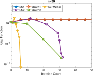
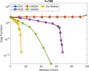
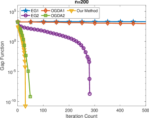
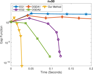
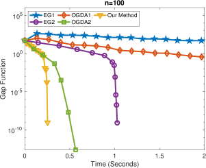
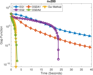
Figure 1: Performance of all the algorithms for $n\in\{50,100,200\}$ when $\rho=\frac{1}{20n}$ is set. The numerical results are presented in terms of iteration count (Top) and computational time (Bottom).

5.1 Cubic regularized bilinear min-max problem

Following the setup of Jiang and Mokhtari (2022), we consider the problem in the following form:

$$\min_{\mathbf{x}\in\mathbb{R}^{n}}\max_{\mathbf{y}\in\mathbb{R}^{n}}\ f(\mathbf{x},\mathbf{y})=\tfrac{\rho}{6}\|\mathbf{x}\|^{3}+\mathbf{y}^{\top}(A\mathbf{x}-\mathbf{b}),$$ (5.1)

where $\rho>0$, the entries of $\mathbf{b}\in\mathbb{R}^{n}$ are generated independently from $[-1,1]$ and $A\in\mathbb{R}^{n\times n}$ is given by

$$A=\begin{bmatrix}1&-1&&&\\ &1&-1&&\\ &&\ddots&\ddots&\\ &&&1&-1\\ &&&&1\end{bmatrix}.$$

This min-max optimization problem is convex-concave and the function $f$ is $\rho$-Hessian Lipschitz. It has a unique global saddle point $\mathbf{x}^{\star}=A^{-1}\mathbf{b}$ and $\mathbf{y}^{\star}=-\frac{\rho}{2}\|\mathbf{x}^{\star}\|(A^{\top})^{-1}\mathbf{x}^{\star}$. Then, we use the restricted gap function defined in Section 2 as the evaluation metric. In our experiment, the parameters are chosen as $\rho=\frac{1}{20n}$ and $n\in\{50,100,200\}$. Since the exact Hessian of $f$ is available here and the subproblem can be computed up to a high accuracy (using nonlinear equation solvers in MATLAB), we apply Algorithm 1. The baseline methods include EG1, OGDA1, EG2 (Bullins and Lai, 2022; Monteiro and Svaiter, 2012) and OGDA2 (Jiang and Mokhtari, 2022) where all of these methods require the exact Hessian. We implement EG2 using the pseudocode of Algorithm 5.2 and 5.3 in Bullins and Lai (2022) with fine-tuning parameters. The implementation of OGDA2 is based on the code from the author of Jiang and Mokhtari (2022) with $(\alpha,\beta)=(0.5,0.8)$. For a fair comparison, we solve the subproblems in second-order methods using same nonlinear system solvers in MATLAB.

In Figure 1, we compare our algorithm with five other baseline algorithms in terms of the gap function. Our results highlight that the second-order method can be far superior to the first-order method in terms of solution accuracy: the first-order method barely makes any progress when the second-order method converges successfully. Moreover, our method outperforms second-order methods (Bullins and Lai, 2022; Jiang and Mokhtari, 2022; Monteiro and Svaiter, 2012) in terms of both iteration numbers and computational time thanks to its simple scheme without line search. However, this does not eliminate the potential advantages of using line search in min-max optimization. Indeed, we observe that the line search scheme from Jiang and Mokhtari (2022) is powerful in practice and their algorithms with aggressive choices of $(\alpha,\beta)$ indeed outperform our method in some cases. However, such choices make their method unstable. Thus, we choose $(\alpha,\beta)=(0.5,0.8)$ which is conservative yet more robust. Nonetheless, we believe it is promising to study the line search scheme from Jiang and Mokhtari (2022) and see if modifications can speed up second-order min-max optimization in a universal manner.

5.2 AUC maximization problem

The problem of maximizing an area under the receiver operating characteristic curve (Hanley and McNeil, 1982) is a paradigm that learns a classifier for imbalanced data. It has a long history in machine learning (Graepel and Obermayer, 2000) and has motivated many studies ranging from formulations to algorithms and theory (Yang and Ying, 2022). The goal is to find a classifier $\theta\in\mathbb{R}^{n}$ that maximizes the AUC score on a set of samples $\{(\mathbf{a}_{i},b_{i})\}_{i=1}^{N}$, where $\mathbf{a}_{i}\in\mathbb{R}^{n}$ and $b_{i}\in\{-1,+1\}$.

Table 1: Statistics of datasets for AUC maximization.

Name	Description	$N$	$n$	Scaled Interval
a9a	UCI adult	48842	123	$\left[0,1\right]$
covetype	forest covetype	581012	54	$\left[0,1\right]$
w8a	-	64700	300	$[0,1]$

We can consider the min-max formulation for AUC maximization (Ying et al., 2016; Shen et al., 2018):

$$\min_{\mathbf{x}=(\theta,u,v)\in\mathbb{R}^{n+2}}\max_{y\in\mathbb{R}}\ \tfrac{1-\hat{p}}{N}\left\{\sum_{i=1}^{N}(\theta^{\top}\mathbf{a}_{i}-u)^{2}\mathbb{I}_{[b_{i}=1]}\right\}+\tfrac{\hat{p}}{N}\left\{\sum_{i=1}^{N}(\theta^{\top}\mathbf{a}_{i}-v)^{2}\mathbb{I}_{[b_{i}=-1]}\right\}$$

$$+\tfrac{2(1+y)}{N}\left\{\sum_{i=1}^{N}\theta^{\top}\mathbf{a}_{i}(\hat{p}\mathbb{I}_{[b_{i}=-1]}-(1-\hat{p})\mathbb{I}_{[b_{i}=1]})\right\}+\tfrac{\rho}{6}\|\mathbf{x}\|^{3}-\hat{p}(1-\hat{p})y^{2},$$

where $\lambda>0$ is a scalar, $\mathbb{I}_{[\cdot]}$ is an indicator function and $\hat{p}=\frac{\#\{i:b_{i}=1\}}{N}$ be the proportion of samples with positive label. It is clear that the min-max optimization problem in Eq. (5.2) is convex-concave and has the finite-sum structure in the form of Eq. (4.2) with the function $f_{i}(\mathbf{x},y)$ given by

$$f_{i}(\mathbf{x},y)=(1-\hat{p})(\theta^{\top}\mathbf{a}_{i}-u)^{2}\mathbb{I}_{[b_{i}=1]}+\hat{p}(\theta^{\top}\mathbf{a}_{i}-v)^{2}\mathbb{I}_{[b_{i}=-1]}$$

$$+2(1+y)\theta^{\top}\mathbf{a}_{i}(\hat{p}\mathbb{I}_{[b_{i}=-1]}-(1-\hat{p})\mathbb{I}_{[b_{i}=1]})+\tfrac{\rho}{6}\|\mathbf{x}\|^{3}-\hat{p}(1-\hat{p})y^{2}.$$

The above function is in the cubic form and the min-max problem has a global saddle point. We use the restricted gap function as the evaluation metric. In our experiment, the parameter is chosen empirically as $\rho=\frac{1}{N}$ and we use three LIBSVM datasets for AUC maximization (see Table 1). Since this min-max problem has a finite-sum structure, we can apply Algorithm 3 with uniform sampling. The baseline methods include Algorithm 2 as well as SEG and SOGDA (Juditsky et al., 2011; Hsieh et al., 2019; Mertikopoulos et al., 2019; Kotsalis et al., 2022). We choose the stepsizes for SEG and SOGDA in the form of $\frac{c}{\sqrt{k+1}}$ where $c>0$ is tuned using grid search and $k$ is the iteration count. For Algorithm 2, we choose $\kappa_{m}=0.1$. For Algorithm 3, we choose $\kappa_{m}=0.1$, $\delta=0.01$ and $|\mathcal{S}_{k}|=\frac{5\log(d+3)}{\min\{\|\nabla f(\hat{\mathbf{z}}_{k})\|^{2},\|\nabla f(\mathbf{z}_{k})\|^{2}\}}$. It is worth mentioning that $\min\{\|\nabla f(\hat{\mathbf{z}}_{k})\|^{2},\|\nabla f(\mathbf{z}_{k})\|^{2}\}$ is used instead of $\|\nabla f(\hat{\mathbf{z}}_{k})\|^{2}$ for practical purpose and such choice does not violate our theoretical setup. For the subproblem solving, we apply the semi-smooth Newton method as described before.

In Figure 2, we compare Algorithm 3 with Algorithm 2 and stochastic first-order methods. Our results show that Algorithm 3 outperforms SEG/SOGDA in terms of solution quality: SEG and SOGDA barely move when Algorithm 3 still makes significant progress. Compared to Algorithm 2, Algorithm 3 achieves similar solution quality eventually but require fewer samples to output an acceptable solution. It is also worth remarking that Algorithm 3 exhibits the (super)-linear convergence as the iterate approaches the optimal solution regardless of subsampling and inexact subproblem solving. This intriguing property has been rigorously justified for the subsampled Newton method in the context of convex optimization (Roosta-Khorasani and Mahoney, 2019), and it would be interesting to extend such results to min-max optimization.

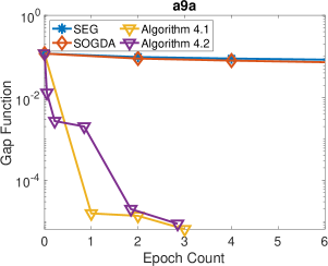
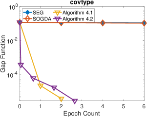
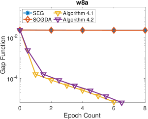
Figure 2: Performance of all the algorithms with 3 LIBSVM datasets when $\rho=\frac{1}{N}$ is set. The numerical results are presented in terms of epoch count (Top) and computational time (Bottom).

6 Conclusions

In this paper, we propose and analyze exact and inexact regularized Newton-type methods for finding a global saddle point of unconstrained and convex-concave min-max optimization problems with bounded and Lipschitz-continuous Hessian. We prove that our methods achieve an optimal convergence rate of $O(\epsilon^{-2/3})$. Moreover, we show that our framework and analysis on inexact algorithms lead to the first subsampled Newton method for solving the finite-sum min-max optimization problems with global convergence guarantee. Future research directions include the extension of our results to more general nonconvex-nonconcave min-max optimization problems and the customized implementation of our algorithms in real application problems.

References

• Abernethy et al. [2021] J. Abernethy, K. A. Lai, and A. Wibisono. Last-iterate convergence rates for min-max optimization: Convergence of Hamiltonian gradient descent and consensus optimization. In ALT, pages 3–47. PMLR, 2021.
• Adil et al. [2022] D. Adil, B. Bullins, A. Jambulapati, and S. Sachdeva. Optimal methods for higher-order smooth monotone variational inequalities. ArXiv Preprint: 2205.06167, 2022.
• Alizadeh and Goldfarb [2003] F. Alizadeh and D. Goldfarb. Second-order cone programming. Mathematical Programming, 95(1):3–51, 2003.
• Antipin [1978] A. S. Antipin. Method of convex programming using a symmetric modification of Lagrange function. Matekon, 14(2):23–38, 1978.
• Arjovsky et al. [2017] M. Arjovsky, S. Chintala, and L. Bottou. Wasserstein generative adversarial networks. In ICML, pages 214–223. PMLR, 2017.
• Beck and Teboulle [2009] A. Beck and M. Teboulle. A fast iterative shrinkage-thresholding algorithm for linear inverse problems. SIAM Journal on Imaging Sciences, 2(1):183–202, 2009.
• Ben-Tal et al. [2009] A. Ben-Tal, L. EL Ghaoui, and A. Nemirovski. Robust Optimization, volume 28. Princeton University Press, 2009.
• Berahas et al. [2020] A. S. Berahas, R. Bollapragada, and J. Nocedal. An investigation of Newton-sketch and subsampled Newton methods. Optimization Methods and Software, 35(4):661–680, 2020.
• Blackwell and Girshick [1979] D. A. Blackwell and M. A. Girshick. Theory of Games and Statistical Decisions. Courier Corporation, 1979.
• Bullins and Lai [2022] B. Bullins and K. A. Lai. Higher-order methods for convex-concave min-max optimization and monotone variational inequalities. SIAM Journal on Optimization, 32(3):2208–2229, 2022.
• Carmon et al. [2022] Y. Carmon, D. Hausler, A. Jambulapati, Y. Jin, and A. Sidford. Optimal and adaptive Monteiro-Svaiter acceleration. In NeurIPS, pages 20338–20350, 2022.
• Chambolle and Pock [2011] A. Chambolle and T. Pock. A first-order primal-dual algorithm for convex problems with applications to imaging. Journal of Mathematical Imaging and Vision, 40(1):120–145, 2011.
• Chen et al. [2022] X. Chen, B. Jiang, T. Lin, and S. Zhang. Accelerating adaptive cubic regularization of Newton’s method via random sampling. Journal of Machine Learning Research, 23(90):1–38, 2022.
• Chen et al. [2014] Y. Chen, G. Lan, and Y. Ouyang. Optimal primal-dual methods for a class of saddle point problems. SIAM Journal on Optimization, 24(4):1779–1814, 2014.
• Dantzig [1963] G. B. Dantzig. Linear Programming and Extensions. Princeton University Press, 1963.
• Daskalakis et al. [2018] C. Daskalakis, A. Ilyas, V. Syrgkanis, and H. Zeng. Training GANs with optimism. In ICLR, 2018. URL https://openreview.net/forum?id=SJJySbbAZ.
• Drineas and Mahoney [2018] P. Drineas and M. W. Mahoney. Lectures on randomized numerical linear algebra. The Mathematics of Data, 25(1), 2018.
• Facchinei and Pang [2007] F. Facchinei and J-S. Pang. Finite-Dimensional Variational Inequalities and Complementarity Problems. Springer Science & Business Media, 2007.
• Goodfellow et al. [2014] I. Goodfellow, J. Pouget-Abadie, M. Mirza, B. Xu, D. Warde-Farley, S. Ozair, A. Courville, and Y. Bengio. Generative adversarial nets. In NIPS, pages 2672–2680, 2014.
• Graepel and Obermayer [2000] T. Graepel and K. Obermayer. Large margin rank boundaries for ordinal regression. In Advances in Large Margin Classifiers, pages 115–132. The MIT Press, 2000.
• Gross and Nesme [2010] D. Gross and V. Nesme. Note on sampling without replacing from a finite collection of matrices. ArXiv Preprint: 1001.2738, 2010.
• Hanley and McNeil [1982] J. A. Hanley and B. J. McNeil. The meaning and use of the area under a receiver operating characteristic (ROC) curve. Radiology, 143(1):29–36, 1982.
• He and Monteiro [2016] Y. He and R. D. C. Monteiro. An accelerated HPE-type algorithm for a class of composite convex-concave saddle-point problems. SIAM Journal on Optimization, 26(1):29–56, 2016.
• Hsieh et al. [2019] Y-G. Hsieh, F. Iutzeler, J. Malick, and P. Mertikopoulos. On the convergence of single-call stochastic extra-gradient methods. In NeurIPS, pages 6938–6948, 2019.
• Huang et al. [2022] K. Huang, J. Zhang, and S. Zhang. Cubic regularized Newton method for the saddle point models: A global and local convergence analysis. Journal of Scientific Computing, 91(2):1–31, 2022.
• Jiang and Mokhtari [2022] R. Jiang and A. Mokhtari. Generalized optimistic methods for convex-concave saddle point problems. ArXiv Preprint: 2202.09674, 2022.
• Jiang et al. [2021] R. Jiang, M-C. Yue, and Z. Zhou. An accelerated first-order method with complexity analysis for solving cubic regularization subproblems. Computational Optimization and Applications, 79:471–506, 2021.
• Juditsky et al. [2011] A. Juditsky, A. Nemirovski, and C. Tauvel. Solving variational inequalities with stochastic mirror-prox algorithm. Stochastic Systems, 1(1):17–58, 2011.
• Kanzow et al. [2009] C. Kanzow, I. Ferenczi, and M. Fukushima. On the local convergence of semismooth Newton methods for linear and nonlinear second-order cone programs without strict complementarity. SIAM Journal on Optimization, 20(1):297–320, 2009.
• Kolossoski and Monteiro [2017] O. Kolossoski and R. D. C. Monteiro. An accelerated non-Euclidean hybrid proximal extragradient-type algorithm for convex-concave saddle-point problems. Optimization Methods and Software, 32(6):1244–1272, 2017.
• Korpelevich [1976] G. M. Korpelevich. The extragradient method for finding saddle points and other problems. Matecon, 12:747–756, 1976.
• Kotsalis et al. [2022] G. Kotsalis, G. Lan, and T. Li. Simple and optimal methods for stochastic variational inequalities, I: Operator extrapolation. SIAM Journal on Optimization, 32(3):2041–2073, 2022.
• Kovalev and Gasnikov [2022] D. Kovalev and A. Gasnikov. The first optimal acceleration of high-order methods in smooth convex optimization. In NeurIPS, pages 35339–35351, 2022.
• Lan [2020] G. Lan. First-Order and Stochastic Optimization Methods for Machine Learning, volume 1. Springer, 2020.
• Li et al. [2018a] X. Li, D. Sun, and K-C. Toh. A highly efficient semismooth Newton augmented Lagrangian method for solving Lasso problems. SIAM Journal on Optimization, 28(1):433–458, 2018a.
• Li et al. [2018b] Y. Li, Z. Wen, C. Yang, and Y-X. Yuan. A semismooth Newton method for semidefinite programs and its applications in electronic structure calculations. SIAM Journal on Scientific Computing, 40(6):A4131–A4157, 2018b.
• Liang and Stokes [2019] T. Liang and James Stokes. Interaction matters: A note on non-asymptotic local convergence of generative adversarial networks. In AISTATS, pages 907–915. PMLR, 2019.
• Lin and Jordan [2022] T. Lin and M. I. Jordan. Perseus: A simple and optimal high-order method for variational inequalities. ArXiv Preprint: 2205.03202, 2022.
• Lin and Jordan [2023] T. Lin and M. I. Jordan. Monotone inclusions, acceleration and closed-loop control. Mathematics of Operations Research, To appear, 2023.
• Lin et al. [2020] T. Lin, C. Jin, and M. I. Jordan. Near-optimal algorithms for minimax optimization. In COLT, pages 2738–2779. PMLR, 2020.
• Lobo et al. [1998] M. S. Lobo, L. Vandenberghe, S. Boyd, and H. Lebret. Applications of second-order cone programming. Linear Algebra and Its Applications, 284(1-3):193–228, 1998.
• Mertikopoulos et al. [2019] P. Mertikopoulos, B. Lecouat, H. Zenati, C-S. Foo, V. Chandrasekhar, and G. Piliouras. Optimistic mirror descent in saddle-point problems: Going the extra(-gradient) mile. In ICLR, 2019. URL https://openreview.net/forum?id=Bkg8jjC9KQ.
• Milzarek and Ulbrich [2014] A. Milzarek and M. Ulbrich. A semismooth Newton method with multidimensional filter globalization for $l_{1}$-optimization. SIAM Journal on Optimization, 24(1):298–333, 2014.
• Milzarek et al. [2019] A. Milzarek, X. Xiao, S. Cen, Z. Wen, and M. Ulbrich. A stochastic semismooth Newton method for nonsmooth nonconvex optimization. SIAM Journal on Optimization, 29(4):2916–2948, 2019.
• Mokhtari et al. [2020a] A. Mokhtari, A. Ozdaglar, and S. Pattathil. A unified analysis of extra-gradient and optimistic gradient methods for saddle point problems: Proximal point approach. In AISTATS, pages 1497–1507. PMLR, 2020a.
• Mokhtari et al. [2020b] A. Mokhtari, A. E. Ozdaglar, and S. Pattathil. Convergence rate of o(1/k) for optimistic gradient and extragradient methods in smooth convex-concave saddle point problems. SIAM Journal on Optimization, 30(4):3230–3251, 2020b.
• Monteiro and Svaiter [2010] R. D. C. Monteiro and B. F. Svaiter. On the complexity of the hybrid proximal extragradient method for the iterates and the ergodic mean. SIAM Journal on Optimization, 20(6):2755–2787, 2010.
• Monteiro and Svaiter [2011] R. D. C. Monteiro and B. F. Svaiter. Complexity of variants of Tseng’s modified FB splitting and Korpelevich’s methods for hemivariational inequalities with applications to saddle-point and convex optimization problems. SIAM Journal on Optimization, 21(4):1688–1720, 2011.
• Monteiro and Svaiter [2012] R. D. C. Monteiro and B. F. Svaiter. Iteration-complexity of a Newton proximal extragradient method for monotone variational inequalities and inclusion problems. SIAM Journal on Optimization, 22(3):914–935, 2012.
• Monteiro and Svaiter [2013] R. D. C. Monteiro and B. F. Svaiter. An accelerated hybrid proximal extragradient method for convex optimization and its implications to second-order methods. SIAM Journal on Optimization, 23(2):1092–1125, 2013.
• Nedić and Ozdaglar [2009] A. Nedić and A. Ozdaglar. Subgradient methods for saddle-point problems. Journal of Optimization Theory and Applications, 142(1):205–228, 2009.
• Nemirovski [2004] A. Nemirovski. Prox-method with rate of convergence o(1/t) for variational inequalities with Lipschitz continuous monotone operators and smooth convex-concave saddle point problems. SIAM Journal on Optimization, 15(1):229–251, 2004.
• Nemirovski and Yudin [1983] A. Nemirovski and D. Yudin. Problem Complexity and Method Efficiency in Optimization. Wiley, 1983.
• Nesterov [1983] Y. Nesterov. A method for unconstrained convex minimization problem with the rate of convergence o(1/k2). Dokl. Akad. Nauk. SSSR, 269(3):543–547, 1983.
• Nesterov [2005] Y. Nesterov. Smooth minimization of non-smooth functions. Mathematical Programming, 103(1):127–152, 2005.
• Nesterov [2006] Y. Nesterov. Cubic regularization of Newton’s method for convex problems with constraints. Technical report, Université catholique de Louvain, Center for Operations Research and Econometrics (CORE), 2006.
• Nesterov [2007] Y. Nesterov. Dual extrapolation and its applications to solving variational inequalities and related problems. Mathematical Programming, 109(2):319–344, 2007.
• Nesterov [2008] Y. Nesterov. Accelerating the cubic regularization of Newton’s method on convex problems. Mathematical Programming, 112(1):159–181, 2008.
• Nesterov and Polyak [2006] Y. Nesterov and B. T. Polyak. Cubic regularization of Newton method and its global performance. Mathematical Programming, 108(1):177–205, 2006.
• Neumann [1928] J. V. Neumann. Zur theorie der gesellschaftsspiele. Mathematische Annalen, 100(1):295–320, 1928.
• Nikaidô and Isoda [1955] H. Nikaidô and K. Isoda. Note on non-cooperative convex game. Pacific Journal of Mathematics, 5(5):807–815, 1955.
• Ouyang and Xu [2021] Y. Ouyang and Y. Xu. Lower complexity bounds of first-order methods for convex-concave bilinear saddle-point problems. Mathematical Programming, 185(1):1–35, 2021.
• Pilanci and Wainwright [2017] M. Pilanci and M. J. Wainwright. Newton sketch: A near linear-time optimization algorithm with linear-quadratic convergence. SIAM Journal on Optimization, 27(1):205–245, 2017.
• Popov [1980] L. D. Popov. A modification of the Arrow-Hurwicz method for search of saddle points. Mathematical notes of the Academy of Sciences of the USSR, 28(5):845–848, 1980.
• Qi and Sun [1993] L. Qi and J. Sun. A nonsmooth version of Newton’s method. Mathematical Programming, 58(1):353–367, 1993.
• Roosta-Khorasani and Mahoney [2019] F. Roosta-Khorasani and M. W. Mahoney. Sub-sampled Newton methods. Mathematical Programming, 174(1):293–326, 2019.
• Roosta-Khorasani et al. [2014] F. Roosta-Khorasani, K. Van Den Doel, and U. Ascher. Stochastic algorithms for inverse problems involving PDEs and many measurements. SIAM Journal on Scientific Computing, 36(5):S3–S22, 2014.
• Saad and Schultz [1986] Y. Saad and M. H. Schultz. GMRES: A generalized minimal residual algorithm for solving nonsymmetric linear systems. SIAM Journal on Scientific and Statistical Computing, 7(3):856–869, 1986.
• Shalev-Shwartz and Ben-David [2014] S. Shalev-Shwartz and S. Ben-David. Understanding Machine Learning: From Theory to Algorithms. Cambridge University Press, 2014.
• Shamma [2008] J. Shamma. Cooperative Control of Distributed Multi-agent Systems. John Wiley & Sons, 2008.
• Shen et al. [2018] Z. Shen, A. Mokhtari, T. Zhou, P. Zhao, and H. Qian. Towards more efficient stochastic decentralized learning: Faster convergence and sparse communication. In ICML, pages 4624–4633. PMLR, 2018.
• Sinha et al. [2018] A. Sinha, H. Namkoong, and J. Duchi. Certifiable distributional robustness with principled adversarial training. In ICLR, 2018. URL https://openreview.net/forum?id=Hk6kPgZA-.
• Sion [1958] M. Sion. On general minimax theorems. Pacific Journal of Mathematics, 8(1):171–176, 1958.
• Solodov and Svaiter [1998] M. V. Solodov and B. F. Svaiter. A globally convergent inexact Newton method for systems of monotone equations. In Reformulation: Nonsmooth, Piecewise Smooth, Semismooth and Smoothing Methods, pages 355–369. Springer, 1998.
• Solodov and Svaiter [1999] M. V. Solodov and B. F. Svaiter. A hybrid approximate extragradient-proximal point algorithm using the enlargement of a maximal monotone operator. Set-Valued Analysis, 7(4):323–345, 1999.
• Sra et al. [2012] S. Sra, S. Nowozin, and S. J. Wright. Optimization for Machine Learning. MIT Press, 2012.
• Tseng [1995] P. Tseng. On linear convergence of iterative methods for the variational inequality problem. Journal of Computational and Applied Mathematics, 60(1-2):237–252, 1995.
• Tseng [2000] P. Tseng. A modified forward-backward splitting method for maximal monotone mappings. SIAM Journal on Control and Optimization, 38(2):431–446, 2000.
• Tseng [2008] P. Tseng. On accelerated proximal gradient methods for convex-concave optimization. submitted to SIAM Journal on Optimization, 2:3, 2008.
• Von Neumann and Morgenstern [1953] J. Von Neumann and O. Morgenstern. Theory of Games and Economic Behavior. Princeton University Press, 1953.
• Xiao et al. [2018] X. Xiao, Y. Li, Z. Wen, and L. Zhang. A regularized semi-smooth Newton method with projection steps for composite convex programs. Journal of Scientific Computing, 76(1):364–389, 2018.
• Xu et al. [2016] P. Xu, J. Yang, F. Roosta-Khorasani, C. Ré, and M. W. Mahoney. Sub-sampled Newton methods with non-uniform sampling. In NIPS, pages 3008–3016, 2016.
• Xu et al. [2020] P. Xu, F. Roosta, and M. W. Mahoney. Newton-type methods for non-convex optimization under inexact Hessian information. Mathematical Programming, 184(1):35–70, 2020.
• Yang and Ying [2022] T. Yang and Y. Ying. AUC maximization in the era of big data and AI: A survey. ACM Computing Surveys (CSUR), 2022.
• Ying et al. [2016] Y. Ying, L. Wen, and S. Lyu. Stochastic online AUC maximization. In NIPS, pages 451–459, 2016.
• Zhao et al. [2010] X-Y. Zhao, D. Sun, and K-C. Toh. A Newton-CG augmented Lagrangian method for semidefinite programming. SIAM Journal on Optimization, 20(4):1737–1765, 2010.
• Zhou and Toh [2005] G. Zhou and K-C. Toh. Superlinear convergence of a Newton-type algorithm for monotone equations. Journal of Optimization Theory and Applications, 125(1):205–221, 2005.