A Stack-Free Traversal Algorithm for Left-Balanced k-d Trees

Abstract

We present an algorithm that allows for find-closest-point and kNN-style traversals of left-balanced k-d trees, without the need for either recursion or software-managed stacks; instead using only current and last previously traversed node to compute which node to traverse next.

1 Introduction

K-d trees (see Figure 1) are powerful, versatile, and widely used spatial data structures for storing, managing, and performing queries on k-dimensional data. One particularly interesting type of k-d trees are those that are left-balanced and complete: for those, storing the tree’s nodes in level order means that the entire tree topology—i.e., which are the parent, left, or right child of a given node—can be deduced from each node’s array index. This means that such trees require zero overhead for storing child pointers or similar explicit tree topology data, which makes them particularly useful for large data, and for devices where memory is precious (such as GPUs, FPGAs, etc). Throughout the rest of this paper we will omit the adjectives left-balanced and complete, and simply refer to ”k-d trees”; but always mean those that are both left-balanced and complete.

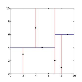
Figure 1: Illustration of a 2-dimensional k-d tree from Wikipedia [Wik]. Left: The balanced tree for 2D point set $\{(2,3),(5,4),(9,6),(4,7),(8,1),(7,2)\}$. Right: The space partitioning achieved by that tree.

One issue with k-d trees is that their hierarchical nature means that they work best with recursively formulated traversal techniques; but recursive formulations can be problematic on highly parallel architectures such as, for example, GPUs, FPGAs, dedicated hardware units, etc: true recursion—where functions can call themselves—is often hard or impossible to realize on such architectures, and is instead typically replaced with iterative algorithms that emulate recursion through a manually managed stack of not-yet-traversed sub-trees. Such “manual” stack based techniques do indeed avoid truly recursive function calls—and thus work just fine on GPUs—but can still cause several issues: for example, maintaining a stack per live thread (of which there will typically be many thousands) can require large amounts of temporary memory; it can lead to a significant amount of memory accesses (since such stacks are register-indirectly accessed they will typically end up in device memory); they can lead to hard-to-track errors if the reserved stack size isn’t large enough; etc.

In this paper, we describe a stack-free traversal algorithm for left-balanced k-d trees that does not require any stack at all, and instead only requires two integer values (for current and last traversed node IDs, respectively) to track all traversal state. In particular, our algorithm can handle both simple unordered traversals as well as the more channeling ordered kind where the traversal order of two children depends on which side of the parent’s partitioning plane the query point is located on. Our algorithm borrows from ideas we had previously developed for bounding volume hierarchies [HDWS11], and relies on using a state machine-like approach that, in each step, derives the respectively next node to be traversed from some relatively simple logic that only needs to know the current node that is currently traversed, and the one that was traversed in the previous step. We describe the core algorithm, provide some simple pseudo-code that realizes it, and present some performance data for a CUDA implementation of various variations of find-closest-point (fcp) and k-nearest-neighbor (kNN) queries that use this algorithm.

2 Related Work

k-d Trees (sometimes also referred to as kd-trees) are hierarchical spatial search trees used to encode k-dimensional data points [Sam90, Knu97, Wik]. Though the same term in graphics is also sometimes used to refer to a different kind of spatial subdivision tree (where inner code describe arbitrary partitioning planes and data are only stored in the leaves [WH06] ) for this paper we explicitly only consider the former kind, in which the data to be encoded are k-dimensional points, where points are stored also at inner nodes, and where partitioning planes are defined by the coordinates of the points stored at inner nodes (i.e., partitioning planes always pass through data points; see Figure 1).

Though k-d trees do not necessarily have to be balanced, one particularly interesting type of k-d trees are those that are left-balanced and complete, since these allow for storing the tree without any pointers or other explicit topology data. In graphics, these became famous through photon mapping [Jen01], in which k-d trees were used to memory-efficiently store—and efficiently perform k-nearest neighbor queries on—large numbers of photon. They have since become a method of choice for any kind of technique that requires storing and querying large numbers of point data.

This paper is about traversing such k-d trees, and in particular, in doing that in a stack-free manner. Mainly caused by the desired to finally achieve real-time ray tracing on graphics processing units (GPUs) the last decade has seen a concerted effort to develop such stack-free traversal techniques for ray traversal through bounding volume hierarchies (e.g., [Lai10, HDWS11, BAM13, ÁSK14, BK16, VWB19]). Such BVHes are different from k-d trees (and the queries we are targeting are different from ray traversal) but the motivation in both cases is the same: maintaining stacks can cause issues in highly parallel architectures where any per-thread state is potentially costly. In this paper, we primarily build on the technique described in [HDWS11], but adapt that to k-d trees and fcp/kNN-style traversals.

3 Algorithm

One issue with traversal algorithms for hierarchical data structures is that their requirements often come in many similar yet nevertheless slightly different forms; for example, whether the traversal need to be ordered vs un-ordered (i.e., whether the traversal order of two child nodes depends on the given query primitive or not); or whether the partitioning dimension of a k-d tree node is explicitly stored with the node vs implicitly fixed by the level of the node in the tree; or what exactly the traversal does with each visited data point (e.g., find-closest-point fcp vs k-nearest neighbors kNN); or whether the query primitive is a point/sphere (to find closest point or kNNs to) vs a box (to find all points within this box); etc.

In this section, we describe our algorithm for the following configuration:

• we assume an ordered traversal, where the traversal order for two children should always first traverse the child that is on the same side of the partitioning plane as the query point; a non-ordered traversal is a trivial simplification of this case.

• since ordered traversals are typically ordered relative to a single query point we assume a point as query primitive; replacing that with different query primitive types should be trivial.

• we assume that there is a shrinking max radius for the query, where the traversal can, while traversing, decide to exclude ever larger portions of the full tree based on whatever partial solution has already been found.

• we assume the tree is stored in the canonical way of using level-order (i.e., the root node is stored at array index 0, and the left and right child of a node $n$ are stored at $lChild(n)=2n+1$ and $rChild(n)=2n+2$).

• we make no assumptions about what partitioning plane dimension the builder chose for any given node; we simply assume existence of a function splitDimOf(node) that returns the partitioning dimension of this node.

3.1 Deriving the Traversal Logic

Using these assumptions, the core idea of our algorithm is to use a “state machine” like approach where we only track two integer values—the current node to be traversed, and the one that was traversed in the previous step—and use some simple observation to derive the next to-be-traversed node from that information. We observe that in a recursive formulation, the ordered traversal for any given sub-tree in a k-d tree looks like this:

1. process the current node (possibly shrinking the max query radius).

2. compute which of the two sub-trees is closer to the query point.

3. if close child exists: (recursively) traverse the sub-tree of the closer child.

4. if far child exists and sub-tree of far child still overlaps the current query range, recursively traverse that sub-tree.

For simplicity, let us re-formulate this as

1. if sub-tree is empty, return without doing anything.

2. process the current node (possibly shrinking the max query radius).

3. compute which of the two sub-trees is closer to the query point.

4. (recursively) traverse the sub-tree of the closer child.

5. if sub-tree of far child still overlaps the current query range, recursively traverse that sub-tree.

This is the exact same logic, except with the “if child exists” moved into the code for processing a given node.

If we now only look at any one particular node, and consider all the different cases that this recursive traversal would ever be “at” a given node, we can identify the following cases:

1. if the node in question does not exist, traversal will not do anything, and will simply go back to the parent node.

2. the first time a (valid) node gets traversed is when its traversal gets first called from its parent; in this case, it will first process the current node, and then go to the close child (which may or may not actually exist).

3. the second time a node gets visited is when recursion returns from the close child; in this case, there are two possible cases where the traversal will go next: if the far sub-tree is still in range, the next node to be traversed is the far child; otherwise, traversal is returning and the next node to traverse is the parent.

4. the third (and last) possible case where a node can gets visited is when recursion returns from the far child; in this case the next node to go to is the parent.

Using these rules, all we need to compute the next node to traverse is knowing which of these three cases we are in at any given point in time. The first case can be detected trivially by simply checking if the current node index is valid; the other three we can detect simply based on what the last traversed node was:

• the first-time-visit case only gets reached when the previous node was the parent, so if the previous node was the parent we process the current node and go to the close child.

• the second-time-visit case can only be reached if the previous node was the close child; in this case we need to test if the far sub-tree is in range, and next go to either far child or parent.

• the third-time-visit case can only be reached if the previous node was the far child; in this case we go to the parent (or terminate if we are at the root, obviously).

Using this formulation and applying this to every node that we are traversing will necessarily iterate through exactly the same nodes—in exactly the same order—as the recursive formulation we used above. All we need to do is keep track of both current and previous node ID, and apply this logic.

3.2 Pseudo-Code

In CUDA-like pseudo-code the algorithm can be expressed as follows:

⬇

void traverse(point queryPos, node *nodes, int N)

{

// current node: start at root

int curr = 0;

// previous node, initialize to "parent" of root node

int prev = -1;

float maxSearchRadius = ...;

// repeat until we break out:

while (true) {

int parent = (curr+1)/2-1;

if (curr >= N) {

// we reached a child that does not exist; go back to parent

prev = curr; curr = parent; continue;

}

bool from_parent = (prev < curr);

if (from_parent) {

processNode(curr);

// check if processing current node has led to

// a smaller search radius:

maxSearchRadius = possiblyShrunkenSearchRadius();

}

// compute close and far child:

int splitDim = splitDimOf(nodes,curr);

float splitPos = nodes[curr].coords[splitDim];

float signedDist = queryPoint[splitDim] - splitPos;

int closeSide = (signedDist > 0.f);

int closeChild = 2*curr+1+closeSide;

int farChild = 2*curr+2-closeSide;

bool farInRange = (fabsf(signedDist) <= maxSearchRadius);

// compute next node to step to

int next;

if (from_parent)

next = closeChild;

else if (prev == closeChild)

next = (farInRange ? farChild : parent);

else {

next = parent;

}

if (next == -1)

// the only way this can happen is if the entire tree under

// node number 0 (i.e., the entire tree) is done traversing,

// and the root node tries to step to its parent ... in

// which case we have traversed the entire tree and are done.

return;

// aaaand ... do the step

prev = curr; curr = next;

}

}

4 Evaluation

A sample implementation of this algorithm for various configurations of find-closest-point (fcp) and k-nearest-neighbors (kNN) can be found on github, at https://github.com/ingowald/cudaKDTree (see [Wal22a]). This repository also contains a gpu-based parallel k-d tree builder that is described in a related publication [Wal22b], but which this paper will not further comment upon other than observing that any tree built with this method will be the same exact left-balanced k-d tree that any other serial or CPU-based builder for such trees would produce, too.

Our sample traversal code is currently hard-coded for only two kernels: fcp, and knn for various $k$; but should be easy to adapted to other queries as well (in fact, it can easily be templated over a processNode() lambda). Similarly this code is hard-coded to float4 data types, but can trivially be adapted to (or templated over) other point types, including those with additional payload data (like, for example, surface normal and photon power for photon mapping), or to node types with an explicitly stored split dimension, etc.

To at least briefly evaluate this algorithm, we also added a very simple test rig that generates two arrays of uniformly distributed random float4 points in $[0,1]^{4}$, using a user-specified number of $N$ data points and a fixed $M=10,000,000$ query points; this test rig then then performs queries like fcp and kNN for various $k$ (including bounded and bounded variants for the kNN case). We run these on an NVIDIA RTX 3090TI card with 10,752 CUDA cores and 1.86 GHz boost clock, using Ubuntu 20.04.5 LTS, driver 510.85, and CUDA version 11.4; the results of these experiments are given in Table 1.

N	fcp	knn with k=… and maxR=$\inf$				knn with k=… and maxR=0.01
		k=4	k=8	k=20	k=50	k=4	k=8	k=20	k=50
1k	888M	563M	359M	48M	14M	5.2G	6.6G	4.0G	1.8G
10k	664M	407M	262M	29.5M	8.7M	3.3G	3.9G	3.3G	1.6G
100k	396M	184M	122M	20.6M	6.0M	1.7G	1.8G	1.7G	1.1G
1M	100M	42.1M	26.6M	7.5M	2.9M	334M	338M	282M	255M
10M	44M	19.3M	12.3M	5.0M	2.3M	58.2M	58.5M	52.8M	51M
100M	36M	16.5M	10.8M	4.7M	2.1M	19.1M	16.6M	14.2M	13.8M
200M	34.8M	16.2M	10.6M	4.5M	2.1M	16.7M	12.2M	9.2M	8.9M

Table 1: Results for our sample k-nearest neighbor (knn) and find-closest-point (fcp) use cases of our stack-free traversal algorithm, for various problem sizes and configurations. All order-of-magnitude indicators are multiples of 1000, not 1024, so “1M” means “1,000,000”. All results measured on an NVIDIA RTX 3090TI card, using the given number of (uniformly distributed) random input points in $[0,1]^{4}$, with 10M also uniform random distributed query points per kernel launch, and averaged over 100 such launches.

5 Summary and Conclusion

In this paper, we have described a stack-free k-d tree traversal algorithm that works on left-balanced k-d trees over k-dimensional points, and that can do both ordered and non-ordered traversal without requiring either recursion or manually managed stack; instead, all our algorithm requires as per-thread state are two ints to track the current and the respectively last previously traversed nodes, which our algorithm then uses to determine what to do in the current node, and where to go next. Our algorithm is both general and flexible, and on an RTX 3090TI and float4 data (with random uniform distributions) achieves traversal rates in the many millions of queries per second for both fcp and knn.

We make no claims that our sample implementation be the fastest possible implementation of this algorithm; nor even that this algorithm (even if it was implemented optimally) was guaranteed to be faster than a stack-based one; however, if and where a stack-free implementation is either required or desired we believe this algorithm to be a useful tool and viable solution.

Appendix A Revision History

Revision 1 (ArXiv version v2)

:

• Fixed two bugs in traversal pseudo-code that had crept in when simplifying the actual reference code into latex pseudo-code (original code and all measurements use correct code, only PDF had the bugs).

• Added cite and pointer to related parallel k-d tree construction paper

• Fixed missing URLs in References.

Original Version (ArXiv version v1)

: Originally uploaded to ArXiv Oct 23, 2022 https://arxiv.org/abs/2210.12859

References

- [ÁSK14] Attila T Áfra and László Szirmay-Kalos. Stackless Multi-BVH Traversal for CPU, MIC and GPU Ray Tracing. Computer Graphics Forum, 33(1):129–140, 2014.
- [BAM13] Rasmus Barringer and Tomas Akenine-Möller. Dynamic stackless binary tree traversal. Journal of Computer Graphics Techniques, 2(1):38–49, 2013.
- [BK16] Nikolaus Binder and Alexander Keller. Efficient stackless hierarchy traversal on GPUs with backtracking in constant time. In High Performance Graphics, pages 41–50, 2016.
- [HDWS11] Michal Hapala, Tomas Davidovic, Ingo Wald, and Philipp Slusallek. Efficient Stack-less BVH Traversal for Ray Tracing. In Proceedings of the 27th Spring Conference on Computer Graphics, 2011.
- [Jen01] Henrik Wann Jensen. Realistic image synthesis using photon mapping, volume 364. Ak Peters Natick, 2001.
- [Knu97] Donald Ervin Knuth. The art of computer programming, volume 3. Pearson Education, 1997.
- [Lai10] Samuli Laine. Restart trail for stackless BVH traversal. In Proceedings of the Conference on High Performance Graphics, pages 107–111. Citeseer, 2010.
- [Sam90] Hanan Samet. The design and analysis of spatial data structures, volume 85. Addison-wesley Reading, MA, 1990.
- [VWB19] Karthik Vaidyanathan, Sven Woop, and Carsten Benthin. Wide BVH traversal with a short stack. In Proceedings of the Conference on High-Performance Graphics, pages 15–19, 2019.
- [Wal22a] Ingo Wald. cudaKDTree: Sample code for GPU Construction and Stack-free Traversal of kd-Trees, 2022. https://github.com/ingowald/cudaKDTree.
- [Wal22b] Ingo Wald. GPU-friendly, Parallel, and (Almost-)In-Place Construction of Left-Balanced k-d Trees, 2022.
- [WH06] Ingo Wald and Vlastimil Havran. On building fast kd-Trees for Ray Tracing, and on doing that in O(N log N). In 2006 IEEE Symposium on Interactive Ray Tracing. IEEE, Sep 2006.
- [Wik] Wikipedia. k-d tree. https://en.wikipedia.org/wiki/K-d_tree, last visited Oct 23, 2022.