The Point-Boundary Art Gallery Problem is $\exists\mathbb{R}$-hard

Abstract

We resolve the complexity of the point-boundary variant of the art gallery problem, showing that it is $\exists\mathbb{R}$-complete, meaning that it is equivalent under polynomial time reductions to deciding whether a system of polynomial equations has a real solution.

Introduced by Victor Klee in 1973, the art gallery problem concerns finding configurations of guards which together can see every point inside of an art gallery shaped like a polygon. The original version of this problem has previously been shown to $\exists\mathbb{R}$-hard, but until now the complexity of the variant where guards only need to guard the walls of the art gallery was an open problem.

Our results can also be used to provide a simpler proof of the $\exists\mathbb{R}$-hardness of the point-point art gallery problem. In particular, we show how the algebraic constraints describing a polynomial system of equations can occur somewhat naturally in an art gallery setting.

1 Introduction

1.1 Art gallery problem

The original form of the art gallery problem presented by Victor Klee (see O’Rourke [12]) is as follows:

We say that a polygon $P$ (here containing its boundary) can be guarded by $n$ guards if there is a set of $n$ points (called the guards) in $P$ such that every point in $P$ is visible to some guard, that is the line segment between the point and guard is contained in the polygon. The problem asks, for a given polygon $P$ (which we refer to as the art gallery), to find the smallest $n$ such that $P$ can be guarded by $n$ guards.

The vertices of $P$ are usually restricted to rational or integral coordinates, but even so an optimal configuration might require guards with irrational coordinates (see Abrahamsen, Adamaszek and Miltzow [1] for specific examples of polygons where this is the case). For this reason, we don’t expect algorithms to actually output the guarding configurations, only to determine how many guards are necessary.

The art gallery problem (and any variant thereof) can be phrased as a decision problem: “can gallery $P$ be guarded with at most $k$ guards?” The complexity of this problem is the subject of this paper. Approximation algorithms can also be studied, see for example Bonnet and Miltzow [6].

1.2 The complexity class $\exists\mathbb{R}$

The decision problem ETR (Existential Theory of the Reals) asks whether a sentence of form:

$$\exists X_{1}\dots\exists X_{n}\Phi(X_{1},\dots,X_{n})$$

is true, where $\Phi$ is a formula $X_{i}$ involving $0$, $1$, $+$, $-$, $\cdot$, $=$, $<$, $\leq$, $\neg$, $\wedge$, and $\vee$. The complexity class $\exists\mathbb{R}$ consists of problems which can be reduced to ETR in polynomial time. A number of interesting problems have been shown to be complete for $\exists\mathbb{R}$, including for example the 2-dimensional packing problem [3] and the problem of deciding whether there exists a point configuration with a given order type [11][15].

By a result of Schaefer and Stefankovic [13], the exact inequalities used don’t matter; for example we obtain an equivalent definition of $\exists\mathbb{R}$ if we don’t allow $=$, $\leq$, or $\neg$ in $\Phi$. Recently, it is has been shown that some similar results hold at every level of the real hierarchy (of which $\exists\mathbb{R}$ is the first level) [14].

It is straightforward to show that $\text{NP}\subseteq\exists\mathbb{R}$, and it is also known, though considerably more difficult to prove, that $\exists\mathbb{R}\subseteq\text{PSPACE}$ (see Canny [7]). It is unknown whether either inclusion is strict.

1.3 Art gallery variants

There are several variants of this problem. We will be interested in ones involving restrictions on the placement of guards and of the region that must be guarded. We will adopt the notation used by Agrawal, Knudsen, Lokshtanov, Saurabh, and Zehavi in [4]:

Definition 1.1.

(Agrawal et al) The X-Y Art Gallery problem, where $X,Y\in\{\text{Vertex},\text{Point},\text{Boundary}\}$, asks whether the polygon $P$ can be guarded with $n$ guards, where if $X=\text{Vertex}$ the guards are restricted to lie on the vertices of the polygons, if $X=\text{Boundary}$ the guards are restricted to lie on the boundary of the polygon, if $X=\text{Point}$ then the guards can be anywhere inside the polygon, and the region which must be guarded is determined by $Y$ analogously.

Table 1 lists these variants and the known bounds on complexity.

Variant	Complexity Lower Bound	Complexity Upper Bound
Vertex-Y	NP	NP
X-Vertex	NP	NP
Point-Point	$\exists\mathbb{R}$	$\exists\mathbb{R}$
Boundary-Point	$\exists\mathbb{R}$	$\exists\mathbb{R}$
Point-Boundary	NP	$\exists\mathbb{R}$
Boundary-Boundary	NP	$\exists\mathbb{R}$

Table 1: Variants of the art gallery problem

If $X$ or $Y$ is Vertex, then the problem is easily seen to be in NP. Lee and Lin [9] showed that all of these variants are NP-hard (the result is stated for all the X-Point variants, but their constructions also work for the other variants. See also [8]). More recently, Abrahamsen, Adamaszek, and Miltzow [2] showed that the Point-Point and Boundary-Point variants are $\exists\mathbb{R}$ complete. It is straightforward to extend their proof of membership in $\exists\mathbb{R}$ to any of these variants, but the $\exists\mathbb{R}$-hardness question remained open for the BG and BB variants.

1.4 Our results

Our main result is that the Point-Boundary variant of the art gallery problem is, up to polynomial time reductions, as hard as deciding whether a system of polynomial equations has a real solution.

Theorem 1.2.

The Point-Boundary variant of the art gallery problem is $\exists\mathbb{R}$-complete.

While the complexity of the boundary-boundary variant is still unsolved, this is enough to give an interesting corollary:

Corollary 1.3.

For $X,Y\in\{\text{Vertex},\text{Point},\text{Boundary}\}$, the X-Y art gallery problem has the same complexity as the Y-X art gallery problem.

1.5 Overview of our techniques

For a given ETR-problem $\Phi$, we show how to construct an art gallery $P$ and number $g$ such that $P$ can be guarded (in the Point-Boundary sense) by $g$ guards if and only if $\Phi$ has a solution.

In Section 2, we show that a problem which we call $\text{ETR-INV}^{rev}$ is $\exists\mathbb{R}$-hard. This problem is only a slight adaptation of the $\exists\mathbb{R}$-hard problem ETR-INV from [2], and is $\exists\mathbb{R}$-hard for very similar reasons. This allows us to avoid introducing extra gadgets to flip the orientation of guard segments. This step is not strictly necessary by a result of Miltzow and Schmiermann [10], but it seems worth noting that hardness of the Point-Boundary variant doesn’t depend on this more powerful result.

In Section 3, we show how to construct an art gallery which encodes a given instance of $\text{ETR-INV}^{rev}$. This idea is very similar to the proof of the $\exists\mathbb{R}$-hardness of the Point-Point variant given by Abrahamsen et al in [2]. We use the positions of guards in the art gallery to encode variables, and develop a number of gadgets which constrain these positions in such a way as to represent arithmetic operations like addition and inversion.

We first show how to copy the positions of guards in order to allow a variable to appear in multiple constraints. A copy gadget for the Point-Boundary art-gallery problem was first described by Stade and Tucker-Foltz [16]. We give an overview of this idea, and show that all the required copy gadgets can be placed without interfering with each other. This is somewhat difficult since the graph of shared variables between different constraints is non-planar in general, but we are able to give a relatively nice geometric argument.

We then construct self-contained constraint gadgets which enforce a constraint like $x+y\leq z$, $x+y\geq z$, $xy\leq z$ or $xy\geq z$ on a fixed set of guard positions. We give general methods for constructing these types of gadgets with novel geometric proofs. In particular, we give an easy way of constructing the geometry for $xy\leq z$ and $xy\geq z$ without needing to solve quadratic equations. This is an improvement on [2], which required a computer search to construct an inversion gadget with rational coordinates.

In Section 4, we conclude by remarking on the apparent duality between the X-Y and Y-X variants of the problem, and consider the remaining Boundary-Boundary variant.

2 The problem $\text{ETR-INV}^{rev}$

The proof of Theorem 1.2 is by reduction of the problem $\text{ETR-INV}^{rev}$ to the BG variant of the art gallery problem.

Definition 2.1.

($\text{ETR-INV}^{rev}$) In the problem $\text{ETR-INV}^{rev}$, we are given a set of real variables $\{x_{1},\dots,x_{n}\}$ and a set of inequalities of the form:

$$x=1,\quad xy\geq 1,\quad x\left(\frac{5}{2}-y\right)\leq 1,\quad x+y\leq z,\quad x+y\geq z,$$

for $x,y,z\in\{x_{1},\dots,x_{n}\}$. The goal is to decide whether there is a assignment of the $x_{i}$ satisfying these inequalities with each $x_{i}\in[\frac{1}{2},2]$.

Abrahamsen et al [2] proved the $\exists\mathbb{R}$-hardness of the point-point and boundary-point variants using a similar problem called ETR-INV. It is nearly trivial to reduce ETR-INV $\text{ETR-INV}^{rev}$, the only problem being that we have an $x\left(\frac{5}{2}-y\right)\leq 1$ but would need a constraint of form $xy\leq 1$.

Definition 2.2.

(Abrahamsen, Adamaszek, Miltzow [2]) (ETR-INV) In the problem ETR-INV, we are given a set of real variables $\{x_{1},\dots,x_{n}\}$ and a set of equations of the form:

$$x=1,\quad xy=1,\quad x+y=z,$$

for $x,y,z\in\{x_{1},\dots,x_{n}\}$. The goal is to decide whether there is a solution to the system of equations with each $x_{i}\in[\frac{1}{2},2]$.

Theorem 2.3.

(Abrahamsen, Adamaszek, Miltzow [2]) The problem ETR-INV is $\exists\mathbb{R}$-complete.

Geometrically, the constraint $xy\leq 1$ seems to be difficult to construct in any variant of the art gallery problem, at least if the guards representing $x$ and $y$ are oriented in the same direction. The inversion gadget in [2] effectively computes $x\left(\frac{5}{2}-y\right)=1$ and uses other gadgets to reverse the second variable. This, however, is not strictly necessary, since the proof of the $\exists\mathbb{R}$-hardness of ETR-INV can be easily modified to show the same result for $\text{ETR-INV}^{rev}$.

2.1 $\exists\mathbb{R}$-hardness of $\text{ETR-INV}^{rev}$

Lemma 2.4.

The problem $\text{ETR-INV}^{rev}$ is $\exists\mathbb{R}$-hard.

Proof.

The proof of the $\exists\mathbb{R}$-hardness of ETR-INV in [2] has the interesting property that every time the inversion constraint is used, at least one of the input variables has possible values limited to an interval $[a,b]$ of length less than $\frac{1}{2}$. If $x$ is such a variable, then it is possible with the addition constraints to create an auxiliary variable $V$ satisfying $V=\frac{5}{2}-x$. This allows the full inversion constraint to be constructed. The construction of $V$ follows.

Miltzow and Schmiermann [10] show that the addition and constant constraints are sufficient to construct a variable equal to any rational number (in $[\frac{1}{2},2]$), so by adding or subtracting constants, we can assume without loss of generality that $x\in[1,\frac{3}{2}]$. We can now construct the variable $V$:

$$V_{1}+V_{1}=x\quad\left(V_{1}=\frac{1}{2}x\in[\frac{1}{2},\frac{3}{4}]\right)$$

$$V_{1}+V_{2}=\frac{5}{4}\quad\left(V_{2}=\frac{5}{4}-\frac{1}{2}x\in[\frac{1}{2},\frac{3}{4}]\right)$$

$$V=V_{2}+V_{2}\quad\left(V=\frac{5}{2}-x\in[1,\frac{3}{2}]\right)$$

So the proof of the hardness of ETR-INV in [2] can be adapted to show that $\text{ETR-INV}^{rev}$ is $\exists\mathbb{R}$.

∎

Since the publication of [2], Miltzow and Schmiermann [10] have shown that, subject to some minor technical conditions, a continuous constraint satisfaction problem with an addition constraint, a convex constraint, and a concave constraint is $\exists\mathbb{R}$. This could be used to easily show that $\text{ETR-INV}^{rev}$ is $\exists\mathbb{R}$-hard. The advantage of our approach is that the reduction from ETR to $\text{ETR-INV}^{rev}$ is purely algebraic modulo the fact that ETR on bounded domains is $\exists\mathbb{R}$-hard [13].

3 Reduction from $\text{ETR-INV}^{rev}$ to the Point-Boundary art gallery problem

We are given an instance $\Phi$ of $\text{ETR-INV}^{rev}$ with $n$ variables. The goal is to construct an art gallery $P$ and integer $g$ such that $P$ can be guarded with $g$ guards if and only if $\Phi$ has a solution. First, we will show how to construct an art gallery where any guarding configuration with $g$ guards must have those guards in specific regions. We can extract the values of the variables from $\Phi$ from the coordinates of some of those guards. Next, we show how to impose constraints on pairs of guard positions so that multiple guards in different parts of the art gallery represent the value of the same variable in $\Phi$. Finally, we will show how to impose constraints corresponding to addition and inversion.

3.1 Notation

Here $AB$ refers to a line segment, $\overleftrightarrow{AB}$ is the line containing that segment, and $|AB|$ is the length of that segment.

3.2 Wedges and variable gadgets

We want the positions of certain guards to encode the values of variables in an instance of $\text{ETR-INV}^{rev}$. In order to do this, we need to know which guard corresponds to which variable. The idea is to designate $n$ disjoint guard regions inside the art gallery and show that any guarding configuration with exactly $n$ guards must have exactly one guard in each region. Each guard region is formed by some number of wedges.

Definition 3.1.

(Wedge) A wedge is formed by a pair of adjacent line segments on the boundary of the art gallery with an internal angle between them less than $\pi$. The visibility region of a wedge is the set of points which are visible to the tip of the wedge.

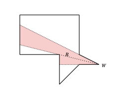
Figure 1: A wedge ($W$) and its visibility region ($R$)

Clearly, in a guarding configuration, the visibility region of each wedge must contain a guard, but if two visibility regions intersect then a single guard is sufficient to guard both wedges. In order for each guard region to necessarily contain a guard, we need to choose these wedges carefully.

Definition 3.2.

(Guard regions and guard segments) We will designate certain regions inside the art gallery called guard regions, which are each formed by the intersection of the visibility regions of some (non-zero) number of wedges. The visibility regions of wedges corresponding to different guard regions must not intersect. A guard region shaped like a line segment is called a guard segment.

Figure 2: The intersection of the visibility regions of the three wedges shown forms a guard segment. This method of using $3$ wedges to form a guard segment is due to Bertschinger et al [5] and is a slight simplification of the method for forming guard segments from [2].

Lemma 3.3.

If we designate $n$ guard regions, then any guarding configuration has at least $n$ guards, and a guarding configuration with exactly $n$ guards has $1$ guard in each guard region.

Proof.

Choose wedges $w_{1},\dots,w_{n}$, one from each of the guard regions. By assumption, the visibility regions of these wedges do not intersect. In a guarding configuration, each of these regions contains at least $1$ guard, so any such configuration contains at least $n$ guards.

If a guarding configuration contains exactly $n$ guards, then there will be exactly $1$ guard in each of these visibility regions. Now, suppose, the $i$th guard region is the intersection of the visibility regions of wedges $w_{i},v_{1},\dots v_{k}$. Each of the visibility regions of $v_{1},\dots,v_{k}$ must contain a guard, and since they do not intersect the visibility regions of $w_{j}$ for $j\neq i$, the guard in the visibility region of $w_{i}$ must also be in these regions, so is in the $i$th guard region. ∎

Having one guard in each guard region is a necessary but not sufficient condition for a configuration to be a guarding configuration. The gallery we construct will have some number of guard regions, with additional constraints on the positions of the guards which can be satisfied if and only if a given $\text{ETR-INV}^{rev}$ problem has a solution.

3.3 Nooks and continuous constraints

Continuous constraints between guards will be enforced by constraint nooks.

Definition 3.4.

(Nook) a nook consists of a line segment on the boundary of the art gallery, called the nook segment, and geometry around it to restrict the visibility of that segment. The region of partial visibility of a nook is the set of points which can see some part of the nook segment.

These differ from the nooks used by Abrahamsen et al in [2] in two ways. First, we will sometimes need intersect a convex vertex with a nook in order to help form a guard region, as in Figure 3. Second, we don’t require guard regions constrained by the nook to line up with the partial visibility region in any particular way.

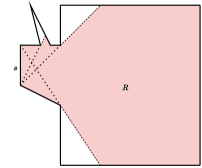
Figure 3: A nook with nook segment $s$ and partial visibility region $R$.

A guarding configuration will have some non-zero number of guards in the partial visibility region of a nook, which together must guard the nook segment, as in Figure 4. In general, no guard needs to see all of the nook segment, instead it can be guarded by a collaboration of several guards. The possible positions of one guard can then depend continuously on the position of another. In our construction, the partial visibility region of each constraint nook will intersect exactly $2$ guard regions. In order to create the addition constraints, we will need to use that fact that guards have $2$ coordinates, and so in some sense each nook enforces a constraint on up to $4$ variables.

Figure 4: This art gallery can be guarded by two guards, but there is no such configuration where the nook segment on the left is guarded entirely by a single guard. The possible positions of each guard depend continuously on the position of the other guard.

3.4 Art gallery setup

The art gallery we will construct will have two rows of guard segments. The variable segments in the middle left represent the variables $x_{1},\dots,x_{n}$. The input segments are at the bottom right. The $y$-coordinate of each of these guards represents the value of a variable in $[\frac{1}{2},2]$, with larger $y$-coordinates corresponding to larger values of the variable. Any other guard regions are referred to as auxiliary. Each constraint gadget constrains the positions of a set of $2$ or $3$ of the input segments relative to each other. In order to constrain the values of the original variables, each input segment to one of the variable segments by copy nook. Figure 5 shows an example of such an art gallery with $3$ variable segments (corresponding to variables $x$, $y$, and $z$) and gadgets enforcing constraints $x+z\geq y$ and $xy\geq 1$.

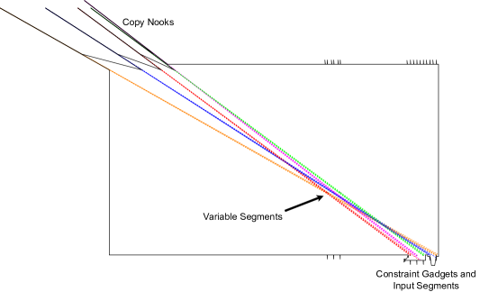
Figure 5: An art gallery with $3$ variable segments, $5$ input segments, and $2$ constraint gadgets. The variable and input segments are too small to see in this figure.

Figure 6: Detail of Figure 5 showing the variable segments, input segments, and constraint gadgets.

3.5 Copying

The copying construction used by Abrahamsen et al in [2] has an orientation dependence which means that, for a given pair of segments, a copy nook can only enforce one constraint out of $x\geq y$ or $x\leq y$. They obtain the other constraint in a way that relies on the need to guard the interior of the art gallery, so this won’t work in Point-Boundary setting. For this reason, we use a different geometric principle for our copy gadgets. This type of copy gadget was first described by Stade and Tucker-Foltz [16].

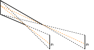
Figure 7: A copy nook. The two guards $g_{1}$ and $g_{2}$ guard the nook as long as $g_{2}$ is at or above the vertical position of $g_{1}$.

The nook segment is parallel to the two guard segments being copied, so the constraint enforced by this nook can be obtained by properties of similar triangles.

Lemma 3.5.

Suppose segments $AB$ and $CD$ are such that $\overleftrightarrow{AB}$ and $\overleftrightarrow{CD}$ are parallel, and suppose $\overleftrightarrow{AC}$ and $\overleftrightarrow{BD}$ intersect at a point $P$, as in Figure 8. If a line through $P$ intersects $AB$ at a point $X$ and intersects $CD$ at a point $Y$, then $\frac{|AX|}{|AB|}=\frac{|CY|}{|CD|}$.

Proof.

Triangles $APB$ and $CPD$ are similar, so $\frac{|AP|}{|AB|}=\frac{|CP|}{|CD|}$. Also, the triangles $AXP$ and $CYP$ are similar, so $\frac{|AX|}{|AP|}=\frac{|CY|}{|CP|}$. Multiplying, we obtain $\frac{|AX|}{|AB|}=\frac{|CY|}{|CD|}$. ∎

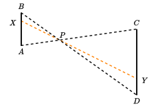
Figure 8: By Lemma 3.5, we have $\frac{|AX|}{|AB|}=\frac{|CY|}{|CD|}$.

Enforcing a constraint $x=y$ requires $2$ of these nooks, but all of the constraints in $\text{ETR-INV}^{rev}$ are monotone with respect to any single variable, so we only need a single copy nook for each input segment. For example, $xy\geq 1$ is equivalent to $x^{\prime}y^{\prime}\geq 1$, $x\geq x^{\prime}$ and $y\geq y^{\prime}$ as long as there are no other constraints on $x^{\prime}$ and $y^{\prime}$.

3.5.1 Specification of the copy nooks

This section is concerned with showing that it is indeed possible to arrange all the copy nooks in such a way that none of them interfere with each other. Additionally, we want some bound on the geometry of the copy nooks in order to make sure they don’t interfere with the constraint gadgets. In this section, we will assume we need $n$ variable segments and $i$ input segments. All the segments have length $1$, and both sets of segments occur at regular intervals with spacing $d$ in two horizontally aligned rows, which are separated by a vertical distance $h$. Let $A_{k}$ be the bottom of the $k$th input segment and let $B_{k}$ be top of this segment, and let $C_{j}D_{j}$ be the segment at the $j$th position in the row of input segments, as in Figure 9.

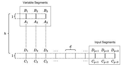
Figure 9: The variable and input segments. The first input segment should be to the right of the last variable segment.

For given variable and input segments, there are two types of nook which we might need to construct. If the guard on the variable segment represents a value $y$ and the guard on the input segment represents a variable $x$, then a $\geq$ copy nook (shown in Figure 10) enforces the constraint $x\geq y$, and a $\leq$ copy nook (Figure 11) enforces the constraint $x\leq y$.

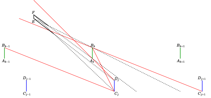
Figure 10:

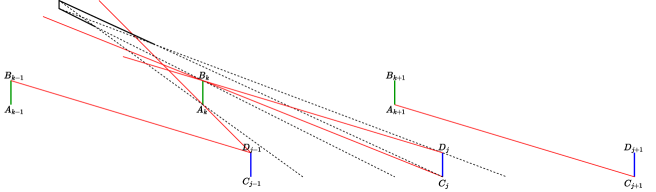
Figure 11:

Lemma 3.6 tells us how to construct a single one of either of these nooks.

Lemma 3.6.

Suppose for some $k$ and $j$ we have that $\overleftrightarrow{B_{k}C_{j+1}}$ doesn’t intersect $A_{k+1}B_{k+1}$. Then if the nook segment $EF$ for a $\geq$ copy nook between variable segment $v_{k}$ and input segment $s_{j}$ is placed above the line $\overleftrightarrow{B_{k}C_{j+1}}$ and below the line $\overleftrightarrow{A_{k}D_{j}}$ then no obstructions occur. That is, $\overleftrightarrow{EB_{k}}$ doesn’t intersect $v_{k+1}$ or $s_{j+1}$, $\overleftrightarrow{FC_{j}}$ doesn’t intersect $v_{k-1}$ or $s_{j-1}$, and $\overleftrightarrow{FA_{k}}$ doesn’t intersect $ED_{j}$. Furthermore, any line between the nook segment and either guard segment is steeper than $\overleftrightarrow{B_{k}C_{j+1}}$ and less steep than $\overleftrightarrow{B_{k}C_{j}}$.

Similarly, if $\overleftrightarrow{B_{k}D_{j}}$ doesn’t intersect $A_{k+1}B_{k+1}$ then a $\leq$ copy nook between variable segment $v_{k}$ and input segment $s_{j}$ will have no obstructions if the nook segment $EF$ is above the line $\overleftrightarrow{B_{k}C_{j}}$ and below the line $\overleftrightarrow{A_{k}D_{j-1}}$, and the lines between the nook segment and its guard segments have slope bounded by $\overleftrightarrow{B_{k}C_{j}}$ and $\overleftrightarrow{A_{k}D_{j-1}}$.

Proof.

See Figures 10 and 11. For the $\geq$ nook, it is the case that $\overleftrightarrow{FC_{j}}$ doesn’t intersect $A_{k-1}B_{k-1}$ since $\overleftrightarrow{FC_{j}}$ is steeper than $\overleftrightarrow{B_{k}C_{j+1}}$ and the lines $\overleftrightarrow{B_{k}C_{j+1}}$ and $\overleftrightarrow{B_{k-1}C_{j}}$ are parallel. The $\leq$ case is similar. ∎

For the purposes of constructing the constraint gadgets, we want the slopes of any line between a copy nook segment and one of its guard segments to have slope between $-\frac{1}{2}$ and $-1$. By Lemma 3.6, this will be true for a $\leq$ or $\geq$ nook between segments $A_{k}B_{k}$ and $C_{j}D_{j}$ as long as lines $\overleftrightarrow{B_{k}C_{j}}$, $\overleftrightarrow{B_{k}C_{j+1}}$, $\overleftrightarrow{A_{k}D_{j-1}}$, and $\overleftrightarrow{A_{k}D_{j}}$ have slopes in this range.

For general $k$ and $j$, the line $\overleftrightarrow{B_{k}C_{j}}$ has slope $-\frac{h+1}{d(j-k)}$ and the line $\overleftrightarrow{A_{k}D_{j}}$ has slope $-\frac{h-1}{d(j-k)}$. These are between $-\frac{1}{2}$ and $-1$ so long as:

$$\frac{1}{2}d(j-k)+1\leq h\leq d(j-k)-1$$ (1)

There $n$ variable segments and $i$ input segments, giving $n+i-1$ values of $j-k$. However, we also need these bounds to hold for one value of $j$ beyond the row of input segments in either direction, so we should choose $h$ so that the largest and smallest values of $j-k$ which satisfy (1) differ by at least $n+i+1$. These values of $j-k$ are

$$\frac{h+1}{d}\leq j-k\leq 2\frac{h-1}{d}$$

so as long as $d\geq 1$, it is sufficient to have $h\geq(n+i+2)d$.

If $d>2$, these conditions on the slopes of $\overleftrightarrow{B_{k}C_{j}}$ and $\overleftrightarrow{A_{k}D_{j}}$ also ensure that $\overleftrightarrow{B_{k}C_{j+1}}$ and $\overleftrightarrow{B_{k}D_{j}}$ don’t intersect $A_{k+1}B_{k+1}$ for these values of $j-k$.

This tells us how to construct nooks each of which only sees the correct pair of segments, but not how to construct all the nooks without them interfering with each other. The partial visibility regions of multiple nooks can intersect without issue, but the nook segment and the two walls of a nook must not occlude the partial visibility region of any other nook. Lemmas 3.7 and 3.8 will help us complete the construction.

Lemma 3.7.

If a $\leq$ or $\geq$ copy nook between $A_{k}B_{k}$ and $C_{j}D_{j}$ has nook segment $EF$ with length $\alpha$ and the horizontal distance between the nook segment and $\overleftrightarrow{C_{j}D_{j}}$ is $\beta$, then all the walls of the nook are a horizontal distance at least $\beta\frac{1}{1+\alpha}$ from $\overleftrightarrow{C_{j}D_{j}}$, as in Figure 12. In particular this distance can be made arbitrarily large by increasing $\beta$.

Proof.

Calculate the intersection point of $\overleftrightarrow{ED_{j}}$ and $\overleftrightarrow{FC_{j}}$ (see Figure 12). ∎

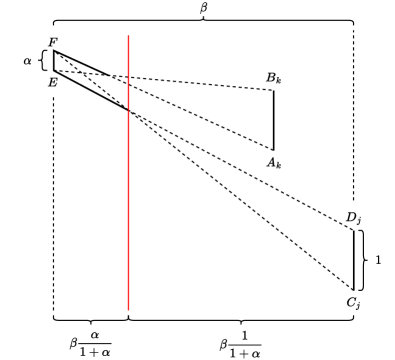
Figure 12: Illustration of Lemma 3.7

.

Lemma 3.8.

Suppose lines $\ell_{1}$ starting at $B_{k}$ and $\ell_{2}$ starting at $D_{j}$ are parallel, as in Figure 3.8. Then if a $\leq$ or $\geq$ nook between segments $A_{k}B_{k}$ and $C_{j}D_{j}$ has a nook segment which is in the tubular region bounded by $\ell_{1}$ and $\ell_{2}$, then all points in the partial visibility region of the nook which are to the left of $\overleftrightarrow{A_{k}B_{k}}$ are inside the same tubular region.

Proof.

See Figure 13. ∎

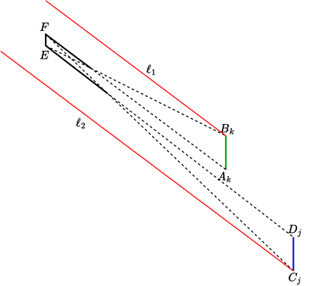
Figure 13: Illustration of Lemma 3.8

We can now construct all the copy nooks.

Lemma 3.9.

Suppose there is some $p$ such that for any $1\leq k\leq n$ and $p\leq j\leq p+i$ we have that $\overleftrightarrow{A_{k}D_{j}}$ is steeper than $\overleftrightarrow{B_{k}C_{j+1}}$ by a slope of more than $\epsilon$, and these lines meet the conditions from Lemma 3.6. Then we can construct any number of non-interfering $\geq$ or $\leq$ copy nooks between variable segments $A_{k}B_{k}$ and input segments $C_{j}D_{j}$ for $1\leq k\leq n$ and $p+1\leq j\leq p+i$.

Proof.

For a copy nook between $A_{k}B_{k}$ and $C_{j}D_{j}$, we want to create a tube in order to apply Lemma 3.8. We should to be able to place a nook segment arbitrarily far along the tube without violating the assumptions of Lemma 3.6. For a $\geq$ nook, the lines $\ell_{1}$ and $\ell_{2}$ should have slope steeper than $\overleftrightarrow{A_{k}D_{j}}$ and less steep than $\overleftrightarrow{B_{k}C_{j+1}}$, as in Figure 14. For a $\leq$ nook, we instead bound by lines $\overleftrightarrow{A_{k}D_{j-1}}$ and $\overleftrightarrow{B_{k}C_{j}}$. By the conditions of the slopes of $\overleftrightarrow{A_{k}D_{j}}$ and $\overleftrightarrow{B_{k}C_{j+1}}$, we can choose always choose this tube so that the slope is an integer multiple of $\frac{1}{2}\epsilon$.

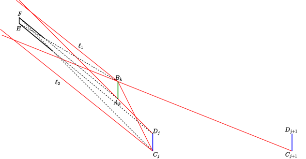
Figure 14: A tube for Lemma 3.8 which is contained in the region from Lemma 3.6 for points sufficient far to the left.

Since $\overleftrightarrow{A_{k}D_{j}}$ is stepper than $\overleftrightarrow{A_{k}D_{j+1}}$, the only way for two parallel tubes chosen this way to intersect is if there is a $\geq$ copy nook between $A_{k}B_{k}$ and $C_{j}D_{j}$ and a $\leq$ copy nook between $A_{k}B_{k}$ and $C_{j+1}D_{j+1}$. If this happens, then the regions for placing these nook segments coincide, but we choose the two tubes for these nooks to have different slopes.

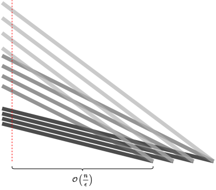
Figure 15: With the tubes chosen, we can place the copy nooks.

We can now choose a vertical line $v$ such that no point left of $v$ is in more than one tube, as in Figure 15. The horizontal distance from $A_{1}B_{1}$ to $v$ is at most $\mathcal{O}(n\epsilon^{-1})$. Using Lemma 3.7, we can construct a nook in each tube such that the walls of the nook are on the left of $v$, so by Lemma 3.8, none of these nooks interfere with each other, as required.

∎

What remains to show is that for any $n$ and $i$ we can choose $h$ and $d$ so that there exists a $p$ which satisfies the conditions of Lemma 3.9. The difference in slopes between $\overleftrightarrow{A_{k}D_{j}}$ and $\overleftrightarrow{B_{k}C_{j+1}}$ is:

$$\frac{h-1}{d(j-k)}-\frac{h+1}{d(j+1-k)}=\frac{h-1-2(j-k)}{d(j-k)(j+1-k)}$$

So we need $h>2(j-k)+2$, so that this is larger than $\epsilon=(d(j-k)(j+1-k))^{-1}$. Since $j-k$ will always be at least $1$, we can choose $d>8$, making this a strictly weaker condition than (1). So we should choose $h\geq(n+i+2)d$ and $d>8$. Since the value of $d$ doesn’t need to depend on $n$ or $i$, we will fix $d=9$ from here on.

3.6 Constraint gadgets

Next, we need to create the constraint gadgets which will actually enforce the constraints. Each constraint gadget will contain some number of nooks in order to enforce constraints on its input segments. The addition gadgets will each contain an extra guard region. It is important to position these nooks and auxiliary guard regions in such a way that they don’t interfere with the copy gadgets. The copy gadgets have been specified in such a way that this can be done independently of the exact details of the copy gadgets, as shown in Figure 16.

Figure 16: Diagram of a constraint gadget. The region $R_{1}$ is bounded by lines with slope $-1$ and $-\frac{1}{2}$. The region $R_{2}$ is bounded by lines with slope $-1$.

Each input segment is the intersection of the visibility region of three wedges; two will be on the top wall of the art gallery, but one must be on the bottom of the gadget. The distance from the constraint gadgets to the top wall depends on the number of variables and constraints, so the angle of each of these wedges also needs to depend on these numbers. Other than this, the geometry of each constraint gadget is fixed.

As long as the walls of the art gallery do not obstruct the region $R_{1}$, there can no obstruction to the visibility between the input segments and their copy nooks. Guards on the variable segments will never see anything outside the region $R_{2}$, so any constraint nooks should have nook segments which do not intersect this area. Also, the guard regions for any auxiliary guards used should avoid intersecting $R_{2}$ so that they don’t interfere with the copy gadgets. The visibility regions of wedges for each auxiliary guard region must also avoid intersecting the visibility regions of wedges for other guard regions. The auxiliary guard region (yellow) and nooks in Figure 16 satisfy these restrictions.

Each constraint gadget will have some number (either $2$ or $3$) of input guard segments, but might also take up additional spaces in the row of input segments. These spaces will be left empty.

Constraints of the form $x=1$ will not have a dedicated constraint gadget. Instead, these can be created by adding a wedge to a guard segment to turn it into a guard point, as in Figure 17.

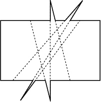
Figure 17: A point-shaped guard region.

The remaining constraints each need a constraint gadget. These constraints are:

$$xy\geq 1,\quad x\left(\frac{5}{2}-y\right)\leq 1,\quad x+y\leq z,\quad x+y\geq z$$

3.7 Inversion

The first gadgets we will create are the $xy\geq 1$ and $x\left(\frac{5}{2}-y\right)\leq 1$ gadgets. Figures 18 and 19 show the complete gadgets.

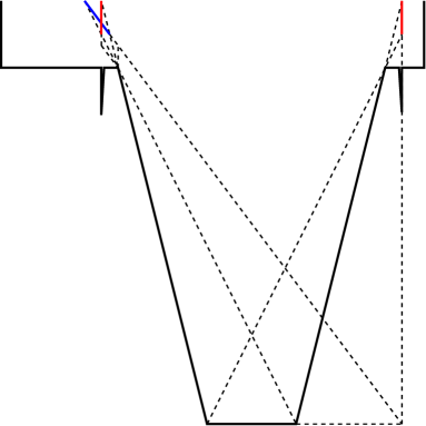
Figure 18: The $xy\geq 1$ gadget. The red segments are the guard segments. The constraint nook needs to be deep in order to avoid possible interference with the copy gadgets.

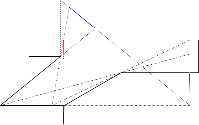
Figure 19: The $x\left(\frac{5}{2}-y\right)\leq 1$ gadget. The guard segment on the left represents the variable $x$.

It is straightforward to see that the constraint enforced by a nook between two guard segments is always of the form:

$$x\leq\frac{ay+b}{cy+d}$$

for some rational constants $a,b,c,d$. For a suitable linear change of bases $x^{\prime}=qx+p$, $y^{\prime}=ry+s$, this is equivalent to a constraint like:

$$x\leq y\text{ or }x\geq\frac{1}{y}\text{ or }x\leq\frac{1}{y}$$

The copy gadgets make use of linear constraints of form $x\leq y$. In order to construct both inversion gadgets, we need to show that both convex ($x\geq\frac{1}{y}$) and concave ($x\leq\frac{1}{y}$) constraints can occur. Lemmas 3.10 and 3.11 will be used to show that this is the case, and will allow us to construct the exact inversion constraints that we want.

Lemma 3.10.

Given non-parallel line segments $AB$ and $CD$, as in Figure 20, say that $\overleftrightarrow{AD}$ and $\overleftrightarrow{BC}$ intersect at a point $P$. Let $E$ be the point on $\overleftrightarrow{AB}$ such that $\overleftrightarrow{PE}$ and $\overleftrightarrow{CD}$ are parallel, and let $F$ be the point on $\overleftrightarrow{CD}$ such that $\overleftrightarrow{PF}$ and $\overleftrightarrow{AB}$ are parallel. Draw a line through $P$ intersecting $AB$ at $X$ and $CD$ at $Y$. Then $\frac{|EA|}{|EB|}=\frac{|FC|}{|FD|}$, and letting $\alpha^{2}=|EA||EB|$ and $\beta^{2}=|FC||FD|$ we have $\frac{|EX|}{\alpha}\cdot\frac{|FY|}{\beta}=1$.

Since we want to enforce inversion constraints on variables in the range $[\frac{1}{2},2]$, we will use geometry so that $|EB|=4|EA|$ (and therefore $|FD|=4|FC|$), so $\alpha=2|EA|=\frac{1}{2}|EB|$ and $\beta=2|FC|=\frac{1}{2}|FD|$. This means that $\frac{|EX|}{\alpha}$ and $\frac{|FY|}{\beta}$ will map the segments $AB$ and $CD$ respectively onto $[\frac{1}{2},2]$.

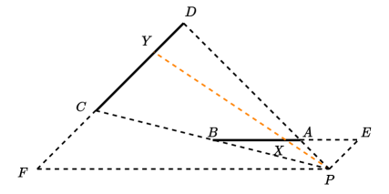
Figure 20: By Lemma 3.10, the value of $|EX||FY|$ is independent of the position of $X$.

As long as $\overleftrightarrow{AB}$ and $\overleftrightarrow{CD}$ are not parallel, Lemma 3.10 will work with any arrangement of the points $A,B,C$ and $D$. Importantly for the $xy\geq 1$ gadget, it is okay if the segments $AB$ and $CD$ intersect. On its own, this lemma could be used to construct a nook which enforces an inversion constraint on two segments which aren’t parallel. Since the input segments to a constraint gadget are parallel, we will need the result of Lemma 3.11 to correct the orientation.

Lemma 3.11.

Suppose line segments $AB$, $CD$, and $EF$ are such that $\overleftrightarrow{AB}$, $\overleftrightarrow{CD}$, and $\overleftrightarrow{EF}$ all intersect at a point $O$, as in Figure 21. Also suppose that the ratios $\frac{|OA|}{|OB|}$ and $\frac{|OC|}{|OD|}$ are the same. Let $P$ be the point where the lines $BE$ and $AF$ intersect, and $Q$ be the point where $DE$ and $CF$ intersect. Draw a line from a point $X$ on $AB$ through $P$, and let $Y$ be the intersection of this line with $EF$. Now draw a line through $Y$ and $Q$. The intersection of this line with $CD$ is $Z$.

Then $\frac{|AX|}{|AB|}=\frac{|CZ|}{|CD|}$.

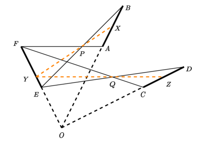
Figure 21: By Lemma 3.11, $\frac{|AX|}{|AB|}=\frac{|CZ|}{|CD|}$.

The proofs of lemmas 3.10 and 3.11 will follow, but first we show how this results give rise to our inversion gadgets. We can now create a nook which enforces an inversion constraint between two parallel segments. Figure 22 shows how to create an $xy\geq 1$ gadget in this way.

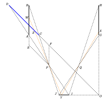
Figure 22: An inversion nook between two parallel segments. The nook attempts to copy between guard segment $GH$ and and the “phantom” segment $CD$, but it ends up hitting segment $AB$ instead. The difference in angle between $CD$ and $AB$ results in inversion.

We choose geometry as in Figure 22 with $|AB|=|GH|$, $\frac{|CD|}{|OD|}=\frac{|GH|}{|OC|}$, $|FD|=4|FC|$, and $|EB|=4|EA|$. By Lemma 3.11 we have $\frac{|GX|}{|GH|}=\frac{|CZ|}{|CD|}$. Since $\frac{|GH|}{|EA|}=\frac{|AB|}{|EA|}=\frac{|CD|}{|FC|}$, we can see that $\frac{|GX|+|EA|}{2|EA|}=\frac{|FZ|}{2|FC|}$, and so by Lemma 3.10 we have that $\frac{|GX|+|EA|}{2|EA|}\cdot\frac{|EZ|}{2|EA|}=\frac{|FZ|}{2|FC|}\cdot\frac{|EZ|}{2|EA|}=1$.

In order to obtain geometry satisfying the required conditions, we choose $CD$ so that it intersects $AB$ a third of the way up with $C$ lying on $\overleftrightarrow{AG}$ and $D$ lying on $\overleftrightarrow{BH}$. From there it is straightforward to complete the geometry.

The $x\left(\frac{5}{2}-y\right)\leq 1$ gadget requires combining these two lemmas in a different way.

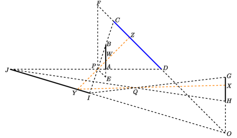
Figure 23: If we reverse the orientation of one segment, we can obtain a constraint like $xy\leq 1$.

Again $|AB|=|GH|$, $|FD|=4|FC|$, and $|EB|=4|EA|$, so $\frac{|GX|+|EA|}{2|EA|}\cdot\frac{EZ}{2|EA|}=1$. The segment $GH$ is now oriented in the reverse direction compared to Figure 22, and the nook is now arranged such that guards see more of the nook segment as $|AZ|$ or $|GX|$ increases. Figure 19 shows the full $x(\frac{5}{2}-y)\leq 1$ gadget.

Constructing an actual instance of this geometry is more difficult than for the $\geq$ inversion gadget. The most direct approaches require solving a quadratic, potentially introducing irrational coordinates. Abrahamsen et al [2] solved a similar issue with their inversion gadgets by carefully choosing coordinates so that the quadratic would have rational solutions. We instead take a geometric approach.

Lemma 3.12.

The geometry in Figure 23 can be chosen so that all vertices have rational coordinates.

Proof.

First, choose the position of the points of points $C$, $D$, $F$, and $P$ such that $|FD|=4|FC|$. Next, choose a point $O$ on $\overleftrightarrow{FD}$ and points $G$ and $H$ so that $\frac{|OH|}{|OG|}=\frac{|OD|}{|OC|}$ and $\overleftrightarrow{GH}$ is parallel to $\overleftrightarrow{FP}$. The points $G$ and $H$ should be chosen to lie below $\overleftrightarrow{PD}$, as in Figure 24.

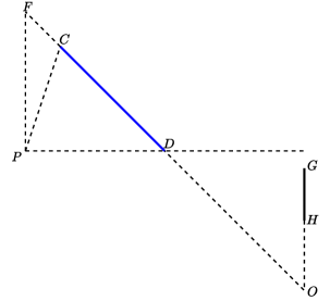
Figure 24:

Next, choose the line segment $AB$ to have length equal to that of $GH$, as in Figure 25.

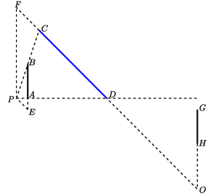
Figure 25:

The remaining points $I$, $J$, and $Q$ can then be placed appropriately. It is straightforward to check that this process doesn’t require introducing irrational coordinates. ∎

The exact geometry used in the final gadget (Figure 19) can be obtained from a setup like Figure 23 by a linear transform.

Proof of Lemma 3.10.

The proof of Lemma 3.10 is a straightforward argument using similar triangles.

The triangles $PEX$ and $PFY$ are similar, so $\frac{|EX|}{|EP|}=\frac{|FP|}{|FY|}$, so $|EX||FY|=|FP||EP|$. In particular, when $X=A$, we have $|EA||FD|=|FP||EP|$, and when $X=B$, we have $|EB||FC|=|FP||EP|$, so $|EA||FD|=|EB||FC|$ and $\frac{|EA|}{|EB|}=\frac{|FC|}{|FD|}$.

Now $|EX||FY|=|FP||EP|=|EA||FD|=|EB||FC|$, so:

$$|EX||FY|=\sqrt{|FP||EP||EB||FC|}=\sqrt{\alpha^{2}\beta^{2}}=\alpha\beta$$

∎

Proof of Lemma 3.11.

Lemma 3.11 could probably be proven using properties of parallelograms, but a linear algebra argument seems more natural.

Place the figure in the vector space $\mathbb{R}^{2}$ with the point $O$ at $(0,0)$. We want to show that there is a linear map which sends points $A,X$ and $B$ to $C,Z$ and $D$ respectively.

The pairs of vectors $\{E,A\}$ and $\{E,C\}$ are each bases for $\mathbb{R}^{2}$. Let $\theta$ be the linear map $\mathbb{R}^{2}\rightarrow\mathbb{R}^{2}$ which takes vector $V$ to $(t,s)$ where $V=tE+sA$, and let $\psi$ be a similar map which writes $V$ as $tE+sC$. Now the linear map $\psi^{-1}\circ\theta$ fixes points on the line containing $E$ and $F$, and sends $A$ to $C$. Since $\frac{|OA|}{|OB|}=\frac{|OC|}{|OD|}$, this map sends $B$ to $D$, and so sends $P$ to $Q$. The point $Y$ is fixed, so the line $\overleftrightarrow{YP}$ is sent to $\overleftrightarrow{YQ}$, meaning that $X$ is sent to $Z$.

So there is a linear map sending points $A,X$ and $B$ to $C,Z$ and $D$ respectively. Since linear maps preserve ratios of distances along a line, we see that:

$$\frac{|AX|}{|AB|}=\frac{|CZ|}{|CD|}$$

∎

Unlike in the parallel copying nooks, the mappings from $AB$ to $EF$ and from $EF$ to $CD$ are in general not linear, only the composition is.

3.8 Addition

The addition constraint is the one constraint that involves more than two variables. A single guard has $2$ coordinates, so a combination of nooks which only interact with $2$ guards each can enforce a constraint which continuously depends on $3$ variables. Figure 26 shows how this is done.

Figure 26: Guards $g_{1}$, $g_{2}$, and $g_{3}$ see parts of the nook segments of nooks $N_{1}$, $N_{2}$, and $N_{3}$ respectively. In order to see the rest of each of these nooks, the guard $g_{4}$ needs to be in the intersection of the shaded triangles (red, green, and purple). This places a constraint on the positions of $g_{1}$, $g_{2}$, and $g_{3}$, since there needs to be at least one point in the intersection of all $3$ regions. The constraint is tight when there is only a single point in this intersection.

The two addition gadgets are shown in Figures 27 and 28. Each has $3$ input segments, and an additional wedge which forms an auxiliary guard region. We don’t need the guard region to control the position of the the auxiliary guard any more precisely than this since the auxiliary guard will have to see parts of all three nook segments.

Figure 27: The $x+y\geq z$ addition gadget. From left to right, the input segments represent the variables $x$, $z$, and $y$.

Figure 28: The $x+y\leq z$ addition gadget. From left to right, the input segments represent variables $z$, $x$, and $y$.

We can use Lemma 3.5 to control the relationship between the positions of the guards on the input segments and their “shadows” on the nook segments, so we just need know how these nooks interact with the auxiliary guard. Lemma 3.13 is used to appropriately determine the geometry of the nooks used.

Lemma 3.13.

Let the line segments $AB$, $CD$, and $EF$ have the same length and lie on the same vertical line, as in Figure 29, and suppose $|CB|=|DE|$. Let points $P$, $Q$, and $R$ lie on a vertical line, with $|QP|=|QR|$. Note that $\overleftrightarrow{AP}$, $\overleftrightarrow{DQ}$, and $\overleftrightarrow{FR}$ intersect in a single point, and the same is true of $\overleftrightarrow{BP}$, $\overleftrightarrow{CQ}$, and $\overleftrightarrow{ER}$.

Choose points $X$ and $Y$ on $AB$ and $EF$ respectively. Now $\overleftrightarrow{XP}$ and $\overleftrightarrow{YQ}$ intersect at a point $I$. Draw a line through points $I$ and $R$. This intersects $CD$ at a point $Z$.

If all is as above, then $\frac{1}{2}\left(|AX|+|EY|\right)=|CZ|$.

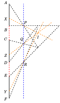
Figure 29: Setup for the addition gadget. By Lemma 3.13, $\frac{1}{2}\left(|AX|+|EY|\right)=|CZ|$.

So if the three nook segments are chosen to have the same length and be equidistant, then we would obtain a constraint like $\frac{1}{2}(x+y)\geq z$. In order to get the constraint $x+y\geq z$, we adjust the middle nook to change the scale and offset of $z$. Figure 30 shows the middle nook from the $x+y\geq z$ gadget. The $x+y\leq z$ gadget is similar.

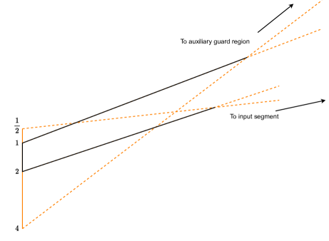
Figure 30: The positions of the auxiliary guard correspond to values of $x+y$ in the range $[1,4]$, while the output segment should correspond to values in the range $[\frac{1}{2},2]$.

The proof of Lemma 3.13 completes the reduction of $\text{ETR-INV}^{rev}$ to the Point-Boundary variant of the art gallery problem, and hence proves Theorem 1.2.

Proof of Lemma 3.13.

We want to transform the geometry from Figure 29 to obtain something like Figure 31.

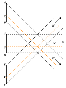
Figure 31: A transformation of the geometry from Figure 29 under which the result of lemma is clear.

This transformation should send straight lines to straight lines and should fix the line containing points $A,B,C,D,E,F,X,Y$ and $Z$. Additionally, the points $P$, $Q$ and $R$ should be sent to infinity, lines through $P$ should be sent to lines with slope $-1$, lines through $Q$ should be sent to lines with slope $0$, and lines through $R$ should be sent to lines with slope $+1$.

If such a transformation exists, then it is clear by elementary linear algebra that $\frac{1}{2}\left(|AX|+|EY|\right)=|CZ|$.

Homographies of $\mathbb{RP}^{2}$ provide a set of transformations which send straight lines to straight lines. A degrees-of-freedom argument is sufficient to show that such a transformation with the required properties exist, but it is not hard to write explicitly. Let $x_{0}$ be the $x$-coordinate of the line containing $A$ and $B$, $x_{1}$ the $x$-coordinate of $P,Q$ and $R$, $y_{0}$ the $y$-coordinate of $Q$, and let $a=|QP|=|QR|$, so $P$ has $y$-coordinate $y_{0}+a$ and $R$ has $y$-coordinate $y_{0}-a$. Then the transformation $(x,y)\rightarrow(x^{\prime},y^{\prime})$ with the desired properties is defined by:

$$\begin{bmatrix}x_{0}+a&0&-(x_{1}+a)x_{0}\\ y_{0}&x_{0}-x_{1}&-y_{0}x_{0}\\ 1&0&-x_{1}\end{bmatrix}\begin{bmatrix}x\\ y\\ 1\end{bmatrix}=\lambda\begin{bmatrix}x^{\prime}\\ y^{\prime}\\ 1\end{bmatrix}$$

Writing the map in this form makes it easy to check what happens to lines through $P$, $Q$, and $R$. In particular, for a $3\times 3$ matrix $A$, if:

$$A\begin{bmatrix}p_{x}\\ p_{y}\\ 1\end{bmatrix}=\begin{bmatrix}a\\ b\\ 0\end{bmatrix}$$

then the map $(x,y)\rightarrow(x^{\prime},y^{\prime})$ given by:

$$\lambda\begin{bmatrix}x^{\prime}\\ y^{\prime}\\ 1\end{bmatrix}=A\begin{bmatrix}x\\ y\\ 1\end{bmatrix}$$

sends lines through $(p_{x},p_{y})$ to lines parallel to $\begin{bmatrix}a\\ b\end{bmatrix}$.

∎

Abrahamsen et al [2] use an instance of the same type of geometry for their addition gadget. The verification of their gadget given in that paper could be generalized to give a different proof of Lemma 3.13.

4 Conclusions

While the complexity of Boundary-Boundary variant of the art-gallery problem is still unresolved, our result shows that the X-Y and Y-X variants of the art gallery problem are equivalent under polynomial time reductions when $X,Y\in\{\text{Vertex},\text{Point},\text{Boundary}\}$ (Corollary 1.3). Visibility is reflexive, so this result seems unsurprising. Perhaps it could be proven more directly.

It is interesting to note that our construction, while intended for the Point-Boundary variant of the art gallery problem, is also sufficient to show the $\exists\mathbb{R}$-hardness of the standard Point-Point variant. Indeed, all the guarding configurations considered are also guarding configurations in the Point-Point variant. This is similar to the construction from [2], which simultaneously showed the $\exists\mathbb{R}$-hardness of the Point-Point and Boundary-Point variants. It doesn’t seem to be possible to adapt either construction to the Boundary-Boundary variant.

In our construction, each nook enforces a constraint between only two guards. While it is possible to put multiple guard regions in the critical region of one nook, the types of constraints created seem to be unable to depend continuously on more than $2$ of the guards at a time. Addition constraints are only possible because the guards themselves have two coordinates, so a single nook can in principle enforce a constraint on as many as $4$ variables. In the Boundary-Point variant, guards have only one coordinate, but have to cover the entire $2$-dimensional interior of the art gallery, so constraints that continuously depend on the positions of more than $2$ guards can be created. In the Boundary-Boundary variant, neither of these ideas work, so it seems unlikely that a problem like ETR-INV could be reduced to it in this way. It is very possible that the Boundary-Boundary variant is only NP.

5 Acknowledgements

I am grateful to Eric Stade, Elisabeth Stade, Jamie Tucker-Foltz, Tillman Miltzow and Mikkel Abrahamsen for feedback on drafts of this paper.

References

- [1] Mikkel Abrahamsen, Anna Adamaszek, and Tillmann Miltzow. Irrational guards are sometimes needed. 01 2017.
- [2] Mikkel Abrahamsen, Anna Adamaszek, and Tillmann Miltzow. The art gallery problem is -complete. In Proceedings of the 50th Annual ACM SIGACT Symposium on Theory of Computing, STOC 2018, Los Angeles, CA, USA, June 25-29, 2018, pages 65–73, 2018.
- [3] Mikkel Abrahamsen, Tillmann Miltzow, and Nadja Seiferth. Framework for er-completeness of two-dimensional packing problems. pages 1014–1021, 11 2020.
- [4] Akanksha Agrawal, Kristine V. K. Knudsen, Daniel Lokshtanov, Saket Saurabh, and Meirav Zehavi. The Parameterized Complexity of Guarding Almost Convex Polygons. In Sergio Cabello and Danny Z. Chen, editors, 36th International Symposium on Computational Geometry (SoCG 2020), volume 164 of Leibniz International Proceedings in Informatics (LIPIcs), pages 3:1–3:16, Dagstuhl, Germany, 2020. Schloss Dagstuhl–Leibniz-Zentrum für Informatik.
- [5] Daniel Bertschinger, Nicolas El Maalouly, Tillmann Miltzow, Patrick Schnider, and Simon Weber. Topological art in simple galleries. In Symposium on Simplicity in Algorithms (SOSA), pages 87–116. Society for Industrial and Applied Mathematics, jan 2022.
- [6] Édouard Bonnet and Tillmann Miltzow. An approximation algorithm for the art gallery problem. In SoCG, 2017.
- [7] John Canny. Some algebraic and geometric computations in pspace. In Proceedings of the Twentieth Annual ACM Symposium on Theory of Computing, STOC ’88, page 460–467, New York, NY, USA, 1988. Association for Computing Machinery.
- [8] Aldo Laurentini. Guarding the walls of an art gallery. The Visual Computer, 15:265–278, 10 1999.
- [9] D. T. Lee and Arthur K. Lin. Computational complexity of art gallery problems. IEEE Transactions on Information Theory, 32(2):276–282, 1986.
- [10] Tillmann Miltzow and Reinier F. Schmiermann. On classifying continuous constraint satisfaction problems. In 2021 IEEE 62nd Annual Symposium on Foundations of Computer Science (FOCS), pages 781–791, 2022.
- [11] Nikolai E Mnëv. The universality theorems on the classification problem of configuration varieties and convex polytopes varieties. In Topology and geometry—Rohlin seminar, pages 527–543. Springer, 1988.
- [12] Joseph O’Rourke. Art gallery theorems and algorithms, volume 57. Oxford New York, NY, USA, 1987.
- [13] Marcus Schaefer and Daniel Stefankovic. Fixed points, nash equilibria, and the existential theory of the reals. Theory of Computing Systems, 60:172–193, 2017.
- [14] Marcus Schaefer and Daniel Stefankovic. Beyond the existential theory of the reals, 2022.
- [15] Peter W. Shor. Stretchability of pseudolines is np-hard. In Applied Geometry And Discrete Mathematics, 1990.
- [16] Jack Stade and Jamie Tucker-Foltz. Topological universality of the art gallery problem, 2022.