Simple Alternating Minimization Provably Solves Complete Dictionary Learning

Abstract

This paper focuses on complete dictionary learning problem, where the goal is to reparametrize a set of given signals as linear combinations of atoms from a learned dictionary. There are two main challenges faced by theoretical and practical studies of dictionary learning: the lack of theoretical guarantees for practically-used heuristic algorithms, and their poor scalability when dealing with huge-scale datasets. Towards addressing these issues, we show that when the dictionary to be learned is orthogonal, that an alternating minimization method directly applied to the nonconvex and discrete formulation of the problem exactly recovers the ground truth. For the huge-scale, potentially on-line setting, we propose a minibatch version of our algorithm, which can provably learn a complete dictionary from a huge-scale dataset with minimal sample complexity, linear sparsity level, and linear convergence rate, thereby negating the need for any convex relaxation for the problem. Our numerical experiments showcase the superiority of our method compared with the existing techniques when applied to tasks on real data.

1 Introduction

We consider the following optimization problem:

$$\min_{\bm{X},\bm{D}}\|\bm{Y}-\bm{D}\bm{X}\|_{F}^{2}+\zeta\|\bm{X}\|_{0},$$ (DL)

where $\bm{Y}\in\mathbb{R}^{n\times p}$ commonly denotes a data matrix whose columns are observed signals. Given $\bm{Y}$, our goal is to find a dictionary $\bm{D}\in\mathbb{R}^{n\times k}$ and the corresponding code $\bm{X}\in\mathbb{R}^{k\times p}$ such that: (1) each signal in $\bm{Y}$ is approximately represented as a linear combination of columns (also called atoms) of $\bm{D}$; and (2) such representation uses as few atoms as possible. In other words, we require columns of $\bm{X}$ to be sparse, which means a large portion of entries in $\bm{X}$ should be zero. Here, the pseudo-norm $\|\cdot\|_{0}$ counts the number of non-zero entries in $\bm{X}$ and is being used as a regularizer to promote sparsity.

Problem DL is widely known as the dictionary learning problem. The optimal dictionary $\bm{D}^{*}$ computed from DL gives an optimally-sparse representation of the data (Donoho and Elad, (2003)), and its columns have a natural interpretation as a set of feature vectors that “best explain the data.” As such, Problem DL arises ubiquitously across numerous application domains, ranging from clustering and classification (Ramirez et al., (2010); Tošić and Frossard, (2011)), to image, audio, and video processing (Mairal et al., (2007); Liu et al., (2018); Grosse et al., (2012)), to facial recognition (Xu et al., (2017)), to medical imaging (Zhao et al., (2021)), and to many others.

Perhaps the most widely-used heuristic for solving DL is based on alternating minimization: to solve for the sparse code by fixing the dictionary, and then use the resulting code to update the dictionary. Examples of this method are the Method of Optimal Direction (MOD, Engan et al., (1999)) and KSVD (Aharon et al., (2006)). However, despite their simplicity, the methods based on alternating minimization are faced with two major challenges:

Lack of theoretical guarantees:

Due to the nonconvexity of DL stemming from the nonlinear term $\bm{D}\bm{X}$ and discrete regularizer $\|\bm{X}\|_{0}$, methods like MOD and KSVD are poorly understood on the theoretical side. As a result, their recovered solution may be arbitrarily far from the sparsest representation of the signal, which is a serious concern in applications where efficient and provable sparse representation of the data is crucial.

Limited scalability and incompatibility with on-line learning:

Existing methods become intractable for modern “big data” applications, such as high-resolution image processing (Ayas and Ekinci, (2020)) and video processing (Haq et al., (2020)), whose datasets are huge-scale and often dynamically generated, and for which processing must be performed essentially in real-time. Consider the task of image processing as an example. In order to learn a dictionary from more than 10000 images, the existing state-of-the-art (namely, the KSVD method) has to first reduce the sample size to a few hundreds through down-sampling and then divide the images into block patches of $8\times 8$ pixels (Aharon et al., (2006)). Moreover, when newly-generated data arrive, there is no mechanism within the algorithm that allows for the dictionary to be incrementally improved, other than to run the algorithm from scratch again. As a result, the lack of scalability of the algorithm severely undermines the quality of dictionary and may lead to serious ramifications in applications like medical imaging.

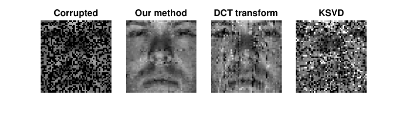
Figure 1: A comparison of image denosing using our proposed method (Algorithm 3), KSVD and DCT. We choose a random image and artificially corrupt 50% of the pixels. Reconstruction is done via orthogonal matching pursuit, using the learned dictionaries. Here we use 35 atoms, which corresponds to a sparsity level of 35%. The corrupted original image is plotted in the left hand side, and the three reconstructed images are shown on the right. We see the our method achieves a much better denoising result than both KSVD and DCT.

1.1 Our Contribution

In this work, we assume the data matrix $\bm{Y}$ is generated as $\bm{Y}=\bm{D}^{*}\bm{X}^{*}$ where $\bm{D}^{*}\in\mathbb{R}^{n\times n}$ is a square dictionary whose columns are the true atoms and $\bm{X}^{*}$ is a sparse code matrix. We consider scenarios where the true dictionary $\bm{D}^{*}$ is assumed to be orthogonal or a general non-singular matrix. The former is commonly referred to as orthonormal dictionary learning (ODL), while the later is known as complete dictionary learning (CDL) in the literature (Sun et al.,, 2015; Zhai et al.,, 2020). Specifically, towards solving DL in such settings, we make the following contributions:

1. Provable convergence: We first consider the simplest and most intuitive alternating minimization scheme on DL, where we alternatingly fix one variable and optimize DL with respect to the other. We prove that for ODL, this simple algorithm provably recovers both $\bm{X}^{*}$ and $\bm{D}^{*}$. Then, we propose an extension to CDL through a carefully designed preconditioner based on Cholesky factorization. We show the provable scalability of our method in both huge-scale and online settings.

2. Statistical guarantee: Our methods enjoy promising statistical guarantees compared to the existing work. In particular, our algorithm converges to the ground truth under the assumption that a constant fraction of the entries in the sparse code matrix is non-zero, a sparsity level which is not reached by previous alternating minimization methods to the best of our knowledge.

3. Practical performance: We showcase the effectiveness and scalability of our algorithms through practical tasks of image denoising and image reconstruction on large dataset. We show that our method beats the state-of-the-art methods in both performance and efficiency, as illustrated in Figure 1 and Section 4.

1.2 Notation

In this paper, we use $a$ or $\alpha$ to denote scalars, $\bm{a}$ to denote vectors and $\bm{A}$ do denote matrices. We use $\bm{A}_{(i,\cdot)}$ to denote the $i$th row of $\bm{A}$ and $\bm{A}_{(\cdot,j)}$ to denote the $j$th column of $\bm{A}$. We use $\|\bm{A}\|_{2}$ to denote the spectral norm of $\bm{A}$, $\|\bm{A}\|_{F}$ to denote Frobenius norm of $\bm{A}$, $\|\bm{A}\|_{2,\infty}$ to denote the maximum column norm of $\bm{A}$, $\|\bm{A}\|_{0}$ to denote the total number of non-zero entries in $\bm{A}$, and $\|\bm{A}\|_{1}$ to denote the entry-wise $\ell_{1}$ norm of $\bm{A}$. We use $\bm{I}_{d}$ to denote the $d\times d$ identity matrix, and $\mathbb{O}(n)$ to denote the orthogonal group in dimension $n$. We use $\mathrm{supp}(\bm{A})$ to denote the set of indices of non-zero entries of $\bm{A}$. We define the hard-thresholding operator $\mathrm{HT}_{\zeta}(\cdot)$ at level $\zeta$ as:

$$\left(\mathrm{HT}_{\zeta}(\bm{A})\right)_{(i,j)}=\begin{cases}\bm{A}_{(i,j)}&\text{if}\quad|\bm{A}_{(i,j)}|\geq\zeta\\ 0&\text{if}\quad|\bm{A}_{(i,j)}|<\zeta\\ \end{cases}.$$ (1)

We use $\sigma_{i}(\bm{A})$ to denote the $i$th largest singular value of $\bm{A}$ and $\kappa(\bm{A})$ to denote the condition number of $\bm{A}$. We define the operator $\mathrm{Polar}(\bm{A})=\bm{U}_{\bm{A}}\bm{V}_{\bm{A}}^{\top}$, where $\bm{U}_{\bm{A}}\bm{\Sigma}_{\bm{A}}\bm{V}_{\bm{A}}^{\top}$ is the Singular Value Decomposition (SVD) of $\bm{A}$. We also define the operator $\mathcal{L}(\bm{A})=\bm{L}_{\bm{A}}$, where $\bm{L}_{\bm{A}}\bm{L}_{\bm{A}}^{\top}$ is the Cholesky factorization of a positive semidefinite matrix $\bm{A}$. We use $f(x)=O(g(x))$ when $f(x)\leq Cg(x)$ for all large enough $x$ and some universal constant $C$. We use $f(x)=\Omega(g(x))$ if $g(x)=O(f(x))$. To streamline the presentation, we say an event happens with high probability if it occurs with probability of at least $1-n^{\Omega(1)}$ with respect to all the randomness in the problem, provided that both the sample size and the number of iterations of the algorithm are upper bounded by some polynomial function of $n$.

1.3 Organization

The paper is organized as follows. In Section 2, we provide a survey of related research work on sparse dictionary learning problem. Then, we introduce our main results in Section 3. We conclude our paper with numerical experiments in Section 4. All the detailed proofs are deferred to the appendix.

2 Related Work

Since the seminal work of Olshausen and Field, (1996), there have been many exciting and inspirational research outcomes in the study of dictionary learning. Here, we provide a brief review on results that are most related to this paper.

The ground truth as the globally-optimal solution:

As the first question, we must first verify whether the ground truth $(\bm{D}^{*},\bm{X}^{*})$ is indeed the global minimizer of DL for the generative model $\bm{Y}=\bm{D}^{*}\bm{X}^{*}$. Of course, if this were not the case, then solving DL—even to global optimality—may not be enough to actually recover the ground truth $(\bm{D}^{*},\bm{X}^{*})$. A series of work by Gribonval and Schnass, (2010); Geng and Wright, (2014); Jenatton et al., (2012); Schnass, (2015) studied the local optimality of the ground truth for DL by replacing $\ell_{0}$ norm with $\ell_{1}$ norm. Spielman et al., (2012) elegantly showed that the ground truth is the unique global minimizer to DL when $\zeta\rightarrow 0$. Specifically, when $p=\Omega(n\log n)$, they showed that $(\bm{X}^{*},\bm{D}^{*})$ is the global minimizer to $\min_{\bm{X},\bm{D}}\|\bm{X}\|_{0}$ subject to the constraint $\bm{Y}=\bm{D}\bm{X}$. The question remains to be answered is how to find a provable algorithm to recover $\bm{X}^{*}$ and $\bm{D}^{*}$.

Provable guarantee for alternating minimization:

The empirical success achieved by methods like MOD and KSVD has encouraged the emergence of many alternating minimization algorithms (Lee et al., (2006); Mairal et al., (2009); Bao et al., (2013, 2014)). However, theoretical gaps remain in our understanding of why such algorithms can work so well. Currently, the best guarantees that have been obtained for the aforementioned algorithms are limited to the convergence to a critical point. Towards providing a provable guarantee for alternating minimization, Agarwal et al., (2016) give a theoretical analysis for a specific type of alternating minimization method by replacing the $\ell_{0}$ pseudo-norm with its convex surrogate $\ell_{1}$ norm. Their proposed algorithm solves a LASSO problem in each iteration and relies on a restricted isometry property (RIP) assumption. Arora et al., (2015) considers a general framework where sparse coding can be solved by hard thresholding with a predetermined threshold and dictionary is updated by a gradient descent step with the sparse code fixed. However, their proof breaks down when the sparsity level exceeds $O(\sqrt{n})$. Ravishankar et al., (2020) propose an alternating scheme based on the assumption that each sparse code has equal non-zero entries. Despite their strong provable guarantees, none of these papers provide any experiment on real dataset.

Other method with provable guarantee:

Barak et al., (2015) adopt and analyze the Sum of Squares semidefinite programming hierarchy to solve DL. Recent years have also witnessed the trend of analyzing the dictionary learning problem via the Riemann manifold perspective (Sun et al., (2015); Qu et al., (2014); Zhai et al., (2020)). However, the applicability of such methods to real data has remained elusive since little empirical evidence is provided in their work. Inspired by recent results on the benign landscape of matrix factorization problems (Ge et al.,, 2016, 2017; Fattahi and Sojoudi,, 2020), Sun et al., (2016) have shown that a smoothed variant of DL is devoid of spurious local solutions.

3 Our Method

As fundamental as DL is to data analysis and signal processing, it is dauntingly non-convex. There are two sources of non-convexity in the formulation of DL and they are dealt with in different ways on the algorithmic side: the first difficulty is the bi-linearity induced by the term $\bm{D}\bm{X}$, which inspires the strategy of alternating minimization. The second difficulty originates from the pseudo-norm $\|\cdot\|_{0}$, which is non-convex and discrete. To circumvent this issue, the common approach is to replace $\|\cdot\|_{0}$ with its convex surrogate $\|\cdot\|_{1}$ (Mairal et al., (2009)Agarwal et al., (2016)), which in turn leads to inferior statistical guarantees (Fan and Li, (2001)Zhang, (2010)). Our main result is to show that such relaxation is not needed, since a tailored alternating minimization can provably recover the true solution of DL at scales that were not possible before. We first introduce a simple algorithm for the orthogonal dictionary learning. Then, we extend our algorithm to the more general case of complete dictionary learning and its online variant, where the data is processed dynamically over time.

3.1 Full-batch Orthogonal Dictionary Learning

We first assume the dictionary to be an orthogonal matrix $\bm{D}^{*}\in\mathbb{O}(n)$, in which case the problem is termed as Orthogonal Dictionary Learning (ODL):

$$\min_{\bm{D}\in\mathbb{O}(n),\bm{X}}\|\bm{Y}-\bm{D}\bm{X}\|_{F}^{2}+\zeta\|\bm{X}\|_{0}.$$ (ODL)

Towards solving ODL, we consider the following alternating minimization scheme:

• Step 1: Fix $\bm{D}^{(t)}$, update $\bm{X}^{(t)}=\arg\min_{\bm{X}\in\mathbb{R}^{n\times p}}\|\bm{Y}-\bm{D}^{(t)}\bm{X}\|_{F}^{2}+\zeta\|\bm{X}\|_{0}$.

• Step 2: Fix $\bm{X}^{(t)}$, update $\bm{D}^{(t+1)}=\arg\min_{\bm{D}\in\mathbb{O}(n)}\|\bm{Y}-\bm{D}\bm{X}^{(t)}\|_{F}^{2}+\zeta\|\bm{X}^{(t)}\|_{0}$.

It is easy to see that both steps of the algorithm have closed-form solutions that can be efficiently calculated. In particular, Step 1 is equivalent to finding the proximal operator of $\ell_{0}$ norm at the reference point $\bm{D}^{(t)\top}\bm{Y}$, which can be obtained by hard-thresholding the entries of $\bm{D}^{(t)\top}\bm{Y}$ at level $\zeta$. Step 2 reduces to the famous Procrustes problem, for which the optimal solution is obtained via the polar decomposition $\bm{D}^{(t+1)}=\mathrm{Polar}\left(\bm{Y}\bm{X}^{(t)\top}\right)$. This leads to the following alternating minimization algorithm:

Algorithm 1 Alternating minimization for ODL

1:  Input: $\bm{Y}$, $\bm{D}^{(0)}$, $\zeta$

2:  for $t=0,1,\dots,T$ do

3:     Set $\bm{X}^{(t)}=\mathrm{HT}_{\zeta}\left(\bm{D}^{(t)\top}\bm{Y}\right)$

4:     Set $\bm{D}^{(t+1)}=\mathrm{Polar}\left(\bm{Y}\bm{X}^{(t)\top}\right)$

5:  end for

6:  return  $\bm{D}^{(T)}$,$\bm{X}^{(T)}$

We note that Algorithm 1 has been studied before. Bao et al., (2013) report their empirical observation that Algorithm 1 achieves considerable efficiency in image restoration. In Ravishankar et al., (2020), authors provide a theoretical analysis for a variant of Algorithm 1 based on sorted thresholding. One may even argue that Algorithm 1 is similar to the Method of Optimal Directions (MOD). However, the existing theoretical guarantees for Algorithm 1 are very restrictive.

To bridge this knowledge gap, we first introduce our assumption on the sparse matrix $\bm{X}$.

Assumption 1 (Model for Sparse Code Matrix).

The sparsity pattern of ground truth $\bm{X}^{*}$ is drawn from an independent Bernoulli distribution with parameter $\theta=(0,1]$. In particular, for each entry $1\leq i\leq n$, $1\leq j\leq p$,

$$\mathbbm{1}_{\bm{X}^{*}_{ij}\neq 0}=B_{ij}\quad\text{where}\quad B_{ij}\overset{i.i.d.}{\sim}\mathcal{B}(\theta).$$ (2)

Moreover, the non-zero values of $\bm{X}^{*}$ are drawn from an i.i.d zero-mean and finite-variance sub-Gaussian random variables. We also assume the magnitudes of non-zero entries of $\bm{X}^{*}$ are lower bounded by some constant $\Gamma$. More specifically, for every $(i,j)\in\mathrm{supp}(\bm{X}^{*})$, we have

$$|\bm{X}^{*}_{ij}|\geq\Gamma,\quad\mathbb{E}(\bm{X}^{*}_{ij})=0,\quad\text{and}\quad\mathbb{E}(\bm{X}^{*2}_{ij})=\sigma^{2}.$$ (3)

Now, we are ready to show the convergence of Algorithm 1:

Theorem 1.

Suppose that Assumption 1 holds with sparsity level $\theta\leq\frac{1}{144}$, and the initial dictionary $\bm{D}^{(0)}$ satisfies $\|\bm{D}^{(0)}-\bm{D}^{*}\|_{F}\leq O(1/\log n)$. Moreover, suppose that the sample size satisfies $p\geq\Omega\left(n/\theta^{2}\right)$. Then, with high probability, the iterations of Algorithm 1 with $\zeta=\Gamma/2$ satisfy:

$$\|\bm{D}^{(t)}-\bm{D}^{*}\|_{F} \leq(1/2)^{t}\|\bm{D}^{(0)}-\bm{D}^{*}\|_{F}$$ (4)

$$\|\bm{X}^{(t)}-\bm{X}^{*}\|_{F} \leq(1/2)^{t}\|\bm{X}^{(0)}-\bm{X}^{*}\|_{F}$$ (5)

Theorem 1 improves upon the existing results on two fronts:

Linear sparsity level:

We allow a constant fraction of entries in $\bm{X}^{*}$ to be non-zero, thereby improving upon the best known sparsity level of $O(\sqrt{n}/\log n)$ for alternating minimization (Arora et al.,, 2015).

Linear sample complexity:

In order to recover $\bm{D}^{*}$ exactly, we only need to observe $O(n)$ many samples, which is even one $\log(n)$ factor smaller than the sample complexity required for the uniqueness of the solution when $\xi\rightarrow 0$ (Spielman et al., (2012)). Note that this sample complexity is optimal (modulo constant factors), since it is impossible to recover the true dictionary with sublinear number of samples even if $X^{*}$ is known.

Even though our result is built on a quite generous initialization requirement $\|\bm{D}^{(0)}-\bm{D}^{*}\|_{F}\leq O(1/\log n)$, we suspect that it can be potentially improved to $\|\bm{D}^{(0)}-\bm{D}^{*}\|_{2,\infty}\leq O(1/\log n)$, which is the best known convergence radius for alternating minimization (Arora et al.,, 2015).

Despite its desirable sample complexity and convergence rate, Algorithm 1 suffers from two fundamental limitations. First, its convergence is contingent upon the orthogonality of the true dictionary, which is not satisfied in a lot of applications. Second, it does not readily extend to huge-scale or online settings, where it is prohibitive or impossible to process all samples at once. To address these challenges, we extend our algorithm to complete (non-orthogonal) dictionary learning with mini-batch and online data in the next two subsections.

3.2 Mini-batch Complete Dictionary Learning

We move on to generalize Algorithm 1 to CDL with huge sample size. To distinguish from ODL, we denote the ground truth dictionary as $\bm{A}^{*}$ (i.e., $\bm{Y}=\bm{A}^{*}\bm{X}^{*}$). Towards dealing with large $p$, the strategy adopted here is to sub-sample from the columns of $\bm{Y}$. To address the non-orthogonality of the dictionary, we consider a preconditioner based on Cholesky factorization. In particular, we define a preconditioner $\bm{P}$ as

$$\bm{P}=\mathcal{L}\left(\left(\frac{1}{p\theta\sigma^{2}}\bm{Y}\bm{Y}^{\top}\right)^{-1}\right)^{\top},$$ (6)

and obtain a new (preconditioned) data matrix $\tilde{\bm{Y}}=\bm{P}\bm{Y}$. To explain the intuition behind this choice of preconditioner, note that $\frac{1}{p\theta\sigma^{2}}\bm{Y}\bm{Y}^{\top}\approx\bm{A}^{*}\bm{A}^{*\top}$ for large enough $p$, which allows us to write $\tilde{\bm{Y}}\approx\mathcal{L}\left(\left(\bm{A}^{*}\bm{A}^{*\top}\right)^{-1}\right)^{\top}\bm{A}^{*}\bm{X}^{*}$. Upon defining $\bm{D}^{*}=\mathcal{L}\left(\left(\bm{A}^{*}\bm{A}^{*\top}\right)^{-1}\right)^{\top}\bm{A}^{*}$, one can check that $\bm{D}^{*}\in\mathbb{O}(n)$ and $\tilde{\bm{Y}}=\bm{D}^{*}\bm{X}^{*}$. Indeed, this is an instance of ODL and can be solved using Algorithm 1. Therefore, we propose the following algorithm for solving CDL:

Algorithm 2 Alternating minimization for mini-batch CDL

1:  Input: $\bm{Y}$, $\bm{A}^{(0)}$, $\zeta$

2:  Set $\bm{P}=\mathcal{L}\left(\left(\frac{1}{p\theta\sigma^{2}}\bm{Y}\bm{Y}^{\top}\right)^{-1}\right)^{\top}$.

3:  Set $\tilde{\bm{Y}}=\bm{P}\bm{Y}$.

4:  Set $\bm{D}^{(0)}=\mathcal{L}\left(\left(\bm{A}^{(0)}\bm{A}^{{0}\top}\right)^{-1}\right)^{\top}\bm{A}^{(0)}$.

5:  for $t=0,1,\dots,T-1$ do

6:     Sample $\tilde{p}$ many columns from $\tilde{\bm{Y}}$ to be $\tilde{\bm{Y}}^{(t)}$.

7:     Set $\tilde{\bm{X}}^{(t)}=\mathrm{HT}_{\zeta}\left(\bm{D}^{(t)\top}\tilde{\bm{Y}}^{(t)}\right)$.

8:     Set $\bm{D}^{(t+1)}=\mathrm{Polar}\left(\tilde{\bm{Y}}^{(t)}\tilde{\bm{X}}^{(t)\top}\right)$.

9:  end for

10:  return  $\bm{P}^{-1}\bm{D}^{(T)}$ as an approximation to $\bm{A}^{*}$

Our next theorem characterizes the performance of Algorithm 2. To better present our result, we consider $\bm{A}^{(t)}$ to be the output of the algorithm if it stops at $t$th iteration. Without loss of generality, we assume that $\|\bm{A}^{*}\|_{2}=1$ and set $\hat{\kappa}$ to be the condition number of $\bm{A}^{*}$.

Theorem 2.

Suppose Assumption 1 holds with sparsity level $\theta\leq\frac{1}{5600}$, and the initial dictionary $\bm{A}^{(0)}$ satisfies $\|\bm{A}^{(0)}-\bm{A}^{*}\|_{F}\leq O(1/(\hat{\kappa}^{6}\log n))$. Moreover, suppose that the sample size and batch size satisfy $p\geq\Omega(n^{2}\log n\sigma^{2}\hat{\kappa}^{12}/(\theta^{2}\Gamma))$ and $\tilde{p}\geq\Omega\left(n/\theta^{2}\right)$. Then, with high probability and for some $0<\rho<1$, the iterations of Algorithm 2 with $\zeta=\Gamma/2$ satisfy:

$$\left\|\bm{A}^{(t)}-\bm{A}^{*}\right\|_{F}\leq \ \rho^{t}\|\bm{A}^{(0)}-\bm{A}^{*}\|_{F}+O\left(\frac{n\hat{\kappa}^{6}}{\theta\sqrt{p}}\right).$$ (7)

Theorem 2 states that Algorithm 2 converges linearly to the true dictionary up to a statistical error of $O\left(\frac{n\hat{\kappa}^{6}}{\theta\sqrt{p}}\right)$. This statistical error is due to the deviation of the preconditioner from its expectation, which diminishes with $p$. A noticeable difference between our result and other results is that we do not impose any incoherency requirement or restricted isometry property on $\bm{A}^{*}$, which are prevalent in existing results, especially for algorithms that use $\ell_{1}$ relaxation.

Finally, note that Algorithm 2 does not return the code matrix $\bm{X}^{*}$. This is due to the fact that our proposed algorithm may not see all the samples. More precisely, it will see $\tilde{p}T$ samples by iteration $T$, which can be significantly smaller than the full sample size $p$. Therefore, Algorithm 2 cannot recover the full code matrix. However, given an approximation $\bm{A}^{(t)}$ of $\bm{A}^{*}$, the sparse code corresponding to any sample $\bm{Y}^{(s)}$ can be readily recovered by computing $\bm{X}^{(s)}=\mathrm{HT}_{\zeta}\left(\left(\bm{P}\bm{A}^{(t)}\right)^{\top}\bm{P}\bm{Y}^{(s)}\right)$.

3.3 Online Dictionary Learning

Even though the computational efficiency of Algorithm 2 is largely improved compared to its full-batch counterpart, we still may face the following challenges in reality. First, the sample size $p$ is so large that even a one-time calculation of the preconditioner $\bm{P}$ is unrealistic. Second, samples (columns of $\bm{Y}$) may arrive dynamically over time. Both situations call for an efficient method to update the preconditioner more efficiently in an online setting.

To update $\bm{P}$ with a new sample $\bm{y}$, a naive approach would be to re-compute it from scratch which would cost $O(n^{3})$ operations. However, we show that $\bm{P}$ can be updated more efficiently in $O(n^{2})$ operations by taking advantage of the more efficient rank-one updates on matrix inversion and Cholesky factorization. To this goal, we first use the Sherman-Morrison formula to update $\left(\bm{Y}\bm{Y}^{\top}\right)^{-1}$ as

$$\left(\bm{Y}\bm{Y}^{\top}+\bm{y}\bm{y}^{\top}\right)^{-1}=\left(\bm{Y}\bm{Y}^{\top}\right)^{-1}-\bm{v}\bm{v}^{\top},\quad\text{where}\quad\bm{v}=\left(1+\bm{y}^{\top}\left(\bm{Y}\bm{Y}^{\top}\right)^{-1}\bm{y}\right)^{-1/2}\left(\bm{Y}\bm{Y}^{\top}\right)^{-1}\bm{y},$$

which, given $\left(\bm{Y}\bm{Y}^{\top}\right)^{-1}$, can be obtained in $O(n^{2})$ operations. Given the above rank-one update for the inverse, the Cholesky factor $\mathcal{L}\left(\left(\bm{Y}\bm{Y}^{\top}+\bm{y}\bm{y}^{\top}\right)^{-1}\right)$ can be obtained within $O(n^{2})$ operations by performing triangular rank-one updates on $\mathcal{L}\left(\left(\bm{Y}\bm{Y}^{\top}\right)^{-1}\right)$ (Krause and Igel,, 2015). We explain the precise implementation of these updates in Appendix D.

Inspired by the above update, we propose Algorithm 3 for solving online dictionary learning. We start the algorithm by initializing the inverse of the data matrix (denoted as $\bm{Z}^{(t)}_{\text{inv}}$) and the preconditioner using $p_{1}$ samples. Moreover, we use $p_{2}$ samples for our initial data set. When a new sample arrives, we update the preconditioner $\bm{P}^{(t)}$ and $\bm{Z}^{(t)}_{\text{inv}}$ via the triangular rank-one update explained in Appendix D, and update the data set accordingly. Then, we perform the alternating minimization as presented before using the new data set and the new preconditioner.

Algorithm 3 Alternating minimization for online dictionary learning

1:  Input: $\bm{A}^{(0)}_{0}$, $\zeta$, $p_{1}$,$p_{2}$

2:  Construct the data matrix $\bm{Y}$ with $p_{1}$ samples and set $\bm{Z}^{(0)}_{\text{inv}}=\left(\bm{Y}\bm{Y}^{\top}\right)^{-1}$ and $\bm{P}^{(0)}=\mathcal{L}\left({p_{1}\theta\sigma^{2}}\bm{Z}^{(0)}_{\text{inv}}\right)^{\top}$.

3:  Initialize $\bm{Y}^{(0)}$ with $p_{2}$ samples.

4:  for $t=0,1,\dots,T-1$ do

5:     Get new vector $\bm{y}$.

6:     Set $\bm{Y}^{(t)}=[\bm{Y}^{(t-1)}\quad\bm{y}]$.

7:     Remove first column of $\bm{Y}^{(t)}$.

8:     Update $\bm{P}^{(t)}$ and $\bm{Z}^{(t)}_{\text{inv}}$ with $\bm{P}^{(t-1)}$, $\bm{Z}^{(t-1)}_{\text{inv}}$, and new $\bm{y}$ using Algorithm 5 in Appendix D.

9:     Set $\tilde{\bm{Y}}^{(t)}=\bm{P}^{(t)}\bm{Y}^{(t)}$

10:     Set $\tilde{\bm{X}}^{(t)}=\mathrm{HT}_{\zeta}\left(\bm{D}^{(t)\top}\tilde{\bm{Y}}^{(t)}\right)$.

11:     Set $\bm{D}^{(t+1)}=\mathrm{Polar}\left(\tilde{\bm{Y}}^{(t)}\tilde{\bm{X}}^{(t)\top}\right)$.

12:  end for

13:  return  $\left(\bm{P}^{(T-1)}\right)^{-1}\bm{D}^{(T)}$ as an approximation to $\bm{A}^{*}$

Our next theorem establishes the convergence of Algorithm 3 for the online dictionary learning.

Theorem 3.

Suppose that Assumption 1 holds with the sparsity level $\theta\leq\frac{1}{5600}$, and the initial dictionary $\bm{A}^{(0)}$ satisfies $\|\bm{A}^{(0)}-\bm{A}^{*}\|_{F}\leq O(1/(\hat{\kappa}^{6}\log n))$. Moreover, suppose that we have $p_{1}\geq\Omega(n^{2}\log n\sigma^{2}\hat{\kappa}^{12}/(\theta^{2}\Gamma))$ and $p_{2}\geq\Omega\left(n/\theta^{2}\right)$. Then, with high probability and for some $0<\rho<1$, the iterations of Algorithm 3 with $\zeta=\Gamma/2$ satisfy:

$$\left\|\bm{A}^{(t)}-\bm{A}^{*}\right\|_{F}\leq \ \rho^{t}\|\bm{A}^{(0)}-\bm{A}^{*}\|_{F}+O\left(\frac{n\hat{\kappa}^{6}}{\theta\sqrt{p_{1}+t}}\right).$$ (8)

The convergence result of Algorithm 3 is similar to that of Algorithm 2, with a key difference that the statistical error term $O\left(\frac{n\hat{\kappa}^{6}}{\theta\sqrt{p_{1}+t}}\right)$ now decreases with $t$, which is due to the fact that the preconditioner is updated with a new sample at every iteration.

3.4 Discussion

3.4.1 Initialization

The theoretical success of Algorithms 1-3 requires, at least in theory, a good initialization with $O(1/\log n)$ distance to the ground truth. Such initialization can be provided by the initialization scheme introduced in Agarwal et al., (2016) and Arora et al., (2015), albeit with a slightly more restrictive conditions on the sparsity level and sample size. However, we note that these tailored initialization scheme are not easily implementable especially in the huge-scale regime.. Instead, we observed that such tailored initialization schemes are not required in practice, as a simple warm-up algorithm with a diminishing threshold would yield a similar performance. In particular, consider the following warm-up algorithm for the initial dictionary for ODL (the warm-up algorithm for CDL is similar and omitted for brevity):

Algorithm 4 Warm-up stage for Algorithm 1

1:  Input: $\bm{Y}$, $\zeta_{0}$, $\beta\in(0,1)$

2:   Set $\bm{D}^{(0)}=\bm{I}_{n}$

3:  for $t=0,1,\dots,T_{0}$ do

4:     $\zeta_{t+1}=\beta\zeta_{t}$

5:     Set $\bm{X}^{(t)}=\mathrm{HT}_{\zeta_{t}}\left(\bm{D}^{(t)\top}\bm{Y}\right)$

6:     Set $\bm{D}^{(t+1)}=\bm{I}_{n}$ if $\bm{X}^{(t)}=\mathbf{0}_{n}$, and $\bm{D}^{(t+1)}=\mathrm{Polar}\left(\bm{Y}\bm{X}^{(t)\top}\right)$ if $\bm{X}^{(t)}\not=\mathbf{0}_{n}$.

7:  end for

8:  return  $\bm{D}^{(T_{0})}$

Notice that a large $\zeta_{0}$ will force $\bm{X}^{(t)}$ to be an all-zero matrix and make $\bm{D}^{(t+1)}$ an identity matrix. As we shrink the threshold $\zeta_{t}$ in Algorithm 4, the matrix $\bm{X}^{(t)}$ eventually becomes nonzero, and the iterates $\bm{D}^{(0)}$ start to gradually move towards the basin of attraction of $\bm{D}^{*}$, from which the linear convergence of Algorithm 1 is guaranteed according to Theorem 1. We also note that in practice, the movement of iterates from $\bm{I}_{d}$ to the basin does not enjoy the linear convergence property. Figure 2 illustrates that our proposed warm-up algorithm eventually puts the initial dictionary close enough to the true dictionary, from which the algorithm converges linearly. The theoretical analysis of this warm-start algorithm is left as an enticing challenge for future research.

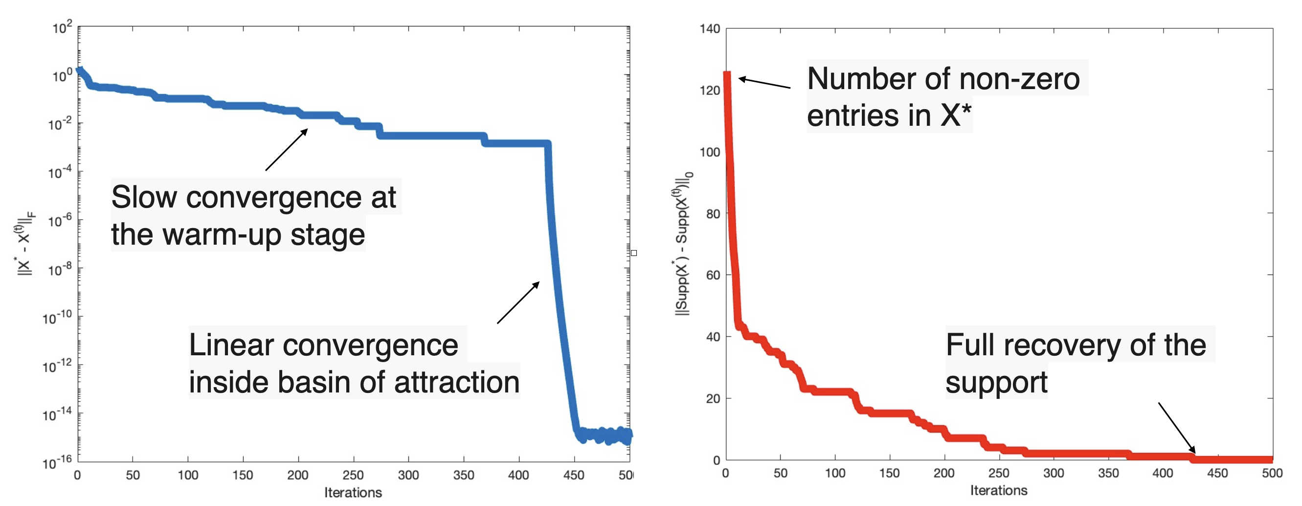
Figure 2: The plots above show a typical run of Algorithm 1 where $p=100$, $n=5$ and $\theta=0.3$. The figure on the left shows the Frobenius norm of $\bm{X}^{*}-\bm{X}^{(t)}$ per iteration. The figure on the right shows the number of non-zero entries of $\mathrm{Supp}(\bm{X}^{*})-\mathrm{Supp}(\bm{X}^{(t)})$. The number is 126 at the beginning, which is the total number of non-zero entries in $\bm{X}^{*}$, and 0 in the end, which indicates the full recovery of the support of $\bm{X}^{*}$.

3.4.2 Further Speed-up for Online Dictionary Learning

Even though Algorithm 3 works in an online setting, its computational cost is bottlenecked by the matrix-matrix multiplication and the SVD step, leading to a per-iteration cost of $O(n^{3})$. Here, we propose a possible way to further speed up the algorithm by considering $\tilde{\bm{Y}}^{(t)}\tilde{\bm{X}}^{(t)\top}$ as the sum of rank-one matrices $\tilde{\bm{y}}\tilde{\bm{x}}^{\top}$. More specifically, after receiving $\bm{y}$ at each iteration, we use $\bm{y}$ to calculate only one pair of $\tilde{\bm{y}}$ and $\tilde{\bm{x}}$ with the current preconditioner $\bm{P}^{(t)}$ and the current dictionary $\bm{D}^{(t)}$. Then we can perform rank-one update on $\mathrm{Polar}(\cdot)$ which can be performed in $O(n^{2})$ theoretically (Stange, (2008)). The per-iteration cost of $O(n^{2})$ must be optimal since it is the same cost of forming and storing an $n\times n$ dictionary. However, as delineated by Stange, (2008), the proposed rank-one update of the polar decomposition cannot be efficiently implemented in practice despite its desirable computational cost in theory. Therefore, we leave the practical implementation of this technique to future research.

4 Numerical Experiments

In this section, we evaluate the performance of our algorithm in practice. In particular, we consider the task of learning a dictionary for the Yale Face Databse , which consists of 60000 greyscale images for individual faces. Experiments in this section are performed on a MacBook Pro 2021 with the Apple M1 Pro chip and a 16GB unified memory for a serial implementation in MATLAB 2022a. Our experiments demonstrate that our method significantly outperforms KSVD in terms of running time and image reconstruction quality.

For a fair comparison, we randomly sample 1000 grey scale images and compare the learned dictionary using Algorithm 3, KSVD, and the standard discrete fourier transform. For large sample sizes, previous methods like full-batch alternating minimization and KSVD have prohibitively expensive runtimes, while the speed and convergence of our mini-batch algorithm 3 is almost unaffected, since its per-iteration cost is independent of the sample size $p$. The only reason we keep the number of training data relatively small is that KSVD is extremely slow compared to Algorithm 3 and running KSVD with 60000 greyscale images will take multiple days in our current setup. In contrast, Algorithm 3 only takes a few minutes.

Using the learned dictionary, we compare the results of two common tasks: (1) image reconstruction and (2) image denoising using the learned dictionary. In both of these tasks, we can clearly see that the dictionary learned via Algorithm 3 achieves a better reconstruction using much less time.

Image Reconstruction

A pair of the reconstruction results are shown in Figure 3. To generate this plot we randomly sample 1000 figures of individual faces of size $50\times 50$. Instead of directly learning a dictionary for the dataset, we follow the procedure in Aharon et al., (2006) and divide each figure into 25 tiles of $10\times 10$ patches. These patches are then reshaped into a $100\times 1$ vector and stacked together into a matrix $Y$ of size $100\times 25000$. This corresponds to $n=100$ and $p=25000$ in our theoretical results. Unfortunately, while such a large $p$ poses no issue for our proposed algorithm, it is prohibitive for KSVD. Therefore we sub-sample 5000 columns of $Y$, so that now $Y$ is of size $100\times 5000$. Our goal now is to learn a dictionary $A$ of size $100\times 100$ for this data matrix.

For a fair comparison, we select a termination time of 50 seconds for both algorithms. For reference, we also plot the image constructed using a discrete cosine transform (DCT), assuming the same sparsity level. Here the implementation of KSVD is done using a standard sparse learning library in Matlab (Mairal et al.,, 2007) and the discrete cosine transform is done using the Matlab function dct2.

Similar to the setting in Aharon et al., (2006), we choose a sparsity level of approximately 35%, which simply corresponds to using 35 atoms for reconstruction. With a given dictionary, the reconstruction is done using a standard implementation of orthogonal matching pursuit (OMP) found in the SPAMs library in Matlab (Mairal et al.,, 2007). In Figure 3, we see that our proposed method achieves a better reconstruction than both KSVD and DCT.

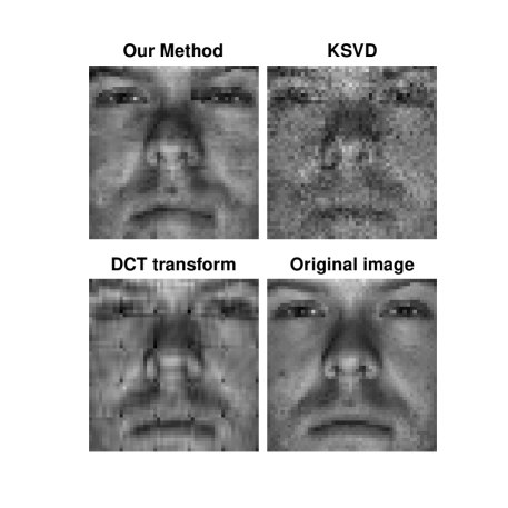
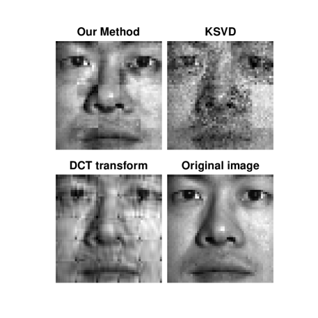
Figure 3: A comparison of image reconstruction using our proposed method (Algorithm 3), KSVD and DCT. Given a dataset of multiple greyscale images, we divided each image into patches and stack them into a large data matrix. A dictionary is learned using our minibatch alternating minimization algorithm, KSVD and DCT. For fair comparison, we cap the runtime of all algorithms at 50 seconds. Reconstruction results for two random images are shown in the upper and lower blocks. We use 35 atoms corresponding a sparsity level of 35%. We see that our method achieves a much better reconstruction than both KSVD and DCT.

Image Denoising

In addition to image reconstruction, we also gauge the quality of our learned dictionary using a common task in image processing which is called denoising. Here, an image is corrupted with 50% missing pixels (in our implementation this corresponds to setting the greyscale value to 0). Our goal is to learn a dictionary and use it to denoise this image by filling in the missing pixels. The setting in which we learn the dictionary is exactly the same as before: we divided each image into patches and stack them into a large, wide matrix. The running time for both Algorithm 3 and KSVD are capped at 50 seconds.

Once a dictionary is learned, the reconstruction is done using orthogonal matching pursuit. Here the sparsity level is the same as in the reconstruction case, i.e., 35%. A comparison of denoised results using dictionaries learned with Algorithm 3 and KSVD are shown in Figure 1. For reference, we also include results using a dictionary learned via DCT. Here we also see that the dictionary learned by Algorithm 3 outperforms both KSVD and DCT, achieving a much better reconstruction of the original image despite the fact that half of the pixels are missing.

5 Conclusion

In this paper, we study dictionary learning problem, where the goal is to represent a given set of data samples as linear combinations of a few atoms from a learned dictionary. The existing algorithms for dictionary learning often lack scalability or provable guarantees. In this paper, we show that a simple alternating minimization algorithm provably solves both orthogonal and complete dictionary learning problems. Unlike other provably convergent algorithms for dictionary learning, our proposed method does not rely on any convex relaxation of the problem, and can be easily implemented in realistic scales. Through realistic case studies on image reconstruction and image denoising, we showcase the superiority of our proposed algorithm compared with the most commonly-used algorithms for dictionary learning.

Appendix A Preliminaries

Before presenting the proofs of our main theorems, in this section we present some preliminary results in high dimensional statistics and matrix perturbation theory which will be useful in the later sections. We start with a classic result in covariance estimation for sub-Gaussian distributions. We denote the sub-Gaussian norm and $L^{2}$ norm of a random variable with $\|\cdot\|_{\psi_{2}}$ and $\|\cdot\|_{L^{2}}$ respectively.

Theorem 4 (Tail Bound for Covariance Estimation (Vershynin,, 2018)).

Let $\bm{x}$ be a sub-Gaussian random vector in $\mathbb{R}^{n}$ with covariance matrix $\bm{\Sigma}$, such that

$$\|\langle\bm{x},\bm{z}\rangle\|_{\psi_{2}}\leq C_{ce}\|\langle\bm{x},\bm{z}\rangle\|_{L^{2}}\quad\text{for any }\bm{z}\in\mathbb{R}^{n},$$ (9)

for some $C_{ce}\geq 1$. Let $\bm{X}\in\mathbb{R}^{n\times p}$ be a matrix whose columns have the identical and independent distribution as $\bm{x}$. Then, we have for any $u\geq 0$,

$$\left\|\frac{1}{p}\bm{X}\bm{X}^{\top}-\bm{\Sigma}\right\|_{2}\lesssim C_{ce}^{2}\left(\sqrt{\frac{n+u}{p}}+\frac{n+u}{p}\right)\|\bm{\Sigma}\|_{2}$$ (10)

with probability at least $1-2\exp{(-u)}$.

The next theorem describes the concentration of the norm of a random vector whose entries are sub-Gaussian random variables.

Theorem 5 (Concentration of the norm (Vershynin,, 2018)).

Let $\bm{x}=\left(\bm{x}_{1},\ldots,\bm{x}_{n}\right)\in\mathbb{R}^{n}$ be a random vector with independent, sub-Gaussian coordinates $\bm{x}_{i}$ that satisfy $\mathbb{E}\bm{x}_{i}^{2}=$ 1. Then

$$\|\|\bm{x}\left\|{}_{2}-\sqrt{n}\right\|_{\psi_{2}}\leq CK^{2},$$ (11)

where $K=\max_{i}\left\|\bm{x}_{i}\right\|_{\psi_{2}}$ and $C$ is an absolute constant.

Finally we introduce the perturbation bound for the polar factorization.

Theorem 6 (Perturbation Bound for the Unitary Polar Factor (Li,, 1995))).

Let $\bm{A}$ and $\tilde{\bm{A}}$ be two full rank $n\times n$ matrices with polar decompositions $\bm{A}=\bm{U}\bm{P}$ and $\tilde{\bm{A}}=\tilde{\bm{U}}\tilde{\bm{P}}$. Then

$$\|\bm{U}-\tilde{\bm{U}}\|_{F}\leq\frac{2}{\sigma_{n}(\bm{A})+\sigma_{n}(\tilde{\bm{A}})}\|\bm{A}-\tilde{\bm{A}}\|_{F}.$$ (12)

Appendix B Proof of Main Theorems

In this section we present the proofs of our main theorems. First, we present the proof of Theorem 1. Then, we will present the proof of Theorem 3. The proof of Theorem 2 immediately follows from the proof of Theorem 3 as a simpler case.

B.1 Proof of Theorem 1

We use induction to prove Theorem 1. The induction hypothesis we need is:

$$\|\bm{D}^{(s)}-\bm{D}^{*}\|_{F}\leq O\left(\frac{1}{\log n}\right)\qquad\text{at iteration $s$.}$$ (13)

The base case is easily verified given the initial condition. Since $\|\bm{D}^{(0)}-\bm{D}^{*}\|_{2,\infty}\leq\|\bm{D}^{(0)}-\bm{D}^{*}\|_{F}$, we can invoke the following lemma—which is a special case of (Arora et al.,, 2015, Lemma 16)—to show exact support recovery.

Lemma 1 (Exact Support Recovery for Sparse Coding).

Consider $\bm{Y}=\bm{D}^{*}\bm{X}^{*}$ where $\bm{D}^{*}\in\mathbb{O}^{n}$ and $\bm{X}^{*}$ are drawn from distributions satisfying Assumption 1. Suppose that $\bm{D}$ satisfies

$$\|\bm{D}-\bm{D}^{*}\|_{2,\infty}\leq O\left(\frac{1}{\log n}\right),$$ (14)

Then, with probability at least $1-2\exp\left\{\log(pn)-C\log^{2}n\right\}$ for some universal constant $C$, we have

$$\mathrm{supp}\left(\mathrm{HT}_{\Gamma/2}\left(\bm{D}^{\top}\bm{Y}\right)\right)=\mathrm{supp}\left(\bm{X}^{*}\right).$$ (15)

Lemma 1 together with our induction hypothesis (13) implies that

$$\mathrm{supp}\left(\bm{X}^{(s)}\right)=\mathrm{supp}\left(\bm{X}^{*}\right).$$ (16)

We use the exact recovery of support to bound the error on the sparse code:

$$\|\bm{X}^{(s)}-\bm{X}^{*}\|_{F} =\|\mathrm{HT}_{C/2}(\bm{D}^{(s)\top}\bm{Y})-\bm{X}^{*}\|_{F}$$

$$\overset{(a)}{\leq}\|\bm{D}^{(s)\top}\bm{Y}-\bm{D}^{*\top}\bm{Y}\|_{F}$$

$$\leq\|\bm{D}^{(s)}-\bm{D}^{*}\|_{F}\|\bm{Y}\|_{2},$$ (17)

where we used (16) for inequality (a). The above inequality implies that

$$\frac{\|\bm{X}^{(s)}-\bm{X}^{*}\|_{F}}{\|\bm{X}^{*}\|_{2}} =\frac{\|\bm{X}^{(s)}-\bm{X}^{*}\|_{F}}{\|\bm{D}^{*}\bm{X}^{*}\|_{2}}$$

$$=\frac{\|\bm{X}^{(s)}-\bm{X}^{*}\|_{F}}{\|\bm{Y}\|_{2}}$$

$$\leq\|\bm{D}^{(s)}-\bm{D}^{*}\|_{F}$$

$$\leq O\left(\frac{1}{\log n}\right)$$ (18)

To proceed, we need the following lemma, the proof of which can be found in Appendix C.

Lemma 2 (Guaranteed Improvement on Polar Decomposition).

Suppose $\bm{X}^{*}$ is drawn from distribution satisfying Assumption 1, $\bm{Y}=\bm{D}^{*}\bm{X}^{*}$, $p\geq\Omega(n/\theta^{2})$, and we have an approximation $\bm{X}$ of $\bm{X}^{*}$ such that $\frac{\|\bm{X}-\bm{X}^{*}\|_{F}}{\|\bm{X}^{*}\|_{2}}\leq O(\sqrt{\theta})$, then with high probability we have

$$\|\mathrm{Polar}(\bm{Y}\bm{X}^{\top})-\bm{D}^{*}\|_{F}<\frac{6\sqrt{\theta}\|\bm{X}-\bm{X}^{*}\|_{F}}{\|\bm{X}^{*}\|_{2}}.$$ (19)

Invoking Lemma 2 with $\bm{X}=\bm{X}^{(s)}$ together with (B.1) leads to

$$\|\bm{D}^{(s+1)}-\bm{D}^{*}\|_{F}<\frac{6\sqrt{\theta}\|\bm{X}^{(s)}-\bm{X}^{*}\|_{F}}{\|\bm{X}^{*}\|_{2}}.$$ (20)

As a result, we successfully show that for $\theta<1/144$, we have

$$\|\bm{D}^{(s+1)}-\bm{D}^{*}\|_{F}<\frac{\|\bm{X}^{(s)}-\bm{X}^{*}\|_{F}}{2\|\bm{X}^{*}\|_{2}}\leq\frac{1}{2}\|\bm{D}^{(s)}-\bm{D}^{*}\|_{F}.$$ (21)

Therefore, the induction hypothesis (13) holds for $t=s+1$. Consequently, the linear convergence for $\frac{\|\bm{X}^{(s)}-\bm{X}^{*}\|_{F}}{\|\bm{X}^{*}\|_{2}}$ follows from (B.1) and (21):

$$\frac{\|\bm{X}^{(s+1)}-\bm{X}^{*}\|_{F}}{\|\bm{X}^{*}\|_{2}} \leq\|\bm{D}^{(s+1)}-\bm{D}^{*}\|_{F}<\frac{\|\bm{X}^{(s)}-\bm{X}^{*}\|_{F}}{2\|\bm{X}^{*}\|_{2}}.$$

This completes the proof.$\hfill\square$

B.2 Proof of Theorem 3

The linear convergence of $\bm{A}^{(t)}$ hinges on the linear convergence of $\bm{D}^{(t)}$ towards

$$\bm{D}^{*}=\mathcal{L}((\bm{A}^{*}\bm{A}^{*\top})^{-1})^{\top}\bm{A}^{*}.$$ (22)

Specifically, the main challenge in the proof is to show the following linear convergence:

$$\|\bm{D}^{(s+1)}-\bm{D}^{*}\|_{F}\leq\rho\|\bm{D}^{(s)}-\bm{D}^{*}\|_{F}+O\left(\|\bm{P}^{(s)}\bm{A}^{*}-\bm{D}^{*}\|_{F}\right),$$ (23)

for some $0<\rho<1$. To this goal, we introduce the following intermediate lemmas, the proofs of which can be found in Appendix C.

Lemma 3 (Preconditioner Approximation).

Under Assumption 1, with high probability we have:

$$\left\|\bm{P}^{(t)}-\mathcal{L}\left(\left(\bm{A}^{*}\bm{A}^{*\top}\right)^{-1}\right)^{\top}\right\|_{2}\leq O\left(\frac{\hat{\kappa}^{6}}{\theta}\sqrt{\frac{n}{p_{1}+t}}\right).$$ (24)

Lemma 4 (Spectral Property for Sparse Code Matrix).

For a random matrix $\bm{X}$ that is drawn from distribution satisfying Assumption 1 and $p\geq\Omega(n/\theta^{2})$, we have

$$\|\bm{X}\|_{2}\leq\frac{11}{10} \sqrt{p\theta}\sigma,\quad\sigma_{n}\left(\bm{X}\right)\geq\frac{9}{10}\sqrt{p\theta}\sigma,\quad\kappa\left(\bm{X}\right)\leq\frac{11}{9},$$ (25)

with high probability.

For the remainder of this section, we abuse the notation and use $\bm{X}^{*}$ to denote the sparse coding matrix that generates $\bm{Y}^{(s)}=\bm{A}^{*}\bm{X}^{*}$, where $\bm{Y}^{(s)}$ is obtained by adding the latest sample as the last column and removing the oldest sample from its first column (see Steps 6 and 7 in Algorithm 3). Indeed, $\bm{X}^{*}$ is different from iteration to iteration, but it plays a similar role in the proof to the ground truth matrix in the full-batch case. We also consider $\tilde{\bm{X}}$ to be $\tilde{\bm{X}}=\bm{D}^{*\top}\tilde{\bm{Y}}^{(s)}$, which is again a different sparse coding matrix for different iterations since $\tilde{\bm{Y}}^{(s)}=\bm{P}^{(s)}\bm{Y}^{(s)}$ and both $\bm{P}^{(s)}$ and $\bm{Y}^{(s)}$ change from iteration to iteration.

Towards proving (23), we first show that $\tilde{\bm{X}}^{(s)}$ recovers the sparsity pattern of $\bm{X}^{*}$ if we use enough number of samples to construct the preconditioner. We consider one entry $\left(\bm{D}^{(s)\top}\tilde{\bm{Y}}^{(s)}\right)_{ij}$ of $\bm{D}^{(s)\top}\tilde{\bm{Y}}^{(s)}$ and write

$$\left(\bm{D}^{(s)\top}\tilde{\bm{Y}}^{(s)}\right)_{ij}= \left(\bm{D}^{(s)\top}\bm{D}^{*}\tilde{\bm{X}}\right)_{ij}$$

$$= \left(\bm{D}^{(s)\top}\bm{D}^{*}(\tilde{\bm{X}}-\bm{X}^{*})\right)_{ij}+\left(\bm{D}^{(s)\top}\bm{D}^{*}\bm{X}^{*}\right)_{ij}.$$ (26)

The first term can be bounded as

$$\left|\left(\bm{D}^{(s)\top}\bm{D}^{*}(\tilde{\bm{X}}-\bm{X}^{*})\right)_{ij}\right|\leq\ \|\bm{D}^{(s)\top}\bm{D}^{*}\|_{2}\|\tilde{\bm{X}}-\bm{X}^{*}\|_{2,\inf}$$

$$=\ \|\tilde{\bm{X}}-\bm{X}^{*}\|_{2,\inf}$$

$$\leq\ \|\bm{D}^{*\top}\bm{P}^{(s)}\bm{A}^{*}\bm{X}^{*}-\bm{X}^{*}\|_{2,\inf}$$

$$\leq\ \|\bm{P}^{(s)}\bm{A}^{*}-\bm{D}^{*}\|_{2}\|\bm{X}^{*}\|_{2,\inf}$$

$$\leq\ \left\|\bm{P}^{(s)}-\mathcal{L}\left(\left(\bm{A}^{*}\bm{A}^{*\top}\right)^{-1}\right)\right\|_{2}\|\bm{A}^{*}\|_{2}\|\bm{X}^{*}\|_{2,\inf}$$

$$\lesssim\ \frac{\hat{\kappa}^{6}}{\theta}\sqrt{\frac{n}{p_{1}+t}}\|\bm{X}^{*}\|_{2,\inf}.$$ (27)

The last inequality is a result of Lemma 3. As will be clear in its proof, Lemma 3 holds with probability of at least $1-2\exp(-\log^{2}n)$, which allows us to invoke it for every $\bm{P}^{(s)}$. The term $\|\bm{X}^{*}\|_{2,\inf}$ denotes the largest column norm of matrix $\bm{X}^{*}$. The expectation for the norm of each column, based on Assumption 1, is $\sigma\sqrt{\theta n}$. The random variable $\|\bm{X}^{*}_{(\cdot,k)}\|_{2}-\sigma\sqrt{\theta n}$ is sub-Gaussian with sub-Gaussian norm $O(\sqrt{\theta}\sigma)$ by Theorem 5. As a result, we can bound the norm of the $k$th column of $\bm{X}^{*}$ as

$$\mathbb{P}\left(\|\bm{X}^{*}_{(\cdot,k)}\|_{2}\geq 2\sigma\sqrt{\theta n}\right)\leq 2\exp\left(-Cn\right),$$ (28)

for some constant $C$. After taking the union bound, we have

$$\|\bm{X}^{*}\|_{2,\inf}=\max_{1\leq k\leq p_{2}}\|\bm{X}_{(\cdot,k)}^{*}\|_{2}\leq 2\sigma\sqrt{\theta n\log p_{2}}$$ (29)

with probability of at least $1-2T\exp\left(-Cn\right)$. Therefore, we have that with high probability,

$$\left|\left(\bm{D}^{(s)\top}\bm{D}^{*}(\tilde{\bm{X}}-\bm{X}^{*})\right)_{ij}\right|\lesssim\frac{\hat{\kappa}^{6}\sigma}{\sqrt{\theta}}\sqrt{\frac{n^{2}\log p_{2}}{p_{1}+t}},$$ (30)

for every $(i,j)$. Based on the above inequality and with the choice of $p_{1}\geq\Omega(n^{2}\log n\sigma^{2}\hat{\kappa}^{12}/(\theta^{2}\Gamma))$, we have $\left|\left(\bm{D}^{(s)\top}\bm{D}^{*}(\tilde{\bm{X}}-\bm{X}^{*})\right)_{ij}\right|<\Gamma/4$. Now, recalling (B.2), we have bounded the first term by $\Gamma/4$. The deviation of the second term from $X^{*}_{ij}$ can also be bounded by $\Gamma/4$ with high probability, by the proof of Lemma 1 which will not be repeated here. To sum up, we have $|\left(\bm{D}^{(s)\top}\tilde{\bm{Y}}^{(s)}\right)_{ij}|<\Gamma/2$ when $X^{*}_{ij}=0$ and $|\left(\bm{D}^{(s)\top}\tilde{\bm{Y}}^{(s)}\right)_{ij}|>\Gamma/2$ when $X^{*}_{ij}\neq 0$, which leads to

$$\mathrm{supp}\left(\tilde{\bm{X}}^{(s)}\right)=\mathrm{supp}(\bm{X}^{*}).$$ (31)

From now on, we use $\mathcal{P}(\cdot)$ to denote a projection of a matrix onto $\mathrm{supp}(\bm{X}^{*})$. Specifically, for any matrix $\bm{A}\in\mathbb{R}^{n\times p_{2}}$, we have

$$\left(\mathcal{P}(\bm{A})\right)_{ij}=\begin{cases}\bm{A}_{ij}&\text{if}\quad(i,j)\in\mathrm{supp}(\bm{X}^{*})\\ 0&\text{if}\quad(i,j)\not\in\mathrm{supp}(\bm{X}^{*})\end{cases}.$$ (32)

Given the exact support recovery, we have

$$\|\tilde{\bm{X}}^{(s)}-\mathcal{P}(\tilde{\bm{X}})\|_{F} =\|\mathcal{P}(\bm{D}^{(s)\top}\tilde{\bm{Y}}^{(s)})-\mathcal{P}(\tilde{\bm{X}})\|_{F}$$

$$\leq\|\bm{D}^{(s)\top}\tilde{\bm{Y}}^{(s)}-\tilde{\bm{X}}\|_{F}$$

$$=\|\bm{D}^{(s)\top}\tilde{\bm{Y}}^{(s)}-\bm{D}^{*\top}\tilde{\bm{Y}}^{(s)}\|_{F}$$

$$\leq\|\bm{D}^{(s)}-\bm{D}^{*}\|_{F}\|\tilde{\bm{Y}}^{(s)}\|_{2}$$

$$=\|\bm{D}^{(s)}-\bm{D}^{*}\|_{F}\|\tilde{\bm{X}}\|_{2}.$$ (33)

As a result we have

$$\frac{\|\tilde{\bm{X}}^{(s)}-\mathcal{P}(\tilde{\bm{X}})\|_{F}}{\|\mathcal{P}(\tilde{\bm{X}})\|_{2}}$$

$$=\ \frac{\|\tilde{\bm{X}}^{(s)}-\mathcal{P}(\tilde{\bm{X}})\|_{F}}{\|\tilde{\bm{X}}\|_{2}}\frac{\|\tilde{\bm{X}}\|_{2}}{\|\mathcal{P}(\tilde{\bm{X}})\|_{2}}$$

$$\leq\ \|\bm{D}^{(s)}-\bm{D}^{*}\|_{F}\frac{\|\tilde{\bm{X}}\|_{2}}{\|\tilde{\bm{X}}\|_{2}-\|\tilde{\bm{X}}-\mathcal{P}(\tilde{\bm{X}})\|_{2}}$$

$$\leq\ \|\bm{D}^{(s)}-\bm{D}^{*}\|_{F}\frac{\|\tilde{\bm{X}}\|_{2}}{\|\tilde{\bm{X}}\|_{2}-\|\tilde{\bm{X}}-\mathcal{P}(\tilde{\bm{X}})\|_{F}}$$

$$\overset{(a)}{\leq}\ \|\bm{D}^{(s)}-\bm{D}^{*}\|_{F}\frac{\|\tilde{\bm{X}}\|_{2}}{\|\tilde{\bm{X}}\|_{2}-\|\tilde{\bm{X}}-\bm{X}^{*}\|_{F}}$$

$$\overset{(b)}{\leq}\ \|\bm{D}^{(s)}-\bm{D}^{*}\|_{F}\left(1+\frac{\|\tilde{\bm{X}}-\bm{X}^{*}\|_{F}}{\|\bm{X}^{*}\|_{2}-2\|\tilde{\bm{X}}-\bm{X}^{*}\|_{F}}\right)$$

$$\leq\ \|\bm{D}^{(s)}-\bm{D}^{*}\|_{F}\left(1+\frac{\frac{\|\tilde{\bm{X}}-\bm{X}^{*}\|_{F}}{\|\bm{X}^{*}\|_{2}}}{1-\frac{2\|\tilde{\bm{X}}-\bm{X}^{*}\|_{F}}{\|\bm{X}^{*}\|_{2}}}\right)$$

$$\overset{(c)}{\leq}\ \|\bm{D}^{(s)}-\bm{D}^{*}\|_{F}\left(1+\frac{\frac{1}{10}}{1-2\times\frac{1}{10}}\right)$$

$$=\ \frac{9}{8}\|\bm{D}^{(s)}-\bm{D}^{*}\|_{F}.$$ (34)

Here inequality (a) is due to the decomposition of $\tilde{\bm{X}}-\bm{X}^{*}$ onto and outside the support of $\bm{X}^{*}$. Specifically, consider $\mathcal{P}_{\perp}(\cdot)$ to be the projection orthogonal to $\bm{P}(\cdot)$. We have $\mathcal{P}_{\perp}(\tilde{\bm{X}}-\mathcal{P}(\tilde{\bm{X}}))=\mathcal{P}_{\perp}(\tilde{\bm{X}}-\bm{X}^{*})$ while $\mathcal{P}(\tilde{\bm{X}}-\mathcal{P}(\tilde{\bm{X}}))$ is an all zero matrix. So we can conclude $\|\tilde{\bm{X}}-\mathcal{P}(\tilde{\bm{X}})\|_{F}\leq\|\tilde{\bm{X}}-\bm{X}^{*}\|_{F}$. The inequality (b) is from $\|\bm{X}^{*}\|_{2}-\|\tilde{\bm{X}}-\bm{X}^{*}\|_{F}\leq\|\bm{X}^{*}\|_{2}-\|\tilde{\bm{X}}-\bm{X}^{*}\|_{2}\leq\|\tilde{\bm{X}}\|_{2}$. The inequality (c) holds due to $\frac{\|\tilde{\bm{X}}-\bm{X}^{*}\|_{F}}{\|\bm{X}^{*}\|_{2}}\leq 1/10$, which is a result from Lemma 3:

$$\|\tilde{\bm{X}}-\bm{X}^{*}\|_{F} =\|\bm{D}^{*\top}\bm{P}^{(s)}\bm{A}^{*}\bm{X}^{*}-\bm{X}^{*}\|_{F}$$

$$\leq\|\bm{P}^{(s)}\bm{A}^{*}-\bm{D}^{*}\|_{F}\|\bm{X}^{*}\|_{2}$$

$$\leq\sqrt{n}\|\bm{P}^{(s)}\bm{A}^{*}-\bm{D}^{*}\|_{2}\|\bm{X}^{*}\|_{2}$$

$$\lesssim\frac{\hat{\kappa}^{6}}{\theta}\sqrt{\frac{n^{2}}{p_{1}+t}}\|\bm{X}^{*}\|_{2},$$ (35)

and $p_{1}\geq\Omega(n^{2}\log n\sigma^{2}\hat{\kappa}^{12}/(\theta^{2}\Gamma))$.

So far, we have bounded $\frac{\|\tilde{\bm{X}}^{(s)}-\mathcal{P}(\tilde{\bm{X}})\|_{F}}{\|\mathcal{P}(\tilde{\bm{X}})\|_{2}}$ with $\|\bm{D}^{(s)}-\bm{D}^{*}\|_{F}$, the next step is to bound $\|\bm{D}^{(s+1)}-\bm{D}^{*}\|_{F}$ with $\frac{\|\tilde{\bm{X}}^{(s)}-\mathcal{P}(\tilde{\bm{X}})\|_{F}}{\|\mathcal{P}(\tilde{\bm{X}})\|_{2}}$. For $\|\bm{D}^{(s+1)}-\bm{D}^{*}\|_{F}$, we have

$$\|\bm{D}^{(s+1)}-\bm{D}^{*}\|_{F}$$

$$=\ \|\mathrm{Polar}(\tilde{\bm{Y}}^{(s)}\tilde{\bm{X}}^{(s)\top})-\bm{D}^{*}\|_{F}$$

$$=\ \|\mathrm{Polar}(\bm{D}^{*}\tilde{\bm{X}}\tilde{\bm{X}}^{(s)\top})-\bm{D}^{*}\|_{F}$$

$$=\ \|\mathrm{Polar}(\bm{D}^{*}\tilde{\bm{X}}\tilde{\bm{X}}^{(s)\top})-\mathrm{Polar}(\bm{D}^{*}\mathcal{P}(\tilde{\bm{X}})\tilde{\bm{X}}^{(s)\top})$$

$$+\mathrm{Polar}(\bm{D}^{*}\mathcal{P}(\tilde{\bm{X}})\tilde{\bm{X}}^{(s)\top})-\bm{D}^{*}\|_{F}$$

$$=\ \|\mathrm{Polar}(\bm{D}^{*}\tilde{\bm{X}}\tilde{\bm{X}}^{(s)\top})-\mathrm{Polar}(\bm{D}^{*}\mathcal{P}(\tilde{\bm{X}})\tilde{\bm{X}}^{(s)\top})\|_{F}$$

$$+\|\mathrm{Polar}(\bm{D}^{*}\mathcal{P}(\tilde{\bm{X}})\tilde{\bm{X}}^{(s)\top})-\bm{D}^{*}\|_{F}$$ (36)

To bound the first term $\|\mathrm{Polar}(\bm{D}^{*}\tilde{\bm{X}}\tilde{\bm{X}}^{(s)\top})-\mathrm{Polar}(\bm{D}^{*}\mathcal{P}(\tilde{\bm{X}})\tilde{\bm{X}}^{(s)\top})\|_{F}$, we invoke Theorem 6 and get

$$\|\mathrm{Polar}(\bm{D}^{*}\tilde{\bm{X}}\tilde{\bm{X}}^{(s)\top})-\mathrm{Polar}(\bm{D}^{*}\mathcal{P}(\tilde{\bm{X}})\tilde{\bm{X}}^{(s)\top})\|_{F}$$

$$\leq\ \frac{2\|\bm{D}^{*}\tilde{\bm{X}}\tilde{\bm{X}}^{(s)\top}-\bm{D}^{*}\mathcal{P}(\tilde{\bm{X}})\tilde{\bm{X}}^{(s)\top}\|_{F}}{\sigma_{n}(\bm{D}^{*}\tilde{\bm{X}}\tilde{\bm{X}}^{(s)\top})+\sigma_{n}(\bm{D}^{*}\mathcal{P}(\tilde{\bm{X}})\tilde{\bm{X}}^{(s)\top})}$$

$$\overset{(a)}{\leq}\ \frac{2\kappa(\tilde{\bm{X}}^{(s)})\|\tilde{\bm{X}}-\mathcal{P}(\tilde{\bm{X}})\|_{F}}{2\sigma_{n}(\bm{X}^{*})-\|\bm{X}^{*}-\tilde{\bm{X}}\|_{2}-\|\bm{X}^{*}-\mathcal{P}(\tilde{\bm{X}})\|_{2}}$$

$$=\ \frac{2\kappa(\tilde{\bm{X}}^{(s)})\|\tilde{\bm{X}}-\mathcal{P}(\tilde{\bm{X}})\|_{F}}{\|\bm{X}^{*}\|_{2}}\cdot\frac{1}{\frac{2}{\kappa(\bm{X}^{*})}-\frac{\|\bm{X}^{*}-\tilde{\bm{X}}\|_{2}}{\|\bm{X}^{*}\|_{2}}-\frac{\|\bm{X}^{*}-\mathcal{P}(\tilde{\bm{X}})\|_{2}}{\|\bm{X}^{*}\|_{2}}}$$

$$\overset{(b)}{\leq}\ \frac{2\kappa(\tilde{\bm{X}}^{(s)})\|\tilde{\bm{X}}-\mathcal{P}(\tilde{\bm{X}})\|_{F}}{\|\bm{X}^{*}\|_{2}}\frac{1}{18/11-1/10-1/10}$$

$$\leq\ \frac{3\kappa(\tilde{\bm{X}}^{(s)})\|\tilde{\bm{X}}-\mathcal{P}(\tilde{\bm{X}})\|_{F}}{\|\bm{X}^{*}\|_{2}}$$ (37)

Inequality (a) is due to normalizing both the numerator and the denominator with $\|\tilde{\bm{X}}^{(s)}\|_{2}$. In inequality (b) we use the result of Lemma 4. Next we aim to find a bound on $\kappa(\tilde{\bm{X}}^{(s)})$, and we do so by first bounding $\kappa(\mathcal{P}(\tilde{\bm{X}}))$. By Lemma 4 and Lemma 3, we have

$$\kappa(\mathcal{P}(\tilde{\bm{X}})) =\frac{\|\mathcal{P}(\tilde{\bm{X}})\|_{2}}{\sigma_{n}(\mathcal{P}(\tilde{\bm{X}}))}$$

$$\leq\frac{\|\bm{X}^{*}\|_{2}+\|\mathcal{P}(\tilde{\bm{X}})-\bm{X}^{*}\|_{2}}{\sigma_{n}(\bm{X}^{*})-\|\mathcal{P}(\tilde{\bm{X}})-\bm{X}^{*}\|_{2}}$$

$$=\frac{\|\bm{X}^{*}\|_{2}+\|\mathcal{P}(\tilde{\bm{X}})-\bm{X}^{*}\|_{2}}{\|\bm{X}^{*}\|_{2}/\kappa(\bm{X}^{*})-\|\mathcal{P}(\tilde{\bm{X}})-\bm{X}^{*}\|_{2}}$$

$$\leq\frac{1+\|\mathcal{P}(\tilde{\bm{X}})-\bm{X}^{*}\|_{F}/\|\bm{X}^{*}\|_{2}}{1/\kappa(\bm{X}^{*})-\|\mathcal{P}(\tilde{\bm{X}})-\bm{X}^{*}\|_{F}/\|\bm{X}^{*}\|_{2}}$$

$$\leq\frac{1+1/10}{9/11-1/10}$$

$$=\frac{121}{79}.$$ (38)

By a similar argument we have

$$\kappa(\tilde{\bm{X}}^{(s)}) \leq\frac{\|\mathcal{P}(\tilde{\bm{X}})\|_{2}+\|\mathcal{P}(\tilde{\bm{X}})-\tilde{\bm{X}}^{(s)}\|_{2}}{\sigma_{n}(\mathcal{P}(\tilde{\bm{X}}))-\|\mathcal{P}(\tilde{\bm{X}})-\tilde{\bm{X}}^{(s)}\|_{2}}$$

$$\leq\frac{1+\|\mathcal{P}(\tilde{\bm{X}})-\tilde{\bm{X}}^{(s)}\|_{F}/\|\mathcal{P}(\tilde{\bm{X}})\|_{2}}{1/\kappa(\mathcal{P}(\tilde{\bm{X}}))-\|\mathcal{P}(\tilde{\bm{X}})-\tilde{\bm{X}}^{(s)}\|_{F}/\|\mathcal{P}(\tilde{\bm{X}})\|_{2}}$$

$$\overset{(a)}{\leq}\frac{1+9/32}{79/121-9/32}$$

$$<4.$$ (39)

For inequality (a) we used (B.2) and the fact that $\|\bm{D}^{(s)}-\bm{D}^{*}\|_{F}\leq O(\frac{1}{\log n})\leq 1/4$. To conclude we have the first term of the right hand side of (B.2) bounded as

$$\|\mathrm{Polar}(\bm{D}^{*}\tilde{\bm{X}}\tilde{\bm{X}}^{(s)\top})-\mathrm{Polar}(\bm{D}^{*}\mathcal{P}(\tilde{\bm{X}})\tilde{\bm{X}}^{(s)\top})\|_{F} <\frac{12\|\tilde{\bm{X}}-\mathcal{P}(\tilde{\bm{X}})\|_{F}}{\|\bm{X}^{*}\|_{2}}$$

$$\leq\frac{12\|\bm{X}^{*}-\mathcal{P}(\tilde{\bm{X}})\|_{F}}{\|\bm{X}^{*}\|_{2}}.$$ (40)

Now we turn our focus to bounding the second term of (B.2), which is $\|\mathrm{Polar}(\bm{D}^{*}\mathcal{P}(\tilde{\bm{X}})\tilde{\bm{X}}^{(s)\top})-\bm{D}^{*}\|_{F}$. We first introduce the following lemma by Ravishankar et al., (2020):

Lemma 5.

For any matrix $\bm{X}^{*}\in\mathbb{R}^{n\times p}$ and $\bm{Y}=\bm{D}^{*}\bm{X}^{*}$ where $\bm{D}^{*}\in\mathbb{O}^{n}$, consider an approximation $\bm{X}$ to $\bm{X}^{*}$ such that the normalized error matrix $\bm{E}:=\left(\bm{X}-\bm{X}^{*}\right)/\|\bm{X}^{*}\|_{2}$ satisfies:

$$\|\bm{E}\|_{F}<\frac{1}{\kappa^{2}\left(\bm{X}^{*}\right)}.$$ (41)

Then an approximation to $\bm{D}^{*}$, obtained by $\bm{D}=\mathrm{Polar}(\bm{Y}\bm{X}^{\top})$, satisfies:

$$\|\bm{D}-\bm{D}^{*}\|_{F}\leq \frac{\kappa(\bm{X}^{*})^{4}}{2}\frac{\left\|\bm{X}^{*}\bm{E}^{\top}-\bm{E}\bm{X}^{*\top}\right\|_{F}}{\|\bm{X}^{*}\|_{2}}+O(\|\bm{E}\|^{2}_{F}).$$ (42)

Now we can set

$$\tilde{\bm{E}}^{(s)}=\frac{\tilde{\bm{X}}^{(s)}-\mathcal{P}(\tilde{\bm{X}})}{\|\mathcal{P}(\tilde{\bm{X}})\|_{2}},$$ (43)

and notice that

$$\|\tilde{\bm{E}}^{(s)}\|_{F} \overset{Eq~{}\ref{eq: sparse code bounded by dic complete offline}}{\leq}\frac{9}{8}\|\bm{D}^{(s)}-\bm{D}^{*}\|_{F}\leq O(1/\log n)\leq\left(\frac{79}{121}\right)^{2}\overset{Eq~{}\ref{eq: kappa P tilde X complete offline}}{\leq}\frac{1}{\kappa^{2}(\mathcal{P}(\tilde{\bm{X}}))}.$$ (44)

Upon invoking Lemma 5 we get

$$\|\mathrm{Polar}(\bm{D}^{*}\mathcal{P}(\tilde{\bm{X}})\tilde{\bm{X}}^{(s)\top})-\bm{D}^{*}\|_{F}\leq\ \frac{\kappa(\mathcal{P}(\tilde{\bm{X}}))^{4}}{2}\frac{\left\|\mathcal{P}(\tilde{\bm{X}})\tilde{\bm{E}}^{(s)\top}-\tilde{\bm{E}}^{(s)}\mathcal{P}(\tilde{\bm{X}})^{\top}\right\|_{F}}{\|\mathcal{P}(\tilde{\bm{X}})\|_{2}}+O(\|\tilde{\bm{E}}^{(s)}\|^{2}_{F}).$$ (45)

By recalling that $\mathrm{supp}(\tilde{\bm{X}}^{(s)})=\mathrm{supp}(\bm{X}^{*})$, we follow the same argument in the proof of Lemma 2 and conclude that

$$\frac{\left\|\mathcal{P}(\tilde{\bm{X}})\tilde{\bm{E}}^{(s)\top}-\tilde{\bm{E}}^{(s)}\mathcal{P}(\tilde{\bm{X}})^{\top}\right\|_{F}}{2\|\mathcal{P}(\tilde{\bm{X}})\|_{2}}\leq\frac{\max_{1\leq k\leq n}\left\|\bm{M}_{k}\mathcal{P}(\tilde{\bm{X}})\tilde{\bm{M}}_{k}\right\|_{2}\|\tilde{\bm{E}}^{(s)}\|_{F}}{\|\mathcal{P}(\tilde{\bm{X}})\|_{2}},$$ (46)

where $\bm{M}_{k}$ and $\tilde{\bm{M}}_{k}$ are defined in the same way as in the proof of Lemma 2. Since both $\bm{M}_{k}$ and $\tilde{\bm{M}}_{k}$ are linear operators, we have

$$\ \frac{\max_{1\leq k\leq n}\left\|\bm{M}_{k}\mathcal{P}(\tilde{\bm{X}})\tilde{\bm{M}}_{k}\right\|_{2}}{\|\mathcal{P}(\tilde{\bm{X}})\|_{2}}\leq \ \frac{\max_{1\leq k\leq n}\left\|\bm{M}_{k}\bm{X}^{*}\tilde{\bm{M}}_{k}\right\|_{2}+\|\mathcal{P}(\tilde{\bm{X}})-\bm{X}^{*}\|_{2}}{\|\bm{X}^{*}\|_{2}-\|\mathcal{P}(\tilde{\bm{X}})-\bm{X}^{*}\|_{2}}$$

$$\leq \ \frac{\max_{1\leq k\leq n}\left\|\bm{M}_{k}\bm{X}^{*}\tilde{\bm{M}}_{k}\right\|_{2}+\|\mathcal{P}(\tilde{\bm{X}})-\bm{X}^{*}\|_{2}}{\|\bm{X}^{*}\|_{2}(1-\|\mathcal{P}(\tilde{\bm{X}})-\bm{X}^{*}\|_{F}/\|\bm{X}^{*}\|_{2})}$$

$$\leq \ \frac{10}{9}\left(\frac{\max_{1\leq k\leq n}\left\|\bm{M}_{k}\bm{X}^{*}\tilde{\bm{M}}_{k}\right\|_{2}+\|\mathcal{P}(\tilde{\bm{X}})-\bm{X}^{*}\|_{2}}{\|\bm{X}^{*}\|_{2}}\right)$$

$$\leq \ \frac{10}{9}\left(\frac{\max_{1\leq k\leq n}\left\|\bm{M}_{k}\bm{X}^{*}\tilde{\bm{M}}_{k}\right\|_{2}}{\|\bm{X}^{*}\|_{2}}+\frac{\|\mathcal{P}(\tilde{\bm{X}})-\bm{X}^{*}\|_{F}}{\|\bm{X}^{*}\|_{2}}\right)$$

$$\leq \ \frac{10}{9}\left(\frac{\max_{1\leq k\leq n}\left\|\bm{M}_{k}\bm{X}^{*}\tilde{\bm{M}}_{k}\right\|_{2}}{\|\bm{X}^{*}\|_{2}}+\frac{1}{10}\right)$$ (47)

In the proof of Lemma 2, we have that with probability $1-2\exp(\log n-\log^{2}n)$ and the condition $p_{2}\geq\Omega(n/\theta^{2})$,

$$\frac{\max_{1\leq k\leq n}\left\|\bm{M}_{k}\bm{X}^{*}\tilde{\bm{M}}_{k}\right\|_{2}}{\|\bm{X}^{*}\|_{2}}\leq\frac{11}{9}\sqrt{\theta}.$$ (48)

Combined with (45), we have

$$\|\mathrm{Polar}(\bm{D}^{*}\mathcal{P}(\tilde{\bm{X}})\tilde{\bm{X}}^{(s)\top})-\bm{D}^{*}\|_{F}\leq \frac{\kappa(\mathcal{P}(\tilde{\bm{X}}))^{4}}{2}\frac{\left\|\mathcal{P}(\tilde{\bm{X}})\tilde{\bm{E}}^{(s)\top}-\tilde{\bm{E}}^{(s)}\mathcal{P}(\tilde{\bm{X}})^{\top}\right\|_{F}}{\|\mathcal{P}(\tilde{\bm{X}})\|_{2}}+O(\|\tilde{\bm{E}}^{(s)}\|^{2}_{F})$$

$$\leq (\frac{10}{9}\left(\frac{11}{9}\sqrt{\theta}+\frac{1}{10}\right)\kappa(\mathcal{P}(\tilde{\bm{X}}))^{4}+O(\|\tilde{\bm{E}}^{(s)}\|_{F}))\|\tilde{\bm{E}}^{(s)}\|_{F}$$ (49)

The above inequality combined with $\kappa(\mathcal{P}(\tilde{\bm{X}}))\leq 121/79$ (due to (B.2)), $\theta<1/5600$, and $\|\tilde{\bm{E}}^{(s)}\|_{F}\leq O({1}/{\log n})$ leads to

$$\|\mathrm{Polar}(\bm{D}^{*}\mathcal{P}(\tilde{\bm{X}})\tilde{\bm{X}}^{(s)\top})-\bm{D}^{*}\|_{F}\leq\frac{41}{50}\|\tilde{\bm{E}}^{(s)}\|_{F},$$ (50)

with probability of at least $1-2\exp(\log n-\log^{2}n)$. Therefore, we have a bound for the second term of (B.2). As a result, (B.2) can be rewritten as

$$\|\bm{D}^{(s+1)}-\bm{D}^{*}\|_{F}\leq\ \frac{41}{50}\|\tilde{\bm{E}}^{(s)}\|_{F}+\frac{12\|\bm{X}^{*}-\mathcal{P}(\tilde{\bm{X}})\|_{F}}{\|\bm{X}^{*}\|_{2}}$$

$$\overset{\text{Eq}\ref{eq: sparse code bounded by dic complete offline}}{\leq}\ \frac{369}{400}\|\bm{D}^{(s)}-\bm{D}^{*}\|_{F}+\frac{12\|\bm{X}^{*}-\mathcal{P}(\tilde{\bm{X}})\|_{F}}{\|\bm{X}^{*}\|_{2}}$$

$$\leq\ \frac{369}{400}\|\bm{D}^{(s)}-\bm{D}^{*}\|_{F}+12\|\bm{P}^{(s)}\bm{A}^{*}-\bm{D}^{*}\|_{F}$$ (51)

This completes the proof of the induction step (23). Finally, we use (B.2) to complete the proof of Theorem 3. This goal, notice that

$$\|\bm{A}^{(s+1)}-\bm{A}^{*}\|_{F}=\ \|\bm{P}^{(s+1)-1}\bm{D}^{(s+1)}-\left(\mathcal{L}((\bm{A}^{*}\bm{A}^{*\top})^{-1})^{\top}\right)^{-1}\bm{D}^{*}\|_{F}$$

$$\leq\ \|\bm{D}^{(s+1)}-\bm{D}^{*}\|_{F}+\|\bm{P}^{(s+1)-1}-\left(\mathcal{L}((\bm{A}^{*}\bm{A}^{*\top})^{-1})^{\top}\right)^{-1}\|_{F}$$

$$\leq\ \|\bm{D}^{(s+1)}-\bm{D}^{*}\|_{F}+O\left(\|\bm{P}^{(s+1)}-\mathcal{L}\left(\left(\bm{A}^{*}\bm{A}^{*\top}\right)^{-1}\right)^{\top}\|_{F}\right).$$ (52)

Via a similar argument, we can write

$$\|\bm{D}^{(s)}-\bm{D}^{*}\|_{F}\leq\ \|\bm{A}^{(s)}-\bm{A}^{*}\|_{F}+O\left(\|\bm{P}^{(s)}-\mathcal{L}\left(\left(\bm{A}^{*}\bm{A}^{*\top}\right)^{-1}\right)^{\top}\|_{F}\right).$$ (53)

Finally, we can use Lemma 3 to bound $\|\bm{P}^{(s)}\bm{A}^{*}-\bm{D}^{*}\|_{F}$, $\left\|\bm{P}^{(s)}-\mathcal{L}\left(\left(\bm{A}^{*}\bm{A}^{*\top}\right)^{-1}\right)^{\top}\right\|_{F}$, and $\left\|\bm{P}^{(s+1)}-\mathcal{L}\left(\left(\bm{A}^{*}\bm{A}^{*\top}\right)^{-1}\right)^{\top}\right\|_{F}$ with $O\left(\frac{\hat{\kappa}^{6}}{\theta}\sqrt{\frac{n}{p_{1}+t}}\right)$. This completes the proof. $\hfill\square$

B.3 Proof of Theorem 2

It is easy to see that Theorem 2 is a special case of Theorem 3, where we do not perform preconditioner update and use one pre-calculated preconditioner throughout. By recalling the proof of Theorem 3 we immediately have

$$\|\bm{D}^{(s+1)}-\bm{D}^{*}\|_{F}\leq\frac{369}{400}\|\bm{D}^{(s)}-\bm{D}^{*}\|_{F}+12\|\bm{P}\bm{A}^{*}-\bm{D}^{*}\|_{F},$$ (54)

for iterates of Algorithm 2. Based on our induction, we have

$$\|\bm{D}^{(t+1)}-\bm{D}^{*}\|_{F}\leq\ \frac{369}{400}\|\bm{D}^{(t)}-\bm{D}^{*}\|_{F}+12\|\bm{P}\bm{A}^{*}-\bm{D}^{*}\|_{F}$$

$$\leq\ \left(\frac{369}{400}\right)^{t}\|\bm{D}^{(0)}-\bm{D}^{*}\|_{F}+\left(\frac{369}{400}+...+\left(\frac{369}{400}\right)^{t}\right)12\|\bm{P}\bm{A}^{*}-\bm{D}^{*}\|_{F}$$

$$\leq\ \left(\frac{369}{400}\right)^{t}\|\bm{D}^{(0)}-\bm{D}^{*}\|_{F}+\frac{12}{1-\frac{369}{400}}\|\bm{P}\bm{A}^{*}-\bm{D}^{*}\|_{F}$$

$$=\ \left(\frac{369}{400}\right)^{t}\|\bm{D}^{(0)}-\bm{D}^{*}\|_{F}+\frac{4800\|\bm{P}\bm{A}^{*}-\bm{D}^{*}\|_{F}}{31}.$$ (55)

Based on the above inequality, one can use the same argument as in (B.2) and (53) to establish the linear convergence of $\bm{A}^{(t)}$. This completes the proof.$\hfill\square$

Appendix C Proof of Lemmas

In this section we provide the proofs of the lemmas we have used.

C.1 Proof of Lemma 4

Consider each column vector of $\bm{X}$ as a random vector. Upon defining $\Sigma_{\bm{X}}$ as the covariance matrix of $\bm{x}$, it can be verified that

$$\Sigma_{\bm{X}}=\theta\sigma^{2}\bm{I}_{n}.$$ (56)

The diagonal entries of $\Sigma_{\bm{X}}$ are $\mathbb{E}(\bm{X}_{ij}^{2})$ which are respectively equal to the product of $\mathbb{E}(B_{ij}^{2})=\theta$ and $\sigma^{2}$. The off-diagonal entries of $\Sigma_{\bm{X}}$ are the pair-wise covariance between different entries of $\bm{X}$, which are equal $0$ by the independence assumption. We now try to invoke Theorem 4 to prove Lemma 4. More precisely, for any unit-norm $\bm{z}\in\mathbb{R}^{n}$ and any $i$th column of $\bm{X}$, we have

$$\left\|\langle\bm{X}_{(\cdot,i)},\bm{z}\rangle\right\|^{2}_{\psi_{2}} =\left\|\sum_{j=1}^{n}\bm{X}_{(j,i)}z_{j}\right\|^{2}_{\psi_{2}}\lesssim\sum_{j=1}^{n}z_{j}^{2}\left\|\bm{X}_{(j,i)}\right\|^{2}_{\psi_{2}}\lesssim\sigma^{2},$$ (57)

which implies that $\left\|\langle\bm{X}_{(\cdot,i)},\bm{z}\rangle\right\|^{2}_{\psi_{2}}\leq C_{1}\sigma^{2}$ for some $C_{1}$ and

$$\left\|\langle\bm{X}_{(\cdot,i)},\bm{z}\rangle\right\|^{2}_{L^{2}}=\mathbb{E}\langle\bm{X}_{(\cdot,i)},\bm{z}\rangle^{2}=\bm{z}^{\top}\Sigma_{\bm{X}}\bm{z}=\theta\sigma^{2}.$$ (58)

Now we are ready to invoke Theorem 4. By choosing $C_{ce}=C_{1}/\sqrt{\theta}$, we have for some constant $C_{2}$:

$$\left\|\frac{1}{p}\bm{X}\bm{X}^{\top}-\theta\sigma^{2}\bm{I}_{n}\right\|_{2}\leq C_{2}\left(\sqrt{\frac{n+u}{p}}+\frac{n+u}{p}\right)\sigma^{2},$$ (59)

with probability $1-2\exp{(-u)}$. Consider $C_{p}=40000C_{2}^{2}$. Upon assuming $p\geq n+u$, one can bound the right hand side by

$$C_{2}\left(\sqrt{\frac{n+u}{p}}+\frac{n+u}{p}\right)\sigma^{2}\leq 2C_{2}\sqrt{\frac{n+u}{p}}\sigma^{2}\leq\frac{\theta\sigma^{2}}{100}.$$ (60)

Then, due to $\sqrt{a^{2}+b^{2}}\leq a+b$, we have

$$\|\bm{X}\|_{2}\leq\sqrt{p\theta}\sigma+\frac{1}{10}\sqrt{p\theta}\sigma=\frac{11}{10}\sqrt{p\theta}\sigma.$$ (61)

Moreover, by $\sqrt{a^{2}-b^{2}}\leq a-b$ for $a\geq b$, we have

$$\sigma_{n}\left(\bm{X}\right)\geq\sqrt{p\theta}\sigma-\frac{1}{10}\sqrt{p\theta}\sigma=\frac{9}{10}\sqrt{p\theta}\sigma.$$ (62)

The proof is complete after setting $u=\log^{2}n$.$\hfill\square$

C.2 Proof of Lemma 3

We start by noticing that

$$\frac{1}{p\theta\sigma^{2}}\bm{Y}\bm{Y}^{\top}=\bm{A}^{*}\left(\frac{1}{p\theta\sigma^{2}}\bm{X}^{*}\bm{X}^{*\top}\right)\bm{A}^{*\top}\approx\bm{A}^{*}\bm{A}^{*\top}.$$ (63)

The approximation $\frac{1}{p\theta\sigma^{2}}\bm{X}^{*}\bm{X}^{*\top}\approx\bm{I}_{n\times n}$ is a result of our sub-Gaussian Bernoulli model for $\bm{X}^{*}$, and is a direct result of Theorem 4. In particular, we have

$$\left\|\frac{1}{p}\bm{X}^{*}\bm{X}^{*\top}-\theta\sigma^{2}\bm{I}_{n\times n}\right\|_{2}\lesssim\sigma^{2}\sqrt{\frac{n+u}{p}}$$ (64)

with probability at least $1-2\exp(-u)$. With the same probability, we have

$$\left\|\frac{1}{p\theta\sigma^{2}}\bm{Y}\bm{Y}^{\top}-\bm{A}^{*}\bm{A}^{*\top}\right\|_{2}=\ \left\|\bm{A}^{*}\left(\frac{1}{p\theta\sigma^{2}}\bm{X}^{*}\bm{X}^{*\top}-\bm{I}_{n\times n}\right)\bm{A}^{*\top}\right\|_{2}$$

$$\lesssim\ \frac{1}{\theta}\sqrt{\frac{n+u}{p}}$$ (65)

For simplicity we set $\bm{\Delta}_{1}=\frac{1}{p\theta\sigma^{2}}\bm{Y}\bm{Y}^{\top}-\bm{A}^{*}\bm{A}^{*\top}$. Using the Taylor expansion of the matrix inverse, we have

$$\left(\frac{1}{p\theta\sigma^{2}}\bm{Y}\bm{Y}^{\top}\right)^{-1}=\ \left(\bm{A}^{*}\bm{A}^{*\top}+\bm{\Delta}_{1}\right)^{-1}$$

$$=\ \left(\bm{A}^{*}\bm{A}^{*\top}\left(I_{r\times r}+\left(\bm{A}^{*}\bm{A}^{*\top}\right)^{-1}\bm{\Delta}_{1}\right)\right)^{-1}$$

$$=\ \left(\bm{A}^{*}\bm{A}^{*\top}\right)^{-1}-\left(\bm{A}^{*}\bm{A}^{*\top}\right)^{-1}\bm{\Delta}_{1}\left(\bm{A}^{*}\bm{A}^{*\top}\right)^{-1}+O(\bm{\Delta}_{1}^{2})$$ (66)

As a result we have

$$\left\|\left(\frac{1}{p\theta\sigma^{2}}\bm{Y}\bm{Y}^{\top}\right)^{-1}-\left(\bm{A}^{*}\bm{A}^{*\top}\right)^{-1}\right\|_{2}\lesssim\frac{\hat{\kappa}^{4}}{\theta}\sqrt{\frac{n+u}{p}}.$$ (67)

Similarly, by Corollary 4.8 from Bhatia, (1994), we have

$$\left\|\mathcal{L}\left(\left(\frac{1}{p\theta\sigma^{2}}\bm{Y}\bm{Y}^{\top}\right)^{-1}\right)-\mathcal{L}\left(\left(\bm{A}^{*}\bm{A}^{*\top}\right)^{-1}\right)\right\|_{2}$$

$$\lesssim\ \kappa\left(\left(\bm{A}^{*}\bm{A}^{*\top}\right)^{-1}\right)\left\|\left(\frac{1}{p\theta\sigma^{2}}\bm{Y}\bm{Y}^{\top}\right)^{-1}-\left(\bm{A}^{*}\bm{A}^{*\top}\right)^{-1}\right\|_{2}$$

$$\leq\ \frac{\hat{\kappa}^{6}}{\theta}\sqrt{\frac{n+u}{p}}.$$ (68)

We conclude the proof by setting $u=\log^{2}n$.$\hfill\square$

C.3 Proof of Lemma 2

First we invoke Lemma 4 and get:

$$\kappa\left(\bm{X}^{*}\right)<\frac{11}{9}$$ (69)

with probability $1-2\exp\left\{-\log^{2}n\right\}$. Then, by setting $\bm{E}=\left(\bm{X}-\bm{X}^{*}\right)/\|\bm{X}^{*}\|_{2}$ and $\widehat{\bm{X}}^{*}=\bm{X}^{*}/\|\bm{X}^{*}\|_{2}$, we immediately have

$$\|\bm{D}-\bm{D}^{*}\|_{F}\leq\frac{\kappa(\bm{X}^{*})^{4}}{2}\left\|\widehat{\bm{X}}^{*}\bm{E}^{\top}-\bm{E}\widehat{\bm{X}}^{*\top}\right\|_{F}+O(\|\bm{E}\|^{2}_{F})$$ (70)

after invoking Lemma 5. Now define $\mathcal{T}(\cdot)$ to be the operator that replaces all the diagonal entries of a matrix with zeros. It is easy to see that

$$\frac{1}{2}\left\|\widehat{\bm{X}}^{*}\bm{E}^{\top}-\bm{E}\widehat{\bm{X}}^{*\top}\right\|_{F}\leq\left\|\mathcal{T}(\widehat{\bm{X}}^{*}\bm{E}^{\top})\right\|_{F}.$$ (71)

The above inequality is due to the fact that the matrices on both sides have zero diagonal and for the off-diagonal entries, the bound can be verified by elementary inequality $(a-b)^{2}\leq 2(a^{2}+b^{2})$. To further investigate this bound, we introduce two matrices. Let matrix $\bm{M}_{k}$ denote an $n\times n$ diagonal matrix of ones and a zero at location $(k,k)$. Left multiplying $\widehat{\bm{X}}^{*}$ by $\bm{M}_{k}$ corresponds to replacing the $k$th row of $\widehat{\bm{X}}^{*}$ with zeros. Let $\tilde{\bm{M}}_{k}$ denote an $p\times p$ diagonal matrix that has ones at entries $(i,i)$ for $i\in\mathrm{supp}\left(\widehat{\bm{X}}^{*}_{(k,\cdot)}\right)$ and zeros elsewhere. Right multiplying $\tilde{\bm{X}}^{*}$ by $\tilde{\bm{M}}_{k}$ corresponds to replacing all the columns that are zero at $k$th row with zeros. Now, we make the following observation:

$$\left\|\mathcal{T}(\widehat{\bm{X}}^{*}\bm{E}^{\top})\right\|_{F} =\sqrt{\sum_{k=1}^{n}\left\|(\mathcal{T}(\widehat{\bm{X}}^{*}\bm{E}^{\top}))_{(\cdot,k)}\right\|_{2}^{2}}$$

$$=\sqrt{\sum_{k=1}^{n}\left\|\left(\bm{M}_{k}\widehat{\bm{X}}^{*}\tilde{\bm{M}}_{k}\right)\bm{E}_{(k,\cdot)}\right\|_{2}^{2}}$$

$$\leq\sqrt{\sum_{k=1}^{n}\left\|\bm{M}_{k}\widehat{\bm{X}}^{*}\tilde{\bm{M}}_{k}\right\|_{2}^{2}\left\|\bm{E}_{(k,\cdot)}\right\|_{2}^{2}}$$

$$\leq\max_{1\leq k\leq n}\left\|\bm{M}_{k}\widehat{\bm{X}}^{*}\tilde{\bm{M}}_{k}\right\|_{2}\|\bm{E}\|_{F}.$$ (72)

Notice that the second equation is based on the exact recovery of the support $\mathrm{supp}(\bm{E})\subseteq\mathrm{supp}(\widehat{\bm{X}}^{*})$, and that the normalization step $\widehat{\bm{X}}^{*}=\bm{X}^{*}/\|\bm{X}^{*}\|_{2}$ does not change its support. We first turn our focus onto the statistical property of $\max_{1\leq k\leq n}\left\|\bm{M}_{k}\bm{X}^{*}\tilde{\bm{M}}_{k}\right\|_{2}$. Define $\bm{G}^{k}\in\mathbb{R}^{(n-1)\times p}$ as the matrix $\bm{M}_{k}\bm{X}^{*}\tilde{\bm{M}}_{k}$ after removing its $k$th row. One can immediately see that $\|\bm{G}^{k}\|_{2}=\|\bm{M}_{k}\bm{X}^{*}\tilde{\bm{M}}_{k}\|_{2}$. To reduce the ambiguity of notations, we assume $k=n$, which means we remove the last row. Then one should immediately notice that for $1\leq i\leq n-1$, $1\leq j\leq p$, each entry of $\bm{G}^{k}$ as a random variable has following property:

$$\mathbbm{1}_{\bm{G}^{k}_{ij}\neq 0}=B_{kj}B_{ij}\quad\text{where}\quad B_{kj},B_{ij}\overset{i.i.d.}{\sim}\mathcal{B}(\theta).$$ (73)

In short, $\bm{G}^{k}$ is a matrix that satisfies Assumption 1 with parameter $\theta^{2}$. This means that we can invoke Lemma 4 to bound $\|\bm{G}^{k}\|_{2}$ for each $k$. Given $p\geq C_{p}(n+u)/\theta^{2}$, we have that for some specific $k$:

$$\|\bm{G}^{k}\|_{2}\leq\frac{11}{10}\sqrt{p}\theta\sigma,$$ (74)

with probability $1-2\exp(-\log^{2}n)$. To bound maximal $\|\bm{G}^{k}\|_{2}$ for $1\leq k\leq n$, we take the union bound and obtain

$$\max_{1\leq k\leq n}\left\|\bm{M}_{k}\bm{X}^{*}\tilde{\bm{M}}_{k}\right\|_{2}=\max_{1\leq k\leq n}\|\bm{G}^{k}\|_{2}\leq\frac{11}{10}\sqrt{p}\theta\sigma,$$ (75)

with probability $1-2\exp(\log n-\log^{2}n)$ as long as $p\gtrsim(n+\log^{2}n)/\theta^{2}$. Combining this result with (70), we have

$$\|\bm{D}-\bm{D}^{*}\|_{F}\leq \frac{\kappa(\bm{X}^{*})^{4}}{2}\left\|\widehat{\bm{X}}^{*}\bm{E}^{\top}-\bm{E}\widehat{\bm{X}}^{*\top}\right\|_{F}+O(\|\bm{E}\|^{2}_{F})$$

$$\leq \frac{\kappa(\bm{X}^{*})^{4}\max_{1\leq k\leq n}\left\|\bm{M}_{k}\bm{X}^{*}\tilde{\bm{M}}_{k}\right\|_{2}}{\|\bm{X}^{*}\|_{2}}\|\bm{E}\|_{F}+O(\|\bm{E}\|^{2}_{F})$$

$$\overset{(a)}{\leq} \frac{\left(\frac{11}{9}\right)^{4}\frac{11}{10}\sqrt{p}\theta\sigma}{\frac{9}{10}\sqrt{p\theta}\sigma}\|\bm{E}\|_{F}+O(\|\bm{E}\|^{2}_{F})$$

$$\leq \left(\left(\frac{11}{9}\right)^{5}\sqrt{\theta}+O(\|\bm{E}\|_{F})\right)\|\bm{E}\|_{F}$$

$$< 2\left(\frac{11}{9}\right)^{5}\sqrt{\theta}\|\bm{E}\|_{F}$$

$$< 6\sqrt{\theta}\|\bm{E}\|_{F},$$ (76)

with probability $1-2\exp(\log(n+1)-\log^{2}n)$. Inequality (a) is due to Lemma 4 and (75). This completes the proof. $\hfill\square$

C.4 Proof of Lemma 1

We consider one entry $\left(\bm{D}^{\top}\bm{Y}\right)_{ij}$ of $\bm{D}^{\top}\bm{Y}$, which can be written as

$$\left(\bm{D}^{\top}\bm{Y}\right)_{ij}=\langle\bm{D}_{(\cdot,i)},\bm{Y}_{(\cdot,j)}\rangle=\langle\bm{D}_{(\cdot,i)},\bm{D}^{*}_{(\cdot,i)}\rangle\bm{X}^{*}_{ij}+\sum_{k\neq i}\langle\bm{D}_{(\cdot,i)},\bm{D}^{*}_{(\cdot,k)}\rangle\bm{X}^{*}_{kj}.$$ (77)

The first term can be decomposed as

$$\langle\bm{D}_{(\cdot,i)},\bm{D}^{*}_{(\cdot,i)}\rangle\bm{X}^{*}_{ij}=\ \langle\bm{D}_{(\cdot,i)},\bm{D}_{(\cdot,i)}\rangle\bm{X}^{*}_{ij}+\langle\bm{D}_{(\cdot,i)},\bm{D}^{*}_{(\cdot,i)}-\bm{D}_{(\cdot,i)}\rangle\bm{X}^{*}_{ij}$$

$$=\ \bm{X}^{*}_{ij}+\langle\bm{D}_{(\cdot,i)},\bm{D}^{*}_{(\cdot,i)}-\bm{D}_{(\cdot,i)}\rangle\bm{X}^{*}_{ij}.$$ (78)

As a result when $\bm{X}^{*}_{ij}=0$, the first term is equal to zero. When $\bm{X}^{*}_{ij}\neq 0$, the absolute value of the first term is lower bounded by $(1-O(\frac{1}{\log n}))\Gamma\geq\frac{3\Gamma}{4}$. As for the second term, it is a sum of sub-Gaussian random variable. Its mean is zero since $\bm{X}^{*}_{kj}$ has zero mean. On the other hand, the variance of the second term can be bounded as:

$$\mathrm{Var}\left(\sum_{k\neq i}\langle\bm{D}_{(\cdot,i)},\bm{D}^{*}_{(\cdot,k)}\rangle\bm{X}^{*}_{kj}\right)\overset{(a)}{=}\ \theta\sum_{k\neq i}\langle\bm{D}_{(\cdot,i)},\bm{D}^{*}_{(\cdot,k)}\rangle^{2}\sigma^{2}$$

$$\overset{(b)}{=}\ \theta\sum_{k\neq i}2\left(\langle\bm{D}_{(\cdot,i)},\bm{D}^{*}_{(\cdot,k)}\rangle^{2}+\langle\bm{D}^{*}_{(\cdot,i)}-\bm{D}_{(\cdot,i)},\bm{D}^{*}_{(\cdot,k)}\rangle^{2}\right)\sigma^{2}$$

$$\leq\ 2\theta\|\bm{D}^{*}\|_{2}^{2}\|\bm{D}^{*}_{(\cdot,i)}-\bm{D}_{(\cdot,i)}\|_{2}^{2}\sigma^{2}$$

$$\leq\ 2\theta\|\bm{D}^{*}\|_{2}^{2}\|\bm{D}^{*}-\bm{D}\|_{2,\infty}^{2}\sigma^{2}$$

$$\leq\ \frac{\theta\sigma^{2}}{8\log^{2}n}.$$ (79)

Here $(a)$ is due to the fact that $\bm{X}^{*}_{kj}$ has variance $\theta\sigma^{2}$ and $(b)$ is due to elementary inequality $(a+b)^{2}\leq 2(a^{2}+b^{2})$. As a result we can see that the term $\sum_{k\neq i}\langle\bm{D}_{i},\bm{D}^{*}_{k}\rangle\bm{X}^{*}_{kj}$ is a sub-Gaussian random variable with $O(1/\log n)$ variance. To ensure exact support recovery, we need to make sure $\left|\sum_{k\neq i}\langle\bm{D}_{(\cdot,i)},\bm{D}^{*}_{(\cdot,k)}\rangle\bm{X}^{*}_{kj}\right|$ never exceeds $\frac{\Gamma}{4}$ for every entry of $\bm{X}^{*}$. This can be done by noting that

$$\mathbb{P}\left(\left|\sum_{k\neq i}\langle\bm{D}_{(\cdot,i)},\bm{D}^{*}_{(\cdot,k)}\rangle\bm{X}^{*}_{kj}\right|\leq\Gamma/4\text{ for all }(i,j)\right)$$

$$\geq 1-2pn\exp\left\{-\frac{C(\log n)^{2}}{\theta\sigma^{2}\Gamma^{2}}\right\}$$

$$=1-2\exp\left\{\log(pn)-\frac{C(\log n)^{2}}{\theta\sigma^{2}\Gamma^{2}}\right\}.$$ (80)

Therefore, with probability $1-2\exp\left\{\log(pn)-\frac{C(\log n)^{2}}{\theta\sigma^{2}\Gamma^{2}}\right\}$, we have that $\left|\left(\bm{D}^{\top}\bm{Y}\right)_{ij}\right|<\frac{\Gamma}{4}$ when $\bm{X}^{*}_{ij}=0$. Similarly, when $\bm{X}^{*}_{ij}\neq 0$, we have $\left|\left(\bm{D}^{\top}\bm{Y}\right)_{ij}\right|\geq\frac{3\Gamma}{4}-\frac{\Gamma}{4}=\frac{\Gamma}{2}$. Therefore, hard-thresholding the elements of $\bm{D}^{\top}\bm{Y}$ at the level $\frac{\Gamma}{2}$ will recover the sparsity pattern of $\bm{X}^{*}$.

Appendix D Rank-one Updates for the Preconditioner

Our goal in this section is to explain how to obtain the preconditioner $\bm{P}^{(t)}=\mathcal{L}\left(\left(\bm{Y}\bm{Y}^{\top}+\bm{y}\bm{y}^{\top}\right)^{-1}\right)$ based on $\bm{P}^{(t-1)}\mathcal{L}\left(\left(\bm{Y}\bm{Y}^{\top}\right)^{-1}\right)$ and $\left(\bm{Y}\bm{Y}^{\top}\right)^{-1}$ within $O(n^{2})$ operations. Recall the Sherman-Morrison formula:

$$\left(\bm{Y}\bm{Y}^{\top}+\bm{y}\bm{y}^{\top}\right)^{-1}=\left(\bm{Y}\bm{Y}^{\top}\right)^{-1}-\bm{v}\bm{v}^{\top},\quad\text{where}\quad\bm{v}=\left(1+\bm{y}^{\top}\left(\bm{Y}\bm{Y}^{\top}\right)^{-1}\bm{y}\right)^{-1/2}\left(\bm{Y}\bm{Y}^{\top}\right)^{-1}\bm{y}.$$

Therefore, given $\left(\bm{Y}\bm{Y}^{\top}\right)^{-1}$, $\left(\bm{Y}\bm{Y}^{\top}+\bm{y}\bm{y}^{\top}\right)^{-1}$ can be obtained in $O(n^{2})$ operations. Given the above rank-one update, Krause and Igel, (2015) introduced a triangular rank-one update to obtain the Cholesky factorization of $\left(\bm{Y}\bm{Y}^{\top}+\bm{y}\bm{y}^{\top}\right)^{-1}$. We adapt this triangular rank-one to our setting and present an algorithm that produces $\bm{P}^{(t)}$ and $\left(\bm{Y}\bm{Y}^{\top}+\bm{y}\bm{y}^{\top}\right)^{-1}$ based on $\bm{P}^{(t-1)}$ and $\left(\bm{Y}\bm{Y}^{\top}\right)^{-1}$ within $O(n^{2})$ operations. For simplicity, we define

$$\bm{A}=\left(\bm{Y}\bm{Y}^{\top}\right)^{-1},\quad\bm{L}=\bm{P}^{(t-1)},\quad\bm{A}^{\prime}=\left(\bm{Y}\bm{Y}^{\top}+\bm{y}\bm{y}^{\top}\right)^{-1},\quad\bm{L}^{\prime}=\bm{P}^{(t)}.$$

Algorithm 5 Rank-one update for the preconditioner

1:  Input: $\bm{L}$, $\bm{A}$, $\bm{y}$.

2:  Calculate $\bm{v}=\frac{\bm{A}\bm{y}}{\sqrt{1+\bm{y}^{\top}\bm{A}\bm{y}}}$.

3:  Set $\bm{A}^{\prime}=\bm{A}-\bm{v}\bm{v}^{\top}$.

4:  Set $\bm{L}=\frac{\bm{L}}{\sqrt{(p_{1}+t)\theta\sigma^{2}}}$.

5:  Set $\bm{w}=\bm{v}$.

6:  Set $b=1$.

7:  for $j=1,\dots,n$ do

8:     Set $\bm{L}^{\prime}_{jj}=\sqrt{\bm{L}^{2}_{jj}-\frac{1}{b}\bm{w}_{j}}$.

9:     Set $\gamma=\bm{L}^{2}_{jj}b-\bm{w}_{j}^{2}$.

10:     for $k=j+1,\dots,n$ do

11:        Set $\bm{w}_{k}=\bm{w}_{k}-\frac{\bm{w}_{j}}{\bm{L}_{jj}}\bm{L}_{kj}$.

12:        Set $\bm{L}^{\prime}_{kj}=\frac{\bm{L}^{\prime}_{jj}}{\bm{L}_{jj}}\bm{L}_{kj}-\frac{\bm{L}^{\prime}_{jj}\bm{w}_{j}}{\gamma}\bm{w}_{k}$.

13:     end for

14:     Set $b=b-\frac{\bm{w}_{j}^{2}}{\bm{L}^{2}_{jj}}$

15:  end for

16:  Set $\bm{L}^{\prime}=\sqrt{(p_{1}+t+1)\theta\sigma^{2}}\bm{L}^{\prime}$.

17:  return  $\bm{L}^{\prime}$ and $\bm{A}^{\prime}$.

Finally, we note that the above rank-one update algorithm for Cholesky decomposition is already implemented in MATLAB function cholupdate.

References

• Agarwal et al., (2016) Agarwal, A., Anandkumar, A., Jain, P., and Netrapalli, P. (2016). Learning sparsely used overcomplete dictionaries via alternating minimization. SIAM Journal on Optimization, 26(4):2775–2799.
• Aharon et al., (2006) Aharon, M., Elad, M., and Bruckstein, A. (2006). K-svd: An algorithm for designing overcomplete dictionaries for sparse representation. IEEE Transactions on signal processing, 54(11):4311–4322.
• Arora et al., (2015) Arora, S., Ge, R., Ma, T., and Moitra, A. (2015). Simple, efficient, and neural algorithms for sparse coding. In Conference on learning theory, pages 113–149. PMLR.
• Ayas and Ekinci, (2020) Ayas, S. and Ekinci, M. (2020). Single image super resolution using dictionary learning and sparse coding with multi-scale and multi-directional gabor feature representation. Information Sciences, 512:1264–1278.
• Bao et al., (2013) Bao, C., Cai, J.-F., and Ji, H. (2013). Fast sparsity-based orthogonal dictionary learning for image restoration. In Proceedings of the IEEE International Conference on Computer Vision, pages 3384–3391.
• Bao et al., (2014) Bao, C., Ji, H., Quan, Y., and Shen, Z. (2014). L0 norm based dictionary learning by proximal methods with global convergence. In Proceedings of the IEEE Conference on Computer Vision and Pattern Recognition, pages 3858–3865.
• Barak et al., (2015) Barak, B., Kelner, J. A., and Steurer, D. (2015). Dictionary learning and tensor decomposition via the sum-of-squares method. In Proceedings of the forty-seventh annual ACM symposium on Theory of computing, pages 143–151.
• Bhatia, (1994) Bhatia, R. (1994). Matrix factorizations and their perturbations. Linear Algebra and its applications, 197:245–276.
• Donoho and Elad, (2003) Donoho, D. L. and Elad, M. (2003). Optimally sparse representation in general (nonorthogonal) dictionaries via $\ell_{1}$ minimization. Proceedings of the National Academy of Sciences, 100(5):2197–2202.
• Engan et al., (1999) Engan, K., Aase, S. O., and Husoy, J. H. (1999). Method of optimal directions for frame design. In 1999 IEEE International Conference on Acoustics, Speech, and Signal Processing. Proceedings. ICASSP99 (Cat. No. 99CH36258), volume 5, pages 2443–2446. IEEE.
• Fan and Li, (2001) Fan, J. and Li, R. (2001). Variable selection via nonconcave penalized likelihood and its oracle properties. Journal of the American statistical Association, 96(456):1348–1360.
• Fattahi and Sojoudi, (2020) Fattahi, S. and Sojoudi, S. (2020). Exact guarantees on the absence of spurious local minima for non-negative rank-1 robust principal component analysis. Journal of machine learning research.
• Ge et al., (2017) Ge, R., Jin, C., and Zheng, Y. (2017). No spurious local minima in nonconvex low rank problems: A unified geometric analysis. In International Conference on Machine Learning, pages 1233–1242. PMLR.
• Ge et al., (2016) Ge, R., Lee, J. D., and Ma, T. (2016). Matrix completion has no spurious local minimum. Advances in neural information processing systems, 29.
• Geng and Wright, (2014) Geng, Q. and Wright, J. (2014). On the local correctness of $\ell_{1}$-minimization for dictionary learning. In 2014 IEEE International Symposium on Information Theory, pages 3180–3184. IEEE.
• Gribonval and Schnass, (2010) Gribonval, R. and Schnass, K. (2010). Dictionary identification—sparse matrix-factorization via $\ell_{1}$-minimization. IEEE Transactions on Information Theory, 56(7):3523–3539.
• Grosse et al., (2012) Grosse, R., Raina, R., Kwong, H., and Ng, A. Y. (2012). Shift-invariance sparse coding for audio classification. arXiv preprint arXiv:1206.5241.
• Haq et al., (2020) Haq, I. U., Fujii, K., and Kawahara, Y. (2020). Dynamic mode decomposition via dictionary learning for foreground modeling in videos. Computer Vision and Image Understanding, 199:103022.
• Jenatton et al., (2012) Jenatton, R., Gribonval, R., and Bach, F. (2012). Local stability and robustness of sparse dictionary learning in the presence of noise. arXiv preprint arXiv:1210.0685.
• Krause and Igel, (2015) Krause, O. and Igel, C. (2015). A more efficient rank-one covariance matrix update for evolution strategies. In Proceedings of the 2015 ACM Conference on Foundations of Genetic Algorithms XIII, pages 129–136.
• Lee et al., (2006) Lee, H., Battle, A., Raina, R., and Ng, A. (2006). Efficient sparse coding algorithms. Advances in neural information processing systems, 19.
• Li, (1995) Li, R.-C. (1995). New perturbation bounds for the unitary polar factor. SIAM Journal on Matrix Analysis and Applications, 16(1):327–332.
• Liu et al., (2018) Liu, M., Nie, L., Wang, X., Tian, Q., and Chen, B. (2018). Online data organizer: micro-video categorization by structure-guided multimodal dictionary learning. IEEE Transactions on Image Processing, 28(3):1235–1247.
• Mairal et al., (2009) Mairal, J., Bach, F., Ponce, J., and Sapiro, G. (2009). Online dictionary learning for sparse coding. In Proceedings of the 26th annual international conference on machine learning, pages 689–696.
• Mairal et al., (2007) Mairal, J., Elad, M., and Sapiro, G. (2007). Sparse representation for color image restoration. IEEE Transactions on image processing, 17(1):53–69.
• Olshausen and Field, (1996) Olshausen, B. A. and Field, D. J. (1996). Emergence of simple-cell receptive field properties by learning a sparse code for natural images. Nature, 381(6583):607–609.
• Qu et al., (2014) Qu, Q., Sun, J., and Wright, J. (2014). Finding a sparse vector in a subspace: Linear sparsity using alternating directions. Advances in Neural Information Processing Systems, 27.
• Ramirez et al., (2010) Ramirez, I., Sprechmann, P., and Sapiro, G. (2010). Classification and clustering via dictionary learning with structured incoherence and shared features. In 2010 IEEE Computer Society Conference on Computer Vision and Pattern Recognition, pages 3501–3508. IEEE.
• Ravishankar et al., (2020) Ravishankar, S., Ma, A., and Needell, D. (2020). Analysis of fast structured dictionary learning. Information and Inference: A Journal of the IMA, 9(4):785–811.
• Schnass, (2015) Schnass, K. (2015). Local identification of overcomplete dictionaries. J. Mach. Learn. Res., 16(Jun):1211–1242.
• Spielman et al., (2012) Spielman, D. A., Wang, H., and Wright, J. (2012). Exact recovery of sparsely-used dictionaries. In Conference on Learning Theory, pages 37–1. JMLR Workshop and Conference Proceedings.
• Stange, (2008) Stange, P. (2008). On the efficient update of the singular value decomposition. In PAMM: Proceedings in Applied Mathematics and Mechanics, volume 8, pages 10827–10828. Wiley Online Library.
• Sun et al., (2015) Sun, J., Qu, Q., and Wright, J. (2015). Complete dictionary recovery over the sphere. In 2015 International Conference on Sampling Theory and Applications (SampTA), pages 407–410. IEEE.
• Sun et al., (2016) Sun, J., Qu, Q., and Wright, J. (2016). Complete dictionary recovery over the sphere i: Overview and the geometric picture. IEEE Transactions on Information Theory, 63(2):853–884.
• Tošić and Frossard, (2011) Tošić, I. and Frossard, P. (2011). Dictionary learning. IEEE Signal Processing Magazine, 28(2):27–38.
• Vershynin, (2018) Vershynin, R. (2018). High-dimensional probability: An introduction with applications in data science, volume 47. Cambridge university press.
• Xu et al., (2017) Xu, Y., Li, Z., Yang, J., and Zhang, D. (2017). A survey of dictionary learning algorithms for face recognition. IEEE access, 5:8502–8514.
• Zhai et al., (2020) Zhai, Y., Yang, Z., Liao, Z., Wright, J., and Ma, Y. (2020). Complete dictionary learning via l4-norm maximization over the orthogonal group. J. Mach. Learn. Res., 21(165):1–68.
• Zhang, (2010) Zhang, C.-H. (2010). Nearly unbiased variable selection under minimax concave penalty. The Annals of statistics, 38(2):894–942.
• Zhao et al., (2021) Zhao, R., Li, H., and Liu, X. (2021). A survey of dictionary learning in medical image analysis and its application for glaucoma diagnosis. Archives of Computational Methods in Engineering, 28(2):463–471.