NeuroPrim: An Attention-based Model for Solving NP-hard Spanning Tree Problems

Abstract

Spanning tree problems with specialized constraints can be difficult to solve in real-world scenarios, often requiring intricate algorithmic design and exponential time. Recently, there has been growing interest in end-to-end deep neural networks for solving routing problems. However, such methods typically produce sequences of vertices, which makes it difficult to apply them to general combinatorial optimization problems where the solution set consists of edges, as in various spanning tree problems. In this paper, we propose NeuroPrim, a novel framework for solving various spanning tree problems by defining a Markov Decision Process (MDP) for general combinatorial optimization problems on graphs. Our approach reduces the action and state space using Prim’s algorithm and trains the resulting model using REINFORCE. We apply our framework to three difficult problems on Euclidean space: the Degree-constrained Minimum Spanning Tree (DCMST) problem, the Minimum Routing Cost Spanning Tree (MRCST) problem, and the Steiner Tree Problem in graphs (STP). Experimental results on literature instances demonstrate that our model outperforms strong heuristics and achieves small optimality gaps of up to 250 vertices. Additionally, we find that our model has strong generalization ability, with no significant degradation observed on problem instances as large as 1000. Our results suggest that our framework can be effective for solving a wide range of combinatorial optimization problems beyond spanning tree problems.

Keywords degree-constrained minimum spanning tree problem  $\cdot$ minimum routing cost spanning tree problem  $\cdot$ Steiner tree problem in graphs  $\cdot$ Prim’s algorithm  $\cdot$ reinforcement learning

1 Introduction

Network design problems are ubiquitous and arise in various practical applications. For instance, while designing a road network, one needs to ensure that the number of intersections does not exceed a certain limit, giving rise to a Degree-constrained Minimum Spanning Tree (DCMST) problem. Similarly, designing a communication network requires minimizing the average cost of communication between two users, which can be formulated as a Minimum Routing Cost Spanning Tree (MRCST) problem. In addition, minimizing the cost of opening facilities and communication network layouts while maintaining interconnectivity of facilities is critical for telecommunication network infrastructure. This problem can be modeled as a Steiner Tree Problem in graphs (STP). Although these problems all involve finding spanning trees in graphs, they have different constraints and objective functions, requiring heuristic algorithms tailored to their specific problem characteristics, without a uniform solution framework. Moreover, unlike the Minimum Spanning Tree (MST) problem, which can be solved in polynomial time by exact algorithms such as Prim’s algorithm [56], finding optimal solutions for these problems requires computation time exponential in problem size, making it impractical for real-world applications.

In contrast to conventional algorithms that are designed based on expert knowledge, end-to-end models leveraging deep neural networks have achieved notable success in tackling a wide range of combinatorial optimization problems [36, 35]. However, most methods treat the problem as permutating a sequence of vertices, e.g., allocating resources in the knapsack problem [24], finding the shortest travel route in routing problems [75, 6, 53, 46, 78, 77], approximating minimum vertex cover and maximum cut on graphs [21], learning elimination order in tree decomposition [43], locating facilities in the p-median problem [76], and determining Steiner points in STP [2]. For problems that require decision-making on edge sets such as MST, due to the need to consider the connectivity and acyclicity of the solution, there hardly exists methods that deal with the edge generation tasks directly. [26] proposed to first transform edges into vertices by constructing line graphs, then use an end-to-end approach to tackle various graph problems, including MST. This method, however, is not suitable for dense graphs, as their line graphs are quite large. [27] presented the use of Graph Neural Networks and Reinforcement Learning (RL) to solve STP, whose decoder, after outputting a vertex, selects the edge with the smallest weight connected to that vertex in the partial solution. However, this method cannot be applied to problems where the objective function is not the sum of the weights of all edges.

This paper proposes NeuroPrim, a novel framework that utilizes the successful Transformer model to solve three challenging spanning tree problems in Euclidean space, namely the DCMST, MRCST and STP problems. The algorithm is based on a Markov Decision Process (MDP) for general combinatorial optimization problems on graphs, which significantly reduces the action and state spaces by maintaining the connectivity of partially feasible solutions, similar to Prim’s algorithm. The framework is parameterized and trained with problem-related masks. Our goal is not to outperform existing solvers; instead, we demonstrate that our approach can produce approximate solutions to various sizes and variants of spanning tree problems quickly, with minimal modifications required after training. Our approach’s effectiveness may provide insights into developing algorithms for problems with complex constraints and few heuristics.

Our work makes several significant contributions, including:

• We present a novel Markov Decision Process (MDP) framework for general combinatorial optimization problems on graphs. This framework allows all constructive algorithms for solving these problems to be viewed as greedy rollouts of some policy solved by the model.

• We propose NeuroPrim, a unified framework that leverages the MDP to solve problems that require decisions on both vertex and edge sets. Our framework is designed to be easily adaptable, requiring only minimal modifications to masks and rewards to solve different problems.

• To the best of our knowledge, we are the first to use a sequence-to-sequence model for solving complex spanning tree problems. We demonstrate the effectiveness of our approach by applying it to three challenging variants of the spanning tree problem on Euclidean space, achieving near-optimal solutions in a short time and outperforming strong heuristics.

2 Preliminaries

In this section, we describe the problems investigated and the techniques employed. Firstly, we present three variants of the spanning tree problem under investigation. Subsequently, we introduce the networks utilized for policy parameterization.

2.1 Spanning tree problems

Given an undirected weighted graph $(V(G),E(G),w)$ with $v(G)$ vertices, $e(G)$ edges and $w:E\rightarrow\mathbb{R}$ specifying the weight of each edge, a spanning tree of $G$ is a subgraph that is a tree which includes all vertices of $G$. Among all combinatorial optimization problems with spanning trees, the Minimum Spanning Tree (MST) problem is one of the most typical and well-known one. The problem seeks to find a spanning tree with least total edge weights and can be solved in time $O(e(G)\log v(G))$ by Borůvka’s algorithm [10], Prim’s algorithm [56] and Kruskal’s algorithm [47]. However, with additional constraints or modifications to the objective function, it becomes more difficult to solve these problems to optimality. Three variants of the spanning tree problem are considered in this paper. For each variant, an example in Euclidean space is shown in Figure 1.

Figure 1: Examples of optimal solutions to different spanning tree problems. All vertices to be spanned (i.e., all vertices in DCMST and MRCST problem and terminals in STP) are colored in blue. The black lines in (a) indicates a feasible edge in graph, and in (b), (c), (d) an edge in the optimal solution. (a) A complete Euclidean graph with five vertices. (b) MST and also DCMST ($d=2$) of the graph with a total weight of $3+\sqrt{5}/2$. (c) MRCST with overall pairwise distance of $8+4\sqrt{2}+2\sqrt{5}$. (d) A Steiner tree connecting terminals $\{v_{2},v_{4},v_{5}\}$ with total weight of $2+\sqrt{5}/2$, where $\{v_{1}\}$ is the Steiner point.

2.1.1 Degree-constrained Minimum Spanning Tree problem

Given an integer $d\geq 2$, the degree-constrained minimum spanning tree (DCMST) problem (also known as the minimum bounded degree spanning tree problem) involves finding a MST of maximum degree at most $d$. The problem was first formulated by [52]. The NP-hardness can be shown by a reduction to the Hamilton Path Problem when $d=2$ [33]. Several exact [16, 3, 20, 7, 30], heuristic [8], metaheuristic [58, 23, 14, 25, 13, 67] algorithms and approximation schemes [32, 34, 66] have been proposed to tackle this problem. In Figure 1b, the path $v_{2}v_{3}v_{4}v_{1}v_{5}$ is the MST with maximum degree $2$.

2.1.2 Minimum Routing Cost Spanning Tree problem

The minimum routing cost spanning tree (MRCST) problem (also known as the optimum distance spanning tree problem) aims to minimizing the sum of pairwise distances between vertices in the tree, i.e., finding a spanning tree of $G$ that minimizes $\sum_{(x,y)\in V(G)\times V(G),x<y}d_{H}(x,y)$, where $d_{H}(x,y)$ is the total weights of the unique path between vertices $x,y\in V(G)$ in the tree $H$. This problem is first stated by [63] and then its NP-hardness is raised by [39]. Exact [31, 72, 81, 1, 19], heuristic [17, 64, 71, 62, 51], metaheuristic [70, 65, 61] algorithms and approximation schemes [79, 80] have been developed for this problem. In Figure 1c, the star graph with internal vertex $v_{1}$ and leaves $v_{2}$, $v_{3}$, $v_{4}$ and $v_{5}$ is the MRCST, and its routing cost is 4 times its total weight. (Note that after deleting any edge, the graph becomes two connected components with orders $1$ and $4$, so that the contribution of each edge to the routing cost is $1\cdot 4=4$.)

2.1.3 Steiner Tree Problem in graphs

Given a subset of vertices $V^{\prime}\subseteq V(G)$ called terminals, the Steiner tree problem in graphs (STP) asks for a tree in $G$ that spans $V^{\prime}$ with minimum weights, i.e., finding a set $S\subseteq V(G)\setminus V^{\prime}$ that minimize the cost of the MST of $G[V^{\prime}\cup S]$, where $G[V^{\prime}\cup S]$ is the subgraph induced by $V^{\prime}\cup S$ and $S$ is called Steiner points. The problem is NP-hard [42] and has two polynomially solvable variants: shortest path problem ($|V^{\prime}|=2$) and MST problem ($|V^{\prime}|=v(G)$). Exact [50, 45, 22, 54], heuristic [69, 28, 60, 73], metaheuristic [41, 29, 55, 38, 59, 5, 11, 57] algorithms and approximation schemes [4, 18, 15] have been devised to address this problem. The most recent breakthrough lies in the 11th DIMACS (the Center for Discrete Mathematics and Theoretical Computer Science) Implementation Challenge and the PACE 2018 Parameterized Algorithms and Computational Experiments Challenge [9]. In Figure 1d, the star graph with internal vertex $v_{1}$ and leaves $v_{2}$, $v_{4}$ and $v_{5}$ is the Steiner tree connecting $\{v_{2},v_{4},v_{5}\}$.

2.2 Transformer network

The Transformer [74] is a neural network architecture that was introduced in 2017 by Vaswani et al. It was designed to address some of the limitations of traditional recurrent neural networks (RNNs) and convolutional neural networks (CNNs) in processing sequential data. The Transformer has become a popular choice for various natural language processing (NLP) tasks, such as language translation, language modeling, and text classification.

The Transformer model architecture, as illustrated in Figure 2a, consists of two main components: the encoder and the decoder. The encoder takes the input sequence and produces a set of hidden states that represent the input sequence. The decoder takes the output of the encoder and produces the output sequence. Both the encoder and decoder consist of multiple layers of multi-head attention (MHA) and feed-forward networks (FFN). The MHA mechanism is the key component that allows the Transformer to model long-range dependencies in the input sequence.

Self-attention is a mechanism that allows the model to attend to different parts of the input sequence to compute a representation for each part. The self-attention mechanism employs query and key vectors to compute the attention weights, which determine the contribution of each element in the input sequence to the final output. The attention weights are computed by taking the dot product of the query and key vectors, dividing the result by the square root of the dimensionality of the key vectors, and normalizing the scores using the softmax function as depicted in Figure 2c. MHA extends self-attention by performing attention over multiple projections of the input sequence. In MHA, the input sequence is projected into multiple subspaces, and attention is performed separately on each subspace. This allows the model to attend to different aspects of the input sequence simultaneously, providing a richer representation of the input sequence. Specifically, the MHA block with residual connection (RC) and batch normalization (BN) can be defined as a parameterized function class $\operatorname{MHA}:\mathbb{R}^{n\times d}\times\mathbb{R}^{m\times d}\times\mathbb{R}^{m\times d}\times\{0,1\}^{n\times m}\rightarrow\mathbb{R}^{n\times d}$ given by $\operatorname{MHA}(Q,K,V,M)=\operatorname{BN}(Q+O)$, where

$$O=\bigparallel_{h=1}^{H}\Big{(}\operatorname{softmax}\Big{(}M\odot(QW^{q}_{h}+\boldsymbol{1}_{n}b^{q})(KW^{k}_{h}+\boldsymbol{1}_{m}b^{k})^{T}/\sqrt{d}\Big{)}(VW^{v}_{h}+\boldsymbol{1}_{m}b^{v})\Big{)}W^{o}_{h}+\boldsymbol{1}_{n}b^{o},$$ (1)

$\bigparallel$ is the matrix concatenation operator, $d$ is the embedding dimension of the model, $H$ is the number of parallel attention heads satisfying that $d$ is divisible by $H$, $\odot$ represents the element-wise product, $\boldsymbol{1}_{n}=[1\ \cdots\ 1]^{T}\in\mathbb{R}^{n\times 1}$, and $W^{q}_{h},W^{k}_{h},W^{v}_{h}\in\mathbb{R}^{d\times(d/H)}$, $b^{q},b^{k},b^{v}\in\mathbb{R}^{1\times d}$, $W^{o}\in\mathbb{R}^{d\times d}$, $b^{o}\in\mathbb{R}^{1\times d}$ and $h\in\{1,\ldots,H\}$ are trainable parameters. The MHA block is shown in Figure 2b.

The FFN with RC and BN can be similarly defined as $\operatorname{FFN}:\mathbb{R}^{n\times d}\rightarrow\mathbb{R}^{n\times d}$, giving

$$\operatorname{FFN}(X)=\operatorname{BN}\left(X+\left(\operatorname{ReLU}(XW_{1}+\boldsymbol{1}_{n}b_{1})W_{2}+\boldsymbol{1}_{n}b_{2}\right)\right),$$ (2)

where $d_{f}$ is the dimension of hidden layer, and $W_{1}\in\mathbb{R}^{d\times d_{f}}$, $b_{1}\in\mathbb{R}^{1\times d_{f}}$, $W_{2}\in\mathbb{R}^{d_{f}\times d}$ and $b_{2}\in\mathbb{R}^{1\times d}$ are trainable parameters.

Figure 2: The Transformer model architecture.

3 Method

Our approach begins by defining an MDP for general combinatorial optimization problems on graphs. We then present the NeuroPrim algorithm and its constituent components for solving three variants of the spanning tree problem (i.e., the DCMST, MRCST, and STP problems) on Euclidean space. The algorithm constructs trees incrementally, one edge at a time, utilizing a parameterized policy, while ensuring tree connectivity as in the Prim’s algorithm.

3.1 MDP formulation

Many combinatorial optimization problems on graphs can be modeled as an MDP and solved approximately using RL. Formally, such problems can be specified as $(\mathcal{I},f,\mu)$, where $\mathcal{I}$ is a set of graph instances, $f(G)$ is the finite set of all feasible solutions of $G\in\mathcal{I}$, and $\mu(G,H)$ denotes the problem-related measure of $H\in f(G)$. Taking only minimization problems into consideration, the solution is $\operatornamewithlimits{argmin}_{H\in f(G)}\mu(G,H)$ for $G\in\mathcal{I}$. Accordingly, The MDP $(\mathcal{S},\mathcal{A},P_{a},R_{a})$ can be defined as follows:

• $\mathcal{S}=\{s\mid s\subseteq H,H\in f(G),G\in\mathcal{I}\}$ is the state space. The starting state $s_{0}$ is the null graph $K_{0}$, and the set of terminal states $\mathcal{T}=\{H\mid H\in f(G),G\in\mathcal{I}\}$.

• $\mathcal{A}=V(G)\cup E(G)$ is the action space, and $\mathcal{A}_{s}=(V(G)\setminus V(s))\cup(E(G)\setminus E(s))$ is the set of actions available from state $s$.

• The transition function $P:\mathcal{S}\times\mathcal{A}\rightarrow\Delta\mathcal{S}$ is defined as

  $$P(s^{\prime}\mid s,a)=\begin{cases}1&\text{if}\ s\in\mathcal{T}\text{, and}\ s^{\prime}=s\\ 1&\text{if}\ s\in\mathcal{S}\setminus\mathcal{T}\text{, and}\ s^{\prime}=s+a\\ 0&\text{otherwise}\end{cases},$$ (3)

  where $\Delta\mathcal{S}$ is the space of probability distributions over $\mathcal{S}$ and $s+a$ denotes the disjoint union of $s$ and $a$.

• The reward function $r:\mathcal{S}\times\mathcal{A}\times\mathcal{S}\rightarrow\mathbb{R}$ is given by $r(s,a,s^{\prime})=-\mu(G,s^{\prime})$ if $s\notin\mathcal{T}$ and $s^{\prime}\in\mathcal{T}$, otherwise $0$.

The goal of RL is to learn a policy $\pi:\mathcal{S}\rightarrow\Delta\mathcal{A}$ to maximizes the flat partial return $\bar{G}_{0:T}=\sum_{t=1}^{T}R_{t}=R_{T}$, where $R_{t}$ is the reward received at time step $t$ and $T$ is the final time step to reach any terminal state. Note that the Borůvka’s, Prim’s and Kruskal’s algorithm for solving the MST problem and constructive heuristics for approximating the Traveling Salesman Problem can all be regarded as greedy polices.

3.2 NeuroPrim algorithm

Given the prohibitively large size of the action and state spaces defined by the MDP, we introduce the NeuroPrim algorithm. Our approach utilizes techniques inspired by the Prim’s algorithm, significantly reducing the state and action spaces. As a result, we can approximate the considered spanning tree problems efficiently using Reinforcement Learning.

We first give the specific forms of $\mathcal{A}_{s}$, $\mu$ and $T$ in the MDP of these problems. Since the elements in $f(G)$ are all spanning subgraphs of $G$, and taking advantage of the policy optimization with multiple optima (POMO) [48] training method, the action space at $t=0$ is set as the vertices that must be visited. By ensuring the connectivity of state $s$ as in Prim’s algorithm, $\mathcal{A}_{s}$ can be further reduced to

$$\mathcal{A}_{s}=\begin{cases}\{V(G)\}&\text{if}\ s=K_{0}\\ \{xy\mid x\in V(s),y\notin V(s)\}&\text{else}\end{cases}.$$ (4)

For STP, since the non-terminal points will not necessarily be in the optimal solution, we set $\mathcal{A}_{K_{0}}=V^{\prime}\subseteq V(G)$. $\mu(G,H)$ is the cost of feasible solution $H\subseteq G$ for each problem, i.e., $\sum_{xy\in H}w(xy)$ for the DCMST and STP problems, and $\sum_{(x,y)\in V(G)\times V(G),x<y}d_{H}(x,y)$ for the MRCST problem. $T$ is exactly $v(G)-1$ in DCMST and MRCST problems, and lies between $|V^{\prime}|$ and $v(G)$ in STP, as determined by whether all terminals are spanned.

Drawing inspiration from [12], the policy is parameterized by vanilla Transformer model [74] as $\pi_{\boldsymbol{\theta}}(A_{t}\mid G,S_{t})$, which takes as input the encoder embedding of graph $G$ and the concatenated decoder output representing $S_{t}$, and outputs the probability of available actions from state $S_{t}$. The goal is to train $\pi_{\boldsymbol{\theta}}$ to maximize the expected flat partial return $J(\boldsymbol{\theta})=\mathbb{E}_{\pi_{\boldsymbol{\theta}}}[R_{T}]$, where $\mathbb{E}_{\pi_{\boldsymbol{\theta}}}[\cdot]$ is taken over all trajectories under $\pi_{\boldsymbol{\theta}}$, each with a generation probability of $\prod_{t=0}^{T-1}\pi_{\boldsymbol{\theta}}(A_{t}\mid G,S_{t})$. The model is trained by REINFORCE using the POMO baseline with sampling. Algorithm 1 and Figure 3 illustrate the proposed NeuroPrim algorithm and a corresponding example, respectively.

Algorithm 1 NeuroPrim algorithm

0:  graph $G$, starting vertex $v_{0}\in V(G)$

1:  $s\leftarrow G[v_{0}]$

2:  while $s\notin\mathcal{T}$ do

3:     Calculate $\mathcal{A}_{s}$ as Prim’s algorithm

4:     Choose $a\in\mathcal{A}_{s}$ from $\pi_{\boldsymbol{\theta}}(\cdot\mid G,s)$

5:     $s\leftarrow s+a$

6:  end while

7:  return  $s$

Figure 3: The NeuroPrim algorithm solves the DCMST ($d=2$) problem by generating a sequence of actions that form the optimal solution ($v_{2},v_{3},v_{4},v_{1},v_{5}$). The dashed arrows illustrate the state transitions in the Markov Decision Process (MDP), while the solid arrows indicate the flow of parameterized state and action messages. The blue vertices and edges represent the current state, starting from the initial state $K_{0}$. The encoder processes the graph coordinates to obtain vertex, edge, and graph embeddings. At each time step, the decoder takes the previous actions and graph features as inputs, and produces masked attention weights to determine the next action. The mask is computed through a Hadamard product of four masks, with the purple element indicating the edge index that can be selected.

3.3 Feature aggregation

The algorithm requires aggregated vertex, graph and edge features as input, which is obtained by a purely self-attentive based encoder.

The encoder first computes the initial vertex embeddings $H^{v}_{0}$ through a trainable linear projection with parameters $W^{x}\in\mathbb{R}^{2\times d_{v}}$ and $b^{x}\in\mathbb{R}^{1\times d_{v}}$, i.e., $H^{v}_{0}=XW^{x}+\boldsymbol{1}_{v(G)}b^{x}$, where $X$ is the 2-dimensional coordinates of instance $G$ and $d_{v}$ is the dimension of vector features. The vertex features $h^{v}_{i}$ are then calculated by

$$H^{v}_{l} =\operatorname{FFN}\left(\operatorname{MHA}\left(H^{v}_{l-1},H^{v}_{l-1},H^{v}_{l-1},J_{v(G)}\right)\right),$$ (5)

$$[h^{v}_{1}\ \cdots\ h^{v}_{v(G)}] =(H^{v}_{L^{\text{enc}}})^{T},$$ (6)

where $l\in\{1,\ldots L^{\text{enc}}\}$ is the encoder layer index. Vertices of different classes (e.g., terminal and non-terminal vertices) do not share parameters.

The graph feature $h^{g}$ is the aggregation of all vertex features, i.e., $h^{g}={W^{g}}\left(\sum_{i=1}^{v(G)}h^{v}_{i}/v(G)\right)+{b^{g}}$, where $W^{g}\in\mathbb{R}^{d_{e}\times d_{v}}$ and $b^{g}\in\mathbb{R}^{d_{e}}$ are trainable parameters.

One popular approach to obtain edge features is to use a function that takes the feature vectors of the two nodes connected by an edge $(i,j)$ as input and outputs a corresponding edge feature $h^{e}_{ij}$. One such function is given by the equation:

$$h^{e}_{ij}=\left[\begin{smallmatrix}h^{v}_{i}-h^{v}_{j}\\ \max(h^{v}_{i},h^{v}_{j})\end{smallmatrix}\right],$$ (7)

where $h^{v}_{i}$ and $h^{v}_{j}$ are the feature vectors of nodes $i$ and $j$, respectively. The first component of the edge feature vector corresponds to the difference between the feature vectors of the two nodes, which characterizes the relative discrepancy or distance their attributes and is informative for capturing the directionality of the relationship between them. The second component is the maximum of the feature vectors of the two nodes, which represents the shared information between the two nodes and reflects the similarity or dissimilarity between the features of the two nodes. The edge features are subsequently linearly transformed to $H^{e}$ for later use in decoding:

$$H^{e}=[h^{e}_{11}\ \cdots\ h^{e}_{1n}\ \cdots\ h^{e}_{n1}\ \cdots\ h^{e}_{nn}]^{T}W^{e}+\boldsymbol{1}_{e(G)}b^{e},$$ (8)

where $W^{e}\in\mathbb{R}^{2d_{v}\times d_{e}}$ and $b^{e}\in\mathbb{R}^{1\times d_{e}}$ are trainable parameters, and $d_{e}$ is the dimension of edge features.

3.4 Policy parameterization

The parameterization of the policy relies on an autoregressive decoder, which uses the information from previous time steps to generate the value of the current time step. Let $A_{0:{t-1}}=(v_{0},u_{1}v_{1},\ldots,u_{t-1}v_{t-1})$ denotes the action list and also the partial solution before time step $t$, where $v$ is a randomly selected vertices to be spanned. We take the graph feature together with the feature representation of $A_{0:t-1}$ as input to the decoder at time $t$:

$$h_{t,0}=\operatorname{MaxPool}\left(\left[\begin{smallmatrix}h^{g}\ \\ h^{e}_{u_{t-1}v_{t-1}}\end{smallmatrix}\right]\right),$$ (9)

where $u_{0}=v_{0}$ and $\operatorname{MaxPool}$ is a downsampling operator with kernel size 2.

The hidden state $h_{t,L^{\text{dec}}}$ is obtained by applying $L^{\text{dec}}$ MHA blocks over the partial solution:

$$H_{t,0} =[h_{1,0}\ \cdots\ h_{t,0}]^{T},$$ (10)

$$h_{t,l} =\operatorname{MHA}\left(h_{t,l-1},H_{t,l-1},H_{t,l-1},J_{1,t-1}\right),$$ (11)

where $l\in\{1,\ldots L^{\text{dec}}\}$ is the encoder decoder index and $J_{1,t-1}$ is a matrix of ones.

The probability distribution of actions in state $S_{t}$ is finally computed by $h^{p}_{t,0}=h_{t,L^{\text{dec}}}$ through $L^{\text{dec}}$ encoder-decoder MHA blocks and a single-head attention with only query and key:

$$h^{p}_{t,l} =\operatorname{MHA}(h^{p}_{t,l-1},H^{e},H^{e},M_{t}),$$ (12)

$$\pi_{\boldsymbol{\theta}}(A_{t}\mid G,S_{t}) =\operatorname{softmax}\Big{(}C\operatorname{tanh}\Big{(}M_{t}\odot\big{(}h^{p}_{t,L^{\text{dec}}}W_{1}+\boldsymbol{1}b_{1}\big{)}(H^{e}W_{2}+\boldsymbol{1}b_{2})^{T}/\sqrt{d}\Big{)}\Big{)},$$ (13)

where $l\in\{1,\ldots L^{\text{dec}}\}$, $C=10$ is a clipping threshold, $M_{t}\in\{0,1\}^{v(G)\times v(G)}$ is determined jointly by $\mathcal{A}_{S_{t}}$ and the problem related constraints, and $W_{1},W_{2}\in\mathbb{R}^{d_{e}\times d_{e}}$ and $b_{1},b_{2}\in\mathbb{R}^{1\times d_{e}}$ are trainable parameters. Specifically, the mask $M_{t}$ is determined by four masks: edge mask $M^{e}_{t}$, unvisited vertex mask $M^{u}_{t}$, visited vertex mask $M^{v}_{t}$ and constraint related mask $M^{c}_{t}$ through Hadamard product, which guarantee that the state has no loop, is a tree, and satisfies the problem constraints. The masks are asymmetric and are generated by treating actions as directed edges, which reflects the form of the reduced action space $\mathcal{A}_{s}$. For example, the unvisited vertex mask in Figure 3 indicates that the end of selected action must be a vertex that is not in the current state, i.e., $v_{2}$, which corresponds to the second column of the mask. The specified form of the masks for the DCMST ($d=2$) problem is given in Table 1. The MRCST and STP problems share the first three masks with DCMST, while $M^{c}_{t}=I$ for any time step $t$, since these two problems do not have any constraints on the selection of edges.

Table 1: The masks for the DCMST ($d=2$) problem, where $J$ and $O$ represent matrices of all ones and zeros respectively, $I$ is the identity matrix, and $e_{ij}$ denotes the matrix with $1$ in the $i$th row and $j$th column row only and all other matrices are $0$. The mask at time step $t$ is obtained by calculating $M_{t}=M^{e}_{t}\odot M^{u}_{t}\odot M^{v}_{t}\odot M^{c}_{t}$. All these matrices are square matrices of order $v(G)$.

Time Step	$M^{e}_{t}$	$M^{u}_{t}$	$M^{v}_{t}$	$M^{c}_{t}$
$t=0$	$J-I$	$J$	$O$	$J$
$t=1$	$J-I$	$J-\sum_{i}{e_{iv_{0}}}$	$O+\sum_{j}{e_{v_{0}j}}$	$J$
$t\in\{2,\ldots,T\}$	$J-I$	$M^{u}_{t-1}-\sum_{i}{e_{iv_{t-1}}}$	$M^{u}_{t-1}+\sum_{j}{e_{v_{t-1}j}}$	$\left.\begin{smallmatrix}\max(O,M^{c}_{t-1}\\ -\sum_{i}{e_{iu_{t-1}}}-\sum_{j}{e_{u_{t-1}j}})\end{smallmatrix}\right.$

3.5 Policy optimization

After sampling $N$ solutions with $\pi_{\boldsymbol{\theta}}$, we obtain a set of trajectories $\{(S_{t-1}^{n},A_{t-1}^{n},R_{t}^{n})_{t=1}^{T_{n}}\}_{n=1}^{N}$, where $T_{n}$ is the final time step of the $n$th trajectory. The gradient of the expected flat partial return $J(\boldsymbol{\theta})$ can be approximated by the policy gradient theorem [68] as follows

$$\nabla J(\boldsymbol{\theta})\approx\frac{1}{N}\sum_{n=1}^{N}\left(R_{T_{n}}^{n}-b\right)\nabla\log\prod_{t=1}^{T_{n}-1}\pi_{\boldsymbol{\theta}}(A_{t}^{n}\mid G,S_{t}^{n}),$$ (14)

where $b=\frac{1}{N}\sum_{n=1}^{N}R_{T_{n},n}$ is the POMO baseline sampled from $N$ trajectories decoded from randomly selected vertices and the start time step $t$ is set to $1$ because the first action is a randomly selected vertex and therefore not considered in the policy. We use Adam [44] as the optimizer. The training procedure is described in Algorithm 2.

Algorithm 2 REINFORCE with sampled POMO

0:  number of epochs $E$, batch size $B$, trajectories sampled per instance $N$

1:  Initialize $\boldsymbol{\theta}$

2:  for $\text{epoch}=1,\ldots,E$ do

3:     for $i=1,\ldots,B$ do

4:        $G_{i}\leftarrow\operatorname{RandomInstance()}$

5:        for $n=1,\ldots,N$ do

6:           $A_{0}^{n}\leftarrow\operatorname{RandomSelect}(V(G_{i}))$

7:           $\{S_{t-1}^{n},A_{t-1}^{n},R_{t}^{n}\}_{t=2}^{T_{n}}\leftarrow\operatorname{Rollout}(G_{i},\pi_{\boldsymbol{\theta}})$

8:        end for

9:        $b\leftarrow\frac{1}{N}\sum_{n=1}^{N}R_{T_{n},n}$

10:        $\nabla J\leftarrow\frac{1}{N}\sum_{n=1}^{N}(R_{T_{n},n}-b)\nabla\log(\prod_{t=1}^{T_{n}-1}\pi_{\boldsymbol{\theta}}(A_{t,n}\mid G_{i},S_{t,n}))$

11:     end for

12:     $\boldsymbol{\theta}\leftarrow\operatorname{Adam}(\boldsymbol{\theta},\nabla J)$

13:  end for

4 Experiments

We concentrate our study on three variations of the spanning tree problem, specifically the DCMST ($d=2$), MRCST, and STP problems. Among these, we focus solely on the DCMST problem with a degree constraint of $2$ due to its perceived difficulty in the literature. For each problem, we modify the masks and rewards and train the model on instances of size 50 generated from $U_{[0,1]\times[0,1]}$ following the methodology in [46]. Both training and testing are executed on a GeForce RTX 3090 GPU. We determine the gap by utilizing the formula $(\text{Obj.}/\text{BKS}-1)\times 100\%$, where Obj. signifies the objective obtained by a specific algorithm and BKS represents the best known solution. Our code in Python is publicly available.

Hyperparameters

We set the dimensions of vector, edge features and hidden layer of FFN to $d_{v}=256$, $d_{e}=16$ and $d_{f}=512$, respectively. We use $H=8$ heads, $L^{\text{enc}}=3$ layers in the encoder and $L^{\text{dec}}=1$ in the decoder. The models are trained for $E=100$ epochs, each with $B=2500$ batches of approximately $512$ instances generated by random seed $0$, where the exact number of instances satisfies a product of graph size $v(G)$ with the number of trajectories $N$ sampled per graph. We use a fixed learning rate $\eta=10^{-4}$.

Decoding strategy

We present two decoding strategies denoted as NeuroPrim (g) and NeuroPrim (s), where the former generates the output greedily and the latter uses sampling based on the masked attention weights to produce the result.

Run times

For the DCMST ($d=2$), MRCST and STP problems, the training time for NeuroPrim is 27 m, 47 m and 14 m respectively. The longer time for training the MRCST model is due to the inability to parallelize the reward computation, which is attributed to the specific optimization objective of the problem. Unlike these two problems, the final time step $T$ may differ in STP because the number of terminals varies from instance to instance. Thus, for each batch of training data, we sample the number of terminals from $U(2,v(G))$, and this is why its training time is about half that of the DCMST problem. For testing, we find that the time required for NeuroPrim to solve these problems is linear in $T$. A better solution can be obtained by randomly selecting the initial vertices for decoding and sampling multiple solutions and taking the best.

4.1 Results on benchmark datasets

We report the results of benchmark tests on Euclidean space for each problem using our algorithm. Prior to testing, we preprocessed the data by scaling and translating all coordinates to fit within the range of $[0,1]^{2}$. For the NeuroPrim(g) decoding method, we determined the best outcome by traversing $|\mathcal{A}_{K_{0}}|$ initial vertices and considered it to be a deterministic algorithm. In the case of the NeuroPrim(s) decoding approach, we assessed the cost by sampling $20|\mathcal{A}_{K_{0}}|$ initial vertices from the action distribution generated by the policy, and we report the mean, standard deviation and best result.

Degree-constrained Minimum Spanning Tree problem

We present the computational results on CRD dataset, which contains 10 Euclidean instances each of sizes 30, 50, 70 and 100. By reducing this problem to a TSP problem, we obtained BKS and approximate solutions using the Concorde and farthest insertion algorithm, respectively. We take the farthest insertion algorithm into account because it is an effective constructive algorithm that adds one vertex per step and is therefore very similar to the execution of NeuroPrim.

As presented in Table LABEL:tab:dcmst, we find that NeuroPrim outperforms the furthest insertion algorithm in terms of optimality gap on all instances. If enough trajectories are sampled, NeuroPrim (s) is able to find optimal solutions for some small-scale problems.

Table 2: Results for DCMST ($d=2$) problem on CRD instances.

			Farthest Insertion		NeuroPrim (g)			NeuroPrim (s)
Ins.	$v(G)$	BKS	Obj.	Gap	Obj.	Gap	Time	Mean Obj.	Obj.	Gap	Time
crd300	30	3822	4231	10.69%	3834	0.31%	0.2s	3968$\pm$164	3822	0.00%	2.4s
crd301	30	3616	3764	4.08%	3663	1.28%	0.2s	3759$\pm$71	3622	0.14%	2.3s
crd302	30	4221	4450	5.42%	4256	0.83%	0.1s	4375$\pm$104	4221	0.00%	2.2s
crd303	30	4233	4440	4.88%	4427	4.56%	0.1s	4503$\pm$89	4356	2.89%	2.2s
crd304	30	4274	4432	3.69%	4300	0.60%	0.1s	4423$\pm$106	4300	0.60%	2.2s
crd305	30	4252	4490	5.60%	4266	0.33%	0.1s	4473$\pm$164	4266	0.33%	2.2s
crd306	30	4214	4504	6.89%	4318	2.48%	0.1s	4394$\pm$97	4266	1.23%	2.2s
crd307	30	4261	4572	7.30%	4311	1.16%	0.1s	4413$\pm$128	4281	0.48%	2.2s
crd308	30	4029	4122	2.31%	4029	0.00%	0.1s	4116$\pm$98	4029	0.00%	2.2s
crd309	30	4031	4211	4.45%	4092	1.51%	0.1s	4191$\pm$131	4031	0.00%	2.2s
crd500	50	5312	5845	10.03%	5437	2.34%	0.3s	5516$\pm$60	5382	1.31%	4.0s
crd501	50	5556	6009	8.16%	5665	1.96%	0.2s	5797$\pm$143	5614	1.05%	3.9s
crd502	50	5482	5894	7.53%	5648	3.03%	0.2s	5716$\pm$82	5538	1.03%	3.9s
crd503	50	5085	5493	8.02%	5102	0.33%	0.2s	5183$\pm$70	5086	0.02%	4.2s
crd504	50	5306	5878	10.77%	5420	2.13%	0.2s	5566$\pm$89	5359	0.98%	4.3s
crd505	50	5513	6040	9.56%	5691	3.22%	0.2s	5828$\pm$94	5582	1.24%	4.3s
crd506	50	5179	5688	9.83%	5210	0.60%	0.2s	5303$\pm$78	5204	0.48%	4.3s
crd507	50	5230	5520	5.54%	5296	1.25%	0.2s	5360$\pm$71	5265	0.66%	4.3s
crd508	50	5369	5819	8.38%	5399	0.56%	0.2s	5596$\pm$127	5369	0.00%	4.3s
crd509	50	5103	5544	8.65%	5278	3.43%	0.2s	5425$\pm$117	5117	0.28%	4.3s
crd700	70	6307	6750	7.04%	6424	1.85%	0.3s	6704$\pm$168	6372	1.04%	7.6s
crd701	70	6117	6280	2.67%	6261	2.36%	0.3s	6424$\pm$129	6141	0.38%	6.8s
crd702	70	6768	7200	6.38%	6978	3.10%	0.3s	7078$\pm$119	6793	0.36%	6.3s
crd703	70	6305	6873	9.01%	6322	0.26%	0.3s	6626$\pm$135	6322	0.26%	6.4s
crd704	70	6372	6807	6.83%	6505	2.10%	0.3s	6768$\pm$181	6436	1.01%	6.3s
crd705	70	6456	7190	11.36%	6642	2.88%	0.3s	6811$\pm$139	6530	1.15%	6.3s
crd706	70	6674	7151	7.16%	6973	4.49%	0.3s	7039$\pm$120	6738	0.97%	6.4s
crd707	70	6468	6750	4.37%	6730	4.05%	0.3s	6942$\pm$129	6628	2.48%	6.4s
crd708	70	6233	6613	6.10%	6274	0.66%	0.3s	6566$\pm$142	6257	0.39%	6.3s
crd709	70	6046	6739	11.46%	6227	2.98%	0.3s	6382$\pm$117	6173	2.10%	6.4s
crd100	100	7049	7226	2.52%	7215	2.36%	0.6s	7560$\pm$153	7173	1.77%	12.9s
crd101	100	7697	8234	6.98%	7964	3.47%	0.6s	8318$\pm$200	7857	2.08%	12.2s
crd102	100	7534	8249	9.48%	7737	2.70%	0.6s	8095$\pm$164	7748	2.83%	12.2s
crd103	100	7666	8484	10.68%	7867	2.62%	0.6s	8225$\pm$174	7809	1.87%	12.2s
crd104	100	7539	8106	7.52%	7831	3.88%	0.6s	8138$\pm$177	7736	2.62%	12.2s
crd105	100	7080	7662	8.21%	7323	3.43%	0.6s	7705$\pm$213	7213	1.87%	12.2s
crd106	100	6883	7625	10.78%	7204	4.66%	0.6s	7443$\pm$176	7046	2.37%	12.2s
crd107	100	7724	8670	12.25%	8087	4.70%	0.6s	8457$\pm$202	7989	3.43%	12.1s
crd108	100	7136	8071	13.11%	7235	1.39%	0.6s	7618$\pm$179	7197	0.86%	12.2s
crd109	100	7290	7895	8.30%	7558	3.67%	0.6s	7816$\pm$150	7427	1.88%	12.2s
Mean				7.60%		2.24%				1.11%

Minimum Routing Cost Spanning Tree problem

We consider 21 instances of sizes 50, 100, 250 obtained from OR-Library, which were originally benchmark for Euclidean Steiner problem, but were first used by [40] for testing on the MRCST problem. Since solving MRCST exactly is extremely expensive (e.g., [81] took a day to reduce the gap of a 100-size instance to about 10%), we use the experimental results reported in [61] as BKS. We implement the heuristic proposed by Campos [17] using Python and report the results. Campos’s algorithm is chosen because it is essentially a variant of Prim’s algorithm, with the difference that the metric for selecting edges is changed.

The results are shown in Table 3. We found that NeuroPrim significantly outperforms Campos’s algorithm for instances of size 100 or less. For problems as large as 250, sampling is effective in reducing the optimization gap of the solution.

Table 3: Results for MRCST problem on OR-Lib instances.

			Campos		NeuroPrim (g)			NeuroPrim (s)
Ins.	$v(G)$	BKS	Obj.	Gap	Obj.	Gap	Time	Mean Obj.	Obj.	Gap	Time
e50.1	50	984	1028	4.48%	987	0.34%	0.4s	988$\pm$1	987	0.31%	6.9s
e50.2	50	901	953	5.78%	914	1.43%	0.2s	915$\pm$1	914	1.42%	5.2s
e50.3	50	888	935	5.27%	892	0.44%	0.2s	893$\pm$1	892	0.37%	5.2s
e50.4	50	777	846	8.96%	786	1.16%	0.2s	787$\pm$1	784	0.96%	5.2s
e50.5	50	848	910	7.35%	850	0.26%	0.2s	851$\pm$0	850	0.24%	5.3s
e50.6	50	818	869	6.22%	834	1.96%	0.2s	833$\pm$1	831	1.57%	5.3s
e50.7	50	866	907	4.79%	882	1.91%	0.2s	883$\pm$1	879	1.53%	5.2s
e100.1	100	3507	3702	5.57%	3551	1.26%	0.8s	3559$\pm$6	3542	1.01%	19.7s
e100.2	100	3308	3497	5.70%	3348	1.21%	0.8s	3355$\pm$7	3341	1.01%	16.8s
e100.3	100	3566	3736	4.76%	3624	1.61%	0.8s	3625$\pm$4	3608	1.16%	16.3s
e100.4	100	3448	3643	5.64%	3504	1.63%	0.8s	3511$\pm$8	3490	1.22%	16.4s
e100.5	100	3637	3857	6.05%	3761	3.41%	0.8s	3769$\pm$5	3753	3.18%	16.3s
e100.6	100	3436	3601	4.78%	3480	1.26%	0.8s	3489$\pm$6	3477	1.18%	16.2s
e100.7	100	3704	3914	5.69%	3739	0.97%	0.8s	3747$\pm$6	3737	0.92%	16.2s
e250.1	250	22088	23324	5.60%	22758	3.03%	15.2s	22905$\pm$182	22651	2.55%	5.6m
e250.2	250	22771	24031	5.53%	23307	2.35%	14.9s	23379$\pm$37	23249	2.10%	5.5m
e250.3	250	21871	23241	6.26%	22298	1.95%	14.7s	22415$\pm$59	22253	1.74%	5.3m
e250.4	250	23423	24660	5.28%	23899	2.03%	15.0s	24019$\pm$89	23788	1.56%	6.0m
e250.5	250	22378	23517	5.09%	22915	2.40%	14.7s	23075$\pm$80	22855	2.13%	5.7m
e250.6	250	22285	23282	4.47%	22619	1.50%	14.9s	22790$\pm$80	22584	1.34%	5.8m
e250.7	250	22909	24017	4.84%	23477	2.48%	14.9s	23533$\pm$57	23367	2.00%	5.8m
Mean				5.62%		1.65%				1.40%

Steiner Tree Problem in graphs

We use the benchmark P4E instances. These instances consist of complete graph of sizes 100 and 200 with Euclidean weights. The BKS for the instances are given together with the data. We obtain the approximate solution by simply applying the Kruskal’s algorithm implemented by SciPy on the induced subgraph of all the terminals, as there is little difference in the performance of the algorithms on this problem.

Based on the result presented in Table 4, it is evident that NeuroPrim struggles to effectively learn the process of identifying Steiner points to narrow the optimization gap. The performance gap may be attributed to the nature of the problem and the under-sampling of instances that exceed the size of the training set when the stochastic algorithm is executed. Despite this limitation, the algorithm’s overall performance is comparable to that of Kruskal’s algorithm.

Table 4: Results for STP on P4E instances.

				Kruskal		NeuroPrim (g)			NeuroPrim (s)
Ins.	$v(G)$	$|V^{\prime}|$	BKS	Obj.	Gap	Obj.	Gap	Time	Mean Obj	Obj.	Gap	Time
p455	100	5	1138	1166	2.46%	1166	2.46%	0.1s	1166$\pm$0	1166	2.46%	0.7s
p456	100	5	1228	1239	0.90%	1239	0.90%	0.0s	1239$\pm$0	1239	0.90%	0.5s
p457	100	10	1609	1642	2.05%	1642	2.05%	0.1s	1642$\pm$1	1642	2.05%	1.0s
p458	100	10	1868	1868	0.00%	1868	0.00%	0.1s	1884$\pm$17	1868	0.00%	0.9s
p459	100	20	2345	2348	0.13%	2348	0.13%	0.4s	2365$\pm$13	2348	0.13%	2.1s
p460	100	20	2959	3010	1.72%	3015	1.89%	0.1s	3030$\pm$14	3010	1.72%	1.8s
p461	100	50	4474	4492	0.40%	4499	0.56%	0.2s	4528$\pm$17	4493	0.42%	5.1s
p463	200	10	1510	1545	2.32%	1545	2.32%	0.1s	1545$\pm$0	1545	2.32%	1.4s
p464	200	20	2545	2574	1.14%	2574	1.14%	0.1s	2593$\pm$13	2574	1.14%	3.4s
p465	200	40	3853	3880	0.70%	3880	0.70%	0.4s	3972$\pm$504	3880	0.70%	9.7s
p466	200	100	6234	6253	0.30%	6285	0.82%	1.7s	6527$\pm$143	6341	1.72%	35.0s
Mean					1.10%		1.18%				1.23%

4.2 Generalization on larger instances

We further test NeuroPrim for generalizability at problem sizes on instances as large as 1000. We randomly generate test instances of size $n=50,100,200,500,1000$ on $U_{[0,1],[0,1]}$, with $10000/n$ of each kind, sample 10 results of greedy decoding each, and average the best results obtained by instance size. The BKS for the DCMST ($d=2$) and STP problems are obtained by the Concorde solver and the exact solving framework proposed by Leitner [49], respectively. For the MRCST problem, we use the Campos’s algorithm to obtain the BKS due to the difficulty of solving the exact solutions. From the results in Table 5, we can see that the optimality gap obtained by NeuroPrim increases gradually with the problem size. We obtain gaps of 13.44% and 1.44% for the DCMST ($d=2$) and STP problems of size 1000, respectively, while the MRCST problem outperforms the heuristic results in all tested sizes.

Table 5: Generalization ability of NeuroPrim on random instances.

Problem	50	100	200	500	1000
DCMST ($d=2$)	1.67%	3.89%	7.80%	11.74%	13.44%
MRCST	-4.86%	-4.08%	-3.20%	-1.90%	-1.27%
STP ($|V^{\prime}|=v(G)/2$)	0.82%	0.91%	1.08%	1.39%	1.44%

4.3 Sensitivity Analysis

This section presents a one-at-a-time sensitivity analysis of six hyperparameters: random seed, learning rate $\eta$, model dimension $d_{e}$ and $d_{f}$, number of heads used in MHA blocks, number of encoder layers and number of decoder layers. The remaining parameters are kept constant as specified above, except for the batch size $B$, which is set to $1000$. Specifically, each hyperparameter is individually adjusted while holding the remaining parameters constant. The aim is to observe the resulting training losses and performance on randomly generated test instances for each problem. Figures 4, 5, and 6 illustrate the loss and cost results obtained from training in DCMST ($d=2$), MRCST and STP problems, respectively, plotted against the model epoch.

Our findings indicate that the learning rate is a crucial hyperparameter for achieving model convergence and optimal performance in all problems. A large learning rate can lead to a failure to converge; hence, a straightforward and effective choice is to set the learning rate to $0.0001$. Although increasing the model dimension, the number of heads, and the number of encoding layers typically improves the trained algorithm’s performance, the improvement is usually not significant, except in the MRCST problem. Here, setting the number of heads to $16$ may result in a local optimum, and thus, a simpler and more stable option is to set the number of headsd to $8$. Additionally, the number of decoding layers typically enhances the algorithm’s performance, especially in the DCMST ($d=2$) problem. Our analysis shows that the choice of random seeds has minimal effect on the effectiveness of model training.

Figure 4: Sensitivity analysis of hyperparameters on the DCMST ($d=2$) problem.

Figure 5: Sensitivity analysis of hyperparameters on the MRCST problem.

Figure 6: Sensitivity analysis of hyperparameters on STP

4.4 Example solutions

As shown in Figure 7, we choose an instance of size 50 and visualize solutions in three problems, i.e., DCMST ($d=2$), MRCST, STP ($|V^{\prime}|=25$), using greedy decoding strategy. For DCMST, the edges in the solution set are not interleaved and strictly adhere to the degree constraint of the vertices. In MRCST, the set of edges radiates outwards from the center, which is consistent with the goal of minimizing the average pairwise distance between two vertices. As for STP, the model is able to distinguish between terminals and ordinary vertices, and constructs the solution set step by step according to the distribution of terminals. The results show that NeuroPrim is able to learn new algorithms efficiently for general combinatorial optimization problems on graphs with complex constraints and few heuristics.

(a) DCMST ($d=2$) of Obj. $6.06$

(b) MRCST of Obj. $917.5$

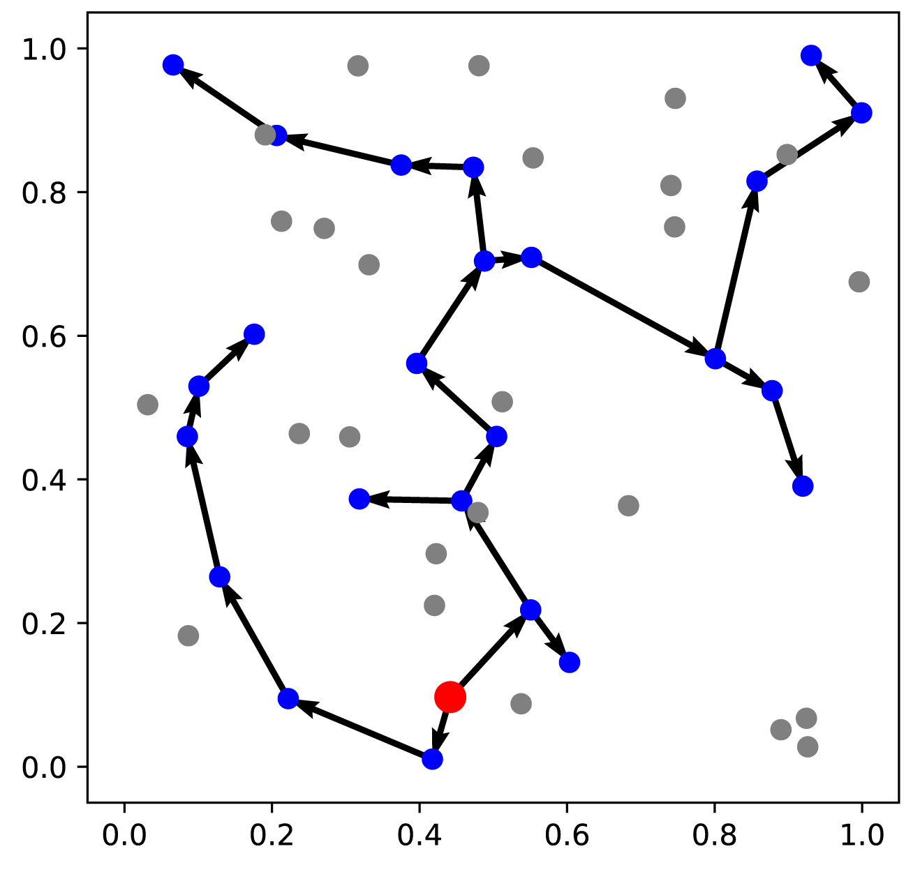
(c) STP ($|V^{\prime}|=25$) of Obj. $3.54$

Figure 7: Example solutions of an instance of size 50 for DCMST ($d=2$), MRCST, STP ($|V^{\prime}|=25$). The terminals are represented by blue nodes, and the edges in solutions by black arrows. The vertex at the beginning of the solution are highlighted in red.

5 Conclusion

In this paper, we introduced a unified framework called NeuroPrim for solving various spanning tree problems on Euclidean space, by defining the MDP for general combinatorial optimization problems on graphs. Our framework achieves near-optimal results in a short time for the DCMST, MRCST and STP problems, without requiring extensive problem-related knowledge. Moreover, it generalizes well to larger instances. Notably, our approach can be extended to solve a wider range of combinatorial optimization problems beyond spanning tree problems.

Looking ahead, there is a need to explore more general methods for solving combinatorial optimization problems. While there are existing open source solution frameworks such as [37, 82], they often rely on designing specific algorithm components for individual problems. Additionally, scaling up to larger problems poses a challenge, as the attention matrix may become too large to store in memory. A possible solution to this is to use local attention within a neighborhood, rather than global attention, which may unlock further potential for the efficiency of our algorithm.

References

- [1] Agarwal Y K, Venkateshan P. New valid inequalities for the optimal communication spanning tree problem. INFORMS Journal on Computing, 2019, 31: 268–284
- [2] Ahmed R, Turja M A, Sahneh F D, et al. Computing Steiner trees using graph neural networks. arXiv:2108.08368, 2021
- [3] Andrade R, Lucena A, Maculan N. Using Lagrangian dual information to generate degree constrained spanning trees. Discrete Applied Mathematics, 2006, 154: 703–717
- [4] Arora S. Polynomial time approximation schemes for Euclidean traveling salesman and other geometric problems. Journal of the ACM, 1998, 45: 753–782
- [5] Bastos M P, Ribeiro C C. Reactive tabu search with path-relinking for the Steiner problem in graphs. Boston, MA: Springer US, 2002, 15: 39–58
- [6] Bello I, Pham H, Le Q V, et al. Neural combinatorial optimization with reinforcement learning. arXiv preprint arXiv:1611.09940, 2017
- [7] Bicalho L H, da Cunha A S, Lucena A. Branch-and-cut-and-price algorithms for the degree constrained minimum spanning tree problem. Computational Optimization and Applications, 2016, 63: 755–792
- [8] Boldon B, Kumar N. Minimum-weight degree-constrained spanning tree problem: heuristics and implementation on an SIMD parallel machine. Parallel Computing, 1996, 14
- [9] Bonnet É, Sikora F, The PACE 2018 parameterized algorithms and computational experiments challenge: The third iteration. In: IPEC, 2018
- [10] Borůvka O, O jisíém problému minimálním, 1926., 24
- [11] Bouchachia A, Prossegger M. A hybrid ensemble approach for the Steiner tree problem in large graphs: A geographical application. Applied Soft Computing, 2011, 11: 5745–5754
- [12] Bresson X, Laurent T. The Transformer network for the traveling salesman problem. arXiv preprint arXiv:2103.03012, 2021
- [13] Bui T N, Deng X H, Zrncic C M. An improved ant-based algorithm for the degree-constrained minimum spanning tree problem. IEEE Transactions on Evolutionary Computation, 2012, 16: 266–278
- [14] Bui T N, Zrncic C M. An ant-based algorithm for finding degree-constrained minimum spanning tree. In: Proceedings of the 8th Annual Conference on Genetic and Evolutionary Computation - GECCO ’06, Seattle, Washington, USA: ACM Press, 2006, 11
- [15] Byrka J, Grandoni F, Rothvoß T, et al. An improved LP-based approximation for steiner tree. In: Proceedings of the 42nd ACM Symposium on Theory of Computing - STOC ’10, Cambridge, Massachusetts, USA: ACM Press, 2010, 583
- [16] Caccetta L, Hill S P. A branch and cut method for the degree-constrained minimum spanning tree problem. Networks, 2001, 37: 74–83
- [17] Campos R, Ricardo M. A fast algorithm for computing minimum routing cost spanning trees. Computer Networks, 2008, 52: 3229–3247
- [18] Chlebík M, Chlebíková J. The Steiner tree problem on graphs: Inapproximability results. Theoretical Computer Science, 2008, 406: 207–214
- [19] Choque J N C. Optimal communication spanning tree. Mestrado em Ciência da Computação, Universidade de São Paulo, São Paulo, 2021
- [20] da Cunha A S, Lucena A. Lower and upper bounds for the degree-constrained minimum spanning tree problem. Networks, 2007, 50: 55–66
- [21] Dai H J, Khalil E B, Zhang Y Y, et al. Learning combinatorial optimization algorithms over graphs. arXiv:1704.01665, 2018
- [22] de Aragão M P, Uchoa E, Werneck R F. Dual heuristics on the exact solution of large Steiner problems. Electronic Notes in Discrete Mathematics, 2001, 7: 150–153
- [23] Delbem A C B, de Carvalho A, Policastro C A, et al. Node-depth encoding for evolutionary algorithms applied to network design. In: Kanade T, Kittler J, Kleinberg J M, Mattern F, Mitchell J C, Naor M, Nierstrasz O, Rangan C P, Steffen B, Sudan M, Terzopoulos D, Tygar D, Vardi M Y, Weikum G, Deb K, eds. Genetic and Evolutionary Computation – GECCO 2004, Berlin, Heidelberg: Springer Berlin Heidelberg, 2004, 3102: 678–687
- [24] Ding M, Han C Y, Guo T D. High generalization performance structured self-attention model for knapsack problem. Discrete Mathematics, Algorithms and Applications, 2021, 13: 2150076
- [25] Doan M N. An effective ant-based algorithm for the degree-constrained minimum spanning tree problem. In: 2007 IEEE Congress on Evolutionary Computation, Singapore: IEEE, 2007, 485–491
- [26] Drori I, Kharkar A, Sickinger W R, et al. Learning to solve combinatorial optimization problems on real-world graphs in linear time. arXiv:2006.03750, 2020
- [27] Du H Z, Yan Z, Xiang Q, et al. Vulcan: Solving the Steiner tree problem with graph neural networks and deep reinforcement learning, arXiv:2111.10810, 2021
- [28] Duin C, Voß S, Efficient path and vertex exchange in steiner tree algorithms. Networks, 1997, 29: 89–105
- [29] Esbensen H. Computing near-optimal solutions to the steiner problem in a graph using a genetic algorithm. Networks, 1995, 26: 173–185
- [30] Fages J G, Lorca X, Rousseau L M. The salesman and the tree: the importance of search in CP. Constraints, 2016, 21: 145–162
- [31] Fischetti M, Lancia G, Serafini P. Exact algorithms for minimum routing cost trees. Networks, 2002, 39: 161–173
- [32] Furer M, Raghavachari B, Approximating the minimum-degree Steiner tree to within one of optimal. Journal of Algorithms, 1994, 17: 409–423
- [33] Garey M R, Johnson D S. Computers and Intractability: A Guide to the Theory of NP-completeness, 27th ed., ser. A Series of Books in the Mathematical Sciences. New York: Freeman, 1979.
- [34] Goemans M. Minimum bounded degree spanning trees. In 2006 47th Annual IEEE Symposium on Foundations of Computer Science (FOCS’06), Berkeley, CA, USA: IEEE, 2006, 273–282
- [35] Guo T D, Han C Y, Tang S Q. Machine learning methods for combinatorial optimization. Beijing: Science Press, 2019
- [36] Guo T D, Han C Y, Tang S Q, et al. Solving combinatorial problems with machine learning methods. In: Du D Z, Pardalos P M, Zhang Z, eds. Nonlinear Combinatorial Optimization, Cham: Springer International Publishing, 2019, 147: 207–229
- [37] Hubbs C D, Perez H D, Sarwar O, et al. OR-Gym: A reinforcement learning library for operations research problems. arXiv preprint arXiv:2008.06319, 2020
- [38] Huy N V, Nghia N D. Solving graphical Steiner tree problem using parallel genetic algorithm. In: 2008 IEEE International Conference on Research, Innovation and Vision for the Future in Computing and Communication Technologies. Ho Chi Minh City, Vietnam: IEEE, 2008, 29–35
- [39] Johnson D S, Lenstra J K, Kan A H G R. The complexity of the network design problem. Networks, 1978, 8: 279–285
- [40] Julstrom B A. The blob code is competitive with edge-sets in genetic algorithms for the minimum routing cost spanning tree problem. In: Proceedings of the 2005 Conference on Genetic and Evolutionary Computation - GECCO ’05, Washington DC, USA: ACM Press, 2005: 585-590
- [41] Kapsalis A, Rayward-Smith V J, Smith G D. Solving the graphical Steiner tree problem using genetic algorithms. The Journal of the Operational Research Society, 1993 44: 397–406
- [42] Karp R M. Reducibility among combinatorial problems. In: Complexity of computer computations, 1972, 85–103
- [43] Khakhulin T, Schutski R, Oseledets I. Learning elimination ordering for tree decomposition problem. In: Learning Meets Combinatorial Algorithms at NeurIPS2020. 2020
- [44] Kingma D P, Ba J. Adam: A method for stochastic optimization. arXiv preprint arXiv:1412.6980, 2017
- [45] Koch T, Martin A. Solving Steiner tree problems in graphs to optimality. Networks, 1998, 32: 207–232
- [46] Kool W, Van Hoof H, and Welling M. Attention, learn to solve routing problems!. arXiv:1803.08475, 2019
- [47] Kruskal J B, On the shortest spanning subtree of a graph and the traveling salesman problem. 1956
- [48] Kwon Y D, Choo J, Kim B, et al. POMO: Policy optimization with multiple optima for reinforcement learning. Advances in Neural Information Processing Systems, 2020, 33: 21188–21198
- [49] Leitner M, Ljubić I, Luipersbeck M, et al. A dual ascent-based branch-and-bound framework for the prize-collecting Steiner tree and related problems. INFORMS Journal on Computing,2018, 30: 402–420
- [50] Lucena A, Beasley J E. A branch and cut algorithm for the Steiner problem in graphs. Networks, 1998, 31: 39–59
- [51] Masone A, Nenni M E, Sforza A, et al. The minimum routing cost tree problem: State of the art and a core-node based heuristic algorithm. Soft Computing, 2019, 23: 2947–2957
- [52] Narula S C, Ho C A, Degree-constrained minimum spanning tree. Computers & Operations Research, 1980, 7: 239–249
- [53] Nazari M, Oroojlooy A, Snyder L V, et al. Reinforcement learning for solving the vehicle routing problem. Advances in Neural Information Processing Systems, 2018, 31
- [54] Polzin T, Daneshmand S V. Improved algorithms for the Steiner problem in networks. Discrete Applied Mathematics, 2001, 112: 263–300
- [55] Presti G L, Re G L, Storniolo P, et al. A grid enabled parallel hybrid genetic algorithm for SPN. In: Kanade T, Kittler J, Kleinberg J M, Mattern F, Mitchell J C, Naor M, Nierstrasz O, Rangan C P, Steffen B, Sudan M, Terzopoulos D, Tygar D, Vardi M Y, Weikum G, Bubak M, van Albada G D, Sloot P M A, Dongarra J, eds. Computational Science - ICCS 2004, Berlin, Heidelberg: Springer Berlin Heidelberg, 2004, 3036: 156–163
- [56] Prim R C. Shortest connection networks and some generalizations. Bell System Technical Journal, 1957, 36: 1389–1401
- [57] Qu R, Xu Y, Castro J P, et al. Particle swarm optimization for the Steiner tree in graph and delay-constrained multicast routing problems. Journal of Heuristics, 2013, 19: 317–342
- [58] Raidl G R, Julstrom B A. Edge sets: an effective evolutionary coding of spanning trees. IEEE Transactions on Evolutionary Computation, 2003, 7: 225–239
- [59] Ribeiro C C, De Souza M C, Tabu search for the Steiner problem in graphs. Networks, 2000, 36: 138–146
- [60] Ribeiro C C, Uchoa E, Werneck R F. A hybrid GRASP with perturbations for the Steiner problem in graphs. INFORMS Journal on Computing, 2002, 14: 228–246
- [61] Sattari S, A metaheuristic algorithm for the minimum routing cost spanning tree problem. 2015, 14
- [62] Sattari S, Didehvar F. Variable neighborhood search approach for the minimum routing cost spanning tree problem. Int J Oper Res, 2013, 10: 153–160
- [63] Scott A J. The optimal network problem: some computational procedures. Transportation Research, 1969, 3: 201–210
- [64] Singh A. A new heuristic for the minimum routing cost spanning tree problem. In: 2008 International Conference on Information Technology, Bhunaneswar, Orissa, India: IEEE, 2008, 9–13
- [65] Singh A, Sundar S. An artificial bee colony algorithm for the minimum routing cost spanning tree problem. Soft Computing, 2011, 15: 2489–2499
- [66] Singh M, Lau L C. Approximating minimum bounded degree spanning trees to within one of optimal. Journal of the ACM, 2015, 62: 1–19
- [67] Singh K, Sundar S. A hybrid genetic algorithm for the degree-constrained minimum spanning tree problem. Soft Computing, 2020, 24: 2169–2186
- [68] Sutton R S, McAllester D, Singh S, et al. Policy gradient methods for reinforcement learning with function approximation. Advances in Neural Information Processing Systems, 1999, 12
- [69] Takahashi H, Matsuyama A. An approximate solution for the Steiner problem in graphs, 1980, 5
- [70] Tan Q P. A genetic approach for solving minimum routing cost spanning tree problem. International Journal of Machine Learning and Computing, 2012, 410–414
- [71] Tan Q P. A heuristic approach for solving minimum routing cost spanning tree problem. International Journal of Machine Learning and Computing, 2012, 406–409
- [72] Tilk C, Irnich S, Combined column-and-row-generation for the optimal communication spanning tree problem. Computers & Operations Research, 2018, 93: 113–122
- [73] Uchoa E, Werneck R F. Fast local search for the steiner problem in graphs. ACM Journal of Experimental Algorithmics, 2012, 17: 2–1
- [74] Vaswani A, Shazeer N, Parmar N, et al. Attention is all you need. Advances in Neural Information Processing Systems, 2017, 30
- [75] Vinyals O, Fortunato M, Jaitly N. Pointer networks. Advances in Neural Information Processing Systems, 2015, 28
- [76] Wang C G, Han C Y, Guo T D, et al. Solving uncapacitated p-median problem with reinforcement learning assisted by graph attention networks. Applied Intelligence, 2022
- [77] Wang C G, Yang Y D, Slumbers O, et al. A game-theoretic approach for improving generalization ability of TSP solvers. arXiv:2110.15105, 2022
- [78] Wang Q, Hao Y S, Cao J. Learning to traverse over graphs with a Monte Carlo tree search-based self-play framework. Engineering Applications of Artificial Intelligence, 2021, 105: 104422
- [79] Wong R T. Worst-case analysis of network design problem heuristics. SIAM Journal on Algebraic Discrete Methods, 1980, 1: 51–63
- [80] Wu B Y, Lancia G, Bafna V, et al. A polynomial-time approximation scheme for minimum routing cost spanning trees. SIAM Journal on Computing, 2000, 29: 761–778
- [81] Zetina C A, Contreras I, Fernández E, et al. Solving the optimum communication spanning tree problem. European Journal of Operational Research, 2019, 273: 108–117
- [82] Zheng W J, Wang D L, Song F G. OpenGraphGym: A parallel reinforcement learning framework for graph optimization problems. In: Krzhizhanovskaya V V, Závodszky G, Lees M H, Dongarra J J, Sloot P M A, Brissos S, Teixeira J, eds. Computational Science – ICCS 2020, Cham: Springer International Publishing, 2020, 12141: 439–452