Bio-inspired periodic panels optimised for acoustic insulation

Abstract

The design of structures that can yield efficient sound insulation performance is a recurring topic in the acoustic engineering field. Special attention is given to panels, which can be designed using several approaches to achieve considerable sound attenuation. In a previous work, we have presented the concept of thickness-varying periodic plates with optimised profiles to inhibit flexural wave energy propagation. In this work, motivated by biological structures that present multiple locally-resonant elements able to cause acoustic cloaking, we extend our shape optimisation approach to design panels that achieve improved acoustic insulation performance using either thickness-varying profiles or locally-resonant attachments. The optimisation is performed using numerical models that combine the Kirchhoff plate theory and the plane wave expansion method. Our results indicate that panels based on locally resonant mechanisms have the advantage of being robust against variation in the incidence angle of acoustic excitation and, therefore, are preferred for single-leaf applications.

1 Introduction

Sound insulation has been one of the most studied subjects in various fields of Engineering [1, 2, 3]. Common solutions to achieve this objective include (i) the use of absorptive materials chosen to accept acoustic energy and dissipate it in the form of heat [4, 5], and (ii) the use of systems with a large impedance mismatch in the acoustic transmission path, thus reflecting the sound energy, instead of transmitting it [6, 7].

Recent findings in the field of Biology have shown that the wings of moths and butterflies are endowed with specialized double-layered scales with nanostructures that are able to effectively perform ultrasound absorption and create an acoustic camouflage against predators [8, 9]. In this case, multiple scales which individually contribute as sub-wavelength resonating elements are connected via a thin membrane to absorb impinging waves over a wide frequency range [10]. Such intriguing capabilities may certainly entice the design of novel acoustic metamaterials (MMs) for various engineering applications [11]. Especially, a remarkable resemblance with panels with embedded resonators and their application in noise insulation is promptly noticed.

Panels are a common solution for sound insulation in many engineering vibroacoustic applications [12]. In this case, the control of noise in the low-frequency regions depends on the stiffness and/or mass of the panel [13], which may lead to increasingly large panel thickness to improve acoustic performance. To avoid this issue, a number of panel designs such as sandwich [14], honeycomb [15], and fibre-reinforced composite panels [16] are capable of combining high stiffness with low mass. These solutions may further benefit from the use of (i) phononic crystals (PCs) and (ii) periodic MMs, since these may possess phononic band gaps, i.e., frequency ranges where no free wave propagation is allowed in the solid medium [17]. Such frequency bands arise typically due to the mechanisms of (i) Bragg scattering [18], in which case the frequency range is associated with the periodicity of the medium, and (ii) local resonance [19], where Fano-like interference is capable of opening band gaps in the sub-wavelength scale [20].

Claeys et al. have discussed the acoustic radiation efficiency of local resonance-based MMs [21] and proposed its use in the design of a lightweight acoustic insulator [22]. The use of distributed resonators has also been investigated as an option to create MMs for both thin [23] and thick [24] plate structures using the plane wave expansion (PWE) method to achieve an improved sound transmission loss (STL). Furthermore, Van Belle et al. have demonstrated [25] that both PCs and MMs are able to improve the STL of infinite plates. For MMs, this reduction occurs inside the band gap regions, due to sub-wavelength vibration suppression, while, for PCs, these occur outside the band gap regions due to specific vibration patterns. However, investigations on the use of corrugated profiles [26, 27] to design both PCs and MMs for vibroacoustic applications remain largely unexplored.

In a previous work, we have proposed the optimisation of Fourier coefficients describing the shape of periodic plates for maximising Bragg-type band gaps for structural applications [28]. In this work, motivated by the characteristics obtained by the combination of resonating elements connected via a thin membrane present in moth wings, we propose the extension of our previously presented optimisation approach to design (i) thickness-varying panels or (ii) panels embedded with multiple resonating elements for sound insulation applications. The optimisation is performed for the normal incidence of impinging waves and is also assessed for the cases of oblique and diffuse incidence. Both single- and double-leaf panels are investigated.

In Section 2, we revise the concepts relative to thickness-varying plates and periodically distributed resonators and their corresponding Fourier series representation. Section 3 presents some key concepts and definitions, which are needed for the analysis of the vibroacoustic behaviour. Section 4 briefly reviews the formulation for the vibroacoustic behaviour of a single-leaf infinite panel and its extension to the double-leaf case using the PWE method, describing also the metrics related with the calculation of the STL and radiated acoustic pressure, as well as analytical solutions. Section 5 presents the optimisation problem, stating its cost function, optimised variables, and constraints, and Section 6 presents the obtained numerical results. Concluding remarks are drawn in Section 7.

2 Periodic media and Fourier series representation

2.1 Plate displacement field

Even though the sound transmission characteristics of simple panels are commonly obtained considering analytical solutions [29], numerical formulations are generally required for complex structures [30, 31]. The PWE method can be applied to determine the wave propagation characteristics of one-, two- [32], and three-dimensional periodic MMs [33], and its improved computational efficiency, when compared with finite element-based methods [34], further motivates its use for optimisation problems [35, 36, 37]. The PWE method requires the analytical description of the displacement field of the medium and its material/geometric properties using their corresponding Fourier series, which are described in this section.

Consider a plate lying in the $xy$-plane with coordinates described by the two-dimensional position vector $\mathbf{r}=x\hat{\mathbf{i}}+y\hat{\mathbf{j}}$. The plate transverse displacement $u_{z}(\mathbf{r},t)$ can be described using [28]

$$u_{z}(\mathbf{r},t)=e^{-\text{i}\omega t}\sum_{\mathbf{G}}\hat{u}_{z}(\mathbf{G})e^{\text{i}(\mathbf{k}+\mathbf{G})\cdot\mathbf{r}}\,,$$ (1)

where $\hat{u}_{z}(\mathbf{G})$ represents spatial Fourier coefficients, the wave propagation in the plate is described by the direction and wavelength given by the wave vector $\mathbf{k}=k_{x}\hat{\mathbf{i}}+k_{y}\hat{\mathbf{j}}$, and $\mathbf{G}$ is the reciprocal lattice vector, which is given, for a square plate of side length $L$, by

$$\mathbf{G}=n_{x}\frac{2\pi}{L}\hat{\mathbf{i}}+n_{y}\frac{2\pi}{L}\hat{\mathbf{j}}=\mathbf{G}_{n_{x},\,n_{y}}\,,$$ (2)

for integers $\{n_{x},\,n_{y}\}\in\mathbb{Z}$. If indexes $n_{x}$ and $n_{y}$ are in the range $[-N_{\max},N_{\max}]$, one obtains a number of plane waves equal to $n_{G}=(1+2N_{\max})^{2}$.

In the case of a thin plate where the effects of rotational inertia and shear strain are negligible, the Kirchhoff plate theory can be used to obtain the corresponding elastodynamic equations, which can be written in the rectangular coordinate system as [38, 39]

$$\small\frac{\partial^{2}}{\partial x^{2}}\bigg{[}D\bigg{(}\frac{\partial^{2}u_{z}}{\partial x^{2}}+\nu\frac{\partial^{2}u_{z}}{\partial y^{2}}\bigg{)}\bigg{]}+2\frac{\partial^{2}}{\partial x\partial y}\bigg{[}D(1-\nu)\frac{\partial^{2}u_{z}}{\partial x\partial y}\bigg{]}+\frac{\partial^{2}}{\partial y^{2}}\bigg{[}D\bigg{(}\nu\frac{\partial^{2}u_{z}}{\partial x^{2}}+\frac{\partial^{2}u_{z}}{\partial y^{2}}\bigg{)}\bigg{]}+\rho h\frac{\partial^{2}u_{z}}{\partial t^{2}}=q(\mathbf{r},t)\,,$$ (3)

where $\rho$ is the material density, $\nu$ is the Poisson’s ratio, $h$ is the plate thickness, $D=Eh^{3}/12(1-\nu^{2})$ is the plate flexural stiffness, where $E$ is the Young’s modulus, and $q(\mathbf{r},t)$ is the distributed loading on the plate surface, which can include the presence of both fluid loading and the interaction with mass-spring resonators.

The flexural wave speed in plates is given by

$$c=\sqrt[4]{\frac{D}{\rho h}}\sqrt{\omega}\,,$$ (4)

which leads to the relation between the wavelength $\lambda$ and frequency $f$, after substituting $c=\lambda f$ and $\omega=2\pi f$, written as $\lambda=\sqrt[4]{\frac{D}{\rho h}}\,\sqrt{\frac{2\pi}{f}}$, where the relation $h\ll\lambda$ must hold true for all the analysed frequencies for the Kirchhoff plate theory to be valid.

2.2 Plate thickness

The periodic thickness of the thin plate (figure 1) can be described by the spatial-dependent function $h(\mathbf{r})$ given by

$$h(\mathbf{r})=\sum_{\mathbf{G}}\hat{h}(\mathbf{G})\,e^{\text{i}\mathbf{G}\cdot\mathbf{r}}\,,$$ (5)

where the Fourier coefficients of $h(\mathbf{r})$ can be written, for integers $n_{x}$ and $n_{y}$ (Eq. (2)) as

$$\hat{h}(\mathbf{G}_{n_{x},\,n_{y}})=\hat{h}_{n_{x},\,n_{y}}\,,$$ (6)

leading to the expression of the thickness profile of a plate in terms of the coefficients of the corresponding reciprocal lattices as

$$h(\mathbf{r})=\sum_{n_{y}}\sum_{n_{x}}\hat{h}_{n_{x},\,n_{y}}e^{\text{i}\mathbf{G}_{n_{x},\,n_{y}}\cdot\mathbf{r}}\,.$$ (7)

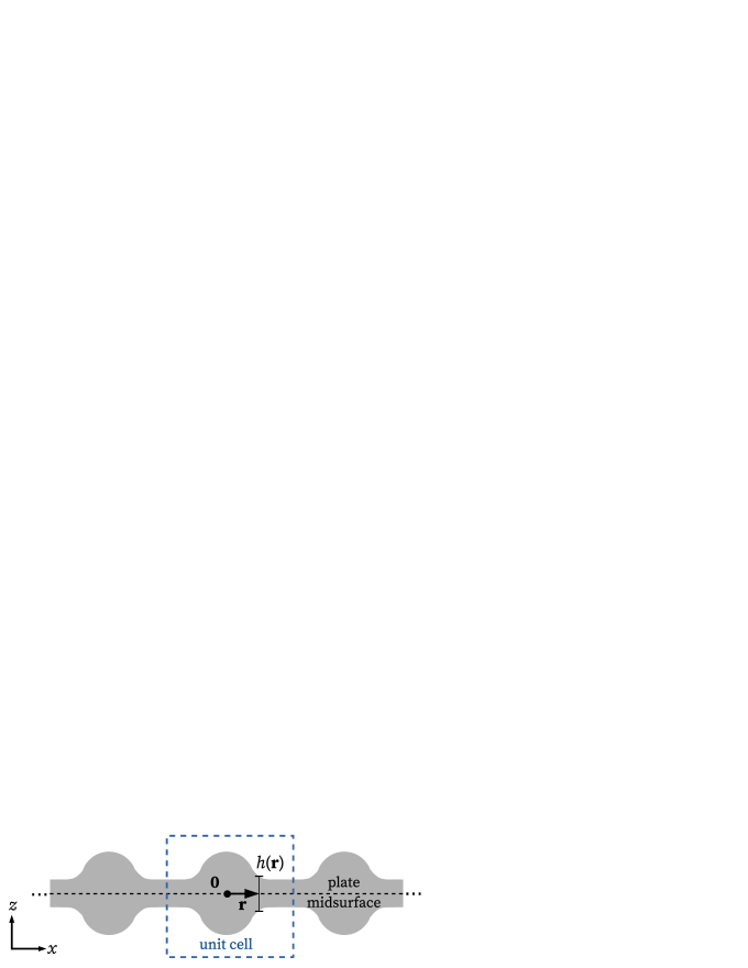
Figure 1: Thickness $h(\mathbf{r})$ for a periodic thin plate lying on the $xy$ plane.

The space-dependent flexural rigidity of the plate is given by $D(\mathbf{r})=\frac{Eh^{3}(\mathbf{r})}{12(1-\nu^{2})}$, which has the same period as $h(\mathbf{r})$, and can also be expressed in terms of its Fourier series using

$$D(\mathbf{r})=\sum_{\mathbf{G}}\hat{D}(\mathbf{G})\,e^{\text{i}\mathbf{G}\cdot\mathbf{r}}\,,$$ (8)

with Fourier coefficients $\hat{D}(\mathbf{G})$ that can be obtained from the coefficients $\hat{h}(\mathbf{G})$ using the procedure described in [28].

The set of coefficients $\hat{h}_{n_{x},\,n_{y}}$ can be determined such that a thickness profile which presents the best possible sound insulation performance is obtained, while respecting imposed geometric constraints. The optimisation problem with its associated metrics and constraints are defined in Section 5.

2.3 Mass-spring resonators

The inclusion of periodic resonator-type structures is an interesting option to control vibrations in the sub-wavelength scale [40, 41, 42, 43]. Here we consider a set of $n_{r}$ independent ideal mass-spring resonators, where each resonator is defined by a point mass $m_{p}$ and a spring stiffness $k_{p}$ (figure 2a), fixed to the plate at coordinates $\mathbf{r}_{p}=x_{p}\hat{\mathbf{i}}+y_{p}\hat{\mathbf{j}}$ (figure 2b). Since the plate is periodic, the $p$-th resonator has coordinates which are restricted to the unit cell domain, i.e., $-L/2<\{x_{p},\,y_{p}\}<L/2$, with a corresponding out-of-plane displacement, $u_{p}(\mathbf{r}_{p},t)$, exerting a force with intensity $F_{p}(\mathbf{r}_{p},t)$ on the plate (figure 2c), which holds for $p=\{1,\,2,\,\dots,n_{r}\}$.

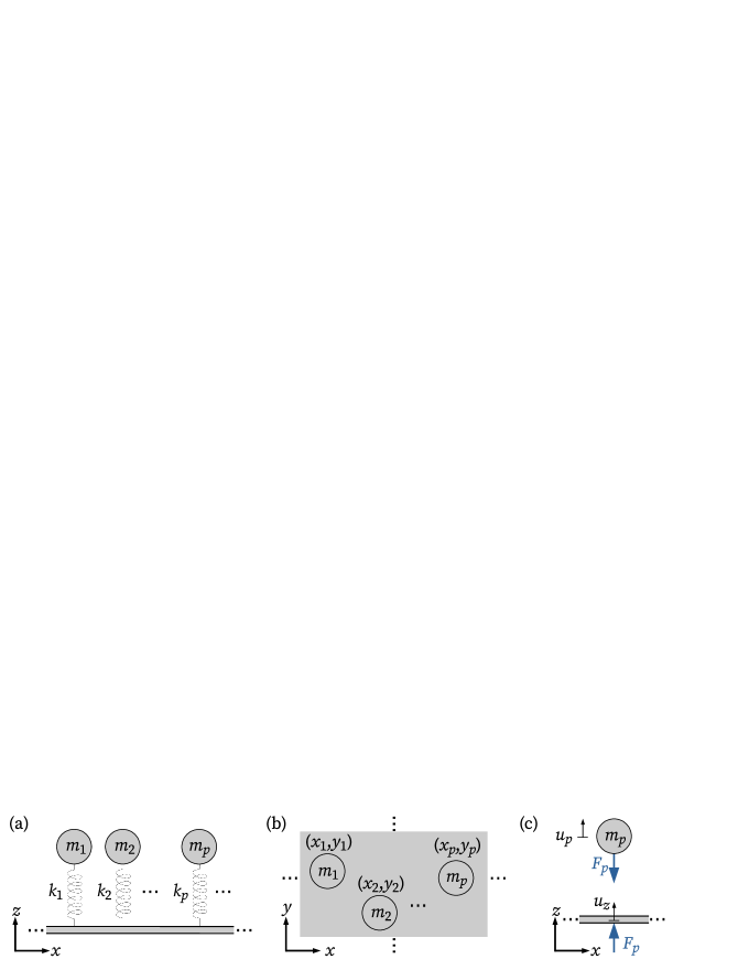
Figure 2: Distribution of mass-spring resonators on a thin plate. (a) The $p$-th resonator is composed of a mass $m_{p}$ and a spring $k_{p}$ (b) with coordinates $(x_{p},\,y_{p})$. (c) The displaced mass exerts an out-of-plane force with intensity $F_{p}$ at the plate.

The periodic force $q_{r}(\mathbf{r},t)$ applied by the set of resonators on the plate can be described by

$$q_{r}(\mathbf{r},t)=e^{-\text{i}\omega t}\sum_{p}\sum_{\mathbf{R}}F_{p}(\mathbf{r}_{p}+\mathbf{R},\,t)\,\delta(\mathbf{r}-(\mathbf{r}_{p}+\mathbf{R}))\,,$$ (9)

where $\mathbf{R}=m_{x}L\,\hat{\mathbf{i}}+m_{y}L\,\hat{\mathbf{j}}$, $\{m_{x},\,m_{y}\}\in\mathbb{Z}$, is the square lattice direct vector, representing the plate periodicity, and $\delta(\mathbf{r}-(\mathbf{r}_{p}+\mathbf{R}))=\delta(x-(x_{p}+m_{x}L))\,\delta(y-(y_{p}+m_{y}L))$ is the two-dimensional Dirac delta function [42], which implies $\delta(\mathbf{r}\neq\mathbf{r}_{p}+\mathbf{R})=0$.

The periodic spring force can be related with the dynamic equation of the $p$-th resonator mass by

$$F_{p}(\mathbf{r}_{p}+\mathbf{R},\,t)=k_{p}(u_{p}(\mathbf{r}_{p}+\mathbf{R},\,t)-u_{z}(\mathbf{r}_{p}+\mathbf{R},\,t))=-m_{p}\ddot{u}_{p}(\mathbf{r}_{p}+\mathbf{R},\,t)\,,$$ (10)

where both the resonator and plate displacements, respectively, $u_{p}(\mathbf{r},t)$ and $u_{z}(\mathbf{r},t)$, are evaluated at the points $\mathbf{r}_{p}+\mathbf{R}$ and can be used, by considering harmonic displacements denoted in the form $f(\mathbf{r},\,t)=e^{-\text{i}\omega t}f(\mathbf{r})$, to write

$$F_{p}(\mathbf{r},t)=\frac{k_{p}m_{p}\omega^{2}}{k_{p}-m_{p}\omega^{2}}u_{z}(\mathbf{r},t)\,.$$ (11)

Equation (1) implies $u_{z}(\mathbf{r}_{p}+\mathbf{R})=e^{\text{i}\mathbf{k}\cdot\mathbf{R}}u_{z}(\mathbf{r}_{p})$, which can be used with the relation given by [34, 41]

$$\sum_{\mathbf{R}}e^{\text{i}\mathbf{k}\cdot\mathbf{R}}\delta(\mathbf{r}-(\mathbf{r}_{p}+\mathbf{R}))=\frac{1}{S}\sum_{\mathbf{G}}e^{\text{i}(\mathbf{k}+\mathbf{G})\cdot\mathbf{r}}e^{-\text{i}(\mathbf{k}+\mathbf{G})\cdot\mathbf{r}_{p}}\,,$$ (12)

where $S=L^{2}$, and combined with Eq. (9) and (11) using distinct summation indexes, to write

$$q_{r}(\mathbf{r},t)=e^{-\text{i}\omega t}\sum_{p}\frac{k_{p}m_{p}\omega^{2}}{k_{p}-m_{p}\omega^{2}}\frac{1}{S}\sum_{\mathbf{G}}e^{\text{i}(\mathbf{k}+\mathbf{G})\cdot\mathbf{r}}e^{-\text{i}(\mathbf{k}+\mathbf{G})\cdot\mathbf{r}_{p}}\,\sum_{\mathbf{H}}\hat{u}_{z}(\mathbf{H})e^{\text{i}(\mathbf{k}+\mathbf{H})\cdot\mathbf{r}_{p}}\,.$$ (13)

This equation can be included as corresponding loading terms to account for locally resonant mechanisms present in the plate.

3 Fluid-structure interaction

In this section, we introduce the basic definitions associated with the analysis of the vibroacoustic problem, including the representation of acoustic waves and the fluid-structure coupling formulation. Since we are concerned with acoustic insulation applications, the fluid is generally considered as air, although the presented denomination has been chosen for the sake of generality [31].

Consider an incident plane wave ($P_{i}$) propagating through a fluid, which impinges on an infinite thin plate. The plate immersed in fluid will be referred to as panel. The resulting motion of the plate excites the surrounding fluid, which causes the formation of both reflected ($P_{r}$) and transmitted ($P_{t}$) plane waves, respectively, at the same and the opposing sides of the incident face (figure 3a). The wavenumber components of the incident wave can be described using the angles $\varphi$, with respect to the $z$-axis, and its projection in the $xy$-plane with an angle $\theta$, with respect to the $x$-axis (figure 3b).

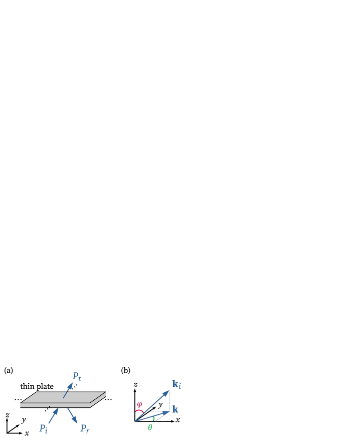
Figure 3: Acoustic plane waves: (a) incident ($P_{i}$), reflected ($P_{r}$), and transmitted ($P_{t}$) waves; (b) wave vector of the incident wave $\mathbf{k}_{i}$, its component $\mathbf{k}$ in the $xy$-plane, and angles $\varphi$ and $\theta$ for spherical coordinates projection.

The incident plane wave can thus be expressed as [31]

$$P_{i}(\mathbf{r},z,t)=e^{-\text{i}\omega t}\overline{P}_{i}e^{\text{i}\mathbf{k}\cdot\mathbf{r}}e^{\text{i}k_{z}z}\,,$$ (14)

where $\overline{P}_{i}$ represents the incident plane wave complex amplitude, the in-plane components of the incident wave vector $\mathbf{k}_{i}$ are represented by $\mathbf{k}$ and the out-of-plane components by $k_{z}$, with wavenumber components described in the Cartesian coordinate system using

$$k_{x}=k_{0}\sin\varphi\cos\theta\,,k_{y}=k_{0}\sin\varphi\sin\theta\,,k_{z}=k_{0}\cos\varphi\,,$$ (15)

where $k_{0}=|\mathbf{k}_{i}|=\omega/c_{0}$ is the wavenumber of the incident wave, with $\omega$ the angular frequency of the incident wave, and $c_{0}$ the speed of sound in air. The wavelength induced in the plate by the incident plane wave is given by $\sqrt{k_{x}^{2}+k_{y}^{2}}=|\mathbf{k}|=k_{0}\sin\varphi$ and is named trace wavenumber [13], which becomes zero for the case of normal incidence.

The reflected and transmitted waves can be described, respectively, similarly to Eq. (1), as [24]

$$P_{r}(\mathbf{r},z,t) =e^{-\text{i}\omega t}\sum_{\mathbf{G}}\hat{P}_{r}(\mathbf{G})e^{\text{i}(\mathbf{k}+\mathbf{G})\cdot\mathbf{r}}e^{-\text{i}k_{za}(\mathbf{G})z}\,,$$ (16a)

$$P_{t}(\mathbf{r},z,t) =e^{-\text{i}\omega t}\sum_{\mathbf{G}}\hat{P}_{t}(\mathbf{G})e^{\text{i}(\mathbf{k}+\mathbf{G})\cdot\mathbf{r}}e^{\text{i}k_{za}(\mathbf{G})z}\,,$$ (16b)

where $k_{za}(\mathbf{G})$ is the $z$-direction component of the wave vectors associated with the reflected and transmitted waves, which depend on the wavenumber of the incident wave and the trace wavenumber and can be calculated according to

$$k_{za}(\mathbf{G}) =\sqrt{k_{0}^{2}-|\mathbf{k}+\mathbf{G}|^{2}}\,,\text{ if }k_{0}^{2}\geq|\mathbf{k}+\mathbf{G}|^{2}\,,$$ (17a)

$$k_{za}(\mathbf{G}) =\text{i}\sqrt{|\mathbf{k}+\mathbf{G}|^{2}-k_{0}^{2}}\,,\text{if }k_{0}^{2}<|\mathbf{k}+\mathbf{G}|^{2}\,.$$ (17b)

Both reflected and transmitted sound pressures have $n_{G}$ Fourier coefficients ($\hat{P}_{r}(\mathbf{G})$ and $\hat{P}_{t}(\mathbf{G})$, respectively), which must be determined with the application of the fluid-structure coupling equations.

The incident plane wave can be rewritten, keeping the same notation as Eq. (16), as

$$P_{i}(\mathbf{r},z,t)=e^{-\text{i}\omega t}\sum_{\mathbf{G}}\hat{P}_{i}(\mathbf{G})e^{\text{i}(\mathbf{k}+\mathbf{G})\cdot\mathbf{r}}e^{\text{i}k_{z}z}\,,$$ (18)

where $\hat{P}_{i}(\mathbf{G}=\mathbf{0})=\overline{P}_{i}$ and $\hat{P}_{i}(\mathbf{G}\neq\mathbf{0})=0$.

Henceforth, we shall suppose that the plate is thin enough so that the effects of waves applying pressure at the lower and upper sides of the panel can be approximated by their application at the plate midsurface ($z=0$). Acoustic waves apply pressures in opposing directions (see figure 3a): the incident and reflected waves create a force in the positive ($+z$) direction, while the transmitted wave creates a force in the negative ($-z$) direction. Such fluid loading $q_{f}=q_{f}(\mathbf{r},t)$ can be written using Eqs. (16) and (18) as

$$q_{f}(\mathbf{r},t)=P_{i}(\mathbf{r},z=0,t)+P_{r}(\mathbf{r},z=0,t)-P_{t}(\mathbf{r},z=0,t)\\ =e^{-\text{i}\omega t}\sum_{\mathbf{G}}\bigg{[}\hat{P}_{i}(\mathbf{G})+\hat{P}_{r}(\mathbf{G})-\hat{P}_{t}(\mathbf{G})\bigg{]}e^{\text{i}(\mathbf{k}+\mathbf{G})\cdot\mathbf{r}}\,.$$ (19)

The continuity of accelerations at the fluid-structure interface can be described as

$$\frac{\partial P}{\partial z}\bigg{|}_{z=z_{0}}=\rho_{0}\omega^{2}u_{z}\big{|}_{z=z_{0}}\,,$$ (20)

where $z_{0}$ is the $z$-coordinate of the fluid-structure interface, and $\rho_{0}$ is the mass density of the fluid. Since here a two-dimensional plate model is used, the transverse displacement is independent of the $z$-coordinate, which implies $u_{z}|_{z=z_{0}}=u_{z}$.

Equation (20) can be evaluated for the incident and reflected waves and expanded using Eqs. (1), (16a), and (18), leading to the relation, for each $\mathbf{G}$, given by

$$\hat{P}_{r}(\mathbf{G})=\frac{k_{z}}{k_{za}(\mathbf{G})}\hat{P}_{i}(\mathbf{G})+\frac{\text{i}\rho_{0}\omega^{2}}{k_{za}(\mathbf{G})}\hat{u}_{z}(\mathbf{G})\,.$$ (21)

An analogous relation can be used for the coupling at the transmitting face, where the continuity of accelerations and Eqs. (16b) and (1) allow to write

$$\hat{P}_{t}(\mathbf{G})=-\frac{\text{i}\rho_{0}\omega^{2}}{k_{za}(\mathbf{G})}\hat{u}_{z}(\mathbf{G})\,.$$ (22)

Equations (21) and (22) can be substituted in Eq. (19) to write

$$q_{f}(\mathbf{r},t)=e^{-\text{i}\omega t}\sum_{\mathbf{G}}\bigg{[}\bigg{(}1+\frac{k_{z}}{k_{za}(\mathbf{G})}\bigg{)}\hat{P}_{i}(\mathbf{G})+2\frac{\text{i}\rho_{0}\omega^{2}}{k_{za}(\mathbf{G})}\hat{u}_{z}(\mathbf{G})\bigg{]}e^{\text{i}(\mathbf{k}+\mathbf{G})\cdot\mathbf{r}}\,,$$ (23)

which represents the equivalent loading imposed on the plate by the incident pressure wave and the fluid-structure interaction.

In the next sections, for the sake of simplicity, the effects of the thickness variation and the inclusion of resonators are presented separately.

4 Sound insulation panels

4.1 Single-leaf formulation

Considering the case of a PC, i.e., a thickness-varying plate without the presence of local resonators, Eqs. (5) and (8) can be used with a summation index of $\mathbf{H}$ for material properties, and Eqs. (23) and (1) with a summation index $\mathbf{G}$ for displacement and acoustic waves in Eq. (3), one obtains

$$e^{-\text{i}\omega t}\sum_{\mathbf{H}}\sum_{\mathbf{G}}\bigg{[}\hat{D}(\mathbf{H})\{[(k_{x}+G_{x})(k_{x}+G_{x}+H_{x})+(k_{y}+G_{y})(k_{y}+G_{y}+H_{y})]^{2}$$ (24)

$$+\nu[(k_{x}+G_{x})(k_{y}+G_{y}+H_{y})-(k_{y}+G_{y})(k_{x}+G_{x}+H_{x})]^{2}\}\hat{u}_{z}(\mathbf{G})-\omega^{2}\rho\hat{h}(\mathbf{H})\hat{u}_{z}(\mathbf{G})$$

$$-\bigg{(}1+\frac{k_{z}}{k_{za}(\mathbf{G})}\bigg{)}\hat{P}_{i}(\mathbf{G})\delta(\mathbf{H})-2\frac{\text{i}\rho_{0}\omega^{2}}{k_{za}(\mathbf{G})}\hat{u}_{z}(\mathbf{G})\delta(\mathbf{H})\bigg{]}e^{\text{i}(\mathbf{k}+\mathbf{G}+\mathbf{H})\cdot\mathbf{r}}=0\,.$$

The orthogonality property of the complex exponential [44, 45] can be used to write, for every $\mathbf{r}$ and $\mathbf{H}$, a set of linear equations, for $i=1,\,\dots,\,n_{G}$, obtained by substituting $\mathbf{H}=\mathbf{G}_{i}-\mathbf{G}_{j}$ and $\mathbf{G}=\mathbf{G}_{j}$, written as

$$\sum_{\mathbf{G}_{j}}\bigg{[}\hat{D}_{ij}\{[(k_{x}+G_{xj})(k_{x}+G_{xi})+(k_{y}+G_{yj})(k_{y}+G_{yi})]^{2}$$ (25)

$$+\nu[(k_{x}+G_{xj})(k_{y}+G_{yi})-(k_{y}+G_{yj})(k_{x}+G_{xi})]^{2}\}-\omega^{2}\rho\hat{h}_{ij}\bigg{]}\hat{u}_{z}(\mathbf{G}_{j})$$

$$-\bigg{(}1+\frac{k_{z}}{k_{za}(\mathbf{G}_{i})}\bigg{)}\hat{P}_{i}(\mathbf{G}_{i})-2\frac{\text{i}\rho_{0}\omega^{2}}{k_{za}(\mathbf{G}_{i})}\hat{u}_{z}(\mathbf{G}_{i})=0\,,$$

where $\hat{D}_{ij}=\hat{D}(\mathbf{G}_{i}-\mathbf{G}_{j})$, $\hat{h}_{ij}=\hat{h}(\mathbf{G}_{i}-\mathbf{G}_{j})$. This previous equation can be simplified as

$$\sum_{\mathbf{G}_{j}}\bigg{[}\hat{D}_{ij}f_{ij}-\omega^{2}\rho\hat{h}_{ij}\bigg{]}\hat{u}_{z}(\mathbf{G}_{j})-2\frac{\text{i}\rho_{0}\omega^{2}}{k_{za}(\mathbf{G}_{i})}\hat{u}_{z}(\mathbf{G}_{i})=\bigg{(}1+\frac{k_{z}}{k_{za}(\mathbf{G}_{i})}\bigg{)}\hat{P}_{i}(\mathbf{G}_{i})\,,$$ (26)

where $f_{ij}=f_{ij}(\mathbf{k},\mathbf{G}_{i},\mathbf{G}_{j})$ is given by

$$\small f_{ij}=[(k_{x}+G_{xj})(k_{x}+G_{xi})+(k_{y}+G_{yj})(k_{y}+G_{yi})]^{2}+\nu[(k_{x}+G_{xj})(k_{y}+G_{yi})-(k_{y}+G_{yj})(k_{x}+G_{xi})]^{2}\,.$$ (27)

Equation (25) represents a set of $n_{G}$ linear equations, which can be rewritten in matrix form last relation allows to determine the Fourier components $\hat{u}_{z}(\mathbf{G})$ using

$$(\widetilde{\mathbf{D}}+\mathbf{D}_{f})\hat{\mathbf{u}}_{z}=\mathbf{f}\,,$$ (28)

where the matrix $\widetilde{\mathbf{D}}$ can be written as

$$\widetilde{\mathbf{D}}=\widetilde{\mathbf{K}}-\omega^{2}\widetilde{\mathbf{M}}\,,$$ (29)

with the components of matrices $\widetilde{\mathbf{K}}$, $\widetilde{\mathbf{M}}$, the diagonal matrix $\mathbf{D}_{f}$, and the vector $\mathbf{f}$ are respectively given by

$$(\widetilde{\mathbf{K}})_{ij}=\hat{D}_{ij}f_{ij}\,,(\widetilde{\mathbf{M}})_{ij}=\rho\hat{h}_{ij}\,,(\mathbf{D}_{f})_{ii}=-2\frac{\text{i}\rho_{0}\omega^{2}}{k_{za}(\mathbf{G}_{i})}\,,(\mathbf{f})_{i}=\bigg{(}1+\frac{k_{z}}{k_{za}(\mathbf{G}_{i})}\bigg{)}\hat{P}_{i}(\mathbf{G}_{i})\,,$$ (30)

and the vector of unknowns is given by

$$\hat{\mathbf{u}}_{z}=\left\{\hat{u}_{z}(\mathbf{G}_{1}),\,\dots,\,\hat{u}_{z}(\mathbf{G}_{n_{G}})\right\}^{T}\,.$$ (31)

In Eq. (28), matrix $\widetilde{\mathbf{D}}$ accounts for the periodic plate dynamic stiffness characteristics, matrix $\mathbf{D}_{f}$ includes the additional impedance associated with the fluid-structure interaction, and vector $\mathbf{f}$ represents the excitation induced by the incident wave pressure. Finally, the vector of Fourier coefficients of the transmitted wave can be represented as

$$\hat{\mathbf{P}}_{t}=\left\{\hat{P}_{t}(\mathbf{G}_{1}),\,\dots,\,\hat{P}_{t}(\mathbf{G}_{n_{G}})\right\}^{T}\,,$$ (32)

which can be directly obtained from the solution of Eq. (28) with the use of Eq. (22). Thus, for each pair of angles indicating the direction of the incident wave ($\varphi$, $\theta$), Eq. (28) can be solved for a given set of angular frequencies, $\omega$, thus yielding the Fourier components relative to the plate displacements, $u_{z}(\mathbf{r},t)$, and, consequently, transmitted waves, $P_{t}(\mathbf{r},z,t)$. This formulation is similar to that presented by Xiao et al. [23], with the proper use of Fourier series coefficients corresponding to the plate thickness variation.

The dispersion characteristics of the wave propagation in the plate can be obtained by neglecting the terms associated with fluid loading and external excitation in Eq. (28) (i.e., $\mathbf{D}_{f}=\mathbf{0}$ and $\mathbf{f}=\mathbf{0}$, respectively), thus obtaining the eigenproblem stated as

$$\widetilde{\mathbf{K}}\hat{\mathbf{u}}_{z}=\omega^{2}\widetilde{\mathbf{M}}\hat{\mathbf{u}}_{z}\,,$$ (33)

which can be solved for $\omega=\omega(\mathbf{k})$ scanning the contour of the irreducible Brillouin zone (i.e., restricting the wave vector to the contour of the region defined by the high-symmetry points $\Gamma$ $(0,\,0)$, X $(\pi/L,\,0)$, and M $(\pi/L,\,\pi/L)$ in the reciprocal space) for a single unit cell of the thickness-varying plate periodic structure (see [28] for details).

Now considering the case of an elastic MM, i.e., a constant-thickness plate with resonators under fluid loading, Eq. (3) can be used for the case of constant thickness and the presence of mass-spring resonators, obtaining

$$D\bigg{(}\frac{\partial^{4}u_{z}}{\partial x^{4}}+2\frac{\partial^{4}u_{z}}{\partial^{2}x\partial^{2}y}+\frac{\partial^{4}u_{z}}{\partial y^{4}}\bigg{)}+\rho h\frac{\partial^{2}u_{z}}{\partial t^{2}}=q_{f}(\mathbf{r},t)+q_{r}(\mathbf{r},t)\,,$$ (34)

which can be combined with Eqs. (1), (13), and (23) to write

$$\footnotesize\mathclap{\begin{aligned} &\sum_{\mathbf{G}}\bigg{[}D[(k_{x}+G_{x})^{2}+(k_{y}+G_{y})^{2}]^{2}-\omega^{2}\rho h\bigg{]}\hat{u}_{z}(\mathbf{G})e^{\text{i}(\mathbf{k}+\mathbf{G})\cdot\mathbf{r}}=\sum_{\mathbf{G}}\bigg{[}\bigg{(}1+\frac{k_{z}}{k_{za}(\mathbf{G})}\bigg{)}\hat{P}_{i}(\mathbf{G})+2\frac{\text{i}\rho_{0}\omega^{2}}{k_{za}(\mathbf{G})}\hat{u}_{z}(\mathbf{G})\bigg{]}e^{\text{i}(\mathbf{k}+\mathbf{G})\cdot\mathbf{r}}+\\ &\sum_{p}\frac{k_{p}m_{p}\omega^{2}}{k_{p}-m_{p}\omega^{2}}\frac{1}{S}\sum_{\mathbf{G}}e^{\text{i}(\mathbf{k}+\mathbf{G})\cdot\mathbf{r}}e^{-\text{i}(\mathbf{k}+\mathbf{G})\cdot\mathbf{r}_{p}}\,\sum_{\mathbf{H}}\hat{u}_{z}(\mathbf{H})e^{\text{i}(\mathbf{k}+\mathbf{H})\cdot\mathbf{r}_{p}}\,.\end{aligned}}$$ (35)

The orthogonality property of the complex exponentials can once again be used to write an equation analogous to Eq. (25), leading to

$$\bigg{[}D[(k_{x}+G_{xi})^{2}+(k_{y}+G_{yi})^{2}]^{2}-\omega^{2}\rho h-2\frac{\text{i}\rho_{0}\omega^{2}}{k_{za}(\mathbf{G}_{i})}\bigg{]}\hat{u}_{z}(\mathbf{G}_{i})$$ (36)

$$+\sum_{\mathbf{G}_{j}}\bigg{[}\sum_{p}\frac{k_{p}m_{p}\omega^{2}}{m_{p}\omega^{2}-k_{p}}\frac{1}{S}e^{-\text{i}(\mathbf{G}_{i}-\mathbf{G}_{j})\cdot\mathbf{r}_{p}}\bigg{]}\hat{u}_{z}(\mathbf{G}_{j})=\bigg{(}1+\frac{k_{z}}{k_{za}(\mathbf{G}_{i})}\bigg{)}\hat{P}_{i}(\mathbf{G}_{i})\,.$$

The previous equation can be rewritten in the matrix form as

$$(\mathbf{D}+\mathbf{D}_{r}+\mathbf{D}_{f})\hat{\mathbf{u}}_{z}=\mathbf{f}\,,$$ (37)

where the matrix $\mathbf{D}$ can be written as

$$\mathbf{D}=\mathbf{K}-\omega^{2}\mathbf{M}\,,$$ (38)

with the diagonal matrices $\mathbf{K}$ and $\mathbf{M}$, and matrix $\mathbf{D}_{r}$ having their terms respectively given by

$$(\mathbf{K})_{ii} =D[(k_{x}+G_{xi})^{2}+(k_{y}+G_{yi})^{2}]^{2}\,,(\mathbf{M})_{ii}=\rho h\,,$$ (39)

$$(\mathbf{D}_{r})_{ij} =\sum_{p}\frac{k_{p}m_{p}\omega^{2}}{m_{p}\omega^{2}-k_{p}}\frac{1}{S}e^{-\text{i}(\mathbf{G}_{i}-\mathbf{G}_{j})\cdot\mathbf{r}_{p}}\,.$$

In Eq. (37), matrix $\mathbf{D}_{r}$ represents the dynamic contribution of the distributed resonators, which is superposed to the matrix that represents the constant-thickness plate dynamic stiffness matrix, $\mathbf{D}_{r}$. It is also interesting to notice, in comparison with Eq. (30), that matrices $\mathbf{K}$ and $\mathbf{M}$ correspond, respectively, to the diagonals of matrices $\widetilde{\mathbf{K}}$ and $\widetilde{\mathbf{M}}$, while matrix $\mathbf{D}_{f}$ and vector $\mathbf{f}$ remain the same. A similar problem can be formulated to derive the dispersion relation for a given configuration of resonators, as described in the Supplementary Material.

Equation (37) accounts for the inclusion of periodically distributed resonators, represented by the term $\mathbf{D}_{r}$, on a constant-thickness plate whose dynamic stiffness behaviour is represented by the term $\mathbf{D}$. An analogy with Eq. (28) suggests that the general case, i.e., with the inclusion of resonators on a plate with a varying thickness profile, can be obtained by performing the substitution $\mathbf{D}\rightarrow\widetilde{\mathbf{D}}$, leading to

$$(\widetilde{\mathbf{D}}+\mathbf{D}_{r}+\mathbf{D}_{f})\hat{\mathbf{u}}_{z}=\mathbf{f}\,.$$ (40)

Equation (40) can therefore be used as a general formulation of the STL of the infinite panel, from which the simplified cases of the PC and elastic MM can be derived by reducing to Eq. (28) or Eq. (37), respectively.

4.2 Extension to double-leaf panels

Consider now the case of a double-leaf sound insulation panel, composed by thin plates labelled as L and R, respectively located at $z=0$ and $z=d$, immersed in a fluid, as depicted in figure 4.

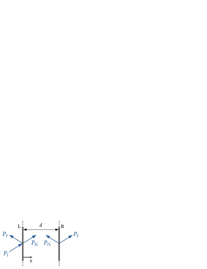
Figure 4: Double-leaf panel with leaves at a distance $d$ away from each other. Incident ($P_{i}$) and reflected ($P_{r}$) waves are formed before the left leaf (L), while transmitted waves ($P_{t}$) are formed after the right leaf (R). Standing waves ($P_{ti}$ and $P_{ri}$) are developed inside the cavity filled with fluid.

In this case, it is necessary to distinguish between the transverse displacements associated with panel leaves L and R, and also discriminate the standing waves $P_{ti}$ and $P_{ri}$, that are developed inside the fluid cavity, described by

$$u_{z}^{(\text{L})}(\mathbf{r},t) =e^{-\text{i}\omega t}\sum_{\mathbf{G}}\hat{u}_{z}^{(\text{L})}(\mathbf{G})e^{\text{i}(\mathbf{k}+\mathbf{G})\cdot\mathbf{r}}\,,$$ (41a)

$$u_{z}^{(\text{R})}(\mathbf{r},t) =e^{-\text{i}\omega t}\sum_{\mathbf{G}}\hat{u}_{z}^{(\text{R})}(\mathbf{G})e^{\text{i}(\mathbf{k}+\mathbf{G})\cdot\mathbf{r}}\,,$$ (41b)

$$P_{ti}(\mathbf{r},z,t) =e^{-\text{i}\omega t}\sum_{\mathbf{G}}\hat{P}_{ti}(\mathbf{G})e^{\text{i}(\mathbf{k}+\mathbf{G})\cdot\mathbf{r}}e^{\text{i}k_{za}(\mathbf{G})z}\,,$$ (41c)

$$P_{ri}(\mathbf{r},z,t) =e^{-\text{i}\omega t}\sum_{\mathbf{G}}\hat{P}_{ri}(\mathbf{G})e^{\text{i}(\mathbf{k}+\mathbf{G})\cdot\mathbf{r}}e^{-\text{i}k_{za}(\mathbf{G})z}\,.$$ (41d)

Following the same reasoning as in the previous section, we will begin by writing the fluid-structure coupling equations that allow to express the Fourier coefficients of the plane waves of interest.

Considering the continuity of accelerations (Eq. (20)) at the incident face of panel leaf L and at the transmitted face of panel leaf R, one has, respectively, the relations

$$\hat{P}_{r}(\mathbf{G}) =\frac{k_{z}}{k_{za}(\mathbf{G})}\hat{P}_{i}(\mathbf{G})+\frac{\text{i}\rho_{0}\omega^{2}}{k_{za}(\mathbf{G})}\hat{u}_{z}^{(\text{L})}(\mathbf{G})\,,$$ (42a)

$$\hat{P}_{t}(\mathbf{G}) =-\frac{\text{i}\rho_{0}\omega^{2}}{k_{za}(\mathbf{G})e^{\text{i}k_{za}(\mathbf{G})d}}\hat{u}_{z}^{(\text{R})}(\mathbf{G})\,.$$ (42b)

The standing waves can be related in an analogous way, considering the continuity of accelerations at the transmitted face of panel leaf L and incident face of panel leaf R, which leads to the the Fourier coefficients of the plane waves inside the acoustic cavity expressed as

$$\hat{P}_{ti}(\mathbf{G}) =\frac{\rho_{0}\omega^{2}}{2k_{za}(\mathbf{G})\sin(k_{za}(\mathbf{G})d)}\bigg{(}e^{-\text{i}k_{za}(\mathbf{G})d}\hat{u}_{z}^{(\text{L})}(\mathbf{G})-\hat{u}_{z}^{(\text{R})}(\mathbf{G})\bigg{)}\,,$$ (43a)

$$\hat{P}_{ri}(\mathbf{G}) =\frac{\rho_{0}\omega^{2}}{2k_{za}(\mathbf{G})\sin(k_{za}(\mathbf{G})d)}\bigg{(}e^{\text{i}k_{za}(\mathbf{G})d}\hat{u}_{z}^{(\text{L})}(\mathbf{G})-\hat{u}_{z}^{(\text{R})}(\mathbf{G})\bigg{)}\,.$$ (43b)

Equations (42) and (43) can now be coupled with the dynamic equations of both plates. The fluid loading on panel leaf L can be written as

$$q^{(\text{L})}(\mathbf{r},t)=P_{i}(\mathbf{r},z=0,t)+P_{r}(\mathbf{r},z=0,t)-P_{ti}(\mathbf{r},z=0,t)-P_{ri}(\mathbf{r},z=0,t)\,,$$ (44)

which can be combined with Eqs. (42) and (43) to derive an equation analogous to Eq. (25) for panel leaf L, which can be stated as

$$\sum_{\mathbf{G}_{j}}\bigg{[}\hat{D}^{(\text{L})}_{ij}f_{ij}-\omega^{2}\rho\hat{h}^{(\text{L})}_{ij}\bigg{]}\hat{u}_{z}^{(\text{L})}(\mathbf{G}_{j})+\frac{\rho_{0}\omega^{2}}{k_{za}(\mathbf{G}_{i})}\bigg{(}-\text{i}+\frac{1}{\tan(k_{za}(\mathbf{G}_{i})d)}\bigg{)}\hat{u}_{z}^{(\text{L})}(\mathbf{G}_{i})$$ (45)

$$-\frac{\rho_{0}\omega^{2}}{k_{za}(\mathbf{G}_{i})\sin(k_{za}(\mathbf{G}_{i})d)}\hat{u}_{z\mathbf{k}}^{(\text{R})}(\mathbf{G}_{i})=\bigg{(}1+\frac{k_{z}}{k_{za}(\mathbf{G}_{i})}\bigg{)}\hat{P}_{i}(\mathbf{G}_{i})\,,$$

where $\hat{D}^{(\text{L})}_{ij}$ and $\hat{h}^{(\text{L})}_{ij}$ refer to the Fourier coefficients of the flexural stiffness and thickness of panel leaf L computed for the reciprocal lattice vectors $\mathbf{G}_{i}-\mathbf{G}_{j}$.

Analogously, the fluid loading on panel leaf R can be written as

$$q^{(\text{R})}(\mathbf{r},t)=P_{ti}(\mathbf{r},z=d,t)+P_{ri}(\mathbf{r},z=d,t)-P_{t}(\mathbf{r},z=d,t)\,,$$ (46)

thus leading to an equation analogous to Eq. (45) for panel leaf R, which reads

$$\sum_{\mathbf{G}_{j}}\bigg{[}\hat{D}^{(\text{R})}_{ij}f_{ij}-\omega^{2}\rho\hat{h}^{(\text{R})}_{ij}\bigg{]}\hat{u}_{z}^{(\text{R})}(\mathbf{G}_{j})-\frac{\rho_{0}\omega^{2}}{k_{za}(\mathbf{G}_{i})\sin(k_{za}(\mathbf{G}_{i})d)}\hat{u}_{z}^{(\text{L})}(\mathbf{G}_{i})$$ (47)

$$+\frac{\rho_{0}\omega^{2}}{k_{za}(\mathbf{G}_{i})}\bigg{(}-\text{i}+\frac{1}{\tan(k_{za}(\mathbf{G}_{i})d)}\bigg{)}\hat{u}_{z}^{(\text{R})}(\mathbf{G}_{i})=0\,,$$

where $\hat{D}^{(\text{R})}_{ij}$ and $\hat{h}^{(\text{R})}_{ij}$ have the same meaning as in Eq. (45), but for panel leaf R.

Equations (45) and (47) can be organized in the form of a linear system as

$$\left[\begin{array}[]{cc}\widetilde{\mathbf{D}}^{(L)}+\mathbf{D}_{f}^{(d)}&\mathbf{D}_{f}^{(c)}\\ \mathbf{D}_{f}^{(c)}&\widetilde{\mathbf{D}}^{(R)}+\mathbf{D}_{f}^{(d)}\end{array}\right]\left\{\begin{array}[]{c}\hat{\mathbf{u}}_{z}^{(\text{L})}\\ \hat{\mathbf{u}}_{z}^{(\text{R})}\end{array}\right\}=\left\{\begin{array}[]{cc}\mathbf{f}\\ \mathbf{0}\end{array}\right\}\,,$$ (48)

where matrices $\widetilde{\mathbf{D}}^{(\text{L})}=\widetilde{\mathbf{K}}^{(\text{L})}-\omega^{2}\widetilde{\mathbf{M}}^{(\text{L})}$, $\widetilde{\mathbf{D}}^{(\text{R})}=\widetilde{\mathbf{K}}^{(\text{R})}-\omega^{2}\widetilde{\mathbf{M}}^{(\text{R})}$, are given by Eq. (30) for panel leaves L and R, respectively, the loading vector $\mathbf{f}$ is also given by the same equation, and diagonal matrices $\mathbf{D}_{f}^{(d)}$, $\mathbf{D}_{f}^{(c)}$ have elements given by

$$(\mathbf{D}_{f}^{(d)})_{ii} =\frac{\rho_{0}\omega^{2}}{k_{za}(\mathbf{G}_{i})}\bigg{(}-\text{i}+\frac{1}{\tan(k_{za}(\mathbf{G}_{i})d)}\bigg{)}\,,$$ (49)

$$(\mathbf{D}_{f}^{(c)})_{ii} =-\frac{\rho_{0}\omega^{2}}{k_{za}(\mathbf{G}_{i})\sin(k_{za}(\mathbf{G}_{i})d)}\,,$$

and the vectors of unknowns correspond to the Fourier coefficients for the displacements of panel leaves L and R (see Eq. (31)).

Interestingly, matrix $\mathbf{D}_{f}^{(d)}$ accounts for the fluid loading impedance at one side ($\mathbf{D}_{f}$/2, see Eq. (30)) and a contribution for the cavity impedance ($\tan$ term); meanwhile, the coupling between panel leaves L and R is provided by matrix $\mathbf{D}_{f}^{(c)}$. The form of Eq. (49) suggests that it can be easily extended for an arbitrary number of leaves.

4.3 Acoustic metrics

The sound power transmission coefficient ($\tau$) can be calculated for a given set of angles ($\varphi$, $\theta$) and angular frequency $\omega$ using [23]

$$\tau(\varphi,\,\theta,\,\omega)=\frac{\sum_{\mathbf{G}}|\hat{P}_{t}(\mathbf{G})|^{2}\,\text{Re}(k_{za}(\mathbf{G}))}{|\hat{P}_{i}|^{2}k_{z}}\,.$$ (50)

Thus, the sound transmission loss (STL) can be obtained using

$$\text{STL}(\varphi,\,\theta,\,\omega)=10\log\bigg{(}\frac{1}{\tau(\varphi,\,\theta,\,\omega)}\bigg{)}\,.$$ (51)

For the case of acoustic waves with oblique incidence angles, the diffuse power transmission coefficient ($\tau_{\text{d}}$) may be calculated using [46]

$$\tau_{\text{d}}(\theta,\,\omega)=\int_{0}^{\pi/2}\,\tau(\varphi,\,\theta,\,\omega)\,\sin 2\varphi\,d\varphi\,,$$ (52)

which, for the purpose of numerical evaluation, can be evaluated using angles between $0^{o}$ and $78^{o}$ [13]. This definition can also be used with Eq. (51) to express the diffuse STL as

$$\text{STL}_{\text{d}}(\theta,\,\omega)=10\log\bigg{(}\frac{1}{\tau_{d}(\theta,\,\omega)}\bigg{)}\,.$$ (53)

With the purpose of validating the PWE formulation, analytical expressions obtained from the literature are also presented. The analytical sound power transmission coefficient ($\tau_{\text{a}}$) for an infinite constant-thickness flat plate (and thus independent of $\theta$) with the same fluid on both sides can be calculated using [46]

$$\tau_{\text{a}}^{\text{s}}(\varphi,\,\omega)=\frac{(2\rho_{0}c_{0}\sec\varphi)^{2}}{(2\rho_{0}c_{0}\sec\varphi)^{2}+(\omega\rho h-(D/\omega)(k_{0}\sin\varphi)^{4})^{2}}\,,$$ (54)

which can be used in the place of the numerically obtained $\tau(\varphi,\,\theta,\,\omega)$ in Eq. (51) to calculate the analytical STL.

The frequency $f_{co}$ given by

$$f_{co}(\varphi)=\frac{1}{2\pi}\bigg{(}\frac{c_{0}}{\sin\varphi}\bigg{)}^{2}\sqrt{\frac{\rho h}{D}}\,,$$ (55)

is named coincidence frequency [13], and corresponds to the frequency at which the structural impedance for the plate is minimal for a given incidence angle ($\varphi$), causing a dip in the STL curve. For $\varphi=\pi/2$ this frequency becomes minimal, and is named critical frequency.

For the case of a double-leaf panel with plates of constant thickness, the power transmission coefficient is given by

$$\tau_{\text{a}}^{\text{d}}(\varphi,\,\omega)=\bigg{|}\frac{2\text{i}(\rho_{0}c_{0}\sec\varphi)^{2}\sin(k_{0}d\cos\varphi)}{(\text{i}\omega\rho h_{\text{L}}+z_{0})(\text{i}\omega\rho h_{\text{R}}+z_{0})\sin^{2}(k_{0}d\cos\varphi)+(\rho_{0}c_{0}\sec\varphi)^{2}}\bigg{|}^{2}\,,$$ (56)

where $z_{0}=\rho_{0}c_{0}\sec\varphi(1-\text{i}\cot(k_{0}d\cos\varphi))$ is a term associated with the cavity impedance and $h_{\text{L}}$ and $h_{\text{R}}$ are the thicknesses of the first and second leaves, respectively.

5 Optimisation problem

In the low-frequency range, a common solution to improve the STL consists of increasing the panel thickness. However, this is not the most economical solution, since it certainly implies more mass and the use of more material. Thus, the proposed objective here is to determine either an optimal thickness profile distribution or the inclusion of mass-spring resonators to achieve the maximum STL at a given frequency of interest. Thus, this optimisation objective can be stated as

$$\underset{\mathbf{d}}{\text{maximize}}\>\phi=\int_{\omega_{\min}}^{\omega_{\max}}\,\frac{1-e^{-\Delta\text{STL}(\omega)}}{1+e^{-\Delta\text{STL}(\omega)}}\,d\omega\,,$$ (57)

where $\Delta\text{STL}(\omega)=\text{STL}(\varphi=0,\omega)-\text{STL}_{\text{ref}}(\varphi=0,\omega)$ is the difference between the normal STL obtained for a set $\mathbf{d}$ of design variables and the reference STL computed for an initial constant-thickness plate, integrated over the frequency range $[\omega_{\min},\,\omega_{\max}]$. The set of design variables $\mathbf{d}$ may refer either to a plate thickness profile ($h_{n_{x},\,n_{y}}$, see Eq. (6)) or to a set of mass-spring resonators ($k_{p}$, $m_{p}$, $\mathbf{r}_{p}$, see Eq. (13)). The proposed integrand becomes $1$ for $\Delta\text{STL}\gg 0$ and $-1$ for $\Delta\text{STL}\ll 0$, which indicates an improvement (degradation) with respect to the original STL for sufficiently larger (smaller) values. It is important to notice that the incidence angle $\varphi=0$ does not contribute to the computation of the diffuse STL (Eqs. (52) and (53)), which must be verified to assess the improvement in performance in this case.

The definition of the constraints will depend on the case treated. Therefore, we will describe the thickness-varying plate without resonators case and the constant-thickness plate with resonators case separately hereafter.

5.1 Thickness-varying plate without resonators

Starting from Eq. (7), the plate thickness may be rewritten explicitly in terms of the $x$ and $y$ coordinates using Eq. (2) as

$$h(x,y)=\sum_{n_{y}}\sum_{n_{x}}\hat{h}_{n_{x},\,n_{y}}e^{\text{i}n_{x}(2\pi/L)x}e^{\text{i}n_{y}(2\pi/L)y}\,,$$ (58)

which presents a considerable reduction in the number of variables $\hat{h}_{n_{x},\,n_{y}}$ needed to describe the plate shape when assuming a symmetry of coefficients centered around $\hat{h}_{0,\,0}$, i.e., $\hat{h}_{n_{x},\,n_{y}}=\hat{h}_{n_{x},\,-n_{y}}=\hat{h}_{-n_{x},\,n_{y}}=\hat{h}_{-n_{x},\,-n_{y}}$.

The constraints on the plate thickness can be written as $h_{\min}\leq h(x,y)\leq h_{\max}$, where $h_{\min}$ and $h_{\max}$ are the minimum and maximum allowed values of plate thickness, respectively, which must hold true for $-L/2\leq\{x,\,y\}\leq L/2$. An additional constraint can be imposed to evaluate different plate thickness profiles that present the same mass per unit area. This can be achieved by setting a fixed mean value for the plate thickness, which means material addition implies in the same amount of material removal. Thus, this does not imply in an additional constraint, but in the removal of $\hat{h}_{0,\,0}$ from the list of optimisation variables, fixing it at the beginning of the optimisation process. This leaves us with the suitable boundaries of optimisation variables given by

$$-h_{\max}\leq\,\hat{h}_{n_{x},\,n_{y}}\leq h_{\max}\,,\forall\{n_{x},\,n_{y}\}\neq\{0,0\}\,.$$ (59)

The interested reader is referred to a thorough discussion on this approach [28].

5.2 Constant-thickness plate with resonators

For the case of the inclusion of resonators, some simplifications may be assumed to reduce the number of optimisation variables. First, by recalling that the medium is periodic, let us assume that the resonating structures are equally distributed through the unit cell. Thus, let us assume that the locations of the $p$-th resonator is uniquely determined by

$$x_{p}=-L/2+L_{r}n_{x}\,,y_{p}=-L/2+L_{r}n_{y}\,,$$ (60)

where $L_{r}=L/(n_{rd}+1)$ is the spacing between consecutive resonators in a given direction $x$ or $y$ (figure 5), where the total number of resonators is given by $n_{r}=n_{rd}^{2}$, and $0\leq\{n_{x},\,n_{y}\}\leq n_{rd}$.

Figure 5: Unit cell with dimensions $L\times L$ with evenly spaced resonators at a distance $L_{r}$ from each other.

It is also reasonable to assume that the mass of each resonator is constant, i.e., $m_{p}=\Delta m/n_{r}$, $\forall p$, where $\Delta m$ is the total added mass of the resonators. To keep the same base of comparison between distinct designs, we also restrict the total amount of added mass to keep the same mass per unit cell. This can be achieved by setting

$$\Delta m=\rho L^{2}\Delta h\,,$$ (61)

where $\Delta h=h_{0}-h$ is the thickness variation of the plate, calculated as the difference between the current thickness $h$ and the initial thickness $h_{0}$. Thus, for a plate with constant thickness $h<h_{0}$, the mass of the resonators can be determined.

The stiffness $k_{p}$ of each resonator can be set by properly choosing their resonant frequency, $\omega_{p}$, i.e., $k_{p}=m_{p}\omega_{p}^{2}$, for $p=\{1,2,\,\dots,n_{r}\}$. The resonant frequency of each resonator can be obtained by sampling a two-dimensional function of a continuous stiffness written as

$$\omega_{p}=\omega_{c}(x_{p},\,y_{p})\,$$ (62)

where the continuous function $\omega_{c}(x,y)$ can be expressed in the same way as Eq. (58), i.e.,

$$\omega_{c}(x,y)=\sum_{n_{y}}\sum_{n_{x}}\hat{\omega}_{n_{x},\,n_{y}}e^{\text{i}n_{x}(2\pi/L)x}e^{\text{i}n_{x}(2\pi/L)y}\,.$$ (63)

Expressing a continuous resonant frequency function in such a manner may present great advantages for a large number of resonators, since the $\omega_{c}(x,y)$ function may be sampled at will without increasing the number of design variables. The lower and upper bounds of $\omega_{c}(x,y)$ may be selected as

$$\omega^{(r)}_{\min}\leq\omega_{c}(x,y)\leq\omega^{(r)}_{\max}\,,$$ (64)

where $\omega^{(r)}_{\min}$ and $\omega^{(r)}_{\max}$ refer to the minimum and maximum frequencies of interest, respectively. The constraints on the stiffness function can be set in an analogous way as used for thickness, i.e., Eq. (59), using

$$\omega^{(r)}_{\min}\leq\, \hat{\omega}_{0,0}\,\leq\omega^{(r)}_{\max}\,,$$ (65a)

$$-\omega^{(r)}_{\max}\leq\, \hat{\omega}_{n_{x},\,n_{y}}\leq\omega^{(r)}_{\max}\,,\forall\{n_{x},\,n_{y}\}\neq\{0,0\}\,.$$ (65b)

6 Results

The STL computations are performed using the numeric PWE-based formulations presented in Section 4 for both the thickness-varying plates (PCs) and the constant-thickness plate with included mass-spring resonators (MMs). The results are computed using the material properties of aluminium (Young’s modulus $E=70$ GPa, Poisson’s coefficient $\nu=0.3$, and mass density $\rho=2700$ kg/m³). The mean plate thickness is chosen as $\overline{h}=3$ mm and this is the constant value for analytical formulations. For these material properties and plate thickness, the critical frequency (Eq. (55)) is $4$ kHz. For the maximum frequency of $1$ kHz (well below the critical frequency), the maximum flexural wave speed (Eq. (4)) is $170$ m/s, which corresponds to a minimum wavelength $\lambda_{\min}=170$ mm and a relation $\overline{h}/\lambda_{\min}\approx 1/57$. For the PC plate, the thickness remains in the range $[h_{\min},\,h_{\max}]=[1,\,5]$ mm. A square lattice of length $L=40h_{\max}=200$ mm is also considered to ensure a surface that has a smooth variation and allows to disregard deviations in the fluid-structure interaction with respect to the plate mean thickness. For the double-leaf configuration, leaves are separated by $d=1.5h_{\max}=7.5$ mm. The surrounding fluid is air at $20^{o}$C, with a sound speed $c_{0}=340$ m/s and mass density $\rho_{0}=1.2$ kg/m³. The PWE-based numerical method for computing the STL uses $n_{G}=169$ plane waves ($N_{\max}=6$). For the optimisation process, a total of $28$ parameters is used ($-6\leq\{n_{x},\,n_{y}\}\leq 6$ with symmetric parameters, see Section 5).

6.1 Comparison between analytical and numerical results

We start by comparing the STLs obtained for both normal ($\varphi=0^{o}$) and diffuse incidences ($0^{o}\leq\varphi\leq 78^{o}$ for the computation of Eq. (52)) for both the analytical and PWE-based numerical solutions (Eqs. (28)). Figure 6 shows an excellent agreement between both. While no differences are noticed for the single-leaf case (figure 6a), a small deviation is noticed for the double-leaf diffuse case (figure 6b), where the PWE approach presents slightly different STL values above $800$ Hz. An STL dip corresponding to the mass-air-mass resonance of the double-leaf system is also noticed at $340$ Hz.

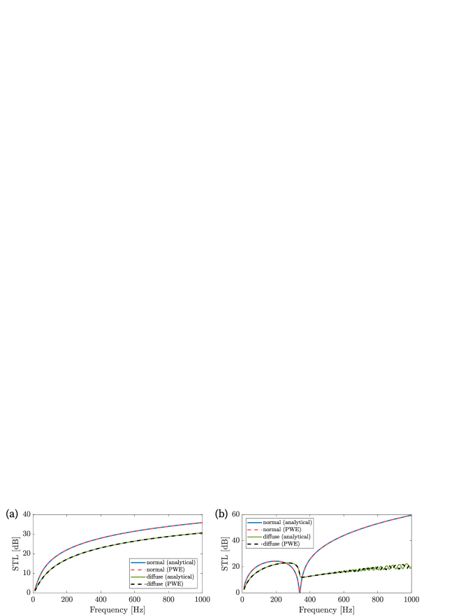
Figure 6: Computed STLs for the (a) single-leaf and (b) double-leaf panels. The curves indicate the results for the normal and diffuse incidence cases, comparing both analytical and PWE approaches.

The following section presents the optimisation results obtained for a one-octave frequency range centred at $350$ Hz (chosen close to the STL dip for the double-leaf initial case), i.e., from $248$ Hz to $495$ Hz.

6.2 Optimisation results

The results for the PC case consider a fixed mean thickness of $h_{0}=\overline{h}=3$ mm. For the analysed frequency range, the obtained optimal thickness profile indicates a large area with the maximum thickness and a circular thickness reduction at the centre of the unit cell ($h_{\max}=5$ mm and $h_{\min}=1$ mm, respectively, see figures 7a and 7b). The computed normal incidence STL for the single-leaf case (figure 7c) presents a large increase of the STL curve inside the frequency range of interest ($75.0$ dB at $464$ Hz), followed by a decrease outside this range ($0.01$ dB at $532$ Hz). The points of maximum and minimum correspond to the displacement profiles shown, for each case, using equivalent colour coding for the absolute displacement: an increase in the STL is achieved by a overall decrease in displacements of the unit cell (anti-resonance behaviour, represented in the green square), while a decrease in the STL curve is associated with an increase in the displacement of the region with the smallest thickness (resonance behaviour, represented in the purple square). It is also interesting to notice that no degradation is noticed before the upper limit of the optimisation frequency range. Very similar results are obtained when analysing other frequency ranges (see Supplementary Material).

For the double-leaf case, a similar result is obtained (figure 7d), although, in this case, two anti-resonances ($87.0$ dB at $427$ Hz and $85.0$ dB at $506$ Hz) and two resonances ($0.29$ dB at $534$ Hz and $0.01$ dB at $562$ Hz) are present, which arises due to the combination of unit cell displacements in anti-phase (AP) and in-phase (P) combinations (shown with the same colour coding for proper comparison). Thus, an overall increase of performance is observed in the frequency range of interest. However, the STL dip due to the mass-air-mass resonance is still present.

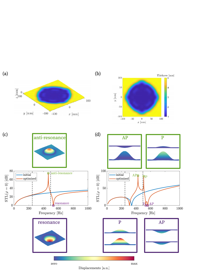
Figure 7: Results for the PC panel considering normal incidence. (a,b) Optimised unit cell in the single-leaf case and (c) corresponding improvement in the STL within the target frequency range due to an anti-resonance (green square), with a decrease of the STL outside the target frequency range due to resonance (purple square). (d) Same for the double-leaf case with optimised unit cell with anti-phase (AP) and in-phase (P) anti-resonances (green squares) and resonances (purple squares).

However, one must recall that, for the normal incidence, the in-plane wavenumbers are zero (i.e., $k_{x}=k_{y}=0$), and thus the characteristics observed in the STL for normal incidence are not necessarily associated with any particular in-plane wave propagation attenuation mechanisms. Thus, to correlate the STLs with the plate structural behaviour, we plot the dispersion relation for the PC plate along with some noticeable wave modes (figure 8a), which shows partial band gaps are opened due to Bragg scattering ($187.1$ Hz – $215.3$ Hz and $537.4$ Hz – $582.0$ Hz for the $\Gamma$X direction, $346.3$ Hz – $407.5$ Hz for the XM region, and $756.7$ Hz – $804.1$ Hz for the $\Gamma$M directions, respectively). Some wave modes associated with these band gaps may present the same displacement profiles as the resonance points of the normal incidence, as in the case of the wave modes indicated as (i), (ii), and (iv) (red squares), while other wave modes, such as the one indicated by (iii) (blue square), do not present the same displacement profile as a localized STL resonance. Thus, wave modes (i), (ii), and (iv) may be excited by acoustic impinging waves.

To confirm this correlation, the results for oblique ($\varphi\neq 0$) incident waves using the values $\varphi=\{0,\,5^{o},\,\dots,\,85^{o}\}$ are plotted for the directions $\theta=0$ and $\theta=\pi/4$ and shown with the partial band gaps calculated for the direction $\Gamma$X and $\Gamma$M, respectively. For the $\Gamma$X direction ($\theta=0$, figure 8b), resonances are easily noticed both above and below the second band gap, which correspond to the wave modes (i) and (ii) excited at different frequencies. For the $\Gamma$M direction ($\theta=\pi/4$, figure 8c), this is noticeable for the wave mode (iv), just below the shown band gap. For frequencies immediately above the band gap the STL remains unaffected, since the associated wave mode (iii) is not excited by the incident acoustic wave. Thus, the immediate effect of the opened partial band gaps is to impede the formation of resonances in their interior, although anti-resonances may still be present. The consequence of these characteristics is noticed when analysing the diffuse STLs for the single- (figure 8d) and double-leaf cases (figure 8e). Although sharp peaks may be introduced in the diffuse STL for both cases, the target frequency range may also present ranges where degradation occurs.

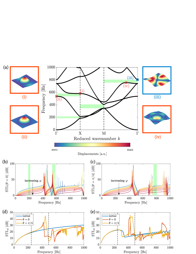
Figure 8: Results for the PC panel under oblique and diffuse incidences. (a) Dispersion diagram for the optimised unit cell with partial band gaps (green regions) associated with wave modes (i), (ii), (iv) (red squares), and (iii) (blue square). STL considering oblique incidence angles for directions (b) $\theta=0$ and (c) $\theta=\pi/4$. STL for diffuse incidence for (d) single- and (e) double-leaf cases.

For the MM case, the resonators are included keeping a constant unit cell mass. The plate thickness is now reduced to $h_{\min}$, while the mass corresponding to the thickness variation, $\Delta m=216$ g, is added in the form of resonators, with resonating frequencies in the range $[\omega^{(r)}_{\min},\,\omega^{(r)}_{\max}]/2\pi=[0.001,\,10]$ kHz, thus allowing the resonators to vary over a wide frequency range. The optimisation process is performed for the cases of a single resonator and also multiple distributed resonators (chosen for a total number of $25$, in this case).

We begin by analysing the resonator distribution obtained by each optimisation and their corresponding dispersion relations. For the single resonator case, a resonant frequency of $518$ Hz is indicated by the optimisation process (figure 9a), which results in a dispersion diagram with a full band gap (i.e., for all propagation directions) in the $38.3$ Hz – $60.5$ Hz frequency range (figure 9b). The inclusion of a resonator with a large mass results in the flattening of the first flexural branch [42], which is associated with a wave mode showing large displacements at the resonator (wave mode (i) at $38.3$ Hz, red square) and a wave mode with pronounced displacements at the plate (wave mode (ii) at $60.5$ Hz, blue square).

For the case of multiple resonators, the optimisation indicates one resonator with a higher frequency ($819$ Hz) and several resonators with lower frequencies ($368$ Hz – $557$ Hz range, figure 9c), with an appreciable superposition over the target optimisation frequency range. The resulting band diagram presents multiple flat bands (figure 9d), which represent zero group velocity branches typical of locally resonant wave modes. Although this design presents a wide effective band gap (around $440$ Hz – $785$ Hz) this may not necessarily translate into an effective STL gain, since, although some wave modes are associated with the displacement of resonators (wave mode (iii) at $438.7$ Hz, blue square), several wave modes are still associated with large plate displacements (e.g., wave mode (iv) at $664.9$ Hz, red square).

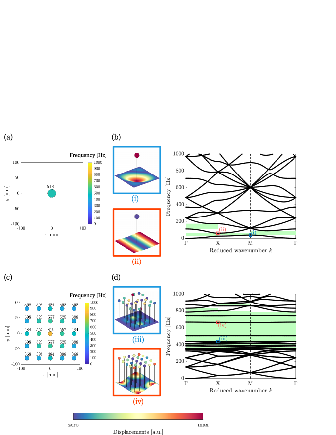
Figure 9: Optimisation results for the MM panel. (a) Single-resonator result with (b) dispersion diagram showing band gaps (green patches) and wave modes (i) and (ii) showing predominantly resonator (blue square) or plate displacements (red square). (c) Multiple-resonator result with (d) dispersion diagram showing several zero group velocity branches, opening large band gaps and wave modes (iii) and (iv).

The resulting STLs for the single-leaf under normal incidence are presented with the corresponding STLs for the constant-thickness plates with the mean thickness values of $\overline{h}$ (initial value) and $h_{\min}$ (on which the resonators are embedded) in figure 10a. The resulting STL is richer in dynamic behaviour when compared with the equivalent results for the PC. Examples of anti-resonance (green squares) and resonance behaviour (purple squares) are exemplified by S1 – S4 (for the single resonator MM) and M1 – M3 (for the multiple-resonator MM). Each displacement profile uses a colour scale normalized with respect to its maximum displacement for the purpose of comparing the plate and resonator displacements, while using the same out-of-plane displacement scaling factor.

The single resonator MM presents an STL similar to the plate with thickness $h_{\min}$, with deviations exemplified by the points labelled as S1 – S4. Increases in this STL ($46.7$ dB at $67$ Hz for S1 and $51.4$ dB for $358$ Hz for S3, respectively) are associated with an overall reduction in the plate displacement, while decreases in the STL ($\approx 0$ dB at $110$ Hz for S2 and $0.03$ dB at $367$ Hz for S4) are associated with smaller resonator displacements and larger plate displacements. The resulting STL does not achieve an improvement over the desired optimisation frequency range. The multiple-resonator MM design is able to achieve a significantly higher STL. As in the PC design, no degradation is noticed in the STL until the upper edge of the optimisation frequency range. Analogously to the single resonator MM design, the anti-resonances show a large displacement of the resonator masses and small plate displacements (e.g., $67.3$ dB at $409$ Hz for M1 and $75.7$ dB at $432$ Hz for M2), while for the resonances, this behaviour is the opposite (e.g., $\approx 0$ dB at $664$ Hz for M3).

For the multiple-resonator MM case, the wavelength-independence of the flat bands in the corresponding dispersion diagram (figure 9d) also facilitate relating the wave modes with the anti-resonances and resonances: the anti-resonance M2 presents a frequency very similar to wave mode (iii) and the resonance M3 similar to wave mode (iv). Thus, although a wide band gap does exist and may be beneficial for structural applications, its effectiveness in improving the STL is conditioned to the shapes of the wave modes, which may be excited by impinging acoustic waves. Also, unlike the single resonator design, the use of several diverse resonators is able to achieve STL improvements in a broader frequency range, thus overcoming the shortcomings of the narrow frequency range influence of the resonant behaviour typically associated with single-frequency resonators.

The computed STLs using diffuse incidence for the single-leaf case are presented for the single- and multiple-resonator MM designs for the directions $\theta=0$ (figure 10b) and $\theta=\pi/4$ (figure 10c). The resulting behaviour is very similar to the normal incidence case, although with smaller improvements in the STL. Also, it is interesting to notice that the wavelength independence of such locally-resonant based designs is insensitive to variations in the angle of incidence of the acoustic excitation, which implies an improved robustness for practical applications.

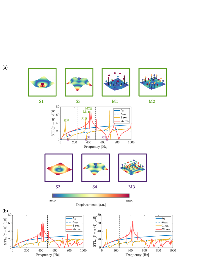
Figure 10: Computed STLs for the single-leaf MM panel designs. (a) Normal-incidence case; improvements in the STLs are associated with localized resonator displacements (green squares, S1, S3, M1, and M2), while degradation occurs due to large plate displacements (purple squares, S2, S4, and M3), both related with the wave modes (figures 9b and 9d, (i)–(iv)). (b) Diffuse-incidences cases (directions $\theta=0$ and $\theta=\pi/4$) for minimum and maximum panel thickness, single-resonator, and multiple-resonator designs. The thinner plate ($h_{\min}$) is used for the attachment of resonators.

The obtained results for both the single- and multiple-resonator double-leaf MM designs under normal incidence (figure 11a) presents both STLs following the overall behaviour of the thinner plate, with the main characteristic of shifting the mass-air-mass resonant frequency to higher values, removing it from the optimisation frequency range. However, while the multi-resonator MM design introduces a single dip in the STL, the single-resonator design introduces two new dips at the vicinity of the previously existing one. Despite local deviations, the overall behaviour in the optimisation frequency range is nearly constant, presenting an overall degradation of the STL with respect to the thicker plate. A similar behaviour is observed for the double-leaf diffuse incidence case (figure 11b, shown for $\theta=0$ and $\theta=\pi/4$), thus not presenting any justifiable gains over the original, thicker plate.

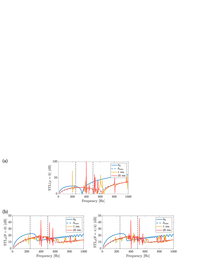
Figure 11: Computed STLs for the double-leaf MM panel configuration. (a) Normal and (b) diffuse incidence cases for minimum and maximum panel thickness, single-resonator, and multiple-resonator designs.

We have also performed an optimisation considering the possibility of changing both the thickness profile and resonator distribution, allowing the mean thickness to change while adding the corresponding mass reduction in the form of distributed resonators. The results yielded practically the same design as in the PC case (with deviations in the thickness parameters smaller than $1\times 10^{-5}$) with zero resonator masses). This result is partially owed to the form of the integrand in the optimisation metric (see Eq. (57)), which quickly converges to unity for sufficiently large improvements in the STL, thus favouring smaller STL improvements in wider frequency ranges (typical of PC designs) over large STL improvements in narrow frequency ranges (typical of MM designs).

7 Conclusions

Inspired by the locally resonant structures present in butterfly and moth wings and based on our previously work on thickness-varying plates for structural applications, we have investigated the utilization of these structures for acoustic insulation systems using both single- and double-leaf configurations.

With the proposed optimisation scheme, we obtained a PC plate with a thickness profile that presents an improvement in the STL under normal incidence, for both single- and double-leaf configurations, based on the anti-resonance behaviour of the unit cell. However, its dispersion diagram reveals that several wave modes may be excited by acoustic impinging waves outside of existing band gaps, thus degrading its performance for diffuse incidence cases.

The same optimisation procedure allows to obtain MMs constituted by plates with a reduced thickness and distributed resonators, while keeping the same unit cell mass. In this case, we obtained an optimised unit cell which produces wide band gaps associated with zero group velocity branches, with wave modes predominantly associated with either resonator or plate displacements. The use of multiple resonators with smaller masses achieves a superior STL performance when compared with a single resonator with a large mass, which is achieved by the excitation of the wave modes yielded by the different combinations of resonator displacements, thus obtaining improvements over a wider frequency range. The resulting STLs present similar behaviours for both normal and diffuse incidences, in contrast with the PC designs. For the double-leaf case, however, no real gains are achieved, since the resulting systems present a behaviour similar to that of a thinner plate.

In view of such results, it is clear that MM-based designs perform in a remarkably more robust manner for both normal and diffuse incidence cases for single-leaf configurations, due to their independence of the associated wavelength for the incident acoustic waves. These observations may also indicate why evolutionary pressure has led to the specialization of butterfly and moth wing structures in such a manner. The proposed PC-based designs, however, remain as interesting options when addressing normally-incident waves for both single- and double-leaf configurations.

This article has no additional data.

VFDP caried out the methodology, software, investigation, and writing of the original draft. NMP provided the computational resources, acquisition of funding, and performed the review of the manuscript. JRFA conceived and designed the study, performed the review of the manuscript, and overall supervision. All auhtors read and approved the manuscript.

The authors declare that they have no competing interests.

VFDP and NMP are supported by the EU H2020 FET Open “Boheme” grant No. 863179. JRFA thanks Conselho Nacional de Desenvolvimento Científico e Tecnológico (CNPq), Brazil, grant 305293/2021-4, and Fundação de Amparo à Pesquisa do Estado de São Paulo (FAPESP), Brazil, grant 2018/15894-0.

References

- [1] Barron RF. 2002 Industrial Noise Control and Acoustics. CRC Press.
- [2] Cremer L, Heckl M. 1967 Körperschall: physikalische Grundlagen und technische Anwendungen. Springer.
- [3] Ginn KB. 1978 Architectural Acoustics. Brüel & Kjær.
- [4] Doutres O, Dauchez N. 2005 Characterisation of porous materials viscoelastic properties involving the vibro-acoustical behaviour of coated panels .
- [5] Doutres O, Dauchez N, Génevaux JM. 2007 Porous layer impedance applied to a moving wall: Application to the radiation of a covered piston. The Journal of the Acoustical Society of America 121, 206–213.
- [6] Craik R, Smith R. 2000 Sound transmission through double leaf lightweight partitions part i: airborne sound. Applied Acoustics 61, 223–245.
- [7] Tadeu A, António J, Mateus D. 2004 Sound insulation provided by single and double panel walls: a comparison of analytical solutions versus experimental results. Applied Acoustics 65, 15–29.
- [8] Shen Z, Neil TR, Robert D, Drinkwater BW, Holderied MW. 2018 Biomechanics of a moth scale at ultrasonic frequencies. Proceedings of the National Academy of Sciences 115, 12200–12205.
- [9] Clare EL, Holderied MW. 2015 Acoustic shadows help gleaning bats find prey, but may be defeated by prey acoustic camouflage on rough surfaces. Elife 4, e07404.
- [10] Neil TR, Shen Z, Robert D, Drinkwater BW, Holderied MW. 2020 Moth wings are acoustic metamaterials. Proceedings of the National Academy of Sciences 117, 31134–31141.
- [11] Yang M, Sheng P. 2017 Sound absorption structures: From porous media to acoustic metamaterials. Annual Review of Materials Research 47, 83–114.
- [12] Long M. 2005 Architectural Acoustics. Elsevier.
- [13] Fahy FJ, Gardonio P. 2007 Sound and Structural Vibration: Radiation, Transmission and Response. Elsevier.
- [14] Wang T, Sokolinsky VS, Rajaram S, Nutt SR. 2005 Assessment of sandwich models for the prediction of sound transmission loss in unidirectional sandwich panels. Applied Acoustics 66, 245–262.
- [15] Sui N, Yan X, Huang TY, Xu J, Yuan FG, Jing Y. 2015 A lightweight yet sound-proof honeycomb acoustic metamaterial. Applied Physics Letters 106, 171905.
- [16] Zhang Z, Du Y. 2017 Sound insulation analysis and optimization of anti-symmetrical carbon fiber reinforced polymer composite materials. Applied Acoustics 120, 34–44.
- [17] Romero-Garcia V, Hladky-Hennion AC. 2019 Fundamentals and applications of acoustic metamaterials: From seismic to radio frequency. John Wiley & Sons.
- [18] Kushwaha MS, Halevi P, Martinez G, Dobrzynski L, Djafari-Rouhani B. 1994 Theory of acoustic band structure of periodic elastic composites. Physical Review B 49, 2313.
- [19] Liu Z, Zhang X, Mao Y, Zhu Z Y Y Yang, Chan CT, Sheng P. 2000 Locally resonant sonic materials. Science 289, 1734–1736.
- [20] Goffaux C, Sánchez-Dehesa J, Yeyati AL, Lambin P, Khelif A, Vasseur J, Djafari-Rouhani B. 2002 Evidence of Fano-like interference phenomena in locally resonant materials. Physical review letters 88, 225502.
- [21] Claeys CC, Sas P, Desmet W. 2014 On the acoustic radiation efficiency of local resonance based stop band materials. Journal of Sound and Vibration 333, 3203–3213.
- [22] Claeys C, Deckers E, Pluymers B, Desmet W. 2016 A lightweight vibro-acoustic metamaterial demonstrator: Numerical and experimental investigation. Mechanical systems and signal processing 70, 853–880.
- [23] Xiao Y, Wen J, Wen X. 2012 Sound transmission loss of metamaterial-based thin plates with multiple subwavelength arrays of attached resonators. Journal of Sound and Vibration 331, 5408–5423.
- [24] Oudich M, Zhou X, Badreddine Assouar M. 2014 General analytical approach for sound transmission loss analysis through a thick metamaterial plate. Journal of Applied Physics 116, 193509.
- [25] Van Belle L, Claeys C, Deckers E, Desmet W. 2019 The acoustic insulation performance of infinite and finite locally resonant metamaterial and phononic crystal plates. In MATEC Web of Conferences, volume 283, p. 09003. EDP Sciences.
- [26] Sorokin VS. 2016 Effects of corrugation shape on frequency band-gaps for longitudinal wave motion in a periodic elastic layer. The Journal of the Acoustical Society of America 139, 1898–1908.
- [27] Pelat A, Gallot T, Gautier F. 2019 On the control of the first Bragg band gap in periodic continuously corrugated beam for flexural vibration. Journal of Sound and Vibration 446, 249–262.
- [28] Dal Poggetto VF, Arruda JRdF. 2021 Widening wave band gaps of periodic plates via shape optimization using spatial Fourier coefficients. Mechanical Systems and Signal Processing 147, 107098.
- [29] Kinsler LE, Frey AR, Coppens AB, Sanders JV. 1999 Fundamentals of Acoustics.
- [30] Kang YJ, Bolton JS. 1996 A finite element model for sound transmission through foam-lined double-panel structures. The Journal of the Acoustical Society of America 99, 2755–2765.
- [31] Yang Y, Mace BR, Kingan MJ. 2017 Prediction of sound transmission through, and radiation from, panels using a wave and finite element method. The Journal of the Acoustical Society of America 141, 2452–2460.
- [32] Dal Poggetto VF, Serpa AL. 2021 Flexural wave band gaps in a ternary periodic metamaterial plate using the plane wave expansion method. Journal of Sound and Vibration 495, 115909.
- [33] Dal Poggetto VF, Serpa AL. 2020 Elastic wave band gaps in a three-dimensional periodic metamaterial using the plane wave expansion method. International Journal of Mechanical Sciences 184, 105841.
- [34] Beli D, Arruda JRF, Ruzzene M. 2018 Wave propagation in elastic metamaterial beams and plates with interconnected resonators. International Journal of Solids and Structures 139, 105–120.
- [35] Li H, Jiang L, Jia W, Qiang H, Li X. 2009 Genetic optimization of two-dimensional photonic crystals for large absolute band-gap. Optics Communications 282, 3012–3017.
- [36] Doosje M, Hoenders BJ, Knoester J. 2000 Photonic bandgap optimization in inverted FCC photonic crystals. Journal of the Optical Society of America B 17, 600–606.
- [37] Bin J, Wen-Jun Z, Wei C, An-Jin L, Wan-Hua Z. 2011 Improved plane-wave expansion method for band structure calculation of metal photonic crystal. Chinese Physics Letters 28, 034209.
- [38] Ventsel E, Krauthammer T. 2001 Thin Plates and Shells: Theory, Analysis, and Applications. CRC Press.
- [39] Leissa AW. 1969 Vibration of Plates. NASA SP. Scientific and Technical Information Division, National Aeronautics and Space Administration.
- [40] Torrent D, Mayou D, Sánchez-Dehesa J. 2013 Elastic analog of graphene: Dirac cones and edge states for flexural waves in thin plates. Physical Review B 87, 115143.
- [41] Miranda Jr EJP, Nobrega ED, Ferreira AHR, Dos Santos JMC. 2019 Flexural wave band gaps in a multi-resonator elastic metamaterial plate using Kirchhoff-Love theory. Mechanical Systems and Signal Processing 116, 480–504.
- [42] Xiao Y, Wen J, Wen X. 2012 Flexural wave band gaps in locally resonant thin plates with periodically attached spring–mass resonators. Journal of Physics D: Applied Physics 45, 195401.
- [43] Haslinger SG, Movchan NV, Movchan AB, Jones IS, Craster RV. 2017 Controlling flexural waves in semi–infinite platonic crystals with resonator–type scatterers. The Quarterly Journal of Mechanics and Applied Mathematics 70, 216–247.
- [44] Strang G. 1988 Linear Algebra and Its Applications. Harcourt, Brace, Jovanovich, Publishers.
- [45] Hsu HP. 1967 Fourier Analysis. Simon & Schuster.
- [46] Hambric SA, Sung SH, Nefske DJ. 2016 Engineering Vibroacoustic Analysis: Methods and Applications. John Wiley & Sons.