Two new families of fourth-order explicit exponential Runge–Kutta methods with four stages for stiff or highly oscillatory systems

Abstract

In this paper, two new families of fourth-order explicit exponential Runge–Kutta methods with four stages are studied for solving stiff or highly oscillatory systems $y^{\prime}(t)+My(t)=f(y(t))$. By comparing the Taylor expansions of numerical and exact solutions, we derive the order conditions of these new explicit exponential methods, which are exactly identical to the order conditions of the classical explicit Runge–Kutta methods, and these exponential methods reduce to the classical Runge–Kutta methods once $M\rightarrow\mathbf{0}$. Furthermore, we analyze the linear stability properties and the convergence of these new exponential methods in detail. Finally, several numerical examples are carried out to illustrate the accuracy and efficiency of these new exponential methods when applied to the stiff systems or highly oscillatory problems than standard exponential integrators.

Mathematics Subject Classification (2000): 65L05, 65L06

1 Introduction

The classical Runge–Kutta (RK) methods are extensively recognized by researchers and engineers for its simple idea and concise expression [5, 23, 30, 34, 36], and exponential Runge–Kutta (EKR) methods as an extension of standard RK methods which have been received a lot of attention (see, e.g., [7, 18, 19, 20, 23, 24, 25, 28, 29]). Normally, the coefficients of exponential integrators are exponential functions of the underlying matrix in the literature, this fact means that the implementation of these exponential methods needs to rely heavily on the evaluations of matrix exponentials. In order to reduce the computational cost, two new kinds of ERK methods up to order three were formulated and studied in [33]. As a sequel to this work, we study two new families of the fourth-order explicit ERK methods with four stages for stiff or highly oscillatory systems in this paper, which are termed modified and simplified versions of fourth-order explicit ERK integrators, respectively. It is noted that the coefficients of these fourth-order ERK methods are real constants, which are different from standard exponential integrators [21], then the computation of matrix exponentials is not needed.

In this paper, we pay attention to initial value problems of ordinary differential equations

$$\left\{\begin{array}[]{l}y^{\prime}(t)+My(t)=f(y(t)),\quad t\in[t_{0},t_{\rm end}],\cr\vskip 2.84526pt\cr y(t_{0})=y_{0},\end{array}\right.$$ (1)

where the matrix $M\in\mathbb{R}^{m\times m}$ is a symmetric positive definite or skew-Hermitian with eigenvalues of large modulus. Problems of the form (1) arise frequently in a variety of applied science such as quantum mechanics, flexible mechanics, and semilinear parabolic problems. In general, the equivalent form of (1) is presented by

$$\left\{\begin{array}[]{l}\displaystyle y^{\prime}(t)=g(y(t)),\quad t\in[t_{0},t_{\rm end}],\cr\vskip 2.84526pt\cr y(t_{0})=y_{0},\end{array}\right.$$ (2)

with $g(y)=-My(t)+f(y(t))$, and many practical numerical methods [11, 27, 31, 32, 35] have been presented for (1) or (2) in the literature. It is well known that the approximation of matrix-vector products with the exponential or a related function have been well developed (see, e.g., [4, 17]), and exponential integrators have extensive applications. In particular, for stiff systems, exponential integrators have distinguished advantages which can exactly integrate the linear equation $y^{\prime}(t)+My(t)=0$ in comparison with non-exponential integrators. The main idea of exponential integrators is primarily concerned with the use of Volterra integral equation

$$y(t_{0}+h)=e^{-hM}y(t_{0})+h\int_{0}^{1}e^{-(1-\tau)hM}f(y(t_{0}+h\tau))d\tau,$$ (3)

also termed the variation-of-constants formula. We also notice that Hochbruck et al. [19] have formulated ERK integrators based on the stiff-order conditions (comprise the classical order conditions). However, as stated by Berland et al. in [3], the stiff-order conditions are relatively strict. It is true that the fourth-order (stiff) ERK method (12) with five stages was proposed in [19], which is based on the stiff-order conditions in a weak form. Therefore, our study is related to the classical order conditions.

This paper is devoted to construct two new families of fourth-order (non-stiff) explicit exponential methods with four stages for solving the problems (1), which have the lower computational cost than the standard fourth-order exponential integrators. The order conditions of two novel proposed methods are derived in detail. It turns out that the order conditions of the new methods are equivalent to the order conditions of the classical explicit RK methods, which implies that the coefficients of classical RK methods can be straightforwardly used to construct the fourth-order explicit exponential methods in this paper.

The outline of the paper is as follows. In Section 2, we investigate and present the order conditions of the modified version of fourth-order explicit ERK methods. The simplified version of explicit ERK integrators of order four is formulated in Section 3. We analyze the linear stability properties and derive the convergence of our explicit ERK methods in Section 4, repectively. The numerical results present the accuracy and efficiency of our new explicit fourth-order ERK integrators, when applied to the averaged system in wind-induced oscillation, the Hénon-Heiles Model, the Allen-Cahn equation, the sine-Gorden equation and the nonlinear Schrödinger equation in Section 5. The concluding remarks are included in the last section.

2 A modified version of fourth-order explicit ERK methods

In order to reduce the computational cost of standard ERK methods, the internal stages and update of the modified version of ERK methods inherit and modify the form of classical RK methods, respectively.

Definition 2.1

([33]) An $s$-stage modified version of exponential Runge–Kutta (MVERK) method for the numerical integration (1) is defined as

$$\left\{\begin{array}[]{l}\displaystyle Y_{i}=y_{0}+h\sum\limits_{j=1}^{s}a_{ij}(-MY_{j}+f(Y_{j})),\ i=1,\ldots,s,\cr\vskip 11.38109pt\cr\displaystyle y_{1}=e^{-hM}y_{0}+h\sum\limits_{i=1}^{s}b_{i}f(Y_{i})+w_{s}(z),\end{array}\right.$$ (4)

where $a_{ij}$, $b_{i}$ are real constants for $i,j=1,\ldots,s$, $Y_{i}\approx y(t_{0}+c_{i}h)$ for $i=1,\ldots,s$, and $w_{s}(z)$ depends on $h$, $M$, and $w_{s}(z)\rightarrow 0$ when $M\rightarrow\mathbf{0}$.

In [33], it is clearly indicated that $w_{s}(z)$ is independent of matrix-valued exponentials. In fact, the $w_{s}(z)$ is also related to the term $f(\cdot)$ and initial value $y_{0}$, and the MVERK methods with the same order share the same $w_{s}(z)$. In particular, when we consider the MVERK method with order one, then $w_{s}(z)=0$. From the representation of (4), it is very clear that the MVERK method can exactly integrate the first-order homogeneous linear system

$$y^{\prime}(t)=-My(t),\quad y(t_{0})=y_{0},$$ (5)

which has the exact solution

$$y(t)=e^{-tM}y_{0}.$$

The property of the method (4) is significant. For oscillatory problems, the exponential contains the full information on linear oscillations in contrast to classical numerical methods (non-exponential). The method (4) can be displayed by the following Butcher Tableau

e−h​Mws​(z)b⊺=c1Ia11⋯a1​s⋮⋮⋮⋮⋮csIas​1⋯as​se−h​Mws​(z)b1⋯bsfragments superscript𝑒ℎ𝑀subscript𝑤𝑠𝑧superscript𝑏⊺fragmentsc1𝐼fragmentsa11⋯fragmentsa1𝑠⋮⋮⋮⋮⋮fragmentsc𝑠𝐼fragmentsa𝑠1⋯fragmentsa𝑠𝑠superscript𝑒ℎ𝑀subscript𝑤𝑠𝑧subscript𝑏1⋯subscript𝑏𝑠\displaystyle\quad\quad\begin{tabular}[]{c|c|c}${c}$&$\mathbf{I}$&${A}$\\ \hline\cr$\raisebox{-5.59721pt}[1.0pt]{$e^{-hM}$}$&$\raisebox{-5.59721pt}[1.0pt]{$w_{s}(z)$}$&$\raisebox{-5.59721pt}[1.0pt]{${b}^{\intercal}$}$\\ \end{tabular}~{}=\begin{tabular}[]{c|c|ccc}${c}_{1}$&$I$&${a}_{11}$&$\cdots$&${a}_{1s}$\\ $\vdots$&$\vdots$&$\vdots$&$\vdots$&$\vdots$\\ ${c}_{s}$&$I$&${a}_{s1}$&$\cdots$&${a}_{ss}$\\ \hline\cr$\raisebox{-5.59721pt}[1.0pt]{$e^{-hM}$}$&$\raisebox{-5.59721pt}[1.0pt]{$w_{s}(z)$}$&$\raisebox{-5.59721pt}[1.0pt]{${b}_{1}$}$&\raisebox{-5.59721pt}[1.0pt]{$\cdots$}&$\raisebox{-5.59721pt}[1.0pt]{${b}_{s}$}$\\ \end{tabular}

cIAcIA (6)

with $c_{i}=\sum\limits_{j=1}^{s}a_{ij}$ for $i=1,\ldots,s$.

Here the coefficients of the method (4) are independent of matrix exponentials. It is true that the internal stages of the method (4) are independent on matrix exponentials, and the update remains some properties of the matrix exponentials. Once $M\rightarrow\mathbf{0}$ i.e., $y^{\prime}(t)=f(y(t))$, then $e^{-hM}=I$, $w_{s}(z)=0$, and the MVERK method reduces to a classical RK method

$$\left\{\begin{array}[]{l}Y_{i}=y_{0}+h\sum\limits_{j=1}^{s}a_{ij}f(Y_{j}),\ i=1,\ldots,s,\cr\vskip 11.38109pt\cr y_{1}=y_{0}+h\sum\limits_{i=1}^{s}b_{i}f(Y_{i}).\end{array}\right.$$ (7)

Therefore, the MVERK methods be naturally considered as an extension of standard RK methods.

A numerical method is said to be of order $p$ if the Taylor series of numerical solution $y_{1}$ and exact solution $y(t_{0}+h)$ coincides up to $h^{p}$ about $y_{0}$. Under the local assumption $y(t_{0})=y_{0}$, we will compare the Taylor expansions of numerical solution $y_{1}\approx y(t_{0}+h)$ with exact solution $y(t_{0}+h)$, and derive the order conditions of the fourth-order explicit MVERK methods. We notice that the coefficients of ERK methods are exponential functions of $hM$, and the exact solution is presented by (3), whence the study of ERK methods is related to the stiff-order conditions. Here the coefficients of the MVERK method are real constants, our study is based on the classical (non-stiff) order conditions. To simplify the calculation, we denote $g(t_{0})=-My(t_{0})+f(y(t_{0}))$, and the Taylor expansion of $y(t_{0}+h)$ is given by

$$\displaystyle y (t_{0}+h)=y(t_{0})+hy^{\prime}(t_{0})+\frac{h^{2}}{2!}y^{\prime\prime}(t_{0})+\frac{h^{3}}{3!}y^{\prime\prime\prime}(t_{0})+\frac{h^{4}}{4!}y^{(4)}(t_{0})+\mathcal{O}{(h^{5})}$$

$$=y(t_{0})+hg(t_{0})+\frac{h^{2}}{2!}(-M+f^{\prime}_{y}(y_{0}))g(t_{0})+\frac{h^{3}}{3!}\Big{(}M^{2}g(t_{0})+(-M+f^{\prime}_{y}(y(t_{0})))f^{\prime}_{y}(y(t_{0}))g(t_{0})-f^{\prime}_{y}(y(t_{0}))Mg(t_{0})$$

$$\quad+f^{\prime\prime}_{yy}(y(t_{0}))(g(t_{0}),g(t_{0}))\Big{)}+\frac{h^{4}}{4!}\Big{(}-M^{3}g(t_{0})+M^{2}f^{\prime}_{y}(y(t_{0}))g(t_{0})-Mf^{\prime}_{y}(y(t_{0}))(-M+f^{\prime}_{y}(y(t_{0})))g(t_{0})$$

$$\quad-Mf^{\prime\prime}_{yy}(y(t_{0}))(g(t_{0}),g(t_{0}))+f^{\prime\prime\prime}_{yyy}(y(t_{0}))(g(t_{0}),g(t_{0}),g(t_{0}))+3f^{\prime\prime}_{yy}(y(t_{0}))\big{(}(-M+f^{\prime}_{y}(y(t_{0})))g(t_{0}),g(t_{0})\big{)}$$

$$\quad+f^{\prime}_{y}(y(t_{0}))(-M+f^{\prime}_{y}(y(t_{0})))(-M+f^{\prime}_{y}(y(t_{0})))g(t_{0})+f^{\prime}_{y}(y(t_{0}))f^{\prime\prime}_{yy}(y(t_{0}))(g(t_{0}),g(t_{0}))\Big{)}+\mathcal{O}{(h^{5})}.$$

We now consider the fourth-order explicit MVERK methods with four stages. The classical order conditions of the fourth-order explicit RK methods with four stages are

$$b_{1}+b_{2}+b_{3}+b_{4} =1,$$ (8)

$$b_{2}c_{2}+b_{3}c_{3}+b_{4}c_{4} =\frac{1}{2},$$

$$b_{2}c_{2}^{2}+b_{3}c_{3}^{2}+b_{4}c_{4}^{2} =\frac{1}{3},$$

$$b_{3}a_{32}c_{2}+b_{4}a_{42}c_{2}+b_{4}a_{43}c_{3} =\frac{1}{6},$$

$$b_{2}c_{2}^{3}+b_{3}c_{3}^{3}+b_{4}c_{4}^{3} =\frac{1}{4},$$

$$b_{3}c_{3}a_{32}c_{2}+b_{4}c_{4}a_{42}c_{2}+b_{4}c_{4}a_{43}c_{3} =\frac{1}{8},$$

$$b_{3}a_{32}c_{2}^{2}+b_{4}a_{42}c_{2}^{2}+b_{4}a_{43}c_{3}^{2} =\frac{1}{12},$$

$$b_{4}a_{43}a_{32}c_{2} =\frac{1}{24},$$

with $c_{i}=\sum\limits_{j=1}^{i-1}a_{ij}$. The following theorem will present the order conditions of fourth-order explicit MVERK methods with four stages are identical to (8).

Theorem 2.2

If the coefficients of the four-stage explicit MVERK method with $w_{4}(z)$

$$\left\{\begin{array}[]{l}Y_{1}=y_{0},\cr\vskip 11.38109pt\cr Y_{2}=y_{0}+ha_{21}(-MY_{1}+f(Y_{1})),\cr\vskip 11.38109pt\cr Y_{3}=y_{0}+h\Big{(}a_{31}(-MY_{1}+f(Y_{1}))+a_{32}(-MY_{2}+f(Y_{2}))\Big{)},\cr\vskip 11.38109pt\cr Y_{4}=y_{0}+h\Big{(}a_{41}(-MY_{1}+f(Y_{1}))+a_{42}(-MY_{2}+f(Y_{2}))+a_{43}(-MY_{3}+f(Y_{3}))\Big{)},\cr\vskip 11.38109pt\cr y_{1}=e^{-hM}y_{0}+h(b_{1}f(Y_{1})+b_{2}f(Y_{2})+b_{3}f(Y_{3})+b_{4}f(Y_{4}))+w_{4}(z),\end{array}\right.$$ (9)

where

$$w_{4}(z)= -\frac{h^{2}}{2!}Mf(y_{0})+\frac{h^{3}}{3!}\big{(}M^{2}f(y_{0})-Mf^{\prime}_{y}(y_{0})g(y_{0})\big{)}+\frac{h^{4}}{4!}\Big{(}-M^{3}f(y_{0})+M^{2}f^{\prime}_{y}(y_{0})g(y_{0})-Mf^{\prime\prime}_{yy}(y_{0})$$

$$\cdot\big{(}g(y_{0}),g(y_{0})\big{)}-Mf^{\prime}_{y}(y_{0})(-M+f^{\prime}_{y}(y_{0}))g(y_{0})\Big{)}$$

and $g(y_{0})=-My_{0}+f(y_{0})$, satisfy the order conditions (8), then the explicit MVERK method has order four.

Proof.   With $y(t_{0})=y_{0}$, the Taylor expansion of $y_{1}$ is shown as

$$y_{1}= \big{(}I-hM+\frac{h^{2}M^{2}}{2!}-\frac{h^{3}M^{3}}{3!}+\frac{h^{4}M^{4}}{4!}+\mathcal{O}{(h^{5})}\big{)}y_{0}+h\Big{(}b_{1}f(y_{0})+b_{2}f(y_{0})+b_{2}a_{21}hf^{\prime}_{y}(y_{0})g(y_{0})+b_{2}a_{21}^{2}\frac{h^{2}}{2!}$$

$$\cdot f^{\prime\prime}_{yy}(y_{0})(g(y_{0}),g(y_{0}))+b_{2}a_{21}^{3}\frac{h^{3}}{3!}f^{\prime\prime\prime}_{yyy}(y_{0})(g(y_{0}),g(y_{0}),g(y_{0}))+b_{3}f(y_{0})+b_{3}a_{31}hf^{\prime}_{y}(y_{0})g(y_{0})+b_{3}a_{32}hf^{\prime}_{y}(y_{0})$$

$$\cdot(-MY_{2}+f(Y_{2}))+b_{3}\frac{h^{2}}{2!}f^{\prime\prime}_{yy}(y_{0})\big{(}a_{31}g(y_{0})+a_{32}(-MY_{2}+f(Y_{2})),a_{31}g(y_{0})+a_{32}(-MY_{2}+f(Y_{2}))\big{)}+b_{3}\frac{h^{3}}{3!}$$

$$\cdot f^{\prime\prime\prime}_{yyy}(y_{0})\big{(}a_{31}g(y_{0})+a_{32}(-MY_{2}+f(Y_{2})),a_{31}g(y_{0})+a_{32}(-MY_{2}+f(Y_{2})),a_{31}g(y_{0})+a_{32}(-MY_{2}+f(Y_{2}))\big{)}$$

$$+b_{4}f(y_{0})+b_{4}hf^{\prime}_{y}(y_{0})\big{(}a_{41}g(y_{0})+a_{42}(-MY_{2}+f(Y_{2}))+a_{43}(-MY_{3}+f(Y_{3}))\big{)}+b_{4}\frac{h^{2}}{2!}f^{\prime\prime}_{yy}(y_{0})\big{(}a_{41}g(y_{0})$$

$$+a_{42}(-MY_{2}+f(Y_{2}))+a_{43}(-MY_{3}+f(Y_{3})),a_{41}g(y_{0})+a_{42}(-MY_{2}+f(Y_{2}))+a_{43}(-MY_{3}+f(Y_{3}))\big{)}$$

$$+b_{4}\frac{h^{3}}{3!}f^{\prime\prime\prime}_{yyy}(y_{0})\big{(}a_{41}g(y_{0})+a_{42}(-MY_{2}+f(Y_{2}))+a_{43}(-MY_{3}+f(Y_{3})),a_{41}g(y_{0})+a_{42}(-MY_{2}+f(Y_{2}))$$

$$+a_{43}(-MY_{3}+f(Y_{3})),a_{41}g(y_{0})+a_{42}(-MY_{2}+f(Y_{2}))+a_{43}(-MY_{3}+f(Y_{3}))\big{)}\Big{)}+w_{4}(z).$$

Substituting the expression of $Y_{2},\ Y_{3},\ Y_{4}$ into the above formula, and combining with the Taylor expansions of $f(Y2),\ f(Y3),\ f(Y4)$, we obtain

$$y_{1}= y_{0}-hMy_{0}+h(b_{1}+b_{2}+b_{3}+b_{4})f(y_{0})-\frac{h^{2}Mg(y_{0})}{2!}+h^{2}(b_{2}a_{21}+b_{3}(a_{31}+a_{32})+b_{4}(a_{41}+a_{42}+a_{43}))$$

$$\cdot f^{\prime}_{y}(y_{0})g(y_{0})+\frac{h^{3}}{3!}M(M-f^{\prime}_{y}(y_{0}))g(y_{0})+h^{3}\big{(}b_{3}a_{32}a_{21}+b_{4}a_{42}a_{21}+b_{4}a_{43}(a_{31}+a_{32})\big{)}f^{\prime}_{y}(y_{0})(-M+f^{\prime}_{y}(y_{0}))$$

$$\cdot g(y_{0})+\frac{h^{3}}{2!}\big{(}b_{2}a_{21}^{2}+b_{3}(a_{31}^{2}+2a_{31}a_{32}+a_{32}^{2})+b_{4}(a_{41}^{2}+a_{42}^{2}+a_{43}^{2}+2(a_{41}a_{42}+a_{41}a_{43}+a_{42}a_{43}))\big{)}f^{\prime\prime}_{yy}(y_{0})$$

$$\cdot(g(y_{0}),g(y_{0}))+\frac{h^{4}}{4!}\Big{(}-M^{3}g(y_{0})+M^{2}f^{\prime}_{y}(y_{0})g(y_{0})-Mf^{\prime}_{y}(y_{0})(-M+f^{\prime}_{y}(y_{0}))g(y_{0})-Mf^{\prime\prime}_{yy}(y_{0})(g(y_{0}),g(y_{0}))\Big{)}$$

$$+h^{4}\Big{(}b_{3}(a_{31}+a_{32})a_{32}a_{21}+b_{4}(a_{41}+a_{42}+a_{43})(a_{42}a_{21}+a_{43}(a_{31}+a_{32}))\Big{)}f^{\prime\prime}_{yy}(y_{0})((-M+f^{\prime}_{y}(y_{0}))g(y_{0}),g(y_{0}))$$

$$+h^{4}b_{4}a_{43}a_{32}a_{21}f^{\prime}_{y}(y_{0})(-M+f^{\prime}_{y}(y_{0}))(-M+f^{\prime}_{y}(y_{0}))g(y_{0})$$

$$+\frac{h^{4}}{2!}\big{(}b_{3}a_{32}a_{21}^{2}+b_{4}a_{42}a_{21}^{2}+b_{4}a_{43}(a_{31}^{2}+2a_{31}a_{32}+a_{32}^{2})\big{)}f^{\prime}_{y}(y_{0})f^{\prime\prime}_{yy}(y_{0})\big{(}g(y_{0}),g(y_{0})\big{)}$$

$$+\frac{h^{4}}{3!}\Big{(}b_{2}a_{21}^{3}+b_{3}\big{(}a_{31}^{3}+3(a_{31}^{2}a_{32}+a_{31}a_{32}^{2})+a_{32}^{3}\big{)}+b_{4}\big{(}a_{41}^{3}+a_{42}^{3}+a_{43}^{3}+3(a_{41}(a_{42}^{2}+a_{43}^{2})+a_{42}(a_{41}^{2}+a_{43}^{2})$$

$$+a_{43}(a_{41}^{2}+a_{42}^{2}))+6a_{41}a_{42}a_{43}\big{)}\Big{)}f^{\prime\prime\prime}_{yyy}(y_{0})\big{(}g(y_{0}),g(y_{0}),g(y_{0})\big{)}+\mathcal{O}{(h^{5})}.$$

Under the assumptions of $c_{i}=\sum\limits_{j=1}^{i-1}a_{ij}$ for $i=1,\ldots,4$. By comparing the Taylor expansion of exact solution $y(t_{0}+h)$, we can verify that the explicit MVERK method with coefficients satisfying the conditions (8), then has order four. The proof is complete. $\hfill\square$

We have presented the order conditions of the fourth-order explicit MVERK method, which are exactly identical to the order conditions of fourth-order explicit RK methods in detail. It is clear that the equation (8) has infinitely many solutions. A natural choice is that $a_{21}=\frac{1}{2},a_{32}=\frac{1}{2},a_{43}=1$ and $b_{1}=\frac{1}{6},b_{2}=\frac{2}{6},b_{3}=\frac{2}{6},b_{4}=\frac{1}{6}$, which satisfies the order conditions (8). Thus we obtain the fourth-order explicit MVERK method with four stages as follows:

$$\left\{\begin{array}[]{l}\displaystyle Y_{1}=y_{0},\cr\vskip 11.38109pt\cr\displaystyle Y_{2}=y_{0}+\frac{h}{2}(-MY_{1}+f(Y_{1})),\cr\vskip 11.38109pt\cr\displaystyle Y_{3}=y_{0}+\frac{h}{2}(-MY_{2}+f(Y_{2})),\cr\vskip 11.38109pt\cr\displaystyle Y_{4}=y_{0}+h(-MY_{3}+f(Y_{3})),\cr\vskip 11.38109pt\cr\displaystyle\displaystyle y_{1}=e^{-hM}y_{0}+\frac{h}{6}(f(Y_{1})+2f(Y_{2})+2f(Y_{3})+f(Y_{4}))-\frac{h^{2}}{2!}Mf(y_{0})+\frac{h^{3}}{3!}\big{(}M^{2}f(y_{0})-Mf^{\prime}_{y}(y_{0})g(y_{0})\big{)}\cr\vskip 11.38109pt\cr\displaystyle\qquad+\frac{h^{4}}{4!}\Big{(}-M^{3}f(y_{0})+M^{2}f^{\prime}_{y}(y_{0})g(y_{0})-Mf^{\prime\prime}_{yy}(y_{0})\big{(}g(y_{0}),g(y_{0})\big{)}-Mf^{\prime}_{y}(y_{0})(-M+f^{\prime}_{y}(y_{0}))g(y_{0})\Big{)},\end{array}\right.$$ (10)

the method (10) also can be expressed in the Butcher tableau

$$\begin{tabular}[]{c|c|cccc}$0$&$I$&$0$&&\\ $\raisebox{-5.59721pt}[1.0pt]{$\frac{1}{2}$}$&$\raisebox{-5.59721pt}[1.0pt]{$I$}$&$\raisebox{-5.59721pt}[1.0pt]{$\frac{1}{2}$}$&$\raisebox{-5.59721pt}[1.0pt]{$0$}$&\\ $\raisebox{-5.59721pt}[1.0pt]{$\frac{1}{2}$}$&$\raisebox{-5.59721pt}[1.0pt]{$I$}$&$\raisebox{-5.59721pt}[1.0pt]{$0$}$&$\raisebox{-5.59721pt}[1.0pt]{$\frac{1}{2}$}$&$\raisebox{-5.59721pt}[1.0pt]{$0$}$&\\ $\raisebox{-5.59721pt}[1.0pt]{$1$}$&$\raisebox{-5.59721pt}[1.0pt]{$I$}$&$\raisebox{-5.59721pt}[1.0pt]{$0$}$&$\raisebox{-5.59721pt}[1.0pt]{$0$}$&$\raisebox{-5.59721pt}[1.0pt]{$1$}$&$\raisebox{-5.59721pt}[1.0pt]{$0$}$\\[5.0pt] \hline\cr$\raisebox{-5.59721pt}[1.0pt]{$e^{-hM}$}$&$\raisebox{-5.59721pt}[1.0pt]{$w_{4}(z)$}$&$\raisebox{-5.59721pt}[1.0pt]{$\frac{1}{6}$}$&\raisebox{-5.59721pt}[1.0pt]{$\frac{2}{6}$}&$\raisebox{-5.59721pt}[1.0pt]{$\frac{2}{6}$}$&$\raisebox{-5.59721pt}[1.0pt]{$\frac{1}{6}$}$\\ \end{tabular}$$ (11)

It is easy to see that the fourth-order explicit MVERK method (10) reduces to the ‘classical Runge–Kutta method’ when $M\rightarrow\mathbf{0}$, which is especially notable. It should be noted that the method (10) uses the Jacobian matrix and Hessian matrix of $f(y)$ with respect to $y$ at each step, but, as we known that this idea for stiff problems is no by means new (see, e.g., [1, 8, 10]). We here mention some fourth-order explicit ERK methods in the literature. Hochbruck et al. [19] proposed the five stages explicit ERK method of (stiff) order four which can be indicated by the Butcher tableau

$$\begin{tabular}[]{c|ccccc}$0$&&&\\ $\frac{1}{2}$&$\frac{1}{2}\varphi_{1,2}$&&\\ $\raisebox{-5.59721pt}[1.0pt]{$\frac{1}{2}$}$&$\raisebox{-5.59721pt}[1.0pt]{$\frac{1}{2}\varphi_{1,3}-\varphi_{2,3}$}$&$\raisebox{-5.59721pt}[1.0pt]{$\varphi_{2,3}$}$&\\ $\raisebox{-5.59721pt}[1.0pt]{$1$}$&$\raisebox{-5.59721pt}[1.0pt]{$\varphi_{1,4}-2\varphi_{2,4}$}$&$\raisebox{-5.59721pt}[1.0pt]{$\varphi_{2,4}$}$&$\raisebox{-5.59721pt}[1.0pt]{$\varphi_{2,4}$}$&\\ $\raisebox{-5.59721pt}[1.0pt]{$\frac{1}{2}$}$&$\raisebox{-5.59721pt}[1.0pt]{$\frac{1}{2}\varphi_{1,5}-2a_{5,2}-a_{5,4}$}$&$\raisebox{-5.59721pt}[1.0pt]{$a_{5,2}$}$&$\raisebox{-5.59721pt}[1.0pt]{$a_{5,2}$}$&$\raisebox{-5.59721pt}[1.0pt]{$\frac{1}{4}\varphi_{2,5}-a_{5,2}$}$\\[8.0pt] \hline\cr&$\raisebox{-5.59721pt}[1.0pt]{$\varphi_{1}-3\varphi_{2}+4\varphi_{3}$}$&\raisebox{-5.59721pt}[1.0pt]{$0$}&$\raisebox{-5.59721pt}[1.0pt]{$0$}$&$\raisebox{-5.59721pt}[1.0pt]{$-\varphi_{2}+4\varphi_{3}$}$&$\raisebox{-5.59721pt}[1.0pt]{$4\varphi_{2}-8\varphi_{3}$}$\\ \end{tabular}$$ (12)

with

$$a_{5,2}=\frac{1}{2}\varphi_{2,5}-\varphi_{3,4}+\frac{1}{4}\varphi_{2,4}-\frac{1}{2}\varphi_{3,5},$$

and Krogstad [22] presented the fourth-order ERK method with four stages which can be denoted by the Butcher tableau

$$\begin{tabular}[]{c|cccc}$0$&&\\ $\frac{1}{2}$&$\frac{1}{2}\varphi_{1,2}$&\\ $\raisebox{-5.59721pt}[1.0pt]{$\frac{1}{2}$}$&$\raisebox{-5.59721pt}[1.0pt]{$\frac{1}{2}\varphi_{1,3}-\varphi_{2,3}$}$&$\raisebox{-5.59721pt}[1.0pt]{$\varphi_{2,3}$}$&\\ $\raisebox{-5.59721pt}[1.0pt]{$1$}$&$\raisebox{-5.59721pt}[1.0pt]{$\varphi_{1,4}-2\varphi_{2,4}$}$&$\raisebox{-5.59721pt}[1.0pt]{$0$}$&$\raisebox{-5.59721pt}[1.0pt]{$2\varphi_{2,4}$}$&\\[6.0pt] \hline\cr&$\raisebox{-5.59721pt}[1.0pt]{$\varphi_{1}-3\varphi_{2}+4\varphi_{3}$}$&\raisebox{-5.59721pt}[1.0pt]{$2\varphi_{2}-4\varphi_{3}$}&$\raisebox{-5.59721pt}[1.0pt]{$2\varphi_{2}-4\varphi_{3}$}$&$\raisebox{-5.59721pt}[1.0pt]{$-\varphi_{2}+4\varphi_{3}$}$\\ \end{tabular}$$ (13)

where

$$\varphi_{i,j}=\varphi_{i}(-c_{j}hM)=\int_{0}^{1}e^{-(1-\tau)c_{j}hM}\frac{\tau^{i-1}}{(i-1)!}d\tau.$$ (14)

As claimed by Hochbruck et al. [19], the methods (12) and (13) do not satisfy the stiff-order conditions strictly, but to a weak form. The coefficients of (12) and (13) are the matrix exponentials, and their computational cost depends on evaluations of matrix exponentials heavily. Normally, it is needed to recalculate the coefficients of them at each time step once we consider the variable stepsize technique in practice. In contrast, the coefficients $a_{ij}$, $b_{i}$, for $i,j=1,\ldots,s$ of the MVERK methods are real constants, which can greatly reduce computational cost of matrix exponentials. Compared with the RK methods, the update of the MVERK methods remains matrix exponentials, which can exactly solve the first-order homogeneous linear system (5).

The another choice of $a_{21}=\frac{1}{3},a_{31}=-\frac{1}{3},a_{32}=1,a_{41}=1,a_{42}=-1,a_{43}=1$ and $b_{1}=\frac{1}{8},b_{2}=\frac{3}{8},b_{3}=\frac{3}{8},b_{4}=\frac{1}{8}$, which also satisfies the order conditions (8). Therefore we can get another fourth-order MVERK method with four stages as follows:

$$\left\{\begin{array}[]{l}\displaystyle Y_{1}=y_{0},\cr\vskip 11.38109pt\cr\displaystyle Y_{2}=y_{0}+\frac{h}{3}(-MY_{1}+f(Y_{1})),\cr\vskip 11.38109pt\cr\displaystyle Y_{3}=y_{0}-\frac{h}{3}(-MY_{1}+f(Y_{1}))+h(-MY_{2}+f(Y_{2})),\cr\vskip 11.38109pt\cr\displaystyle Y_{4}=y_{0}+h(-MY_{1}+f(Y_{1}))-h(-MY_{2}+f(Y_{2}))+h(-MY_{3}+f(Y_{3})),\cr\vskip 11.38109pt\cr\displaystyle y_{1}=e^{-hM}y_{0}+\frac{h}{8}(f(Y_{1})+3f(Y_{2})+3f(Y_{3})+f(Y_{4}))-\frac{h^{2}}{2!}Mf(y_{0})+\frac{h^{3}}{3!}\big{(}M^{2}f(y_{0})-Mf^{\prime}_{y}(y_{0})g(y_{0})\big{)}\cr\vskip 11.38109pt\cr\displaystyle\qquad+\frac{h^{4}}{4!}\Big{(}-M^{3}f(y_{0})+M^{2}f^{\prime}_{y}(y_{0})g(y_{0})-Mf^{\prime\prime}_{yy}(y_{0})\big{(}g(y_{0}),g(y_{0})\big{)}-Mf^{\prime}_{y}(y_{0})(-M+f^{\prime}_{y}(y_{0}))g(y_{0})\Big{)}.\end{array}\right.$$ (15)

The method (15) can be expressed in the Butcher tableau

$$\begin{tabular}[]{c|c|cccc}$0$&$I$&$0$&&\\ $\raisebox{-5.59721pt}[1.0pt]{$\frac{1}{3}$}$&$\raisebox{-5.59721pt}[1.0pt]{$I$}$&$\raisebox{-5.59721pt}[1.0pt]{$\frac{1}{3}$}$&$\raisebox{-5.59721pt}[1.0pt]{$0$}$&\\ $\raisebox{-5.59721pt}[1.0pt]{$\frac{2}{3}$}$&$\raisebox{-5.59721pt}[1.0pt]{$I$}$&$\raisebox{-5.59721pt}[1.0pt]{-$\frac{1}{3}$}$&$\raisebox{-5.59721pt}[1.0pt]{$1$}$&$\raisebox{-5.59721pt}[1.0pt]{$0$}$&\\ $\raisebox{-5.59721pt}[1.0pt]{$1$}$&$\raisebox{-5.59721pt}[1.0pt]{$I$}$&$\raisebox{-5.59721pt}[1.0pt]{$1$}$&$\raisebox{-5.59721pt}[1.0pt]{-$1$}$&$\raisebox{-5.59721pt}[1.0pt]{$1$}$&$\raisebox{-5.59721pt}[1.0pt]{$0$}$\\[5.0pt] \hline\cr$\raisebox{-5.59721pt}[1.0pt]{$e^{-hM}$}$&$\raisebox{-5.59721pt}[1.0pt]{$w_{4}(z)$}$&$\raisebox{-5.59721pt}[1.0pt]{$\frac{1}{8}$}$&\raisebox{-5.59721pt}[1.0pt]{$\frac{3}{8}$}&$\raisebox{-5.59721pt}[1.0pt]{$\frac{3}{8}$}$&$\raisebox{-5.59721pt}[1.0pt]{$\frac{1}{8}$}$\\ \end{tabular}$$ (16)

Likewise, when $M\rightarrow 0$, the fourth-order explicit MVERK method (15) reduces to the Kutta’s fourth-order method, or ‘3/8-Rule’.

3 A simplified version of fourth-order explicit ERK methods

As we have pointed out in Section 2 that the coefficients of standard ERK methods are heavily dependent on the evaluations of matrix exponentials. In this section, we will present the simplified version of fourth-order explicit ERK methods. Differently from MVERK methods, the internal stages and update of the simplified version of ERK methods preserve simultaneously some properties of matrix exponentials, but their coefficients are real constants which are independent on matrix exponentials.

Definition 3.1

([33]) An $s$-stage simplified version of exponential Runge–Kutta (SVERK) method for the numerical integration (1) is defined as

$$\left\{\begin{array}[]{l}\displaystyle Y_{i}=e^{-\bar{c}_{i}hM}y_{0}+h\sum\limits_{j=1}^{s}\bar{a}_{ij}f(Y_{j}),\ i=1,\cdots,s,\cr\vskip 11.38109pt\cr\displaystyle y_{1}=e^{-hM}y_{0}+h\sum\limits_{i=1}^{s}\bar{b}_{i}f(Y_{i})+\bar{w}_{s}(z),\end{array}\right.$$ (17)

where $\bar{a}_{ij}$, $\bar{b}_{i}$ are real constants for ${i,j=1,\ldots s}$, $Y_{i}\approx y(t_{0}+\bar{c}_{i}h)$ for $i=1,\ldots,s$, and $\bar{w}_{s}(z)$ is related to $h$ and $M$, and $w_{s}(z)\rightarrow 0$ when $M\rightarrow\mathbf{0}$.

Similarly to Definition 2.1, $\bar{w}_{s}(z)$ is independent of matrix-valued exponentials in Definition 3.1. As we consider the order of SVERK methods which satisfies $p\geq 1$, the $\bar{w}_{s}(z)$ is also related to the term $f(\cdot)$ and initial value $y_{0}$, and the SVERK methods with the same order share the same $\bar{w}_{s}(z)$. Especially, if the SVERK method has order one, then $\bar{w}_{s}(z)=0$. Due to the difference of the structure for MVERK and SVERK methods, the $\bar{w}_{s}(z)$ of SVERK methods is different from the $w_{s}(z)$ of MVERK methods when $p\geq 3$. We have shown the difference of $\bar{w}_{3}(z)$ and $w_{3}(z)$ in our previous work [33]. In what follows, we can clearly see that the difference between $\bar{w}_{4}(z)$ and $w_{4}(z)$.

The method (17) can be displayed by the following Butcher Tableau

e−h​Mw¯s​(z)b¯⊺=c¯1e−c¯1​h​Ma¯11⋯a¯1​s⋮⋮⋮⋮⋮c¯se−c¯s​h​Ma¯s​1⋯a¯s​se−h​Mw¯s​(z)b¯1⋯b¯sfragments superscript𝑒ℎ𝑀subscript¯𝑤𝑠𝑧superscript¯𝑏⊺fragments¯𝑐1fragmentsesubscript¯𝑐1ℎ𝑀fragments¯𝑎11⋯fragments¯𝑎1𝑠⋮⋮⋮⋮⋮fragments¯𝑐𝑠fragmentsesubscript¯𝑐𝑠ℎ𝑀fragments¯𝑎𝑠1⋯fragments¯𝑎𝑠𝑠superscript𝑒ℎ𝑀subscript¯𝑤𝑠𝑧subscript¯𝑏1⋯subscript¯𝑏𝑠\displaystyle\quad\quad\begin{tabular}[]{c|c|c}${\bar{c}}$&$\mathbf{e^{-\bar{c}_{i}hM}}$&${\bar{A}}$\\ \hline\cr$\raisebox{-5.59721pt}[1.0pt]{$e^{-hM}$}$&$\raisebox{-5.59721pt}[1.0pt]{$\bar{w}_{s}(z)$}$&$\raisebox{-5.59721pt}[1.0pt]{$\bar{b}^{\intercal}$}$\\ \end{tabular}~{}=\begin{tabular}[]{c|c|ccc}$\bar{c}_{1}$&$e^{-\bar{c}_{1}hM}$&$\bar{a}_{11}$&$\cdots$&$\bar{a}_{1s}$\\ $\vdots$&$\vdots$&$\vdots$&$\vdots$&$\vdots$\\ $\bar{c}_{s}$&$e^{-\bar{c}_{s}hM}$&$\bar{a}_{s1}$&$\cdots$&$\bar{a}_{ss}$\\ \hline\cr$\raisebox{-5.59721pt}[1.0pt]{$e^{-hM}$}$&$\raisebox{-5.59721pt}[1.0pt]{$\bar{w}_{s}(z)$}$&$\raisebox{-5.59721pt}[1.0pt]{$\bar{b}_{1}$}$&\raisebox{-5.59721pt}[1.0pt]{$\cdots$}&$\raisebox{-5.59721pt}[1.0pt]{$\bar{b}_{s}$}$\\ \end{tabular}

¯ce-¯cihM¯A¯ce-¯cihM¯A (18)

with the suitable assumptions $\bar{c}_{i}=\sum\limits_{j=1}^{s}\bar{a}_{ij},\ i=1,\ldots,s$. From the representation of (18), the coefficients of the SVERK methods are real numbers, which are different from the standard ERK methods (see, e.g., [19, 20, 21]). When $M\rightarrow 0$, the SVERK method similarly reduces to a standard RK methods (7). It is easy to see that SVERK methods can integrate the first-order homogeneous linear system (5) exactly, so do the MVERK methods.

Theorem 3.2

If the coefficients of the four-stage explicit SVERK method

$$\left\{\begin{array}[]{l}\displaystyle Y_{1}=y_{0},\cr\vskip 11.38109pt\cr\displaystyle Y_{2}=e^{-\bar{c}_{2}hM}y_{0}+h\bar{a}_{21}f(Y_{1}),\cr\vskip 11.38109pt\cr\displaystyle Y_{3}=e^{-\bar{c}_{3}hM}y_{0}+h\Big{(}\bar{a}_{31}f(Y_{1})+\bar{a}_{32}f(Y_{2})\Big{)},\cr\vskip 11.38109pt\cr\displaystyle Y_{4}=e^{-\bar{c}_{4}hM}y_{0}+h\Big{(}\bar{a}_{41}f(Y_{1})+\bar{a}_{42}f(Y_{2})+\bar{a}_{43}f(Y_{3})\Big{)},\cr\vskip 11.38109pt\cr\displaystyle y_{1}=e^{-hM}y_{0}+h(\bar{b}_{1}f(Y_{1})+\bar{b}_{2}f(Y_{2})+\bar{b}_{3}f(Y_{3})+\bar{b}_{4}f(Y_{4}))+\bar{w}_{4}(z),\end{array}\right.$$ (19)

where

$$\bar{w}_{4}(z)= -\frac{h^{2}}{2!}Mf(y_{0})+\frac{h^{3}}{3!}((M-f^{\prime}_{y}(y_{0}))Mf(y_{0})-Mf^{\prime}_{y}(y_{0})g(y_{0}))+\frac{h^{4}}{4!}\big{(}(-M+f^{\prime}_{y}(y_{0}))M^{2}f(y_{0})+M^{2}f^{\prime}_{y}(y_{0})g(y_{0})$$

$$-Mf^{\prime\prime}_{yy}(y_{0})\big{(}g(y_{0}),g(y_{0})\big{)}-Mf^{\prime}_{y}(y_{0})(-M+f^{\prime}_{y}(y_{0}))g(y_{0})-f^{\prime}_{y}(y_{0})Mf^{\prime}_{y}(y_{0})g(y_{0})-f^{\prime}_{y}(y_{0})f^{\prime}_{y}(y_{0})Mf(y_{0})$$

$$+3f^{\prime\prime}_{yy}(y_{0})(-Mf(y_{0}),g(y_{0}))\big{)},$$

and $g(y_{0})=-My_{0}+f(y_{0})$, satisfy the order conditions (8), then the explicit SVERK method has order four.

Proof.   Under the local assumption of $y(t_{0})=y_{0}$ and $\bar{c}_{i}=\sum\limits_{j=1}^{i-1}\bar{a}_{ij}$ for $i=1,2,3,4$, the Taylor expansion of numerical solution $y_{1}$ is given by

$$y_{1}= (I-hM+\frac{(hM)^{2}}{2!}-\frac{(hM)^{3}}{3!}+\frac{(hM)^{4}}{4!}+\mathcal{O}{(h^{5})})y_{0}+h\Big{(}\bar{b}_{1}f(y_{0})+\bar{b}_{2}f((I-\bar{c}_{2}hM+\frac{(\bar{c}_{2}hM)^{2}}{2!}-\frac{(\bar{c}_{2}hM)^{3}}{3!}$$

$$+\mathcal{O}{(h^{4})})y_{0}+h\bar{a}_{21}f(y_{0}))+\bar{b}_{3}f((I-\bar{c}_{3}hM+\frac{(\bar{c}_{3}hM)^{2}}{2!}-\frac{(\bar{c}_{3}hM)^{3}}{3!}+\mathcal{O}{(h^{4})})y_{0}+h\bar{a}_{31}f(y_{0})+h\bar{a}_{32}f(Y2))$$

$$+\bar{b}_{4}f\big{(}(I-\bar{c}_{4}hM+\frac{(\bar{c}_{4}hM)^{2}}{2!}-\frac{(\bar{c}_{4}hM)^{3}}{3!}+\mathcal{O}{(h^{4})})y_{0}+h\bar{a}_{41}f(y_{0})+h\bar{a}_{42}f(Y2)+h\bar{a}_{43}f(Y3)\big{)}\Big{)}+\bar{w}_{4}(z).$$

Inserting $Y_{2},\ Y_{3},\ Y_{4}$ into the numerical solution $y_{1}$ and ignoring the high term about $\mathcal{O}{(h^{5})}$, we have

$$y_{1}= (I-hM+\frac{(hM)^{2}}{2!}-\frac{(hM)^{3}}{3!}+\frac{(hM)^{4}}{4!}+\mathcal{O}{(h^{5})})y_{0}+h\bar{b}_{1}f(y_{0})+h\bar{b}_{2}\Big{(}f(y_{0})+hf_{y}(y_{0})(-\bar{c}_{2}My_{0}+\bar{a}_{21}f(y_{0})$$

$$+\frac{h(\bar{c}_{2}M)^{2}y_{0}}{2!}-\frac{h^{2}(\bar{c}_{2}M)^{3}y_{0}}{3!})+\frac{h^{2}}{2}f^{\prime\prime}_{yy}(y_{0})\big{(}-\bar{c}_{2}My_{0}+\bar{a}_{21}f(y_{0})+\frac{h(\bar{c}_{2}M)^{2}y_{0}}{2!},-\bar{c}_{2}My_{0}+\bar{a}_{21}f(y_{0})$$

$$+\frac{h(\bar{c}_{2}M)^{2}y_{0}}{2!}\big{)}+\frac{h^{3}}{3}f^{\prime\prime\prime}_{yyy}(y_{0})\big{(}-\bar{c}_{2}My_{0}+\bar{a}_{21}f(y_{0}),-\bar{c}_{2}My_{0}+\bar{a}_{21}f(y_{0}),-\bar{c}_{2}My_{0}+\bar{a}_{21}f(y_{0})\big{)}\Big{)}+h\bar{b}_{3}$$

$$\cdot\Big{(}f(y_{0})+hf_{y}(y_{0})(-\bar{c}_{3}My_{0}+\bar{a}_{31}f(y_{0})+\bar{a}_{32}f(Y2)+\frac{h(\bar{c}_{3}M)^{2}y_{0}}{2!}-\frac{h^{2}(\bar{c}_{3}M)^{3}y_{0}}{3!})+\frac{h^{2}}{2!}f^{\prime\prime}_{yy}(y_{0})(-\bar{c}_{3}My_{0}$$

$$+\bar{a}_{31}f(y_{0})+\bar{a}_{32}f(Y2)+\frac{h(\bar{c}_{3}M)^{2}y_{0}}{2!},-\bar{c}_{3}My_{0}+\bar{a}_{31}f(y_{0})+\bar{a}_{32}f(Y2)+\frac{h(\bar{c}_{3}M)^{2}y_{0}}{2!})+\frac{h^{3}}{3!}f^{\prime\prime\prime}_{yyy}(y_{0})$$

$$\cdot\big{(}-\bar{c}_{3}My_{0}+\bar{a}_{31}f(y_{0})+\bar{a}_{32}f(Y2),-\bar{c}_{3}My_{0}+\bar{a}_{31}f(y_{0})+\bar{a}_{32}f(Y2),-\bar{c}_{3}My_{0}+\bar{a}_{31}f(y_{0})+\bar{a}_{32}f(Y2)\big{)}\Big{)}$$

$$+h\bar{b}_{4}\Big{(}f(y_{0})+hf_{y}(y_{0})\big{(}-\bar{c}_{4}My_{0}+\bar{a}_{41}f(y_{0})+\bar{a}_{42}f(Y2)+\bar{a}_{43}f(Y_{3})+\frac{h(\bar{c}_{4}M)^{2}y_{0}}{2!}-\frac{h^{2}(\bar{c}_{4}M)^{3}y_{0}}{3!}\big{)}$$

$$+\frac{h^{2}}{2!}f^{\prime\prime}_{yy}(y_{0})(-\bar{c}_{4}My_{0}+\bar{a}_{41}f(y_{0})+\bar{a}_{42}f(Y2)+\bar{a}_{43}f(Y_{3})+\frac{h(\bar{c}_{4}M)^{2}y_{0}}{2!},-\bar{c}_{4}My_{0}+\bar{a}_{41}f(y_{0})+\bar{a}_{42}f(Y2)$$

$$+\bar{a}_{43}f(Y_{3})+\frac{h(\bar{c}_{4}M)^{2}y_{0}}{2!})+\frac{h^{3}}{3!}f^{\prime\prime\prime}_{yyy}(y_{0})(-\bar{c}_{4}My_{0}+\bar{a}_{41}f(y_{0})+\bar{a}_{42}f(Y2)+\bar{a}_{43}f(Y_{3}),-\bar{c}_{4}My_{0}+\bar{a}_{41}f(y_{0})$$

$$+\bar{a}_{42}f(Y2)+\bar{a}_{43}f(Y_{3}),-\bar{c}_{4}My_{0}+\bar{a}_{41}f(y_{0})+\bar{a}_{42}f(Y2)+\bar{a}_{43}f(Y_{3}))\Big{)}+\bar{w}_{4}(z).$$

Finally, combining with the Taylor expansions of $f(Y_{2}),\ f(Y_{3}),\ f(Y_{4})$, we obtain

$$y_{1}= y_{0}-hMy_{0}+h(\bar{b}_{1}+\bar{b}_{2}+\bar{b}_{3}+\bar{b}_{4})f(y_{0})-\frac{h^{2}Mg(y_{0})}{2!}+h^{2}(\bar{b}_{2}\bar{c}_{2}+\bar{b}_{3}\bar{c}_{3}+\bar{b}_{4}\bar{c}_{4})f^{\prime}_{y}(y_{0})g(y_{0})-\frac{h^{3}}{3!}f^{\prime}_{y}(y_{0})M$$

$$\cdot f(y_{0})+\frac{h^{3}}{3!}M(M-f^{\prime}_{y}(y_{0}))g(y_{0})+\frac{h^{3}}{2!}(\bar{b}_{2}\bar{a}_{21}^{2}+\bar{b}_{3}\bar{c}_{3}^{2}+\bar{b}_{4}\bar{c}_{4}^{2})f^{\prime\prime}_{yy}(y_{0})(g(y_{0}),g(y_{0}))+h^{3}(\bar{b}_{3}\bar{a}_{32}\bar{a}_{21}+\bar{b}_{4}\bar{a}_{42}\bar{a}_{21}$$

$$+\bar{b}_{4}\bar{a}_{43}\bar{c}_{3})f^{\prime}_{y}(y_{0})(M^{2}y_{0}+f^{\prime}_{y}(y_{0})g(y_{0}))+\frac{h^{4}}{4!}\Big{(}-M^{3}g(y_{0})+M^{2}f^{\prime}_{y}(y_{0})g(y_{0})-Mf^{\prime}_{y}(y_{0})(-M+f^{\prime}_{y}(y_{0}))g(y_{0})$$

$$-Mf^{\prime\prime}_{yy}(y_{0})(g(y_{0}),g(y_{0}))-f^{\prime}_{y}(y_{0})Mf^{\prime}_{y}(y_{0})g(y_{0})-f^{\prime}_{y}(y_{0})f^{\prime}_{y}(y_{0})Mf(y_{0})+3f^{\prime\prime}_{yy}(y_{0})\big{(}-Mf(y_{0}),g(y_{0})\big{)}\Big{)}$$

$$+\frac{h^{4}}{3!}\big{(}\bar{b}_{2}\bar{c}_{2}^{3}+\bar{b}_{3}\bar{c}_{3}^{3}+\bar{b}_{4}\bar{c}_{4}^{3}\big{)}f^{\prime\prime\prime}_{yyy}(y_{0})\big{(}g(y_{0}),g(y_{0}),g(y_{0})\big{)}+h^{4}\Big{(}\bar{b}_{3}\bar{c}_{3}\bar{a}_{32}\bar{a}_{21}+\bar{b}_{4}\bar{c}_{4}(\bar{a}_{42}\bar{a}_{21}+\bar{a}_{43}\bar{c}_{3})\Big{)}f^{\prime\prime}_{yy}(y_{0})$$

$$\cdot\big{(}M^{2}y_{0}+f^{\prime}_{y}(y_{0})g(y_{0}),g(y_{0})\big{)}+\frac{h^{4}}{2!}\big{(}\bar{b}_{3}\bar{a}_{32}\bar{a}_{21}^{2}+\bar{b}_{4}\bar{a}_{42}\bar{a}_{21}^{2}+\bar{b}_{4}\bar{a}_{43}\bar{c}_{3}^{2}\big{)}f^{\prime}_{y}(y_{0})f^{\prime\prime}_{yy}(y_{0})\big{(}g(y_{0}),g(y_{0})\big{)}$$

$$+h^{4}\bar{b}_{4}\bar{a}_{43}\bar{a}_{32}\bar{a}_{21}f^{\prime}_{y}(y_{0})\big{(}(M^{2}+f^{\prime}_{y}(y_{0})^{2})g(y_{0})+f^{\prime}_{y}(y_{0})^{2}M^{2}y_{0}\big{)}+\mathcal{O}(h^{5}).$$

Therefore, the coefficients of the four-stage explicit SVERK method satisfying the order conditions (8), has order four. The proof is complete. $\hfill\square$

We have verified that the order conditions of the fourth-order explicit SVERK methods with $\bar{w}_{4}(z)$ also equal to those of the classical fourth-order explicit RK methods. In here, we remark that with the help of $w_{s}(z)$ and $\bar{w}_{s}(z)$, the order conditions of these two new exponential integrators, which are identical to the order conditions of classical explicit RK methods. Once $M\rightarrow\mathbf{0}$, these two new exponential methods are reduced to the classical RK methods. The advantages of these two new exponential integrators is obvious, which can exactly integrate first-order homogeneous linear system and reduce the limit on stepsize for solving stiff or highly oscillatory problem (1), and greatly reduce the computational cost of matrix exponentials to some extent.

Similarly, we choose $a_{21}=\frac{1}{2},a_{32}=\frac{1}{2},a_{43}=1$ and $b_{1}=\frac{1}{6},b_{2}=\frac{2}{6},b_{3}=\frac{2}{6},b_{4}=\frac{1}{6}$. We then obtain the fourth-order explicit SVERK method with four stages as follows:

$$\left\{\begin{array}[]{l}Y_{1}=y_{0},\cr\vskip 11.38109pt\cr Y_{2}=e^{-\frac{1}{2}hM}y_{0}+\frac{h}{2}f(Y_{1}),\cr\vskip 11.38109pt\cr Y_{3}=e^{-\frac{1}{2}hM}y_{0}+\frac{h}{2}f(Y_{2}),\cr\vskip 11.38109pt\cr\displaystyle Y_{4}=e^{-hM}y_{0}+hf(Y_{3}),\cr\vskip 11.38109pt\cr\displaystyle y_{1}=e^{-hM}y_{0}+\frac{h}{6}(f(Y_{1})+2f(Y_{2})+2f(Y_{3})+f(Y_{4}))-\frac{h^{2}}{2!}Mf(y_{0})+\frac{h^{3}}{3!}\big{(}(M-f^{\prime}_{y}(y_{0}))Mf(y_{0})-Mf^{\prime}_{y}(y_{0})g(y_{0})\big{)}\cr\vskip 11.38109pt\cr\displaystyle\quad+\frac{h^{4}}{4!}\Big{(}(-M+f^{\prime}_{y}(y_{0}))M^{2}f(y_{0})+M^{2}f^{\prime}_{y}(y_{0})g(y_{0})-Mf^{\prime\prime}_{yy}(y_{0})\big{(}g(y_{0}),g(y_{0})\big{)}-Mf^{\prime}_{y}(y_{0})(-M+f^{\prime}_{y}(y_{0}))g(y_{0})\cr\vskip 11.38109pt\cr\displaystyle\quad-f^{\prime}_{y}(y_{0})Mf^{\prime}_{y}(y_{0})g(y_{0})-f^{\prime}_{y}(y_{0})f^{\prime}_{y}(y_{0})Mf(y_{0})+3f^{\prime\prime}_{yy}(y_{0})\big{(}-Mf(y_{0}),g(y_{0})\big{)}\Big{)},\end{array}\right.$$ (20)

where

$$g(y_{0})=-My_{0}+f(y_{0}).$$

The method (20) can be indicated by the Butcher tableau

$$\begin{tabular}[]{c|c|cccc}$0$&$I$&$0$&&\\ $\raisebox{-5.59721pt}[1.0pt]{$\frac{1}{2}$}$&$\raisebox{-5.59721pt}[1.0pt]{$e^{-\frac{1}{2}hM}$}$&$\raisebox{-5.59721pt}[1.0pt]{$\frac{1}{2}$}$&$\raisebox{-5.59721pt}[1.0pt]{$0$}$&\\ $\raisebox{-5.59721pt}[1.0pt]{$\frac{1}{2}$}$&$\raisebox{-5.59721pt}[1.0pt]{$e^{-\frac{1}{2}hM}$}$&$\raisebox{-5.59721pt}[1.0pt]{$0$}$&$\raisebox{-5.59721pt}[1.0pt]{$\frac{1}{2}$}$&$\raisebox{-5.59721pt}[1.0pt]{$0$}$&\\ $\raisebox{-5.59721pt}[1.0pt]{$1$}$&$\raisebox{-5.59721pt}[1.0pt]{$e^{-hM}$}$&$\raisebox{-5.59721pt}[1.0pt]{$0$}$&$\raisebox{-5.59721pt}[1.0pt]{$0$}$&$\raisebox{-5.59721pt}[1.0pt]{$1$}$&$\raisebox{-5.59721pt}[1.0pt]{$0$}$\\[5.0pt] \hline\cr$\raisebox{-5.59721pt}[1.0pt]{$e^{-hM}$}$&$\raisebox{-5.59721pt}[1.0pt]{$\bar{w}_{4}(z)$}$&$\raisebox{-5.59721pt}[1.0pt]{$\frac{1}{6}$}$&\raisebox{-5.59721pt}[1.0pt]{$\frac{2}{6}$}&$\raisebox{-5.59721pt}[1.0pt]{$\frac{2}{6}$}$&$\raisebox{-5.59721pt}[1.0pt]{$\frac{1}{6}$}$\\ \end{tabular}$$ (21)

Another option is that $a_{21}=\frac{1}{3},a_{31}=-\frac{1}{3},a_{32}=1,a_{41}=1,a_{42}=-1,a_{43}=1$ $b_{1}=\frac{1}{8},b_{2}=\frac{3}{8},b_{3}=\frac{3}{8}$ and $b_{4}=\frac{1}{8}$. Hence, we have the following fourth-order explicit SVERK method with four stages:

$$\left\{\begin{array}[]{l}Y_{1}=y_{0},\cr\vskip 11.38109pt\cr Y_{2}=e^{-\frac{1}{3}hM}y_{0}+\frac{h}{3}f(Y_{1}),\cr\vskip 11.38109pt\cr Y_{3}=e^{-\frac{2}{3}hM}y_{0}-\frac{h}{3}f(Y_{1})+hf(Y2),\cr\vskip 11.38109pt\cr Y_{4}=e^{-hM}y_{0}+hf(Y_{1})-hf(Y_{2})+hf(Y_{3}),\cr\vskip 11.38109pt\cr\displaystyle y_{1}=e^{-hM}y_{0}+\frac{h}{8}(f(Y_{1})+3f(Y_{2})+3f(Y_{3})+f(Y_{4}))-\frac{h^{2}}{2!}Mf(y_{0})+\frac{h^{3}}{3!}\big{(}(M-f^{\prime}_{y}(y_{0}))Mf(y_{0})-Mf^{\prime}_{y}(y_{0})g(y_{0})\big{)}\cr\vskip 11.38109pt\cr\displaystyle\quad+\frac{h^{4}}{4!}\Big{(}(-M+f^{\prime}_{y}(y_{0}))M^{2}f(y_{0})+M^{2}f^{\prime}_{y}(y_{0})g(y_{0})-Mf^{\prime\prime}_{yy}(y_{0})\big{(}g(y_{0}),g(y_{0})\big{)}-Mf^{\prime}_{y}(y_{0})(-M+f^{\prime}_{y}(y_{0}))g(y_{0})\cr\vskip 11.38109pt\cr\displaystyle\quad-f^{\prime}_{y}(y_{0})Mf^{\prime}_{y}(y_{0})g(y_{0})-f^{\prime}_{y}(y_{0})f^{\prime}_{y}(y_{0})Mf(y_{0})+3f^{\prime\prime}_{yy}(y_{0})\big{(}-Mf(y_{0}),g(y_{0})\big{)}\Big{)},\end{array}\right.$$ (22)

which can be presented by the Butcher tableau

$$\begin{tabular}[]{c|c|cccc}$0$&$I$&$0$&&\\ $\raisebox{-5.59721pt}[1.0pt]{$\frac{1}{3}$}$&$\raisebox{-5.59721pt}[1.0pt]{$e^{-\frac{1}{3}hM}$}$&$\raisebox{-5.59721pt}[1.0pt]{$\frac{1}{3}$}$&$\raisebox{-5.59721pt}[1.0pt]{$0$}$&\\ $\raisebox{-5.59721pt}[1.0pt]{$\frac{2}{3}$}$&$\raisebox{-5.59721pt}[1.0pt]{$e^{-\frac{2}{3}hM}$}$&$\raisebox{-5.59721pt}[1.0pt]{-$\frac{1}{3}$}$&$\raisebox{-5.59721pt}[1.0pt]{$1$}$&$\raisebox{-5.59721pt}[1.0pt]{$0$}$&\\ $\raisebox{-5.59721pt}[1.0pt]{$1$}$&$\raisebox{-5.59721pt}[1.0pt]{$e^{-hM}$}$&$\raisebox{-5.59721pt}[1.0pt]{$1$}$&$\raisebox{-5.59721pt}[1.0pt]{-$1$}$&$\raisebox{-5.59721pt}[1.0pt]{$1$}$&$\raisebox{-5.59721pt}[1.0pt]{$0$}$\\[5.0pt] \hline\cr$\raisebox{-5.59721pt}[1.0pt]{$e^{-hM}$}$&$\raisebox{-5.59721pt}[1.0pt]{$\bar{w}_{4}(z)$}$&$\raisebox{-5.59721pt}[1.0pt]{$\frac{1}{8}$}$&\raisebox{-5.59721pt}[1.0pt]{$\frac{3}{8}$}&$\raisebox{-5.59721pt}[1.0pt]{$\frac{3}{8}$}$&$\raisebox{-5.59721pt}[1.0pt]{$\frac{1}{8}$}$\\ \end{tabular}$$ (23)

When $M\rightarrow 0$, the fourth-order explicit SVERK methods (20) and (22) with four stages reduce to the classical fourth-order explicit RK methods.

4 Convergence analysis

We apply these exponential methods to the partitioned Dalquist equation [6]

$$y^{\prime}=i\lambda_{1}y+i\lambda_{2}y,\qquad y(t_{0})=y_{0},\qquad\lambda_{1},\lambda_{2}\in\mathbb{R}.$$ (24)

Solving the partitioned Dalquist equation (24) by a partitioned exponential integrator, and treating the $i\lambda_{1}$ exponentially and the $i\lambda_{2}$ explicitly leads to the explicit scalar form

$$y_{n+1}=R(ik_{1},ik_{2})y_{n},\quad\quad\ k_{1}=h\lambda_{1},\ k_{2}=h\lambda_{2}.$$ (25)

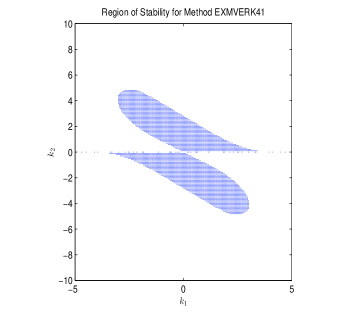
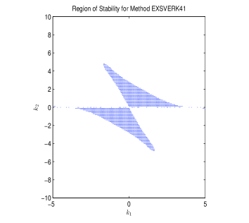
Figure 1: (a): Stability region for fourth-order explicit MVERK (EXMVERK41) method (10) with two stages. (b): Stability region for fourth-order explicit MVERK (EXMVERK41) method (10) with two stages.

The stability regions of fourth-order explicit ERK method (10) and (20) are respectively depicted in Fig. 1 (a) and (b). In recent work [33], we only verify the convergence of first-order explicit ERK methods in detail, but the convergence of higher-order explicit ERK methods is not discussed. Hence we will analyze the convergence of the higher-order explicit ERK methods in this paper. The convergence of the fourth-order explicit SVERK methods will be displayed in this section, and the convergence of the fourth-order explicit MVERK methods can be analyzed in the same way which will be skipped for brevity.

Assumption 4.1

Suppose that (1) has a sufficiently smooth solution $y:[t_{0},t_{end}]\rightarrow X.$ Let f be locally Lipschitz-continuous in a strip along the exact solution $y$, i.e., there exists a real number $L>0$ for all $t\in[t_{0},t_{end}]$, such that $\|f(y)-f(\hat{y})\|\leq L\|y-\hat{y}\|.$

The following theorem shows the convergence of the fourth-order explicit SVERK methods.

Theorem 4.2

Under Assumption 4.1, if the four-stage explicit SVERK method with $\bar{w}_{4}(z)$ satisfies the order conditions (8), then the upper bound of global error has the following form

$$\|y_{n}-y(t_{n})\|\leq Ch^{4},$$

where $1\leq n\leq\frac{t_{end}-t_{0}}{h}$. The constant $C$ is independent of $n$ and $h$, but depends on $t_{end},\ \|M\|,\ f^{(p)}(t_{n})$ for $p=0,\ldots,5.$

Proof.   We rewrite the four-stage explicit SVERK method (3) as

$$\left\{\begin{array}[]{l}\displaystyle k_{n,1}=f(y_{n}),\cr\vskip 11.38109pt\cr\displaystyle k_{n,2}=f(e^{-\bar{c}_{2}hM}y_{n}+h\bar{a}_{21}k_{n,1}),\cr\vskip 11.38109pt\cr\displaystyle k_{n,3}=f\big{(}e^{-\bar{c}_{3}hM}y_{n}+h(\bar{a}_{31}k_{n,1}+\bar{a}_{32}k_{n,2})\big{)},\cr\vskip 11.38109pt\cr\displaystyle k_{n,4}=f\big{(}e^{-\bar{c}_{4}hM}y_{n}+h(\bar{a}_{41}k_{n,1}+\bar{a}_{42}k_{n,2}+\bar{a}_{43}k_{n,3})\big{)},\cr\vskip 11.38109pt\cr\displaystyle y_{n+1}=e^{-hM}y_{n}+h\big{(}\bar{b}_{1}k_{n,1}+\bar{b}_{2}k_{n,2}+\bar{b}_{3}k_{n,3}+\bar{b}_{4}k_{n,4}\big{)}+\bar{w}_{4}(z),\end{array}\right.$$ (26)

and expand $y(t_{n}+h)$ into a Taylor series

$$y(t_{n}+h)=y(t_{n})+hy^{\prime}(t_{n})+\frac{h^{2}}{2!}y^{\prime\prime}(t_{n})+\frac{h^{3}}{3!}y^{\prime\prime\prime}(t_{n})+\frac{h^{4}}{4!}y^{(4)}(t_{n})+Ch^{5}.$$ (27)

Inserting the exact solution into the numerical scheme gives

$$y(t_{n}+h)=e^{-hM}y(t_{n})+h\big{(}\bar{b}_{1}\bar{k}_{n,1}+\bar{b}_{2}\bar{k}_{n,2}+\bar{b}_{3}\bar{k}_{n,3}+\bar{b}_{4}\bar{k}_{n,4}\big{)}+\hat{w}_{4}(z)+\delta_{n+1},$$ (28)

where

$$\delta_{n+1} =y(t_{n})+hy^{\prime}(t_{n})+\frac{h^{2}}{2!}y^{\prime\prime}(t_{n})+\frac{h^{3}}{3!}y^{\prime\prime\prime}(t_{n})+\frac{h^{4}}{4!}y^{(4)}(t_{n})+Ch^{5}-e^{-hM}y(t_{n})$$ (29)

$$\quad-h\big{(}\bar{b}_{1}\bar{k}_{n,1}+\bar{b}_{2}\bar{k}_{n,2}+\bar{b}_{3}\bar{k}_{n,3}+\bar{b}_{4}\bar{k}_{n,4}\big{)}-\hat{w}_{4}(z),$$

$\bar{k}_{n,1},\ \bar{k}_{n,2},\ \bar{k}_{n,3},\ \bar{k}_{n,4}$ and $\hat{w}_{4}(z)$ correspond to $k_{n,,1},\ k_{n,2},\ k_{n,3},\ k_{n,4}$ and $\bar{w}_{4}(z)$, which are satisfying $y(t_{n})=y_{n}$, respectively.

If we denote $E_{n-1,i}=k_{n-1,i}-\bar{k}_{n-1,i}$ and $e_{n}=y_{n}-y(t_{n})$ , then

$$E_{n-1,i} =f(e^{-\bar{c}_{i}hM}y_{n-1}+h\sum\limits_{j=1}^{i-1}\bar{a}_{ij}k_{n-1,j})-f(e^{-\bar{c}_{i}hM}y(t_{n-1})+h\sum\limits_{j=1}^{i-1}\bar{a}_{ij}\bar{k}_{n-1,j}),$$ (30)

$$e_{n} =e^{-hM}e_{n-1}+h\sum\limits_{i=1}^{4}\bar{b}_{i}\big{(}k_{n-1,i}-\bar{k}_{n-1,i}\big{)}+\bar{w}_{4}(z)-\hat{w}_{4}(z)-\delta_{n}.$$

It follows from the first formula of (30) that

$$E_{l,1} =f(y_{l})-f(y(t_{l})),$$ (31)

$$E_{l,2} =f(e^{-\bar{c}_{2}hM}y_{l}+h\bar{a}_{21}k_{l,1})-f(e^{-\bar{c}_{2}hM}y(t_{l})+h\bar{a}_{21}\bar{k}_{l,1}),$$

$$E_{l,3} =f(e^{-\bar{c}_{3}hM}y_{l}+h\bar{a}_{31}k_{l,1}+h\bar{a}_{32}k_{l,2})-f(e^{-\bar{c}_{3}hM}y(t_{l})+h\bar{a}_{31}\bar{k}_{l,1}+h\bar{a}_{32}\bar{k}_{l,2}),$$

$$E_{l,4} =f(e^{-\bar{c}_{4}hM}y_{l}+h\bar{a}_{41}k_{l,1}+h\bar{a}_{42}k_{l,2}+h\bar{a}_{43}k_{l,3})-f(e^{-\bar{c}_{4}hM}y(t_{l})+h\bar{a}_{41}\bar{k}_{l,1}+h\bar{a}_{42}\bar{k}_{l,2}+h\bar{a}_{43}\bar{k}_{l,3}).$$

The formula (31) holds for $l=0,\ldots,n-1$. In what follows, we consider the Taylor series for $\bar{k}_{l,1},\ \bar{k}_{l,2},\ \bar{k}_{l,3},\ \bar{k}_{l,4}$, and then $\delta_{l+1}$ satisfies

$$\delta_{l+1} =y(t_{l})+hy^{\prime}(t_{l})+\frac{h^{2}}{2!}y^{\prime\prime}(t_{l})+\frac{h^{3}}{3!}y^{\prime\prime\prime}(t_{l})+\frac{h^{4}}{4!}y^{(4)}(t_{l})+Ch^{5}-e^{-hM}y(t_{l})-h\big{(}\bar{b}_{1}\bar{k}_{l,1}+\bar{b}_{2}\bar{k}_{l,2}+\bar{b}_{3}\bar{k}_{l,3}+\bar{b}_{4}\bar{k}_{l,4}\big{)}$$

$$\quad-\hat{w}_{4}(z)$$

$$=y(t_{l})+hg(t_{l})+\frac{h^{2}}{2!}(-M+f^{\prime}_{y}(y_{l}))g(t_{l})+\frac{h^{3}}{3!}\Big{(}M^{2}g(t_{l})+(-M+f^{\prime}_{y}(y(t_{l})))f^{\prime}_{y}(y(t_{l}))g(t_{l})-f^{\prime}_{y}(y(t_{l}))Mg(t_{l})$$

$$+f^{\prime\prime}_{yy}(y(t_{l}))(g(t_{l}),g(t_{l}))\Big{)}+\frac{h^{4}}{4!}\Big{(}-M^{3}g(t_{l})+M^{2}f^{\prime}_{y}(y(t_{l}))g(t_{l})-Mf^{\prime}_{y}(y(t_{l}))(-M+f^{\prime}_{y}(y(t_{l})))g(t_{l})$$

$$-Mf^{\prime\prime}_{yy}(y(t_{l}))(g(t_{l}),g(t_{l}))+f^{\prime\prime\prime}_{yyy}(y(t_{l}))(g(t_{l}),g(t_{l}),g(t_{l}))+3f^{\prime\prime}_{yy}(y(t_{l}))\big{(}(-M+f^{\prime}_{y}(y(t_{l})))g(t_{l}),g(t_{l})\big{)}$$

$$+f^{\prime}_{y}(y(t_{l}))(-M+f^{\prime}_{y}(y(t_{l})))(-M+f^{\prime}_{y}(y(t_{l})))g(t_{l})+f^{\prime}_{y}(y(t_{l}))f^{\prime\prime}_{yy}(y(t_{l}))(g(t_{l}),g(t_{l}))\Big{)}+Ch^{5}$$

$$-\Bigg{\{}y(t_{l})-hMy(t_{l})+h(\bar{b}_{1}+\bar{b}_{2}+\bar{b}_{3}+\bar{b}_{4})f(y(t_{l}))-\frac{h^{2}Mg(y(t_{l}))}{2!}+h^{2}(\bar{b}_{2}\bar{c}_{2}+\bar{b}_{3}\bar{c}_{3}+\bar{b}_{4}\bar{c}_{4})f^{\prime}_{y}(y(t_{l}))g(t_{l})$$

$$-\frac{h^{3}}{3!}f^{\prime}_{y}(y(t_{l}))Mf(y(t_{l}))+\frac{h^{3}}{3!}M(M-f^{\prime}_{y}(y(t_{l}))g(t_{l})+\frac{h^{3}}{2!}(\bar{b}_{2}\bar{c}_{2}^{2}+\bar{b}_{3}\bar{c}_{3}^{2}+\bar{b}_{4}\bar{c}_{4}^{2})f^{\prime\prime}_{yy}(y(t_{l}))(g(t_{l}),g(t_{l}))$$

$$+h^{3}(\bar{b}_{3}\bar{a}_{32}\bar{c}_{2}+\bar{b}_{4}(\bar{a}_{42}\bar{c}_{2}+\bar{a}_{43}\bar{c}_{3}))f^{\prime}_{y}(y(t_{l}))(M^{2}y(t_{l})+f^{\prime}_{y}(y(t_{l}))g(t_{l}))+\frac{h^{4}}{4!}\Big{(}-M^{3}g(t_{l})+M^{2}f^{\prime}_{y}(y(t_{l}))g(t_{l})$$

$$-Mf^{\prime\prime}_{yy}(y(t_{l}))(g(t_{l}),g(t_{l}))-Mf^{\prime}_{y}(y(t_{l}))(-M+f^{\prime}_{y}(y(t_{l})))g(t_{l})-f^{\prime}_{y}(y_{l})Mf^{\prime}_{y}(y(t_{l}))g(t_{l})-f^{\prime}_{y}(y(t_{l}))f^{\prime}_{y}(y(t_{l}))$$

$$\cdot Mf(y(t_{l}))+3f^{\prime\prime}_{yy}(y(t_{l}))(-Mf(y(t_{l})),g(t_{l}))\Big{)}+h^{4}\bar{b}_{4}\bar{a}_{43}\bar{a}_{32}\bar{a}_{21}f^{\prime}_{y}(y(t_{l}))\big{(}(M^{2}+f^{\prime}_{y}(y(t_{l}))^{2})g(t_{l})+f^{\prime}_{y}(y(t_{l}))^{2}$$

$$\cdot M^{2}y(t_{l})\big{)}+\frac{h^{4}}{3!}(\bar{b}_{2}\bar{c}_{2}^{3}+\bar{b}_{3}\bar{c}_{3}^{3}+\bar{b}_{4}\bar{c}_{4}^{3})f^{\prime\prime\prime}_{yyy}(y(t_{l}))\big{(}g(t_{l}),g(t_{l}),g(t_{l})\big{)}+\frac{h^{4}}{2!}(\bar{b}_{3}\bar{a}_{32}\bar{c}_{2}^{2}+\bar{b}_{4}\bar{a}_{42}\bar{c}_{2}^{2}+\bar{b}_{4}\bar{a}_{43}\bar{c}_{3}^{2})f^{\prime}_{y}(y(t_{l}))$$

$$\cdot f^{\prime\prime}_{yy}(y(t_{l}))\big{(}g(t_{l}),g(t_{l})\big{)}+h^{4}(\bar{b}_{3}\bar{c}_{3}\bar{a}_{32}\bar{a}_{21}+\bar{b}_{4}\bar{c}_{4}\bar{a}_{42}\bar{c}_{2}+\bar{b}_{4}\bar{c}_{4}\bar{a}_{43}\bar{c}_{3})f^{\prime\prime}_{yy}(y(t_{l}))\big{(}M^{2}y(t_{l})+f^{\prime}_{y}(y(t_{l}))g(t_{l}),g(t_{l})\big{)}\Bigg{\}},$$

where $g(t_{l})=-My(t_{l})+f(y(t_{l}))$. Since the coefficients of the explicit SVERK method satisfies the order conditions (8), one has

$$\delta_{l+1}=Ch^{5}.$$ (32)

Taking the norm $\|\cdot\|$ for the second formula of (30) and (31) yields

$$\|E_{l,1}\| \leq L\|e_{l}\|,$$ (33)

$$\|E_{l,2}\| \leq L\|e^{-\bar{c}_{2}hM}e_{l}+h\bar{a}_{21}(k_{l,1}-\bar{k}_{l,1})\|\leq L(1+h|\bar{a}_{21}|L)\|e_{l}\|,$$

$$\|E_{l,3}\| \leq L\|e^{-\bar{c}_{3}hM}e_{l}+h\bar{a}_{31}(k_{l,1}-\bar{k}_{l,1})+h\bar{a}_{32}(k_{l,2}-\bar{k}_{l,2})\|$$

$$\leq L\|e^{-\bar{c}_{3}hM}e_{l}\|+Lh|\bar{a}_{31}|\cdot\|E_{l,1}\|+Lh|\bar{a}_{32}|\cdot\|E_{l,2}\|$$

$$\leq L\big{(}1+h|\bar{a}_{31}|L+h|\bar{a}_{32}|L(1+h|\bar{a}_{21}|L)\big{)}\|e_{l}\|=L(1+h|\bar{a}_{31}|L+h|\bar{a}_{32}|L+h^{2}|\bar{a}_{32}|\cdot|\bar{a}_{21}|L^{2})\|e_{l}\|,$$

$$\|E_{l,4}\| \leq L\|e^{-\bar{c}_{4}hM}e_{l}+h\bar{a}_{41}(k_{l,1}-\bar{k}_{l,1})+h\bar{a}_{42}(k_{l,2}-\bar{k}_{l,2})+h\bar{a}_{43}(k_{l,3}-\bar{k}_{l,3})\|$$

$$\leq L\|e^{-\bar{c}_{4}hM}e_{l}\|+Lh|\bar{a}_{41}|\cdot\|E_{l,1}\|+Lh|\bar{a}_{42}|\cdot\|E_{l,2}\|+Lh|\bar{a}_{43}|\cdot\|E_{l,3}\|$$

$$\leq L(1+h|\bar{a}_{41}|L+h|\bar{a}_{42}|L(1+h|\bar{a}_{21}|L)+h|\bar{a}_{43}|L(1+h|\bar{a}_{31}|L+h|\bar{a}_{32}|L+h^{2}|\bar{a}_{32}|\cdot|a_{21}|L^{2}))\|e_{l}\|$$

$$=L(1+h(|\bar{a}_{41}|+|\bar{a}_{42}|+|\bar{a}_{43}|)L+h^{2}(|\bar{a}_{42}|\cdot|\bar{a}_{21}|+|\bar{a}_{43}|\cdot|\bar{a}_{31}|+|\bar{a}_{43}|\cdot|\bar{a}_{32}|)L^{2}+h^{3}|\bar{a}_{43}|\cdot|\bar{a}_{32}|\cdot|\bar{a}_{21}|L^{3})\|e_{l}\|,$$

and

$$\|e_{n}\|\leq\|e_{n-1}\|+h\sum\limits_{i=1}^{4}|\bar{b}_{i}|\cdot\|E_{n-1,i}\|+\|\bar{w}_{4}(z)-\hat{w}_{4}(z)\|+Ch^{5},$$

where $C$ depends on $T,\ \|M\|$, $f^{(p)}(t_{n})$, $p=0,\ldots,5$, but is independent of $n$ and $h$. According to the expressions of $\bar{w}_{4}(z)$ and $\hat{w}_{4}(z)$, one gets

$$\|\bar{w}_{4}(z)-\hat{w}_{4}(z)\|\leq Ch^{2}L\|e_{n}\|+Ch^{3}L\|e_{n}\|+Ch^{4}L\|e_{n}\|.$$ (34)

It follows from (33) that

$$h\sum\limits_{i=1}^{4}|\bar{b}_{i}|\cdot\|E_{l,i}\| \leq ChL\|e_{l}\|+Ch^{2}L^{2}\|e_{l}\|+Ch^{3}L^{3}\|e_{l}\|+Ch^{4}L^{4}\|e_{l}\|,\ l=0,\ldots,n-1.$$ (35)

We then obtain

$$\|e_{n}\| \leq\|e_{n-1}\|+h\sum\limits_{i=1}^{4}|\bar{b}_{i}|\cdot\|E_{n-1,i}\|+Ch^{2}L\|e_{n-1}\|+Ch^{3}L\|e_{n-1}\|+Ch^{4}L\|e_{n-1}\|+Ch^{5}$$ (36)

$$\leq\|e_{1}\|+\sum\limits_{l=1}^{n-1}\big{(}Ch\sum\limits_{i=1}^{4}\|E_{l,i}\|+Ch^{2}L\|e_{l}\|+Ch^{3}L\|e_{l}\|+Ch^{4}L\|e_{l}\|\big{)}+(n-1)Ch^{5}$$

$$\leq\sum\limits_{l=1}^{n-1}Ch\big{(}\sum\limits_{i=1}^{4}\|E_{l,i}\|+hL\|e_{l}\|+h^{2}L\|e_{l}\|+h^{3}L\|e_{l}\|\big{)}+Ch^{4}.$$

Inserting (35) into (36) leads to

$$\|e_{n}\|\leq\sum\limits_{l=1}^{n-1}ChL\big{(}\|e_{l}\|+hL\|e_{l}\|+h^{2}L^{2}\|e_{l}\|+h^{3}L^{3}\|e_{l}\|\big{)}+Ch^{4}.$$ (37)

The application of the discrete Gronwall lemma to (37) gives

$$\|e_{n}\|\leq Ch^{4},$$ (38)

which completes the proof. $\hfill\square$

5 Numerical Experiments

In this section, we conduct some numerical experiments to show that the fourth-order explicit MVERK and SVERK methods have comparable accuracy and efficiency by comparing with the standard fourth-order explicit ERK integrators. Throughout the numerical experiments, the entire functions $\varphi_{i}(-k_{n}M)$ of exponential integrators be evaluated by the Krylov subspace method (see, e.g., [4, 17]), which has the fast convergence. We select the following fourth-order ERK methods for comparison:

• ERK41: the fourth-order (stiff) explicit exponential RK method (12) with five stages in [19];

• ERK42: the fourth-order (stiff) explicit exponential RK method (13) with four stages in [22];

• MVERK41: the fourth-order (non-stiff) explicit MVERK method (10) with four stages presented in this paper;

• MVERK42: the fourth-order (non-stiff) explicit MVERK method (15) with four stages presented in this paper;

• SVERK41: the fourth-order (non-stiff) explicit SVERK method (20) with four stages presented in this paper;

• SVERK42: the fourth-order (non-stiff) explicit SVERK method (22) with four stages presented in this paper.

Problem 1.  We first consider the following averaged system in wind-induced oscillation ([26])

$$\left(\begin{array}[]{c}x_{1}\\ x_{2}\\ \end{array}\right)^{\prime}=\left(\begin{array}[]{cc}-\zeta&-\lambda\\ \lambda&-\zeta\\ \end{array}\right)\left(\begin{array}[]{c}x_{1}\\ x_{2}\\ \end{array}\right)+\left(\begin{array}[]{c}x_{1}x_{2}\\ \frac{1}{2}(x_{1}^{2}-x_{2}^{2})\end{array}\right),$$

where $\zeta\geq 0$ is a damping factor and $\lambda$ is a detuning parameter (see, e.g., [14]). Set

$$\zeta=r\cos(\theta),\ \lambda=r\sin(\theta),\ r\geq 0,\ 0\leq\theta\leq\pi/2.$$

This system can be written as

$$\left(\begin{array}[]{c}x_{1}\\ x_{2}\\ \end{array}\right)^{\prime}=\left(\begin{array}[]{cc}-\cos(\theta)&-\sin(\theta)\\ \sin(\theta)&-\cos(\theta)\\ \end{array}\right)\left(\begin{array}[]{c}rx_{1}-\frac{1}{2}\sin(\theta)(x_{2}^{2}-x_{1}^{2})-\cos(\theta)x_{1}x_{2}\\ rx_{2}-\sin(\theta)x_{1}x_{2}+\frac{1}{2}\cos(\theta)(x_{2}^{2}-x_{1}^{2})\end{array}\right).$$

We integrate the conservative system over the interval $[0,100]$ with parameters $\theta=\pi/2,\ r=20$ and stepsizes $h=1/2^{k}$ for $k=4,\ldots,8$. Fig. 2 displays the global errors $GE$ against the stepsizes and the CPU time. From Fig. 2, we observe that our methods have the same accuracy with standard fourth-order explicit exponential integrators, and present the higher efficiency than exponential integrators is supported by their less CPU times (seconds).

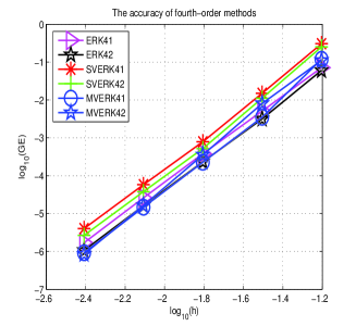
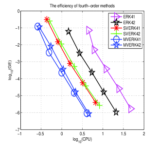
Figure 2: Results for accuracy of Problem 5. a: The $\log$-$\log$ plots of global errors (GE) against $h$. b: The $\log$-$\log$ plots of global errors against the CPU time.

Problem 2.  The Hénon-Heiles Model was used to describe the stellar motion (see, e.g., [15, 16]), which has the following identical form

$$\left(\begin{array}[]{c}x_{1}\\ x_{2}\\ y_{1}\\ y_{2}\\ \end{array}\right)^{\prime}+\left(\begin{array}[]{cccc}0&0&-1&0\\ 0&0&0&-1\\ 1&0&0&0\\ 0&1&0&0\\ \end{array}\right)\left(\begin{array}[]{c}x_{1}\\ x_{2}\\ y_{1}\\ y_{2}\\ \end{array}\right)=\left(\begin{array}[]{c}0\\ 0\\ -2x_{1}x_{2}\\ -x_{1}^{2}+x_{2}^{2}\\ \end{array}\right).$$

We select the initial values as

$$\big{(}x_{1}(0),x_{2}(0),y_{1}(0),y_{2}(0)\big{)}^{\intercal}=(\sqrt{\frac{11}{96}},0,0,\frac{1}{4})^{\intercal}.$$

Fig. 3 presents that this problem is solved on the interval $[0,10]$ with stepsizes $h=1/2^{k},\ k=3,\ldots,7$ for ERK41, ERK42, SVERK41, SVERK42, MVERK41, and MVERK42. It can be observed that our methods have the comparable accuracy with ERK41 and ERK42, and present the higher efficiency than ERK41 and ERK42.

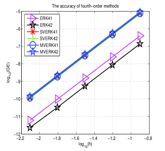
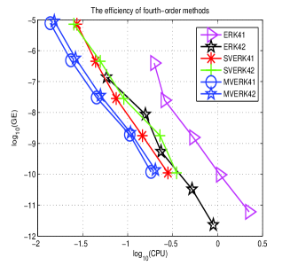
Figure 3: Results for Problem 2. a: The $\log$-$\log$ plots of global errors (GE) against $h$. b: The $\log$-$\log$ plots of global errors against the CPU time.

Problem 3.  We consider the Allen-Cahn equation [2, 12]

$$\left\{\begin{aligned} &\frac{\partial u}{\partial t}=\epsilon\frac{\partial^{2}u}{\partial x^{2}}+u-u^{3},\quad-1<x<1,\ t>0,\\ &u(x,0)=0.53x+0.47\sin(-1.5\pi x),\quad-1\leq x\leq 1.\end{aligned}\right.$$

Allen and Cahn firstly introduced the equation to describe the motion of anti-phase boundaries in crystalline solids [2]. After approximating the spatial derivatives with 32-point Chebyshev spectral method, we obtain the following stiff system of first-order ordinary differential equations

$$\frac{dU}{dt}+MU=F(t,U),\quad t\in[0,t_{\rm end}],$$

where $U(t)=(u_{1}(t),\cdots,u_{N}(t))^{\intercal},$ $u_{i}(t)\approx u(x_{i},t),\ x_{i}=-1+i\Delta x$, for $i=1,{\ldots},N$ and $\Delta x=2/N$. Here, the matrix $M$ is full and the nonlinear term is $F(t,U)=u-u^{3}=(u_{1}-u_{1}^{3},\cdots,u_{N}-u_{N}^{3})^{\intercal}.$ We choose the parameters $\epsilon=0.01,\ N=32$ and integrate the obtained stiff system over the interval $[0,1]$. The numerical results are presented in Fig. 4 with the stepsizes $h=1/2^{k}$ for $k=8,\ldots,12$.

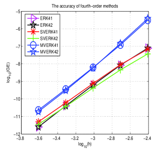
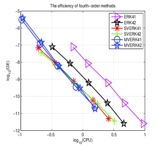
Figure 4: Results for accuracy of Problem 3. a: The $\log$-$\log$ plots of global errors (GE) against $h$. b: The $\log$-$\log$ plots of global errors against the CPU time.

Problem 4.  Consider the sine-Gorden equation with periodic boundary conditions [11, 13]

$$\left\{\begin{array}[]{l}\dfrac{\partial^{2}u}{\partial t^{2}}=\dfrac{\partial^{2}u}{\partial x^{2}}-\sin(u),\quad-1<x<1,t>0,\cr\vskip 2.84526pt\cr u(-1,t)=u(1,t).\cr\vskip 2.84526pt\cr\end{array}\right.$$

Discretising the spatial derivative $\partial_{xx}$ by the second-order symmetric differences yields

$$\frac{d}{dt}\left(\begin{array}[c]{c}U^{\prime}\\ U\\ \end{array}\right)+\left(\begin{array}[c]{cc}{\bf 0}&M\\ -I&{\bf 0}\\ \end{array}\right)\left(\begin{array}[c]{c}U^{\prime}\\ U\\ \end{array}\right)=\left(\begin{array}[c]{c}-\sin(U)\\ {\bf 0}\\ \end{array}\right),\quad t\in[0,t_{\rm end}].$$

In here, $U(t)=(u_{1}(t),\cdots,u_{N}(t))^{T}$ with $u_{i}(t)\approx u(x_{i},t)$ for $i=1,\ldots,N$, with $\Delta x=2/N$ and $x_{i}=-1+i\Delta x$, $F(t,U)=-\sin(u)=-(\sin(u_{1}),\cdots,\sin(u_{N}))^{T}$, and

$$M=\dfrac{1}{\Delta x^{2}}\left(\begin{array}[c]{ccccc}2&-1&&&-1\\ -1&2&-1&&\\ &\ddots&\ddots&\ddots&\\ &&-1&2&-1\\ -1&&&-1&2\\ \end{array}\right).$$

In this test, we choose the initial value conditions

$$U(0)=(\pi)^{N}_{i=1},\ U^{\prime}(0)=\sqrt{N}\left(0.01+\sin(\dfrac{2\pi i}{N})\right)_{i=1}^{N}$$

with $N=32$, and solve the problem on the interval $[0,1]$ with stepsizes $h=1/2^{k},\ k=4,\ldots,8$. The global errors GE against the stepsizes and the CPU time (seconds) for ERK41, ERK42, SVERK41, SVERK42, MVERK41 and MVERK42 are respectively presented in Fig. 5 (a) and (b).

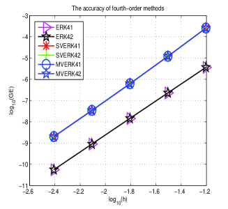
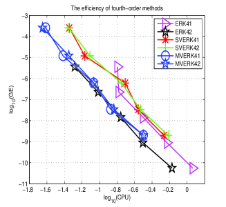
Figure 5: Results for Problem 4. a: The $\log$-$\log$ plots of global errors (GE) against $h$. b: The $\log$-$\log$ plots of global errors against the CPU time.

Problem 5.  We consider the nonlinear Schrödinger equation (see [9])

$$i\psi_{t}+\psi_{xx}+2|\psi|^{2}\psi=0,\quad\psi(x,0)=0.5+0.025\cos(\mu x),$$

with the periodic boundary condition $\psi(0,t)=\psi(L,t).$ Letting $L=4\sqrt{2}\pi$ and $\mu=2\pi/L$ and $\psi=p+\textmd{i}q,$ we transform this equation into a pair of real-valued equations

$$p_{t}+q_{xx}+2(p^{2}+q^{2})q=0,$$

$$q_{t}-p_{xx}-2(p^{2}+q^{2})p=0.$$

Using the discretization on spatial variable with the pseudospectral method leads to

$$\left(\begin{array}[]{c}\textbf{p}\\ \textbf{q}\\ \end{array}\right)^{\prime}=\begin{aligned} \left(\begin{array}[]{cc}0&-D_{2}\\ D_{2}&0\\ \end{array}\right)\left(\begin{array}[]{c}\textbf{p}\\ \textbf{q}\\ \end{array}\right)+\left(\begin{array}[]{c}-2(\textbf{p}^{2}+\textbf{q}^{2})\cdot\textbf{q}\\ 2(\textbf{p}^{2}+\textbf{q}^{2})\cdot\textbf{p}\\ \end{array}\right)\end{aligned}$$ (39)

where $\textbf{p}=(p_{0},p_{1},\ldots,p_{N-1})^{\intercal},\ \textbf{q}=(q_{0},q_{1},\ldots,q_{N-1})^{\intercal}$ and $D_{2}=(D_{2})_{0\leq j,k\leq N-1}$ is the pseudospectral differential matrix defined by:

$$(D_{2})_{jk}=\left\{\begin{aligned} &\frac{1}{2}\mu^{2}(-1)^{j+k+1}\frac{1}{\sin^{2}(\mu(x_{j}-x_{k})/2)},\quad j\neq k,\\ &-\mu^{2}\frac{2(N/2)^{2}+1}{6},\quad\quad\quad\quad\quad\quad\ \ \ \ \ j=k.\end{aligned}\right.$$

In this test, we choose $N=48$ and solve this problem on $[0,1]$. The global errors $GE$ against the stepsizes and the CPU time are stated in Fig. 6 with the stepsizes $h=1/2^{k}$ for $k=4,\ldots,8$.

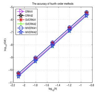
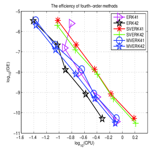
Figure 6: Results for accuracy of Problem 5. a: The $\log$-$\log$ plots of global errors (GE) against $h$. b: The $\log$-$\log$ plots of global errors against the CPU time.

6 Conclusion

ERK integrators for solving stiff problems or highly oscillatory systems have distinguished advantages which have been received lots of attention in recent years. However, the computational cost of standard ERK methods heavily depends on evaluations of matrix exponentials. In order to reduce the computational cost, we have designed two classes of explicit ERK methods up to order three. As a sequel to our previous work, we formulate two new families of fourth-order explicit ERK methods for solving stiff or highly oscillatory systems in this paper. We derive the order conditions of these fourth-order explicit ERK methods, which are exactly identical to those of the classical fourth-order explicit RK methods. These fourth-order MVERK and SVERK methods have the favorable property that they can exactly integrate the linear systems $y^{\prime}(t)+My(t)=0$ than RK methods. Moreover, the coefficients of these methods are real constants so that they can effectively reduce the computational cost compared with standard ERK methods. Furthermore, the convergence of these methods was analyzed in detail.

Several numerical examples are carried out to demonstrate the comparable accuracy and lower computational cost of these fourth-order explicit ERK methods in comparison with the standard fourth-order explicit exponential integrators in the literature. It is noted that our study is related to the classical order conditions, order reduction phenomenon of our methods can be observed when applied to some multi-frequency and high-dimension problems.

As a preliminary study of MVERK and SVERK methods, our convergence analysis of this paper depends on the Taylor series of the exact solution, so that the constant $C$ depends on $\|M\|$. This is not favorable. Therefore, an improved convergence analysis is still needed and we will pay attention to this aspect in our next work.

References

References

[1]
C. Abhulimen,
Exponentially fitted third derivative three-step methods for numerical
integration of stiff initial value problems,
Appl. Math. Comput. 243 (2014) 446-453.
[2]
S. M. Allen, J. W. Cahn,
A microscopic theory for antiphase boundary motion and
its application to antiphase domain coarsening,
Acta Metallurgica. 27 (1979) 1085-1095.
[3]
H. Berland, B. Owren, B. Skaflestad,
B-series and order conditions for exponential integrators,
SIAM J. Numer. Anal. 43 (2005) 1715-1727.
[4]
H. Berland, B. Skaflestad, W. Wright,
EXPINT–A MATLAB package for exponential integrators,
ACM Trans. Math. Softw. 33(2007) 4.
[5]
J. C. Butcher,
Numerical Methods for Ordinary Diffrential Equations,
Second edition, John Wiley & Sons, Ltd, 2008.
[6]
T. Buvoli, M. L. Minion,
On the stability of exponential integrators for non-diffusive
equations,
J. Comput. Appl. Math. 409 (2022) 114126.
[7]
E. Celledoni, D. Cohen, B. Owren,
Symmetric exponential integrators with an application
to the cubic Schröinger equation,
Found. Comput. Math. 8 (2008) 303-317.
[8]J. R. Cash, Second derivative
extended backward differentiation formulas for the numerical
integration of stiff systems, SIAM J. Numer. Anal. 18 (1981) 21-36.
[9]
J. Chen, M. Qin,
Multisymplectic Fourier pseudospectral method for the nonlinear
Schrödinger equation,
Electron. Trans. Numer. Anal. 12 (2001) 193-204.
[10]
W. H. Enright,
Second derivative multistep methods for stiff ordinary diffential equations,
SIAM J. Numer. Anal. 11 (1974) 321-331.
[11]
Y. Fang, X. Hu, J. Li,
Explicit pseudo two-step exponential Runge-Kutta methods for the numerical
integration of first-order differential equations,
Numer. Algor. 86 (2021) 1143-1163.
[12]
X. Feng, H. Song, T. Tang, J. Yang,
Nonlinear stability of the implicit-explicit methods for the Allen-Cahn equation,
Inverse Problems and Imaging. 7 (2013) 679-695.
[13]
J. M. Franco,
New methods for oscillatory systems based on ARKN methods,
Appl. Numer. Math.
56 (2006) 1040-1053.
[14]
J. Guckenheimer, P. Holmes, Nonlinear Oscillations. Dynamical Systems, and Bifurcations of Vector Fields, Springer-Verlag, New York, 1983.
[15]
E. Hairer, C. Lubich, G. Wanner, Geometric Numerical Integration: Structure-Preserving Algorithms
for Ordinary Differential Equations, 2nd edn. Springer, Berlin (2006).
[16]
M. Hénon, C. Heiles, The applicability of the third integral of motion: some numerical
experiments, Astron. J. 69 (1964) 73-79.
[17]
M. Hochbruck, C. Lubich, On Krylov subspace approximations to
the matrix exponential operator, SIAM J. Numer. Anal. 34 (1997) 1911-1925.
[18]
M. Hochbruck, C. Lubich, H. Selhofer,
Exponential integrators for large systems of differential equations,
SIAM J. Sci. Comput. 19 (1998) 1552-1574.
[19]
M. Hochbruck, A. Ostermann,
Explicit exponential Runge-Kutta methods for semilinear
parabolic problems,
SIAM J. Numer. Anal. 43 (2005) 1069-1090.
[20]
M. Hochbruck, A. Ostermann,
Exponential Runge-Kutta methods for parabolic problems,
Appl. Numer. Math. 53 (2005) 323-339.
[21]
M. Hochbruck, A. Ostermann,
Exponential integrators,
Acta Numer. 19 (2010) 209-286.
[22]
S. Krogstad,
Generalized integrating factor methods for stiff PDEs,
J. Comput. Phys. 203
(2005) 72-88.
[23]
J. D. Lawson,
Generalized Runge-Kutta processes for stable
systems with large Lipschitz constants,
SIAM J. Numer. Anal. 4 (1967) 372-380.
[24]
J. D. Lambert, S. T. Sigurdsson,
Multistep methods with variable matrix coefficients,
SIAM J. Numer. Anal. 9 (1972) 715-733.
[25]
Y. Li, X. Wu,
Exponential integrators preserving first integrals
or Lyapunov functions for conservative or dissipative systems,
SIAM J. Sci. Comput. 38 (2016) A1876-A1895.
[26]
R. I. Mclachlan, G. R. W. Quispel, N. Robidoux,
A unified approach to Hamiltonian systems, Poisson systems,
gradient systems, and systems with Lyapunov functions or first integrals,
Phys. Rev. Lett. 81 (1998) 2399-2411.
[27]
L. Mei, L. Huang, X. Wu,
Energy-preserving continuous-stage exponential Runge-Kutta
integrators for efficiently solving Hamiltonian systems,
SIAM J. Sci. Comput. 44 (2022) A1092-A1115.
[28]
S. Norsett, An A-stable modification of the Adams-Bashforth methods,
in Conference on the Numerical Solution of Differential Equations,
J. Morris, ed.,
Lecture Notes in Math.
Springer, Berlin, 109 (1969) 214-219.
[29]
D. Pope,
An exponential method of numerical integration of ordinary differential equations,
Comm. ACM. 6 (1963) 491-493.
[30]
R. Qi, C. Zhang, Y. Zhang,
Dissipativity of multistep Runge-Kutta methods for nonlinear
volterra delay-integro-differential equations,
Acta Math. Appl. Sin. Engl. Ser. 28 (2012) 225-236.
[31]
B. Wang, X. Wu,
Exponential collocation methods for conservative or dissipative systems,
J. Comput. Appl. Math. 360 (2019) 99-116.
[32]
B. Wang, X. Wu,
Geometric Integrators for Differential Equations
with Highly Oscillatory Solutions, Springer Nature Singapore Pte Ltd. 2021.
[33]
B. Wang, X. Hu, X. Wu,
Two new classes of exponential Runge-Kutta integrators
for efficiently solving stiff systems or highly oscillatory problems, arXiv: 2210.00685. 2022.
[34]
W. Wang, C. Zhang,
Dissipativity of variable-stepsize Runge-Kutta methods for nonlinear functional differential equations with application to Nicholsons blowflies models,
Commun. Nonlinear. Sci. Numer. Simul. 97 (2021) 105723.
[35]
X. Wu, B. Wang,
Recent Developments in Structure-Preserving Algorithms for Oscillatory Differential Equations, Springer-Verlag, Singapore, 2018.
[36]
C. Zhang, T. Qin,
The mixed Runge-Kutta methods for a class of nonlinear functional-integro-differential equations,
Appl. Math. Comput. 237 (2014) 396-404.