Deep-Circuit QAOA
Abstract
Despite its popularity, several empirical and theoretical studies suggest that the quantum approximate optimization algorithm (QAOA) has persistent issues in providing a substantial practical advantage. So far, those findings mostly account for a regime of few qubits and shallow circuits. We find clear evidence for a ‘no free lunch’-behavior of QAOA on a general optimization task with no further structure; individual cases have, however, to be analyzed more carefully.
We propose and justify a performance indicator for the deep-circuit QAOA that can be accessed by solely evaluating statistical properties of the classical objective function. We further discuss the various favorable properties a generic QAOA instance has in the asymptotic regime of infinitely many gates, and elaborate on the immanent drawbacks of finite circuits. We provide several numerical examples of a deep-circuit QAOA method based on local search strategies and find that – in alignment with our performance indicator – some special function classes, like QUBO, admit a favorable optimization landscape.
I Introduction
Within recent years, variational quantum algorithms (VQAs)[1] have become the focus of a significant amount of research. The intuitive idea of this class of algorithms is to use classical optimization routines in order to variationally combine small building blocks of quantum circuits into bigger ones that may give good solutions to difficult problems.
Due to its simplicity, the quantum approximate optimization algorithm (QAOA) [2] is one of the most prominent types of algorithms from the growing family of VQAs. It was designed to tackle the class of combinatorial optimization problems (see Section II). This class includes, e.g., problems like MAXCUT, MAX--SAT, or TSP, and can in general be considered to be of high practical relevance for real world applications. Algorithms for non-trivial instances of these can already be implemented on systems with only a few dozen of qubits; e.g. [3, Figure 4] use up to qubits. This is why QAOA attracted, beyond a pure academic interest, also a lot of attention by several of the first commercial providers of quantum software.
Despite the high hopes that are connected to these algorithms, a true proof or demonstration of any practical advantage coming from applying a VQA like the QAOA to any real world problem is, however, still pending. Respecting the limitations of existing technology, we neither have large fault tolerant quantum computers nor can we simulate many qubits, a lot of research focus was put on implementations with few qubits and shallow quantum circuits[4] and therefore basically ‘proofs of concept’.
In this regime the hopes especially put into QAOA seem to face substantial obstacles: Already in [2] it was numerically shown, that the MAXCUT problem for -regular graphs is not (reliable) solvable with low-depth circuits; only increased circuit depths yield decent solution quality[5]. Low-depth case studies are done in a broad way through the literature leading to the, at least empirical, conclusion that low-depth QAOA circuits will not give reliable results for complicated problem instances[6, 7, 8].
In this work we extend the investigation of the potential perspectives and limitations of the QAOA to the regime of deep quantum circuits. Central questions that guide us on this path are: What are distinctive features of this regime? Are there effects and methods that become present for deep circuits that are not possible in a low-depth regime? And most importantly, on what classes of problems could QAOA perform well when circuit depth is not a hard limitation?
By this work we try to provide at least some clear answers to those questions. These answers should, whenever possible, admit a certain aspiration of mathematical rigor and will be backed up by clear intuitions of possible mechanisms and numerical case study evidence otherwise. For a bigger picture we can, however, only make a beginning.
A distinctive feature for the deep-circuit regime concerns the types of classical variational methods that could be employed. In the deep-circuit regime, we are confronted with a rapidly growing range of classical control parameters. Here the classical variation routines that are typically employed in low-depth QAOA quickly run out of their efficiency range. Instead, we will consider local search routines as the characteristic class of variation methods of the deep-circuit regime, since they are naturally suited for optimizations in this situation.
In the first part of Section III, we give a clarified view on the QAOA optimization landscape on state space that is, to our surprise, unexpectedly seldom employed. However, it fits well for analyzing local search routines which notably do not admit for a fixed circuit length. The basic QAOA Hamiltonians are treated as generators of a Lie algebra whereby the optimization landscape is given by an orbit of its Lie group. The resulting landscape reveals a nice geometry that can be analyzed by basic tools from differential geometry. In contrast to the QAOA context, this view is well investigated in the field of optimal control theory from which we borrow methods and results.
In the second part of Section III, we start our investigations by studying the limit of asymptotic circuits. Here we find that a generic QAOA instance has many favorable properties: for example, a unique local minimum that gives us the optimal solution of the underlying classical optimization problem. This vaguely means that a local search that could exploit arbitrary circuit depths and employ second order gradient methods will succeed in solving almost any problem. This result can be seen in line with findings that were, e.g., reported in [9] showing that variational quantum algorithms with an exponential amount of control parameters can avoid local traps.
These regimes are, however, far from any practical use. In Section IV, we turn our attention to deep, but not asymptotically deep, circuits. Here many of the nice asymptotic properties vanish. Saddle points turn into effective local minima, and we get a landscape with a continuum of local attractors and potentially exponentially many local traps. However, a characterization of local traps reveals that statistical distribution properties of traps, like amount, sizes, and depths, only depend on the classical objective function, and can be used to predict the performance of the deep-circuit QAOA in this generically unfavorable setting. Our method gives strongly problem-dependent quantities that serve as an evaluation basis for the success of the QAOA, and we collect them in a single performance indicator. Especially the lack of success in many QAOA instances could be explained from this perspective. As an example for a ’no free lunch’-behavior we come up with, in a very simple way, randomly generated target functions that impose an optimization landscape with unfavorably distributed traps. In contrast, we see that certain special problem classes, like QUBO, have the tendency to admit a favorable landscape.
In Section V we look at our results from a practical perspective by numerically simulating deep-circuit QAOA (up to 1000 layers of non-decomposed QAOA-gates) based on a simple downhill simplex method. Results indicate the QAOA performs well only on some classes of optimization problems. Most notably, the numerical results are in line with the prior introduced performance indicator. Furthermore, we numerically justify the basic intuitions regarding traps and their influence on local search strategies. An exemplary step size analysis also shows that, unexpectedly, the same problem instance can lead to very different results when approached with different auxiliary parameters.
II Preliminaries
For the readers convenience we will start by a brief review of the VQA approach, elaborate on the specific form of the QAOA, and outline our view on optimization landscapes, which we will use throughout this work.
1 Variational Quantum Algorithms
Consider a generic unconstrained combinatorial minimization problem:
| (1) |
where denotes the set of bit strings of length . We follow the standard encoding procedure: identify each bit string with a computational basis state of the -qubit space and translate the objective function into an objective Hamiltonian, diagonal in the computational basis
| (2) |
Despite mainly working with pure states, we will advocate to describe the state of a quantum system within the formalism of density matrices, i.e. positive matrices of unit trace. We denote the state space by . An immediate consequence of using this natural formalism is that the expectation value of an observable
| (3) |
defines a linear functional . Note that by the Rayleigh-Ritz principle, the original minimization task (1) is equivalent to finding a minimum of . For our study of derivatives, critical points, and minima of , this linearity will turn out as very beneficial.
In order to approximately minimize , a general VQA now utilizes parameterized trial states obtained by applying a parameterized quantum circuit to an initial state. For the QAOA, the initial state is given by the pure state , where
| (4) |
It is the non-degenerate ground state of the Hamil-tonian111The original QAOA is formulated for maximization tasks; here is defined with the opposite sign.
| (5) |
The unitary evolution generated from is commonly referred to as ‘mixing’.
For the QAOA, we have two basic families of gates
| (6a) | |||||
| (6b) | |||||
where we used the convention of taking as a traceless generator for our second unitary which is usually coined the ‘phase separator’. Note that taking all generators traceless does not change the evolution on the level of density matrices.
A full QAOA circuit is then combined from these basic families. The corresponding parameters are typically labeled by and with , where the quantity specifies the circuit depth. A fully parameterized QAOA circuit is therefore given by
| (7) |
2 The Deep-Circuit Regime
In the majority of the existing literature circuits with a depth or less are taken into account. One practical reason for this restriction is the still too high gate noise in existing quantum computers.
In this work we will refer to deep circuits as those that substantially exceed the scale of , potentially by orders of magnitudes. For example, the circuit depths used in our numerical simulations ranged from to . From a technological perspective, this regime is not yet reliably realizable on most existing devices, but clearly at the edge of what we can expect from the technological developments in the near and midterm future. The key achievements we are here hoping for are improved gate fidelities that could, e.g. be enabled by improved error mitigation techniques[11] or even a full implementation of (few) error corrected qubits[12].
A central ingredient in any VQA are the classical routines involved in optimizing the circuit parameters. Here the types of classical optimization algorithms that can be used for shallow or deep circuits might differ substantially. In shallow circuits all variational parameters can be actively optimized at the same time. Typical optimizers in use are for example COBYLA, Gradient Descent, and Nelder-Mead. Those may however not perform well for deep circuits. An optimization of a largely growing amount of parameters might quickly become unpractical, either by an increase of computational hardness or by the commonly observed barren plateaus[13, 14].
For deep circuits, we will therefore focus on optimization routines that follow local search strategies, i.e. those which successively only vary a few parameters at the same time within a small range of variation. We tend to mark the necessity of these routines as another distinguishing feature of the deep-circuit regime. As a naive prototype, we use a very simple downhill simplex method in our numerical studies in Section V, being fully aware that a huge variety of very elaborated and versatile local search routines exist. For layer-wise optimization, the phenomenon of barren plateaus has also been reported in some particular instances[15]. These instances, however, substantially differ from our setting, and we can attribute the phenomenon of vanishing gradients to ‘local traps’ instead.
3 Optimization Landscapes
In the context of the QAOA, the term optimization landscape commonly refers to the ‘landscape’ of values that the functional takes on a parameter space which is a subset of (or on a two dimensional subspace whenever a graphical illustration is provided). However, for local search strategies, the final length of a circuit, and therefore the parameter space, is typically not fixed. Hence, the above notion of ‘optimization landscape’ does not really apply here. This motivates us to think of optimization landscapes in a different way:
We simply regard the functional as a function that defines a ‘landscape’ on the state space , or more precisely on the subset of the states that are potentially accessible by a sequence of QAOA gates. To our big surprise, this perspective is rather rare to find within the existing literature on VQAs. It’s indeed very nice geometry will therefore be fully clarified within the next section.
In order to properly distinguish notions we will from now on refer to landscape in as the parameter landscape of and to the latter one as the state space landscape of . Using the state space landscape to determine properties of an QAOA algorithm has at least three immediate advantages:
-
(i)
Circuits with varying length can be properly expressed and compared within the same picture.
-
(ii)
Local overparameterization is avoided. Different sets of parameters could refer to almost the same point in statespace in no obvious way. This can, for example, lead to a situation in which there are many different local minima in the parameter landscape that however only correspond to one and the same minimum in the statespace landscape.
-
(iii)
The behavior of different classes of VQAs can be compared within the same picture.
In this work, especially the points (i) and (ii) will be essential for analyzing the performance perspectives of deep QAOA circuits by characterizing the distribution properties of local minima and critical points.
III Asymptotic Circuits
As starting point of our investigation we will discuss the perspectives of the QAOA in an asymptotic regime. This is, we consider infinite sequences of gates with potentially infinitesimally small parameters. By including infinitesimal elements, the analysis of the asymptotic QAOA becomes drastically more structured since we now can make direct use of tools from differential geometry, i.e. Lie groups and their algebras.
In the first part of this section we will clarify this geometry. Here the key points are:
-
•
Accessible states form a differentiable manifold
-
•
The target functional corresponds to a differentiable scalar field on
-
•
The two families of QAOA gates correspond to two vector fields on
We will then turn our attention to the classification of minima and critical points of . Here our key findings for generic instances are:
-
•
We have a one-to-one correspondence between the possible solution space of the classical optimization problems and critical points of .
-
•
Within these critical points there is only one local minimum. This minimum is the solution of the underlying optimization problem.
Thematically, our investigations and results belong to the field of dynamical Lie algebras (see [16] for a comprehensive review). However, we see our analysis as more tangible than the general case discussed there.
1 The Geometry of Accessible States
The first question that arises when considering asymptotic gate sequences is: Which states can be reached by the QAOA when starting from an initial state ? This set, from now on denoted by , will be the ground for the geometrical picture we want to outline in this section.
Let be the target Hamiltonian that encodes an optimization problem and let and with be our basic families of QAOA unitaries as described in the previous section. The set will be obtained from considering the set of all circuits that could be asymptotically generated by the QAOA. In the following, we will drop the explicit dependence on and and write whenever it is clear from the context.
Circuits
As described in the previous section, circuits of a fixed depth are parameterized by finite sequences of angles and . For any , these can be captured by the set
| (8) |
There are now some technicalities to respect when considering circuits of infinite depth. A naive limit of infinite angles sequences in (8) will lead to infinite products of unitaries, which is not necessarily a well-defined object.
However, on the level of sets we observe that the form a monotone sequence, i.e. we have . Here a well-defined set-theoretic limit exists. From this limit we obtain by taking the topological closure in , i.e. by
| (9) |
Intuitively, contains all circuits of finite depth such as all unitary transformations that can be approximated by them up to arbitrary precision. Here proximity is measured in the operator norm, meaning that two unitaries will be close to each other whenever their images are close to each other for any input state.
States
Applying these circuits to a fixed initial state , i.e. taking the -orbit around , will then give us the set of accessible states
| (10) |
Corresponding to our intuition on , those are all states that can be generated from by a finite circuit such as all states that are approximately close to them. The central observation for the following analyses is that the set naturally carries the structure of a Lie group, which will also carry over to a corresponding structure on .
On one hand, a Lie group has the structure of a group, which in this case simply reflects that QAOA circuits have some of the basic properties a complete set of quantum circuits should have. The group action, here given by multiplying the corresponding unitaries, reflects that concatenating two possible circuits gives again a valid circuit. The existence of a neutral element, the identity operator, is obtained by setting all angles and to zero. This corresponds to an empty circuit, i.e. doing nothing. The existence of an inverse222This is clear for finite circuits, for infinite circuits the proper limits have to be taken into account., here provided by taking the adjoint of a unitary, reflects the often advertised property that quantum circuits are reversible and that the set of QAOA circuits is complete with respect to this property.
On the other hand, the Lie group has the structure of a manifold. This structure will be crucial for rigorously talking about optimization landscapes in what follows. Even though the manifold structure of a Lie group is given in a quite abstract manner in the first place 333On an abstract level we can consider as a subgroup of . Here Cartan’s theorem on closed-subgroups[31] states that the embedding of into the smooth structure of will give us a consistent smooth structure on itself., it will carry over to a concrete structure on , giving us the playground for defining optimization landscapes and analyzing the behavior of optimization routines.
For and , the map
| (11) |
describes an action of on and defines the Lie group structure on . Firstly,
| (12) |
gives us a group homomorphism. Secondly, as outlined later on, this map will also carry over the manifold structure from to . As a manifold, is isomorphic to the Lie group quotient via the map where . A direct consequence is that is a closed manifold, i.e. is compact and has no boundary.
The Objective
Our target functional can now be seen as a scalar field . Our initial minimization task is hence equivalent to finding the minimum of this field on . A direct consequence that can be drawn from the fact is a closed manifold is that local and global minima only occur in the interior. It is easy to see that is indeed also differentiable, which directly implies that local minima can be characterized considering its derivatives.
Derivatives on a manifold are given in terms of tangent spaces. The tangent spaces on are obtained from its Lie algebra. We will denote the Lie algebra that corresponds to by . It always contains the Lie algebra generated by and :
| (13) |
The question of equality in (1) is subtle, but not too important for our analysis. We will drop the explicit dependence on and in the notation and write whenever it is clear from the context. Our choice of taking and to be trace-less implies that . The map now transfers the tangent spaces of to tangent spaces on . More precisely, for a point , the map gives us a push forward from to the tangent space at .
Resulting from this we can introduce the directional derivatives of a scalar field w.r.t. at a point by
| (14) |
These derivatives will be used to characterize critical points, minima, and maxima in the subsequent sections. At each point , there will be several that do not correspond to actual directions on due to its quotient structure. Namely, for with
| (15) |
we have that for all . Thus, the directional derivatives w.r.t. would vanish for every considered scalar field and is therefore meaningless.
QAOA Sequences
To complete this section we will have a look at the geometric role that the families of basic QAOA gates and play. From the manifold perspective those correspond to vector fields and on . Explicitly, we can think of vectors
| (16) |
that are assigned to each point . The structure of these vectors can be grasped in a simple manner by considering that a point is transported by a one parameter family via the map (11) along a continuous curve on . The directional derivative along this curve is then simply given by
| (17) |
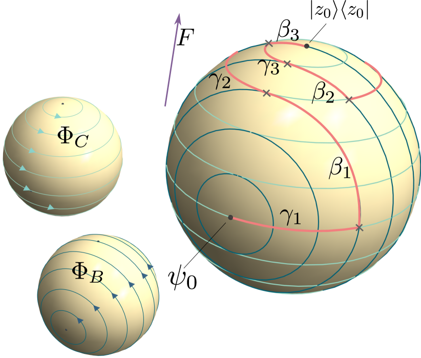
Performing a QAOA instance of depth with some parameters and hence can be understood in a nice geometrical picture: start from and follow (the flow of) the vector field for a distance given by parameter , stop and change direction to follow the (flow of the) vector field for a distance given by , and so on. Here the circuit depth determines the number of switching from one flow to the other. Situations in which shallow circuits suffice to reach a global minimum can therefore be associated to situations in which the vector fields have a simple structure (see, e.g., Figure 1). In converse, we expect that the, potentially exponential, hardness of a particular classical problem translates into a corresponding complexity of the vector field structure. Here the dimension of the corresponding Lie algebra would be a natural number for quantifying this.
2 The Lie Algebra of the Encoded Problem
For the characterization of optimization landscapes, we will first focus on the underlying manifold. Here, the central question is: which Lie group corresponds to a classical optimization problem encoded in a given Hamiltonian ? As the shape of a Lie group is fully encoded in its Lie algebra it already suffices to focus on this object. Here the above question translates to determining properties of the algebra which is generated by given operators and .
The precise form of might however be highly problem specific and will reflect the hardness of the underlying classical optimization problem becomes, in general, extremely hard to compute for large systems.
At this point, we will leave the detailed investigation of this connection for future work and instead provide statements on for a generic case.
Notably, it was prominently shown[19, 20] that almost every set of quantum logic gates with an action on more than one qubit can be used to generate any quantum circuit. A corresponding result for Lie algebras states that the algebra generated by randomly drawn traceless matrices almost certainly turns out to be the full algebra . This clearly suggests to ask for a similar behavior in the special case of the QAOA circuits.
Formally, we will say that the generators and of QAOA-gates are universal if . This follows automatically if the Lie algebra generated by and is . Clearly, this question has been investigated before[21] with the result that universality of QAOA circuits was proven for a wide range of objective Hamiltonians and their corresponding generator . The following theorem will contribute to this by a simple sufficient criterion for universality that can easily be checked by merely considering the possible values of the classical objective function . In the field of optimal control theory the notion of ‘controllability’ is the counterpart to the universality of a gate set in our case. Based on a convenient controllability criterion from [22] we get
Theorem 1.
and together form universal generators of QAOA-gates if the underlying classical optimization problem given by a target function fulfills the conditions
-
(a)
non-degenerate values:
-
(b)
non-degenerate resonance:
if ,
In particular, the set of optimization problems for which is open and dense (and hence the complement is a null set).
The proof of this theorem can be found in the Section VII. If one has , then it is always possible to solve the problem in finitely many steps, i.e., there exist , such that maps the initial state to a ground state of (see [23, Thm. 3.4]).
Thus, a randomly chosen optimization target will fulfill the criteria from Theorem 1 almost certainly, in which case we call severing. We can therefore draw the conclusion that universality is indeed a generic property of the QAOA. Generic instances of Knapsack, where the values and weights are arbitrary real numbers, or Traveling Salesman, where the distances between cities are arbitrary real numbers, (both encoded with soft constraints) will fall in this category. Furthermore, generic QUBOs are one of the classes for which universality was shown in [21].
Problem classes where values of are typically given by integers, like MAXCUT or MAX--SAT, do however not necessarily fulfill the conditions of Theorem 1 and could therefore lead to an optimization on smaller sets. If universality is a desired property, it can however always be restored by adding small perturbation. A concrete strategy would be to consider weighted MAXCUT or weighted MAX--SAT, with close to integer weights. The universality in these cases is ensured by the denseness statement in Theorem 1.
In general, it is however far from obvious whether a lack of universality is an obstacle or an actual feature. On one hand, we have that the reachable set becomes , the whole set of pure states when and thus, the largest possible search space. A smaller algebra would in turn lead to a smaller search space, which may make finding an optimum an easier task. However, on the other hand, a bigger algebra in principle also gives more paths that could be taken by the QAOA, which may in contrast enhance our chances to find short paths, which is one of the QAOA’s advertised features. Another feature of universality that we will explore in the following is that a sufficiently big algebra will prohibit the existence of local minima in the optimization landscapes. Here the intuition would be that a larger algebra provides us with more directions to move towards in order to escape from local extrema.
3 Classification of Critical Points
With the basic geometry set up in the previous subsections we can now turn our attention to our intended task of minimizing a target functional . As mentioned above, it is clear from the underlying manifold structure that the global minimum of on , the point we want to find, does not occur on any boundary. Hence, we will now follow the usual procedures for discussing the extreme points of a differentiable function. We start by considering critical points:
We call a critical point of provided that vanishes for all . It is clear that any minimum has to be within the set of critical points. Furthermore, the existence of critical points also plays a major role for the deep QAOA based on local optimization strategies. Here critical points typically appear as local attractors, which may impose major hurdles for a good overall performance. In the universal case, the critical points can be identified as the eigenstates of .
Proposition 2.
Let and be universal generators of QAOA-gates. Then the critical points of are precisely the eigenstates of .
Proof.
For an arbitrary and , it holds that
| (18) | |||||
Now is an eigenstate of if and only if the commutator vanishes. Thus, all eigenstates of that lie in are critical points. However, since we assume and to be universal, holds. Conversely, let vanish for all . Due to the assumed universality of and , we can choose and conclude that . Therefore, is already an eigenstate of . ∎
If the classical target function is severing, all eigenstates of are non-degenerate and therefore coincide with the computational basis states. Thus, we conclude
Corollary 3.
Let be severing. Then the critical points of are precisely the computational basis states.
The last proposition tells us, that the state we are looking for is a critical point of the functional. Moreover, there are no irregularities in terms of ‘hidden’ minima for some special functional.
4 Uniqueness of Minima and Maxima
Next, we want to go one step further and investigate properties of the second derivatives. These will allow us to distinguish between local minima, maxima, and saddle points. In fact, we have the following necessary condition for local extrema.
Corollary 4.
If is a local minimizer of then is a critical point of and for all , it holds that .
We call any critical point of with indefinite second derivatives saddle point. In the universal case, the critical points of are precisely given by the eigenstates of due to 2. This allows us to classify the local minima even further. Namely, local minima are already global ones.
Proposition 5.
Let and be universal generators of QAOA-gates. Then each local minimum of is already its global minimum and corresponds to a ground state of .
Proof.
By the Rayleigh-Ritz inequality, all global minima of correspond to ground states of . Let denote its ground state energy. Now, let be a local minimizer of . By 2 and 4, is an eigenstate of ; let denote the corresponding eigenvalue. Furthermore, for all , it holds that
| (19) |
If would not be a ground state of , one could choose so that is an (unnormalized) ground state of , implying that which clearly rises a contradiction. ∎
If the classical target function is severing, the degeneracy of the global minima is lifted and we obtain
Corollary 6.
Let be severing. Then admits its only local and global minimum at , where
In summary, a generic classical optimization problem, that is, with severing objective function , induces a very simple optimization geometry on : the critical points of precisely are the computational basis states and the only local and also global minimum is obtained at the state corresponding to the optimal solution to . Conversely, at any other point , we can always find a direction along which the functional strictly decreases. This simple structure is partially lost in the following chapter, where we only allow certain directions. The loss of information results in the appearance of additional local minima.
Our previous results are to be compared with [9]: While we show the absence of local minima in the state space landscape, they prove that certain VQA ansätze for MAXCUT result in local minimum-free parameter landscapes.
IV Deep Circuits
We will now discuss the regime of deep circuits. Here we consider local search routines on circuits with large but not fixed . For this, we can keep in mind an intuitive picture of what a local search does: In search of the minimum of , we maneuver through the state space landscape by small steps. In doing so, we are limited to only evaluate point-wisely and locally.
In contrast to the asymptotic regime from the previous section, we no longer assume that we can move in any direction from . In the explicit case of the QAOA, the remaining directions are and , since moving in any another direction, like for example , would in principle require an infinite sequence of infinitesimal gates.
Additionally, it is not guaranteed that all states from can be reached by circuits with a depth of reasonable order of magnitude.
1 Local Attractors and Traps
As a direct consequence of restricting search movements to the directions and , it can happen that we loose the ability of escaping from a saddle point. By this we effectively get new additional local minima when transiting from the asymptotic to the deep-circuit regime. As we will see, those can, in fact, be uncountable many.
As before we can identify local minima by looking at first and second derivatives in the available movement directions. Since stays constant under transformations in direction, we only have to consider directional derivatives in the direction . At a state those are given by
| (20) |
and
| (21) |
We substitute the operators and , as above, to shorten notations in the following. A state will turn into a local minimum for deep circuits if the second derivative is positive and the first derivative vanishes. This corresponds to a semi-definitely constrained set
| (22) |
Such a set will typically contain a full continuum of points. To get an intuition for this we can embed into the Hilbert-Schmidt space. Here, fulfilling the conditions for membership in (22) corresponds to the intersection of the state space with a high dimensional half space and a high dimensional subspace. Note that, in the generic case, will be disjoint. In the following, we will refer to its conjoint components as troughs. Our findings suggest that troughs are attracting regions for the QAOA with local search routines.
On a purely empirical level, we observe this behavior throughout our numerical studies. More details are given in Section V. On a theoretical level, a fully rigorous proof for this is unfortunately difficult to provide, since the full body of local search routines is hard to capture in a mathematical statement. We can, however, give some clear theoretical intuitions: By construction we have that, when starting from an arbitrary state , the minimization of along a trajectory , this is, only moving along direction , will end up in . For a very simple local search routine, this is indeed likely to happen, since following this direction will guarantee a monotonous descend. Performing movements in between might prevent this behavior. In this case the search routine may follow a more complicated path. If, at the end, this routine also minimizes gradients in the parameter landscape it will end up in , as well.
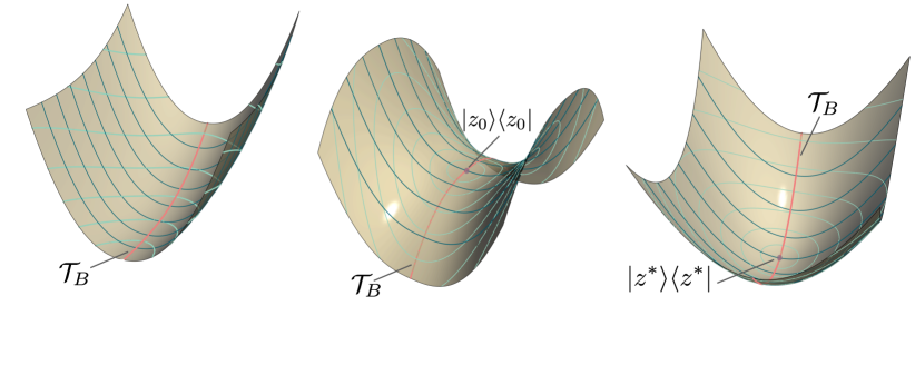
Once a search routine comes close to a trough a local search cannot leave the environment of a trough besides performing global movements (we will call them jumps). The behavior in such a situation is a forward and backward bouncing along the ‘walls’ of the trough. This is typical for local search routines and we also observe it throughout our numerical studies.
In the case of the QAOA an intuitive explanation for this can be given. Moving away from a trough by an movement will increase the value of and will hence be suppressed by a routine that looks for local optimally. We will therefore run into a circle in which movements into direction, which leave the value of invariant, are followed by a step in direction which moves back towards the trough. A usual problem in such situation is that, even though many steps are performed, the value of the functional will not, or only very slowly, improve. Even though refined routines like the conjugate gradient method[24] tend to avoid this behavior and adapting them for our special situation in the QAOA seems plausible, there are points within a trough where local search routines have to face further obstacles.
We recall from Section III that all non-optimal eigenstates of correspond to saddle points in the landscape. Here, first derivatives vanish such that those states are located in whenever their second derivative into direction is positive. Eigenstates of are also eigenstates of and by this have the property that they are invariant under movements. Additionally we also have that any point close to them will stay close under movements. We can see this by checking that the trace distance (which is unitarily invariant) between a state and an eigenstate stays constant along a trajectory, i.e. we have
| (23) |
As a result we observe that a local search around the eigenstates of that are also in will tend to get stuck. Due to the saddle point property, the functional will be almost constant, and no step allows to leave the region. We will mark those points as traps.
Let be an eigenstate of with eigenvalue . In order to decide if this state is in we have a consider its second derivative in direction. Using the computation in (19) we obtain
| (24) |
where denotes the Hamming distance between the two bit strings and . This expression has a nice interpretation. In the above, the sum
comes from the special form of that is characteristic for the QAOA. Up to a factor , it can be interpreted as the average of taken over all next nearest neighbors of in the hypercube . For what follows, it is useful to define the quantity
| (25) |
which can be understood as the average difference between the value of on and all neighboring strings. This average is proportional to the second derivative and suffices to determine what happens to the saddle point at when restricting to the deep-circuit regime.
Moreover, note that a string of length only has neighbors in . Therefore, the quantity can be efficiently determined by a classical computation that merely has to check and add the values of at those points.
2 Trap Sizes
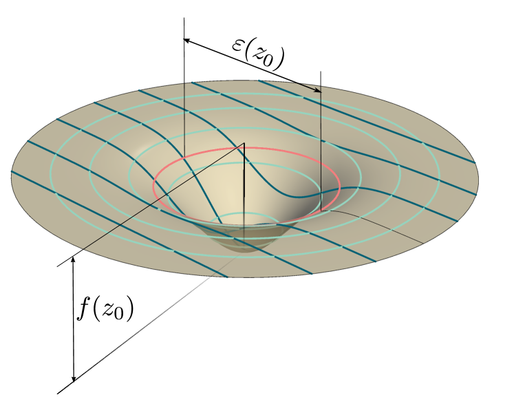
Once a local search is stuck in a trap, jumps, i.e. steps on a larger scale, have to be performed in order to escape. We can give an estimate on the required jump size by considering the distance from a trap to the closed state with negative second derivative. This, arguably heuristic, quantity will give us the scale on which the local behavior around a trap stops to dominate. See Figure 3 for a visualization. From now on, we will refer to a region around a trap in which all second derivatives are non-negative as valley.
Assume a trap centered at a state and an -neighborhood
By definition we can express any state in this neighborhood as
Thus, we can bound the second derivative of by the estimate
| (26) |
where we used Hölder’s inequality in the last step. Thus, by computing or estimating the universal factor for an explicit problem instance, one can estimate the size of a valley in the state space landscape by asking for all -neighborhoods in which all second derivatives are positive. From the last line of (26) we get a bound
| (27) |
on the critical .
Moreover, we can give an upper bound on by exploiting the sub-multiplicativity of the operator norm and eventually obtain
| (28) |
In combination with (27), we can conclude
| (29) |
This estimate has the natural interpretation, that the region around an eigenstate – especially around the global minimum – where one observes the same properties of the derivative as at the respective eigenstate gets smaller with growing problem size (). Furthermore, we can include the operator norm of into , by observing that in we can always consider normalized eigenvalues (with respect to the largest one). This yields a convenient redefinition
| (30) |
such that
| (31) |
Therefore, the properties of local minima with respect to depend only on the relative distances between the eigenvalues of as well as on the problem size .
3 A Performance Indicator
Valleys have an critical influence on the performance of deep-circuit QAOA as they are encompassing attractors and traps for local search routines. Intuitively, a landscape with ‘too many’ valleys, i.e. too many traps, seems to be unfavorable for a good performance. The previous section now employs us with tools for making such a statement more refined: In the following we consider the distribution of valleys with respect to their number, size, and depth. The statistics of these properties allow us then to identify obstacles for local search routines. By this we obtain an accessible performance indicator for deep-circuit QAOA.
Recall that the presence of a valley can be attested by the parameter , where shows that we have a valley with a radius (in trace distance) that can be estimated by (27). For a given target function , consider the set
| (32) |
From now on, we refer to a density plot of as the - diagram of . A lot of quantitative structure of the optimization landscape in state space can be directly observed from such a diagram. Several examples are given in Subsection 4.
Relevant question that can be directly answered by looking at a - diagram are:
-
(i)
What is the fraction of points with ?
-
(ii)
Are there correlations between the radius of a valley and its depth? Are the largest valleys also the deepest?
-
(iii)
Is there a separation between small and large valleys? Are large valleys less likely than small ones?
Quantitative answers to these questions allow us to estimate whether a landscape is in principle favorable or unfavorable for local search routines.
Generally a landscape with only few valleys (i) can be considered as favorable. Non-primitive routines for local search include subroutines for jumps that allow to escape a local trap and search for an optimum elsewhere. This can, however, only be performant if there are not too many traps. Without further structure given, we will assume that valleys with a large radius are more likely to attract a local search routine. Landscapes whose largest valleys are also the deepest ones (ii) can be considered as favorable, since here a local search is likely to find the global minimum of . One central aspect within the fine tuning of a local search routine is to adjust sizes of local steps and jumps. Here statistical information about the valley sizes (iii) can be very useful. In a favorable case, most valleys are small and shallow and only few valleys (including those we are looking for) are large and deep. Taking step sizes and jump sizes big enough will then allow us to fine tune a local search that effectively ignores small valleys and only gets attracted by large ones. In conclusion we will consider landscapes as favorable if the largest valley is also the deepest and the distribution of and thins out for increasing and decreasing , i.e. to the low-right corner of the - diagram. In the sense that it indicates the existence of performance obstacles, we mark the - diagram of a target objective as a two dimensional performance indicator.
Here we want to highlight once more that the - diagram only depends on data that can be obtained from only looking at classical efficiently accessible properties of on strings (the value of and its average on nearest neighbors). Hence statistical distribution properties can be estimated by a simple sampling of and over a set of randomly drawn strings.
On a more refined level, the task of assessing the unfavorability of a landscape translates into the task of estimating a tail distribution. This is a central task within the mathematical field of risk management [25] and many of the statistical methods developed there can be translated to our problem. At this point, however, we leave a detailed analysis and application of those methods for future work and restrict, for the moment, to the provision of examples.
4 Examples
A central question for the assessment of the perspectives of QAOA is to spot instances and problem classes in which an algorithm has a chance for a good performance. However, one has to expect the existence of ‘no free lunch’- theorems implying that most instances will not perform well.
We immediately observe such a behavior when considering objectives in which the values of are distributed without paying attention to the topology of .
Examples are given in LABEL:figure:MuFRandom. Here we first generated the values of according to a distribution function, and then assigned them with uniform randomness to bit strings. In the first example, is also uniformly distributed over the interval leading to an unfavorable landscape in which the valley sizes are uniformly distributed, as well. In the second example from LABEL:figure:MuFRandom, we distribute the values of with respect to a bi-modal distribution that favors large and small values. Here, a ‘no free lunch’ behavior clearly reveals by the fact that the global minimum has no distinct statistical properties with respect to a substantial amount of the local traps.
This situation changes when we consider random instances of QUBO, i.e. functions of the form
| (33) |
generated from a randomly chosen hermitian matrix with unit norm. Here, we have that the values of on neighboring strings have a mutual dependence. A corresponding - diagram is shown in Figure 5.
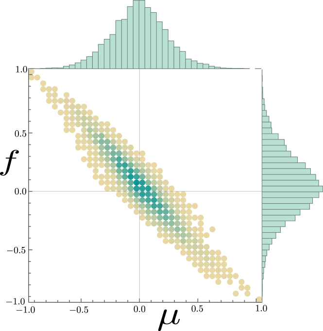
We observe a thin tail and hence a favorable landscape. In correspondence we also see from our numerical studies that already a local search with a simple downhill simplex method performs better on those instances. We expect that this tail behavior can be explained by employing the central limit theorem. However, we leave a full proof for future work. When going through the catalogue of special classes of pseudo Boolean functions[26] one can immediately spot further classes that admit a favorable landscape. One of those are functions that are zero on almost all strings, and negative on only very few of them. Here, the landscape is mostly flat, and all valleys will encompass a global minimum. For example, SAT problems with only few feasible points would constitute such functions. Remarkably those are in close correspondence to the ‘find the marked entry in a database’ problem Grover’s search algorithm[27] solves with a proven quantum speedup.
V Numerical Results
In the previous sections we elaborated on several aspects of the interplay between local search routines and the geometry of the state space optimization landscape. In this section we will employ a simple local search routine to demonstrate these on concrete examples.
At this stage we will obtain our results by numerically simulating the behavior of a noise-free quantum computer. Observations inferred from this clearly over-idealized setting therefore only account for ruling out the feasibility of a problem instance and not for ultimately demonstrating it.
Rather than using Qiskit or similar existing frameworks, we perform simulations on the level of explicitly implementing the matrices and vectors involved. By this all major computations can be directly performed by matrix-vector multiplications in an optimized library, such as BLAS. We thus guarantee that the run-time of our simulations scales linearly with the circuit depth , and can therefore simulate very deep circuits within fractions of a second.
1 A Basic Local Search Algorithm
For the numerical studies of this section, we employ a very simple and entirely naive local search routine which could be referred to as state space versions of pattern search[28] or random search[29, 30]. It works as follows:
-
0.
Fix an initial state and a set of unitaries and start with .
-
1.
For , create states .
-
2.
Measure the target Hamiltonian on the states , i.e. compute
-
3.
Pick , set as active estimate, set and go to
If all are close to the identity this will generate a simple local search routine. Here, the step size in statespace is determined by the difference between the and the identity evaluated on an active state . An upper bound to this distance is given by taking the maximal operator norm distance between the and the identity. For our concrete examples we take the to be one layer of QAOA unitaries with parameter tuples taken from a grid-like pattern around zero. The maximum size of the grid is , and the points in it are equally spaced into steps for and steps for . For small , and by setting , the parameter corresponds, at least approximately, to an upper bound on the actual step size in statespace. In any case, can be regarded as an effective size parameter that determines a characteristic scale on which the local search routine above performs its work.
It is important to point out that our main intention for employing this type of algorithm is to investigate the basic behavior of local search routines and not to achieve anything close to the best possible performance. Search algorithms of a type as the above usually give a high robustness for successively improving the estimate on an optimization target without requiring a lot of preconditioning on a particular problem instance. This, however, typically comes at the price of performing many optimization rounds. In order to achieve a good convergence speed more refined algorithms and a lot of case-to-case feature engineering will be required.
2 Description of Depicted Data
For our numerical studies we run the above algorithm on various exemplary instances. Characteristic information on a particular run of this algorithm is gathered by depicting:
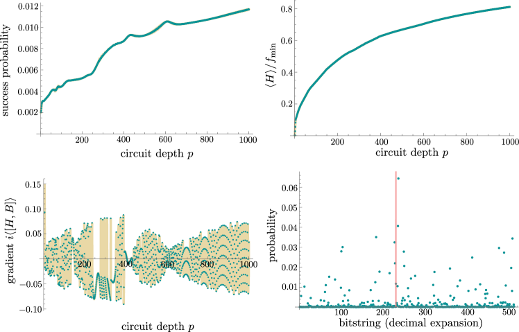
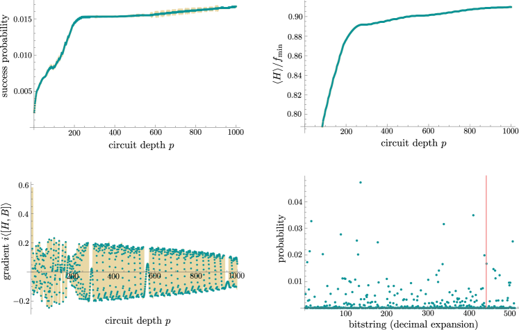
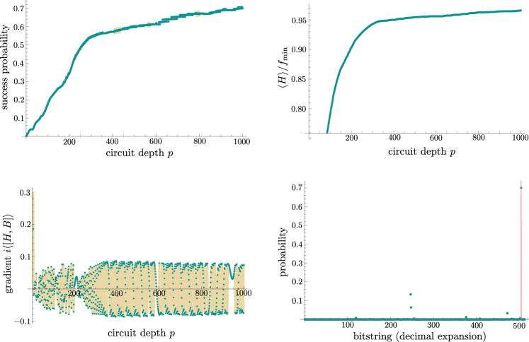
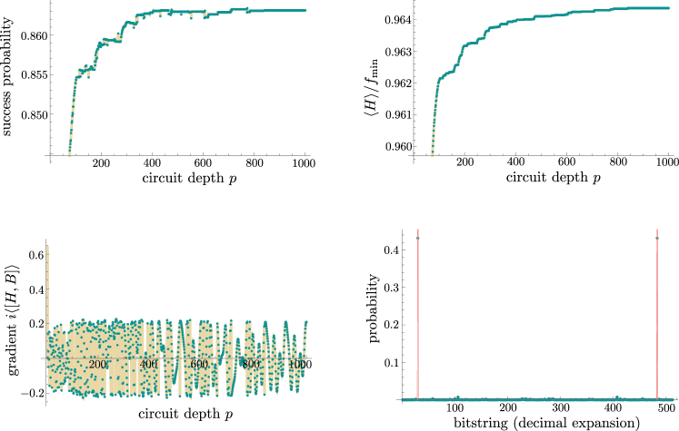
-
(i)
the success probability of obtaining the optimal outcome string of a particular optimization problem obtained by measuring the target Hamiltonian on the respective active state . This will be depicted as a function of the circuit depth , i.e. the number of rounds the algorithm was performed.
-
(ii)
the outcome probability distribution of strings obtained by measuring the final active state in the computational basis. The bit strings are converted into the decimal system. The red line in each of these plots marks the location of the optimal solution(s) of a given optimization problem.
-
(iii)
the approximation ratio obtained by measuring the target Hamiltonian on the active state ; again as a function of the number of optimization rounds.
-
(iv)
the size of the gradient of the functional along an trajectory, evaluated at the active state ; again as a function of the number of optimization rounds.
3 Performance of Deep-Circuit Local Search
In this subsection, we verify the significance our just introduced performance indicator, the - diagram, on examples. First, we study the performance of the above algorithm for a function with uniformly randomly distributed values on . For the step size we use . In contrast to LABEL:figure:MuFRandom, the function is defined on bit strings of length nine instead of 13. However, we observe, qualitatively, exactly the performance behavior that is predicted by the - diagram for the larger instance (see Figure 7): Even after 1000 iterations the success probability of approximately is comparatively small. Accordingly, the final outcome distribution is smeared out with no significant peak around local or global minima. The approximation ratio seems to slowly increase proportionally to . Furthermore, the gradient oscillates as a function of with slowly oscillating amplitude.
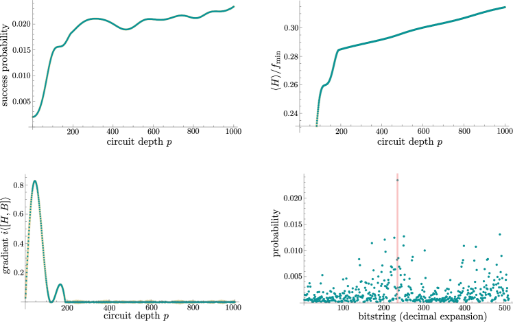
Second, we consider a concrete numerical example of a function with bimodally randomly distributed values on , again with a step size of . Again, we choose a nine-bit example which qualitatively admits the properties predicted by the - diagram of the corresponding larger instance (see Figure 8): After 1000 iterations the success probability is approximately and thus again comparatively small. The final outcome distribution is as smeared out as in the uniform case. This time, however, we observe a different behavior of the approximation ratio. It rapidly increases within the first 300 iterations and seems to be saturated thereafter, subsequently resulting in a very slow increase. The gradient again oscillates as a function of with a slowly decreasing amplitude.
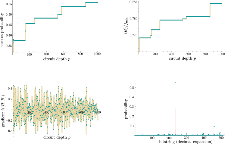
We next investigate a random QUBO function on 9 bits, also with a moderate step size of . The - diagram of its 13-bit counterpart (Figure 5) predicts a favorable landscape. This is exactly what we observe in the numerical data (see Figure 9): The success probability increases up to over the course of 1000 iterations and is thus significantly higher than in both preceding examples. Accordingly, the final outcome distribution strongly concentrates around the optimal solution. The approximation ratio behaves similarly to the bimodal case, that is, it rapidly increases at first and then saturates. In the QUBO case, however, the saturation occurs at a higher ratio. The gradient also behaves similarly to the bimodal case, regarding both its oscillation and its amplitude.
In addition, we consider a more concrete example: a MAXCUT instance for a random graph with nine vertices and unweighted edges (Figure 6).
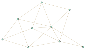
The resulting objective function is also of QUBO-type and we therefore expect a favorable optimization landscape. However, the function merely is integer-valued. Furthermore, it is symmetric under flipping each bit of its argument. Therefore, the criteria of Theorem 1 are not met and it is thus of particular interest whether our performance indicator, the - diagram, still applies. Indeed, our numerical results (step size ) indicate a favorable landscape (see Figure 10): After iterations, the success probability even exceeds that of the previous QUBO instance by roughly . Likewise, the final outcome distribution strongly concentrates around the two optimal solutions. We again observe a saturation of the approximation ratio after 300 steps, but with an even higher saturated ratio than in the previous case. The gradient also admits oscillations in , but its overall amplitude is doubled in comparison to the previous case.
4 Local Traps
The existence of local traps plays a central role for the success chances of a local search routine. Recall from the previous section that traps for local search routines are precisely located at the eigenstates of the target Hamiltonian.
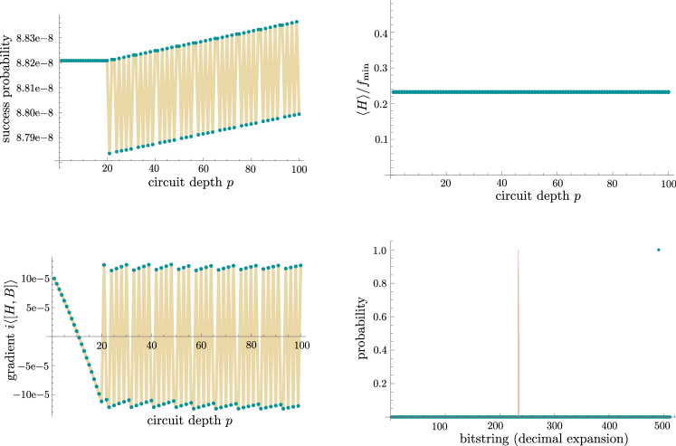
As outlined in Subsection 1 those traps effectively arise from saddle points in the asymptotic landscape from which a low layer optimization can not escape due to the fact that the moves in directions needed for this demand unitaries with long circuits. We observe this behavior throughout our numerical studies. This time, we intentionally start at a state that is close to a non-optimal eigenstate of a Hamiltonian that corresponds to a random instance of QUBO on 9 qubits. We used the algorithm from Subsection 1 with a small () effective step size parameter. We terminate the algorithm after 100 rounds, since the results already indicate that our search does effectively not leave the environment of the non-optimal eigenstate close to which we started (see Figure 11). The probability distribution of outcomes obtained from the last state has all its weight on a single point which corresponds to . The approximation ratio stays constant at the value of . A more refined behavior can be inferred from the success probability and the gradient which are both depicted on a very fine scale. For the first 20 steps the success probability stays constant and the gradient slowly decreases. Afterwards the gradient and the success probability begin to oscillate. While the gradient stays small, the success probability begins to grow linearly. Both effects happen on a very small scale, i.e., the gradient stays almost zero and the linear growth is almost flat. Even thought the effective step size was on order the slope of the success probability is much smaller, namely on the order of . Therefore, the algorithm is effectively trapped.
5 Step Size Analysis
For the same random QUBO function as before, we further investigate the algorithmic behavior for two different step sizes . The small step size results in a very slow traversing of the favorable landscape (see Figure 12): The success probability evolves in the same way as it does for the previously considered QUBO instance with moderate step size. However, the scale on which it is increasing is drastically smaller. Accordingly, the final outcome distribution is smeared out as in the case of an unfavorable landscape. Due to the slow movement, the approximation ratio does not reach its saturation during the first 1000 iterations. It rather admits a shallow linear increase over a wide range of iterations. In addition, the gradient admits, after an initial burst, a very small amplitude, indicating again the slow motion through the optimization landscape.
Meanwhile, the large step size results in a completely different behavior (see Figure 13): The success probability stays constant throughout large periods of iterations and admits jumps between these plateaus. After 1000 iterations, it reaches a considerably large value of . This corresponds to a strong concentration of the final outcome distribution around the optimal solution. The approximation ratio stays constant throughout the same iteration intervals as the success probability with jumps in between. We also observe that the gradient is strongly oscillating with a comparatively large amplitude which directly follows from the large step size.
VI Outlook and Conclusion
This work is done under the impression that technological advances of the NISQ era might reach a next stage in a not too far future. For this we share the aspirations that quantum computing with deep circuits will become practically feasible. In this regime the quantum-classical ansatz of variational quantum computing will likely keep its popularity. Estimating perspectives of practical applicability, spotting new obstacles, and finding promising problem classes is therefore a relevant quest that can already be started today.
By this work we contribute to the collection of methods, tools, and structural insights that will hopefully lead to a better understanding on why the QAOA practically fails in many examples and when it could in principle work.
As we have seen, regarding optimization landscapes from a state space perspective allows for a clear analysis that reveals rich but still accessible mathematical structures. This has to be seen in clear contrast to the, in some extend, more often employed perspective on optimization landscapes in the parameter space of . The mapping from does not really respect the natural topology of the problem. Several, apparently different, local minima and traps in parameter space could for example correspond to one and the same local minimum in state space. In this sense obstacles that are spotted in the state space picture give us a clear hint towards the persistent geometric core of the underlying problem.
We expect that the analysis of the - diagrams, which we introduced as a performance indicator, will turn out as a useful tool for future research. By considering only few basic examples, we merely scratched on the surface of its applicability. Analyzing this indicator and evaluating its impact for practical problem instances will be an essential task for future research.
From the results we have seen so far, it becomes however already clear that there will be no universal applicability of QAOA in deep circuits. We see that problem instances that avoid unfavorable landscapes must have a specialized underlying structure and are presumable rare. This is totally in line to the typical observation that no method ever gives a ‘free lunch’.
Lastly, we have to point out that many further aspects, that influence the performance of a local search, have been neglected in this work. This especially includes the actual circuit depth required for approximating the solution of a problem up to a convincing ratio. For local search routines this depth can be highly problem-specific and might drastically vary with respect to the explicit method in use. Finding good routines will most likely demand a lot of explicit feature engineering. Even though we found some promising simple examples in our numerical studies, a conclusive assessment of instances with favorable landscapes can very likely reveal further obstacles.
Acknowledgments
We thank Daniel Burgarth, Tobias J. Osborne, Antonio Rotundo, Bence Marton Temesi, Arne-Christian Voigt, Reinhard F. Werner, and Sören Wilkening for helpful discussions. GK acknowledges financial support by the DAAD and IIT Indore (Kapil Ahuja) for a guest stay. LvL and RS acknowledge financial support by the Quantum Valley Lower Saxony. RS acknowledges financial support by the BMBF project ATIQ. LB and TZ acknowledge finanical support by the BMBF project QuBRA.
References
- Cerezo et al. [2021] M. Cerezo, A. Arrasmith, R. Babbush, S. C. Benjamin, S. Endo, K. Fujii, J. R. McClean, K. Mitarai, X. Yuan, L. Cincio, and P. J. Coles, Nature Reviews Physics 3, 625 (2021).
- Farhi et al. [2014] E. Farhi, J. Goldstone, and S. Gutmann, A Quantum Approximate Optimization Algorithm (2014), arXiv:1411.4028 [quant-ph] .
- Harrigan et al. [2021] M. P. Harrigan et al., Nature Physics 17, 332 (2021).
- Willsch et al. [2020] M. Willsch, D. Willsch, F. Jin, H. D. Raedt, and K. Michielsen, Quantum Information Processing 19, 197 (2020).
- Crooks [2018] G. E. Crooks, Performance of the Quantum Approximate Optimization Algorithm on the Maximum Cut Problem (2018), arXiv:1811.08419 [quant-ph] .
- Lykov et al. [2022] D. Lykov, J. Wurtz, C. Poole, M. Saffman, T. Noel, and Y. Alexeev, Sampling Frequency Thresholds for Quantum Advantage of Quantum Approximate Optimization Algorithm (2022), arXiv:2206.03579 [quant-ph] .
- Bravyi et al. [2020] S. Bravyi, A. Kliesch, R. Koenig, and E. Tang, Physical Review Letters 125, 260505 (2020).
- Hastings [2019] M. B. Hastings, Classical and Quantum Bounded Depth Approximation Algorithms (2019), arXiv:1905.07047 [quant-ph] .
- Lee et al. [2021] J. Lee, A. B. Magann, H. A. Rabitz, and C. Arenz, Physical Review A 104, 032401 (2021).
- Note [1] The original QAOA is formulated for maximization tasks; here is defined with the opposite sign.
- Endo et al. [2018] S. Endo, S. C. Benjamin, and Y. Li, Physical Review X 8, 031027 (2018).
- Egan et al. [2021] L. Egan, D. M. Debroy, C. Noel, A. Risinger, D. Zhu, D. Biswas, M. Newman, M. Li, K. R. Brown, M. Cetina, and C. Monroe, Nature 598, 281 (2021).
- Larocca et al. [2022] M. Larocca, P. Czarnik, K. Sharma, G. Muraleedharan, P. J. Coles, and M. Cerezo, Quantum 6, 824 (2022).
- McClean et al. [2019] J. R. McClean, S. Boixo, V. N. Smelyanskiy, R. Babbush, and H. Neven, Nature Communications 9, 4812 (2019).
- Campos et al. [2021] E. Campos, A. Nasrallah, and J. Biamonte, Physical Review A 103, 032607 (2021).
- Ge et al. [2022] X. Ge, R.-B. Wu, and H. Rabitz, The Optimization Landscape of Hybrid Quantum-Classical Algorithms: from Quantum Control to NISQ Applications (2022), arXiv:2201.07448 [quant-ph] .
- Note [2] This is clear for finite circuits, for infinite circuits the proper limits have to be taken into account.
- Note [3] On an abstract level we can consider as a subgroup of . Here Cartan’s theorem on closed-subgroups[31] states that the embedding of into the smooth structure of will give us a consistent smooth structure on itself.
- Lloyd [1995] S. Lloyd, Physical Review Letters 75, 346 (1995).
- Deutsch et al. [1995] D. Deutsch, A. Barenco, and A. Ekert, Proceedings: Mathematical and Physical Sciences 449, 669 (1995).
- Morales et al. [2020] M. E. S. Morales, J. D. Biamonte, and Z. Zimborás, Quantum Information Processing 19, 291 (2020).
- Altafini [2002] C. Altafini, Journal of Mathematical Physics 43, 2051 (2002).
- Agrachev and Sachkov [2004] A. A. Agrachev and Y. L. Sachkov, Control theory from the geometric viewpoint, Vol. 2 (Springer Science & Business Media, 2004).
- Shewchuk [1994] J. R. Shewchuk, An Introduction to the Conjugate Gradient Method Without the Agonizing Pain, Tech. Rep. (USA, 1994).
- Baker and Radha [2022] J. S. Baker and S. K. Radha, Wasserstein Solution Quality and the Quantum Approximate Optimization Algorithm: A Portfolio Optimization Case Study (2022), arXiv:2202.06782 [quant-ph] .
- Crama and Hammer [2011] Y. Crama and P. L. Hammer, Boolean Functions Theory, Algorithms, and Applications (Cambridge University Press, 2011).
- Grover [1996] L. K. Grover, A fast quantum mechanical algorithm for database search (1996), arXiv:9605043 [quant-ph] .
- Hooke and Jeeves [1961] R. Hooke and T. A. Jeeves, Journal of the ACM (JACM) 8, 212 (1961).
- Anderson [1953] R. L. Anderson, Journal of the American Statistical Association 48, 789 (1953).
- Brooks [1958] S. H. Brooks, Operations research 6, 244 (1958).
- Lee [2003] J. M. Lee, Introduction to Smooth Manifolds, Vol. 218 (Springer New York, NY, 2003).
- Zeier and Schulte-Herbrüggen [2011] R. Zeier and T. Schulte-Herbrüggen, Journal of mathematical physics 52, 113510 (2011).
- Zeier and Zimborás [2015] R. Zeier and Z. Zimborás, Journal of Mathematical Physics 56, 081702 (2015).
- Zimborás et al. [2015] Z. Zimborás, R. Zeier, T. Schulte-Herbrüggen, and D. Burgarth, Physical Review A 92, 042309 (2015).
VII Appendix
Proof of Theorem 1.
Given Hermitian operators and on a (finite dimensional) Hilbert space , under what conditions is the generated Lie algebra equal to ? This question is particularly important in the field of control theory and has, for example, been looked at in [22, 32, 33, 34]. We will use the sufficient condition in [22, Theorem 2] stating that if is strongly regular (which is equivalent to our assumptions (a) and (b)) and if the graph of is connected (see below), then , or equivalently .
The graph of an operator is defined with respect to a basis as follows: The vertices of are the different basis labels and there is an oriented edge joining and if and only if . That is, the matrix representation of in the same basis is, up to normalization of its entries, the adjacency matrix of the graph . However, since , as a matrix in the computational basis, is irreducible[2], we readily optain that its graph is connected. ∎