Target Aware Poisson-Gaussian Noise Parameters Estimation from Noisy Images

Abstract

Digital sensors can lead to noisy results under many circumstances. To be able to remove the undesired noise from images, proper noise modeling and an accurate noise parameter estimation is crucial. In this project, we use a Poisson-Gaussian noise model for the raw-images captured by the sensor, as it fits the physical characteristics of the sensor closely. Moreover, we limit ourselves to the case where observed (noisy), and ground-truth (noise-free) image pairs are available. Using such pairs is beneficial for the noise estimation and is not widely studied in literature. Based on this model, we derive the theoretical maximum likelihood solution, discuss its practical implementation and optimization. Further, we propose two algorithms based on variance and cumulant statistics. Finally, we compare the results of our methods with two different approaches, a CNN we trained ourselves, and another one taken from literature. The comparison between all these methods shows that our algorithms outperform the others in terms of MSE and have good additional properties.

I Introduction

Every image capturing system is inherently noisy. The noise is influenced by different factors and different systems have different noise characteristics. In our project, we pick a model of noise having two components, one being a Poisson distribution and the other one a Gaussian.

Roughly, capturing an image can be seen as the process of counting the number of incident photons that hit a sensor pixel during a given amount of time. More photons in a given interval of time translates to more light and hence more intensity for the pixel of the final image. Hence, the Poisson distribution is inherent to that discrete photon counting phenomenon. The Poisson contribution in that context is commonly referred to as photon shot noise. The second element of our noise model, the Gaussian, is introduced by a collection of different error factors like the quantum efficiency, the circuitry, unwanted interactions between pixels, read out errors and many more. Overall, all those error sources combined can be modeled with a single Gaussian.

Our goal is to estimate the parameters of this noise model. Knowing those values enables performing noise correction. More precisely, from an observed noisy image, $y$ reconstruct the ground-truth image $x$. In our setting, we assume to have access to both $y$ and $x$. This assumption is reasonable in a calibration setting where one can do long exposure times to minimize the Poisson contribution and average over several images to reduce the impact of the Gaussian noise part. Once calibrated (i.e., having estimated the noise parameters) newly captured images (without knowing the ground-truth) can be corrected for the noise leading to better results.

Generally, there are two main approaches to noise estimation today, either using statistical techniques and signal processing or deep learning. The former involves more domain specific knowledge.

The method presented by Foi et al. [1] follows the ideas of the first approach. Additionally, it uses a Poisson-Gaussian noise model like we do but only uses observations of the noisy signal, not the ground-truth $x$. Hence, the problem the authors of [1] try to solve is inherently more difficult than ours. In our setting we have knowledge of both $y$ and $x$, hence, this advantage should enable us to achieve better performance.

On the other hand, deep learning is increasingly often applied to all kinds of fields, noise estimation is no exception. Specifically, Convolutional Neural Networks (CNN) that are abundantly used in many image related tasks. Here, we are not limited to using only $y$ but also $x$ and maybe even $|y-x|$

In this project, we propose novel methods of noise estimation while comparing their performance to different approaches. Further, we put those results into perspective by providing the log-likelihood we derived for this problem.

In the case where both $x$ and $y$ are at hand, our findings allow improving over the conventional methods.

For our method to work, we heavily rely on the knowledge of the noise-free ground-truth image $x$. Further, we are only working with grayscale images, but our methods are extendable to multichannel images. Each channel’s noise parameters might be different from each other, as each channel is independent from any other. Additionally, we didn’t address the issue of clipping, i.e., handling values that lay outside the range of valid pixel intensities. For instance, intensity is given by a value in $[0.,1.]$ and any pixels’ intensity beyond this interval should be clipped to it’s closest bound of the interval in order for it a valid value. But clipping is introducing a nonlinearity which makes all the derivations we make more complex. For simplicity, we allowed values to exceed the range and do not apply any clipping.

II Related work

Denoising is one of the most fundamental tasks in image restoration, with both theoretical impact and practical applications. Most classic denoisers, for instance PURE-LET [2], KSVD [3], WNNM [4], BM3D [5], and EPLL [6], require knowledge of the noise level in the input test image. Deep learning image denoisers that have shown improved empirical performance [7, 8] also require knowledge of noise distributions, if not at test time [9], then at least for training [10, 11]. This is due to the degradation overfitting of deep neural networks [12]. Noise modeling is thus important for denoisers at test time, but also for acquisition system analysis and dataset modeling for training these denoisers. Past research has focused on modeling noise from noisy images without relying on ground truth, i.e., noise-free, information [1]. Interesting approaches, for example Sparse Modeling [13], Dictionary Learning [14] or non-local image denoising methods like SAFPI [15], have been developed to push overall denoising performance. However, none of these methods allow easy use of noise-free data when it is available. For Poisson-Gaussian noise modeling, for example, both FMD [16] and W2S [17] rely on a noise modeling method that does not consider ground truth noise-free images [1]. Hence, our approach to model the Poisson-Gaussian Image Noise (PoGaIN) distribution exploits paired samples (noisy and noise-free images), which significantly improves the modeling accuracy. Our method is based on the cumulant expansion, which is also used by other authors to derive estimators for PoGaIN model parameters, but for different input types, such as noisy image time series [18] or single noisy images [19]. We lastly refer the reader to our concise publication that sums up the essential elements of this report [20].

III Theory

III-A Poisson-Gaussian Modeling

The generic signal-dependent Poisson-Gaussian noise modeling can be written as the following form :

$$y=\frac{1}{a}\alpha+\beta,\quad\alpha\sim\mathcal{P}(ax),\quad\beta\sim\mathcal{N}(0,b^{2})$$ (1)

where $x$ is the known ground-truth signal and $y$ is the observed signal. In our modeling, Poisson signal-dependent component $\eta_{p}$ and Gaussian signal-independent component $\eta_{g}$ are defined as,

$$\eta_{p}=\frac{1}{a}\alpha,\quad\eta_{g}=\beta$$ (2)

where these two components are assumed to be independent. From the derivation given in Appendix -A, the following properties of the observed signal, $y$, can be found :

$$\mathbb{E}[\eta_{p}]=x,\quad\mathbb{V}[\eta_{p}]=\frac{x}{a}$$ (3)

Here, the fact that Poisson noise has signal-dependent characteristics. On the other hand, the Gaussian noise has the constant variance and mean, which makes it signal independent as expected. Consequently, the following equation 4 is obtained.

$$\mathbb{E}[y]=x,\quad\mathbb{V}[y]=\frac{x}{a}+b^{2}$$ (4)

Intuitively, it means that the average of the observed image should be the ground-truth image, which justifies the reasoning. From the variance equation, the fact that variance is affected directly by $a$ and $b$ makes it reasonable as they represent the noises.

III-B Raw-Data Modeling

Poisson-Gaussian model is properly matched with the natural characteristics of raw-data of digital imaging systems. The Poisson noise models the signal-dependent part of errors, which are caused by the discrete nature of the photon-counting process. On the other hand, Gaussian noise models the signal independent errors, such as electric and thermal noise.

The parameter of the Poisson noise, $\alpha$ is dependent on the quantum efficiency of the sensor. The more the number of photons to generate the electrons inside the sensor is, the less the value of $\alpha$ is. According to experiments conducted by [21], this Poisson noise effect can be the dominant contributor to uncertainty in the raw data captured by high-performance sensors. This justifies the accuracy of the modeling for raw-image of the sensors.

Analog gain which is the amplification of the collected charge in the digital imaging systems is another dependent that affects both Poisson and Gaussian noise parameters. In digital camera, it is controlled by ISO and/or exposure index (EI) sensitivity settings. The larger the ISO number is, the larger analog gain resulted in, which causes the amplification of the noises as well. This causes the decrease in SNR of the captured raw-data, which means the noise increases. We can conclude that both of the noise parameters can be highly dependent on the analog gain.

In the case of the system with large photon counting condition, Poisson noise can be approximated as Gaussian noise as the following.

$$\mathcal{P}(\lambda)=\mathcal{N}(\lambda,\lambda)$$ (5)

This approximation can be useful for deriving the solution based only on mean and variance, which simplifies the process of proposing algorithms without using ground-truth image [1]. However, since we were also looking for the method that uses the ground-truth image as input, this approximation is not applied for the following sections. Another reason is that this approximation results in the loss of information about the statistics of the actual noise parameters. In other words, it results in lossy projection of $a$ and $b$ into less dimensional space, which is not desirable.

III-C Maximum Likelihood Solution

When the noise modeling in equation 1 is applied to a raw-data image, the following likelihood function of the pixel intensity of an observed image can be achieved with the derivation explained in Appendix -A.

$$f_{y}(y_{n}|a,b,x)=\sum_{k=0}^{\infty}\frac{(ax_{n})^{k}}{k!b\sqrt{2\pi}}\exp{\left(-ax_{n}-\frac{(y_{n}-k/a)^{2}}{2b^{2}}\right)}$$ (6)

where $y$ is observed image, $x$ is the ground-truth image and $n$ is the pixel index.

In order to propose a robust noise parameter estimation algorithm, the optimality criterion is chosen to be the maximization of the likelihood function in  6 with respect to noise parameters, $a$ and $b$. The resulted solution of this optimality criterion is called as Maximum Likelihood solution. From the derivation in -A, the following solution is found.

$$\begin{split}\hat{a},\hat{b}=\arg\max_{a,b}\prod_{n}\sum_{k=0}^{\infty}\frac{(ax_{n})^{k}}{k!b\sqrt{2\pi}}\exp{\left(-ax_{n}-\frac{(y_{n}-k/a)^{2}}{2b^{2}}\right)}\end{split}$$ (7)

IV Implemented Methods

IV-A Grid Search for ML Solution

Maximum Likelihood solution offers an accurate estimation of the noise parameters in theory. However, for the practical reasons, it’s hard to propose the algorithmic solution for the maximization of the functional inside the ML solution. This functional in equation 7 is analyzed and found to be non-concave. Thus, gradient-based optimization algorithms cannot be applied for this maximization problem. For the sake of implementation of ML solution, the most naive method is proposed to estimate the noise parameters $a$ and $b$. This is also possible, as we only have two parameters to be estimated.

As an implementation issue, exact calculation of likelihood function is difficult as it includes infinity sum as seen in equation 6. In order to approximately estimate it, a sufficiently large value of $k_{max}$ is chosen, and the following is applied:

$$f_{y}(y_{n}|a,b,x)\approx\sum_{k=0}^{k_{max}}\frac{(ax_{n})^{k}}{k!b\sqrt{2\pi}}\exp{\left(-ax_{n}-\frac{(y_{n}-k/a)^{2}}{2b^{2}}\right)}$$ (8)

However, from the analysis of the non-concavity behavior of the likelihood function, it’s found that it does not result in sufficiently good results for the estimation of noise parameters. In order to achieve the accurate results, very small step sizes should be chosen. This makes the algorithm computationally too expensive to be solved in practice, and it is justified by the testings.

Therefore, in this project, we present and compare three different methods from ML solution to estimate the parameters of the Poisson-Gaussian noise. The first method is based on the variance of the noisy image for each pixel value of the real image. Then, we will present a method based on the cumulant of the noisy image and the knowledge we have of the real image. Finally, we implemented a basic convolution neural network in order to compare our result.

IV-B Variance

This method is based on the variance of the values of the noisy image for a fixed intensity of the real image. That is to say, we take a pixel $i$ from $x$ of intensity $x_{i}$, then for every $j$ such that $x_{j}=x_{i}$, we have $y_{j}\sim\frac{\mathcal{P}(ax_{i})}{a}+\mathcal{N}(0,b^{2})$. Thus, if we denote $Y_{i}=\set{y_{k}:x_{k}=x_{i}}$, we have $\mathbb{V}[Y_{i}]\approx\frac{x_{i}}{a}+b^{2}$. We can calculate this variance with each distinct value of $x_{i}$. In our case, images are saved in 8-bits, thus we only have 256 unique different values of $x_{i}$. Moreover, as we know the theoretical mean of $Y_{i}$ is $x_{i}$, we can calculate the variance using :

$$\mathbb{V}[Y_{i}]=\frac{1}{\left|Y_{i}\right|}\sum_{y_{k}\in Y_{i}}(y_{k}-x_{i})^{2}$$ (9)

Finally, to obtain the estimation of $a,b$ is :

$$\hat{a},\hat{b}=\arg\min_{a,b}{\sum_{i}(\mathbb{V}[Y_{i}]-\frac{x_{i}}{a}-b^{2})^{2}}$$ (10)

Note that in equation 10, the same point $(x_{i},\mathbb{V}[Y_{i}])$ is present $\left|Y_{i}\right|$ times. This is because we found better result using this bias. This method has multiple default, first it is not unbiased, then it works best on images with a small amount of unique pixel intensities but an important difference between the minimum and maximum intensity. Also, because it is biased, this method can be tuned to be better (for instance, the importance of each terms on the right side of equation 10 can be modified so that higher values of $x_{i}$ has a smaller weight).

IV-C Cumulant

This method uses the cumulant expansion of the noisy image. In this section, instead of seeing $x$ and $y$ as images, we see $x$ and $y$ as samples from a distribution where $x\sim\mathcal{X}$ and $y\sim\mathcal{Y}$ such that :

$$\mathbb{P}[x=x_{i}]=\frac{\left|\set{k:x_{k}=x_{i}}\right|}{n}$$

where $n$ correspond to the number of sample (i.e., the size of $x$ and $y$). Then we can define $\mathcal{Y}$ as the distribution of Poisson-Gaussian noise over the distribution $\mathcal{X}$. Formally:

$$\mathcal{Y}\sim\frac{\mathcal{P}(a\mathcal{X})}{a}+\mathcal{N}(0,b^{2})$$ (11)

We then use the equation 12 calculated in appendix -B to get the cumulant of $\mathcal{Y}$ as a system of two equations :

$$\begin{split}\kappa_{2}&=\frac{\overline{x}}{a}+\overline{x^{2}}-\overline{x}^{2}+b^{2}\\ \kappa_{3}&=\overline{x^{3}}-3\overline{x^{2}}\overline{x}+2\overline{x}^{3}+3\frac{\overline{x^{2}}}{a}-3\frac{\overline{x}^{2}}{a}+\frac{\overline{x}}{a^{2}}\end{split}$$ (12)

where $\overline{x^{k}}^{j}=(\frac{1}{n}\sum_{i}x_{i}^{k})^{j}$. Equations 12 forms a system of two equations with two variables : $a$ and $b$, the parameters of the noise. This method benefits being unbiased for finding $\kappa_{2,3}$, some extra-calculation can be made so make $\hat{a}$ and $\hat{b}$ unbiased.

IV-D Cnn

For the sake of comparison with our methods presented above, we implement a convolutional regression network trained to predict $a$ and $b$. It uses fairly standard layers, but isn’t inspired by any particular architecture. For optimization, we used an Adam [22] optimizer and for the loss we picked Mean Absolute Percentage Error, which is given by

$$\frac{100}{N}\sum_{n=1}^{N}\left|\frac{v_{pred,n}-v_{real,n}}{v_{real,n}}\right|$$ (13)

where $v_{real,n}$ are the predictions made by the model and $v_{real,n}$ the ground-truth values. This specific loss is nice because it is normalized by the real value, hence errors for big values are not over penalized.

The detailed architecture of the Cnn can be found in table I.

TABLE I: Architecture of the Cnn

Layer	Out channels	Parameters
4Input	$1$	-
Conv2D	$16$	$\text{kernel\_size}=(3,3)\text{, padding}=\text{same}$
ReLU	$16$	-
BatchNorm	$16$	over the channels
MaxPool2D	$16$	$\text{pool\_size}=(2,2)$
Conv2D	$32$	$\text{kernel\_size}=(3,3)\text{, padding}=\text{same}$
ReLU	$32$	-
BatchNorm	$32$	over the channels
MaxPool2D	$32$	$\text{pool\_size}=(2,2)$
Conv2D	$64$	$\text{kernel\_size}=(3,3)\text{, padding}=\text{same}$
ReLU	$64$	-
BatchNorm	$64$	over the channels
MaxPool2D	$64$	$\text{pool\_size}=(2,2)$
Dense	$16$	-
ReLU	$16$	-
BatchNorm	$16$	over the channels
Dropout	$16$	$\text{rate}=0.5$
Dense	$4$	-
ReLU	$4$	-
Dense	$2$	-
Linear	$2$	-

We tested different version of inputs to the network: $x$ only, $x$ and $y$ concatenated, $x$, $y$ and $|y-x|$ (rescaled to $[0.,1.]$) concatenated and for each of these three, another version which is shifted to the range $[-.5,.5]$. For training and testing, we used a dataset called Berkeley Segmentation Dataset 300 [23]. For each sample, we draw uniformly at random $a$ and $b$ in some predefined ranges, and then synthesize a $y$ for generating the respective input to the network.

IV-E Foi et al.

The method Foi et al. [1] estimates $a$ and $b$ using a preprocessing step where the wavelet transform is applied on the image and then the pixels segmented into non-overlapping intensity level sets. Further, a some local estimation of multiple expectation/standard-deviation pairs is performed before finally a global parametric model fitting to those local estimates is done. We only implemented an interface, or wrapper, for this code to be integrable with our code. Other than that, we used it as is. But it’s important to note that the authors of [1] use a slightly different noise model, where their $a$ and $b$ are both inversely proportional to our $a$ and $b$.

V Results and Discussion

In this section, we will describe the performance of the different estimation methods. But first, we need to quantify the quality of an estimation $\hat{a},\hat{b}$ of $a,b$. Since in equations 10 and 12, we have a polynomial of $\frac{1}{a}$ and $b^{2}$, our goal will be on one side to minimize $(\frac{1}{\hat{a}}-\frac{1}{a})^{2}$ and on the other to minimize $(\hat{b}^{2}-b^{2})^{2}$. From now on, saying the estimation of $a$ refers in fact to the estimation of $\frac{1}{a}$ such as depicted before, same thing for $b$ with $b^{2}$.

V-A Dataset

Our evaluation data is based on the Berkeley Segmentation Dataset 300 [23]. We use $10$ of those images that we considered as ground-truth, we then added the same noise with $10$ different seeds, making $100$ images to have estimation on for every $a,b$. We then used $25$ linearly spaced values of $a$ and $b$ with $a\in[1.,100.]$ and $b\in[.01,.15]$. Making a total of $62500$ estimations for each method.

V-B Benchmarking methods

V-B1 Cnn

As mentioned in section IV-D, we have tried different modes of the Cnn all having different types of inputs. Testing all those against each other lead to surprising results. Interestingly, the version using only the non-shifted $x$, basically replicating the setting of Foi et al., did perform best. But, this has more to do with the expressiveness of our model than the general ability of Cnn to predict the noise parameters. Having more information at hand, for example $y$ and $x$, should ultimately lead to better performance. So, a more powerful model having a deeper architecture would be an important point to investigate further. For the remainder of the report, we shall use CNN_N to describe the Cnn method using only $x$ (N for noisy) without shifting as inputs.

V-B2 Foi et al.

The results we got from Foi et al. compared to the other methods are generally quite bad, which came as a surprise for us. On one hand, a reasonable explanation for this is the fact that in Foi et al. only $y$ is used but on the other hand CNN_N also only uses $y$ but still performs better. For most of the following graphs and plots, we only focus on the other three methods because of the underwhelming performance of Foi et al. in our setting.

V-C Overall scores

TABLE II: Statistics about the error on $a$ for various methods

Method	mean	std	75%-quantile	max
4CUMU	$.000003$	$.000014$	$.000001$	$.000277$
VAR0	$.000008$	$.000085$	$.000000$	$.003535$
CNN_N	$.017767$	$.086703$	$.000074$	$.633754$
FOI	$3147$	$746292$	$.000564$	$186.10^{6}$

TABLE III: Statistics about the error on $b$ for various methods

z Method	mean	std	75%-quantile	max
4CUMU	$.000000$	$.000001$	$.000000$	$.000033$
VAR0	$.000001$	$.000011$	$.000000$	$.000445$
CNN_N	$.000008$	$.000023$	$.000005$	$.000387$
FOI	$.346023$	$6.674889$	$.000094$	$615.874927$

Looking at the statistics shown in Table II and Table III reveals that both Variance and Cumulant performs better than the Cnn and Foi et al.. Looking at the mean or the max columns shows overall better result for Cumulant than for Variance. However, those results are to be taken with a pinch of salt.

V-D Bias

V-D1 Dependence on $a$ or $b$

Figure 1: Bias of $a_{est}$ and $b_{est}$ for Variance and Cumulant.

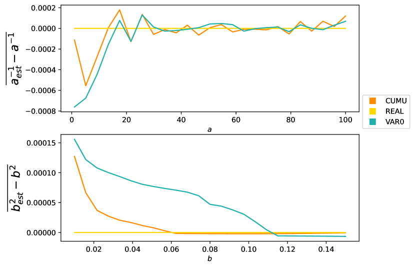
The comparison method used in figure 1 comes from the fact that both equations 10 and 12 are polynomial of $\frac{1}{a}$ and $b^{2}$. Thus, because we used an unbiased estimator for $\kappa_{2}$ and $\kappa_{3}$, Cumulant is nearly unbiased with respect to this formula when $a$ is large enough that $\frac{1}{a^{2}}$ is small in the formula of $\kappa_{3}$. However, we see from figure 1 that it is indeed the case for high values of $a$ and $b$ but not for low values of $a$ and $b$. This can be explained by the fact that we only kept realistic values of $b$. Indeed, if we had kept every estimation of $b^{2}$, we would have had a mean of $0$. Since we only kept values of $b^{2}$ that are higher than $0$, we have a positive bias. Equation 10 shows that under-estimating $b$ leads to an over-estimation of $1/a$ which makes assuming $b^{2}=0$ and re-do calculation of $a$ based on that a way to help minimize bias. Although bias is not that important because for small values of $b$ it results a misestimation of $b^{2}$ and not biasedness of our method. Figure 1 also shows that Variance is always biased for $b$ while Cumulant seems to settle down at $b\approx.06$.

Looking at bias as a function of both $a$ and $b$ and not only $a$ or $b$ gives interesting insights on the way Variance and Cumulant estimates $a$ and $b$.

Figure 2: Bias of $a_{est}$ and $b_{est}$ for Variance.

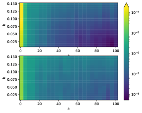
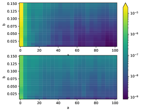
V-D2 Bias as a function of $a$ and $b$

For readability, in this section, we removed the columns corresponding to the two smallest values of $a$.

Figure 3: Bias of $a_{est}$ and $b_{est}$ for Cumulant.

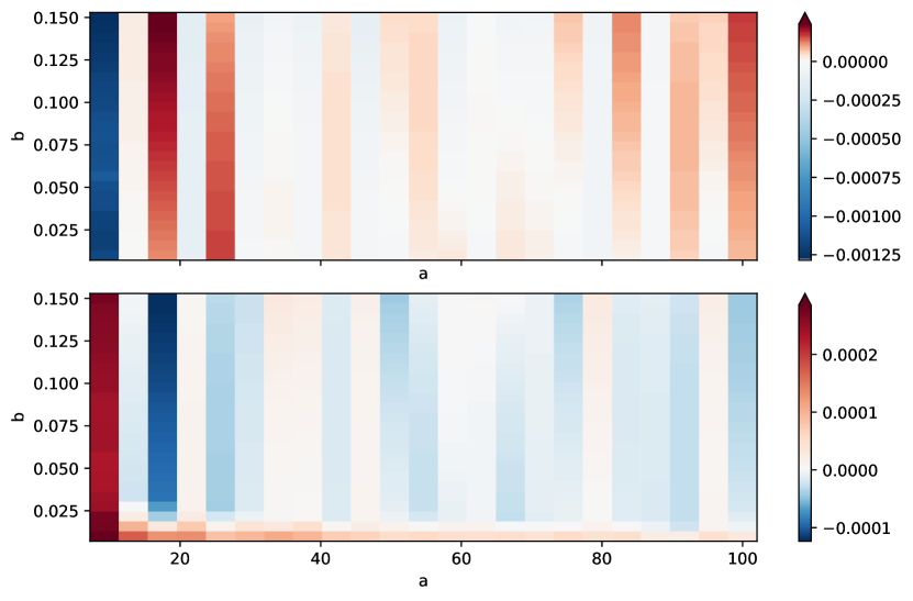
Figure 2 and figure 3 are picturing columns that show the bias on $a_{est}$ or $b_{est}$ as a function of $a_{real}$ and $b_{real}$. In both figures, we see a high dependence from the sign of the bias on $a_{real}$. We do not have an exact explanation on that, but it may be a result of implementation of the noise generator more than a ground truth for the methods. This hypothesis also lean on the fact that Cumulant should be unbiased, and figure 3 happens to have the same bias on the same columns as figure 2. We can also see that whenever a column in biased toward positive for $a$ then it is biased for $b$ but the other way around, which highlights the confusion of the noise parameters. Even if it may look like Variance and Cumulant are biased the same way, dry results IV shows that this is not the case.

TABLE IV: Bias of Variance and Cumulant

	$a$	$b$
4Same bias	29290	28824
Opposite bias	27261	26550

Figure 4: Bias of $a_{est}$ and $b_{est}$ for Cnn.

Figure 5: Bias of $a_{est}$ and $b_{est}$ for Foi et al..

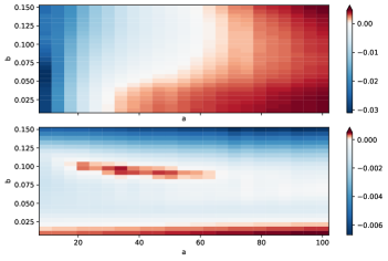
Moreover, figure 4 shows bias toward the extrema of $a$ for the bias of $a$ and $b$ for the bias of $b$. This can be caused by the Cnn being bad on the limits of its training set. However, Cnn does not seem to recognize the notion of noise as there is no dependency of the bias on $a$ with the bias on $b$.

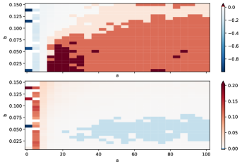
Looking at figure 5 shows that Foi et al. positive bias on $a$ is explained by negative bias on $b$ and vice-versa. This shows that Cnn could learn this behavior as Foi et al. and Cnn take the same input.

In section V-D1 we said the bias is caused by the removal of unrealistic values of $b_{est}$. In the next section, we will analyze up to what extent this is true.

V-D3 Realistic estimations

Figure 6: Percentage of realistic $b_{est}$ for each method.

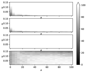
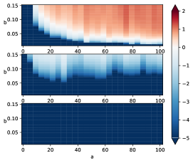
It is found that every method is finding realistic $a$ (except Foi et al.). This does not sound absurd as our range of $a$ (up to $a=100$) allowed misestimation of $\frac{1}{a}$ up to $10^{-2}$ which is greater than what we found with Variance and Cumulant in figure 8.

For Cnn the reason is different, the architecture forced the values of $a_{est}$ and $b_{est}$ to be inside the range of the training set. Interesting result about Foi et al. is that $a_{est}$ was realistic if and only if $b_{est}$ was. This is not the case for the other methods, as shown in figure 6. Cnn finds every $b_{est}$ again by construction. However, we can see noticeable difference between Variance and Cumulant when it comes to the proportion of realistic $b_{est}$ found.

Figure 7: Relative quantity of realistic $b_{est}$, the redder, the more Variance found $b_{est}$ compared to Cumulant

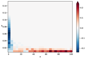
Figure 7 highlights the difficulties of Variance to realistically estimate $b$ when it is small, while Cumulant seems to have more difficulties when it comes to small $a$. For Cumulant, this can be explained by the variance on $\kappa_{3}$ as this variance is dependent on $a^{-1}$ thus greater when $a$ is small. Since $a_{cumulant}$ only depends on $\kappa_{3}$, the precision of $a_{cumulant}$ depends on the precision of the estimation of $\kappa_{3}$ which depends directly on $a_{real}$.

Figure 8: Mean squared error for each method as a function of $a$ (top) and $b$ (bottom).

V-E Mean squared error

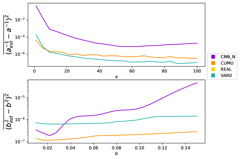
The MSE of $\hat{a}$ is dependent on $a$. We see on Figure 8 that the smaller $a$, the worst the estimation is. This is a consequence of using $\frac{1}{a}$. When $a$ is small, the Poisson noise is more present and when $a$ increases it is disappearing, all of our methods seems to be better at recognizing small noise over a lot of noise even though the MSE on $b$ does not seem to depend a lot on the value of $b$ for both Variance and Cumulant.

We also see that both of the presented methods are better than Cnn at finding result. We also see that Cumulant is 10 times better than Variance at estimating $b$ for this error.

V-F Outliers

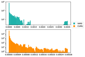
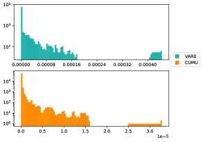
When evaluating our methods, we realized that some outliers have a big influence on the overall performance. So, in this section, we show how they impact the estimations.

Figure 9: Distribution of $MSE(a)$ for Variance and Cumulant

Figure 10: Distribution of $MSE(b)$ for Variance and Cumulant

Figure 11: $MSE(a)$ of Variance and Cumulant after removing outliers

Figure 12: $MSE(b)$ of Variance and Cumulant after removing outliers

V-G Noise-free image dependence

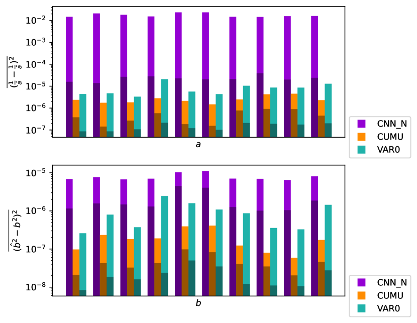
Here, we plot the dependence of the MSE on the $10$ round-truth image $x$ that was used to synthesize the noisy image $y$. We average over the $10$ different seeds and the $b$ or $a$ values respectively. One can observe that the ground-truth data, the image properties, have some influence on the estimation performance, more notably so on the estimation of $b$.

Figure 13: MSE depending on image for $a$ (top) and $b$ (bottom) with or without outliers (darkened)

V-H Log-likelihood

For all the different data samples we have created for comparing the different methods with each other, we additionally computed their log-likelihood values. Those give another interesting perspective on the quality of those estimations.

In terms of trying to maximize the likelihood, Cnn does not work as good as the other methods, as seen from Figure 14.

Figure 14: Difference $\mathcal{LL}$ of Variance and Cumulant

VI Conclusion

In this project, it’s found and proven that Poisson-Gaussian noise modeling is properly matched with raw-data of digital sensors. In this modeling, noise can be decomposed into two parts: Poisson and Gaussian part, where the former one is signal dependent, while the latter is signal independent. We can also relate Poisson effect with discrete nature of photon counting process. Based on this noise modelling, we defined two noise parameters and throughout the project, we tried to propose the algorithmic solution for this. Firstly, the likelihood function is derived as we also have the ground truth image as input. Then, to obtain the good estimation, we tried to obtain maximum likelihood solution of the noise parameter estimation. It’s shown that it’s practically inefficient to be implemented. Therefore, another types of solutions were proposed. Two methods are proposed with using the statistical property of the noise modeling. The methods are Variance and Cumulant, where they use variance and cumulant information, respectively. Cumulant was found to be better at estimating values when $a$ was small, while Variance was found to be better when $b$ was small. For the real cases, Poisson part can dominate the noise, which means $a$ is small. Thus, we can conclude that Cumulant is more robust for real-world cases. Also, Variance relies on discrete intensities, which may not be realistic.

Also, to compare the proposed methods with the solution found in the literature, two more algorithms were tested: Foi et al. and Cnn. It’s found that both Variance and Cumulant are better than these methods for MSE and likelihood comparison. Also, it’s found that all these methods might be used as a starting point for maximization of likelihood for the future works.

Another future work might be listed as adjusting the weights for the Variance method, considering the clipping behavior of the images in real-world. Throughout the experiment, we didn’t clip any images, which are not the case in the real world. For the last thing to do might be adding the efficient maximization of likelihood.

-A Derivation of Maximum Likelihood Solution

-A1 Poisson-Noise Modeling

Let us denote observed noisy image as $y$ and ground-truth image as $x$. Then, Poisson-Gaussian modelling can be explained from 14.

$$y=\frac{1}{a}\alpha+\beta,\quad\alpha\sim\mathcal{P}(ax),\quad\beta\sim\mathcal{N}(0,b^{2})$$ (14)

When expectation of both sides are taken, the following equation 15 is obtained with the use of linearity property of expectation.

$$\mathbb{E}[y]=\frac{1}{a}\mathbb{E}[\alpha]=\frac{1}{a}ax=x$$ (15)

When variance is applied to both sides in 14, the following equation 16 is obtained.

$$\mathbb{V}[y]=\mathbb{E}\left[\left(\frac{1}{a}\alpha+\beta\right)^{2}\right]-x^{2}=\frac{1}{a^{2}}\mathbb{E}[\alpha^{2}]+b^{2}-x^{2}$$ (16)

Given $\mathbb{E}[\alpha^{2}]=ax+a^{2}x^{2}$, we have:

$$\mathbb{V}[y]=\frac{x}{a}+x^{2}+b^{2}-x^{2}=\frac{x}{a}+b^{2}$$ (17)

-A2 Likelihood Function of Single-Pixel Image

From the definition of the probability mass function of a Poisson random variable, the following equation 18 is obtained.

$$\mathbb{P}(\{\alpha=k\})=\frac{e^{-ax}(ax)^{k}}{k!},\quad k\geq 0$$ (18)

From the relation between probability density function (PDF) and probability mass function (PMF) of discrete random variable with the use of Dirac delta function, i.e. $f_{X}(t)=\sum_{k\in\mathbb{Z}}\mathbb{P}(\{X=k\})\delta(t-k)$, we have:

$$f_{\alpha}(t|a,x)=\sum_{k=0}^{\infty}\frac{e^{-ax}(ax)^{k}}{k!}\delta(t-k)$$ (19)

Let us define $\alpha^{\prime}=\frac{1}{a}\alpha$. Then, the cumulative distribution function (CDF) of this random variable $\alpha^{\prime}$ can be found as following:

$$F_{\alpha^{\prime}}(t)=\mathbb{P}(\{\alpha^{\prime}\leq t\})=\mathbb{P}(\{\alpha\leq at\})=F_{\alpha}(at)$$ (20)

When taking the derivative of equation 20 is taken, the PDF can be found as:

$$f_{\alpha^{\prime}}(t)=\frac{dF_{\alpha^{\prime}}(t)}{dt}=\frac{dF_{\alpha}(at)}{dt}=af_{\alpha}(at)$$ (21)

As $\alpha$ and $x$ are given, the likelihood function of Poisson part can be found as following:

$$\begin{split}f_{\alpha^{\prime}}(t|a,x)&=a\sum_{k=0}^{\infty}\frac{e^{-ax}(ax)^{k}}{k!}\underbrace{\delta(at-k)}_{=\frac{1}{a}\delta(t-\frac{k}{a})}\\ &=\sum_{k=0}^{\infty}\frac{e^{-ax}(ax)^{k}}{k!}\delta(t-k/a)\end{split}$$ (22)

The likelihood function of a Gaussian random variable with $0$ mean is as following:

$$f_{\beta}(t|b)=\frac{1}{b\sqrt{2\pi}}e^{-t^{2}/2b^{2}}$$ (23)

Let us find the likelihood function of $y$. Since we know that $\alpha^{\prime}$ and $\beta$ are independent to each other, we have:

$$\begin{split}f_{y}(y|a,b,x)&=(f_{\alpha^{\prime}}*f_{\beta})(y|a,b,x)\\ &=\sum_{k=0}^{\infty}\frac{(ax)^{k}}{k!b\sqrt{2\pi}}\exp{\left(-ax-\frac{(y-k/a)^{2}}{2b^{2}}\right)}\end{split}$$ (24)

-A3 Maximum Likelihood Solution for Single-Pixel Image

Thus, the maximum likelihood solution for a single-pixel image is as following:

$$\begin{split}\hat{a},\hat{b}&=\arg\max_{a,b}f_{y}(y|a,b,x)\\ &=\arg\max_{a,b}\sum_{k=0}^{\infty}\frac{(ax)^{k}}{k!b\sqrt{2\pi}}\exp{\left(-ax-\frac{(y-k/a)^{2}}{2b^{2}}\right)}\end{split}$$ (25)

-A4 Likelihood Function of Multi-Pixel Image

We can denote images as vectors of pixels, like $y_{n}$ and $x_{n}$ where $n\in\mathbb{N}$. Hence, we have the following:

$$f_{y}(y_{n}|a,b,x)=\sum_{k=0}^{\infty}\frac{(ax_{n})^{k}}{k!b\sqrt{2\pi}}\exp{\left(-ax_{n}-\frac{(y_{n}-k/a)^{2}}{2b^{2}}\right)}$$ (26)

Given $x$, i.e., the vector that contains all $x_{n}$, it can be seen that $y_{n}$ and $y_{n^{\prime}}$ are independent, $\forall n\neq n^{\prime}$. Therefore, we have:

$$f_{y}(y|a,b,x)=\prod_{n}\sum_{k=0}^{\infty}\frac{(ax_{n})^{k}}{k!b\sqrt{2\pi}}\exp{\left(-ax_{n}-\frac{(y_{n}-k/a)^{2}}{2b^{2}}\right)}$$ (27)

-A5 Maximum Likelihood Solution for Multi-Pixel Image

Hence, we get the following maximization problem:

$$\begin{split}\hat{a},\hat{b}=\arg\max_{a,b}\prod_{n}\sum_{k=0}^{\infty}\frac{(ax_{n})^{k}}{k!b\sqrt{2\pi}}\exp{\left(-ax_{n}-\frac{(y_{n}-k/a)^{2}}{2b^{2}}\right)}\end{split}$$ (28)

Using the strict monotonicity of the logarithm, we can simplify the optimization problem while not altering its results.

$$\begin{split}\hat{a},\hat{b}=&\arg\max_{a,b}\\ &\sum_{n}\log{\left(\sum_{k=0}^{\infty}\frac{(ax_{n})^{k}}{k!b\sqrt{2\pi}}\exp{\left(-ax_{n}-\frac{(y_{n}-k/a)^{2}}{2b^{2}}\right)}\right)}\end{split}$$ (29)

In order to be computable, we limit the range of $k$ to a maximum value $k_{max}$ which has to be chosen big enough to get a good approximation.

$$\begin{split}\hat{a},\hat{b}\approx&\arg\max_{a,b}\\ &\sum_{n}\log{\left(\sum_{k=0}^{k_{max}}\frac{(ax_{n})^{k}}{k!b\sqrt{2\pi}}\exp{\left(-ax_{n}-\frac{(y_{n}-k/a)^{2}}{2b^{2}}\right)}\right)}\end{split}$$ (30)

-B Cumulant

-B1 Some properties

-B2 $\kappa_{r}$

For a random variable $X$ following the distribution $\mathcal{X}$, we consider the cumulant-generating function defined as :

$$K_{\mathcal{X}}(t)=\log(\mathbb{E}[e^{Xt}])$$

Then we define $\kappa_{r}$the $r^{th}$ cumulant of $\mathcal{X}$ as:

$$\kappa_{r}:=K_{\mathcal{X}}^{(r)}(0)$$

with $K_{\mathcal{X}}^{(r)}(0)$ being the $r$-th derivative of $K_{\mathcal{X}}$ evaluated in $0$.

-B3 Linearity

The cumulant-generating function of a sum of independent distribution is the sum of their cumulant-generating function :

$$\begin{split}K_{\mathcal{X}+\mathcal{Y}}(t)&=\log(\mathbb{E}(e^{(X+Y)t}))\\ &=\log(\mathbb{E}[e^{Xt+Yt}])\\ &=\log(\mathbb{E}[e^{Xt}e^{Yt}])\\ &=\log(\mathbb{E}[e^{Xt}]\mathbb{E}[e^{Yt}])\\ &=\log(\mathbb{E}[e^{Xt}])+\log(\mathbb{E}[e^{Yt}])\\ &=K_{\mathcal{X}}(t)+K_{\mathcal{Y}}(t)\end{split}$$ (31)

-B4 Homogeneous of degree

The $r^{th}$ cumulant is homogeneous of degree $r$ :

$$\kappa_{r}(a\mathcal{X})=a^{r}\kappa_{r}(\mathcal{X})$$ (32)

-B5 Unbiased estimator

For a vector $x$ obtained by sampling independently and identically $n$ times from the law $\mathcal{X}$, [24] describes an unbiased estimator of $\kappa_{2,3}$, the $r^{th}$ cumulant of $\mathcal{X}$ with :

$$\begin{split}\kappa_{2}(\mathcal{X})=\frac{n}{n-1}m_{2}(x),\quad\kappa_{3}(\mathcal{X})=\frac{n^{2}}{(n-1)(n-2)}m_{3}(x)\end{split}$$

With $m_{2}$ the sample variance and $m_{3}$ the $3^{rd}$ sample central moment, that can be calculated using the formulas taken from [25] :

$$\begin{split}m_{2}(x)&=\frac{n-1}{n}\sum_{i}(x_{i}-\overline{x})^{2}\\ m_{3}(x)&=\frac{(n-1)(n-2)}{n^{2}}\sum_{i}(x_{i}-\overline{x})^{3}\end{split}$$

-B6 Cumulant of Poisson-Gaussian Noise

We have $\mathcal{Y}\sim\frac{\mathcal{P}(a\mathcal{X})}{a}+\mathcal{N}(0,b^{2})$, we want to have a $\kappa_{2}(\mathcal{Y})$ and $\kappa_{3}(\mathcal{Y})$ as a function of $a$ and $b$. First, we use equation 31 : $\kappa_{r}(\mathcal{Y})=\kappa_{r}(\frac{\mathcal{P}(a\mathcal{X})}{a})+\kappa_{r}(\mathcal{N}(0,b^{2}))$.

-B7 Gaussian noise component

The cumulant of $\mathcal{N}(0,b^{2})$ are known :

$$\begin{split}\kappa_{2}(\mathcal{N}(0,b^{2}))&=b^{2}\\ \kappa_{3}(\mathcal{N}(0,b^{2}))&=0\end{split}$$ (33)

-B8 Poisson noise component

Instead of trying to find the cumulant of $\frac{\mathcal{P}(a\mathcal{X})}{a}$, we can use equation 32 and find the cumulant of $\mathcal{Z}\sim\mathcal{P}(a\mathcal{X})$.

$$e^{K_{\mathcal{Z}}(t)}=\sum_{k}\mathbb{P}[Z=k]e^{tk}$$

Moreover, we know that :

$$\begin{split}\mathbb{P}[Z=k]&=\sum_{i}\mathbb{P}[X=x_{i}]\mathbb{P}[Z=k|X=i]\\ &=\sum_{i}n_{i}\frac{(ax_{i})^{k}e^{-ax_{i}}}{k!}\end{split}$$

where $n_{i}=\frac{\left|\set{j:x_{j}=x_{i}}\right|}{n}$, the proportion of intensities equal to the one of $x_{i}$.

Thus :

$$\begin{split}e^{K_{\mathcal{Z}}(t)}&=\sum_{k}\mathbb{P}[Z=k]e^{tk}\\ &=\sum_{k}\sum_{i}n_{i}\frac{(ax_{i})^{k}e^{-ax_{i}}}{k!}\exp(t)^{k}\\ &=\sum_{i}n_{i}\frac{e^{-ax_{i}}}{exp(-ax_{i}e^{t})}\sum_{k}\frac{(ax_{i}e^{t})^{k}\exp(-ax_{i}e^{t})}{k!}\\ &=\sum_{i}n_{i}\exp(ax_{i}(e^{t}-1))\end{split}$$

If we note : $f:t\rightarrow\sum_{i}n_{i}\exp(ax_{i}(e^{t}-1))$ Then : $K_{\mathcal{Z}}(t)=\log(f(t))$ We have :

$$\begin{split}K_{\mathcal{Z}}(t)&=\log(f(t))\\ K_{\mathcal{Z}}^{1}(t)&=\frac{f^{(1)}(t)}{f(t)}\\ K_{\mathcal{Z}}^{2}(t)&=\frac{f^{(2)}(t)f(t)-f^{(1)}(t)^{2}}{f(t)^{2}}\\ K_{\mathcal{Z}}^{3}(t)&=\frac{f(t)[f(t)f^{(3)}(t)-3f^{(2)}(t)f^{(1)}(t)]+2f^{(1)}(t)^{3}}{f(t)^{3}}\\ K_{\mathcal{Z}}^{4}(t)&=\frac{f^{(4)}(t)}{f(t)}-\frac{f^{(1)}(t)f^{(3)}(t)}{f(t)^{2}}\\ &-3\frac{f^{(3)}(t)f^{(1)}(t)+f^{(2)}(t)^{2}}{f(t)^{4}}\\ &+12\frac{f^{(1)}(t)^{2}f^{(2)}(t)}{f(t)^{3}}-6\frac{f^{(1)}(t)^{4}}{f(t)^{4}}\\ \end{split}$$

With

$$\begin{split}f(0)&=1\\ f^{(1)}(0)&=a\overline{x}\\ f^{(2)}(0)&=a\overline{x}+a^{2}\overline{x^{2}}\\ f^{(3)}(0)&=a\overline{x}+3a^{2}\overline{x^{2}}+2a^{3}\overline{x^{3}}\\ f^{(4)}(0)&=a^{4}\overline{x^{4}}+7a^{3}\overline{x^{3}}+7a^{2}\overline{x^{2}}+a\overline{x}\\ \end{split}$$

Thus :

$$\begin{split}K_{\mathcal{Z}}(0)&=0\\ K_{\mathcal{Z}}^{1}(0)&=a\overline{x}\\ K_{\mathcal{Z}}^{2}(0)&=a\overline{x}+a^{2}\overline{x^{2}}-a^{2}\overline{x}^{2}\\ K_{\mathcal{Z}}^{3}(0)&=a^{3}[\overline{x^{3}}-3\overline{x^{2}}\overline{x}+2\overline{x}^{3}]+a^{2}[3\overline{x^{2}}-3\overline{x}^{2}]+a\overline{x}\end{split}$$

Now, using equation 32, we have :

$$\begin{split}\kappa_{2}\left(\frac{\mathcal{P}(a\mathcal{X})}{a}\right)&=\frac{\overline{x}}{a}+\overline{x^{2}}-\overline{x}^{2}\\ \kappa_{3}\left(\frac{\mathcal{P}(a\mathcal{X})}{a}\right)&=\overline{x^{3}}-3\overline{x^{2}}\overline{x}+2\overline{x}^{3}+3\frac{\overline{x^{2}}}{a}-3\frac{\overline{x}^{2}}{a}+\frac{\overline{x}}{a^{2}}\end{split}$$ (34)

-B9 Everything together

By putting equations 33 and 34 together, we have :

$$\begin{split}\kappa_{2}(\mathcal{Y})&=\frac{\overline{x}}{a}+\overline{x^{2}}-\overline{x}^{2}+b^{2}\\ \kappa_{3}(\mathcal{Y})&=\overline{x^{3}}-3\overline{x^{2}}\overline{x}+2\overline{x}^{3}+3\frac{\overline{x^{2}}}{a}-3\frac{\overline{x}^{2}}{a}+\frac{\overline{x}}{a^{2}}\end{split}$$

References

- [1] A. Foi, M. Trimeche, V. Katkovnik, and K. Egiazarian, “Practical Poissonian-Gaussian noise modeling and fitting for single-image raw-data,” IEEE Transactions on Image Processing, vol. 17, no. 10, pp. 1737–1754, 2008.
- [2] F. Luisier, T. Blu, and M. Unser, “Image denoising in mixed Poisson-Gaussian noise,” IEEE Transactions on Image Processing, vol. 20, no. 3, pp. 696–708, 2011.
- [3] M. Aharon, M. Elad, and A. Bruckstein, “K-SVD: An algorithm for designing overcomplete dictionaries for sparse representation,” IEEE Transactions on Signal Processing, vol. 54, no. 11, pp. 4311–4322, 2006.
- [4] S. Gu, L. Zhang, W. Zuo, and X. Feng, “Weighted nuclear norm minimization with application to image denoising,” in Computer Vision and Pattern Recognition (CVPR), 2014.
- [5] K. Dabov, A. Foi, V. Katkovnik, and K. Egiazarian, “Image denoising by sparse 3-D transform-domain collaborative filtering,” IEEE Transactions on Image Processing, vol. 16, no. 8, pp. 2080–2095, 2007.
- [6] D. Zoran and Y. Weiss, “From learning models of natural image patches to whole image restoration,” in International Conference on Computer Vision (ICCV), 2011.
- [7] T. Huang, S. Li, X. Jia, H. Lu, and J. Liu, “Neighbor2Neighbor: A self-supervised framework for deep image denoising,” IEEE Transactions on Image Processing, 2022.
- [8] X. Ma, X. Lin, M. El Helou, and S. Süsstrunk, “Deep Gaussian denoiser epistemic uncertainty and decoupled dual-attention fusion,” in IEEE International Conference on Image Processing (ICIP), 2021, pp. 1–4.
- [9] K. Zhang, W. Zuo, and L. Zhang, “FFDNet: Toward a fast and flexible solution for CNN-based image denoising,” IEEE Transactions on Image Processing, vol. 27, no. 9, pp. 4608–4622, 2018.
- [10] M. El Helou and S. Süsstrunk, “Blind universal Bayesian image denoising with Gaussian noise level learning,” IEEE Transactions on Image Processing, vol. 29, pp. 4885–4897, 2020.
- [11] M. El Helou and S. Süsstrunk, “BIGPrior: Towards decoupling learned prior hallucination and data fidelity in image restoration,” IEEE Transactions on Image Processing, 2022.
- [12] M. El Helou, R. Zhou, and S. Süsstrunk, “Stochastic frequency masking to improve super-resolution and denoising networks,” in European Conference on Computer Vision (ECCV), 2020, pp. 749–766.
- [13] Q. Wang, X. Zhang, Y. Wu, L. Tang, and Z. Zha, “Nonconvex weighted minimization based group sparse representation framework for image denoising,” IEEE Signal Processing Letters, vol. 24, no. 11, pp. 1686–1690, 2017.
- [14] S. Cai, Z. Kang, M. Yang, X. Xiong, C. Peng, and M. Xiao, “Image denoising via improved dictionary learning with global structure and local similarity preservations,” Symmetry, vol. 10, no. 5, p. 167, May 2018. [Online]. Available: http://dx.doi.org/10.3390/sym10050167
- [15] S. Cai, K. Liu, M. Yang, J. Tang, X. Xiong, and M. Xiao, “A new development of non-local image denoising using fixed-point iteration for non-convex sparse optimization,” PLOS ONE, vol. 13, no. 12, pp. 1–24, 12 2018. [Online]. Available: https://doi.org/10.1371/journal.pone.0208503
- [16] Y. Zhang, Y. Zhu, E. Nichols, Q. Wang, S. Zhang, C. Smith, and S. Howard, “A Poisson-Gaussian denoising dataset with real fluorescence microscopy images,” in Proceedings of the IEEE/CVF Conference on Computer Vision and Pattern Recognition, 2019, pp. 11 710–11 718.
- [17] R. Zhou, M. El Helou, D. Sage, T. Laroche, A. Seitz, and S. Süsstrunk, “W2S: microscopy data with joint denoising and super-resolution for widefield to SIM mapping,” in European Conference on Computer Vision Workshops, 2020, pp. 474–491.
- [18] A. Jezierska, H. Talbot, C. Chaux, J.-C. Pesquet, and G. Engler, “Poisson-gaussian noise parameter estimation in fluorescence microscopy imaging,” in 2012 9th IEEE International Symposium on Biomedical Imaging (ISBI), 2012, pp. 1663–1666.
- [19] B. Zhang, “Contributions to fluorescence microscopy in biological imaging: PSF modeling, image restoration, and super-resolution detection,” Ph.D. dissertation, Télécom ParisTech, Informatics, telecommunications and electronics (EDITE), Paris, France, Nov. 2007. [Online]. Available: https://pastel.archives-ouvertes.fr/pastel-00003273
- [20] N. Bähler, M. El Helou, É. Objois, K. Okumuş, and S. Süsstrunk, “Pogain: Poisson-gaussian image noise modeling from paired samples,” IEEE Signal Processing Letters, pp. 1–5, 2022.
- [21] H. J. Trussell and R. Zhang, “The dominance of poisson noise in color digital cameras,” in 2012 19th IEEE International Conference on Image Processing, 2012, pp. 329–332.
- [22] D. P. Kingma and J. Ba, “Adam: A method for stochastic optimization,” 2017.
- [23] D. Martin, C. Fowlkes, D. Tal, and J. Malik, “A database of human segmented natural images and its application to evaluating segmentation algorithms and measuring ecological statistics,” in Proc. 8th Int’l Conf. Computer Vision, vol. 2, July 2001, pp. 416–423.
- [24] E. W. Weisstein, “k-statistic from mathworld–a wolfram web resource.” [Online]. Available: https://mathworld.wolfram.com/k-Statistic.html
- [25] ——, “Sample central moment. from mathworld–a wolfram web resource.” [Online]. Available: https://mathworld.wolfram.com/SampleCentralMoment.html